Northumbria Research Linknrl.northumbria.ac.uk/33708/1/Ocean-forced ice... · Northumbria Research...

Northumbria Research Link

Citation: Jordan, Jim, Holland, Paul, Goldberg, Dan, Snow, Kate, Arthern, Robert, Campin, Jean-Michel, Heimbach, Patrick and Jenkins, Adrian (2018) Ocean-Forced Ice-Shelf Thinning in a Synchronously Coupled Ice-Ocean Model. Journal of Geophysical Research: Oceans, 123 (2). pp. 864-882. ISSN 2169-9275

Published by: Wiley-Blackwell

URL: https://doi.org/10.1002/2017JC013251 <https://doi.org/10.1002/2017JC013251>

This version was downloaded from Northumbria Research Link: http://nrl.northumbria.ac.uk/33708/

Northumbria University has developed Northumbria Research Link (NRL) to enable users to access the University’s research output. Copyright © and moral rights for items on NRL are retained by the individual author(s) and/or other copyright owners. Single copies of full items can be reproduced, displayed or performed, and given to third parties in any format or medium for personal research or study, educational, or not-for-profit purposes without prior permission or charge, provided the authors, title and full bibliographic details are given, as well as a hyperlink and/or URL to the original metadata page. The content must not be changed in any way. Full items must not be sold commercially in any format or medium without formal permission of the copyright holder. The full policy is available online: http://nrl.northumbria.ac.uk/pol i cies.html

This document may differ from the final, published version of the research and has been made available online in accordance with publisher policies. To read and/or cite from the published version of the research, please visit the publisher’s website (a subscription may be required.)

http://nrl.northumbria.ac.uk/policies.html

Confidential manuscript submitted to JGR-Oceans

Ocean-forced ice-shelf thinning in a synchronously coupled1

ice–ocean model2

James R. Jordan1, Paul R. Holland1, Dan Goldberg2, Kate Snow2, Robert Arthern1,3

Jean-Michel Campin3, Patrick Heimbach4and Adrian Jenkins14

1British Antarctic Survey, High Cross, Madingley Road, Cambridge, CB3 0ET, UK52University of Edinburgh, School of GeoSciences, Edinburgh, UK6

3Department of Earth, Atmospheric and Planetary Sciences, Massachusetts Institute of Technology, 77 Massachusetts7

Avenue, Cambridge, MA, USA84The University of Texas at Austin, Institute for Computational Engineering and Sciences (ICES), 201 East 24th Street,9

Austin, TX, USA10

Key Points:11

• The first synchronously coupled, fully conservative ice shelf–ocean model has been12

developed.13

• Unlike a parameterised melt simulation, coupled runs have asymmetric ice-shelf14

topography.15

• For a given ice-shelf mass, parameterising melt tends to underestimate ice-shelf16

buttressing.17

Corresponding author: James R. Jordan, [email protected]

–1–


Abstract18

The first fully synchronous, coupled ice shelf–ocean model has been developed using the19

MITgcm (Massachusetts Institute of Technology general circulation model). Unlike pre-20

vious, asynchronous, approaches to coupled modelling our model is fully conservative21

of heat, salt and mass. Coupling at the ocean time step level is achieved by converting22

melt rates (represented as mass fluxes) to corresponding ice shelf volume, i.e. geometry23

changes, and minimizing spurious barotropic and baroclinic adjustment processes. By sim-24

ulating an idealised, warm-water ice shelf we show how raising the pycnocline leads to25

a reduction in both ice-shelf mass and back stress, and hence buttressing. Coupled runs26

show the formation of a western boundary channel in the ice-shelf base due to increased27

melting on the western boundary due to Coriolis enhanced flow. Eastern boundary thick-28

ening is also observed. This is not the case when using a depth-dependent parameterised29

melt, as the ice shelf has relatively thinner sides and a thicker central ‘bulge’ for a given30

ice-shelf mass due to the lack of coupled feedbacks arising from rotation driven flow. Ice-31

shelf geometry arising from a parameterised melt rate tends to underestimate backstress32

for a given ice-shelf mass due to a thinner ice shelf at the boundaries when compared to33

coupled model simulations. By arbitrarily assigning a minimum melting depth in a depth-34

dependent melt-rate parametrisation a minimum ice-shelf thickness is imposed, which can35

lead to inaccurate estimations of ice-shelf buttressing.36

1 Introduction37

Melting beneath floating ice shelves, which accounts for roughly half of the fresh-38

water flux from Antarctica [Depoorter et al., 2013], takes place where sufficiently warm39

ocean water makes contact with the ice-shelf base. Cooling of continental shelf waters by40

sea ice growth protects much of the Antarctic margin from the warm Circumpolar Deep41

Water (CDW) of the Southern Ocean [Jacobs et al., 1992]. However, in some locations of42

both the West Antarctic Ice Sheet (WAIS) [Walker et al., 2007; Petty et al., 2013; Dutrieux43

et al., 2014] and East Antarctic Ice Sheet (EAIS) [Greenbaum et al., 2015; Silvano et al.,44

2016], deep ocean troughs and weaker ice growth allow warm CDW to infiltrate the con-45

tinental shelf. Where this occurs, melt rates can reach tens of metres per year or higher46

[Jacobs et al., 1996].47

The mechanism by which this melting affects sea-level rise is indirect, since thinning48

of ice shelves has negligible direct contribution. Rather, thinning of an ice shelf affects49

the restraining force (often termed ‘buttressing’) that the ice shelf provides to the ice sheet50

that feeds it [Dupont and Alley, 2005]. With a lessening of this restraint, ice would flow51

into the ocean at a greater rate and there might be retreat of the grounded ice sheet extent,52

or grounding line, leading to sea-level rise [Thomas et al., 1979].53

Buttressing is provided by slow-moving ice at the side margins of embayed ice shelves,54

or by ‘pinning points’ (areas of grounded ice within the ice shelf) [Thomas, 1979]. Strong55

increases in seaward grounded ice fluxes have been observed as a result of ice-shelf thin-56

ning [Shepherd et al., 2004] and disintegration [Scambos et al., 2004]. Improved under-57

standing of the response of ice sheets to ice-shelf thinning is therefore vital to constraining58

future behaviour of the Antarctic Ice Sheet under differing climate scenarios. Attempts to59

quantify this response are complicated, however, by the possibility of feedbacks within the60

ice–ocean system.61

Our understanding of the dynamics of coupled ice–ocean behaviour is hampered62

by the lack of existing models that can suitably represent ice–ocean interactions [Joughin63

et al., 2012]. Ocean models have difficulties accounting for continuously changing ice-64

margin geometry, and ice models are only now approaching a level at which interactions65

between floating and grounded ice can be correctly represented [Pattyn and Durand, 2013;66

Favier et al., 2014].67

–2–


In this work we present the first truly synchronous, coupled ice shelf–ocean model68

and use it to investigate the effects of ocean temperature variation on ice-shelf buttressing.69

The coupled model is described, along with the process of online adaptation of the ice–70

ocean boundary. We also compare our coupled results to an ice model forced by a simple71

depth-dependent parameterised melt rate, and compare the effects upon buttressing of the72

two methods.73

2 Approaches to coupled modelling74

Ice shelf–ocean coupling can be approached in a number of ways that fall into three75

broad categories, which we refer to as ‘discontinuous’, ‘asynchronous’ and ‘synchronous’76

coupling. While describing these approaches we refer to the time step of both the ocean77

and ice components of the coupled model as well as a separate, coupled time step. This78

coupled time step is defined to be the interval between the exchange of melt rate and ice-79

shelf thickness between the ice and ocean models.80

‘Discontinuous’ coupling initialises a new ocean model every one or few ice timesteps,81

with each new ocean model having a different ice-shelf geometry. The coupled time step82

is therefore of the order of the ice time step. The ocean model is spun-up from suitable83

initial conditions and fixed boundary conditions, and then the steady-state ocean melt rate84

is used in the continuously running ice model for the entire next coupled time step. From85

a practical standpoint this approach tends to be very easy to implement, as the coupling86

process is all done offline using the existing model initialisation code. This approach is87

computationally cheap, with the expensive ocean model run time kept to a minimum as88

it is not running continuously (although some spin-up time between coupled time steps is89

required). However, as the ocean history is discarded for each new initialisation, the cou-90

pled model does not conserve heat, salt and mass between coupled time steps. This ap-91

proach cannot be used with rapidly varying forcings because the ocean model history must92

be maintained in these circumstances. It also cannot be used in global coupled climate93

models (GCMs), which cannot repeatedly spin-up their ocean model. Examples of models94

that use this approach are Goldberg et al. [2012a], Goldberg et al. [2012b], Gladish et al.95

[2012] and De Rydt and Gudmundsson [2016].96

In ‘asynchronous’ coupling both the ice and ocean models are run simultaneously,97

exchanging information between them every one or few ice timesteps. The coupled time98

step is therefore similar to that of a discontinuous approach. This approach is slightly99

more complex than discontinuous coupling, as some modification of the ocean state is100

required every coupling timestep to account for changing ice topography instead of restart-101

ing the ocean model each time from arbitrary initial conditions. The computational ex-102

pense is basically the same as running uncoupled ocean and ice models. This is more ex-103

pensive than discontinuous coupling, due to the need to continuously run the ocean model104

for the entire ice simulation. Moving from one fixed ice shelf topography to another at105

the coupling step leads to continuity issues with mass, heat, salt and momentum in the106

ocean that has to be solved with ad-hoc techniques. This could lead to problems when us-107

ing GCMs to consider sea level rise (mass) and warming (heat), as well as barotropic and108

baroclinic adjustments leading to ‘tsunamis’ throughout the model domain (velocity). The109

melt rate used in the ice model can lack detail both spatially and temporally as it is ap-110

plied over an entire coupled time step rather than evolving along with ocean conditions, as111

well as being spatially averaged from the ocean grid to the ice grid. Examples of this ap-112

proach are Seroussi et al. [2017], Asay-Davies (2017, personal communication) and Robin113

Smith (2017, personal communication).114

The final approach, described in this manuscript, is that of ‘synchronous’ coupling.115

In this approach the ocean and ice models are both continuously run, with the coupled116

time step being the same as the ocean time step rather than of the order of the ice time117

step as in the previous two approaches. From a practical point of view this is more diffi-118

–3–


cult to achieve, as the ocean model code needs to be change ice shelf geometry every time119

step, as well as properly interface with the ice-shelf code within a simulation. This ap-120

proach can also be more expensive than asynchronous coupling as the ice model is being121

solved every ocean time step, and needs to share the ocean grid. However, this approach122

is fully conservative of heat, salt and mass, which makes it well-suited to problems with123

rapidly varying forcing and for use in GCMs. The model described in this manuscript is124

the first ice–ocean model to use this approach.125

3 Coupled model126

Throughout this work we use the MITgcm (Massachusetts Institute of Technology127

general circulation model) to model the complete ice–ocean system by coupling an ocean128

model (that can represent ice shelves) to an ice stream/shelf model. Both models being129

contained within the MITgcm framework vastly simplifies the coupling process, enabling130

a fully conservative, fully coupled ice–ocean model within one executable code. Note we131

only test this model in an ice shelf–ocean context; the implementation of grounded ice132

is discussed in a paper in preparation. A list of all parameters, their symbols and given133

values used throughout this manuscript can be found in Table 1.134

Before going into detail about the individual parts of the model our approach to135

synchronous coupling can be summarised as follows. Melt rates from the ocean model136

viewed as vertical mass fluxes of freshwater are used to change the ice shelf thickness in137

the ice model at every ocean time step. The thinning ice shelf leads to a reduced pres-138

sure load on the ocean from the ice shelf, which in turn leads to an inflow of ocean from139

surrounding cells. This results in the sea surface rising, resulting in a reduced ice shelf140

draft. The changing shape of the ice shelf draft will affect ocean dynamics and the result-141

ing melt rate, bringing us full circle.142

3.1 Ocean model143

3.1.1 Existing model144

The ocean is simulated using the MITgcm [Marshall et al., 1997], a z-level coordi-145

nate model. The model utilises the partial-cell functionality for topography [Adcroft et al.,146

1997] combined with a non-linear ocean free surface that can change the partial-cell thick-147

ness in time [Campin et al., 2004]. This allows more accuracy than a fixed ∆z when rep-148

resenting both ocean floor bathymetry and ice-shelf basal topography. When using partial149

cells it is useful to define the open-cell fraction150

hc =R∆z, (1)

where R is the vertical size of the cell and ∆z is the vertical grid spacing (defined at each151

model z-level and may vary with depth). The fraction hc is therefore usually 1, except152

potentially in the topmost and bottommost cells. The fraction hc changes temporally in153

line with the ocean free surface and can become both greater than or less than 1 [Campin154

et al., 2004].155

The ice shelf forcing on the ocean is implemented using a method akin to that of156

Losch [2008]. The vertical position of the ice–ocean interface, zsur f , is defined relative157

to a reference ice-shelf basal depth, d, which itself is defined to adhere strictly to vertical158

grid boundaries (see section 3.1.3). When hc in the topmost cell is equal to 1 this means159

zsur f is located at the top most cell boundary. The position of the ice–ocean interface rel-160

ative to the reference depth is defined as η. These relations are shown in Fig. 1(a) and161

allow us to express the vertical position of the ice–ocean interface as162

–4–


zsur f = d + η. (2)

3.1.2 Thermodynamics166

The ice-shelf melt-rate is calculated using the three-equation formulation (Jenkins167

et al. [2010]) with constant non-dimensional heat and salt transfer coefficients (ΓT and ΓS ,168

respectively) and friction velocity (u∗). The three equation melt rate formation is given by169

mL = ρiciκi∂Ti∂z

��b

− ρswcswu∗ΓT (Tb − T) (3)170

Tb = aSb + b + cz (4)171

m(Sb − Si) = −ρswu∗ΓS(Sb − S) (5)

with m the ablation rate of ice (expressed as a mass change per unit time, positive for172

melting), ρi and ρsw the density of ice and seawater, respectively, L the latent heat of ice173

fusion, ci and csw the specific heat capacity of ice and seawater respectively, u∗ the fric-174

tion velocity, κi the thermal diffusivity of ice, ∂Ti∂z��bthe temperature gradient at the ice–175

ocean boundary, Tb (assumed to be at the pressure dependent freezing temperature) and176

Sb the temperature and salinity at the ice–ocean interface, T and S the ‘far-field’ ocean177

temperature and salinity in the boundary layer, a, b, and c are constants, and Si is the178

salinity of ice.179

This leads to a flux of heat (FT ) and salt (FS) across the boundary [Jenkins et al.,180

2001], defined as;181

FT = −ρswcsw(ΓT (Tb − T) − Ûmρi(Tb − Tsur f )) (6)182

FS = −ρsw(ΓS(Sb − S) − Ûmρi(Sb − Ssur f )) (7)

with Tsur f and Ssur f the temperature and salinity of the model cell containing the ice–183

ocean interface. These salt and heat fluxes are applied using the boundary-layer method184

of Losch [2008] in combination with an input of a ‘real’ meltwater mass flux (FW ) in a185

manner akin to that used to simulate evaporation and precipitation, making the model fully186

conservative of heat, salt and mass. The mass flux input in this case is equivalent to the187

water released with an ablation rate of m, ie;188

FW = m (8)

The ocean properties T , S, and u∗ used in this formulation are a weighted average189

of a boundary layer (Bχ for tracer properties and Bv for velocities) over a distance of ∆z190

from the ice–ocean interface (Fig. 1b). The formulation requires u∗ to be defined at the191

same location as the tracer properties temperature and salinity. As MITgcm uses a c-grid,192

the weighted average over ∆z of the four horizontally adjacent points on the velocity grid193

to the tracer point in question is used. This gives rise to a friction velocity u∗ that is used194

in melt rate calculations, defined as;195

u∗2 = Cd(V2top +U2

top) (9)

where Cd is the dimensionless ice-shelf drag coefficient and Vtop and Utop are the average196

v and u velocities in the boundary layer, each composed of up to 4 grid velocities.197

In contrast to the current version of MITgcm, we define the boundary layer velocity198

to be over ∆z of water from the ice–ocean interface at the velocity points rather than at199

the tracer points (Fig. 1b). This ensures that no zero velocities at grid walls are averaged200

–5–


into u∗. In practice this results in the ocean velocity being relatively larger in our method201

compared to the previous implementation, and minimising the impact of grid discretisa-202

tion. A z-level model, such as the MITgcm, tends to give ’stripy’ melt rates of alternating203

high and low melt rates when d differs between two neighbouring cells in the horizontal204

plane. This leads to the cells being at different z levels and having a reduced u∗ due to205

the no-flow conditions at the velocity points on vertical ice-shelf faces. In the implemen-206

tation of Losch [2008], the model grid was defined so that the topmost wet cells, if partial207

cells, had thickness less than ∆z. In our implementation having cells larger than ∆z is un-208

avoidable, which initially led to a worsening of the ‘stripy’ melt rate artifact seen in Losch209

[2008]. Our method of calculating u∗ acts to minimise this by ensuring that no ‘zero flow’210

are averaged into u∗. Furthermore, the model remeshing described later (section 3.1.4) has211

the added benefit of evolving the discretisation during the simulation, limiting the impact212

of this problem at any given location.213

3.1.3 Pressure214

The momentum solver in MITgcm does not use pressure p directly, but rather pressure-215

potential which is simply defined as φ = pρre f

in the Boussinesq framework. Additionally216

the baroclinic pressure gradient is found directly from the perturbation to the geopotential,217

φ′ = φ − φre f = φ −

∫ 0

z

gdz. (10)

with g being the acceleration due to gravity. The perturbed geopotential at z can be writ-218

ten as219

φ′ =φ′d + g(zsur f − d) +∫ zsur f

z

gρ − ρre f

ρre fdz

=φ′d + gη +

∫ zsur f

z

gρ − ρre f

ρre fdz (11)

where the first term is due to the load placed at the reference surface d (or rather, the load220

minus the background potential); the second is due to the variation of the free surface221

zsur f from the reference surface, and the third is the vertical integral of buoyancy leading222

to the baroclinic pressure. Note that the integral in the third term has upper bound zsur f223

rather than d and no approximation of buoyancy is used over the interval [d, zsur f ]. This224

is due to our use of the non-linear free surface capability of the ocean model [Campin225

et al., 2004]. In this implementation, the free surface η adjusts each time step as part of226

the barotropic mass and momentum stepping. The work of Losch [2008] generalised this227

formulation to allow d to be located at the base of the ice shelf rather than at sea level. In228

our coupling implementation, φ′dis the geopotential perturbation associated with the ice229

overburden:230

φ′d = g

(ρiHρre f

− d)

(12)

where ρiH is the ice shelf mass per unit area, with H being the ice thickness. This allows231

changes in ice thickness to be translated to changes in surface pressure at each ocean time232

step, therefore permitting a coupled time step that is the same as the ocean time step.233

Note this approach is distinct from the approach of Losch [2008] which does not ex-234

plicitly specify ice mass, but rather specifies d as the ‘target’ ice draft and defines φ′dsuch235

that η = 0 (and thus the ocean surface is at d) when the ocean is quiescent with the initial236

density profile. Our approach also differs from Losch [2008] in that d now is at the same237

depth as vertical grid boundaries, yielding values of η that are potentially large even when238

–6–


the ocean is stagnant. This is not an issue, however, as it can be seen from (11) and (12)239

that the geopotential is invariant to a redefinition of d, as long as η is similarly redefined240

to keep zsur f unchanged.241

In order to avoid cell thicknesses that are too large (increasing discretisation error),242

or are negative, d will eventually need to be modified (described later in section 3.1.4).243

Changing d every timestep in response to changing ice-shelf mass, however, is costly as it244

would require a redefinition of the linear system that is solved for the free surface update245

[Campin et al., 2004]. A compromise, then, is to only change d when remeshing occurs,246

which necessarily means that η will undergo variations of order ∆z. We choose to align d247

with vertical cell faces for ease of development.248

3.1.4 Remeshing249

We have developed the MITgcm such that the evolving ice sheet model and ice250

shelf melting changes the ocean domain, with the ocean mesh evolving accordingly. The251

use of partial cells leads to top cells with varying hc in both time and space, with prob-252

lems arising for too large or small an hc . Too large an hc leads to a poor representation253

of the boundary layer required for calculating the melt rate, whilst too small an hc can254

lead to unrealistically high velocities. If either occurs it is necessary to update the model255

grid. Upon initialisation of MITgcm, ocean model grid cells are flagged as being either256

ice or ocean. The remeshing process described here essentially allows ocean model cells257

to switch from ice to ocean, and vice versa, within a model run and without the need to258

reinitialise initial ice and ocean masks. Whilst hc continuously evolves every time step, at259

a predetermined interval (dtremesh) we check to see if it has grown above hmax or below260

hmin. If it has then we trigger the remesh process, essentially redefining d, the reference261

depth of the ice shelf that the position of the ocean free surface (zsur f , located at the ice–262

ocean interface under an ice shelf) is relative to.263

This is done by either splitting a cell with too large an hc into two smaller cells or264

merging a cell with too small an hc with another cell to create a single large cell. This265

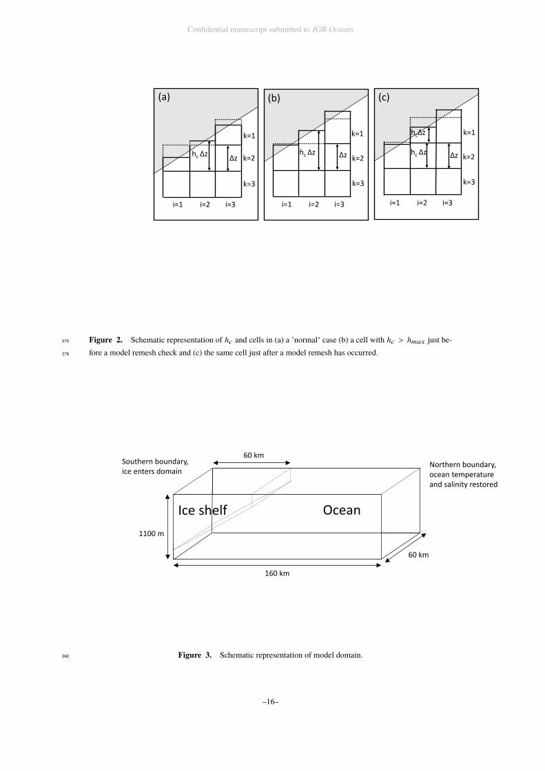
process is shown in Fig. 2. Fig. 2(a) shows the top layer of partial cells under an ice266

shelf. As the ice-shelf melts its thickness decreases, raising the position of the ice–ocean267

interface and thus increasing the cells volume by FW . This leads to cell i = 2, k = 2268

to have a larger hc than hmax (Fig. 2(b)). The cell is then split into two new cells, posi-269

tioned at i = 2, k = 2 and i = 2, k = 1 respectively (Fig. 2(c)). Similarly, when merging270

a cell with hc less than hmin with the cell below, the process happens in reverse. If cell271

i = 2, k = 1 in Fig. 2(c) were too small it would need to be merged with i = 2, k = 2. The272

resultant cell, i = 2, k = 2 in Fig. 2(b), would have the combined hc of cells i = 2, k = 1273

and i = 2, k = 2 from Fig. 2(c).274

When a cell is split into new cells all tracer properties are conserved, with the two277

new cells taking the properties of the old cell.278

χold = χlower = χupper (13)where χold is a tracer property of the old cell being split into upper and lower cells with279

tracer properties χlower and χupper respectively. The same relationship holds for veloci-280

ties on all faces, however when new cell creation leads to a new solid ice boundary (as in281

Fig. 2) then the velocity on this boundary is set to zero. The hc of the two new cells are282

given by;283

holdc ∆zold = hlower

c ∆zlower + hupperc ∆zupper = ∆zlower + (holdc − 1)∆zupper (14)

where holdc , hlower

c (equal to 1 in this case) and hupperc the dimensionless size of the old,284

large cell and two new cells, respectively, whilst ∆zold , ∆zlower and ∆zupper are the ver-285

–7–


tical grid spacing of the same. Note that ∆zold is the same as ∆zlower . As there has been286

a change in the cells masked as ice or ocean we also need to update the reference position287

of the ice shelf, d.288

dnew = dold + ∆zold (15)

where dold is the old reference depth of the ice shelf and dnew is the new reference po-289

sition. During this process, the vertical position of the ocean free surface never changes,290

such that in the top most ocean cell;291

znewsur f = dnew + ηnew = dold + ηold = zoldsur f (16)

where zoldsur f

, zoldsur f

and ηold, ηnew are the old and new positions of the ice–ocean interface292

and its distance from the reference depth of the ice shelf respectively.293

When merging two cells with hlowerc (=1), χlower and hupperc , χupper respectively294

then (14) and (15) still apply, only in reverse, but (13) becomes;295

χlower hlowerc + χupper hupperc

hnewc

= χnew (17)

which also holds for velocities on cell faces.296

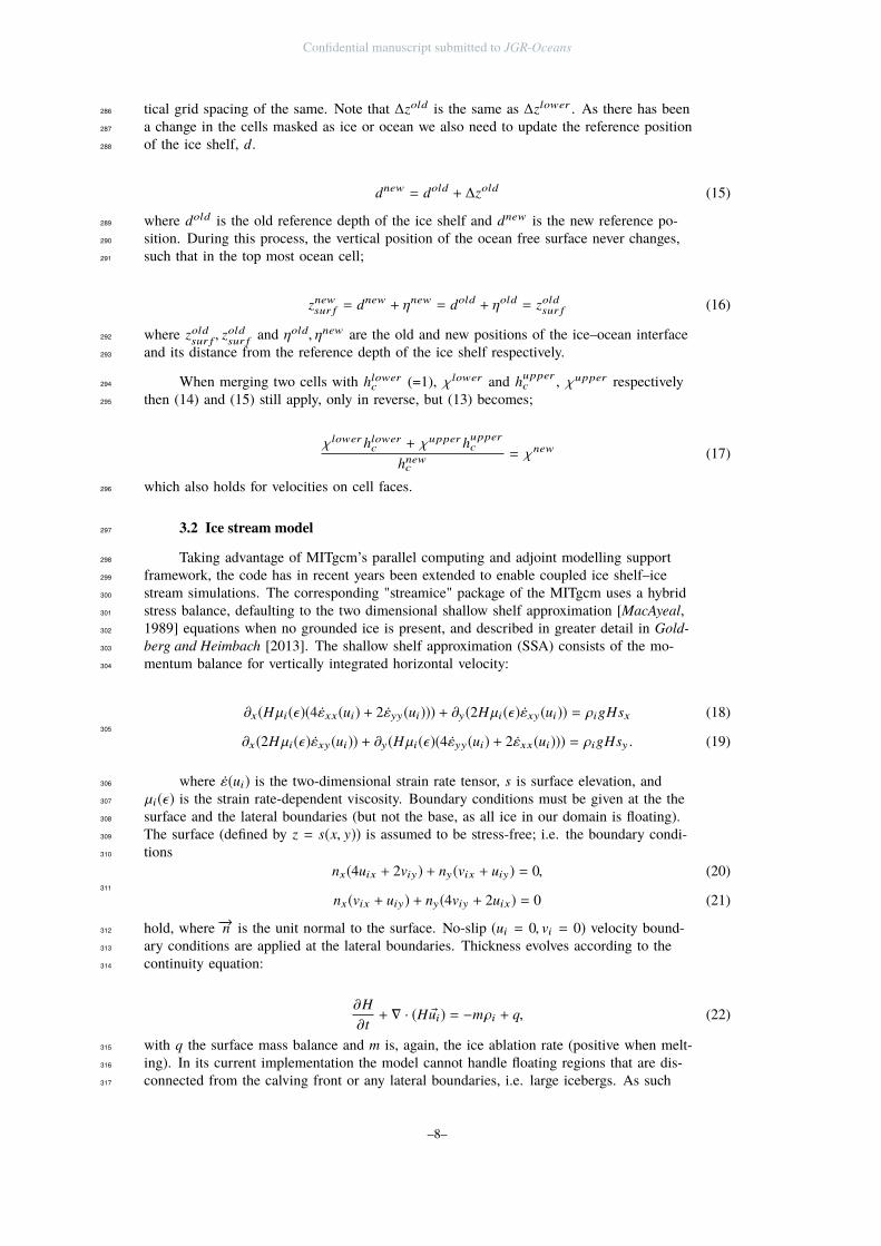
3.2 Ice stream model297

Taking advantage of MITgcm’s parallel computing and adjoint modelling support298

framework, the code has in recent years been extended to enable coupled ice shelf–ice299

stream simulations. The corresponding "streamice" package of the MITgcm uses a hybrid300

stress balance, defaulting to the two dimensional shallow shelf approximation [MacAyeal,301

1989] equations when no grounded ice is present, and described in greater detail in Gold-302

berg and Heimbach [2013]. The shallow shelf approximation (SSA) consists of the mo-303

mentum balance for vertically integrated horizontal velocity:304

∂x(Hµi(ε)(4 Ûεxx(ui) + 2 Ûεyy(ui))) + ∂y(2Hµi(ε) Ûεxy(ui)) = ρigHsx (18)305

∂x(2Hµi(ε) Ûεxy(ui)) + ∂y(Hµi(ε)(4 Ûεyy(ui) + 2 Ûεxx(ui))) = ρigHsy . (19)

where Ûε(ui) is the two-dimensional strain rate tensor, s is surface elevation, and306

µi(ε) is the strain rate-dependent viscosity. Boundary conditions must be given at the the307

surface and the lateral boundaries (but not the base, as all ice in our domain is floating).308

The surface (defined by z = s(x, y)) is assumed to be stress-free; i.e. the boundary condi-309

tions310

nx(4uix + 2viy) + ny(vix + uiy) = 0, (20)311

nx(vix + uiy) + ny(4viy + 2uix) = 0 (21)

hold, where −→n is the unit normal to the surface. No-slip (ui = 0, vi = 0) velocity bound-312

ary conditions are applied at the lateral boundaries. Thickness evolves according to the313

continuity equation:314

∂H∂t+ ∇ · (H ®ui) = −mρi + q, (22)

with q the surface mass balance and m is, again, the ice ablation rate (positive when melt-315

ing). In its current implementation the model cannot handle floating regions that are dis-316

connected from the calving front or any lateral boundaries, i.e. large icebergs. As such317

–8–


we impose a minimum value of ice thickness (Hmin), typically of a few centimetres. It is318

assumed that ice that has reached this thickness has completely melted away.319

In this study the ice domain consists of the ice shelf only, with an imposed inflow320

velocity. In the experiments below, we examine the stress state and diagnose the total but-321

tressing, i.e. the integrated shear stress along the ice shelf sidewalls. In doing so, we ne-322

glect potentially important feedbacks such as changes in inflow velocity, and lengthening323

of the ice shelf further due to grounding line retreat (along with potential further changes324

to inflow speed due to variable topography). These feedbacks have been observed to oper-325

ate on longer time scales than those of coupled ice shelf–ocean evolution, however [Gold-326

berg et al., 2012b; Seroussi et al., 2017]. Grounding line migration maintains the potential327

to be an issue with a suitably steep bed geometry over these timescales, however this is328

not a concern with the flat geometry used here. In this sense our study looks at the early329

response in buttressing to coupled ice shelf–ocean evolution. The synchronous coupled330

model is currently being further developed to allow a fully moving grounding line.331

The interface between ice and ocean involves passing the ice thickness H to the332

ocean code which calculates φ′d, and using the melt rate calculated by the ocean model333

to update the ice shelf mass balance (22). Using an inbuilt ice sheet code makes it easy334

to do this on a per-ocean timestep basis. Solving (18) and (19) in each ocean time step335

would be prohibitively expensive; this is because the system of PDEs is non-local and336

non-linear (with the viscosity dependant upon the velocity field), and is solved through an337

iterative procedure, with each iteration requiring the solution of a large linear system. On338

the other hand, the change in velocity associated with thickness change over an ocean time339

step is negligible. In our time stepping strategy, (22) is implemented each ocean time step340

with the latest ocean melt rate. A single iteration of the solver for (18) and (19) is com-341

puted every ice time step to update ice velocities and it is assumed that thickness change342

over this period is sufficiently small that only a single iteration is required. A similar ‘split343

time step’ strategy was used by Walker and Holland [2007]. With this time stepping strat-344

egy, the ice model comprises ∼1-2% of the total coupled model run time. Therefore the345

cost of the coupled model is essentially the same as that of the ocean model alone.346

4 Experimental design347

Our test domain is designed to represent a typical warm-water ice shelf, such as348

Pine Island Glacier (PIG). The domain is 60 km wide and 160 km long, with a depth of349

1100 m (Fig. 3). The ice shelf has an initial extent of 60 km, beyond which it is not al-350

lowed to advance, although retreat is possible through thinning to the minimum ice-shelf351

thickness. The ice shelf flows into the domain through a boundary we refer to as ‘south’,352

and calves in the opposite direction which we refer to as ‘north’. A coupled time step of353

60 s has been used throughout. The coupled model was run for a period of 60 years with354

monthly output, and all simulations had reached a steady-state by the end of this period.355

As well as these coupled runs, ice only runs with parameterised melt rates were carried356

out for the same forcings. In all cases we are interested in how the ice-shelf thickness357

evolves over time and its impact upon ice-shelf backstress (and therefore buttressing).358

Constants not explicitly defined have the values given in Table 1.359

The ocean model mesh is 160 by 60 cells in the horizontal with a 1 km grid res-361

olution and 55 cells in the vertical with a constant ∆z of 20 m grid resolution. No slip362

boundary conditions are applied to ocean velocities at the east, west and south as well as363

the ocean floor and ice–ocean interface, whilst no slip boundary conditions are applied364

to the ice at the east and west. Temperature and salinity are restored to initial conditions365

at the northern boundary in a 5 cell wide linear sponge layer over a time period of one366

day. To account for the changing ocean volume within the domain due to the flux of ice367

across the calving front, the average open-ocean sea-surface height (SSH) is restored to368

zero through adjustment of the open boundary barotropic velocity. That is, if there is a369

–9–


net mass loss of ice in the closed domain, to prevent continually sinking SSH upon ad-370

justment, there will be a small net inflow of water across the northern boundary, restored371

to the prescribed temperature and salinity, which ensures the open-ocean SSH is always372

maintained to a zero average. Horizontal diffusivity and viscosity are both set to a con-373

stant 100 m2 s−1, whilst vertical diffusivity and viscosity are 1 × 10−3 m2 s−1 and 5 × 10−5374

m2 s−1 respectively. An ocean time step of 60 s has been used throughout, except for the375

first month of the ‘Warm’ simulation (see below), where a time step of 30 s was required376

to prevent a failure of the model to converge. Rotation is accounted for by means of an f377

plane at the equivalent of 70 ◦S.378

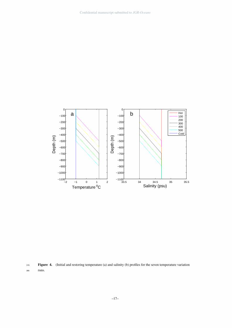
Initial temperature and salinity profiles for the baseline case have warm, salty wa-381

ter (1.2 ◦C, 34.7 psu) at depth and cold, fresh water at the surface (-1 ◦C, 34 psu). These382

two water masses are separated by a linearly varying pycnocline of 400 m thickness, start-383

ing at 300 m depth. These temperature and salinity profiles are consistent with previous384

work on PIG [De Rydt et al., 2014]. Sensitivity studies have been carried out around this385

baseline by varying the depth of the pycnocline by ± 100 m and 200 m in both directions,386

but maintaining its thickness of 400 m. This gives us five different forcings, henceforth re-387

ferred to by the depth of the upper limit of the pycnocline (100, 200, 300 (baseline), 400,388

500). A ‘Warm’ and ‘Cold’ run were also carried out, with water conditions constant in389

depth (and hence no pycnocline) at the previously mentioned warm and cold water masses390

(Fig. 4).391

The ice model mesh extends 60 km from the southern boundary, sharing a grid with392

the 1 km horizontal resolution ocean mesh. The initial ice-shelf geometry was generated393

by running the ice stream model on its own without any basal melting until steady-state.394

A Glen’s law exponent of n = 3 is used in combination with a Glen’s law coefficient of395

B=4.9 × 105 Pa yr−13 (corresponding to an ice temperature of roughly -15 ◦ C). Ice en-396

ters the domain with a constant flux, achieved by maintaining a fixed ice-shelf draft of 900397

m at the southern boundary along with an inflow velocity that peaks at 2 km a−1 in the398

center of the domain and falls to 0 km a−1 at the margins. Ice that moves past the calving399

front located 60 km from the southern boundary is removed from the domain. Ice veloci-400

ties within the domain are updated at the ice time step of 43200 s, whilst ice thickness is401

updated every coupled time step which is the same as the ocean time step of 60 s.402

5 Results403

5.1 Time stepping comparison404

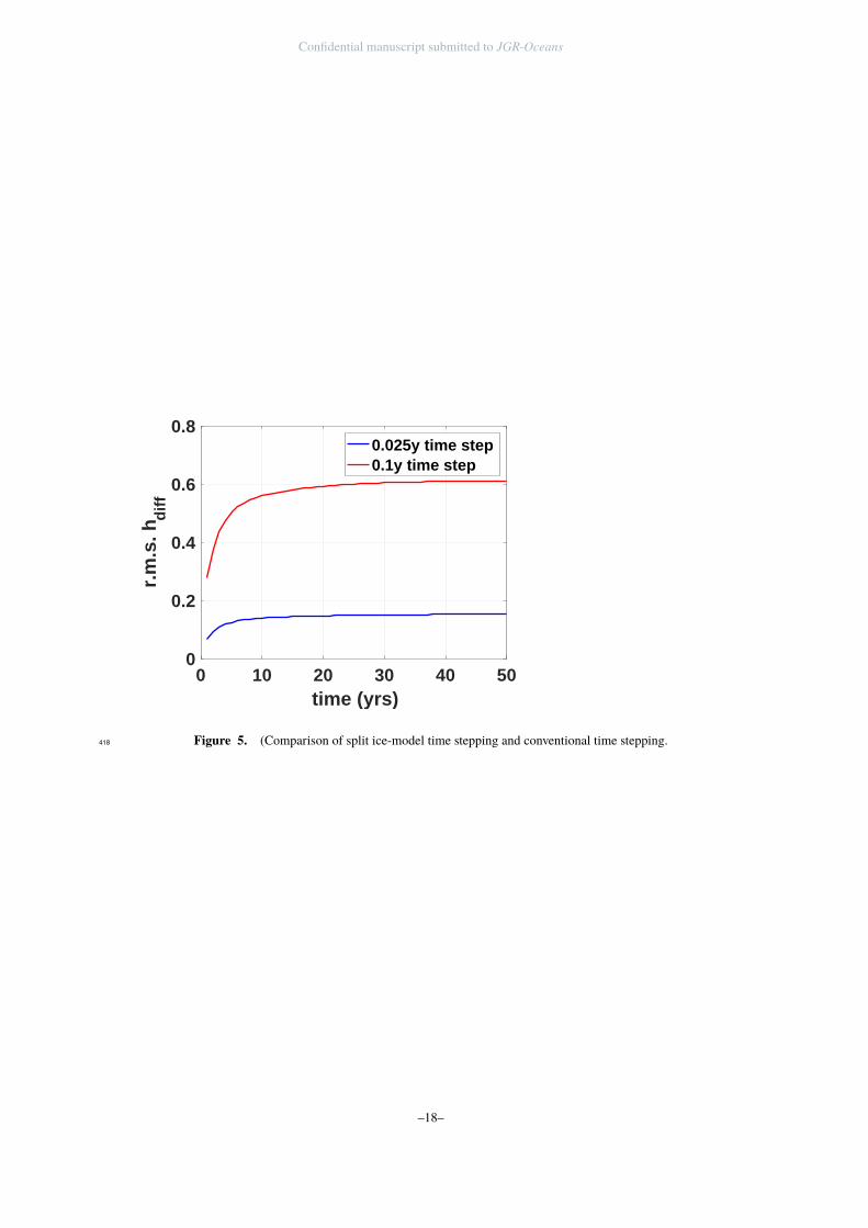
Before presenting results we briefly compare the accuracy of our ice model split405

time stepping with more traditional ice sheet time stepping. We carry out an ice-only ex-406

periment with ice domain and model parameters as described above, where an initially407

steady ice shelf is forced by a constant melt rate of 5 m a−1 and allowed to evolve. We408

carry out one simulation with split time stepping, where thickness is updated every 360409

s and velocity every 43200 s without convergence. In addition we carry out two simu-410

lations in which the momentum balance is iterated to convergence, and the thickness is411

updated via continuity, on the same time step. Fig. 5 shows the root mean square differ-412

ence in thickness between the simulations. Over 50 years, the difference between split and413

0.1-year time stepping grows to ∼0.6 m, which is small relative to the overall change in414

thickness. Furthermore the comparison with 0.025-year time stepping is only ∼0.15 m,415

implying a linear convergence of the long-timestep simulations toward the split time step416

solution.417

5.2 Baseline simulation time evolution419

In a fully coupled ice-shelf model the ice-shelf geometry affects the ocean flow,420

which in turn affects the melt rate, and thus the ice-shelf geometry. Whilst we will discuss421

–10–


these effects separately it should be noted that they are all happening simultaneously, cre-422

ating feedbacks with one another within the model. We first look at a representative (300423

m pycnocline, baseline) run and examine in detail the processes occurring in the fully cou-424

pled evolution of ice-shelf geometry.425

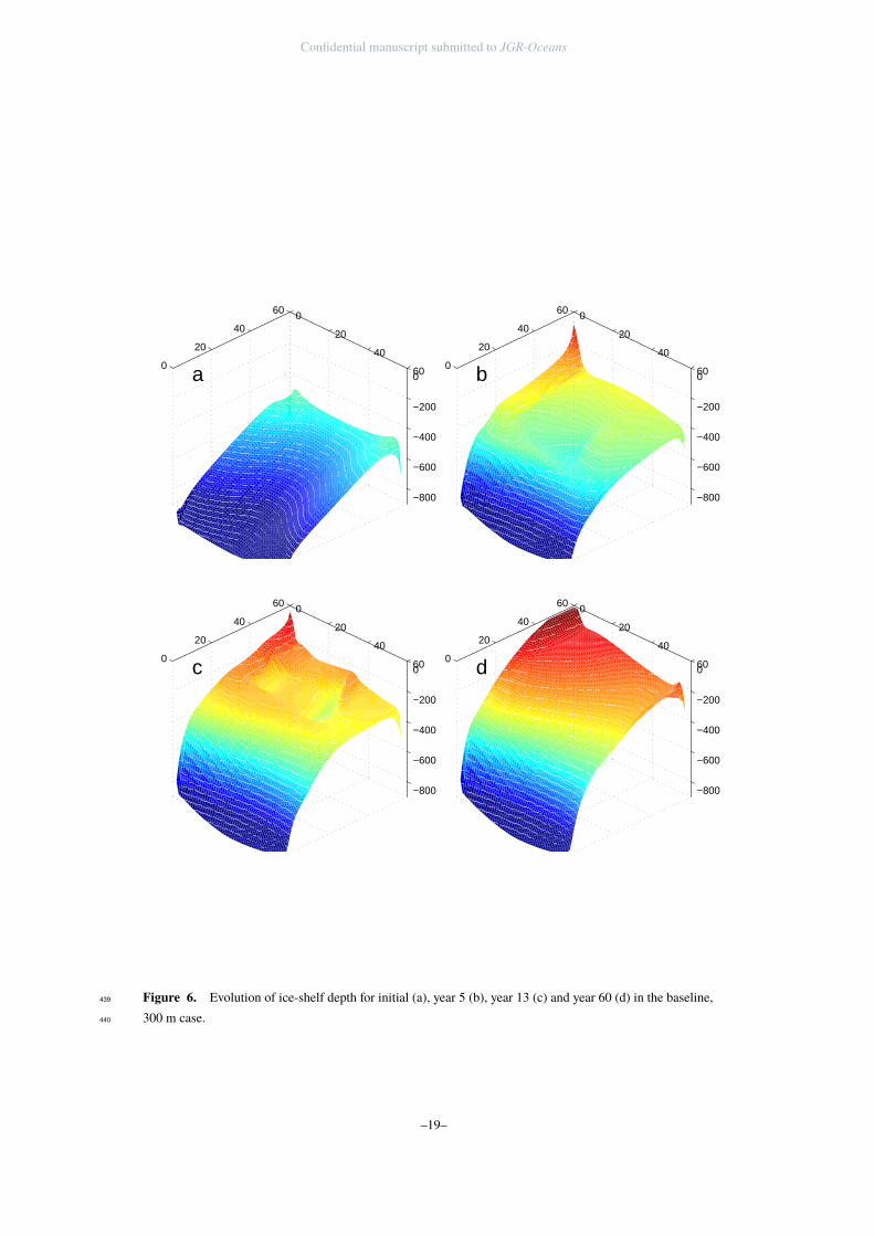
This evolution of the ice-shelf thickness in the baseline run is shown in Fig. 6. Ini-426

tially, the ice is symmetrical in thickness about a central ‘bulge’ (Fig. 6a). When melt-427

ing is applied, however, this symmetry is quickly lost. Within 5 years the ice shelf has428

thinned noticeably, with a pronounced western channel (Fig. 6b). After 13 years the chan-429

nel is still present, although its rate of formation is slowed (Fig. 6c). There are also the430

remnants of the initial central ‘bulge’, which is advected towards the ice front by ice that431

has entered the domain since melting began. This transitory period has ended by the time432

60 years has passed, and a new stable state has established itself (Fig. 6d). This state is433

characterised by the presence of a western channel, although relative to the rest of the434

ice shelf not as deep when compared to the transitory phase. The central ‘bulge’ that was435

present in the initial conditions has now been deflected to the east by preferential melting436

in the west, leading to the western half of the ice shelf being comparatively thinner than437

the eastern half.438

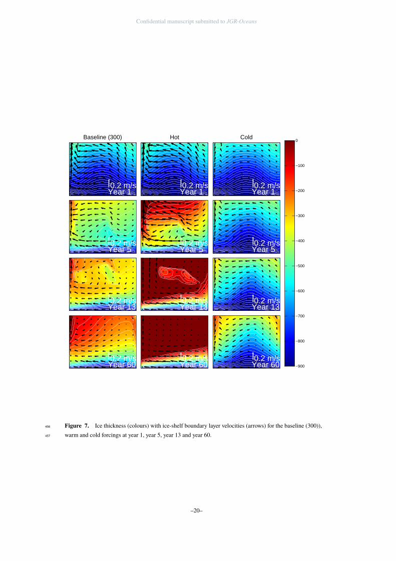
This changing ice-shelf geometry influences the oceanic flow within the model do-441

main (Fig. 7). With the initial geometry, the flow is directed towards the western, Coriolis442

favoured side. The flow moves past the central ‘bulge’ if possible and then flows almost443

due west until it hits the western boundary, creating a strong boundary current. Whilst the444

majority of the flow leaves the ice shelf cavity via the western channel, some flow leaves445

the domain on the eastern side of the ‘bulge’. After 5 years this boundary current has in-446

duced high melting, leading to a self reinforcing channel at the western boundary. The447

central ‘bulge’ is quickly melted away. After 13 years since the beginning of the simula-448

tion there is an overall reduction in boundary layer velocity over much of the shelf, except449

near the grounding line and the western channel. The remnants of the initial ‘bulge’ still450

direct flow around it, although it is quickly being advected off the shelf to be replaced by451

thinner ice that melted nearer the grounding line. The final, steady-state ocean flow main-452

tains the pattern of greatest flow velocity at depth and in the western channel. The central453

‘bulge’ has shifted so far over the eastern side of the shelf that flow is restricted on the454

eastern side.455

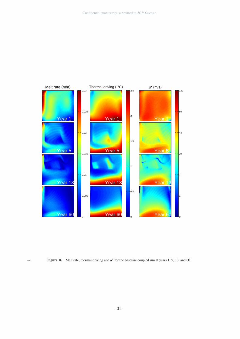
This ocean flow drives the melting of the ice shelf (Fig. 8), which itself is depen-458

dent upon u∗ and thermal driving (T − Tf , where Tf is the pressure dependent freez-459

ing point). Initial conditions show highest melting on the western boundary, as well as460

western side of the ‘bulge’. There are also relatively high melt rates over much of the ice461

shelf. These melt rates are primarily driven by the high initial thermal driving all across462

the ice shelf due to initialising the ice geometry from a non-melting case, with a corre-463

spondingly thicker ice shelf protruding into warmer waters. The only part of the ice shelf464

with low thermal driving is the western channel. As the initial geometry is symmetrical,465

the low thermal driving is a result of the water in the western channel being comprised466

of predominantly melt water which is fresher and colder than the surrounding water. The467

fact the melt water plume in the western channel is less dense than the surrounding wa-468

ter contributes to the high u∗ observed here, greater than anywhere else in the domain.469

After 5 years melt rates have fallen dramatically. High melt rates remain at the ground-470

ing line, where new ice is entering the domain at depth, where thermal driving is great-471

est. Melt rates are low over much of the ice shelf, except in the western channel. The low472

melt rates on the shelf as a whole are a result of low thermal driving and u∗, though the473

central ‘bulge’ is generating high thermal driving when present. The relatively high melt474

rates in the western channel are due to the relatively high u∗ present, as there is still very475

low thermal driving here due to the melt water plume. After 13 years the vast majority476

of ice-shelf melting is happening near the grounding line, with very little melt elsewhere,477

including the western channel. This is despite there being the highest values of u∗ in the478

–11–


western channel. The final, steady-state after 60 years is similar, with melting predom-479

inantly happening at the grounding line due to the combination of high thermal driving480

and u∗. The western channel now acts to channel the release of melt water from the ice481

shelf, with melt rates limited by the low thermal driving of melt water despite a high u∗482

from the western boundary flow.483

5.3 Coupled temperature variation runs485

As well as the baseline (300) case, Fig. 7 also shows the time evolution of the ice-486

shelf depth and boundary layer flow for the warm and cold case.487

The warm case starts from the same initial conditions as the baseline (300) case,488

however due to the increased thermal driving throughout the water column it melts at489

an increased rate. By 5 years there is not only a pronounced western channel, but the490

ice shelf has melted to its minimum thickness in places. Ocean flow is still favouring491

the western side due to Coriolis forcing, with the remains of the initial ‘bulge’ directing492

flow around it. After 13 years the vast majority of the ice shelf has melted to its minimum493

thickness, with the last remnants of the initial ‘bulge’ detaching from the remains of the494

ice shelf as a pseudo-iceberg and subsequently exiting the domain. The steady-state for the495

‘warm’ case has an ice shelf resembling a triangular wedge, slightly thinner on the Corio-496

lis favoured western side.497

In contrast, the cold case does not change greatly from its initial conditions. Whilst498

the imposition of melting causes a slight overall reduction in ice-shelf depth the general499

shape of the ice shelf, including the central ‘bulge’, remains largely intact. There is a500

small change in ice-shelf thickness at the western boundary, but much smaller than in the501

baseline case. Ocean flow is still affected by the presence of the ‘bulge’, needing to find502

its way around it as it heads to the western, Coriolis dominated side.503

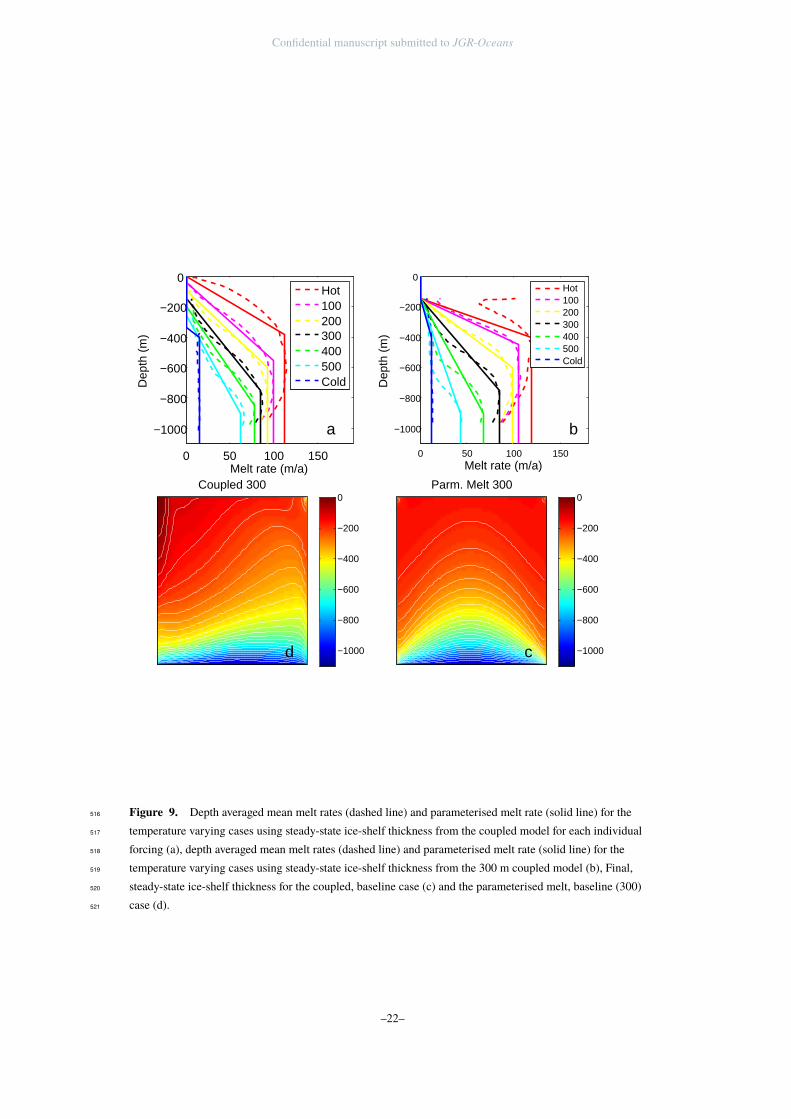
Fig. 9a shows the area averaged (binned every 10 m) steady-state melt rate for the504

various forcing simulations. Depths less than the minimum thickness of the ice shelf have505

zero melt rate whilst maximum melt rates are achieved at a depth just above that of the506

thickest ice. This is due to the greatest u∗ velocities being located just away from the507

southern boundary. Melting does not occur below 900 m depth, due to the incoming ice508

being limited to 900 m depth. Interestingly, despite all cases (except the cold case) having509

the same maximum forcing they do not have the same maximum melt rate. As melt rate is510

a function of both thermal driving and u∗, this would suggest that progressive thinning of511

the ice shelf by means of a higher pycnocline leads to higher ocean velocities, most likely512

due to a combination of a steepening of the ice-shelf gradient and a stronger melt water513

plume. Raising the pycnocline by 100 m sees a reduction in ice-shelf thickness of roughly514

50 m at the calving front.515

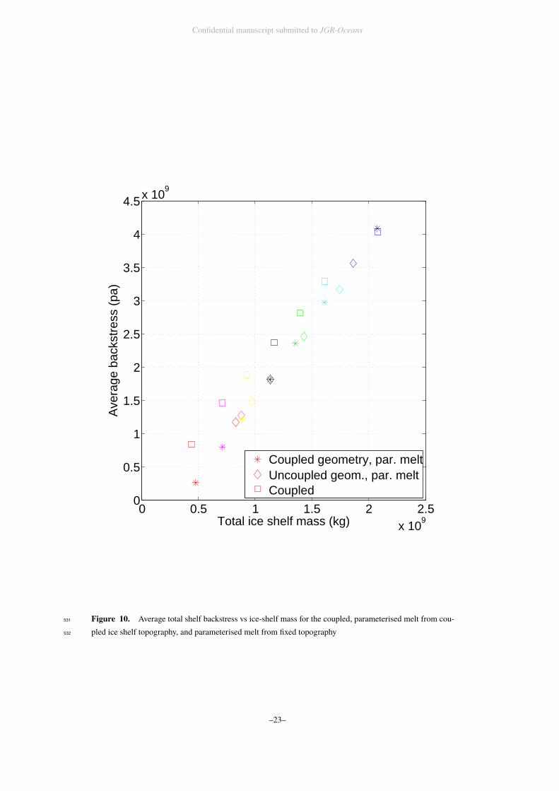
Fig. 10 shows the average backstress, and hence buttressing, of the coupled runs522

as a function of total ice-shelf mass, with warmer runs having both reduced mass and523

buttressing. Note that in reality this reduced buttressing would lead to a speed up of ice524

crossing the grounding line, our model instead has a constant ice influx over the ground-525

ing line. There is a strong correlation between the two, with higher ice-shelf mass leading526

to higher backstress. Raising the pycnocline by 100 m has the effect of reducing back-527

stress by roughly 0.4 × 109 Pa. Whilst the rate of backstress reduction per metre of pycn-528

ocline depth remains constant throughout our runs, as a percentage of total back stress this529

becomes more significant with higher pycnoclines.530

5.4 Comparison of parameterised melt and coupled model533

Finally, we compare our coupled ice shelf–ocean model to an ice only model where534

a typical, depth-dependent melt rate parameterisation [Joughin et al., 2010; Pollard and535

DeConto, 2012; Favier et al., 2014] has been applied. Such a parameterisation typically536

–12–


has no melting for a certain depth close to the surface and then melt rate increasese lin-537

early with depth, reaching a maximum at some depth then maintaining this maximum538

value. We use two different, but similar, methods of parameterising melt for our various539

forcings. In the first, we use an ocean only run with the final steady-state ice-shelf thick-540

ness of the coupled baseline (300) run and apply our seven different forcings. A parame-541

terised melt rate is then derived from the shelf average melt rate (Fig. 9a). In the second542

case, we derive melt rate parameterisations for each forcing from the final, steady-state543

ice-shelf thickness from each respective coupled run (Fig. 9b). This can result in quite544

different parameterisations, namely in the depth at which melting starts and the maximum545

melt rate at depth.546

When using a parameterised, depth-dependent melt rate (Fig. 9c) instead of the fully547

coupled model (Fig. 9d) there is a marked difference in final ice-shelf thickness. Parame-548

terised melt leads to a symmetrical ice shelf with a central ‘bulge’, with no Coriolis driven549

western thinning. This is in direct contrast to the coupled model, which preferentially550

thins the western side of the ice shelf due to Coriolis driven flow.551

Parameterised melt runs also show a strong correlation between ice-shelf mass and552

backstress. However, for a given ice-shelf mass, parameterised runs have less backstress553

then coupled runs. In the baseline case, parameterised melt gives a backstress of roughly554

75% of the coupled run, with the percentage difference growing greater in cases with555

higher melting. This difference is due to the parameterised runs having characteristic ice-556

shelf topography with relatively thin sides and a thicker middle when compared to cou-557

pled runs. As backstress is predominately determined by ice-shelf mass along the margins558

of the ice shelf this leads to a lower backstress for a given ice-shelf mass. In the coldest559

case there is a convergence of the coupled and parameterised runs, as the steady-state cold560

ice-shelf thickness mostly resembles that of a parameetrised melt run. Parameterised melt561

runs using coupled geometry as opposed to uncoupled geometry tend to better reproduce562

the steady-state ice-shelf mass seen in coupled runs, whilst backstress tends to be better563

reproduced by using the uncoupled geometry runs. However, this is mostly because using564

uncoupled geometry for the melt rate leads to a relatively greater ice-shelf mass than the565

coupled geometry, helping to compensate for the general reduction in backstress seen in566

parameterised melt runs.567

6 Discussion568

We have presented here the first truly synchronous coupled ice shelf–ocean model.569

Compared to the previous asynchronous and discontinuous approaches there is no loss of570

information due to model restarts; the model is fully conservative of mass, heat and salt.571

The model can also respond to forcings that vary on a much quicker time-scale than some572

previous approaches. By using the same ocean and ice grid we eliminate the need for av-573

eraging and smoothing of the melt rate. This all combines to allow the model to be ef-574

fectively used in larger scale GCMs. The model is being further developed to incorporate575

a moving grounding line that will allow study of the full ice–ocean system. Large scale576

calving events, such as the detached iceberg in the warm case, could also be investigated577

with the addition of a proper calving model.578

Coupled simulations for a range of pycnocline depths show the ice shelf progres-579

sively thinning on the western boundary, with Coriolis driven flow forming a melt driven580

channel. This asymmetry in ice-shelf topography becomes more pronounced with in-581

creased melting. This is in direct contrast to uncoupled runs with parameterised melt,582

which tend to be symmetrical with relatively thin sides with a thicker central ‘bulge’. As583

a direct result of this, when comparing coupled runs to parameterised melt runs there is584

a significant (roughly 30% in the baseline (300) case) difference in backstress for a given585

ice-shelf mass. Parameterising melt from coupled geometry does give a slightly better in-586

dication of ice-shelf mass than using uncoupled geometry, but as this can only be achieved587

–13–


by running a coupled model, it defeats the point of using parameterised melting in the first588

place.589

The main problem with parameterised melt rates is that, by choosing a depth at590

which melt rates tend to zero, the minimum thickness of the ice shelf is being arbitrarily591

forced. As backstress, and hence buttressing, is strongly dependent upon ice-shelf thick-592

ness this can lead to inaccurate estimates of buttressing change in response to climate593

forcing. To make the issue of using parameterised melting even trickier, the maximum594

melt rate for each of our forcings was found to be different, despite using the same max-595

imum temperature (albeit with a differing position of the pycnocline) in each case. This596

means that, even if ice shelf melt-rate has been successfully parameterised with a given597

pycnocline position, the effect of moving the pycnocline upon melt rate is not the same as598

simply moving the depth of maximum melt rate in the parameterisation. The slope of the599

ice shelf arising from melting affects the melting itself due to a change in the calculation600

of u∗.601

There is no reason why our approach to synchronous coupling could not be used602

with other models. For example, the implementation of ice shelves in NEMO (Nucleus603

for European Modeling of the Ocean) [Mathiot et al., 2017] uses the same pressure load-604

ing method of Losch [2008] which, in combination with a non-linear free surface, forms605

the basis of our synchronous coupling approach. In addition to our synchronous coupling606

approach, the changes made to the boundary layer used in melt rate calculations (which607

greatly reduce, but do not eliminate, the ‘stripy’ melt rates common to z level models)608

could be used in other z level models. As these changes are completely independent of609

the coupling process they can freely be used in uncoupled simulations. Finally, the method610

of model remeshing described here is, with some adjustment of the code, applicable to a611

number of cases involving a moving boundary between two media; for example sea ice612

formation or sediment deposition and erosion.613

7 Conclusions614

1) The first fully synchronous, fully coupled ice shelf–ocean model has been devel-615

oped using the MITgcm. Unlike previous asynchronous and discontinuous methods, our616

approach is fully conservative of heat, salt and mass, making it ideal for use with GCMs.617

2) Coupled simulations shows a characteristic steady-state ice-shelf topography with618

asymmetric thinning focussed on the western boundary due to Coriolis driven flow. In619

contrast, using an ice model with parameterised melting leads to symmetric ice-shelf to-620

pography with relatively thin sides and a thick central ‘bulge’. This leads parameterised621

melting simulations to underestimate ice shelf buttressing for a given ice shelf mass.622

3) Parameterised melt rate profiles arbitarily impose a minimum ice shelf thickness623

by means of a minimum depth for melting. The correct thickness of the ice shelf can only624

be found with a coupled model, defeating the point of using parameterised melting in the625

first place.626

4) The maximum melt rate for each of our forcings was found to be different, de-627

spite using the same maximum temperature. The effect of moving the pycnocline upon628

melt rate is not the same as simply changing the thickness of maximum melt rate in the629

parameterisation.630

–14–


(a) (b)

R

ƞ

Ice shelf

Ocean

Bv2

Bv1

BχΔz

Δz

zz=zsurf

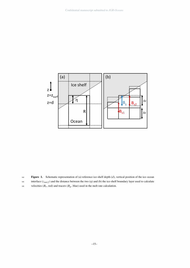
z=d

Figure 1. Schematic representation of (a) reference ice-shelf depth (d), vertical position of the ice–oceaninterface (zsur f ) and the distance between the two (η) and (b) the ice-shelf boundary layer used to calculatevelocities (Bv , red) and tracers (Bχ , blue) used in the melt rate calculation.

163

164

165

–15–


i=1 i=2 i=3 i=1 i=2 i=3i=1 i=2 i=3

k=1

k=2

k=3

k=1

k=2

k=3 k=3

k=2

k=1

hcΔz hcΔz hcΔz

hcΔz

ΔzΔz Δz

(a) (b) (c)

Figure 2. Schematic representation of hc and cells in (a) a ’normal‘ case (b) a cell with hc > hmax just be-fore a model remesh check and (c) the same cell just after a model remesh has occurred.

275

276

Ice Shelf

Ice shelf Ocean

160 km

60 km

60 km

1100 m

Southern boundary,ice enters domain

Northern boundary,ocean temperature and salinity restored

Figure 3. Schematic representation of model domain.360

–16–


−2 −1 0 1 2−1100

−1000

−900

−800

−700

−600

−500

−400

−300

−200

−100

0

Dep

th (

m)

Temperature oC

a

33.5 34 34.5 35 35.5−1100

−1000

−900

−800

−700

−600

−500

−400

−300

−200

−100

0D

epth

(m

)

Salinity (psu)

b

Hot100200300400500Cold

Figure 4. (Initial and restoring temperature (a) and salinity (b) profiles for the seven temperature variationruns.

379

380

–17–


0 10 20 30 40 50time (yrs)

0

0.2

0.4

0.6

0.8

r.m

.s. h

dif

f

0.025y time step0.1y time step

Figure 5. (Comparison of split ice-model time stepping and conventional time stepping.418

–18–


0

20

40

600

20

40

60

−800

−600

−400

−200

0a

0

20

40

600

20

40

60

−800

−600

−400

−200

0b

0

20

40

600

20

40

60

−800

−600

−400

−200

0c

0

20

40

600

20

40

60

−800

−600

−400

−200

0d

Figure 6. Evolution of ice-shelf depth for initial (a), year 5 (b), year 13 (c) and year 60 (d) in the baseline,300 m case.

439

440

–19–


Baseline (300)

Year 10.2 m/s

−900

−800

−700

−600

−500

−400

−300

−200

−100

0

Year 50.2 m/s

Year 130.2 m/s

Year 600.2 m/s

Hot

Year 10.2 m/s

Year 50.2 m/s

Year 130.2 m/s

Year 600.2 m/s

Cold

Year 10.2 m/s

Year 50.2 m/s

Year 130.2 m/s

Year 600.2 m/s

Figure 7. Ice thickness (colours) with ice-shelf boundary layer velocities (arrows) for the baseline (300)),warm and cold forcings at year 1, year 5, year 13 and year 60.

456

457

–20–


Melt rate (m/a)

Year 1

0

0.005

0.01

0.015

0.02

0.025

0.03Thermal driving ( °C)

Year 1

0

0.5

1

1.5

2

2.5u* (m/s)

Year 1

0

1

7

20

43

80

130

Year 5 Year 5 Year 5



Figure 8. Melt rate, thermal driving and u∗ for the baseline coupled run at years 1, 5, 13, and 60.484

–21–


0 50 100 150

−1000

−800

−600

−400

−200

0

Melt rate (m/a)

Dep

th (

m)

b

Hot100200300400500Cold

0 50 100 150

−1000

−800

−600

−400

−200

0

Melt rate (m/a)

Dep

th (

m)

a

Hot100200300400500Cold

Coupled 300

d −1000

−800

−600

−400

−200

0Parm. Melt 300

c −1000

−800

−600

−400

−200

0

Figure 9. Depth averaged mean melt rates (dashed line) and parameterised melt rate (solid line) for thetemperature varying cases using steady-state ice-shelf thickness from the coupled model for each individualforcing (a), depth averaged mean melt rates (dashed line) and parameterised melt rate (solid line) for thetemperature varying cases using steady-state ice-shelf thickness from the 300 m coupled model (b), Final,steady-state ice-shelf thickness for the coupled, baseline case (c) and the parameterised melt, baseline (300)case (d).

516

517

518

519

520

521

–22–


0 0.5 1 1.5 2 2.5x 10

9

0

0.5

1

1.5

2

2.5

3

3.5

4

4.5x 109

Total ice shelf mass (kg)

Ave

rage

bac

kstr

ess

(pa)

Coupled geometry, par. meltUncoupled geom., par. meltCoupled

Figure 10. Average total shelf backstress vs ice-shelf mass for the coupled, parameterised melt from cou-pled ice shelf topography, and parameterised melt from fixed topography

531

532

–23–


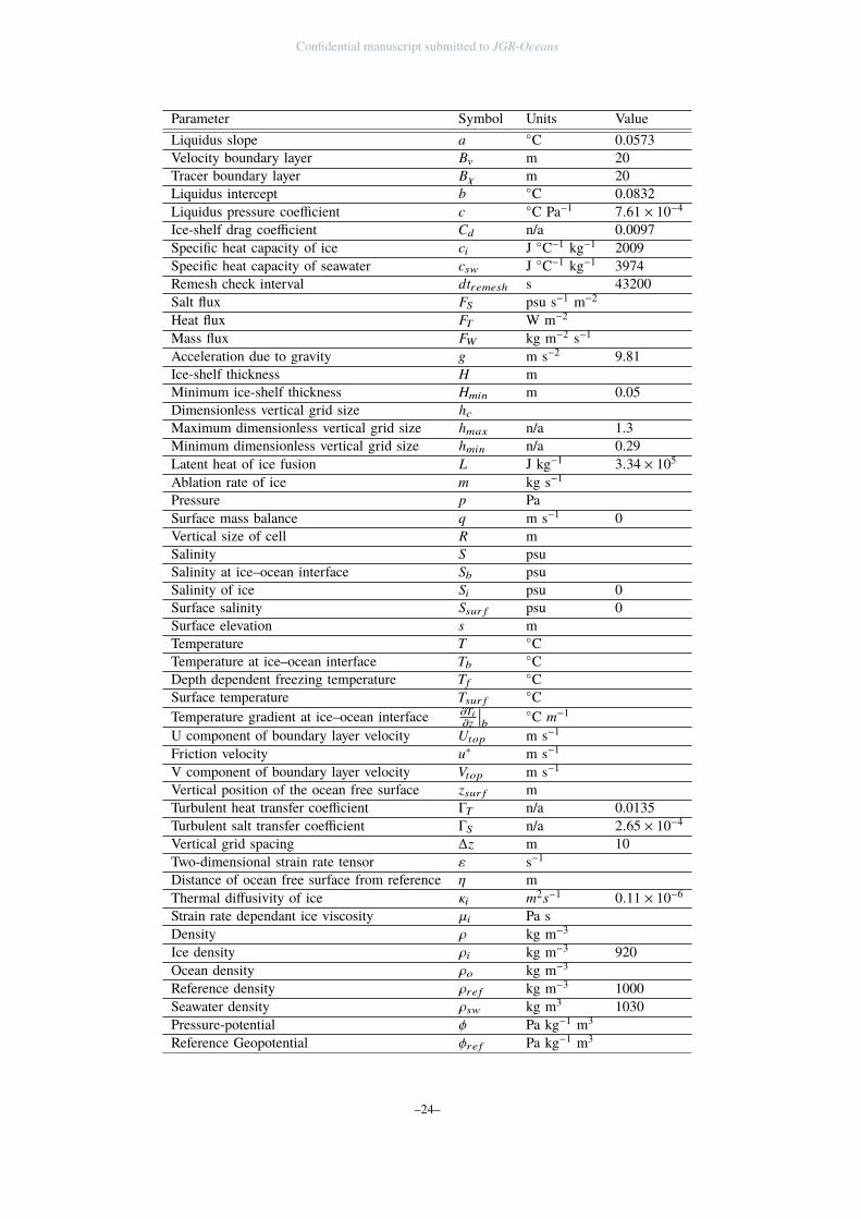
Parameter Symbol Units ValueLiquidus slope a ◦C 0.0573Velocity boundary layer Bv m 20Tracer boundary layer Bχ m 20Liquidus intercept b ◦C 0.0832Liquidus pressure coefficient c ◦C Pa−1 7.61 × 10−4

Ice-shelf drag coefficient Cd n/a 0.0097Specific heat capacity of ice ci J ◦C−1 kg−1 2009Specific heat capacity of seawater csw J ◦C−1 kg−1 3974Remesh check interval dtremesh s 43200Salt flux FS psu s−1 m−2

Heat flux FT W m−2

Mass flux FW kg m−2 s−1

Acceleration due to gravity g m s−2 9.81Ice-shelf thickness H mMinimum ice-shelf thickness Hmin m 0.05Dimensionless vertical grid size hcMaximum dimensionless vertical grid size hmax n/a 1.3Minimum dimensionless vertical grid size hmin n/a 0.29Latent heat of ice fusion L J kg−1 3.34 × 105

Ablation rate of ice m kg s−1

Pressure p PaSurface mass balance q m s−1 0Vertical size of cell R mSalinity S psuSalinity at ice–ocean interface Sb psuSalinity of ice Si psu 0Surface salinity Ssur f psu 0Surface elevation s mTemperature T ◦CTemperature at ice–ocean interface Tb

◦CDepth dependent freezing temperature Tf

◦CSurface temperature Tsur f

◦CTemperature gradient at ice–ocean interface ∂Ti

∂z

��b

◦C m−1

U component of boundary layer velocity Utop m s−1

Friction velocity u∗ m s−1

V component of boundary layer velocity Vtop m s−1

Vertical position of the ocean free surface zsur f mTurbulent heat transfer coefficient ΓT n/a 0.0135Turbulent salt transfer coefficient ΓS n/a 2.65 × 10−4

Vertical grid spacing ∆z m 10Two-dimensional strain rate tensor ε s−1

Distance of ocean free surface from reference η mThermal diffusivity of ice κi m2s−1 0.11 × 10−6

Strain rate dependant ice viscosity µi Pa sDensity ρ kg m−3

Ice density ρi kg m−3 920Ocean density ρo kg m−3

Reference density ρre f kg m−3 1000Seawater density ρsw kg m3 1030Pressure-potential φ Pa kg−1 m3

Reference Geopotential φre f Pa kg−1 m3

–24–


Geopotential at reference ice-shelf depth φd Pa kg−1 m3

Table 1: Model parameters and constants

–25–


Acknowledgments631

This work was supported by the UK Natural Environment Research Council under grant632

NE/M003590/1633

–26–

References634

Adcroft, A., C. Hill, and J. Marshall (1997), Representation of topography by shaved cells635

in a height coordinate ocean model, Monthly Weather Review, 125(9), 2293–2315, doi:636

10.1175/1520-0493(1997)125<2293:ROTBSC>2.0.CO;2.637

Campin, J.-M., A. Adcroft, C. Hill, and J. Marshall (2004), Conservation of prop-638

erties in a free-surface model, Ocean Modelling, 6(3âĂŞ4), 221 – 244, doi:639

http://doi.org/10.1016/S1463-5003(03)00009-X.640

De Rydt, J., and G. H. Gudmundsson (2016), Coupled ice shelf-ocean modeling and com-641

plex grounding line retreat from a seabed ridge, Journal of Geophysical Research: Earth642

Surface, 121(5), 865–880, doi:10.1002/2015JF003791, 2015JF003791.643

De Rydt, J., P. R. Holland, P. Dutrieux, and A. Jenkins (2014), Geometric and oceano-644

graphic controls on melting beneath Pine Island Glacier, Journal of Geophysical Re-645

search: Oceans, 119(4), 2420–2438, doi:10.1002/2013JC009513.646

Depoorter, M. A., J. L. Bamber, J. A. Griggs, J. T. M. Lenaerts, S. R. M. Ligtenberg,647

M. R. van den Broeke, and G. Moholdt (2013), Calving fluxes and basal melt rates of648

Antarctic ice shelves, Nature, 502, 89–92, doi:10.1038/nature12567.649

Dupont, T., and R. Alley (2005), Assessment of the importance of ice-shelf buttressing to650

ice-sheet flow, Geophysical Research Letters, 32(4).651

Dutrieux, P., J. De Rydt, A. Jenkins, P. R. Holland, H. K. Ha, S. H. Lee, E. J. Steig,652

Q. Ding, E. P. Abrahamsen, and M. Schröder (2014), Strong sensitivity of Pine Is-653

land Ice-Shelf melting to climatic variability, Science, 343(6167), 174–178, doi:654

10.1126/science.1244341.655

Favier, L., G. Durand, S. L. Cornford, H. G. Gudmundsson, O. Gagliardi, F. Gillet-656

Chaulet, T. Zwinger, A. J. Payne, and A. M. L. Brocq (2014), Retreat of Pine Island657

Glacier controlled by marine ice-sheet instability, Nature Climate Change, 4(2), 336 –658

348, doi:10.1038/nclimate2094.659

Gladish, C. V., D. M. Holland, P. R. Holland, and S. F. Price (2012), Ice-shelf basal chan-660

nels in a coupled ice/ocean model, Journal of Glaciology, 58(212), 1227–1244, doi:661

doi:10.3189/2012JoG12J003.662

Goldberg, D., and P. Heimbach (2013), Parameter and state estimation with a time-663

dependent adjoint marine ice sheet model, The Cryosphere, 7(6), 1659–1678.664

Goldberg, D. N., C. M. Little, O. V. Sergienko, A. Gnanadesikan, R. Hallberg, and665

M. Oppenheimer (2012a), Investigation of land ice-ocean interaction with a fully cou-666

pled ice-ocean model: 1. model description and behavior, Journal of Geophysical Re-667

search: Earth Surface, 117(F2), n/a–n/a, doi:10.1029/2011JF002246, f02037.668

Goldberg, D. N., C. M. Little, O. V. Sergienko, A. Gnanadesikan, R. Hallberg, and669

M. Oppenheimer (2012b), Investigation of land ice-ocean interaction with a fully cou-670

pled ice-ocean model: 2. sensitivity to external forcings, Journal of Geophysical Re-671

search: Earth Surface, 117(F2), n/a–n/a, doi:10.1029/2011JF002247, f02038.672

Greenbaum, J. S., D. D. Blankenship, D. A. Young, T. G. Richter, J. L. Roberts, A. R. A.673

Aitken, B. Legresy, D. M. Schroeder, R. C. Warner, T. D. van Ommen, and M. J. Sie-674

gart (2015), Ocean access to a cavity beneath Totten Glacier in East Antarctica, Nature675

Geosci, 8, 294–298, doi:10.1038/ngeo2388.676

Jacobs, S., H. H. Helmer, C. S. M. Doake, A. Jenkins, and R. M. Frolich (1992), Melting677

of ice shelves and the mass balance of Antarctica, Journal of Glaciology, 38(130).678

Jacobs, S. S., H. H. Hellmer, and A. Jenkins (1996), Antarctic Ice Sheet melt-679

ing in the southeast Pacific, Geophysical Research Letters, 23(9), 957–960, doi:680

10.1029/96GL00723.681

Jenkins, A., H. H. Hellmer, and D. M. Holland (2001), The role of meltwater ad-682

vection in the formulation of conservative boundary conditions at an iceâĂŞocean683

interface, Journal of Physical Oceanography, 31(1), 285–296, doi:10.1175/1520-684

0485(2001)031<0285:TROMAI>2.0.CO;2.685


Jenkins, A., P. Dutrieux, S. S. Jacobs, S. D. McPhail, J. R. Perrett, A. T. Webb, and686

D. White (2010), Observations beneath Pine Island Glacier in West Antarctica and im-687

plications for its retreat, Nature Geoscience, 3, 468–472, doi:10.1038/ngeo890.688

Joughin, I., B. E. Smith, and D. M. Holland (2010), Sensitivity of 21st century sea level689

to ocean-induced thinning of pine island glacier, antarctica, Geophysical Research Let-690

ters, 37(20), n/a–n/a, doi:10.1029/2010GL044819.691

Joughin, I., R. B. Alley, and D. M. Holland (2012), Ice-sheet response to oceanic forcing,692

Science, 338(6111), 1172–1176, doi:10.1126/science.1226481.693

Losch, M. (2008), Modeling ice shelf cavities in a z coordinate ocean general cir-694

culation model, Journal of Geophysical Research: Oceans, 113(C8), n/a–n/a, doi:695

10.1029/2007JC004368, c08043.696

MacAyeal, D. R. (1989), Large-scale ice flow over a viscous basal sediment: Theory and697

application to ice stream b, antarctica, Journal of Geophysical Research: Solid Earth,698

94(B4), 4071–4087, doi:10.1029/JB094iB04p04071.699

Marshall, J., C. Hill, L. Perelman, and A. Adcroft (1997), Hydrostatic, quasi-hydrostatic,700

and nonhydrostatic ocean modeling, Journal of Geophysical Research: Oceans, 102(C3),701

5733–5752, doi:10.1029/96JC02776.702

Mathiot, P., A. Jenkins, C. Harris, and G. Madec (2017), Explicit and parametrised rep-703

resentation of under ice shelf seas in a z∗ coordinate ocean model, Geoscientific Model704

Development Discussions, 2017, 1–43, doi:10.5194/gmd-2017-37.705

Pattyn, F., and G. Durand (2013), Why marine ice sheet model predictions may diverge706

in estimating future sea level rise, Geophysical Research Letters, 40(16), 4316–4320,707

doi:10.1002/grl.50824.708

Petty, A. A., D. L. Feltham, and P. R. Holland (2013), Impact of atmospheric forcing on709

antarctic continental shelf water masses, Journal of Physical Oceanography, 43(5), 920–710

940, doi:10.1175/JPO-D-12-0172.1.711

Pollard, D., and R. M. DeConto (2012), Description of a hybrid ice sheet-shelf model,712

and application to Antarctica, Geoscientific Model Development, 5(5), 1273–1295, doi:713

10.5194/gmd-5-1273-2012.714

Scambos, T. A., J. A. Bohlander, C. A. Shuman, and P. Skvarca (2004), Glacier accel-715

eration and thinning after ice shelf collapse in the Larsen B embayment, Antarctica,716

Geophysical Research Letters, 31.717

Seroussi, H., Y. Nakayama, E. Larour, D. Menemenlis, M. Morlighem, E. Rignot, and718

A. Khazendar (2017), Continued retreat of thwaites glacier, west antarctica, controlled719

by bed topography and ocean circulation, Geophysical Research Letters, pp. n/a–n/a,720

doi:10.1002/2017GL072910, 2017GL072910.721

Shepherd, A., D. Wingham, and E. Rignot (2004), Warm ocean is eroding West Antarctic722

Ice Sheet, Geophysical Research Letters, 31(23), n/a–n/a, doi:10.1029/2004GL021106,723

l23402.724

Silvano, A., S. R. Rintoul, and L. Herraiz-Borreguero (2016), Ocean-ice shelf interaction725

in east antarctica, Oceanography, 29.726

Thomas, R. H. (1979), The dynamics of marine ice sheets, Journal of Glaciology, 24(90),727

167–177, doi:doi:10.3198/1979JoG24-90-167-177.728

Thomas, R. H., T. J. O. Sanderson, and K. E. Rose (1979), Effect of climatic warming on729

the West Antarctic Ice Sheet, Nature, 277, 355–358, doi:doi:10.1038/277355a0.730

Walker, D. P., M. A. Brandon, A. Jenkins, J. T. Allen, J. A. Dowdeswell, and J. Evans731

(2007), Oceanic heat transport onto the amundsen sea shelf through a submarine glacial732

trough, Geophysical Research Letters, 34(2), n/a–n/a, doi:10.1029/2006GL028154,733

l02602.734

Walker, R. T., and D. M. Holland (2007), A two-dimensional coupled model735

for ice shelfâĂŞocean interaction, Ocean Modelling, 17(2), 123 – 139, doi:736

https://doi.org/10.1016/j.ocemod.2007.01.001.737

–28–

Northumbria Research Linknrl.northumbria.ac.uk/33708/1/Ocean-forced ice... · Northumbria Research...

Documents

Transcript of Northumbria Research Linknrl.northumbria.ac.uk/33708/1/Ocean-forced ice... · Northumbria Research...