norske recom practice.pdf
46
RECOMMENDED PRACTICE DET NORSKE VERITAS DNV-RP-F105 FREE SPANNING PIPELINES FEBRUARY 2006
-
Upload
jonathan-gardner -
Category
Documents
-
view
48 -
download
0
Transcript of norske recom practice.pdf
RECOMMENDED PRACTICE
DET NORSKE VERITAS
DNV-RP-F105
FREE SPANNING PIPELINES
FEBRUARY 2006

FOREWORDDET NORSKE VERITAS (DNV) is an autonomous and independent foundation with the objectives of safeguarding life, prop-erty and the environment, at sea and onshore. DNV undertakes classification, certification, and other verification and consultancyservices relating to quality of ships, offshore units and installations, and onshore industries worldwide, and carries out researchin relation to these functions.DNV Offshore Codes consist of a three level hierarchy of documents:— Offshore Service Specifications. Provide principles and procedures of DNV classification, certification, verification and con-
sultancy services.— Offshore Standards. Provide technical provisions and acceptance criteria for general use by the offshore industry as well as
the technical basis for DNV offshore services.— Recommended Practices. Provide proven technology and sound engineering practice as well as guidance for the higher level
Offshore Service Specifications and Offshore Standards.DNV Offshore Codes are offered within the following areas:A) Qualification, Quality and Safety MethodologyB) Materials TechnologyC) StructuresD) SystemsE) Special FacilitiesF) Pipelines and RisersG) Asset OperationH) Marine OperationsJ) Wind Turbines
Amendments and Corrections This document is valid until superseded by a new revision. Minor amendments and corrections will be published in a separatedocument normally updated twice per year (April and October). For a complete listing of the changes, see the “Amendments and Corrections” document located at: http://www.dnv.com/technologyservices/, “Offshore Rules & Standards”, “Viewing Area”.
The electronic web-versions of the DNV Offshore Codes will be regularly updated to include these amendments and corrections.Comments may be sent by e-mail to [email protected] subscription orders or information about subscription terms, please use [email protected] information about DNV services, research and publications can be found at http://www.dnv.com, or can be obtained from DNV, Veritas-veien 1, NO-1322 Høvik, Norway; Tel +47 67 57 99 00, Fax +47 67 57 99 11.
© Det Norske Veritas. All rights reserved. No part of this publication may be reproduced or transmitted in any form or by any means, including pho-tocopying and recording, without the prior written consent of Det Norske Veritas.
Computer Typesetting (FM+SGML) by Det Norske Veritas.Printed in Norway
If any person suffers loss or damage which is proved to have been caused by any negligent act or omission of Det Norske Veritas, then Det Norske Veritas shall pay compensation to such personfor his proved direct loss or damage. However, the compensation shall not exceed an amount equal to ten times the fee charged for the service in question, provided that the maximum compen-sation shall never exceed USD 2 million.In this provision "Det Norske Veritas" shall mean the Foundation Det Norske Veritas as well as all its subsidiaries, directors, officers, employees, agents and any other acting on behalf of DetNorske Veritas.
Recommended Practice DNV-RP-F105, February 2006 Introduction – Page 3
Relationship to Rules under preparation Parts of this Recommended Practice should be read in conjunc-tion with the following two documents:
— DNV-RP-F110 "Global Buckling of Pipelines", and— DNV-RP-C205 - "Environmental Conditions and
Environmental Loads".
However, these two documents are currently under preparationat DNV. Readers are requested to contact:RP-F110: Leif Collberg, TNCNO714, Det Norske Veritas,Veritasveien 1, N-1322 Høvik, mailto: [email protected]: Arne Nestegaard, TNCNO785, Det Norske Veritas,Veritasveien 1, N-1322 Høvik, mailto: [email protected] more information, if required.
Motives The existing design code, DNV-RP-F105 for "Free SpanningPipelines" from March 2002, can be effectively applied to dealwith both single and multiple spans vibrating predominantly ina single mode. In the case where there is a combination of longspans and high currents, not only does the fundamental eigenmodes become activated, but also the higher modes. Such amultimode response is not prohibited by the design code.However, no detailed guidance is provided in the present Rec-ommended Practice (RP) about the fatigue damage from mul-timode vibrations. During the Ormen Lange project a strong focus was put on de-sign procedures for long free spans in order to make thisproject feasible and in order to save seabed intervention costs.A relatively large R&D project on free span vortex-induced vi-brations (VIV) was performed. The results of this project wassynthesised into a project specific guideline issued by DNV,concerning the calculation procedures and design acceptancecriteria for long free span with multi-mode response.The main objective of this proposal is to include the experienc-es gained from the Ormen Lange Project regarding multi-modeand multi-span response and incorporate the latest R&D workrelating to Free Spanning Pipelines. This proposal has beenworked out through a JIP with Hydro and Statoil. In addition
to the multi-mode response aspects, a general update and revi-sion of the DNV-RP-F105 has been performed, based on feed-back and experience from several projects and users.
Main changesThe most important changes in this update are:
— Computational procedure for multi-mode analysis, selec-tion of vibration modes and combination of stresses.
— Guidance on mitigation measures for vortex-induced vi-brations.
— Ultimate limit state criteria (over-stress) updated.— Recalibrated safety factors.— Detailed calculation procedure for pipe-soil interaction.— Practical guidance on various aspects based on project ex-
perience from several sources.— Update of response models for vortex-induced vibrations
based on available test results.— Clarified limitations and range of application.— Added mass modification during cross-flow vibrations.
This update strengthens the position of this RP as the state-of-the-art document for free spanning pipelines. It allows longerspans to be accepted as detailed calculation procedures formultiple mode response is given.
Acknowledgement:The following companies are gratefully acknowledged fortheir contributions to this Recommended Practice:
DHIHydroReinertsenStatoilSnamprogetti
DNV is grateful for the valuable co-operations and discussionswith the individual personnel of these companies.The multispan and multi-mode studies were funded by the Or-men Lange license group.Hydro and its license partners BP, Exxon, Petoro, Shell andStatoil are acknowledged for the permission to use these re-sults.
DET NORSKE VERITAS

Recommended Practice DNV-RP-F105, February 2006Page 4 – Introduction
DET NORSKE VERITAS
, Recommended Practice DNV-RP-F105, February 2006Page 5
CONTENTS
1. GENERAL .............................................................. 71.1 Introduction .............................................................71.2 Objective...................................................................71.3 Scope and application .............................................71.4 Extending the application scope of this RP ..........81.5 Safety philosophy.....................................................81.6 Free span morphological classification..................81.7 Free span response classification ...........................91.8 Free span response behaviour ................................91.9 Flow regimes ..........................................................101.10 VIV assessment methodologies.............................101.11 Relationship to other Rules ..................................101.12 Definitions ..............................................................111.13 Abbreviations.........................................................111.14 Symbols...................................................................11
2. DESIGN CRITERIA............................................ 132.1 General ...................................................................132.2 Non-stationarity of spans ......................................142.3 Screening fatigue criteria......................................152.4 Fatigue criterion ....................................................152.5 ULS criterion .........................................................162.6 Safety factors..........................................................18
3. ENVIRONMENTAL CONDITIONS................. 193.1 General ...................................................................193.2 Current conditions ................................................193.3 Short-term wave conditions..................................203.4 Reduction functions...............................................213.5 Long-term environmental modelling...................223.6 Return period values .............................................22
4. RESPONSE MODELS......................................... 234.1 General ...................................................................234.2 Marginal fatigue life capacity...............................234.3 In-line response model .........................................24
4.4 Cross-flow response model ................................... 254.5 Added mass coefficient model .............................. 27
5. FORCE MODEL.................................................. 275.1 General ................................................................... 275.2 FD solution for in-line direction .......................... 275.3 Simplified fatigue assessment............................... 295.4 Force coefficients................................................... 29
6. STRUCTURAL ANALYSIS............................... 306.1 General ................................................................... 306.2 Structural modelling ............................................. 306.3 Functional loads .................................................... 316.4 Static analysis ........................................................ 316.5 Eigen value analyses ............................................. 326.6 FEM based response quantities ........................... 326.7 Approximate response quantities ........................ 326.8 Approximate response quantities for higher
order modes of isolated single spans ................... 346.9 Added mass............................................................ 34
7. PIPE-SOIL INTERACTION .............................. 347.1 General ................................................................... 347.2 Modelling of pipe-soil interaction ....................... 357.3 Soil damping .......................................................... 357.4 Penetration and soil stiffness................................ 357.5 Artificial supports ................................................. 38
8. REFERENCES..................................................... 38
APP. A MULTI-MODE RESPONSE............................. 39
APP. B VIV MITIGATION............................................ 42
APP. C VIV IN OTHER OFFSHORE APPLICATIONS ............................................................... 43
APP. D DETAILED ASSESSMENT OF PIPE-SOIL INTERACTION................................................................. 44
DET NORSKE VERITAS

Recommended Practice DNV-RP-F105, February 2006 ,Page 6
DET NORSKE VERITAS
Recommended Practice DNV-RP-F105, February 2006Page 7
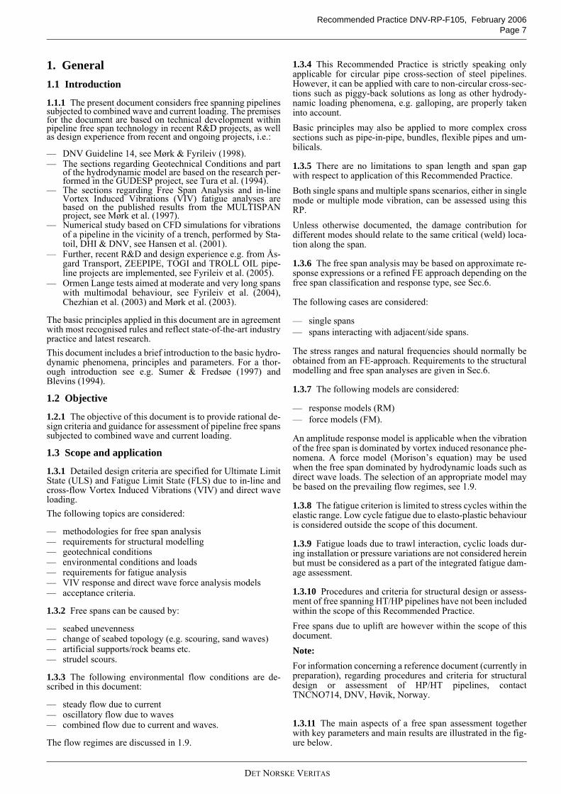
1. General1.1 Introduction
1.1.1 The present document considers free spanning pipelinessubjected to combined wave and current loading. The premisesfor the document are based on technical development withinpipeline free span technology in recent R&D projects, as wellas design experience from recent and ongoing projects, i.e.:
— DNV Guideline 14, see Mørk & Fyrileiv (1998).— The sections regarding Geotechnical Conditions and part
of the hydrodynamic model are based on the research per-formed in the GUDESP project, see Tura et al. (1994).
— The sections regarding Free Span Analysis and in-lineVortex Induced Vibrations (VIV) fatigue analyses arebased on the published results from the MULTISPANproject, see Mørk et al. (1997).
— Numerical study based on CFD simulations for vibrationsof a pipeline in the vicinity of a trench, performed by Sta-toil, DHI & DNV, see Hansen et al. (2001).
— Further, recent R&D and design experience e.g. from Ås-gard Transport, ZEEPIPE, TOGI and TROLL OIL pipe-line projects are implemented, see Fyrileiv et al. (2005).
— Ormen Lange tests aimed at moderate and very long spanswith multimodal behaviour, see Fyrileiv et al. (2004),Chezhian et al. (2003) and Mørk et al. (2003).
The basic principles applied in this document are in agreementwith most recognised rules and reflect state-of-the-art industrypractice and latest research.This document includes a brief introduction to the basic hydro-dynamic phenomena, principles and parameters. For a thor-ough introduction see e.g. Sumer & Fredsøe (1997) andBlevins (1994).
1.2 Objective
1.2.1 The objective of this document is to provide rational de-sign criteria and guidance for assessment of pipeline free spanssubjected to combined wave and current loading.
1.3 Scope and application
1.3.1 Detailed design criteria are specified for Ultimate LimitState (ULS) and Fatigue Limit State (FLS) due to in-line andcross-flow Vortex Induced Vibrations (VIV) and direct waveloading. The following topics are considered:
— methodologies for free span analysis— requirements for structural modelling— geotechnical conditions — environmental conditions and loads— requirements for fatigue analysis— VIV response and direct wave force analysis models— acceptance criteria.
1.3.2 Free spans can be caused by:
— seabed unevenness— change of seabed topology (e.g. scouring, sand waves)— artificial supports/rock beams etc.— strudel scours.
1.3.3 The following environmental flow conditions are de-scribed in this document:
— steady flow due to current— oscillatory flow due to waves— combined flow due to current and waves.
The flow regimes are discussed in 1.9.
1.3.4 This Recommended Practice is strictly speaking onlyapplicable for circular pipe cross-section of steel pipelines.However, it can be applied with care to non-circular cross-sec-tions such as piggy-back solutions as long as other hydrody-namic loading phenomena, e.g. galloping, are properly takeninto account.Basic principles may also be applied to more complex crosssections such as pipe-in-pipe, bundles, flexible pipes and um-bilicals.
1.3.5 There are no limitations to span length and span gapwith respect to application of this Recommended Practice.Both single spans and multiple spans scenarios, either in singlemode or multiple mode vibration, can be assessed using thisRP. Unless otherwise documented, the damage contribution fordifferent modes should relate to the same critical (weld) loca-tion along the span.
1.3.6 The free span analysis may be based on approximate re-sponse expressions or a refined FE approach depending on thefree span classification and response type, see Sec.6.
The following cases are considered:
— single spans— spans interacting with adjacent/side spans.
The stress ranges and natural frequencies should normally beobtained from an FE-approach. Requirements to the structuralmodelling and free span analyses are given in Sec.6.
1.3.7 The following models are considered:
— response models (RM)— force models (FM).
An amplitude response model is applicable when the vibrationof the free span is dominated by vortex induced resonance phe-nomena. A force model (Morison’s equation) may be usedwhen the free span dominated by hydrodynamic loads such asdirect wave loads. The selection of an appropriate model maybe based on the prevailing flow regimes, see 1.9.
1.3.8 The fatigue criterion is limited to stress cycles within theelastic range. Low cycle fatigue due to elasto-plastic behaviouris considered outside the scope of this document.
1.3.9 Fatigue loads due to trawl interaction, cyclic loads dur-ing installation or pressure variations are not considered hereinbut must be considered as a part of the integrated fatigue dam-age assessment.
1.3.10 Procedures and criteria for structural design or assess-ment of free spanning HT/HP pipelines have not been includedwithin the scope of this Recommended Practice.Free spans due to uplift are however within the scope of thisdocument.Note:For information concerning a reference document (currently inpreparation), regarding procedures and criteria for structuraldesign or assessment of HP/HT pipelines, contactTNCNO714, DNV, Høvik, Norway.
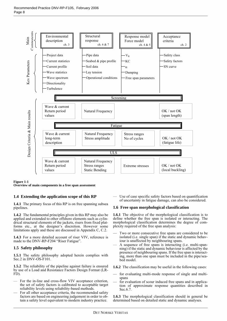
1.3.11 The main aspects of a free span assessment togetherwith key parameters and main results are illustrated in the fig-ure below.
DET NORSKE VERITAS
Recommended Practice DNV-RP-F105, February 2006 Page 8
Figure 1-1Overview of main components in a free span assessment
1.4 Extending the application scope of this RP
1.4.1 The primary focus of this RP is on free spanning subseapipelines.
1.4.2 The fundamental principles given in this RP may also beapplied and extended to other offshore elements such as cylin-drical structural elements of the jackets, risers from fixed plat-forms etc., at the designer’s discretion. However somelimitations apply and these are discussed in Appendix C, C.2.
1.4.3 For a more detailed account of riser VIV, reference ismade to the DNV-RP-F204 “Riser Fatigue”.
1.5 Safety philosophy
1.5.1 The safety philosophy adopted herein complies withSec.2 in DNV-OS-F101.
1.5.2 The reliability of the pipeline against failure is ensuredby use of a Load and Resistance Factors Design Format (LR-FD).
— For the in-line and cross-flow VIV acceptance criterion,the set of safety factors is calibrated to acceptable targetreliability levels using reliability-based methods.
— For all other acceptance criteria, the recommended safetyfactors are based on engineering judgement in order to ob-tain a safety level equivalent to modern industry practice.
— Use of case specific safety factors based on quantificationof uncertainty in fatigue damage, can also be considered.
1.6 Free span morphological classification
1.6.1 The objective of the morphological classification is todefine whether the free span is isolated or interacting. Themorphological classification determines the degree of com-plexity required of the free span analysis:
— Two or more consecutive free spans are considered to beisolated (i.e. single span) if the static and dynamic behav-iour is unaffected by neighbouring spans.
— A sequence of free spans is interacting (i.e. multi-span-ning) if the static and dynamic behaviour is affected by thepresence of neighbouring spans. If the free span is interact-ing, more than one span must be included in the pipe/sea-bed model.
1.6.2 The classification may be useful in the following cases:
— for evaluating multi-mode response of single and multi-spans
— for evaluation of scour induced free spans and in applica-tion of approximate response quantities described inSec.6.7.
1.6.3 The morphological classification should in general bedetermined based on detailed static and dynamic analyses.
Environmentaldescription
ch. 3
Project data
Current statisticsCurrent profile
Wave statisticsWave spectrumDirectionalityTurbulence
Wave & currentReturn periodvalues
Wave & currentlong-termdescription
Screening
Fatigue
ULS
Wave & currentReturn periodvalues
Structuralresponse
ch. 6 & 7
Pipe data
Seabed & pipe profileSoil data
Lay tensionOperational conditions
Natural Frequency
Natural FrequencyStress amplitude
Natural FrequencyStress rangesStatic Bending
Response modelForce model
ch. 4 & 5
VR
KC
α
DampingFree span parameters
Stress rangesNo of cycles
Extreme stresses
Acceptancecriteria
ch. 2
Safety class
Safety factorsSN curve
OK / not OK(span length)
OK / not OK(fatigue life)
OK / not OK(local buckling)
Mai
nC
ompo
nent
sK
ey P
aram
eter
sD
esi g
n C
riter
ia &
Mai
n re
sults
DET NORSKE VERITAS
Recommended Practice DNV-RP-F105, February 2006Page 9
Guidance note:When long segments of the pipeline are analysed in automatedFE analysis tools, certain limitations can arise for identifying in-teracting spans. The following example illustrates the same: Two free spans which are separated by a distance of 1000 m andeach with a span length of about 50 m. The FE analysis estimatesthat some of the response frequencies for these two spans areidentical. Further, due to numerical approximations or due toround off errors, the results may be presented as single mode re-sponse at these two spans, i.e. it is a single interacting mode atthese two spans. However, in reality these two spans are physically separated bya considerable distance, and not interacting. If isolated spans are incorrectly modelled as interacting multi-spans, it may also lead to significant errors in estimating the fa-tigue damage. The fatigue damage is dependent on the unit stressamplitudes, as discussed in Sec.4. The unit stress amplitudes aredependent on the normalised mode shape, which is related to thespan length over which the normalisation is considered. Whenlong multispans are analysed, the normalisation will not be sameas for an isolated single span, within the multi-spanning system.This will in turn lead to errors.Experience has shown that in case of close frequencies for spans,the FE analysis may predict interaction even though the physicaldistance between the spans is quite long. In case of mode shapeswith deflection in spans that seem to be physically well separat-ed, use of appropriate axial pipe-soil stiffness and/or local re-straints in between the spans should be considered to separateindividual modes.Hence, caution should be exercised when using automated FEtools for identifying interacting spans.
---e-n-d---of---G-u-i-d-a-n-c-e---n-o-t-e---
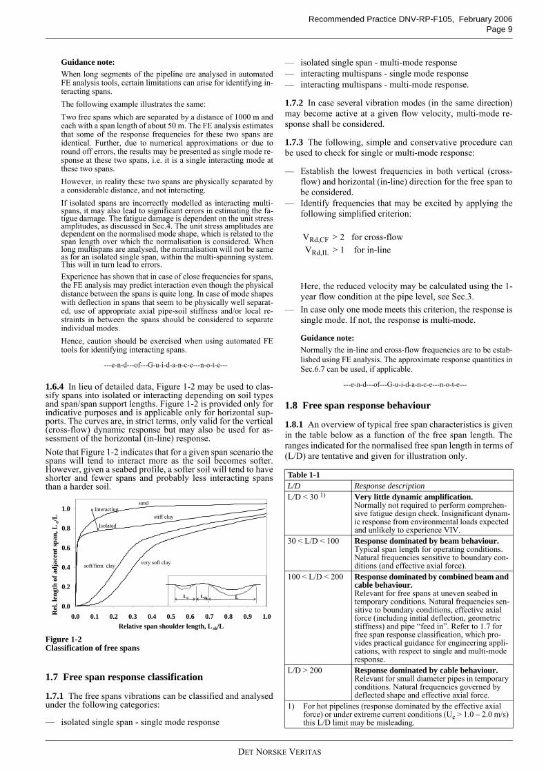
1.6.4 In lieu of detailed data, Figure 1-2 may be used to clas-sify spans into isolated or interacting depending on soil typesand span/span support lengths. Figure 1-2 is provided only forindicative purposes and is applicable only for horizontal sup-ports. The curves are, in strict terms, only valid for the vertical(cross-flow) dynamic response but may also be used for as-sessment of the horizontal (in-line) response.Note that Figure 1-2 indicates that for a given span scenario thespans will tend to interact more as the soil becomes softer.However, given a seabed profile, a softer soil will tend to haveshorter and fewer spans and probably less interacting spansthan a harder soil.
Figure 1-2Classification of free spans
1.7 Free span response classification
1.7.1 The free spans vibrations can be classified and analysedunder the following categories:
— isolated single span - single mode response
— isolated single span - multi-mode response— interacting multispans - single mode response— interacting multispans - multi-mode response.
1.7.2 In case several vibration modes (in the same direction)may become active at a given flow velocity, multi-mode re-sponse shall be considered.
1.7.3 The following, simple and conservative procedure canbe used to check for single or multi-mode response:
— Establish the lowest frequencies in both vertical (cross-flow) and horizontal (in-line) direction for the free span tobe considered.
— Identify frequencies that may be excited by applying thefollowing simplified criterion: VRd,CF > 2 for cross-flow VRd,IL > 1 for in-line
Here, the reduced velocity may be calculated using the 1-year flow condition at the pipe level, see Sec.3.
— In case only one mode meets this criterion, the response issingle mode. If not, the response is multi-mode.
Guidance note:Normally the in-line and cross-flow frequencies are to be estab-lished using FE analysis. The approximate response quantities inSec.6.7 can be used, if applicable.
---e-n-d---of---G-u-i-d-a-n-c-e---n-o-t-e---
1.8 Free span response behaviour
1.8.1 An overview of typical free span characteristics is givenin the table below as a function of the free span length. Theranges indicated for the normalised free span length in terms of(L/D) are tentative and given for illustration only.
0.0
0.2
0.4
0.6
0.8
1.0
0.0 0.1 0.2 0.3 0.4 0.5 0.6 0.7 0.8 0.9 1.0Relative span shoulder length, Lsh/L
Rel
. len
gth
of a
djac
ent s
pan,
La/L
La Lsh L
Isolated
Interacting
very soft claysoft/firm clay
stiff clay
sand
Table 1-1 L/D Response descriptionL/D < 30 1) Very little dynamic amplification.
Normally not required to perform comprehen-sive fatigue design check. Insignificant dynam-ic response from environmental loads expected and unlikely to experience VIV.
30 < L/D < 100 Response dominated by beam behaviour.Typical span length for operating conditions.Natural frequencies sensitive to boundary con-ditions (and effective axial force).
100 < L/D < 200 Response dominated by combined beam and cable behaviour. Relevant for free spans at uneven seabed in temporary conditions. Natural frequencies sen-sitive to boundary conditions, effective axial force (including initial deflection, geometric stiffness) and pipe “feed in”. Refer to 1.7 for free span response classification, which pro-vides practical guidance for engineering appli-cations, with respect to single and multi-mode response.
L/D > 200 Response dominated by cable behaviour.Relevant for small diameter pipes in temporary conditions. Natural frequencies governed by deflected shape and effective axial force.
1) For hot pipelines (response dominated by the effective axial force) or under extreme current conditions (Uc > 1.0 − 2.0 m/s) this L/D limit may be misleading.
DET NORSKE VERITAS
Recommended Practice DNV-RP-F105, February 2006 Page 10
1.9 Flow regimes
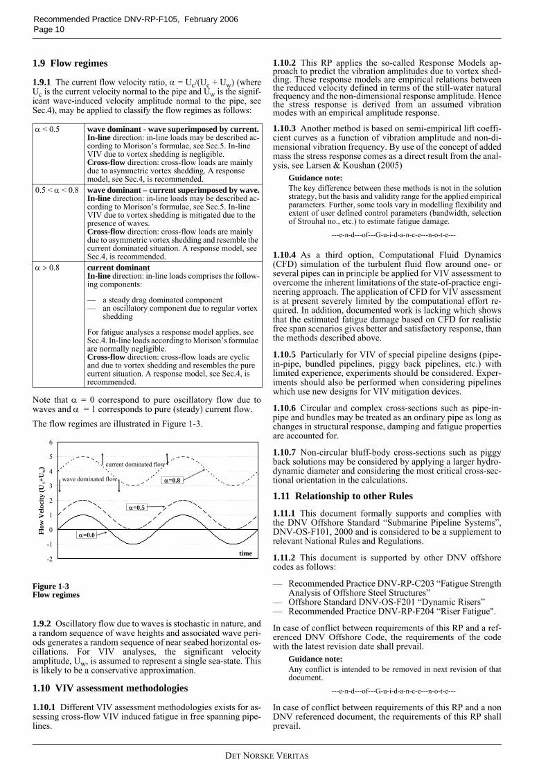
1.9.1 The current flow velocity ratio, α = Uc/(Uc + Uw) (whereUc is the current velocity normal to the pipe and Uw is the signif-icant wave-induced velocity amplitude normal to the pipe, seeSec.4), may be applied to classify the flow regimes as follows:
Note that α = 0 correspond to pure oscillatory flow due towaves and α = 1 corresponds to pure (steady) current flow.The flow regimes are illustrated in Figure 1-3.
Figure 1-3Flow regimes
1.9.2 Oscillatory flow due to waves is stochastic in nature, anda random sequence of wave heights and associated wave peri-ods generates a random sequence of near seabed horizontal os-cillations. For VIV analyses, the significant velocityamplitude, Uw, is assumed to represent a single sea-state. Thisis likely to be a conservative approximation.
1.10 VIV assessment methodologies
1.10.1 Different VIV assessment methodologies exists for as-sessing cross-flow VIV induced fatigue in free spanning pipe-lines.
1.10.2 This RP applies the so-called Response Models ap-proach to predict the vibration amplitudes due to vortex shed-ding. These response models are empirical relations betweenthe reduced velocity defined in terms of the still-water naturalfrequency and the non-dimensional response amplitude. Hencethe stress response is derived from an assumed vibrationmodes with an empirical amplitude response.
1.10.3 Another method is based on semi-empirical lift coeffi-cient curves as a function of vibration amplitude and non-di-mensional vibration frequency. By use of the concept of addedmass the stress response comes as a direct result from the anal-ysis, see Larsen & Koushan (2005)
Guidance note:The key difference between these methods is not in the solutionstrategy, but the basis and validity range for the applied empiricalparameters. Further, some tools vary in modelling flexibility andextent of user defined control parameters (bandwidth, selectionof Strouhal no., etc.) to estimate fatigue damage.
---e-n-d---of---G-u-i-d-a-n-c-e---n-o-t-e---
1.10.4 As a third option, Computational Fluid Dynamics(CFD) simulation of the turbulent fluid flow around one- orseveral pipes can in principle be applied for VIV assessment toovercome the inherent limitations of the state-of-practice engi-neering approach. The application of CFD for VIV assessmentis at present severely limited by the computational effort re-quired. In addition, documented work is lacking which showsthat the estimated fatigue damage based on CFD for realisticfree span scenarios gives better and satisfactory response, thanthe methods described above.
1.10.5 Particularly for VIV of special pipeline designs (pipe-in-pipe, bundled pipelines, piggy back pipelines, etc.) withlimited experience, experiments should be considered. Exper-iments should also be performed when considering pipelineswhich use new designs for VIV mitigation devices.
1.10.6 Circular and complex cross-sections such as pipe-in-pipe and bundles may be treated as an ordinary pipe as long aschanges in structural response, damping and fatigue propertiesare accounted for.
1.10.7 Non-circular bluff-body cross-sections such as piggyback solutions may be considered by applying a larger hydro-dynamic diameter and considering the most critical cross-sec-tional orientation in the calculations.
1.11 Relationship to other Rules
1.11.1 This document formally supports and complies withthe DNV Offshore Standard “Submarine Pipeline Systems”,DNV-OS-F101, 2000 and is considered to be a supplement torelevant National Rules and Regulations.
1.11.2 This document is supported by other DNV offshorecodes as follows:
— Recommended Practice DNV-RP-C203 “Fatigue StrengthAnalysis of Offshore Steel Structures”
— Offshore Standard DNV-OS-F201 “Dynamic Risers”— Recommended Practice DNV-RP-F204 “Riser Fatigue".
In case of conflict between requirements of this RP and a ref-erenced DNV Offshore Code, the requirements of the codewith the latest revision date shall prevail.
Guidance note:Any conflict is intended to be removed in next revision of thatdocument.
---e-n-d---of---G-u-i-d-a-n-c-e---n-o-t-e---
In case of conflict between requirements of this RP and a nonDNV referenced document, the requirements of this RP shallprevail.
α < 0.5 wave dominant - wave superimposed by current.In-line direction: in-line loads may be described ac-cording to Morison’s formulae, see Sec.5. In-line VIV due to vortex shedding is negligible.Cross-flow direction: cross-flow loads are mainly due to asymmetric vortex shedding. A response model, see Sec.4, is recommended.
0.5 < α < 0.8 wave dominant – current superimposed by wave.In-line direction: in-line loads may be described ac-cording to Morison’s formulae, see Sec.5. In-line VIV due to vortex shedding is mitigated due to the presence of waves.Cross-flow direction: cross-flow loads are mainly due to asymmetric vortex shedding and resemble the current dominated situation. A response model, see Sec.4, is recommended.
α > 0.8 current dominantIn-line direction: in-line loads comprises the follow-ing components:
— a steady drag dominated component— an oscillatory component due to regular vortex
shedding
For fatigue analyses a response model applies, see Sec.4. In-line loads according to Morison’s formulae are normally negligible.Cross-flow direction: cross-flow loads are cyclic and due to vortex shedding and resembles the pure current situation. A response model, see Sec.4, is recommended.
-2
-1
0
1
2
3
4
5
6
time
Flow
Vel
ocity
(Uc+
Uw) current dominated flow
wave dominated flow α=0.8
α=0.0
α=0.5
DET NORSKE VERITAS
Recommended Practice DNV-RP-F105, February 2006Page 11
1.12 Definitions
1.12.1 Effective Span Length is the length of an idealisedfixed-fixed span having the same structural response in termsof natural frequencies as the real free span supported on soil.
1.12.2 Force Model is in this document a model where the en-vironmental load is based on Morison’s force expression.
1.12.3 Gap is defined as the distance between the pipe and theseabed. The gap used in design, as a single representative val-ue, must be characteristic for the free spanThe gap may be calculated as the average value over the cen-tral third of the span.
1.12.4 Marginal Fatigue Capacity is defined as the fatigue ca-pacity (life) with respect to one sea state defined by its signif-icant wave height, peak period and direction.
1.12.5 Multi-mode Response, denotes response for a spanwhere several vibration modes may be excited simultaneouslyin the same direction (in-line or cross-flow).
1.12.6 Multi-spans are spans where the adjacent spans have ainfluence on the behaviour and response of a span.
1.12.7 Non-stationary Span is a span where the main spancharacteristics such as span length and gap change significant-ly over the design life, e.g. due to scouring of the seabed.
1.12.8 Response Model is a model where the structural re-sponse due to VIV is determined by hydrodynamic parameters.
1.12.9 Span Length is defined as the length where a continu-ous gap exists, i.e. as the visual span length.
1.12.10 Single Span is a span which is an isolated span thatcan be assessed independent of the neighbouring spans.
1.12.11 Stationary Span is a span where the main span charac-teristics such as span length and gap remain the same over thedesign life.
1.13 Abbreviations
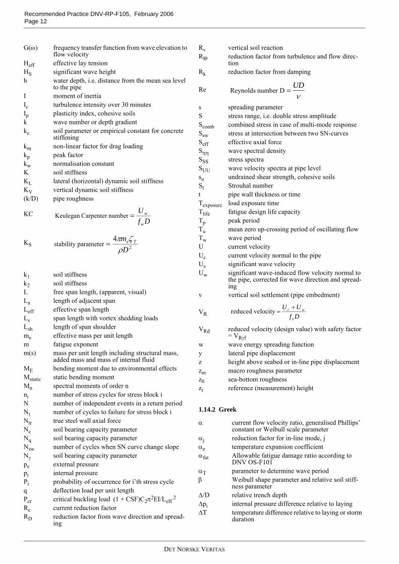
1.14 Symbols
1.14.1 Latin
CF cross-flowCSF concrete stiffness factorFLS fatigue limit stateFM force modelIL in-lineLRFD load and resistance factors design formatOCR over-consolidation ratio (only clays)RM response model (VIV)RD response domainRPV return period valuesSRSS square root of the sum of squaresTD time domainULS ultimate limit stateVIV vortex induced vibrations
aκ parameter for rain-flow counting factorcharacteristic fatigue strength constant
Ae external cross-section areaAi internal cross-section (bore) area
a
AIL in-line unit amplitude stress (stress induced by a pipe (vibration mode) deflection equal to an outer diameter D)
ACF cross-flow unit amplitude stress Ap cross sectional area of penetrated pipeAs pipe steel cross section area(AY/D) normalised in-line VIV amplitude(AZ/D) normalised cross-flow VIV amplitudeb linearisation constantB pipe-soil contact width bκ parameter for rain flow counting factorCa added mass coefficient (CM-1)Ca, CF-RES added mass coefficient due to cross-flow responseCD drag coefficientCD
0 basic drag coefficientCM the inertia coefficientCM
0 basic inertia coefficientCL coefficient for lateral soil stiffnessCV coefficient for vertical soil stiffnessCT constant for long-term wave period distributionC1-6 Boundary condition coefficientsc(s) soil damping per unit lengthd trench depthD pipe outer diameter (including any coating)Dfat deterministic fatigue damageDs outer steel diameterE Young's modulusEI bending stiffnesse seabed gapes void ratio(e/D) seabed gap ratiofcyc frequency used for fatigue stress cycle counting in
case of multimode responsefc frequency used for fatigue stress cycle counting in
case of multimode responsefn n’th eigen frequency of span in-line (fn,IL) or cross-
flow (fn,CF) natural frequency (determined at no flow around the pipe)
fcn concrete construction strengthfs vortex shedding frequency
F correction factor for pipe roughnessFL lateral pipe-soil contact forceFV vertical pipe-soil contact forcefv dominating vibration frequencyfw wave frequencyF() distribution functionFX cumulative distribution functiong acceleration of gravitygc correction function due to steady currentgD drag force termgI inertia force termG shear modulus of soil or incomplete complementa-
ry Gamma function
DUSt= frequency) (Strouhal
DET NORSKE VERITAS
Recommended Practice DNV-RP-F105, February 2006 Page 12
1.14.2 Greek
G(ω) frequency transfer function from wave elevation to flow velocity
Heff effective lay tensionHS significant wave heighth water depth, i.e. distance from the mean sea level
to the pipeI moment of inertiaIc turbulence intensity over 30 minutesIp plasticity index, cohesive soilsk wave number or depth gradientkc soil parameter or empirical constant for concrete
stiffeningkm non-linear factor for drag loadingkp peak factorkw normalisation constantK soil stiffnessKL lateral (horizontal) dynamic soil stiffnessKV vertical dynamic soil stiffness(k/D) pipe roughness
KC
KS
k1 soil stiffness k2 soil stiffnessL free span length, (apparent, visual)La length of adjacent spanLeff effective span lengthLs span length with vortex shedding loadsLsh length of span shoulderme effective mass per unit lengthm fatigue exponentm(s) mass per unit length including structural mass,
added mass and mass of internal fluidME bending moment due to environmental effectsMstatic static bending moment Mn spectral moments of order nni number of stress cycles for stress block iN number of independent events in a return periodNi number of cycles to failure for stress block iNtr true steel wall axial forceNc soil bearing capacity parameterNq soil bearing capacity parameterNsw number of cycles when SN curve change slopeNγ soil bearing capacity parameterpe external pressurepi internal pressure Pi probability of occurrence for i’th stress cycleq deflection load per unit lengthPcr critical buckling load (1 + CSF)C2π2EI/Leff
2
Rc current reduction factorRD reduction factor from wave direction and spread-
ing
DfU
w
w= numberCarpenter Keulegan
2
4parameterstability
Dm Te
ρζπ
=
Rv vertical soil reactionRIθ reduction factor from turbulence and flow direc-
tionRk reduction factor from damping
Re
s spreading parameterS stress range, i.e. double stress amplitudeScomb combined stress in case of multi-mode responseSsw stress at intersection between two SN-curvesSeff effective axial forceSηη wave spectral densitySSS stress spectraSUU wave velocity spectra at pipe levelsu undrained shear strength, cohesive soilsSt Strouhal numbert pipe wall thickness or timeTexposure load exposure timeTlife fatigue design life capacityTp peak periodTu mean zero up-crossing period of oscillating flowTw wave periodU current velocity Uc current velocity normal to the pipeUs significant wave velocityUw significant wave-induced flow velocity normal to
the pipe, corrected for wave direction and spread-ing
v vertical soil settlement (pipe embedment)
VR
VRd reduced velocity (design value) with safety factor = VRγf
w wave energy spreading functiony lateral pipe displacementz height above seabed or in-line pipe displacementzm macro roughness parameterz0 sea-bottom roughnesszr reference (measurement) height
α current flow velocity ratio, generalised Phillips’ constant or Weibull scale parameter
αj reduction factor for in-line mode, jαe temperature expansion coefficientαfat Allowable fatigue damage ratio according to
DNV OS-F101αT parameter to determine wave periodβ Weibull shape parameter and relative soil stiff-
ness parameter∆/D relative trench depth∆pi internal pressure difference relative to laying∆T temperature difference relative to laying or storm
duration
νUD =Dnumber Reynolds
DfUU
n
wc += velocityreduced
DET NORSKE VERITAS
Recommended Practice DNV-RP-F105, February 2006Page 13
1.14.3 Subscripts
2. Design Criteria2.1 General
2.1.1 For all temporary and permanent free spans a free spanassessment addressing the integrity with respect to fatigue(FLS) and local buckling (ULS) shall be performed.
2.1.2 Vibrations due to vortex shedding and direct wave loadsare acceptable provided the fatigue and ULS criteria specifiedherein are fulfilled.
2.1.3 In case several potential vibration modes can become activeat a given flow velocity, all these modes shall be considered. Un-less otherwise documented the damage contribution for everymode should relate to the same critical (weld) location.
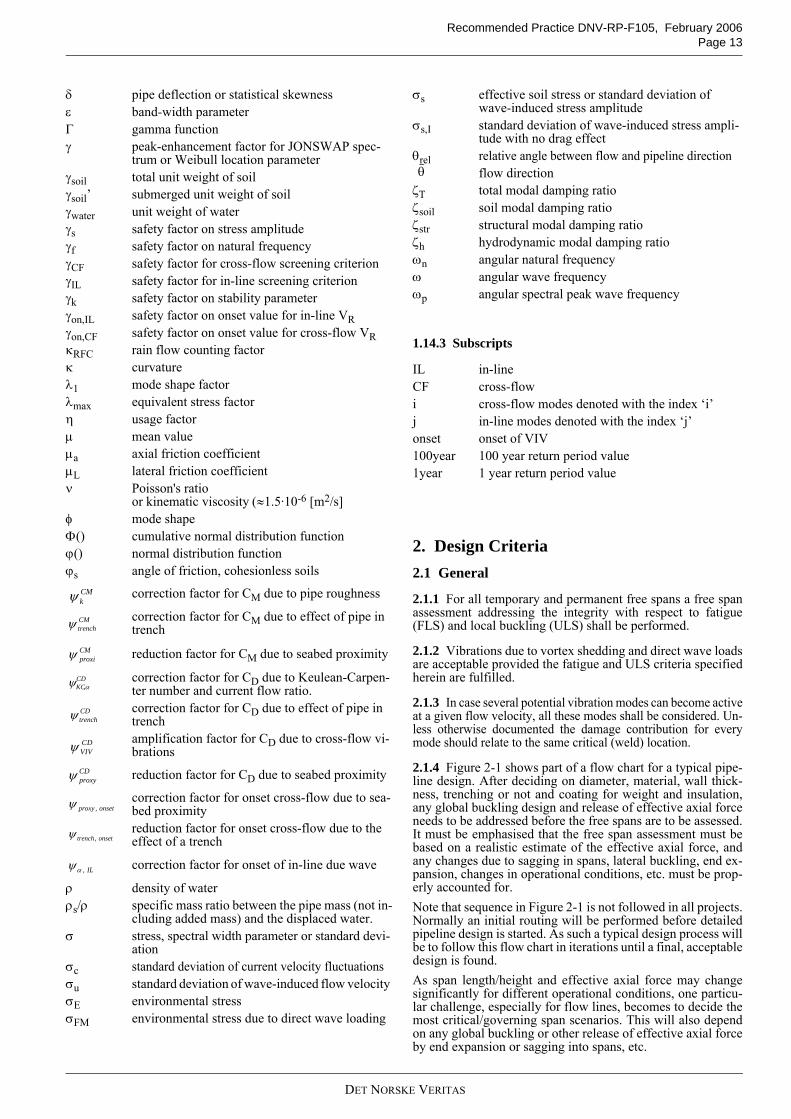
2.1.4 Figure 2-1 shows part of a flow chart for a typical pipe-line design. After deciding on diameter, material, wall thick-ness, trenching or not and coating for weight and insulation,any global buckling design and release of effective axial forceneeds to be addressed before the free spans are to be assessed.It must be emphasised that the free span assessment must bebased on a realistic estimate of the effective axial force, andany changes due to sagging in spans, lateral buckling, end ex-pansion, changes in operational conditions, etc. must be prop-erly accounted for.Note that sequence in Figure 2-1 is not followed in all projects.Normally an initial routing will be performed before detailedpipeline design is started. As such a typical design process willbe to follow this flow chart in iterations until a final, acceptabledesign is found.As span length/height and effective axial force may changesignificantly for different operational conditions, one particu-lar challenge, especially for flow lines, becomes to decide themost critical/governing span scenarios. This will also dependon any global buckling or other release of effective axial forceby end expansion or sagging into spans, etc.
δ pipe deflection or statistical skewnessε band-width parameterΓ gamma functionγ peak-enhancement factor for JONSWAP spec-
trum or Weibull location parameterγsoil total unit weight of soilγsoil’ submerged unit weight of soilγwater unit weight of waterγs safety factor on stress amplitudeγf safety factor on natural frequencyγCF safety factor for cross-flow screening criterionγIL safety factor for in-line screening criterionγk safety factor on stability parameterγon,IL safety factor on onset value for in-line VRγon,CF safety factor on onset value for cross-flow VRκRFC rain flow counting factorκ curvatureλ1 mode shape factorλmax equivalent stress factorη usage factorµ mean valueµa axial friction coefficientµL lateral friction coefficientν Poisson's ratio
or kinematic viscosity (≈1.5·10-6 [m2/s]φ mode shapeΦ() cumulative normal distribution functionϕ() normal distribution functionϕs angle of friction, cohesionless soils
correction factor for CM due to pipe roughness
correction factor for CM due to effect of pipe in trench
reduction factor for CM due to seabed proximity
correction factor for CD due to Keulean-Carpen-ter number and current flow ratio. correction factor for CD due to effect of pipe in trenchamplification factor for CD due to cross-flow vi-brations
reduction factor for CD due to seabed proximity
correction factor for onset cross-flow due to sea-bed proximityreduction factor for onset cross-flow due to the effect of a trench
correction factor for onset of in-line due wave
ρ density of waterρs/ρ specific mass ratio between the pipe mass (not in-
cluding added mass) and the displaced water.σ stress, spectral width parameter or standard devi-
ationσc standard deviation of current velocity fluctuationsσu standard deviation of wave-induced flow velocity σE environmental stressσFM environmental stress due to direct wave loading
CMkψCMtrenchψ
CMproxiψ
CD,KCαψ
CDtrenchψ
CDVIVψ
CDproxyψ
onset,proxyψ
onset,trenchψ
IL,αψ
σs effective soil stress or standard deviation of wave-induced stress amplitude
σs,I standard deviation of wave-induced stress ampli-tude with no drag effect
θrel relative angle between flow and pipeline directionflow direction
ζΤ total modal damping ratioζsoil soil modal damping ratioζstr structural modal damping ratioζh hydrodynamic modal damping ratioωn angular natural frequencyω angular wave frequencyωp angular spectral peak wave frequency
IL in-lineCF cross-flow i cross-flow modes denoted with the index ‘i’j in-line modes denoted with the index ‘j’onset onset of VIV100year 100 year return period value1year 1 year return period value
θ
DET NORSKE VERITAS
Recommended Practice DNV-RP-F105, February 2006 Page 14
Figure 2-1 Flow chart for pipeline design and free span design
2.1.5 The following functional requirements apply:
— The aim of fatigue design is to ensure an adequate safetyagainst fatigue failure within the design life of the pipe-line.
— The fatigue analysis should cover a period which is repre-sentative for the free span exposure period.
— All stress fluctuations imposed during the entire designlife of the pipeline capable of causing fatigue damage shallbe accounted for.
— The local fatigue design checks are to be performed at allfree spanning pipe sections accounting for damage contri-butions from all potential vibration modes related to theconsidered spans.
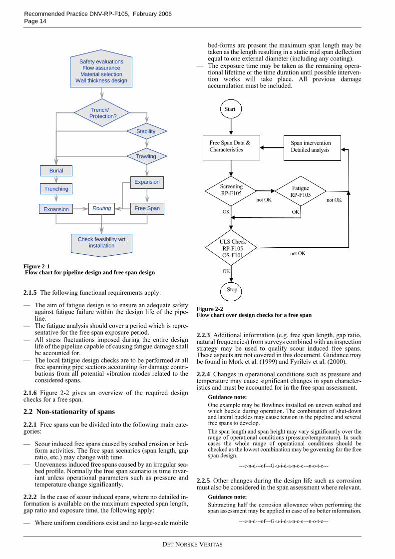
2.1.6 Figure 2-2 gives an overview of the required designchecks for a free span.
2.2 Non-stationarity of spans
2.2.1 Free spans can be divided into the following main cate-gories:
— Scour induced free spans caused by seabed erosion or bed-form activities. The free span scenarios (span length, gapratio, etc.) may change with time.
— Unevenness induced free spans caused by an irregular sea-bed profile. Normally the free span scenario is time invar-iant unless operational parameters such as pressure andtemperature change significantly.
2.2.2 In the case of scour induced spans, where no detailed in-formation is available on the maximum expected span length,gap ratio and exposure time, the following apply:
— Where uniform conditions exist and no large-scale mobile
bed-forms are present the maximum span length may betaken as the length resulting in a static mid span deflectionequal to one external diameter (including any coating).
— The exposure time may be taken as the remaining opera-tional lifetime or the time duration until possible interven-tion works will take place. All previous damageaccumulation must be included.
Figure 2-2Flow chart over design checks for a free span
2.2.3 Additional information (e.g. free span length, gap ratio,natural frequencies) from surveys combined with an inspectionstrategy may be used to qualify scour induced free spans.These aspects are not covered in this document. Guidance maybe found in Mørk et al. (1999) and Fyrileiv et al. (2000).
2.2.4 Changes in operational conditions such as pressure andtemperature may cause significant changes in span character-istics and must be accounted for in the free span assessment.
Guidance note:One example may be flowlines installed on uneven seabed andwhich buckle during operation. The combination of shut-downand lateral buckles may cause tension in the pipeline and severalfree spans to develop.The span length and span height may vary significantly over therange of operational conditions (pressure/temperature). In suchcases the whole range of operational conditions should bechecked as the lowest combination may be governing for the freespan design.
---e-n-d---of---G-u-i-d-a-n-c-e---n-o-t-e---
2.2.5 Other changes during the design life such as corrosionmust also be considered in the span assessment where relevant.
Guidance note:Subtracting half the corrosion allowance when performing thespan assessment may be applied in case of no better information.
---e-n-d---of---G-u-i-d-a-n-c-e---n-o-t-e---
Trenching Expansion
Expansion
Check feasibility wrt installation
Routing
Burial
Free Span
Trench/ Protection?
Safety evaluations Flow assurance
Material selection Wall thickness design
Trawling
Stability
Start
Free Span Data & Characteristics
OK
Screening RP-F105
Fatigue RP-F105
ULS Check RP-F105 OS-F101
Stop
Span intervention Detailed analysis
not OK
not OK
OK
OK
not OK
DET NORSKE VERITAS
Recommended Practice DNV-RP-F105, February 2006Page 15
2.3 Screening fatigue criteria
2.3.1 The screening criteria proposed herein apply to fatiguecaused by Vortex Induced Vibrations (VIV) and direct waveloading in combined current and wave loading conditions. Thescreening criteria have been calibrated against full fatigueanalyses to provide a fatigue life in excess of 50 years. The cri-teria apply to spans with a response dominated by the 1st sym-metric mode (one half wave) and should preferably be appliedfor screening analyses only. If violated, more detailed fatigueanalyses should be performed. The ULS criterion in 2.5 mustalways be checked.
Guidance note:The screening criteria as given in 2.3 are calibrated with safetyfactors to provide a fatigue life in excess of 50 years. As suchthese criteria are intended to be used for the operational phase.However, by applying the 10 year return period value for currentfor the appropriate season, Uc,10year, instead of the 100 year re-turn period value, the criteria may be used also for the temporaryphases (as-laid/empty and flooded).
---e-n-d---of---G-u-i-d-a-n-c-e---n-o-t-e---
2.3.2 The screening criteria proposed herein are based on theassumption that the current velocity may be represented by a3-parameter Weibull distribution. If this is not the case, e.g. forbi-modal current distributions, care must be taken and the ap-plicability of these screening criteria checked by full fatiguecalculations.
2.3.3 The in-line natural frequencies fn,IL must fulfil:
where
If the above criterion is violated, then a full in-line VIV fatigueanalysis is required.
2.3.4 The cross-flow natural frequencies fn,CF must fulfil:
where
If the above criterion is violated, then a full in-line and cross-flow VIV fatigue analysis is required.
2.3.5 If a fatigue analysis is required, a simplified estimate ofthe fatigue damage can be computed by adding the wave in-duced flow to the current long-term distribution or neglectingthe influence of the waves for deepwater pipelines. If this cri-terion is violated, then a full fatigue analyses due direct waveaction is required.
2.3.6 Fatigue analysis due to direct wave action is not requiredprovided:
and the above screening criteria for in-line VIV are fulfilled.If this criterion is violated, then a full fatigue analyses due toin-line VIV and direct wave action is required.
Guidance note:Section 2.3.6 states that full fatigue analysis is required if the 1-year significant wave-induced flow at pipe level is larger thanhalf the 100-year current velocity at pipe level. It is also possible to apply the screening criteria in the same wayas the traditional on-set criterion in order to establish conserva-tive allowable free span lengths even though the above men-tioned wave effect criterion is violated.If the flow is current dominated, the free span may be assessedby adding a characteristic wave-induced flow component to thecurrent velocity as expressed in the in-line VIV screening crite-rion, i.e. 1-year return period wave induced flow. If the flow velocity is dominated by the waves, then generally afull fatigue analysis has to be performed. However, the in-lineVIV screening criterion may still be used provided that a quasi-static Morison force calculation shows that the fatigue due to di-rect wave action could be neglected or is insignificant comparedto in-line VIV fatigue.
---e-n-d---of---G-u-i-d-a-n-c-e---n-o-t-e---
2.4 Fatigue criterion
2.4.1 The fatigue criterion can be formulated as:η ⋅ Tlife ≥ Texposure
where η is the allowable fatigue damage ratio, Tlife the fatiguedesign life capacity and Texposure the design life or load expo-sure time.
2.4.2 The fatigue damage assessment is based on the accumu-lation law by Palmgren-Miner:
where
2.4.3 The number of cycles to failure at stress range S is de-fined by the SN curve of the form:
where
γIL Screening factor for in-line, see 2.6
Minimum value of 0.6.D Outer pipe diameter incl. coatingL Free span lengthUc,100year 100 year return period value for the current velocity
at the pipe level, see Sec.3Uw,1year Significant 1 year return period value for the wave-
induced flow velocity at the pipe level correspond-ing to the annual significant wave height Hs,1year, see Sec.3In-line onset value for the reduced velocity, see Sec.4.
γCF Screening factor for cross-flow, see 2.6Cross-flow onset value for the reduced velocity, see Sec.4
αγ1
250/1
,
100,, ⋅⎟⎠⎞
⎜⎝⎛ −⋅
⋅>
DLDV
UfIL
onsetR
yearc
IL
ILn
αyear,cyear,w
year,c
UUU
1001
100 ratio flowCurrent +
=
ILonset,RV
DV
UUfCF
onsetR
yearwyearc
CF
CFn
⋅
+>
,
1,100,,
γ
CFonset,RV
Dfat Accumulated fatigue damage.ni Total number of stress cycles corresponding to the
(mid-wall) stress range SiN Number of cycles to failure at stress range SiΣ Implies summation over all stress fluctuations in the
design life
m1, m2 Fatigue exponents (the inverse slope of the bi-linear S-N curve)
32
UUU
year100,cyear1,w
year100,c >+
∑=i
ifat N
nD
⎪⎩
⎪⎨⎧
≤⋅>⋅
= −
−
swm
swm
SSSaSSSaN
22
11
DET NORSKE VERITAS
Recommended Practice DNV-RP-F105, February 2006 Page 16
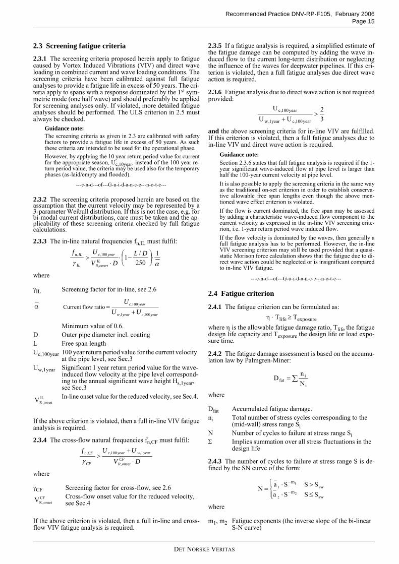
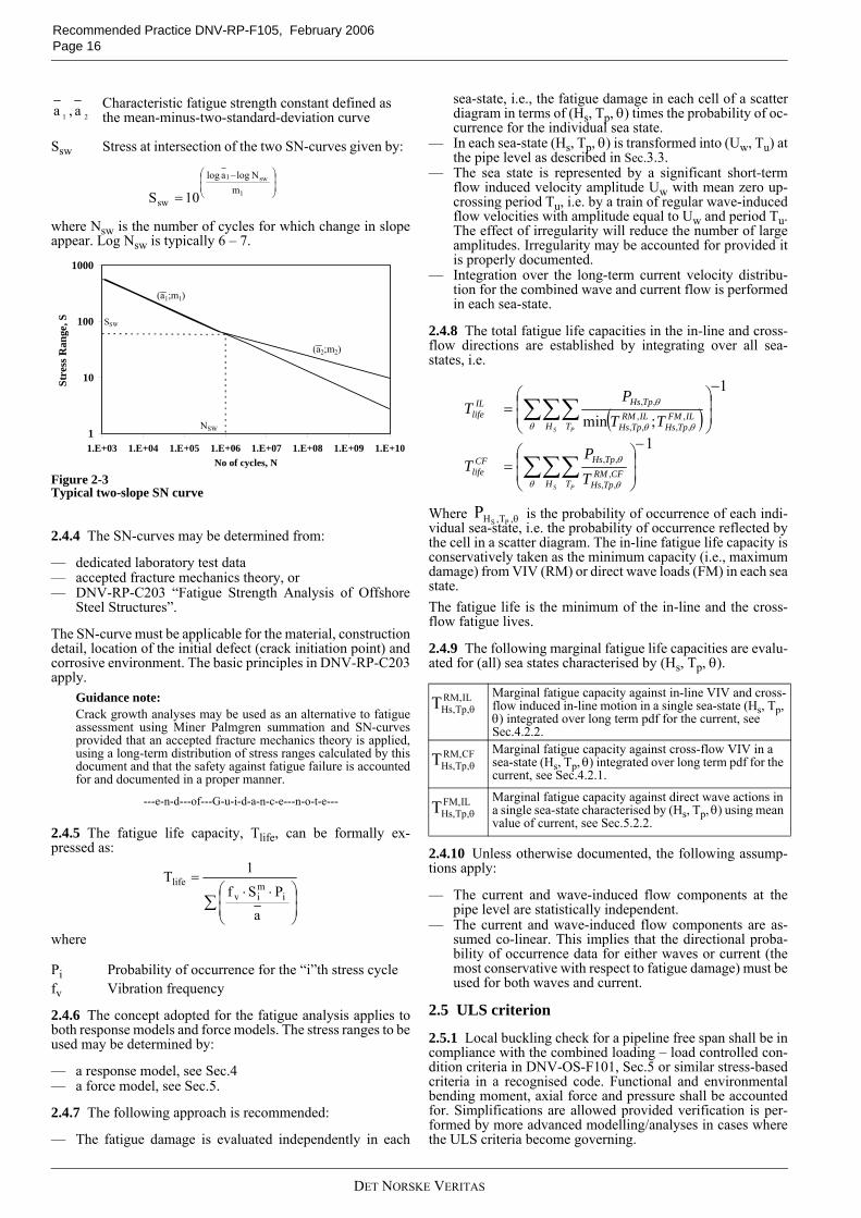
where Nsw is the number of cycles for which change in slopeappear. Log Nsw is typically 6 – 7.
Figure 2-3Typical two-slope SN curve
2.4.4 The SN-curves may be determined from:
— dedicated laboratory test data— accepted fracture mechanics theory, or— DNV-RP-C203 “Fatigue Strength Analysis of Offshore
Steel Structures”.
The SN-curve must be applicable for the material, constructiondetail, location of the initial defect (crack initiation point) andcorrosive environment. The basic principles in DNV-RP-C203apply.
Guidance note:Crack growth analyses may be used as an alternative to fatigueassessment using Miner Palmgren summation and SN-curvesprovided that an accepted fracture mechanics theory is applied,using a long-term distribution of stress ranges calculated by thisdocument and that the safety against fatigue failure is accountedfor and documented in a proper manner.
---e-n-d---of---G-u-i-d-a-n-c-e---n-o-t-e---
2.4.5 The fatigue life capacity, Tlife, can be formally ex-pressed as:
where
2.4.6 The concept adopted for the fatigue analysis applies toboth response models and force models. The stress ranges to beused may be determined by:
— a response model, see Sec.4— a force model, see Sec.5.
2.4.7 The following approach is recommended:
— The fatigue damage is evaluated independently in each
sea-state, i.e., the fatigue damage in each cell of a scatterdiagram in terms of (Hs, Tp, θ) times the probability of oc-currence for the individual sea state.
— In each sea-state (Hs, Tp, θ) is transformed into (Uw, Tu) atthe pipe level as described in Sec.3.3.
— The sea state is represented by a significant short-termflow induced velocity amplitude Uw with mean zero up-crossing period Tu, i.e. by a train of regular wave-inducedflow velocities with amplitude equal to Uw and period Tu.The effect of irregularity will reduce the number of largeamplitudes. Irregularity may be accounted for provided itis properly documented.
— Integration over the long-term current velocity distribu-tion for the combined wave and current flow is performedin each sea-state.
2.4.8 The total fatigue life capacities in the in-line and cross-flow directions are established by integrating over all sea-states, i.e.
Where is the probability of occurrence of each indi-vidual sea-state, i.e. the probability of occurrence reflected bythe cell in a scatter diagram. The in-line fatigue life capacity isconservatively taken as the minimum capacity (i.e., maximumdamage) from VIV (RM) or direct wave loads (FM) in each seastate.The fatigue life is the minimum of the in-line and the cross-flow fatigue lives.
2.4.9 The following marginal fatigue life capacities are evalu-ated for (all) sea states characterised by (Hs, Tp, θ).
2.4.10 Unless otherwise documented, the following assump-tions apply:
— The current and wave-induced flow components at thepipe level are statistically independent.
— The current and wave-induced flow components are as-sumed co-linear. This implies that the directional proba-bility of occurrence data for either waves or current (themost conservative with respect to fatigue damage) must beused for both waves and current.
2.5 ULS criterion
2.5.1 Local buckling check for a pipeline free span shall be incompliance with the combined loading – load controlled con-dition criteria in DNV-OS-F101, Sec.5 or similar stress-basedcriteria in a recognised code. Functional and environmentalbending moment, axial force and pressure shall be accountedfor. Simplifications are allowed provided verification is per-formed by more advanced modelling/analyses in cases wherethe ULS criteria become governing.
Characteristic fatigue strength constant defined as the mean-minus-two-standard-deviation curve
Ssw Stress at intersection of the two SN-curves given by:
Pi Probability of occurrence for the “i”th stress cyclefv Vibration frequency
21 a,a
⎟⎟⎠
⎞⎜⎜⎝
⎛ −
= 1
sw1
mNlogalog
sw 10S
1
10
100
1000
1.E+03 1.E+04 1.E+05 1.E+06 1.E+07 1.E+08 1.E+09 1.E+10No of cycles, N
Stre
ss R
ange
, S
NSW
SSW
(a1;m1)
(a2;m2)
∑ ⎟⎟⎠
⎞⎜⎜⎝
⎛ ⋅⋅=
aPSf
1Ti
miv
life
Marginal fatigue capacity against in-line VIV and cross-flow induced in-line motion in a single sea-state (Hs, Tp, θ) integrated over long term pdf for the current, see Sec.4.2.2.Marginal fatigue capacity against cross-flow VIV in a sea-state (Hs, Tp, θ) integrated over long term pdf for the current, see Sec.4.2.1.
Marginal fatigue capacity against direct wave actions in a single sea-state characterised by (Hs, Tp, θ) using mean value of current, see Sec.5.2.2.
( )1
1
;min
,,,
,,
,,,
,,,
,,
−
⎟⎟⎠
⎞⎜⎜⎝
⎛=
−
⎟⎟⎠
⎞⎜⎜⎝
⎛=
∑∑∑
∑∑∑
θ θ
θ
θ θθ
θ
S P
S P
H TCFRM
TpHs
TpHsCFlife
H TILFM
TpHsILRM
TpHs
TpHsILlife
TP
T
TTP
T
θ,T,H PSP
IL,RM,Tp,HsT θ
CF,RM,Tp,HsT θ
IL,FM,Tp,HsT θ
DET NORSKE VERITAS
Recommended Practice DNV-RP-F105, February 2006Page 17
2.5.2 Typically the load effects to be considered in the ULSchecks shall be:Vertical direction:
— static bending (self weight, seabed profile, etc.)— cross-flow VIV— trawl gear interaction.
Horizontal direction:
— in-line VIV— direct drag and inertia load effects from combined wave
and current— trawl gear interaction.
Note that different soil stiffnesses should be used for differentload directions and load rates (static/dynamic).
2.5.3 For the operating condition the environmental bendingmoment shall be taken as the most probable 100-year returnperiod value (10-2 annual exceedence probability). For tempo-rary conditions the return period value depends on the seasonaltiming and duration of the temporary period.
2.5.4 If more information is not available the following returnperiod values may be applied:
— A 100 year return period if the duration exceeds 6 months.— A 10 year return period for the actual seasonal environ-
mental condition if the duration exceeds 3 days but is lessthan 6 months.
— For temporary conditions with duration less than 3 days oroperations which can be terminated within a 3 days win-dow, environmental data may be based on reliable weatherforecasts.
2.5.5 Environmental events with a given return period requireinformation on joint wave and on-bottom current (and direc-tionality) probabilities. If more detailed information is notavailable the following cases may be applied (assuming co-lin-ear wave and current flow).
2.5.6 For extreme wave conditions, which can be assumed tocause large deformations on the span shoulders, detailed anal-yses of the soil stiffness at the shoulders may be required. Inlieu of detailed documentation, the boundary conditions for thefree span should be assumed as pinned-pinned (for direct waveload cases).
2.5.7 The maximum environmental bending moment due toin-line and cross-flow VIV or direct wave and current actionmay be found from the dynamic stresses:
where
2.5.8 The maximum environmental stress, σE, is taken as:
where
For the cross-flow direction, the stress simply stems from theVIV induced amplitude. For the in-line direction, the dynamicstress range is taken as the maximum of:
— the return period stress range for in-line VIV, SIL, definedin 4.3
— the stress from 40% of the CF induced VIV motion. Allparameters are defined in Sec.4.4.
2.5.9 Two different methods can be applied to establish themaximum environmental stress, σFM,max (see DNV-OS-F201for more information):
— design based on response statistics— design based on environmental statistics.
For free span analysis design based on environmental statisticsis considered appropriate using:
— a Design Storm approach with irregular wave analysis intime domain (TD) or irregular wave analyses in frequencydomain (FD), or
— a Design Wave approach using regular wave analysis inTD, i.e., with bending moment calculated from Hmax.
2.5.10 The Design Wave approach may use a set of appropri-ate design cases (in terms of wave height, wave period, currentand directionality) likely to produce the extreme response witha chosen return period. This may be done using a return periodvalue for Hs with a wave period variation covering a realisticvariation range (e.g. 90% confidence interval) or using envi-ronmental contours.
Guidance note:Cases with moderate Hs and large wave period are often govern-ing. Hence more focus should be given to large Tp values. In case of a quasi-static and not dynamically sensitive pipelineresponse for the ULS condition, the 100-year Hmax value with anassociated period could be used to generate the regular wave andcorresponding quasi-static response.
---e-n-d---of---G-u-i-d-a-n-c-e---n-o-t-e---
2.5.11 The maximum environmental stress, σFM,max, from di-rect wave loading can be established using a time domain De-sign Storm approach as follows:
1) Global time domain response analysis is performed for theactual stationary environmental condition. A typical stormduration may be taken as 3 hours.
2) Time histories for the dynamic stress are established 3) A 3-parameter Weibull distribution is fitted to the individ-
ual stress maxima between successive mean value cross-ings σFM(t).
(Hs, Tp) UcCase 1: 100 year 1 yearCase 2: 1 year 100 year
σE Maximum environmental stress given belowI Moment of inertiaDs Outer diameter of steel pipeT Wall thickness
tDIM
sEE −
⋅=
2σ
SIL In-line stress range, see Sec.4.3SCF Cross-flow stress range, see Sec.4.4σFM,max Maximum environmental stress due to direct wave
loading, see belowAIL In-line unit deflection stress amplitude due to VIV,
see Sec.4.3ACF Cross-flow unit deflection stress amplitude due to
VIV, see Sec.4.4
CFE
FMCF
ILCFILE
Sflowcross
AA
SSlinein
21
4.0;max21
max,
=−
+⎭⎬⎫
⎩⎨⎧
⋅=−
σ
σσ
DET NORSKE VERITAS
Recommended Practice DNV-RP-F105, February 2006 Page 18
4) A Gumbel distribution is established for the extreme valuefor the largest individual maxima of σFM(t) for the 3 hourduration.
5) σFM,max is estimated as the p-percentile in the Gumbel dis-tribution, i.e., the 57% percentile for the expected value orthe Most Probable Maximum value corresponding to a37% percentile
2.5.12 As a simplified alternative σFM,max may be calculatedusing:
where kp is a peak factor where ∆T is the storm duration equalto 3 hour and fv is the vibration frequency. σs is the standarddeviation of the stress response σFM(t) and σs,I is the standarddeviation for the stress response without drag loading. σs andσs,I may be calculated from a time domain or frequency do-main analysis, see Sec.5. kM is a factor accounting for non-lin-earity in the drag loading. A static stress component may beadded if relevant.
Guidance note:In case the ULS due to direct wave action is found to be govern-ing, the effect of the axial force should be considered.
---e-n-d---of---G-u-i-d-a-n-c-e---n-o-t-e---
2.5.13 For temporary conditions extreme environmental con-ditions, like a 10-year flow velocity sustained for a given timeperiod, may cause fatigue damage to develop. To ensure the in-tegrity of the pipeline and the robustness of the design, suchextreme events should be checked.
2.6 Safety factors
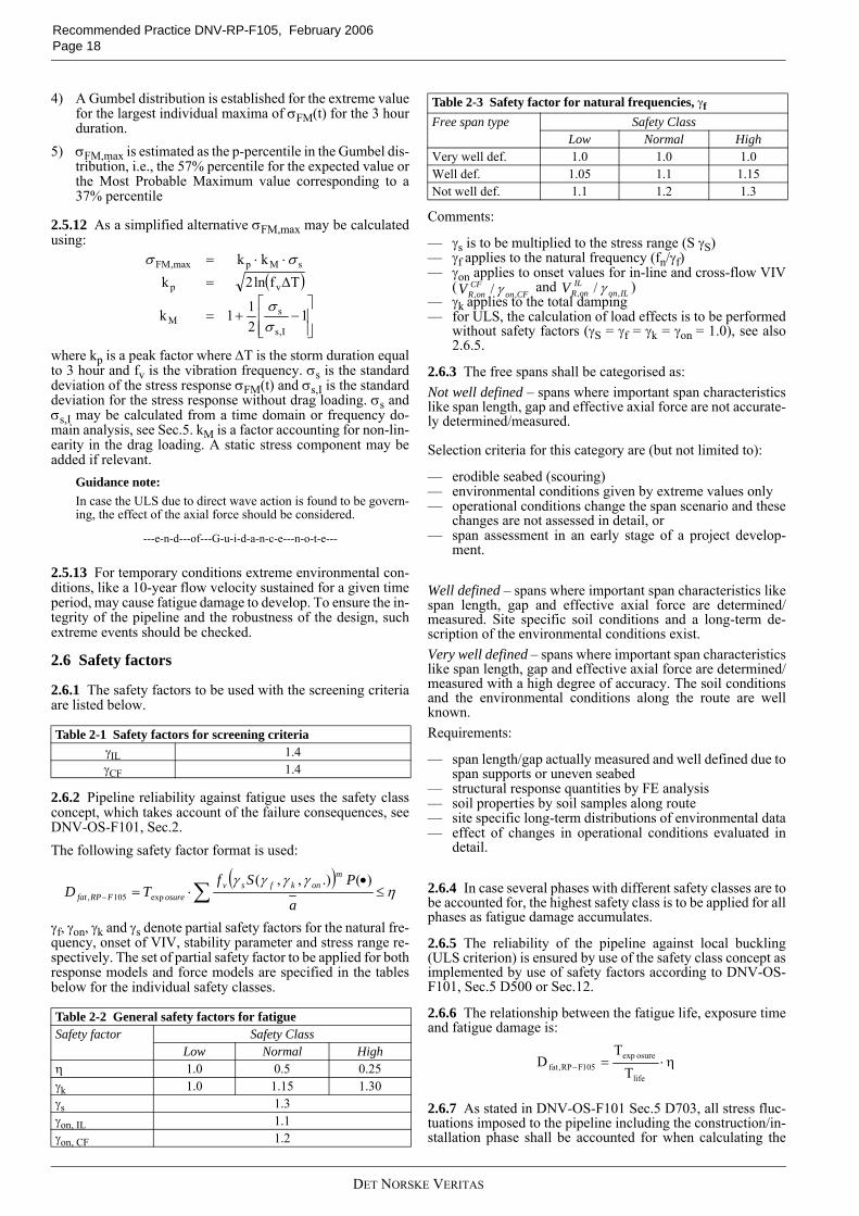
2.6.1 The safety factors to be used with the screening criteriaare listed below.
2.6.2 Pipeline reliability against fatigue uses the safety classconcept, which takes account of the failure consequences, seeDNV-OS-F101, Sec.2.The following safety factor format is used:
γf, γon, γk and γs denote partial safety factors for the natural fre-quency, onset of VIV, stability parameter and stress range re-spectively. The set of partial safety factor to be applied for bothresponse models and force models are specified in the tablesbelow for the individual safety classes.
Comments:
— γs is to be multiplied to the stress range (S γS)— γf applies to the natural frequency (fn/γf)— γon applies to onset values for in-line and cross-flow VIV
( and )— γk applies to the total damping— for ULS, the calculation of load effects is to be performed
without safety factors (γS = γf = γk = γon = 1.0), see also2.6.5.
2.6.3 The free spans shall be categorised as: Not well defined – spans where important span characteristicslike span length, gap and effective axial force are not accurate-ly determined/measured.
Selection criteria for this category are (but not limited to):
— erodible seabed (scouring)— environmental conditions given by extreme values only— operational conditions change the span scenario and these
changes are not assessed in detail, or— span assessment in an early stage of a project develop-
ment.
Well defined – spans where important span characteristics likespan length, gap and effective axial force are determined/measured. Site specific soil conditions and a long-term de-scription of the environmental conditions exist.Very well defined – spans where important span characteristicslike span length, gap and effective axial force are determined/measured with a high degree of accuracy. The soil conditionsand the environmental conditions along the route are wellknown.Requirements:
— span length/gap actually measured and well defined due tospan supports or uneven seabed
— structural response quantities by FE analysis— soil properties by soil samples along route— site specific long-term distributions of environmental data— effect of changes in operational conditions evaluated in
detail.
2.6.4 In case several phases with different safety classes are tobe accounted for, the highest safety class is to be applied for allphases as fatigue damage accumulates.
2.6.5 The reliability of the pipeline against local buckling(ULS criterion) is ensured by use of the safety class concept asimplemented by use of safety factors according to DNV-OS-F101, Sec.5 D500 or Sec.12.
2.6.6 The relationship between the fatigue life, exposure timeand fatigue damage is:
2.6.7 As stated in DNV-OS-F101 Sec.5 D703, all stress fluc-tuations imposed to the pipeline including the construction/in-stallation phase shall be accounted for when calculating the
Table 2-1 Safety factors for screening criteriaγIL 1.4γCF 1.4
Table 2-2 General safety factors for fatigueSafety factor Safety Class
Low Normal Highη 1.0 0.5 0.25γk 1.0 1.15 1.30γs 1.3
γon, IL 1.1γon, CF 1.2
( )
⎥⎥⎦
⎤
⎢⎢⎣
⎡−+=
∆=
⋅⋅=
1211k
Tfln2kkk
I,s
sM
vp
sMpmax,FM
σσ
σσ
( )η
γγγγ≤
•⋅= ∑−
a
PSfTD
monkfsv
osureFRPfat
)(.),,(exp105,
Table 2-3 Safety factor for natural frequencies, γfFree span type Safety Class
Low Normal HighVery well def. 1.0 1.0 1.0Well def. 1.05 1.1 1.15Not well def. 1.1 1.2 1.3
CFonCF
onRV ,, / γ ILonIL
onRV ,, / γ
η⋅=−
life
osureexp105FRP,fat T
TD
DET NORSKE VERITAS
Recommended Practice DNV-RP-F105, February 2006Page 19
fatigue damage. This means that the total accumulated fatiguedamage from different sources shall not exceed the allowabledamage ratios of DNV-OS-F101. As the allowable damage ra-tio of DNV-OS-F101 is different from the one in Table 2-2 dueto use of partial safety factors in RP-F105, the calculated dam-age ratio according to RP-F105 may be converted into a corre-sponding DNV-OS-F101 damage ratio by the followingrelation:
Where the αfat denotes the allowable damage ratio accordingto DNV-OS-F101.
3. Environmental Conditions3.1 General
3.1.1 The objective of the present section is to provide guid-ance on:
— the long term current velocity distribution— short-term and long-term description of wave-induced
flow velocity amplitude and period of oscillating flow atthe pipe level
— return period values.
3.1.2 The environmental data to be used in the assessment ofthe long-term distributions shall be representative for the par-ticular geographical location of the pipeline free span.
3.1.3 The flow conditions due to current and wave action atthe pipe level govern the response of free spanning pipelines.
3.1.4 The environmental data must be collected from periodsthat are representative for the long-term variation of the waveand current climate. In case of less reliable or limited wave andcurrent data, the statistical uncertainty should be assessed and,if significant, included in the analysis.
3.1.5 Preferably, the environmental load conditions should beestablished near the pipeline using measurement data of ac-ceptable quality and duration. The wave and current character-istics must be transferred (extrapolated) to the free span leveland location using appropriate conservative assumptions.
3.1.6 The following environmental description may be applied:
— directional information, i.e., flow characteristic versussector probability, or
— omnidirectional statistics may be used if the flow is uni-formly distributed.
If no such information is available, the flow should be assumedto act perpendicular to the axis of the pipeline at all times.
3.2 Current conditions
3.2.1 The steady current flow at the free span level may havecomponents from:
— tidal current— wind induced current— storm surge induced current— density driven current.
Guidance note:The effect of internal waves, which are often observed in parts ofSouth East Asia, need to be taken into account for the free spanassessment. The internal waves may have high fluid particle ve-locity and they can be modelled as equivalent current distribu-tions.
---e-n-d---of---G-u-i-d-a-n-c-e---n-o-t-e---
3.2.2 For water depths greater than 100 m, the ocean currentscan be characterised in terms of the driving and steeringagents:
— The driving agents are tidal forces, pressure gradients dueto surface elevation or density changes, wind and stormsurge forces.
— The steering agents are topography and the rotation of theearth.
The modelling should account adequately for all agents.
3.2.3 The flow can be divided into two zones:
— An Outer Zone far from the seabed where the mean cur-rent velocity and turbulence vary only slightly in the hori-zontal direction.
— An Inner Zone where the mean current velocity and tur-bulence show significant variations in the horizontal direc-tion and the current speed and direction is a function of thelocal sea bed geometry.
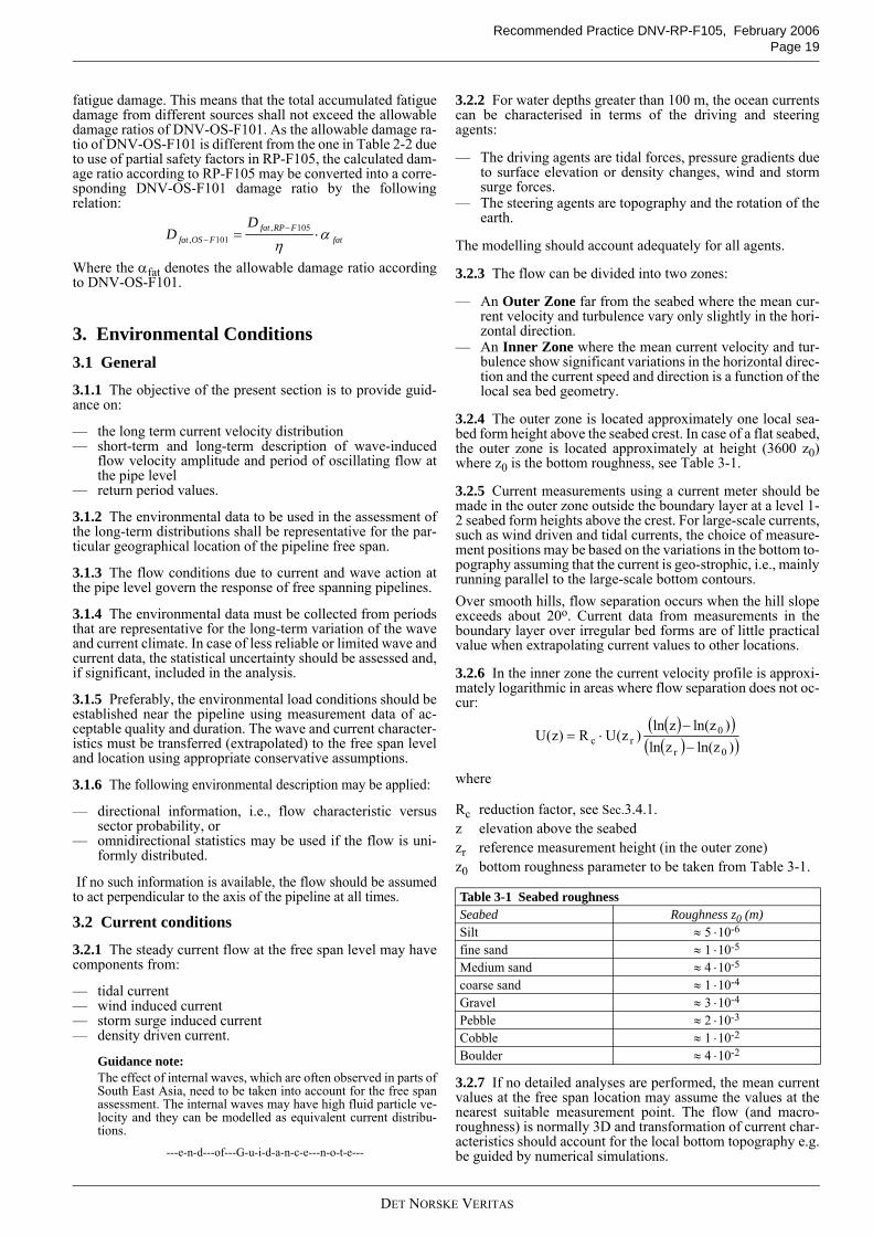
3.2.4 The outer zone is located approximately one local sea-bed form height above the seabed crest. In case of a flat seabed,the outer zone is located approximately at height (3600 z0)where z0 is the bottom roughness, see Table 3-1.
3.2.5 Current measurements using a current meter should bemade in the outer zone outside the boundary layer at a level 1-2 seabed form heights above the crest. For large-scale currents,such as wind driven and tidal currents, the choice of measure-ment positions may be based on the variations in the bottom to-pography assuming that the current is geo-strophic, i.e., mainlyrunning parallel to the large-scale bottom contours. Over smooth hills, flow separation occurs when the hill slopeexceeds about 20o. Current data from measurements in theboundary layer over irregular bed forms are of little practicalvalue when extrapolating current values to other locations.
3.2.6 In the inner zone the current velocity profile is approxi-mately logarithmic in areas where flow separation does not oc-cur:
where
3.2.7 If no detailed analyses are performed, the mean currentvalues at the free span location may assume the values at thenearest suitable measurement point. The flow (and macro-roughness) is normally 3D and transformation of current char-acteristics should account for the local bottom topography e.g.be guided by numerical simulations.
fatFRPfat
FOSfat
DD α
η⋅= −
−105,
101,
Rc reduction factor, see Sec.3.4.1.z elevation above the seabedzr reference measurement height (in the outer zone)z0 bottom roughness parameter to be taken from Table 3-1.
Table 3-1 Seabed roughnessSeabed Roughness z0 (m)Silt ≈ 5 ⋅10-6
fine sand ≈ 1 ⋅10-5
Medium sand ≈ 4 ⋅10-5
coarse sand ≈ 1 ⋅10-4
Gravel ≈ 3 ⋅10-4
Pebble ≈ 2 ⋅10-3
Cobble ≈ 1 ⋅10-2
Boulder ≈ 4 ⋅10-2
( )( )( )( ))zln(zln
)zln(zln)z(UR)z(U
0r
0rc −
−⋅=
DET NORSKE VERITAS
Recommended Practice DNV-RP-F105, February 2006 Page 20
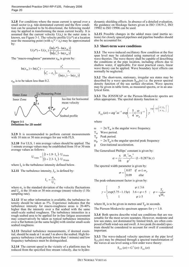
3.2.8 For conditions where the mean current is spread over asmall sector (e.g. tide-dominated current) and the flow condi-tion can be assumed to be bi-directional, the following modelmay be applied in transforming the mean current locally. It isassumed that the current velocity U(zr) in the outer zone isknown, see Figure 3-1. The velocity profile U(z*) at a locationnear the measuring point (with zr* > zr) may be approximatedby:
The “macro-roughness” parameter zm is given by:
zm is to be taken less than 0.2.
Figure 3-1Definitions for 2D model
3.2.9 It is recommended to perform current measurementswith 10 min or 30 min averages for use with FLS.
3.2.10 For ULS, 1 min average values should be applied. The1 minute average values may be established from 10 or 30 minaverage values as follows:
where Ic is the turbulence intensity defined below.
3.2.11 The turbulence intensity, Ic, is defined by:
where σc is the standard deviation of the velocity fluctuationsand Uc is the 10 min or 30 min average (mean) velocity (1 Hzsampling rate).
3.2.12 If no other information is available, the turbulence in-tensity should be taken as 5%. Experience indicates that theturbulence intensity for macro-roughness areas is 20-40%higher than the intensity over a flat seabed with the samesmall-scale seabed roughness. The turbulence intensities in arough seabed area to be applied for in-line fatigue assessmentmay conservatively be taken as typical turbulence intensitiesover a flat bottom (at the same height) with similar small-scaleseabed roughness.
3.2.13 Detailed turbulence measurements, if deemed essen-tial, should be made at 1 m and 3 m above the seabed. High fre-quency turbulence (with periods lower than 1 minute) and lowfrequency turbulence must be distinguished.
3.2.14 The current speed in the vicinity of a platform may bereduced from the specified free stream velocity, due to hydro-
dynamic shielding effects. In absence of a detailed evaluation,the guidance on blockage factors given in ISO 13819-2, ISO19902 to ISO 19906 can be used.
3.2.15 Possible changes in the added mass (and inertia ac-tions) for closely spaced pipelines and pipeline bundles shouldalso be accounted for.
3.3 Short-term wave conditions
3.3.1 The wave-induced oscillatory flow condition at the freespan level may be calculated using numerical or analyticalwave theories. The wave theory shall be capable of describingthe conditions at the pipe location, including effects due toshallow water, if applicable. For most practical cases, linearwave theory can be applied. Wave boundary layer effects cannormally be neglected.
3.3.2 The short-term, stationary, irregular sea states may bedescribed by a wave spectrum Sηη(ω) i.e. the power spectraldensity function of the sea surface elevation. Wave spectramay be given in table form, as measured spectra, or in an ana-lytical form.
3.3.3 The JONSWAP or the Pierson-Moskowitz spectra areoften appropriate. The spectral density function is:
where
The Generalised Phillips’ constant is given by:
The spectral width parameter is given by:
The peak-enhancement factor is given by:
where Hs is to be given in metres and Tp in seconds.The Pierson-Moskowitz spectrum appears for γ = 1.0.
3.3.4 Both spectra describe wind sea conditions that are rea-sonable for the most severe seastates. However, moderate andlow sea states, not dominated by limited fetch, are often com-posed of both wind-sea and swell. A two peak (bi-modal) spec-trum should be considered to account for swell if consideredimportant.
3.3.5 The wave-induced velocity spectrum at the pipe levelSUU(ω) may be obtained through a spectral transformation ofthe waves at sea level using a first order wave theory:
( )( )( )( ))zln(zln
)zln(*zln)z(U*)z(U
m*r
mr
−
−=
( ) ( ))zln()zln(z
zz
z)zln()zln(
or
rrr
rrm
−+−
−=∗
∗∗
z*z*r
zZr
Seabed profile
Iso-line for horisontalmean velocity
Outer ZoneInner Zone
U0 Measuring Point
( )( )⎩
⎨⎧
⋅⋅+⋅⋅+
=min30c
min10cmin1 UI3.21
UI9.11U
c
cc U
Iσ
=
ω = 2π/Tw is the angular wave frequency.Tw Wave period.Tp Peak period.ωp = 2π/Tp is the angular spectral peak frequencyg Gravitational acceleration.
⎟⎟⎟
⎠
⎞
⎜⎜⎜
⎝
⎛
⎟⎟
⎠
⎞
⎜⎜
⎝
⎛ −−
−−
⎟⎟⎠
⎞⎜⎜⎝
⎛−=
2
5.0exp452 )(
45exp)(
p
p
p
gSωσ
ωω
ηη γωωωαω
)ln287.01(165
2
42
γω
α −⋅⋅=g
H ps
⎩⎨⎧ ≤
=else
if p
09.007.0 ωω
σ
S
p
HT
=⎪⎩
⎪⎨
⎧
≥<<−
≤= ϕ
ϕϕϕ
ϕγ ;
5156.3)15.175.5exp(
6.35
)()()( 2 ωωω ηηSGSUU ⋅=
DET NORSKE VERITAS
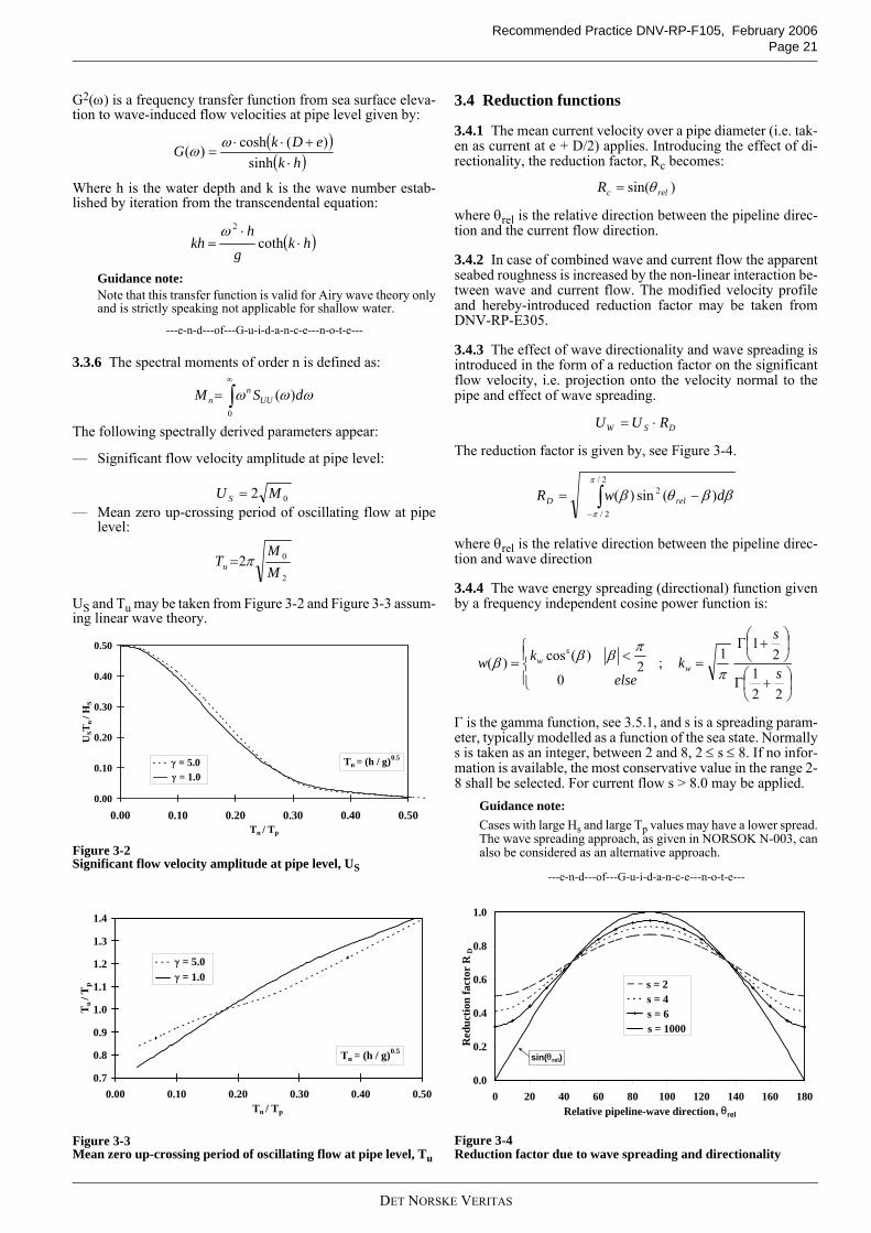
Recommended Practice DNV-RP-F105, February 2006Page 21
G2(ω) is a frequency transfer function from sea surface eleva-tion to wave-induced flow velocities at pipe level given by:
Where h is the water depth and k is the wave number estab-lished by iteration from the transcendental equation:
Guidance note:Note that this transfer function is valid for Airy wave theory onlyand is strictly speaking not applicable for shallow water.
---e-n-d---of---G-u-i-d-a-n-c-e---n-o-t-e---
3.3.6 The spectral moments of order n is defined as:
The following spectrally derived parameters appear:
— Significant flow velocity amplitude at pipe level:
— Mean zero up-crossing period of oscillating flow at pipelevel:
US and Tu may be taken from Figure 3-2 and Figure 3-3 assum-ing linear wave theory.
Figure 3-2Significant flow velocity amplitude at pipe level, US
Figure 3-3Mean zero up-crossing period of oscillating flow at pipe level, Tu
3.4 Reduction functions
3.4.1 The mean current velocity over a pipe diameter (i.e. tak-en as current at e + D/2) applies. Introducing the effect of di-rectionality, the reduction factor, Rc becomes:
where θrel is the relative direction between the pipeline direc-tion and the current flow direction.
3.4.2 In case of combined wave and current flow the apparentseabed roughness is increased by the non-linear interaction be-tween wave and current flow. The modified velocity profileand hereby-introduced reduction factor may be taken fromDNV-RP-E305.
3.4.3 The effect of wave directionality and wave spreading isintroduced in the form of a reduction factor on the significantflow velocity, i.e. projection onto the velocity normal to thepipe and effect of wave spreading.
The reduction factor is given by, see Figure 3-4.
where θrel is the relative direction between the pipeline direc-tion and wave direction
3.4.4 The wave energy spreading (directional) function givenby a frequency independent cosine power function is:
Γ is the gamma function, see 3.5.1, and s is a spreading param-eter, typically modelled as a function of the sea state. Normallys is taken as an integer, between 2 and 8, 2 ≤ s ≤ 8. If no infor-mation is available, the most conservative value in the range 2-8 shall be selected. For current flow s > 8.0 may be applied.
Guidance note:Cases with large Hs and large Tp values may have a lower spread.The wave spreading approach, as given in NORSOK N-003, canalso be considered as an alternative approach.
---e-n-d---of---G-u-i-d-a-n-c-e---n-o-t-e---
Figure 3-4Reduction factor due to wave spreading and directionality
( )( )hk
eDkG⋅
+⋅⋅=
sinh)(cosh)( ωω
( )hkg
hkh ⋅
⋅= coth
2ω
ωωω dSM UUn
n ∫∞
=0
)(
02 MU S =
2
02MM
Tu π=
0.00
0.10
0.20
0.30
0.40
0.50
0.00 0.10 0.20 0.30 0.40 0.50Tn / Tp
UST
n/ H
S
γ = 5.0γ = 1.0
Tn = (h / g)0.5
0.7
0.8
0.9
1.0
1.1
1.2
1.3
1.4
0.00 0.10 0.20 0.30 0.40 0.50Tn / Tp
Tu
/ Tp
γ = 5.0γ = 1.0
Tn = (h / g)0.5
)sin( relcR θ=
DSW RUU ⋅=
∫−
−=2/
2/
2 )(sin)(π
π
ββθβ dwR relD
⎟⎠⎞
⎜⎝⎛ +Γ
⎟⎠⎞
⎜⎝⎛ +Γ
=⎪⎩
⎪⎨⎧ <=
221
21
1;0
2)(cos)(
s
s
kelse
kw w
sw
π
πβββ
0.0
0.2
0.4
0.6
0.8
1.0
0 20 40 60 80 100 120 140 160 180Relative pipeline-wave direction, θrel
Red
uctio
n fa
ctor
RD
s = 2s = 4s = 6s = 1000
sin(θrel)
DET NORSKE VERITAS
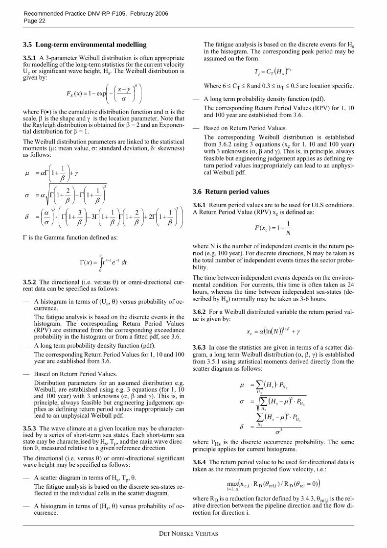
Recommended Practice DNV-RP-F105, February 2006 Page 22
3.5 Long-term environmental modelling
3.5.1 A 3-parameter Weibull distribution is often appropriatefor modelling of the long-term statistics for the current velocityUc or significant wave height, Hs. The Weibull distribution isgiven by:
where F(•) is the cumulative distribution function and α is thescale, β is the shape and γ is the location parameter. Note thatthe Rayleigh distribution is obtained for β = 2 and an Exponen-tial distribution for β = 1. The Weibull distribution parameters are linked to the statisticalmoments (µ: mean value, σ: standard deviation, δ: skewness)as follows:
Γ is the Gamma function defined as:
3.5.2 The directional (i.e. versus θ) or omni-directional cur-rent data can be specified as follows:
— A histogram in terms of (Uc, θ) versus probability of oc-currence.The fatigue analysis is based on the discrete events in thehistogram. The corresponding Return Period Values(RPV) are estimated from the corresponding exceedanceprobability in the histogram or from a fitted pdf, see 3.6.
— A long term probability density function (pdf).The corresponding Return Period Values for 1, 10 and 100year are established from 3.6.
— Based on Return Period Values.Distribution parameters for an assumed distribution e.g.Weibull, are established using e.g. 3 equations (for 1, 10and 100 year) with 3 unknowns (α, β and γ). This is, inprinciple, always feasible but engineering judgement ap-plies as defining return period values inappropriately canlead to an unphysical Weibull pdf.
3.5.3 The wave climate at a given location may be character-ised by a series of short-term sea states. Each short-term seastate may be characterised by Hs, Tp, and the main wave direc-tion θ, measured relative to a given reference directionThe directional (i.e. versus θ) or omni-directional significantwave height may be specified as follows:
— A scatter diagram in terms of Hs, Tp, θ.The fatigue analysis is based on the discrete sea-states re-flected in the individual cells in the scatter diagram.
— A histogram in terms of (Hs, θ) versus probability of oc-currence.
The fatigue analysis is based on the discrete events for Hsin the histogram. The corresponding peak period may beassumed on the form:
Where 6 ≤ CT ≤ 8 and 0.3 ≤ αT ≤ 0.5 are location specific.
— A long term probability density function (pdf).The corresponding Return Period Values (RPV) for 1, 10and 100 year are established from 3.6.
— Based on Return Period Values.The corresponding Weibull distribution is establishedfrom 3.6.2 using 3 equations (xc for 1, 10 and 100 year)with 3 unknowns (α, β and γ). This is, in principle, alwaysfeasible but engineering judgement applies as defining re-turn period values inappropriately can lead to an unphysi-cal Weibull pdf.
3.6 Return period values
3.6.1 Return period values are to be used for ULS conditions.A Return Period Value (RPV) xc is defined as:
where N is the number of independent events in the return pe-riod (e.g. 100 year). For discrete directions, N may be taken asthe total number of independent events times the sector proba-bility.The time between independent events depends on the environ-mental condition. For currents, this time is often taken as 24hours, whereas the time between independent sea-states (de-scribed by Hs) normally may be taken as 3-6 hours.
3.6.2 For a Weibull distributed variable the return period val-ue is given by:
3.6.3 In case the statistics are given in terms of a scatter dia-gram, a long term Weibull distribution (α, β, γ) is establishedfrom 3.5.1 using statistical moments derived directly from thescatter diagram as follows:
where PHs is the discrete occurrence probability. The sameprinciple applies for current histograms.
3.6.4 The return period value to be used for directional data istaken as the maximum projected flow velocity, i.e.:
where RD is a reduction factor defined by 3.4.3, θrel,i is the rel-ative direction between the pipeline direction and the flow di-rection for direction i.
⎟⎟⎠
⎞⎜⎜⎝
⎛⎟⎠⎞
⎜⎝⎛ −
−−=β
αγxxFX exp1)(
⎟⎟
⎠
⎞
⎜⎜
⎝
⎛⎟⎟⎠
⎞⎜⎜⎝
⎛+Γ+⎟⎟
⎠
⎞⎜⎜⎝
⎛+Γ⎟⎟
⎠
⎞⎜⎜⎝
⎛+Γ−⎟⎟
⎠
⎞⎜⎜⎝
⎛+Γ⋅⎟
⎠⎞
⎜⎝⎛=
⎟⎟⎠
⎞⎜⎜⎝
⎛+Γ−⎟⎟
⎠
⎞⎜⎜⎝
⎛+Γ=
+⎟⎟⎠
⎞⎜⎜⎝
⎛+Γ=
33
2
1122111331
1121
11
ββββσαδ
ββασ
γβ
αµ
∫∞
−−=Γ0
1)( dtetx tx
( ) TsTp HCT α=
NxF c
11)( −=
( )( ) γα β += /1ln Nxc
( )
( )
( )3
3
2
σ
µδ
µσ
µ
∑∑
∑
⋅−=
⋅−=
⋅=
S
S
S
S
S
S
HHs
HHs
HHs
PH
PH
PH
( ))0(R/)(Rxmax relDi,relDi,cn..1i
=⋅=
θθ
DET NORSKE VERITAS
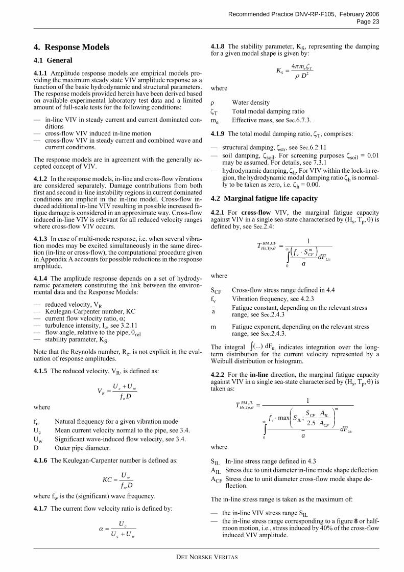
Recommended Practice DNV-RP-F105, February 2006Page 23
4. Response Models4.1 General
4.1.1 Amplitude response models are empirical models pro-viding the maximum steady state VIV amplitude response as afunction of the basic hydrodynamic and structural parameters.The response models provided herein have been derived basedon available experimental laboratory test data and a limitedamount of full-scale tests for the following conditions:
— in-line VIV in steady current and current dominated con-ditions
— cross-flow VIV induced in-line motion— cross-flow VIV in steady current and combined wave and
current conditions.
The response models are in agreement with the generally ac-cepted concept of VIV.
4.1.2 In the response models, in-line and cross-flow vibrationsare considered separately. Damage contributions from bothfirst and second in-line instability regions in current dominatedconditions are implicit in the in-line model. Cross-flow in-duced additional in-line VIV resulting in possible increased fa-tigue damage is considered in an approximate way. Cross-flowinduced in-line VIV is relevant for all reduced velocity rangeswhere cross-flow VIV occurs.
4.1.3 In case of multi-mode response, i.e. when several vibra-tion modes may be excited simultaneously in the same direc-tion (in-line or cross-flow), the computational procedure givenin Appendix A accounts for possible reductions in the responseamplitude.
4.1.4 The amplitude response depends on a set of hydrody-namic parameters constituting the link between the environ-mental data and the Response Models:
— reduced velocity, VR— Keulegan-Carpenter number, KC— current flow velocity ratio, α;— turbulence intensity, Ic, see 3.2.11— flow angle, relative to the pipe, θrel— stability parameter, KS.
Note that the Reynolds number, Re, is not explicit in the eval-uation of response amplitudes.
4.1.5 The reduced velocity, VR, is defined as:
where
4.1.6 The Keulegan-Carpenter number is defined as:
where fw is the (significant) wave frequency.
4.1.7 The current flow velocity ratio is defined by:
4.1.8 The stability parameter, KS, representing the dampingfor a given modal shape is given by:
where
4.1.9 The total modal damping ratio, ζT, comprises:
— structural damping, ζstr, see Sec.6.2.11— soil damping, ζsoil. For screening purposes ζsoil = 0.01
may be assumed. For details, see 7.3.1— hydrodynamic damping, ζh. For VIV within the lock-in re-
gion, the hydrodynamic modal damping ratio ζh is normal-ly to be taken as zero, i.e. ζh = 0.00.
4.2 Marginal fatigue life capacity
4.2.1 For cross-flow VIV, the marginal fatigue capacityagainst VIV in a single sea-state characterised by (Hs, Tp, θ) isdefined by, see Sec.2.4:
where
The integral indicates integration over the long-term distribution for the current velocity represented by aWeibull distribution or histogram.
4.2.2 For the in-line direction, the marginal fatigue capacityagainst VIV in a single sea-state characterised by (Hs, Tp, θ) istaken as:
where
The in-line stress range is taken as the maximum of:
— the in-line VIV stress range SIL — the in-line stress range corresponding to a figure 8 or half-
moon motion, i.e., stress induced by 40% of the cross-flowinduced VIV amplitude.
fn Natural frequency for a given vibration mode Uc Mean current velocity normal to the pipe, see 3.4.Uw Significant wave-induced flow velocity, see 3.4.D Outer pipe diameter.
DfUU
Vn
wcR
+=
DfU
KCw
w=
wc
c
UUU+
=α
ρ Water densityζT Total modal damping ratiome Effective mass, see Sec.6.7.3.
SCF Cross-flow stress range defined in 4.4 fv Vibration frequency, see 4.2.3
Fatigue constant, depending on the relevant stress range, see Sec.2.4.3
m Fatigue exponent, depending on the relevant stress range, see Sec.2.4.3.
SIL In-line stress range defined in 4.3AIL Stress due to unit diameter in-line mode shape deflectionACF Stress due to unit diameter cross-flow mode shape de-
flection.
24
DmK Te
S ρζπ
=
( )∫∞ ⋅
=
0
,,,
1
Uc
mCFv
CFRMTpHs
dFaSf
T θ
a
∫ cudF(...)
∫∞ ⎟
⎟⎠
⎞⎜⎜⎝
⎛⋅
=
0
,,,
5.2;max
1
Uc
m
CF
ILCFILv
ILRMTpHs
dFa
AAS
Sf
T θ
DET NORSKE VERITAS
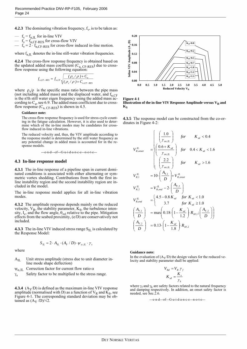
Recommended Practice DNV-RP-F105, February 2006 Page 24
4.2.3 The dominating vibration frequency, fv, is to be taken as:
— fv = fn,IL for in-line VIV— fv = fn,CF-RES for cross-flow VIV— fv = 2 ⋅ fn,CF-RES for cross-flow induced in-line motion.
where fn,IL denotes the in-line still-water vibration frequencies.
4.2.4 The cross-flow response frequency is obtained based onthe updated added mass coefficient (Ca, CF-RES) due to cross-flow response using the following equation:
where ρs/ρ is the specific mass ratio between the pipe mass(not including added mass) and the displaced water, and fn,CFis the n'th still water eigen frequency using the added mass ac-cording to Ca, see 6.9. The added mass coefficient due to cross-flow response (Ca, CF-RES) is shown in 4.5.
Guidance note:The cross-flow response frequency is used for stress cycle count-ing in the fatigue calculation. However, it is also used to deter-mine which of the in-line modes may be candidates for cross-flow induced in-line vibrations.The reduced velocity and, thus, the VIV amplitude according tothe response model is determined by the still water frequency asany potential change in added mass is accounted for in the re-sponse models.
---e-n-d---of---G-u-i-d-a-n-c-e---n-o-t-e---
4.3 In-line response model
4.3.1 The in-line response of a pipeline span in current domi-nated conditions is associated with either alternating or sym-metric vortex shedding. Contributions from both the first in-line instability region and the second instability region are in-cluded in the model. The in-line response model applies for all in-line vibrationmodes.
4.3.2 The amplitude response depends mainly on the reducedvelocity, VR, the stability parameter, KS, the turbulence inten-sity, Ic, and the flow angle, θrel relative to the pipe. Mitigationeffects from the seabed proximity, (e/D) are conservatively notincluded.
4.3.3 The in-line VIV induced stress range SIL is calculated bythe Response Model:
where
4.3.4 (AY/D) is defined as the maximum in-line VIV responseamplitude (normalised with D) as a function of VR and KS, seeFigure 4-1. The corresponding standard deviation may be ob-tained as (AY /D)/√2.
Figure 4-1Illustration of the in-line VIV Response Amplitude versus VR andKS
4.3.5 The response model can be constructed from the co-or-dinates in Figure 4-2:
Guidance note:In the evaluation of (AY/D) the design values for the reduced ve-locity and stability parameter shall be applied:
where γf and γk are safety factors related to the natural frequencyand damping respectively. In addition, an onset safety factor isneeded, see Sec.2.6.
---e-n-d---of---G-u-i-d-a-n-c-e---n-o-t-e---
AIL Unit stress amplitude (stress due to unit diameter in-line mode shape deflection)
ψα,IL Correction factor for current flow ratio αγs Safety factor to be multiplied to the stress range.
RESCF,as
asCF,nRESCF,n C)/(
C)/(ff−
− ++
=ρρ
ρρ
sILYILIL DAAS γψ α ⋅⋅⋅⋅= ,)/(2
0.00
0.04
0.08
0.12
0.16
0.20
0.0 0.5 1.0 1.5 2.0 2.5 3.0 3.5 4.0 4.5 5.0
Inlin
e V
IV A
mpl
itude
(Ay/D
)
Ksd=0.0
Reduced Velocity VR
Ksd=1.5
Ksd=1.2
Ksd=1.0
Ksd=0.7
Ksd=0.5
Ksd=0.2
2,2,
2,1,
1,
,
2,,2,
,1,
1,
,
,
,
,
8.1113.0
;2.1
118.0max
0.17.30.18.05.4
2
10
6.12.2
6.14.06.0
4.00.1
θ
θ
γ
γ
γ
IsdY
YI
sdY
sd
sdsdILendR
YILendR
ILR
ILonsetR
YILR
sdILon
sdILon
sd
sdILon
ILonsetR
RK
DA
DA
RK
DA
KforKforK
V
DA
VV
VD
AV
Kfor
KforK
Kfor
V
⋅⎟⎟⎠
⎞⎜⎜⎝
⎛−⋅=⎟⎟
⎠
⎞⎜⎜⎝
⎛
⎟⎟⎠
⎞⎜⎜⎝
⎛⎟⎟⎠
⎞⎜⎜⎝
⎛⋅⎟⎟
⎠
⎞⎜⎜⎝
⎛−⋅=⎟⎟
⎠
⎞⎜⎜⎝
⎛⎩⎨⎧
≥<−
=
⎟⎟⎠
⎞⎜⎜⎝
⎛⋅−=
+⎟⎟⎠
⎞⎜⎜⎝
⎛⋅=
⎪⎪⎪⎪
⎩
⎪⎪⎪⎪
⎨
⎧
>⎟⎟⎠
⎞⎜⎜⎝
⎛
<<⎟⎟⎠
⎞⎜⎜⎝
⎛ +
<⎟⎟⎠
⎞⎜⎜⎝
⎛
=
k
ssd
fRRd
KK
VV
γ
γ
=
=
DET NORSKE VERITAS
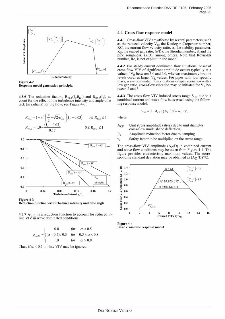
Recommended Practice DNV-RP-F105, February 2006Page 25
Figure 4-2Response model generation principle.
4.3.6 The reduction factors, RIθ,1(Ic,θrel) and RIθ,2(Ic), ac-count for the effect of the turbulence intensity and angle of at-tack (in radians) for the flow, see Figure 4-3.
Figure 4-3Reduction function wrt turbulence intensity and flow angle
4.3.7 ψα,IL is a reduction function to account for reduced in-line VIV in wave dominated conditions:
Thus, if α < 0.5, in-line VIV may be ignored.
4.4 Cross-flow response model
4.4.1 Cross-flow VIV are affected by several parameters, suchas the reduced velocity VR, the Keulegan-Carpenter number,KC, the current flow velocity ratio, α, the stability parameter,KS, the seabed gap ratio, (e/D), the Strouhal number, St and thepipe roughness, (k/D), among others. Note that Reynoldsnumber, Re, is not explicit in the model.
4.4.2 For steady current dominated flow situations, onset ofcross-flow VIV of significant amplitude occurs typically at avalue of VR between 3.0 and 4.0, whereas maximum vibrationlevels occur at larger VR values. For pipes with low specificmass, wave dominated flow situations or span scenarios with alow gap ratio, cross-flow vibration may be initiated for VR be-tween 2 and 3.
4.4.3 The cross-flow VIV induced stress range SCF due to acombined current and wave flow is assessed using the follow-ing response model:
where
The cross-flow VIV amplitude (AZ/D) in combined currentand wave flow conditions may be taken from Figure 4-4. Thefigure provides characteristic maximum values. The corre-sponding standard deviation may be obtained as (AZ /D)/√2.
Figure 4-4Basic cross-flow response model
Inlin
e V
IV A
mpl
itude
( )0;V ILend,R
⎟⎠⎞
⎜⎝⎛
DAY
Reduced Velocity
⎟⎟⎠
⎞⎜⎜⎝
⎛⎟⎟⎠
⎞⎜⎜⎝
⎛D
A;V 1,YIL
1,R
⎟⎟⎠
⎞⎜⎜⎝
⎛⎟⎟⎠
⎞⎜⎜⎝
⎛D
A;V 2,YIL
2,R
( )0;V ILonset,R
( )( )
1017.0
03.00.1
1003.022
1
2,2,
1,2
1,
≤≤−
−=
≤≤−⎟⎠⎞
⎜⎝⎛ ⋅−−=
θθ
θθ θππ
Ic
I
IcrelI
RI
R
RIR
1.0
0.8
0.6
0.4
0.2
0.00.04 0.12 0.16 0.2
Turbulence Intensity, Ic
0.080
Ri θ,1 θ = 60°
Ri θ,1 θ = 45°
Ri θ,1 θ = 30°
Ri θ,1 θ = 0°
Ri θ,2
all angles
⎪⎩
⎪⎨
⎧
><<−
<= 8.0
8.00.15.03.0/)5.0(
5.00.0
,
ααα
αψ α
forforfor
IL
ACF Unit stress amplitude (stress due to unit diameter cross-flow mode shape deflection)
Rk Amplitude reduction factor due to damping γs Safety factor to be multiplied on the stress range
skZCFCF RDAAS γ⋅⋅⋅⋅= )/(2
0.0
0.2
0.4
0.6
0.8
1.0
1.2
1.4
0 2 4 6 8 10 12 14 16
cronset,RV
Reduced Velocity VR
> 0.8 ;
< 0.8 ; KC < 10
< 0.8 ; KC > 30
3.2CF,nfCF,1nf
>⎟⎠⎞
⎜⎝⎛ +
5.1CF,nfCF,1nf
<⎟⎠⎞
⎜⎝⎛ +
α
α
α
Cro
ss-F
low
VIV
Am
plitu
de (A
Z/ D
)
DET NORSKE VERITAS
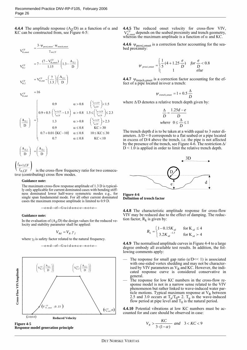
Recommended Practice DNV-RP-F105, February 2006 Page 26
4.4.4 The amplitude response (AZ/D) as a function of α andKC can be constructed from, see Figure 4-5:
is the cross-flow frequency ratio for two consecu-tive (contributing) cross flow modes.
Guidance note:The maximum cross-flow response amplitude of 1.3 D is typical-ly only applicable for current dominated cases with bending stiff-ness dominated lower half-wave symmetric modes e.g., forsingle span fundamental mode. For all other current dominatedcases the maximum response amplitude is limited to 0.9 D.
---e-n-d---of---G-u-i-d-a-n-c-e---n-o-t-e---
Guidance note:In the evaluation of (AZ/D) the design values for the reduced ve-locity and stability parameter shall be applied:
where γf is safety factor related to the natural frequency.
---e-n-d---of---G-u-i-d-a-n-c-e---n-o-t-e---
Figure 4-5Response model generation principle
4.4.5 The reduced onset velocity for cross-flow VIV,depends on the seabed proximity and trench geometry,
whereas the maximum amplitude is a function of α and KC.
4.4.6 ψproxi,onset is a correction factor accounting for the sea-bed proximity:
4.4.7 ψtrench,onset is a correction factor accounting for the ef-fect of a pipe located in/over a trench:
where ∆/D denotes a relative trench depth given by:
The trench depth d is to be taken at a width equal to 3 outer di-ameters. ∆/D = 0 corresponds to a flat seabed or a pipe locatedin excess of D/4 above the trench, i.e. the pipe is not affectedby the presence of the trench, see Figure 4-6. The restriction ∆/D < 1.0 is applied in order to limit the relative trench depth.
Figure 4-6Definition of trench factor
4.4.8 The characteristic amplitude response for cross-flowVIV may be reduced due to the effect of damping. The reduc-tion factor, Rk is given by:
4.4.9 The normalised amplitude curves in Figure 4-4 to a largedegree embody all available test results. In addition, the fol-lowing comments apply:
— The response for small gap ratio (e/D<< 1) is associatedwith one-sided vortex shedding and may not be character-ised by VIV parameters as VR and KC. However, the indi-cated response curve is considered conservative ingeneral.
— The response for low KC numbers in the cross-flow re-sponse model is not in a narrow sense related to the VIVphenomenon but rather linked to wave-induced water par-ticle motions. Typical maximum response at VR between2.5 and 3.0 occurs at Tu/T0≈ 2. Tu is the wave-inducedflow period at pipe level and T0 is the natural period.
4.4.10 Potential vibrations at low KC numbers must be ac-counted for and care should be observed in case:
( )
⎟⎟⎠
⎞⎜⎜⎝
⎛=⎟⎟
⎠
⎞⎜⎜⎝
⎛
⎪⎪⎪⎪⎪
⎩
⎪⎪⎪⎪⎪
⎨
⎧
<≤α≤≤≤α−⋅+
>≤α
>⎟⎠⎞
⎜⎝⎛>α
≤⎟⎠⎞
⎜⎝⎛≤>α⎟
⎠⎞
⎜⎝⎛ −⋅+
<⎟⎠⎞
⎜⎝⎛>α
=⎟⎟⎠
⎞⎜⎜⎝
⎛
=
⎟⎟⎠
⎞⎜⎜⎝
⎛⋅⎟
⎠⎞
⎜⎝⎛−=
⎟⎟⎠
⎞⎜⎜⎝
⎛−⋅
−−=
γ
ψ⋅ψ⋅=
+
++
+
DA
DA
10KC8.07.030KC108.010KC01.07.0
30KC8.09.0
3.28.03.1
3.25.18.05.15.09.0
5.18.09.0
DA
16V
DA
3.17V
V
DA
3.115.1
)V7(7
V
3V
1,Z2,Z
CF,nfCF,1nf
CF,nfCF,1nf
CF,nfCF,1nf
CF,nfCF,1nf
1,Z
CFend,R
1,ZCFend,RCF
2,R
1,ZCF
onset,RCF
1,R
CF,on
onset,trenchonset,proxiCF
onset,R
( )CF,nfCF,nf 1+
fRRd VV γ=
Cro
ss-F
low
VIV
Am
plitu
de
Reduced Velocity
⎟⎟⎠
⎞⎜⎜⎝
⎛⎟⎟⎠
⎞⎜⎜⎝
⎛D
A;V 2,ZCF
2,R⎟⎟⎠
⎞⎜⎜⎝
⎛⎟⎟⎠
⎞⎜⎜⎝
⎛D
A;V 1,ZCF
1,R
( )0;V CFend,R
( )0.0;0.2
( )15.0;V CFonset,R
CFonset,RV
⎪⎩
⎪⎨⎧ <+=
elseDefor
De
onsetproxi1
8.0)25.14(51
,ψ
Donsettrench∆
+= 5.01,ψ
10
25.1
≤∆
≤
−=
∆
Dwhere
Ded
D
d
D
e
3D
⎩⎨⎧ ≤−
= − 4Kfor 4Kfor
3.215.01
sd5.1
fsd
sd
sdk K
KR
93)1(3
<<−⋅
> KCandKCVR α
DET NORSKE VERITAS
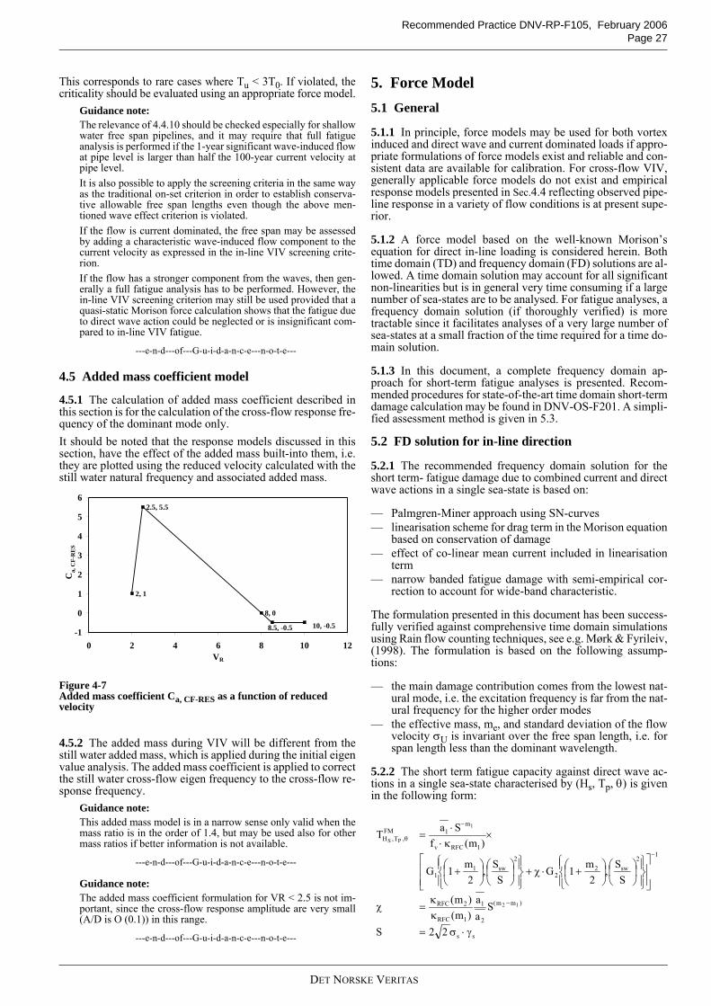
Recommended Practice DNV-RP-F105, February 2006Page 27
This corresponds to rare cases where Tu < 3T0. If violated, thecriticality should be evaluated using an appropriate force model.
Guidance note:The relevance of 4.4.10 should be checked especially for shallowwater free span pipelines, and it may require that full fatigueanalysis is performed if the 1-year significant wave-induced flowat pipe level is larger than half the 100-year current velocity atpipe level. It is also possible to apply the screening criteria in the same wayas the traditional on-set criterion in order to establish conserva-tive allowable free span lengths even though the above men-tioned wave effect criterion is violated.If the flow is current dominated, the free span may be assessedby adding a characteristic wave-induced flow component to thecurrent velocity as expressed in the in-line VIV screening crite-rion. If the flow has a stronger component from the waves, then gen-erally a full fatigue analysis has to be performed. However, thein-line VIV screening criterion may still be used provided that aquasi-static Morison force calculation shows that the fatigue dueto direct wave action could be neglected or is insignificant com-pared to in-line VIV fatigue.
---e-n-d---of---G-u-i-d-a-n-c-e---n-o-t-e---
4.5 Added mass coefficient model
4.5.1 The calculation of added mass coefficient described inthis section is for the calculation of the cross-flow response fre-quency of the dominant mode only. It should be noted that the response models discussed in thissection, have the effect of the added mass built-into them, i.e.they are plotted using the reduced velocity calculated with thestill water natural frequency and associated added mass.
Figure 4-7Added mass coefficient Ca, CF-RES as a function of reduced velocity
4.5.2 The added mass during VIV will be different from thestill water added mass, which is applied during the initial eigenvalue analysis. The added mass coefficient is applied to correctthe still water cross-flow eigen frequency to the cross-flow re-sponse frequency.
Guidance note:This added mass model is in a narrow sense only valid when themass ratio is in the order of 1.4, but may be used also for othermass ratios if better information is not available.
---e-n-d---of---G-u-i-d-a-n-c-e---n-o-t-e---
Guidance note:The added mass coefficient formulation for VR < 2.5 is not im-portant, since the cross-flow response amplitude are very small(A/D is O (0.1)) in this range.
---e-n-d---of---G-u-i-d-a-n-c-e---n-o-t-e---
5. Force Model5.1 General
5.1.1 In principle, force models may be used for both vortexinduced and direct wave and current dominated loads if appro-priate formulations of force models exist and reliable and con-sistent data are available for calibration. For cross-flow VIV,generally applicable force models do not exist and empiricalresponse models presented in Sec.4.4 reflecting observed pipe-line response in a variety of flow conditions is at present supe-rior.
5.1.2 A force model based on the well-known Morison’sequation for direct in-line loading is considered herein. Bothtime domain (TD) and frequency domain (FD) solutions are al-lowed. A time domain solution may account for all significantnon-linearities but is in general very time consuming if a largenumber of sea-states are to be analysed. For fatigue analyses, afrequency domain solution (if thoroughly verified) is moretractable since it facilitates analyses of a very large number ofsea-states at a small fraction of the time required for a time do-main solution.
5.1.3 In this document, a complete frequency domain ap-proach for short-term fatigue analyses is presented. Recom-mended procedures for state-of-the-art time domain short-termdamage calculation may be found in DNV-OS-F201. A simpli-fied assessment method is given in 5.3.
5.2 FD solution for in-line direction
5.2.1 The recommended frequency domain solution for theshort term- fatigue damage due to combined current and directwave actions in a single sea-state is based on:
— Palmgren-Miner approach using SN-curves— linearisation scheme for drag term in the Morison equation
based on conservation of damage— effect of co-linear mean current included in linearisation
term— narrow banded fatigue damage with semi-empirical cor-
rection to account for wide-band characteristic.
The formulation presented in this document has been success-fully verified against comprehensive time domain simulationsusing Rain flow counting techniques, see e.g. Mørk & Fyrileiv,(1998). The formulation is based on the following assump-tions:
— the main damage contribution comes from the lowest nat-ural mode, i.e. the excitation frequency is far from the nat-ural frequency for the higher order modes
— the effective mass, me, and standard deviation of the flowvelocity σU is invariant over the free span length, i.e. forspan length less than the dominant wavelength.
5.2.2 The short term fatigue capacity against direct wave ac-tions in a single sea-state characterised by (Hs, Tp, θ) is givenin the following form:
2, 1
2.5, 5.5
8, 0
10, -0.58.5, -0.5-1
0
1
2
3
4
5
6
0 2 4 6 8 10 12VR
Ca,
CF-
RE
S
ss
)mm(
2
1
1RFC
2RFC
12
sw22
2sw1
1
1RFCv
m1FM
,T,H
22S
Saa
)m()m(
SS,
2m1G
SS,
2m1G
)m(fSaT
12
1
PS
γ⋅σ=κκ
=χ
⎥⎥⎦
⎤
⎢⎢⎣
⎡
⎪⎭
⎪⎬⎫
⎪⎩
⎪⎨⎧
⎟⎠⎞
⎜⎝⎛
⎟⎠⎞
⎜⎝⎛ +⋅χ+
⎪⎭
⎪⎬⎫
⎪⎩
⎪⎨⎧
⎟⎠⎞
⎜⎝⎛
⎟⎠⎞
⎜⎝⎛ +
×κ⋅
⋅=
−
−
−
θ
DET NORSKE VERITAS
Recommended Practice DNV-RP-F105, February 2006 Page 28
where
5.2.3 The standard deviation of the wave-induced stress am-plitude σS is given by the square root of the spectral momentof the 0th order defined by 5.2.6.
5.2.4 The characteristic vibration frequency of consideredpipe stress response, fv, is taken equal to the mean up-crossingfrequency defined by:
M0 and M2 is defined by 5.2.6.
5.2.5 The rain flow counting correction factor, κRFC, accountsfor the “exact” wide-banded damage, i.e. correcting the implic-it narrow-banded Rayleigh assumption for the stress ampli-tudes to provide results similar to those arising from a state-of-the-art rain flow counting technique. The Rain Flow Countingfactor κRFC is given by:
The bandwidth parameter ε is defined as:
The stress process is narrow-banded for ε → 0 and broad band-ed for ε → 1 (in practice the process may be considered broad-banded for ε larger than 0.6).
5.2.6 The nth response spectral moment is given by:
where SSS(ω) is the one-sided stress response spectral densityfunction given by:
where
5.2.7 λmax is an equivalent stress factor given by:
λ1 is typically in the order of 1.3.In lieu of more detailed data, λmax may be taken as:
where AIL is given by Sec.6.7.4.
5.2.8 The linearisation constant b is given by:
where Uc is the mean current and σu = Uw/2 is the standard de-viation of the wave-induced flow velocity. gc(•) is a correctionfunction accounting for the effect of a steady current given by:
σS Standard deviation of stress amplitude fv Vibration frequency
Fatigue constants, see Sec.2.4.3
m1 , m2 Fatigue exponent, see Sec.2.4.3Ssw Stress range, for which change in slope occurs, see
2.4.3
is the Complementary incomplete Gamma function
is the Incomplete Gamma func-tion
γs Safety factor on stress range, see Sec.2.6
21 a,a
( )x,G1 ϕ ∫=∞
−ϕ−
x
1t dtte
)x,(G 2 ϕ ∫= −ϕ−x
0
1t dtte
0S M=σ
0
2v M
M21fπ
≈
323.2m587.1bm033.0926.0a
where)1)(a1(a)m( b
RFC
−=−=
ε−−+=κ
κ
κ
κκκ
40
221
MMM
−=ε
∫∞
ωωω=0
SSn
n d)(SM
RD Factor accounting for wave spreading and direction, see Sec.3.4.3
b Linearisation constant, see 5.2.8gD Drag force term, see 5.4.1 gI Inertia force term, see 5.4.1G(ω) Frequency transfer function, see Sec.3.3Sηη Single-sided wave elevation spectrum, see Sec.3.3ωn = 2πfn/γf is the lowest angular natural frequencyζT Total damping ratio from:
— structural damping, see Sec.6.2.10— soil damping, see Sec.7.3— hydrodynamic damping, see Sec.5.2.9.
me Effective mass per unit length incl. added mass, see 6.7.3
φ1(x) 1st mode shapeE Young’s modulusCSF Concrete stiffness factor, see Sec.6.2.5Ds Outer steel pipe diametert Pipe wall thicknessL Length of mode shapeλ1 Mode shape weighting factor given by:
( )
( )22222
2max
222222
)2()(
)()()(
ωωζωωλ
ωωωω ηη
nTne
IDDSS
m
SGggbRS
+−
×⋅⋅+⋅= ∑
( ) ( )⎟⎟⎠
⎞⎜⎜⎝
⎛
∂
φ∂λ
−+=λ
21
2
L1
smax
xmax
2EtD
CSF1
∫
∫
φ
φ=λ
L
0
21
L
01
1
dx)x(
dx)x(
1IL
max DA
λ=λ
)U
(g11.2bu
ccu σ
⋅σ⋅=
DET NORSKE VERITAS
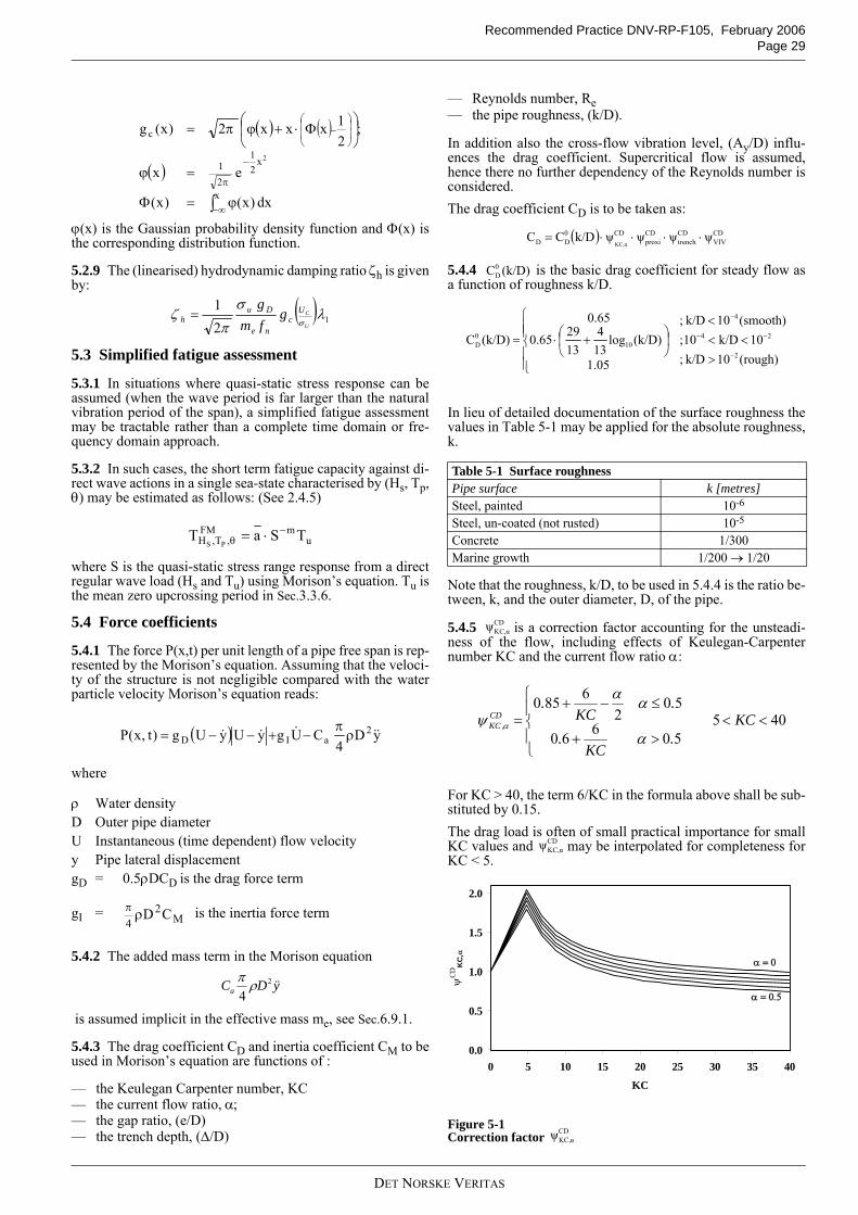
Recommended Practice DNV-RP-F105, February 2006Page 29
ϕ(x) is the Gaussian probability density function and Φ(x) isthe corresponding distribution function.
5.2.9 The (linearised) hydrodynamic damping ratio ζh is givenby:
5.3 Simplified fatigue assessment
5.3.1 In situations where quasi-static stress response can beassumed (when the wave period is far larger than the naturalvibration period of the span), a simplified fatigue assessmentmay be tractable rather than a complete time domain or fre-quency domain approach.
5.3.2 In such cases, the short term fatigue capacity against di-rect wave actions in a single sea-state characterised by (Hs, Tp,θ) may be estimated as follows: (See 2.4.5)
where S is the quasi-static stress range response from a directregular wave load (Hs and Tu) using Morison’s equation. Tu isthe mean zero upcrossing period in Sec.3.3.6.
5.4 Force coefficients
5.4.1 The force P(x,t) per unit length of a pipe free span is rep-resented by the Morison’s equation. Assuming that the veloci-ty of the structure is not negligible compared with the waterparticle velocity Morison’s equation reads:
where
5.4.2 The added mass term in the Morison equation
is assumed implicit in the effective mass me, see Sec.6.9.1.
5.4.3 The drag coefficient CD and inertia coefficient CM to beused in Morison’s equation are functions of :
— the Keulegan Carpenter number, KC— the current flow ratio, α;— the gap ratio, (e/D)— the trench depth, (∆/D)
— Reynolds number, Re— the pipe roughness, (k/D).
In addition also the cross-flow vibration level, (Ay/D) influ-ences the drag coefficient. Supercritical flow is assumed,hence there no further dependency of the Reynolds number isconsidered.The drag coefficient CD is to be taken as:
5.4.4 is the basic drag coefficient for steady flow asa function of roughness k/D.
In lieu of detailed documentation of the surface roughness thevalues in Table 5-1 may be applied for the absolute roughness,k.
Note that the roughness, k/D, to be used in 5.4.4 is the ratio be-tween, k, and the outer diameter, D, of the pipe.
5.4.5 is a correction factor accounting for the unsteadi-ness of the flow, including effects of Keulegan-Carpenternumber KC and the current flow ratio α:
For KC > 40, the term 6/KC in the formula above shall be sub-stituted by 0.15.The drag load is often of small practical importance for smallKC values and may be interpolated for completeness forKC < 5.
Figure 5-1Correction factor
ρ Water densityD Outer pipe diameterU Instantaneous (time dependent) flow velocityy Pipe lateral displacement gD = 0.5ρDCD is the drag force term
gI = is the inertia force term
( ) ( )
( )
∫ ∞−
−
π
⎟⎟
⎠
⎞
⎜⎜
⎝
⎛−
ϕ=Φ
=ϕ
⎟⎠
⎞⎜⎝
⎛ Φ⋅+ϕπ=
x
x21
21
c
dx)x()x(
ex
;21xxx2)x(g
2
( ) 121 λ
σ
πζ
σU
CUc
ne
Duh g
fmg
=
umFM
,T,H TSaTPS
−θ ⋅=
( ) yD4
CUgyUyUg)t,x(P 2aID &&&&& ρ
π−+−−=
M2
4CDρπ
ÿDCa2
4ρπ
Table 5-1 Surface roughnessPipe surface k [metres]Steel, painted 10-6
Steel, un-coated (not rusted) 10-5
Concrete 1/300Marine growth 1/200 → 1/20
( ) CDVIV
CDtrench
CDproxi
CD0DD ψψψψk/DCC
αKC,⋅⋅⋅⋅=
(k/D)C0D
(rough)10k/D10k/D10
(smooth)10k/D
;;;
1.05
(k/D)log134
13290.65
0.65
(k/D)C2
24
4
100D
−
−−
−
><<
<
⎪⎪⎩
⎪⎪⎨
⎧
⎟⎠⎞
⎜⎝⎛ +⋅=
CDαKC,ψ
40550660
502
6850<<
⎪⎩
⎪⎨
⎧
>+
≤−+= KC
.KC
.
.KC
.CD
,KC
α
αα
ψ α
CDαKC,ψ
0.0
0.5
1.0
1.5
2.0
0 5 10 15 20 25 30 35 40
KC
ψC
DK
C,α
α = 0
α = 0.5
CDαKC,ψ
DET NORSKE VERITAS
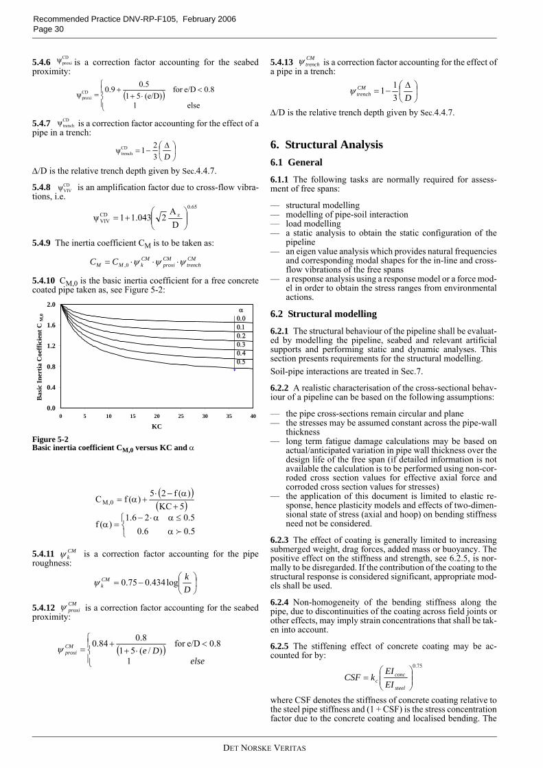
Recommended Practice DNV-RP-F105, February 2006 Page 30
5.4.6 is a correction factor accounting for the seabedproximity:
5.4.7 is a correction factor accounting for the effect of apipe in a trench:
∆/D is the relative trench depth given by Sec.4.4.7.
5.4.8 is an amplification factor due to cross-flow vibra-tions, i.e.
5.4.9 The inertia coefficient CM is to be taken as:
5.4.10 CM,0 is the basic inertia coefficient for a free concretecoated pipe taken as, see Figure 5-2:
Figure 5-2Basic inertia coefficient CM,0 versus KC and α
5.4.11 is a correction factor accounting for the piperoughness:
5.4.12 is a correction factor accounting for the seabedproximity:
5.4.13 is a correction factor accounting for the effect ofa pipe in a trench:
∆/D is the relative trench depth given by Sec.4.4.7.
6. Structural Analysis6.1 General
6.1.1 The following tasks are normally required for assess-ment of free spans:
— structural modelling— modelling of pipe-soil interaction— load modelling— a static analysis to obtain the static configuration of the
pipeline— an eigen value analysis which provides natural frequencies
and corresponding modal shapes for the in-line and cross-flow vibrations of the free spans
— a response analysis using a response model or a force mod-el in order to obtain the stress ranges from environmentalactions.
6.2 Structural modelling
6.2.1 The structural behaviour of the pipeline shall be evaluat-ed by modelling the pipeline, seabed and relevant artificialsupports and performing static and dynamic analyses. Thissection presents requirements for the structural modelling.Soil-pipe interactions are treated in Sec.7.
6.2.2 A realistic characterisation of the cross-sectional behav-iour of a pipeline can be based on the following assumptions:
— the pipe cross-sections remain circular and plane— the stresses may be assumed constant across the pipe-wall
thickness— long term fatigue damage calculations may be based on
actual/anticipated variation in pipe wall thickness over thedesign life of the free span (if detailed information is notavailable the calculation is to be performed using non-cor-roded cross section values for effective axial force andcorroded cross section values for stresses)
— the application of this document is limited to elastic re-sponse, hence plasticity models and effects of two-dimen-sional state of stress (axial and hoop) on bending stiffnessneed not be considered.
6.2.3 The effect of coating is generally limited to increasingsubmerged weight, drag forces, added mass or buoyancy. Thepositive effect on the stiffness and strength, see 6.2.5, is nor-mally to be disregarded. If the contribution of the coating to thestructural response is considered significant, appropriate mod-els shall be used.
6.2.4 Non-homogeneity of the bending stiffness along thepipe, due to discontinuities of the coating across field joints orother effects, may imply strain concentrations that shall be tak-en into account.
6.2.5 The stiffening effect of concrete coating may be ac-counted for by:
where CSF denotes the stiffness of concrete coating relative tothe steel pipe stiffness and (1 + CSF) is the stress concentrationfactor due to the concrete coating and localised bending. The
CDproxiψ
( )⎪⎩
⎪⎨⎧ <
⋅++
=else1
0.8e/Dfor (e/D)51
0.50.9ψCDproxi
CDtrenchψ
⎟⎠
⎞⎜⎝
⎛ ∆−=
D321ψCD
trench
CDVIVψ
0.65zCD
VIV DA
21.0431ψ ⎟⎟⎠
⎞⎜⎜⎝
⎛+=
CMtrench
CMproxi
CMkMM CC ψψψ ⋅⋅⋅= 0,
0.0
0.4
0.8
1.2
1.6
2.0
0 5 10 15 20 25 30 35 40
KC
Bas
ic In
ertia
Coe
ffic
ient
CM
,0
α 0.0 0.1 0.2 0.3 0.4 0.5
( )( )
⎩⎨⎧
α≤αα⋅−
=α
+α−⋅
+α=
5.06.05.026.1
)(f
5KC)(f25)(fC 0,M
f
CMkψ
⎟⎠⎞
⎜⎝⎛−=
DkCM
k log434.075.0ψ
CMproxiψ
( )⎪⎩
⎪⎨⎧ <
⋅++
=else
DeCMproxi
1
8.0e/Dfor )/(51
8.084.0ψ
CMtrenchψ
⎟⎠⎞
⎜⎝⎛ ∆
−=D
CMtrench 3
11ψ
75.0
⎟⎟⎠
⎞⎜⎜⎝
⎛=
steel
concc EI
EIkCSF
DET NORSKE VERITAS
Recommended Practice DNV-RP-F105, February 2006Page 31
parameter kc is an empirical constant accounting for the defor-mation/slippage in the corrosion coating and the cracking ofthe concrete coating. The value of kc may be taken as 0.33 forasphalt and 0.25 for PP/PE coating.In case the increased stiffness effect is utilised, the increasedbending stresses due to field joints must also be accounted for.The CSF given above is assumed valid for all relevant pipe di-ameters, D/t-ratios and concrete strengths, fcn, provided thatthat the pipe joint length exceeds 12 m, the field joint length is0.5-1.0m and the concrete coating thickness does not exceed150 mm.
6.2.6 In lieu of detailed data, it is conservative to assume thata girth weld is present in the most heavily loaded cross-section.This is also a basis for the concrete stiffening effect givenabove.
6.2.7 The cross-sectional bending stiffness of the concretecoating, EIconc, is the initial, uncracked stiffness. Young’smodulus for concrete may be taken as:
where fcn is the construction strength of the concrete. BothEconc and fcn are to be in N/mm2.
6.2.8 The boundary conditions applied at the ends of the pipelinesection modelled shall adequately represent the pipe-soil interac-tion and the continuity of the pipeline. Sufficient lengths of thepipeline at both sides of the span must be included in the modelto account for the effects of side spans, if relevant.
6.2.9 The element length to be used in a finite element modelis dictated by the accuracy required. If the stress ranges are tobe derived from the mode shapes, see 6.7.4, the accuracy of thestress ranges becomes strongly affected by the element length,especially at the span shoulders.Ideally the maximum element length should be found by re-ducing the length until the results (natural frequencies andstresses) converge towards constant values. In practice thismay be difficult to perform, and, as guidance, the elementlength should be in the order of the outer diameter of the pipe-line (1D). However, higher order modes and/or short spans (L/Ds < 30) may require shorter elements.
6.2.10 In order to obtain realistic rotational pipe-soil stiffness,contact should be ensured between at least two nodes at eachspan shoulder by using a sufficiently short element length orby other means.
6.2.11 Structural damping is due to internal friction forces ofthe pipe material and depends on the strain level and associateddeflections. If no information is available, a structural modaldamping ratio of
ζstr = 0.005can be assumed. If concrete coating is present, the sliding at theinterface between concrete and corrosion coating may furtherincrease the damping to typically 0.01 - 0.02.
6.2.12 It is recommended to verify the finite element model-ling and the post-processing by comparing the results from thefinite element analysis with the approximate response quanti-ties of 6.7 for a single span with zero effective axial force andL/Ds = 60. The in-line and cross-flow natural frequencies andstress ranges shall show similar values within ±5%.
6.2.13 ULS conditions may require a more refined pipe-soilmodelling than the linearised eigen value analysis due to po-tential sliding at the span supports.
6.3 Functional loads
6.3.1 The functional loads which shall be considered are:
— weight of the pipe and internal fluid— external and internal fluid pressure— thermal expansion and contraction — residual installation forces.
6.3.2 Response calculations must account for the relevant se-quence of load application, if important.
6.4 Static analysis
6.4.1 The static configuration is to be determined for the fol-lowing conditions if relevant:
— as-laid condition— flooded condition— pressure test condition— operating condition.
6.4.2 The static analysis should normally account for non-lin-ear effects such as:
— large displacements (geometric non-linearity)— soil non-linear response— loading sequence.
6.4.3 The stiffness of the pipeline consists of material stiffnessand geometrical stiffness. The geometrical stiffness is gov-erned by the effective axial force, Seff. This force is equal to thetrue steel wall axial force, Ntr, with corrections for the effect ofexternal and internal pressures:
The effective axial force in a span is difficult to estimate due touncertainties in operational temperature and pressure, residuallay tension and axial force relaxation by sagging, axial sliding(feed-in), lateral buckling, multi-spanning and significant sea-bed unevenness. All these effects should be considered andtaken into account if relevant. The most reliable method to es-timate the effective axial force is use of non-linear FE analysis.As boundary values, the effective axial force for a completelyunrestrained (axially) pipe becomes:
while for a totally restrained pipe the following effective axialforce applies (if pipe considered thin-walled):
3.010000 cnconc fE ⋅=
Ntr “True” steel wall axial forcepi Internal pressure pe External pressure Ai Internal cross section area of the pipe Ae External cross section area of the steel pipe
Heff Effective lay tension∆pi Internal pressure difference relative to laying,
see DNV-OS-F101As Pipe steel cross section area∆T Temperature difference relative to layingαe Temperature expansion coefficient, may be tem-
perature dependent
eeiitreff ApApNS +−=
0=effS
esiieff TEA)21(ApH αν ∆−−∆−=effS
DET NORSKE VERITAS
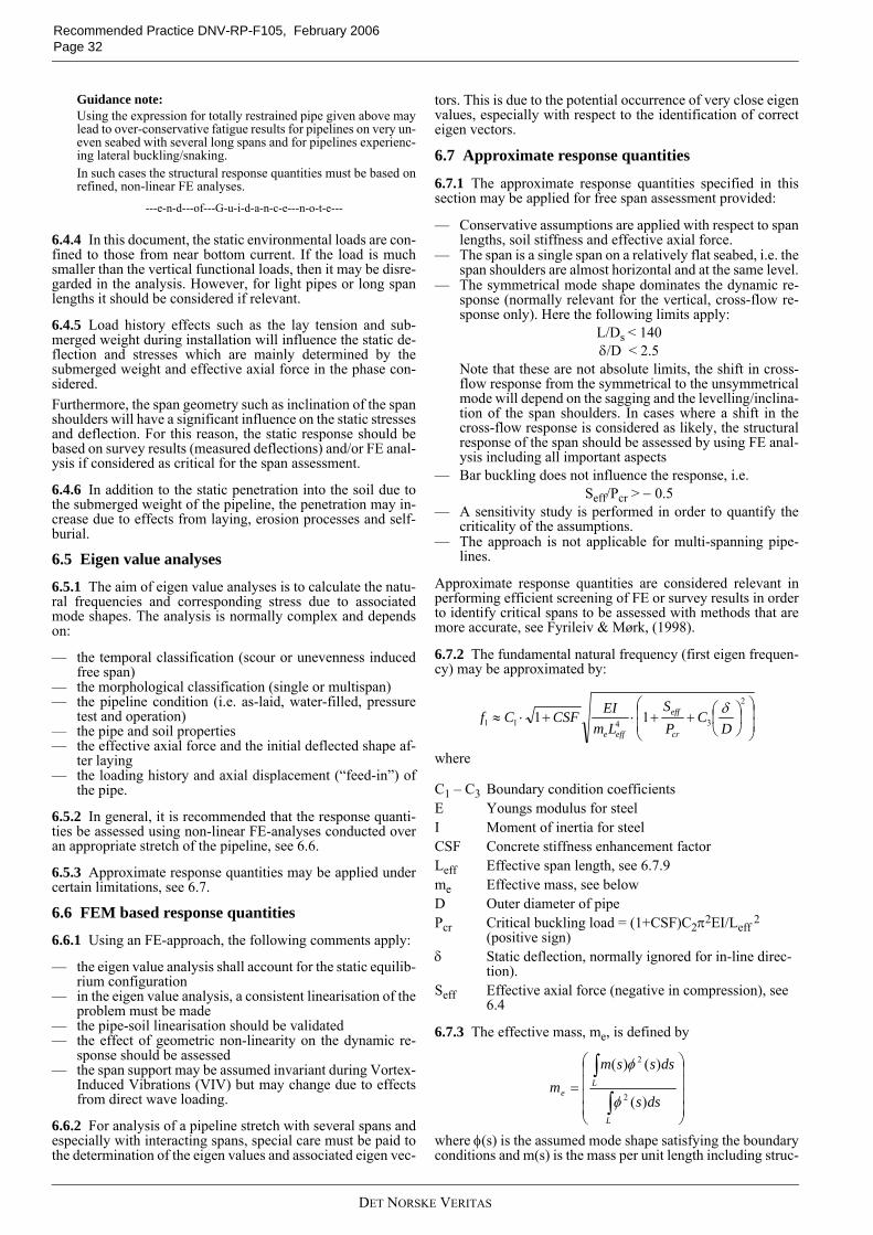
Recommended Practice DNV-RP-F105, February 2006 Page 32
Guidance note:Using the expression for totally restrained pipe given above maylead to over-conservative fatigue results for pipelines on very un-even seabed with several long spans and for pipelines experienc-ing lateral buckling/snaking.In such cases the structural response quantities must be based onrefined, non-linear FE analyses.
---e-n-d---of---G-u-i-d-a-n-c-e---n-o-t-e---
6.4.4 In this document, the static environmental loads are con-fined to those from near bottom current. If the load is muchsmaller than the vertical functional loads, then it may be disre-garded in the analysis. However, for light pipes or long spanlengths it should be considered if relevant.
6.4.5 Load history effects such as the lay tension and sub-merged weight during installation will influence the static de-flection and stresses which are mainly determined by thesubmerged weight and effective axial force in the phase con-sidered.Furthermore, the span geometry such as inclination of the spanshoulders will have a significant influence on the static stressesand deflection. For this reason, the static response should bebased on survey results (measured deflections) and/or FE anal-ysis if considered as critical for the span assessment.
6.4.6 In addition to the static penetration into the soil due tothe submerged weight of the pipeline, the penetration may in-crease due to effects from laying, erosion processes and self-burial.
6.5 Eigen value analyses
6.5.1 The aim of eigen value analyses is to calculate the natu-ral frequencies and corresponding stress due to associatedmode shapes. The analysis is normally complex and dependson:
— the temporal classification (scour or unevenness inducedfree span)
— the morphological classification (single or multispan)— the pipeline condition (i.e. as-laid, water-filled, pressure
test and operation)— the pipe and soil properties— the effective axial force and the initial deflected shape af-
ter laying— the loading history and axial displacement (“feed-in”) of
the pipe.
6.5.2 In general, it is recommended that the response quanti-ties be assessed using non-linear FE-analyses conducted overan appropriate stretch of the pipeline, see 6.6.
6.5.3 Approximate response quantities may be applied undercertain limitations, see 6.7.
6.6 FEM based response quantities
6.6.1 Using an FE-approach, the following comments apply:
— the eigen value analysis shall account for the static equilib-rium configuration
— in the eigen value analysis, a consistent linearisation of theproblem must be made
— the pipe-soil linearisation should be validated— the effect of geometric non-linearity on the dynamic re-
sponse should be assessed— the span support may be assumed invariant during Vortex-
Induced Vibrations (VIV) but may change due to effectsfrom direct wave loading.
6.6.2 For analysis of a pipeline stretch with several spans andespecially with interacting spans, special care must be paid tothe determination of the eigen values and associated eigen vec-
tors. This is due to the potential occurrence of very close eigenvalues, especially with respect to the identification of correcteigen vectors.
6.7 Approximate response quantities
6.7.1 The approximate response quantities specified in thissection may be applied for free span assessment provided:
— Conservative assumptions are applied with respect to spanlengths, soil stiffness and effective axial force.
— The span is a single span on a relatively flat seabed, i.e. thespan shoulders are almost horizontal and at the same level.
— The symmetrical mode shape dominates the dynamic re-sponse (normally relevant for the vertical, cross-flow re-sponse only). Here the following limits apply:
L/Ds < 140 δ/D < 2.5
Note that these are not absolute limits, the shift in cross-flow response from the symmetrical to the unsymmetricalmode will depend on the sagging and the levelling/inclina-tion of the span shoulders. In cases where a shift in thecross-flow response is considered as likely, the structuralresponse of the span should be assessed by using FE anal-ysis including all important aspects
— Bar buckling does not influence the response, i.e. Seff/Pcr > − 0.5
— A sensitivity study is performed in order to quantify thecriticality of the assumptions.
— The approach is not applicable for multi-spanning pipe-lines.
Approximate response quantities are considered relevant inperforming efficient screening of FE or survey results in orderto identify critical spans to be assessed with methods that aremore accurate, see Fyrileiv & Mørk, (1998).
6.7.2 The fundamental natural frequency (first eigen frequen-cy) may be approximated by:
where
6.7.3 The effective mass, me, is defined by
where φ(s) is the assumed mode shape satisfying the boundaryconditions and m(s) is the mass per unit length including struc-
C1 – C3 Boundary condition coefficientsE Youngs modulus for steelI Moment of inertia for steelCSF Concrete stiffness enhancement factor Leff Effective span length, see 6.7.9me Effective mass, see belowD Outer diameter of pipe Pcr Critical buckling load = (1+CSF)C2π2EI/Leff
2 (positive sign)
δ Static deflection, normally ignored for in-line direc-tion).
Seff Effective axial force (negative in compression), see 6.4
⎟⎟⎠
⎞⎜⎜⎝
⎛⎟⎠⎞
⎜⎝⎛++⋅+⋅≈
2
3411 11D
CPS
LmEICSFCf
cr
eff
effe
δ
⎟⎟⎟⎟
⎠
⎞
⎜⎜⎜⎜
⎝
⎛
=∫
∫
L
Le
dss
dsssmm
)(
)()(
2
2
φ
φ
DET NORSKE VERITAS
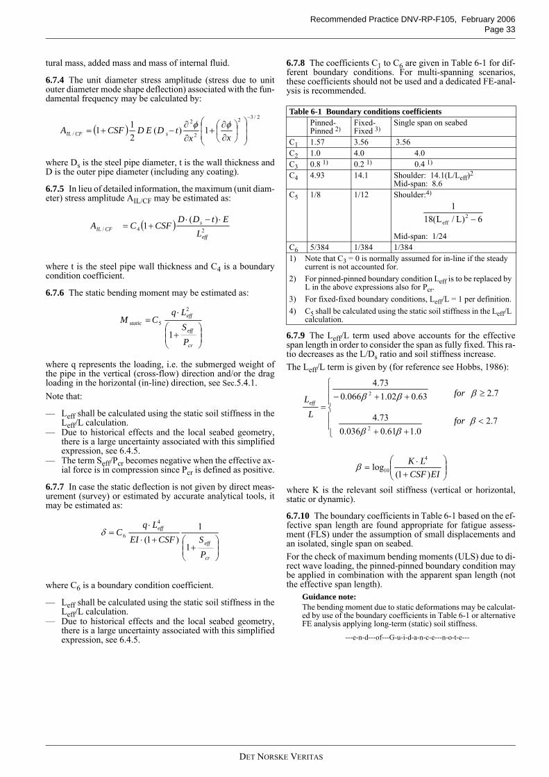
Recommended Practice DNV-RP-F105, February 2006Page 33
tural mass, added mass and mass of internal fluid.
6.7.4 The unit diameter stress amplitude (stress due to unitouter diameter mode shape deflection) associated with the fun-damental frequency may be calculated by:
where Ds is the steel pipe diameter, t is the wall thickness andD is the outer pipe diameter (including any coating).
6.7.5 In lieu of detailed information, the maximum (unit diam-eter) stress amplitude AIL/CF may be estimated as:
where t is the steel pipe wall thickness and C4 is a boundarycondition coefficient.
6.7.6 The static bending moment may be estimated as:
where q represents the loading, i.e. the submerged weight ofthe pipe in the vertical (cross-flow) direction and/or the dragloading in the horizontal (in-line) direction, see Sec.5.4.1.Note that:
— Leff shall be calculated using the static soil stiffness in theLeff/L calculation.
— Due to historical effects and the local seabed geometry,there is a large uncertainty associated with this simplifiedexpression, see 6.4.5.
— The term Seff/Pcr becomes negative when the effective ax-ial force is in compression since Pcr is defined as positive.
6.7.7 In case the static deflection is not given by direct meas-urement (survey) or estimated by accurate analytical tools, itmay be estimated as:
where C6 is a boundary condition coefficient.
— Leff shall be calculated using the static soil stiffness in theLeff/L calculation.
— Due to historical effects and the local seabed geometry,there is a large uncertainty associated with this simplifiedexpression, see 6.4.5.
6.7.8 The coefficients C1 to C6 are given in Table 6-1 for dif-ferent boundary conditions. For multi-spanning scenarios,these coefficients should not be used and a dedicated FE-anal-ysis is recommended.
6.7.9 The Leff/L term used above accounts for the effectivespan length in order to consider the span as fully fixed. This ra-tio decreases as the L/Ds ratio and soil stiffness increase. The Leff/L term is given by (for reference see Hobbs, 1986):
where K is the relevant soil stiffness (vertical or horizontal,static or dynamic).
6.7.10 The boundary coefficients in Table 6-1 based on the ef-fective span length are found appropriate for fatigue assess-ment (FLS) under the assumption of small displacements andan isolated, single span on seabed. For the check of maximum bending moments (ULS) due to di-rect wave loading, the pinned-pinned boundary condition maybe applied in combination with the apparent span length (notthe effective span length).
Guidance note:The bending moment due to static deformations may be calculat-ed by use of the boundary coefficients in Table 6-1 or alternativeFE analysis applying long-term (static) soil stiffness.
---e-n-d---of---G-u-i-d-a-n-c-e---n-o-t-e---
( )2/32
2
2
/ 1)(211
−
⎟⎟⎠
⎞⎜⎜⎝
⎛⎟⎠⎞
⎜⎝⎛
∂∂
+∂∂
−+=xx
tDEDCSFA sCFILφφ
( )24/
)(1
eff
sCFIL L
EtDDCSFCA
⋅−⋅+=
⎟⎟⎠
⎞⎜⎜⎝
⎛+
⋅=
cr
eff
effstatic
PSLq
CM1
2
5
⎟⎟⎠
⎞⎜⎜⎝
⎛+
+⋅
⋅=
cr
eff
eff
PSCSFEI
LqC
1
1)1(
4
6δ
Table 6-1 Boundary conditions coefficientsPinned-Pinned 2)
Fixed-Fixed 3)
Single span on seabed
C1 1.57 3.56 3.56C2 1.0 4.0 4.0C3 0.8 1) 0.2 1) 0.4 1)
C4 4.93 14.1 Shoulder: 14.1(L/Leff)2Mid-span: 8.6
C5 1/8 1/12 Shoulder:4)
Mid-span: 1/24C6 5/384 1/384 1/3841) Note that C3 = 0 is normally assumed for in-line if the steady
current is not accounted for.2) For pinned-pinned boundary condition Leff is to be replaced by
L in the above expressions also for Pcr.3) For fixed-fixed boundary conditions, Leff/L = 1 per definition.4) C5 shall be calculated using the static soil stiffness in the Leff/L
calculation.
6)L/L(181
2eff −
7.2
7.2
0.161.0036.073.4
63.002.1066.073.4
2
2
<
≥
⎪⎪
⎩
⎪⎪
⎨
⎧
++
++−=
β
β
ββ
ββ
for
for
LLeff
⎟⎟⎠
⎞⎜⎜⎝
⎛+
⋅=
EICSFLK
)1(log
4
10β
DET NORSKE VERITAS
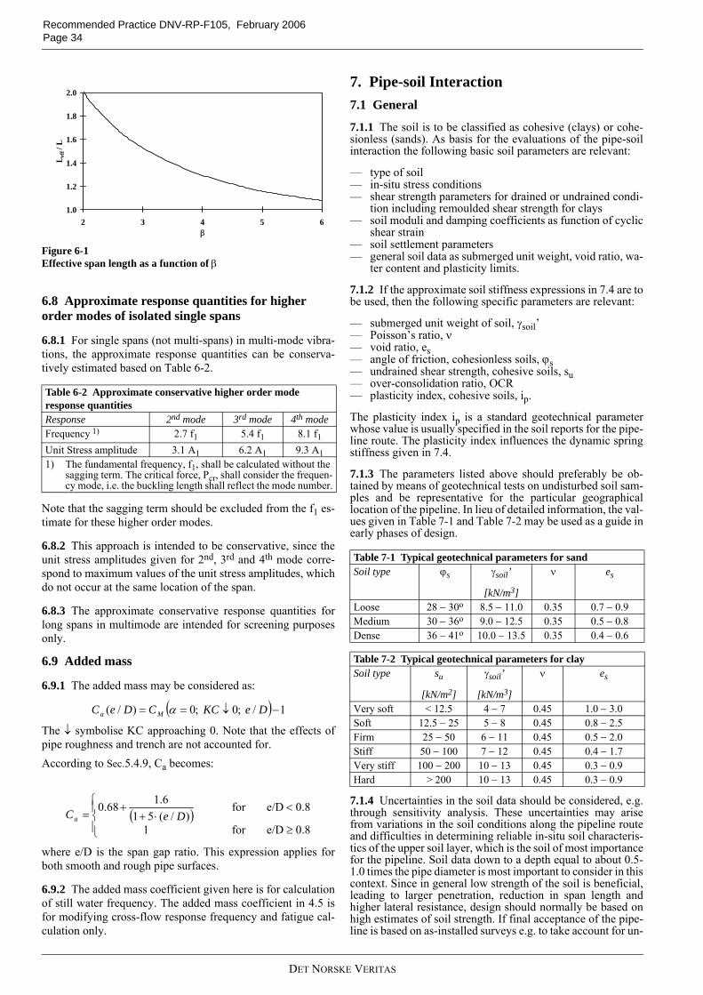
Recommended Practice DNV-RP-F105, February 2006 Page 34
Figure 6-1Effective span length as a function of β
6.8 Approximate response quantities for higher order modes of isolated single spans
6.8.1 For single spans (not multi-spans) in multi-mode vibra-tions, the approximate response quantities can be conserva-tively estimated based on Table 6-2.
Note that the sagging term should be excluded from the f1 es-timate for these higher order modes.
6.8.2 This approach is intended to be conservative, since theunit stress amplitudes given for 2nd, 3rd and 4th mode corre-spond to maximum values of the unit stress amplitudes, whichdo not occur at the same location of the span.
6.8.3 The approximate conservative response quantities forlong spans in multimode are intended for screening purposesonly.
6.9 Added mass
6.9.1 The added mass may be considered as:
The ↓ symbolise KC approaching 0. Note that the effects ofpipe roughness and trench are not accounted for.According to Sec.5.4.9, Ca becomes:
where e/D is the span gap ratio. This expression applies forboth smooth and rough pipe surfaces.
6.9.2 The added mass coefficient given here is for calculationof still water frequency. The added mass coefficient in 4.5 isfor modifying cross-flow response frequency and fatigue cal-culation only.
7. Pipe-soil Interaction7.1 General
7.1.1 The soil is to be classified as cohesive (clays) or cohe-sionless (sands). As basis for the evaluations of the pipe-soilinteraction the following basic soil parameters are relevant:
— type of soil— in-situ stress conditions— shear strength parameters for drained or undrained condi-
tion including remoulded shear strength for clays— soil moduli and damping coefficients as function of cyclic
shear strain— soil settlement parameters— general soil data as submerged unit weight, void ratio, wa-
ter content and plasticity limits.
7.1.2 If the approximate soil stiffness expressions in 7.4 are tobe used, then the following specific parameters are relevant:
— submerged unit weight of soil, γsoil’— Poisson’s ratio, ν— void ratio, es— angle of friction, cohesionless soils, ϕs— undrained shear strength, cohesive soils, su— over-consolidation ratio, OCR— plasticity index, cohesive soils, ip.
The plasticity index ip is a standard geotechnical parameterwhose value is usually specified in the soil reports for the pipe-line route. The plasticity index influences the dynamic springstiffness given in 7.4.
7.1.3 The parameters listed above should preferably be ob-tained by means of geotechnical tests on undisturbed soil sam-ples and be representative for the particular geographicallocation of the pipeline. In lieu of detailed information, the val-ues given in Table 7-1 and Table 7-2 may be used as a guide inearly phases of design.
7.1.4 Uncertainties in the soil data should be considered, e.g.through sensitivity analysis. These uncertainties may arisefrom variations in the soil conditions along the pipeline routeand difficulties in determining reliable in-situ soil characteris-tics of the upper soil layer, which is the soil of most importancefor the pipeline. Soil data down to a depth equal to about 0.5-1.0 times the pipe diameter is most important to consider in thiscontext. Since in general low strength of the soil is beneficial,leading to larger penetration, reduction in span length andhigher lateral resistance, design should normally be based onhigh estimates of soil strength. If final acceptance of the pipe-line is based on as-installed surveys e.g. to take account for un-
Table 6-2 Approximate conservative higher order mode response quantities Response 2nd mode 3rd mode 4th modeFrequency 1) 2.7 f1 5.4 f1 8.1 f1Unit Stress amplitude 3.1 A1 6.2 A1 9.3 A11) The fundamental frequency, f1, shall be calculated without the
sagging term. The critical force, Pcr, shall consider the frequen-cy mode, i.e. the buckling length shall reflect the mode number.
1.0
1.2
1.4
1.6
1.8
2.0
2 3 4 5 6β
L eff
/ L
( ) 1/;0;0)/( −↓== DeKCCDeC Ma α
( )⎪⎩
⎪⎨⎧
≥
<⋅+
+=
8.0e/Dfor 1
8.0e/Dfor )/(51
6.168.0DeCa
Table 7-1 Typical geotechnical parameters for sandSoil type ϕs γsoil’
[kN/m3]
ν es
Loose 28 − 30o 8.5 − 11.0 0.35 0.7 − 0.9Medium 30 − 36o 9.0 − 12.5 0.35 0.5 − 0.8Dense 36 − 41o 10.0 − 13.5 0.35 0.4 − 0.6
Table 7-2 Typical geotechnical parameters for claySoil type su
[kN/m2]
γsoil’
[kN/m3]
ν es
Very soft < 12.5 4 − 7 0.45 1.0 − 3.0Soft 12.5 − 25 5 − 8 0.45 0.8 − 2.5Firm 25 − 50 6 − 11 0.45 0.5 − 2.0Stiff 50 − 100 7 − 12 0.45 0.4 − 1.7Very stiff 100 − 200 10 − 13 0.45 0.3 − 0.9Hard > 200 10 − 13 0.45 0.3 − 0.9
DET NORSKE VERITAS
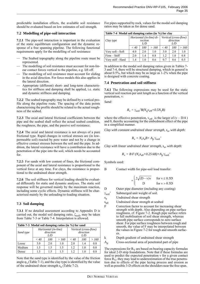
Recommended Practice DNV-RP-F105, February 2006Page 35
predictable installation effects, the available soil resistanceshould be evaluated based on low estimates of soil strength.
7.2 Modelling of pipe-soil interaction
7.2.1 The pipe-soil interaction is important in the evaluationof the static equilibrium configuration and the dynamic re-sponse of a free spanning pipeline. The following functionalrequirements apply for the modelling of soil resistance:
— The Seabed topography along the pipeline route must berepresented.
— The modelling of soil resistance must account for non-lin-ear contact forces vertical to the pipeline, e.g. lift off.
— The modelling of soil resistance must account for slidingin the axial direction. For force models this also applies inthe lateral direction.
— Appropriate (different) short- and long-term characteris-tics for stiffness and damping shall be applied, i.e. staticand dynamic stiffness and damping.
7.2.2 The seabed topography may be defined by a vertical pro-file along the pipeline route. The spacing of the data pointscharacterising the profile should be related to the actual rough-ness of the seabed.
7.2.3 The axial and lateral frictional coefficients between thepipe and the seabed shall reflect the actual seabed condition,the roughness, the pipe, and the passive soil resistance.
7.2.4 The axial and lateral resistance is not always of a purefrictional type. Rapid changes in vertical stresses are (in low-permeable soil) reacted by pore water and not by a change ineffective contact stresses between the soil and the pipe. In ad-dition, the lateral resistance will have a contribution due to thepenetration of the pipe into the soil, which needs be accountedfor.
7.2.5 For sands with low content of fines, the frictional com-ponent of the axial and lateral resistance is proportional to thevertical force at any time. For clays, the resistance is propor-tional to the undrained shear strength.
7.2.6 The soil stiffness for vertical loading should be evaluat-ed differently for static and dynamic analyses. The static soilresponse will be governed mainly by the maximum reaction,including some cyclic effects. Dynamic stiffness will be char-acterised mainly by the unloading/re-loading situation.
7.3 Soil damping
7.3.1 If no detailed assessment according to Appendix D iscarried out, the modal soil damping ratio, ζsoil, may be takenfrom Table 7-3 or Table 7-4. Interpolation is allowed.
Note that the sand type is identified by the value of the frictionangle ϕs (Table 7-1), and the clay type is identified by the valueof the undrained shear strength su (Table 7-2).
For pipes supported by rock, values for the modal soil dampingratios may be taken as for dense sand.
In addition to the modal soil damping ratios given in Tables 7-3 and 7-4, there will be structural damping, which in general isabout 0.5%, but which may be as large as 1-2% when the pipeis designed with concrete coating.
7.4 Penetration and soil stiffness
7.4.1 The following expressions may be used for the staticvertical soil reaction per unit length as a function of the verticalpenetration, v:Sand:
Rv = γsoil’B(Nqveff+0.5NγB)
where the effective penetration, veff , is the larger of (v − D/4 )and 0, thereby accounting for the embedment effect of the pipein a simplified manner.Clay with constant undrained shear strength, su, with depth:
Rv = NcsuB+ Ap·γsoil’
Clay with linear undrained shear strength, su, with depth:
Rv = B·F·(Ncsu0+0.25·kB)+Ap·γsoil’
Symbols used:
The expressions for RV are based on bearing capacity formulasfor ideal 2-D strip foundations. Note that if these formulas areused to predict the expected penetration v for a given contactforce RV, they may lead to underestimation of the true penetra-tion due to effects of the pipe laying process and erosion aswell as possible 3-D effects on the shoulders near the free span.
Table 7-3 Modal soil damping ratios (in %) for sand
Sand typeHorizontal (in-line)
directionL/D
Vertical (cross-flow) direction
L/D< 40 100 > 160 < 40 100 > 160
Loose 3.0 2.0 1.0 2.0 1.4 0.8Medium 1.5 1.5 1.5 1.2 1.0 0.8Dense 1.5 1.5 1.5 1.2 1.0 0.8
Table 7-4 Modal soil damping ratios (in %) for clay
Clay typeHorizontal (in-line) di-
rectionL/D
Vertical (cross-flow) direction
L/D< 40 100 > 160 < 40 100 > 160
Very soft - Soft 4.0 2.0 1.0 3.0 2.0 1.0Firm – Stiff 2.0 1.4 0.8 1.2 1.0 0.8Very stiff - Hard 1.4 1.0 0.6 0.7 0.6 0.5
B Contact width for pipe-soil load transfer:
D Outer pipe diameter (including any coating)γsoil’ Submerged unit weight of soil.su Undrained shear strengthsu0 Undrained shear strength at seabedF Correction factor to account for increasing shear
strength with depth. Also depending on pipe surface roughness, cf. Figure 7-2. Rough pipe surface refers to full mobilisation of soil shear strength, whereas smooth pipe surface corresponds to zero surface shear. For pipe surface roughness between rough and smooth, the value of F may be interpolated between the values in Figure 7-2 for rough and smooth surfac-es.
k Depth gradient of undrained shear strengthAp Cross-sectional area of penetrated part of pipe
⎪⎩
⎪⎨⎧
>≤−=
0.5Dfor v D0.5Dfor v v)vD(2
DET NORSKE VERITAS
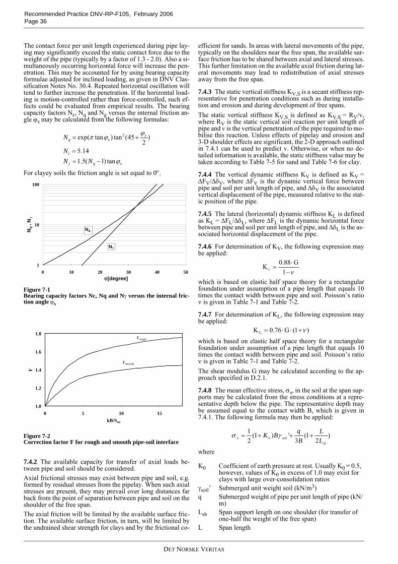
Recommended Practice DNV-RP-F105, February 2006 Page 36
The contact force per unit length experienced during pipe lay-ing may significantly exceed the static contact force due to theweight of the pipe (typically by a factor of 1.3 - 2.0). Also a si-multaneously occurring horizontal force will increase the pen-etration. This may be accounted for by using bearing capacityformulae adjusted for inclined loading, as given in DNV Clas-sification Notes No. 30.4. Repeated horizontal oscillation willtend to further increase the penetration. If the horizontal load-ing is motion-controlled rather than force-controlled, such ef-fects could be evaluated from empirical results. The bearingcapacity factors Nc, Nq and Ng versus the internal friction an-gle ϕs may be calculated from the following formulas:
For clayey soils the friction angle is set equal to 0°.
Figure 7-1Bearing capacity factors Nc, Nq and Nγ versus the internal fric-tion angle ϕs
Figure 7-2Correction factor F for rough and smooth pipe-soil interface
7.4.2 The available capacity for transfer of axial loads be-tween pipe and soil should be considered.Axial frictional stresses may exist between pipe and soil, e.g.formed by residual stresses from the pipelay. When such axialstresses are present, they may prevail over long distances farback from the point of separation between pipe and soil on theshoulder of the free span. The axial friction will be limited by the available surface fric-tion. The available surface friction, in turn, will be limited bythe undrained shear strength for clays and by the frictional co-
efficient for sands. In areas with lateral movements of the pipe,typically on the shoulders near the free span, the available sur-face friction has to be shared between axial and lateral stresses.This further limitation on the available axial friction during lat-eral movements may lead to redistribution of axial stressesaway from the free span.
7.4.3 The static vertical stiffness KV,S is a secant stiffness rep-resentative for penetration conditions such as during installa-tion and erosion and during development of free spans. The static vertical stiffness KV,S is defined as KV,S = RV/v,where RV is the static vertical soil reaction per unit length ofpipe and v is the vertical penetration of the pipe required to mo-bilise this reaction. Unless effects of pipelay and erosion and3-D shoulder effects are significant, the 2-D approach outlinedin 7.4.1 can be used to predict v. Otherwise, or when no de-tailed information is available, the static stiffness value may betaken according to Table 7-5 for sand and Table 7-6 for clay.
7.4.4 The vertical dynamic stiffness KV is defined as KV =∆FV/∆δV, where ∆FV is the dynamic vertical force betweenpipe and soil per unit length of pipe, and ∆δV is the associatedvertical displacement of the pipe, measured relative to the stat-ic position of the pipe.
7.4.5 The lateral (horizontal) dynamic stiffness KL is definedas KL = ∆FL/∆δL, where ∆FL is the dynamic horizontal forcebetween pipe and soil per unit length of pipe, and ∆δL is the as-sociated horizontal displacement of the pipe.
7.4.6 For determination of KV, the following expression maybe applied:
which is based on elastic half space theory for a rectangularfoundation under assumption of a pipe length that equals 10times the contact width between pipe and soil. Poisson’s ratioν is given in Table 7-1 and Table 7-2.
7.4.7 For determination of KL, the following expression maybe applied:
which is based on elastic half space theory for a rectangularfoundation under assumption of a pipe length that equals 10times the contact width between pipe and soil. Poisson’s ratioν is given in Table 7-1 and Table 7-2.The shear modulus G may be calculated according to the ap-proach specified in D.2.1.
7.4.8 The mean effective stress, σs, in the soil at the span sup-ports may be calculated from the stress conditions at a repre-sentative depth below the pipe. The representative depth maybe assumed equal to the contact width B, which is given in7.4.1. The following formula may then be applied:
where
sq
c
ssq
NNN
N
ϕ
ϕϕπ
γ tan)1(5.114.5
)2
45(tan)tanexp( 2
−==
+=
1
10
100
0 10 20 30 40 50ϕ[degree]
Nq ,
Nγ
Nγ
Nq
1.0
1.2
1.4
1.6
1.8
0 5 10 15kB/Suo
F
Fsmooth
Frough
K0 Coefficient of earth pressure at rest. Usually K0 = 0.5, however, values of K0 in excess of 1.0 may exist for clays with large over-consolidation ratios
γsoil’ Submerged unit weight soil (kN/m3)q Submerged weight of pipe per unit length of pipe (kN/
m)Lsh Span support length on one shoulder (for transfer of
one-half the weight of the free span)L Span length
ν−⋅
=1
G88.0K v
)1(G76.0K L ν+⋅⋅=
)2
1(3
')1(21
0sh
soilS LL
BqBK +++= γσ
DET NORSKE VERITAS
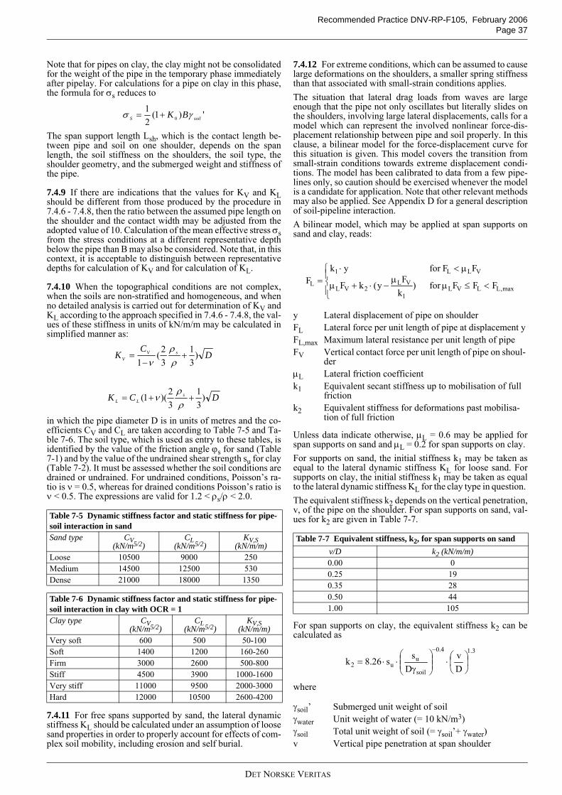
Recommended Practice DNV-RP-F105, February 2006Page 37
Note that for pipes on clay, the clay might not be consolidatedfor the weight of the pipe in the temporary phase immediatelyafter pipelay. For calculations for a pipe on clay in this phase,the formula for σs reduces to
The span support length Lsh, which is the contact length be-tween pipe and soil on one shoulder, depends on the spanlength, the soil stiffness on the shoulders, the soil type, theshoulder geometry, and the submerged weight and stiffness ofthe pipe.
7.4.9 If there are indications that the values for KV and KLshould be different from those produced by the procedure in7.4.6 - 7.4.8, then the ratio between the assumed pipe length onthe shoulder and the contact width may be adjusted from theadopted value of 10. Calculation of the mean effective stress σsfrom the stress conditions at a different representative depthbelow the pipe than B may also be considered. Note that, in thiscontext, it is acceptable to distinguish between representativedepths for calculation of KV and for calculation of KL.
7.4.10 When the topographical conditions are not complex,when the soils are non-stratified and homogeneous, and whenno detailed analysis is carried out for determination of KV andKL according to the approach specified in 7.4.6 - 7.4.8, the val-ues of these stiffness in units of kN/m/m may be calculated insimplified manner as:
in which the pipe diameter D is in units of metres and the co-efficients CV and CL are taken according to Table 7-5 and Ta-ble 7-6. The soil type, which is used as entry to these tables, isidentified by the value of the friction angle ϕs for sand (Table7-1) and by the value of the undrained shear strength su for clay(Table 7-2). It must be assessed whether the soil conditions aredrained or undrained. For undrained conditions, Poisson’s ra-tio is ν = 0.5, whereas for drained conditions Poisson’s ratio isν < 0.5. The expressions are valid for 1.2 < ρs/ρ < 2.0.
7.4.11 For free spans supported by sand, the lateral dynamicstiffness KL should be calculated under an assumption of loosesand properties in order to properly account for effects of com-plex soil mobility, including erosion and self burial.
7.4.12 For extreme conditions, which can be assumed to causelarge deformations on the shoulders, a smaller spring stiffnessthan that associated with small-strain conditions applies. The situation that lateral drag loads from waves are largeenough that the pipe not only oscillates but literally slides onthe shoulders, involving large lateral displacements, calls for amodel which can represent the involved nonlinear force-dis-placement relationship between pipe and soil properly. In thisclause, a bilinear model for the force-displacement curve forthis situation is given. This model covers the transition fromsmall-strain conditions towards extreme displacement condi-tions. The model has been calibrated to data from a few pipe-lines only, so caution should be exercised whenever the modelis a candidate for application. Note that other relevant methodsmay also be applied. See Appendix D for a general descriptionof soil-pipeline interaction.A bilinear model, which may be applied at span supports onsand and clay, reads:
Unless data indicate otherwise, µL = 0.6 may be applied forspan supports on sand and µL = 0.2 for span supports on clay. For supports on sand, the initial stiffness k1 may be taken asequal to the lateral dynamic stiffness KL for loose sand. Forsupports on clay, the initial stiffness k1 may be taken as equalto the lateral dynamic stiffness KL for the clay type in question. The equivalent stiffness k2 depends on the vertical penetration,v, of the pipe on the shoulder. For span supports on sand, val-ues for k2 are given in Table 7-7.
For span supports on clay, the equivalent stiffness k2 can becalculated as
where
Table 7-5 Dynamic stiffness factor and static stiffness for pipe-soil interaction in sandSand type CV
(kN/m5/2)CL
(kN/m5/2)KV,S
(kN/m/m)Loose 10500 9000 250Medium 14500 12500 530Dense 21000 18000 1350
Table 7-6 Dynamic stiffness factor and static stiffness for pipe-soil interaction in clay with OCR = 1Clay type CV
(kN/m5/2)CL
(kN/m5/2)KV,S
(kN/m/m)Very soft 600 500 50-100Soft 1400 1200 160-260Firm 3000 2600 500-800Stiff 4500 3900 1000-1600Very stiff 11000 9500 2000-3000Hard 12000 10500 2600-4200
')1(21
0 soilS BK γσ +=
DC
K sVV )
31
32(
1+
−=
ρρ
ν
DCK sLL )
31
32)(1( ++=
ρρ
ν
y Lateral displacement of pipe on shoulderFL Lateral force per unit length of pipe at displacement yFL,max Maximum lateral resistance per unit length of pipeFV Vertical contact force per unit length of pipe on shoul-
derµL Lateral friction coefficientk1 Equivalent secant stiffness up to mobilisation of full
frictionk2 Equivalent stiffness for deformations past mobilisa-
tion of full friction
Table 7-7 Equivalent stiffness, k2, for span supports on sandv/D k2 (kN/m/m)0.00 00.25 190.35 280.50 441.00 105
γsoil’ Submerged unit weight of soilγwater Unit weight of water (= 10 kN/m3)γsoil Total unit weight of soil (= γsoil’+ γwater)v Vertical pipe penetration at span shoulder
⎪⎩
⎪⎨⎧
<≤µµ
−⋅+µ
µ<⋅=
max,LLVL1
VL2VL
VLL1
L FFFfor )kFy(kF
FFfor ykF
3.14.0
soil
uu2 D
vD
ss26.8k ⎟⎠⎞
⎜⎝⎛⋅⎟⎟
⎠
⎞⎜⎜⎝
⎛γ
⋅⋅=−
DET NORSKE VERITAS
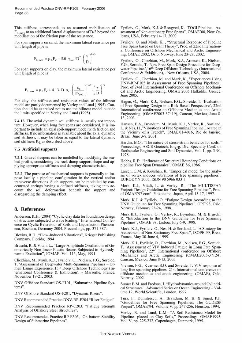
Recommended Practice DNV-RP-F105, February 2006 Page 38
This stiffness corresponds to an assumed mobilisation ofFL,max at an additional lateral displacement of D/2 beyond themobilisation of the friction part of the resistance.For span supports on sand, the maximum lateral resistance perunit length of pipe is
For span supports on clay, the maximum lateral resistance perunit length of pipe is
For clay, the stiffness and resistance values of the bilinearmodel are partly documented by Verley and Lund (1995). Cau-tion should be exercised not to use the bilinear model outsidethe limits specified in Verley and Lund (1995).
7.4.13 The axial dynamic soil stiffness is usually not impor-tant. However, when long free spans are considered, it is im-portant to include an axial soil-support model with friction andstiffness. If no information is available about the axial dynamicsoil stiffness, it may be taken as equal to the lateral dynamicsoil stiffness KL as described above.
7.5 Artificial supports
7.5.1 Gravel sleepers can be modelled by modifying the sea-bed profile, considering the rock dump support shape and ap-plying appropriate stiffness and damping characteristics.
7.5.2 The purpose of mechanical supports is generally to im-pose locally a pipeline configuration in the vertical and/ortransverse directions. Such supports can be modelled by con-centrated springs having a defined stiffness, taking into ac-count the soil deformation beneath the support anddisregarding the damping effect.
8. ReferencesAndersen, K.H. (2004) “Cyclic clay data for foundation designof structures subjected to wave loading.” International Confer-ence on Cyclic Behaviour of Soils and Liquefaction Phenom-ena, Bochum, Germany 2004. Proceedings, pp. 371-387.Blevins, R.D., “Flow-Induced Vibrations”, Krieger PublishingCompany, Florida, 1994Bruschi, R. & Vitali, L., “Large-Amplitude Oscillations of Ge-ometrically Non-linear Elastic Beams Subjected to Hydrody-namic Excitation”, JOMAE, Vol. 113, May, 1991.Chezhian, M., Mørk, K.J., Fyrileiv, O., Nielsen, F.G., Søreide,T. 'Assessment of Deepwater Multi-Spanning Pipelines – Or-men Lange Experience',15th Deep Offshore Technology (In-ternational Conference & Exhibition), - Marseille, France,November 19-21, 2003.DNV Offshore Standard OS-F101, “Submarine Pipeline Sys-tems”. DNV Offshore Standard OS-F201, “Dynamic Risers”. DNV Recommended Practice DNV-RP-F204 “Riser Fatigue”.DNV Recommended Practice RP-C203, “Fatigue StrengthAnalysis of Offshore Steel Structures”.DNV Recommended Practice RP-E305, “On-bottom StabilityDesign of Submarine Pipelines”.
Fyrileiv, O., Mørk, K.J. & Rongved, K. “TOGI Pipeline – As-sessment of Non-stationary Free Spans”, OMAE’00, New Or-leans, USA, February 14-17, 2000.Fyrileiv, O. and Mørk, K. , “Structural Response of PipelineFree Spans based on Beam Theory”, Proc. of 22nd Internation-al Conference on Offshore Mechanical and Arctic Engineer-ing, OMAE 2002, Oslo, Norway, June 23-28, 2002.Fyrileiv, O., Chezhian, M., Mørk, K.J., Arnesen, K., Nielsen,F.G., Søreide, T. 'New Free Span Design Procedure for Deep-water Pipelines',16th Deep Offshore Technology (InternationalConference & Exhibition), - New Orleans, USA, 2004.Fyrileiv, O., Chezhian, M. and Mørk, K., "Experiences UsingDNV-RP-F105 in Assessment of Free Spanning Pipelines",Proc. of 24rd International Conference on Offshore Mechani-cal and Arctic Engineering, OMAE 2005 Halkidiki, Greece,June 2005.Hagen, Ø., Mørk, K.J., Nielsen, F.G., Søreide, T. ‘Evaluationof Free Spanning Design in a Risk Based Perspective’, 22ndInternational conference on Offshore Mechanics and ArcticEngineering, (OMAE2003-37419), Cancun, Mexico, June 8-13, 2003.Hansen, E.A., Bryndum, M., Mørk, K.J., Verley, R., Sortland,L. & Nes, H.,”Vibrations of Free Spanning Pipeline Located inthe Vicinity of a Trench", OMAE'01-4016, Rio de Janeiro,Brazil, June 3-8, 2001.Hardin, B.O., “The nature of stress-strain behavior for soils,”Proceedings, ASCE Geotech. Engrg. Div. Specialty Conf. onEarthquake Engineering and Soil Dynamics, Vol. 1, pp. 3-90,1978. Hobbs, R.E:, “Influence of Structural Boundary Conditions onpipeline Free Span Dynamics”, OMAE’86, 1986.Larsen, C.M, & Koushan, K. ”Emperical model for the analy-sis of vortex induces vibrations of free spanning pipelines”,EURODYN 2005, ISBN 90 5966 033 1Mørk, K.J., Vitali, L. & Verley, R., “The MULTISPANProject: Design Guideline for Free Spanning Pipelines”, Proc.of OMAE’97 conf., Yokohama, Japan, April 13-17, 1997.Mørk, K.J. & Fyrileiv, O. “Fatigue Design According to theDNV Guideline for Free Spanning Pipelines”, OPT’98, Oslo,Norway, February 23-24, 1998.Mørk K.J., Fyrileiv, O., Verley, R., Bryndum, M. & Bruschi,R. “Introduction to the DNV Guideline for Free SpanningPipelines”, OMAE’98, Lisboa, July 6-9, 1998.Mørk, K.J., Fyrileiv, O., Nes, H. & Sortland, L. “A Strategy forAssessment of Non-Stationary Free Spans”, ISOPE-99, Brest,France, May 30-June 4, 1999.Mørk, K.J., Fyrileiv, O., Chezhian, M., Nielsen, F.G., Søreide,T. ‘Assessment of VIV Induced Fatigue in Long Free Span-ning Pipelines’, 22nd International conference on OffshoreMechanics and Arctic Engineering, (OMAE2003-37124),Cancun, Mexico, June 8-13, 2003.Nielsen, F.G., Kvarme, S.O. and Søreide, T. VIV response oflong free spanning pipelines. 21st International conference onoffshore mechanics and arctic engineering, (OMAE), Oslo,Norway, 2002.Sumer B.M. and Fredsøe, J. “Hydrodynamics around Cylindri-cal Structures”, Advanced Series on Ocean Engineering – Vol-ume 12, World Scientific, London, 1997.Tura, F., Dumitrescu, A., Bryndum, M. B. & Smed, P.F.“Guidelines for Free Spanning Pipelines: The GUDESPProject”, OMAE’94, Volume V, pp 247-256, Houston, 1994.Verley, R. and Lund, K.M., “A Soil Resistance Model forPipelines placed on Clay Soils,” Proceedings, OMAE1995,Vol. V, pp. 225-232, Copenhagen, Denmark, 1995.
25.12
soilVLmax,L DvD'0.5FF ⎟
⎠⎞
⎜⎝⎛⋅⋅γ⋅+µ=
3.14.0
soil
uuVLmax,L D
vD
ssD13.4FF ⎟⎠⎞
⎜⎝⎛⋅⎟⎟
⎠
⎞⎜⎜⎝
⎛γ
⋅⋅⋅+µ=−
DET NORSKE VERITAS
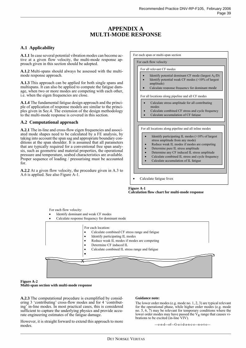
Recommended Practice DNV-RP-F105, February 2006Page 39
APPENDIX A MULTI-MODE RESPONSE
A.1 Applicability
A.1.1 In case several potential vibration modes can become ac-tive at a given flow velocity, the multi-mode response ap-proach given in this section should be adopted.
A.1.2 Multi-spans should always be assessed with the multi-mode response approach.
A.1.3 This approach can be applied for both single spans andmultispans. It can also be applied to compute the fatigue dam-age, when two or more modes are competing with each other,i.e. when the eigen frequencies are close.
A.1.4 The fundamental fatigue design approach and the princi-ple of application of response models are similar to the princi-ples given in Sec.4. The extension of the design methodologyto the multi-mode response is covered in this section.
A.2 Computational approach
A.2.1 The in-line and cross-flow eigen frequencies and associ-ated mode shapes need to be calculated by a FE analysis, bytaking into account the span sag and appropriate boundary con-ditions at the span shoulder. It is assumed that all parametersthat are typically required for a conventional free span analy-sis, such as geometric and material properties, the operationalpressure and temperature, seabed characteristics are available.Proper sequence of loading / pressurising must be accountedfor.
A.2.2 At a given flow velocity, the procedure given in A.3 toA.6 is applied. See also Figure A-1.
Figure A-1 Calculation flow chart for multi-mode response
Figure A-2 Multi-span section with multi-mode response
A.2.3 The computational procedure is exemplified by consid-ering 3 ‘contributing’ cross-flow modes and for 4 ‘contribut-ing’ in-line modes. In most practical cases, this is consideredsufficient to capture the underlying physics and provide accu-rate engineering estimates of the fatigue damage.However, it is straight forward to extend this approach to moremodes.
Guidance note:The lower order modes (e.g. mode no. 1, 2, 3) are typical relevantfor the operational phase, while higher order modes (e.g. modeno. 5, 6, 7) may be relevant for temporary conditions where thelower order modes may have passed the VR range that causes vi-brations to be excited (in-line VIV).
---e-n-d---of---G-u-i-d-a-n-c-e---n-o-t-e---
For each span or multi-span section • Calculate fatigue lives
For each flow velocity
For all relevant CF modes For all locations along pipeline and all CF modes
• Identify potential dominant CF mode (largest AZ/D) • Identify potential weak CF modes (>10% of largest
amplitude) • Calculate response frequency for dominant mode
• Calculate stress amplitude for all contributing modes
• Calculate combined CF stress and cycle frequency • Calculate accumulation of CF fatigue
For all locations along pipeline and all inline modes
• Identify participating IL modes (>10% of largest stress amplitude from any mode)
• Reduce weak IL modes if modes are competing • Determine pure IL stress amplitude • Determine any CF induced IL stress amplitude • Calculate combined IL stress and cycle frequency • Calculate accumulation of IL fatigue
For each flow velocity:• Identify dominant and weak CF modes• Calculate response frequency for dominant mode
X
For each location:• Calculate combined CF stress range and fatigue• Identify participating IL modes• Reduce weak IL modes if modes are competing• Determine CF induced IL• Calculate combined IL stress range and fatigue•
DET NORSKE VERITAS
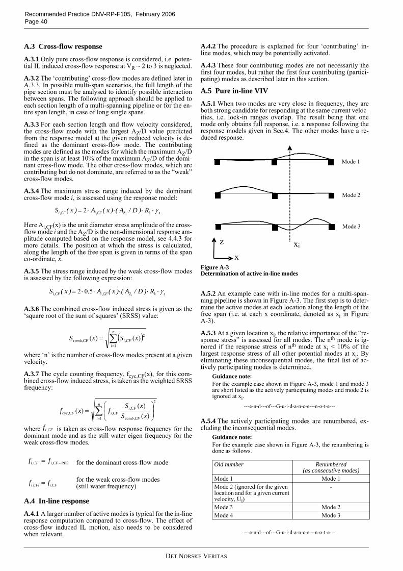
Recommended Practice DNV-RP-F105, February 2006 Page 40
A.3 Cross-flow response
A.3.1 Only pure cross-flow response is considered, i.e. poten-tial IL induced cross-flow response at VR ~ 2 to 3 is neglected.
A.3.2 The ‘contributing’ cross-flow modes are defined later inA.3.3. In possible multi-span scenarios, the full length of thepipe section must be analysed to identify possible interactionbetween spans. The following approach should be applied toeach section length of a multi-spanning pipeline or for the en-tire span length, in case of long single spans.
A.3.3 For each section length and flow velocity considered,the cross-flow mode with the largest AZ/D value predictedfrom the response model at the given reduced velocity is de-fined as the dominant cross-flow mode. The contributingmodes are defined as the modes for which the maximum AZ/Din the span is at least 10% of the maximum AZ/D of the domi-nant cross-flow mode. The other cross-flow modes, which arecontributing but do not dominate, are referred to as the “weak”cross-flow modes.
A.3.4 The maximum stress range induced by the dominantcross-flow mode i, is assessed using the response model:
Here Ai,CF(x) is the unit diameter stress amplitude of the cross-flow mode i and the AZ/D is the non-dimensional response am-plitude computed based on the response model, see 4.4.3 formore details. The position at which the stress is calculated,along the length of the free span is given in terms of the spanco-ordinate, x.
A.3.5 The stress range induced by the weak cross-flow modesis assessed by the following expression:
A.3.6 The combined cross-flow induced stress is given as the‘square root of the sum of squares’ (SRSS) value:
where ‘n’ is the number of cross-flow modes present at a givenvelocity.
A.3.7 The cycle counting frequency, fcyc,CF(x), for this com-bined cross-flow induced stress, is taken as the weighted SRSSfrequency:
where is taken as cross-flow response frequency for thedominant mode and as the still water eigen frequency for theweak cross-flow modes.
A.4 In-line response
A.4.1 A larger number of active modes is typical for the in-lineresponse computation compared to cross-flow. The effect ofcross-flow induced IL motion, also needs to be consideredwhen relevant.
A.4.2 The procedure is explained for four ‘contributing’ in-line modes, which may be potentially activated.
A.4.3 These four contributing modes are not necessarily thefirst four modes, but rather the first four contributing (partici-pating) modes as described later in this section.
A.5 Pure in-line VIV
A.5.1 When two modes are very close in frequency, they areboth strong candidate for responding at the same current veloc-ities, i.e. lock-in ranges overlap. The result being that onemode only obtains full response, i.e. a response following theresponse models given in Sec.4. The other modes have a re-duced response.
Figure A-3 Determination of active in-line modes
A.5.2 An example case with in-line modes for a multi-span-ning pipeline is shown in Figure A-3. The first step is to deter-mine the active modes at each location along the length of thefree span (i.e. at each x coordinate, denoted as xi in FigureA-3).
A.5.3 At a given location xi, the relative importance of the “re-sponse stress” is assessed for all modes. The nth mode is ig-nored if the response stress of nth mode at xi < 10% of thelargest response stress of all other potential modes at xi. Byeliminating these inconsequential modes, the final list of ac-tively participating modes is determined.
Guidance note:For the example case shown in Figure A-3, mode 1 and mode 3are short listed as the actively participating modes and mode 2 isignored at xi.
---e-n-d---of---G-u-i-d-a-n-c-e---n-o-t-e---
A.5.4 The actively participating modes are renumbered, ex-cluding the inconsequential modes.
Guidance note:For the example case shown in Figure A-3, the renumbering isdone as follows.
---e-n-d---of---G-u-i-d-a-n-c-e---n-o-t-e---
for the dominant cross-flow mode
for the weak cross-flow modes (still water frequency)
skZCF,iCF,i R)D/A()x(A)x(Si
γ⋅⋅⋅⋅= 2
skZCF,iCF,i R)D/A()x(A.)x(Si
γ⋅⋅⋅⋅⋅= 502
( )∑=
=n
iCFiCFcomb xSxS
1
2,, )()(
∑=
⎟⎟⎠
⎞⎜⎜⎝
⎛=
n
i CFcomb
CFiCFiCFcyc xS
xSfxf
1
2
,
,,, )(
)()(
CFif ,
RESCFiCFi ff −= ,,
CF,iCFi,i ff =
Old number Renumbered (as consecutive modes)
Mode 1 Mode 1Mode 2 (ignored for the given location and for a given current velocity, Ui)
-
Mode 3 Mode 2Mode 4 Mode 3
Mode 1
Mode 2
Mode 3
x
z xi
DET NORSKE VERITAS
Recommended Practice DNV-RP-F105, February 2006Page 41
A.5.5 Two adjacent modes can either compete with each other,when their frequencies are close or they can act as independentmodes, when their frequencies are widely separated.
A.5.6 For computational purposes, the renumbered mode sys-tem should be used, when two adjacent mode numbers need tobe checked.
A.5.7 Two adjacent modes are competing, if the ratio of theirfrequencies is lower than 2, i.e.
where fn is the eigen frequency of the nth mode number.
A.5.8 When the modes compete, only one of the modes is as-sumed to respond (i.e. is permitted to respond) with the full A/D as given in Sec.4. This mode is referred to as the dominantin-line mode. The remaining actively participating modes willbe subject to a reduction in the permissible amplitude and theresponse of these weak (non-dominant) in-line modes may bereduced by a factor of 0.5.
A.5.9 Every adjacent mode combination needs to be checked,to find out which ones will compete and which modes will winthe competition. This implies the following combinationsneeds to be checked:
— Mode 1 – Mode 2— Mode 2 – Mode 3— Mode 3 – Mode 4
A.5.10 Evaluate the stress at the given location xi, for all theactively participating modes. The competing mode reductionfactor, αj, is multiplied to the stresses associated with each ofthe mode shapes, based on the following rules:Non-competing mode combinations
— For non-competing mode combinations, the αj, is always1, i.e. there is no stress reduction.
Competing mode combinations
— The mode associated with the largest stress (i.e. dominantmode) within each competing mode combination gets anαj of 1.
— The weak mode within each competing mode combinationgets an αj of 0.5.
— The competing modes reduction factor, αj, should be mul-tiplied to the stresses, for each mode combination checked.This implies that for some mode numbers, it can be ap-plied more than once on the same mode number.
Guidance note:Consider an example case, where
— Mode 1 and Mode 2 are competing and assume Mode 1 isthe dominant mode in this competition. This implies Mode1 get an αj of 1 and Mode 2 gets an αj of 0.5.
— Mode 2 and Mode 3 are competing and assume Mode 2 isthe dominant mode in this competition. This implies Mode2 get an αj of 1 and Mode 3 gets an αj of 0.5.
— Mode 3 and Mode 4 are competing and assume Mode 4 isthe dominant mode in this competition. This implies Mode4 get an αj of 1 and Mode 3 gets an αj of 0.5.
This will effectively imply that:
— Mode 1 get an αj of 1 — Mode 2 gets an αj of 0.5— Mode 3 gets an αj of 0.25 (= 0.5 · 0.5)
— Mode 4 gets an αj of 1.0
Since Mode 3 is competing with Mode 2 as well as Mode 4, thisfurther reduction (0.25) is justified.
---e-n-d---of---G-u-i-d-a-n-c-e---n-o-t-e---
A.5.11 The pure in-line VIV stress range Sj,IL (x) is written as:
where the effect of the reduction factor for competing modes,αj, has been included. For more details, see Sec.4.3.3.
Guidance note:Applying no reduction factor for competing modes (αj = 1.0) isconservative.
---e-n-d---of---G-u-i-d-a-n-c-e---n-o-t-e---
A.6 Cross-flow induced in-line VIV
A.6.1 It is assumed that only the dominant cross-flow modecan potentially contribute to the cross-flow induced in-linemotion.
A.6.2 The in-line mode with its eigen frequency closest totwice the dominant cross-flow response frequency is chosen asthe candidate for the cross-flow induced in-line:
where j = 1,2,….,2n and i denotes the dominating cross-flowmode.
A.6.3 The in-line stress range corresponding to a figure 8 orhalf-moon motion, , i.e., the dominant cross-flow mode induces the jth in-line mode and the correspondingin-line stress can be written as:
A.6.4 The stress for the in-line mode that is potentially oscil-lated by cross-flow induced in-line motion, is taken as:
A.6.5 The combined in-line stress is given as the ‘square rootof the sum of squares’ (SRSS) value:
A.6.6 The cycle counting frequency for the in-line modes isbased on the following principles:
— for pure in-line modes, the cycle counting frequency is thestill water eigen frequency of the in-line mode
— for the cross-flow induced in-line mode, the cycle count-ing frequency is taken as twice the cross-flow responsefrequency of the dominant cross-flow mode, i.e. 2 · .
A.6.7 The combined stress and associated cycle counting fre-quency, using SRSS approach, is given by
21 <+
n
n
ff
γψα α ⋅⋅⋅⋅⋅= ILYILjjILj DAxAxS ,,, )/()(2)(
( )RESCFiILj ff −⋅− ,, 2min
)(, xS jDOMCFIL −−
γ⋅⋅⋅⋅⋅=− kZILjCFILj RDAxAxSDOM
)/()(4.02)( ,,
( ))(,)(max)( ,,, xSxSxS CFILjILjILj −=
( )∑=
=n
jILjILcomb xSxS
2
1
2,, )()(
RESCFif −,
∑=
⎟⎟⎠
⎞⎜⎜⎝
⎛=
n
j ILcomb
ILjILjILcyc xS
xSfxf
2
1
2
,
,,, )(
)()(
DET NORSKE VERITAS
Recommended Practice DNV-RP-F105, February 2006 Page 42
APPENDIX B VIV MITIGATION
B.1 VIV mitigation methods
B.1.1 The most commonly used vortex suppression devicesare helical strakes. Their function is to trigger separation in or-der to decrease the vortex shedding correlation along the riser.They increase the cost of the pipeline, and they will complicatehandling during installation. The in-line drag coefficient is in-creased by introducing strakes.
B.1.2 The important parameters for the strake design are theheight and pitch of the helical strakes for a given pipeline di-ameter. The overall performance characteristics of a givenstrake design will vary with the current velocities.
B.1.3 The effectiveness of VIV suppression devices, such asVIV strakes needs to be qualified. It is recommended that anindependent verification of the effectiveness of VIV suppres-sion devices is performed by a competent verification body.
B.1.4 Qualification process will typically include the follow-ing, for a given strake design:
— model test results with and without strakes— effect of hydrodynamic scaling— range of current velocities and associated efficiency— durability and impact assessments— effect of marine growth— effect of surface finish.
B.1.5 More detailed information is given in DNV-RP-F204with respect to qualification of VIV strakes.
B.2 Span rectification methods
B.2.1 Reference is made to Sec.9 of DNV-OS-F101 for spanrectification procedures and methods.
B.2.2 Survey, follow-up and documentation requirementsshould follow the principles given in Sec.9 of DNV-OS-F101.
DET NORSKE VERITAS
Recommended Practice DNV-RP-F105, February 2006Page 43
APPENDIX C VIV IN OTHER OFFSHORE APPLICATIONS
C.1 Main application scope
C.1.1 The primary focus and the main application scope of thisRP is free spanning subsea pipelines as described in Sec.1.3.
C.1.2 The fundamental principles given in this RP may also beapplied and extended to other offshore elements such as cylin-drical structural elements of the jackets, risers from fixed plat-forms etc., at the designer’s discretion. The limitations thatapply are discussed in this section.
C.2 Riser VIV
C.2.1 Important differences with respect to the riser VIV, ascompared to free spanning VIV are listed below:
— The circular particle flow due to waves.— Risers will not experience the uniform currents over the
span, as assumed in free span assessments.— Typically for long risers, the higher order modes are excit-
ed. — For long span lengths and/or when the flow is sheared,
several modes may be excited simultaneously. For suchrisers the tension will vary, and the response is dominatedby loading (power input) in some parts of the riser whileother parts are contributing to the damping of the system(power output). In such cases DNV-RP-F105 is not appli-cable.
C.2.2 For short riser span lengths, typical for steel risers sup-ported by a jacket structure and when the current is uniform,the response models given in Sec.4 of this RP (DNV-RP-F105)can be applied. For short risers the lowest eigen modes are typ-ically excited. In such cases DNV-RP-F105 will predict bothin-line and cross-flow VIV provided that the natural frequen-cies are calculated based on relevant boundary conditions.
C.2.3 If no onset of VIV is allowed, the screening criterionmay be applied.
C.2.4 Other subsea cylindrical structural components (e.g.braces, trusses, etc.) can also be evaluated, using this RP at thedesigners discretion and judgement. The following conditionsshould however, be carefully evaluated:
— uniform current assumption— frequencies and mode shapes should be based on detailed
FE analysis— L/D ratio should be within the RP’s design range— location of the structural element (relevance of Wave-in-
duced VIV, which is not covered by this RP).
C.2.5 For a detailed account of riser VIV and applicable meth-odologies, reference is made to the DNV-RP-F204 “Riser Fa-tigue”.
DET NORSKE VERITAS
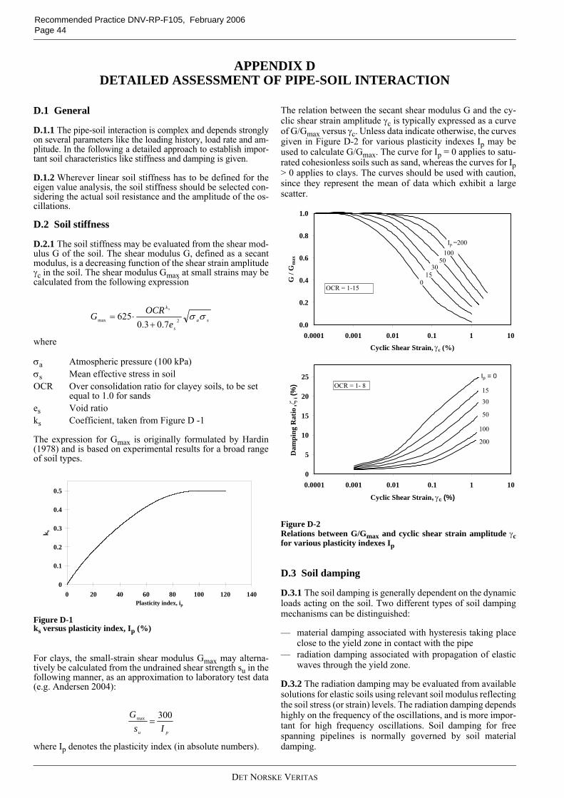
Recommended Practice DNV-RP-F105, February 2006 Page 44
APPENDIX D DETAILED ASSESSMENT OF PIPE-SOIL INTERACTION
D.1 General
D.1.1 The pipe-soil interaction is complex and depends stronglyon several parameters like the loading history, load rate and am-plitude. In the following a detailed approach to establish impor-tant soil characteristics like stiffness and damping is given.
D.1.2 Wherever linear soil stiffness has to be defined for theeigen value analysis, the soil stiffness should be selected con-sidering the actual soil resistance and the amplitude of the os-cillations.
D.2 Soil stiffness
D.2.1 The soil stiffness may be evaluated from the shear mod-ulus G of the soil. The shear modulus G, defined as a secantmodulus, is a decreasing function of the shear strain amplitudeγc in the soil. The shear modulus Gmax at small strains may becalculated from the following expression
where
The expression for Gmax is originally formulated by Hardin(1978) and is based on experimental results for a broad rangeof soil types.
Figure D-1 ks versus plasticity index, Ip (%)
For clays, the small-strain shear modulus Gmax may alterna-tively be calculated from the undrained shear strength su in thefollowing manner, as an approximation to laboratory test data(e.g. Andersen 2004):
where Ip denotes the plasticity index (in absolute numbers).
The relation between the secant shear modulus G and the cy-clic shear strain amplitude γc is typically expressed as a curveof G/Gmax versus γc. Unless data indicate otherwise, the curvesgiven in Figure D-2 for various plasticity indexes Ip may beused to calculate G/Gmax. The curve for Ip = 0 applies to satu-rated cohesionless soils such as sand, whereas the curves for Ip> 0 applies to clays. The curves should be used with caution,since they represent the mean of data which exhibit a largescatter.
Figure D-2 Relations between G/Gmax and cyclic shear strain amplitude γcfor various plasticity indexes Ip
D.3 Soil damping
D.3.1 The soil damping is generally dependent on the dynamicloads acting on the soil. Two different types of soil dampingmechanisms can be distinguished:
— material damping associated with hysteresis taking placeclose to the yield zone in contact with the pipe
— radiation damping associated with propagation of elasticwaves through the yield zone.
D.3.2 The radiation damping may be evaluated from availablesolutions for elastic soils using relevant soil modulus reflectingthe soil stress (or strain) levels. The radiation damping dependshighly on the frequency of the oscillations, and is more impor-tant for high frequency oscillations. Soil damping for freespanning pipelines is normally governed by soil materialdamping.
σa Atmospheric pressure (100 kPa)σs Mean effective stress in soilOCR Over consolidation ratio for clayey soils, to be set
equal to 1.0 for sandses Void ratioks Coefficient, taken from Figure D -1
sa
s
k
eOCRG
s
σσ2max 7.03.0625
+⋅=
0
0.1
0.2
0.3
0.4
0.5
0 20 40 60 80 100 120 140Plasticity index, ip
k s
pu IsG 300max =
γ
0.0
0.2
0.4
0.6
0.8
1.0
0.0001 0.001 0.01 0.1 1 10
Cyclic Shear Strain, c (%)
G /
Gm
axOCR = 1-15
Ip =2000100
5030
150
0
5
10
15
20
25
0.0001 0.001 0.01 0.1 1 10
Cyclic Shear Strain, c (%)
Dam
ping
Rat
io,
i (%
) OCR = 1- 8
100
50
30
15
Ip = 0
ζ
γ
200
DET NORSKE VERITAS
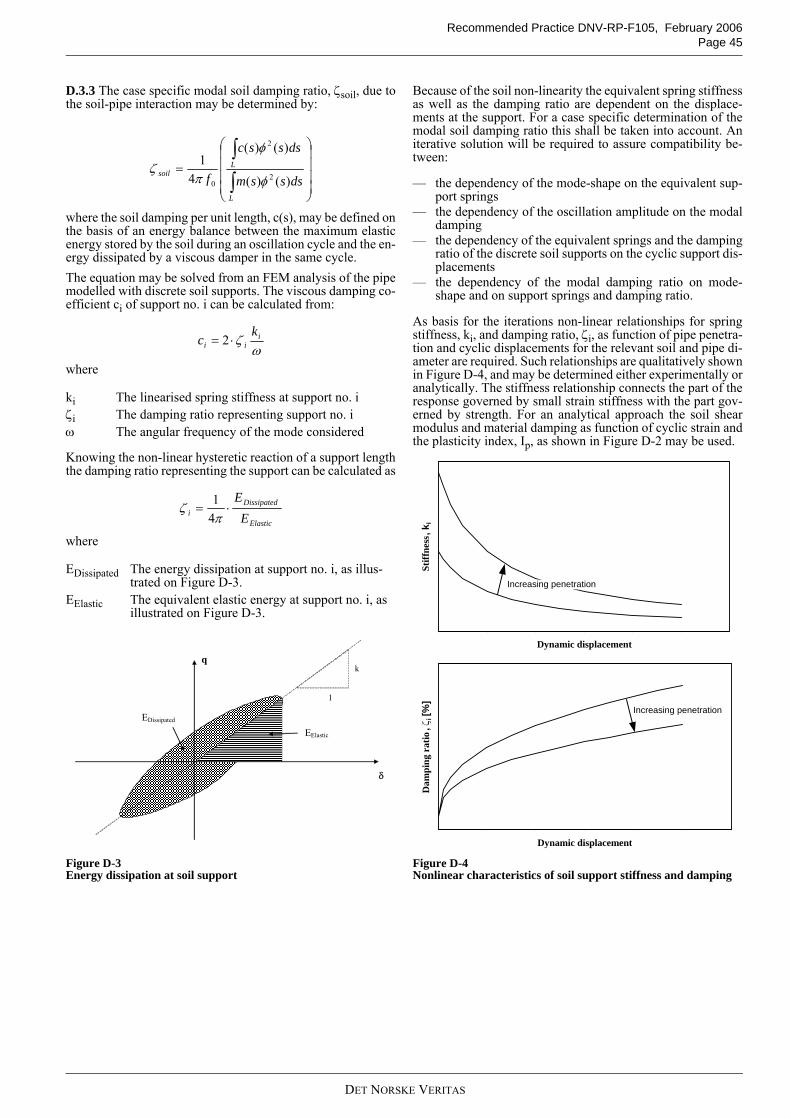
Recommended Practice DNV-RP-F105, February 2006Page 45
D.3.3 The case specific modal soil damping ratio, ζsoil, due tothe soil-pipe interaction may be determined by:
where the soil damping per unit length, c(s), may be defined onthe basis of an energy balance between the maximum elasticenergy stored by the soil during an oscillation cycle and the en-ergy dissipated by a viscous damper in the same cycle. The equation may be solved from an FEM analysis of the pipemodelled with discrete soil supports. The viscous damping co-efficient ci of support no. i can be calculated from:
where
Knowing the non-linear hysteretic reaction of a support lengththe damping ratio representing the support can be calculated as
where
Figure D-3 Energy dissipation at soil support
Because of the soil non-linearity the equivalent spring stiffnessas well as the damping ratio are dependent on the displace-ments at the support. For a case specific determination of themodal soil damping ratio this shall be taken into account. Aniterative solution will be required to assure compatibility be-tween:
— the dependency of the mode-shape on the equivalent sup-port springs
— the dependency of the oscillation amplitude on the modaldamping
— the dependency of the equivalent springs and the dampingratio of the discrete soil supports on the cyclic support dis-placements
— the dependency of the modal damping ratio on mode-shape and on support springs and damping ratio.
As basis for the iterations non-linear relationships for springstiffness, ki, and damping ratio, ζi, as function of pipe penetra-tion and cyclic displacements for the relevant soil and pipe di-ameter are required. Such relationships are qualitatively shownin Figure D-4, and may be determined either experimentally oranalytically. The stiffness relationship connects the part of theresponse governed by small strain stiffness with the part gov-erned by strength. For an analytical approach the soil shearmodulus and material damping as function of cyclic strain andthe plasticity index, Ip, as shown in Figure D-2 may be used.
Figure D-4 Nonlinear characteristics of soil support stiffness and damping
ki The linearised spring stiffness at support no. iζi The damping ratio representing support no. iω The angular frequency of the mode considered
EDissipated The energy dissipation at support no. i, as illus-trated on Figure D-3.
EElastic The equivalent elastic energy at support no. i, as illustrated on Figure D-3.
⎟⎟⎟⎟
⎠
⎞
⎜⎜⎜⎜
⎝
⎛
=∫
∫
L
Lsoil
dsssm
dsssc
f )()(
)()(
41
2
2
0 φ
φ
πζ
ωζ i
iik
c ⋅= 2
Elastic
Dissipatedi E
E⋅=
πζ
41
EDissipated
EElastic
k
1
δ
q
0
0.2
0.4
0.6
0.8
1
1.2
1.4
1.6
0 0.002 0.004 0.006 0.008 0.01 0.012
Dynamic displacement
Stiff
ness
, ki
0
5
10
15
20
25
30
35
40
0 0.002 0.004 0.006 0.008 0.01 0.012
Dynamic displacement
Dam
ping
rat
io,ζ
i [%
]
Increasing penetration
Increasing penetration
DET NORSKE VERITAS

Recommended Practice DNV-RP-F105, February 2006 Page 46
DET NORSKE VERITAS