Spectral Analysis of Nonstationary Spacecraft Vibration Data

Nonstationary Signal Tutorial(release beta 0.1)
Jon Claerbout with Kaiwen Wang
Stanford University
c� April 5, 2018


Contents
0.1 PREFACE . . . . . . . . . . . . . . . . . . . . . . . . . . . . . . . . . . . . i
0.2 INTRODUCTION . . . . . . . . . . . . . . . . . . . . . . . . . . . . . . . . ii
0.2.1 What can you do with this stu↵? . . . . . . . . . . . . . . . . . . . . ii
0.3 PREDICTION ERROR FILTER == PEF . . . . . . . . . . . . . . . . . . iii
0.3.1 PEF history . . . . . . . . . . . . . . . . . . . . . . . . . . . . . . . . iii
0.3.2 PEFs present and future . . . . . . . . . . . . . . . . . . . . . . . . . iii
0.4 CREDITS AND THANKS . . . . . . . . . . . . . . . . . . . . . . . . . . . iv
1 Nonstationary scalar signals 1
1.0.1 Why should residuals be IID? . . . . . . . . . . . . . . . . . . . . . . 1
1.0.2 Prediction-error filtering (deconvolution) . . . . . . . . . . . . . . . . 1
1.1 THE HEART OF NONSTATIONARY PEF WITH NO CALCULUS . . . . 2
1.1.1 Code for prediction error = deconvolution = autoregression . . . . . 3
1.1.2 The outside world—real estate . . . . . . . . . . . . . . . . . . . . . 4
1.1.3 Why does the residual into the adjoint give the gradient? . . . . . . 4
1.1.4 Hyperbolic penalty function . . . . . . . . . . . . . . . . . . . . . . . 5
1.2 ESTIMATING TOGETHER MISSING DATA WITH ITS PEF . . . . . . . 6
1.2.1 Old 1-D examples I have done in the stationary world . . . . . . . . 7
1.2.2 Epsilon . . . . . . . . . . . . . . . . . . . . . . . . . . . . . . . . . . 7
1.2.3 Safely using a time-variable epsilon . . . . . . . . . . . . . . . . . . . 9
1.2.4 How can the nonstationary PEF operator be linear? . . . . . . . . . 9
1.2.5 Diverse applications . . . . . . . . . . . . . . . . . . . . . . . . . . . 9
1.2.6 My favorite wavelet for modelers . . . . . . . . . . . . . . . . . . . . 11
1.2.7 Sparse decon results that I aspire to reconquer . . . . . . . . . . . . 11

CONTENTS
2 Spatial deconvolution 15
2.1 TIME AND SPACE . . . . . . . . . . . . . . . . . . . . . . . . . . . . . . . 15
2.1.1 Bubble removal . . . . . . . . . . . . . . . . . . . . . . . . . . . . . . 16
2.1.2 Two-dimensional PEF . . . . . . . . . . . . . . . . . . . . . . . . . . 17
2.1.3 2-D PEFs as plane wave destructors and plane wave builders . . . . 18
2.1.4 Example of a 2-D PEF applied to a seismic section . . . . . . . . . . 19
2.1.5 Stretch matching . . . . . . . . . . . . . . . . . . . . . . . . . . . . . 19
2.2 DISJOINT REGIONS OF SPACE . . . . . . . . . . . . . . . . . . . . . . . 20
2.2.1 Geostatistics . . . . . . . . . . . . . . . . . . . . . . . . . . . . . . . 20
2.2.2 Gap filling . . . . . . . . . . . . . . . . . . . . . . . . . . . . . . . . . 21
2.2.3 Rapid recognition of a spectral change . . . . . . . . . . . . . . . . . 22
2.2.4 Boundaries between regions of constant spectrum . . . . . . . . . . . 22
2.2.5 What physical phenomena gives the spectra of a 3-D PEF? . . . . . 24
3 Vector-valued signals 25
3.0.6 Multi channels == vector-valued signals . . . . . . . . . . . . . . . . 25
3.1 MULTIDIMENSIONAL PEF . . . . . . . . . . . . . . . . . . . . . . . . . . 27
3.1.1 Vector signal scaling . . . . . . . . . . . . . . . . . . . . . . . . . . . 27
3.1.2 Pseudocode for vector signals . . . . . . . . . . . . . . . . . . . . . . 28
3.1.3 How the conjugate gradient method came to be oversold . . . . . . . 29
3.1.4 The PEF output is orthogonal to its inputs . . . . . . . . . . . . . . 29
3.1.5 Restoring source spectra . . . . . . . . . . . . . . . . . . . . . . . . . 29
3.2 CHOLESKY DECORRELATING AND SCALING . . . . . . . . . . . . . . 30
3.3 ROTATING FOR SPARSITY . . . . . . . . . . . . . . . . . . . . . . . . . . 31
3.3.1 Finding the angle of maximum sparsity (minimum entropy) . . . . . 31
3.3.2 3-component vector data . . . . . . . . . . . . . . . . . . . . . . . . 32
3.3.3 Channel order and polarity . . . . . . . . . . . . . . . . . . . . . . . 32
3.4 RESULTS OF KAIWEN WANG . . . . . . . . . . . . . . . . . . . . . . . . 33
4 Fitting while whitening residuals 37
4.1 UPDATING MODELS WHILE UPDATING THE PEF . . . . . . . . . . . 37
4.1.1 Applying the adjoint of a streaming filter . . . . . . . . . . . . . . . 38
4.1.2 Code for applying A⇤A while estimating A . . . . . . . . . . . . . . 38

CONTENTS
4.1.3 Streaming . . . . . . . . . . . . . . . . . . . . . . . . . . . . . . . . . 38
4.2 REGRIDDING: INVERSE INTERPOLATION OF SIGNALS . . . . . . . . 39
4.2.1 Sprinkled signals go to a uniform grid via PEFed residuals . . . . . . 40
4.2.2 Is the theory worthwhile? . . . . . . . . . . . . . . . . . . . . . . . . 42
4.2.3 Repairing the navigation . . . . . . . . . . . . . . . . . . . . . . . . . 43
4.2.4 Daydreams . . . . . . . . . . . . . . . . . . . . . . . . . . . . . . . . 43
5 Appendices 45
5.1 WHY PEFs HAVE WHITE OUTPUT . . . . . . . . . . . . . . . . . . . . . 45
5.1.1 Why 1-D PEFs have white output . . . . . . . . . . . . . . . . . . . 45
5.1.2 Why 2-D PEFs have white output . . . . . . . . . . . . . . . . . . . 46
5.2 THE HEART OF NONSTATIONARY PEF USING CALCULUS . . . . . . 47

CONTENTS

Front matter
The perfect is the enemy of the good.
0.1 PREFACE
Sixty years ago an 80 year old mathematician put out a book, “The elliptic functions asthey should be.” I put this booklet out at my 80th birthday too. I might feel the way themathematician did, but I have a di↵erent story for you.
After what in 2014 was to be my final book, Geophysical Image Estimation by Example(GIEE), I stumbled on an approach to a large amount of geophysical data model fitting thatis much simpler than traditional approaches. Even better, it avoids the often unreasonableacademic presumption of stationarity (i.e., time and space invariant statistics). Not onlythat, but, as I was finishing GIEE, I was horrified to realize that I had invested much inmanaging scalar data on an irregular grid, but the method did not scale well to signal data.Altogether, I could not resist embarking on this booklet.
Any participant is welcome to contribute illustrations (and ideas)—perhaps becoming acoauthor, even eventually taking over this manuscript. The first need now is more examples.Ultimately, all the examples should be presented in reader rebuildable form.
My previous book GIEE is freely available at http://sep.stanford.edu/sep/prof/or in paper for a small price at many booksellers, or at the printer, Lulu.com. It is widelyreferenced herein.
Early beta versions of this booklet will fail to provide rebuildable illustrations. I am nolonger coding myself, so if there are ever to be rebuildable illustrations, I need coauthors.I set for myself the goal to take this booklet out out of beta when 50% of the illustrationscan be destroyed and rebuilt by readers.
The most recent version of this manuscript should be at the website Jon Claerbout’sclassroom. Check here: http://sep.stanford.edu/sep/prof/. The manuscript you arenow reading was formed April 5, 2018.
i
ii CONTENTS
0.2 INTRODUCTION
Nonstationary data is data with statistics that vary with time or space. Concepts here areilluminated with pseudo code, with modeled data, and with real data.
0.2.1 What can you do with this stu↵?
1. Build models to fit data with nonstationary statistics.
2. Perform blind deconvolution (estimate and remove a source wavelet).
3. Fill data gaps. Interpolate beyond aliasing (sometimes).
4. Transform residuals to IID (Independent, Identically Distributed) while fitting.
5. Swap easily among `1, `2, hyperbolic, and inequality penalties.
6. Stretch a signal unevenly to match another. Images too.
7. Predict price based on diverse aspects.
8. Remove crosstalk in multichannel signals (vector data).
9. Model robustly (i.e., multivariate median versus the mean).
10. Shave models with Occam’s razor outdoing the `1 norm.
11. Bring randomly positioned data to a uniform Cartesian grid.
12. Join the world of BIG DATA by grasping multiple aspects of back projection.
This booklet is novel by attacking data what is nonstationary, meaning that its statisticalcharacterization is not constant in time and space. This approach works by including a newdata value to a previously solved imaging problem. The newly arrived data value requiresus to make a small adjustment to the solution. Then we continue with all the other datavalues.
Although we begin here narrowly with a single 1-D scalar signal yt, we soon expandbroadly with yt(x, y, z) representing multidimensional data (images and voxels) and thenmulticomponent (vector-valued) signals ~yt.
Many researchers dealing with physical continua use “inverse theory” with little graspof how to supply the “inverse covariance matrix.” The needed algorithms including pseudocode are here.
Most of the time-series literature presumes data spectra are time invariant (stationary),while most applications involve spectra that change in time and space. Therefore, thereis a real need for nonstationary tools. These capabilities are particularly important inhigher dimensional problems, slightly in time, and more strongly in space. A basic problemin Geophysics is the lack of adequately dense data sampling in space, and wide-spreadnonstationarity (especially in space). Such undersampling and nonstationarity arises bothfor statistical reasons, as well as physical reasons such as location versus angle.

0.3. PREDICTION ERROR FILTER == PEF iii
0.3 PREDICTION ERROR FILTER == PEF
Knowledge of an autocorrelation is equivalent to knowledge of a spectrum. Less well knownis that both are equivalent to knowledge of a Prediction Error Filter (PEF). PEFs sharemany properties with di↵erential equations. A PEF is like a di↵erential equation thatwhen driven by a random noise source, it produces data with the spectrum of interest. Byspectrum, I mean not only the temporal spectrum, but also 3-D spatial spectra. The PEFis commonly estimated from data by least squares procedures that we soon see.
0.3.1 PEF history
The name “Prediction Error Filter” appears first in the petroleum exploration industryalthough the idea emerges initially in the British market forecasting industry in the 1920sas the Yule-Walker equations (a.k.a. autoregression). The same equations next appear in1949 in a book by Norbert Wiener in an appendix by Norman Levinson. Soon after, EndersRobinson extended the PEF idea to multichannel (vector-valued) signals. Meanwhile, as thepetroleum exploration industry became computerized it found a physical model for scalar-valued PEFs. They found a lot of oil with it; and they pursued PEFs vigorously until about1970 when their main focus shifted (to where it remains today) to image estimation. Myfriends John Burg and John Sherwood understood a 2-D extension to the PEF idea butit went unused until I discovered the helix interpretation of it (in about 1998) and used itextensively in my 2014 book Geophysical Image Estimation by Example (GIEE). Beyond2-D, the PEF idea naturally extends to any number of dimensions. (Exploration industrydata exists in a 5-D space, time plus two Earth surface geographical coordinates for eachenergy source plus another two for each signal receiver.) I expected the study of submarinewarfare to result in conceptual advances with acoustic antennas; etc, but, I am not awareof whatever fundamentals it may have uncovered.
0.3.2 PEFs present and future
From an application perspective the weakness of autocorrelation, spectrum, and classic PEFis the lack of a natural extension to nonstationarity. Like autocorrelation and spectrum, thePEF theory became clumsy when applied to real-world data in which the statistics variedwith time and space. Since my 2014 book, Sergey Fomel and I have found a way to extendthe PEF concept to nonstationary data. Not only have we discovered an extension, it isalso easier to understand and to code! This ease promises quick results and, it looks likefun! Although I recently turned 80, I cannot stop thinking about it.
In addition to all the old-time activities that are beginning to get easier and better,we can speculate it is going to be fun for even more reasons. The nonstationary PEFsin this document bring us many flavors of back projection. They share that aspect withthe emerging field of machine learning. Who is going to have more fun, them or us? Weare quite model-based; therefore, we should have the advantage of needing less data tofind robust methods and more reliable results. Never-the-less, they bring a young, rapidly-growing, energetic community to the table, and that is another reason we are going to havefun.

iv CONTENTS
Beyond introduction to nonstationary PEFs, find in this booklet a surprising new con-cept promising a new direction. Quantum theory associates momentum with Fourier spaceleading to the uncertainty principle that says they cannot simultaneously know position andvelocity. Although we are not doing quantum mechanics, we too often feel such mathemati-cal constraints in our work. PEFs like di↵erential equations and finite-di↵erence equations,often have coe�cients that change abruptly compared to wavelengths emitted. There iswhere the character of a signal changes abruptly. With an image of a person—even a blackand white image—the spatial spectrum changes abruptly at the transition from from skinto hair. Also in this document is a strategy for recognition of such a sharp boundary alongwith the PEFs that pertain to each side of the boundary.
0.4 CREDITS AND THANKS
Sergey Fomel triggered this direction of research when he solved the nonstationarity problemthat I had posed but could not solve. Bob Clapp ran an inspiring summer research group.Stewart Levin generously welcomes my incomplete thoughts on many topics. He page editedand provided a vastly cleaner 1-D whiteness proof. John Burg set me on the track forunderstanding the 2-D PEF. Kaiwen Wang worked with me and made all the illustrationsin the multichannel chapter. Joseph Jennings provided the field-data debubble example andcommented on early versions of the multichannel chapter. Jason Chang assisted me withLaTeX. Anne Cain did page editing.
Finally, my unbounded gratitude goes to my beloved wife Diane, who accepted to livewith a kind of an alien. Without her continuous love and support over half a century, noneof my books could have existed.

Chapter 1
Nonstationary scalar signals
While working to fit a model to observed data, the misfit should be managed by a prin-ciple from field of Statistics. We should arrange those statistics to be Independent andIdentically Distributed (IID). In practice, the “ID” means gain should be chosen to giveresiduals a generally uniform variance over physical space; it is simply a matter of scaling.The remaining “I” in IID means “independent,” our topic here. Autocorrelations shouldtend to impulses, meaning spectra should tend to whiteness (uniform variance) which isaccomplished herein with Prediction-Error Filters (PEFs) soon to be defined.
1.0.1 Why should residuals be IID?
With least squares fitting modeled data to observed data, small residuals are squared; sothey tend to be ignored. Thus, the entire physical space and Fourier space of residualsshould be scaled up to easily visible levels to ensure all aspects of the data have beenprobed. The statistical principle that model fitting residuals should be IID says almostevery image estimation situation calls for using PEFs. They are introduced next.
1.0.2 Prediction-error filtering (deconvolution)
A widespread generic model for signal and image data is that the data originated fromindependent causes that were somehow smoothed, filtered, or convolved before reaching usas data. Because the PEF returns us to uncorrelated and apparently independent sources, itis said to be “deconvolved.” Those uncorrelated sources will tend to contain all frequenciesin a generally uniform amount.
Start with a channel of data (a signal of many thousands of values). We denote thesedata numbers by y = (y0, y1, y2, · · ·). A little patch of numbers that we call a “filter” isdenoted by a = (a0, a1, a2, · · · , an⌧ ). In pseudo code these filter numbers are denoted bya(0), a(1),...,a(ntau). Likewise code for the data. The filter numbers slide across thedata numbers with the leader being a(0). An equation for sliding the filter numbers acrossthe data numbers obtaining the output rt is rt =
Pn⌧⌧=0 a⌧yt�⌧ . In a stationary world, the
filter values are constants. In our nonstationary world, the filter values change a tiny bitafter the arrival of each new data value.
1

2 CHAPTER 1. NONSTATIONARY SCALAR SIGNALS
Several computer languages allow the calculation x x + y to be represented by x+=y.We use this notation herein, likewise x-=y for subtraction. Pseudo code for finding r(t) is:
# CODE = CONVOLUTIONr(....) = 0.for all t {
do tau = 0, ntaur(t) += a(tau) * y(t-tau)
}
With each step in time we prepare to change the filter a(tau) a tiny bit. To specify thechange, we need a goal for the filter outputs r(t) to have minimum energy. To prevent thefilter a from becoming all zeros, we constrain the first filter coe�cient to be unity.
a = [ 1, a1, a2, a3, · · ·] (1.1)
To contend with the initial unit “1.0” outputting an input data value, the remaining filtercoe�cients try to destroy that data value. They must attempt to predict the input value’snegative. The filter output rt is the residual of the attempted prediction. The name of thefilter itself is the Prediction-Error Filter (PEF). PEFs are slightly misnamed because theirprediction portion predicts the data negative.
Intuitively, PEF output has sucked all the predictability from its input. Appendix 5.1.1Why 1-D PEFs have white output shows the PEF output tends to be spectrally white—tobe a uniform function of frequency. The longer the filter, the whiter the output. The namedeconvolution came about from a hypothetical model that the original sources were randomimpulses, but the received signal became spectrally colored (convolved) by reasons such aswave propagation. Thus, a PEF should return the data to its original state. It cannot restoreany delays—because the PEF is causal, meaning it has only knowledge of the past; therefore[· · · , a�2, a�1] = 0. P.E. filtering is sometimes called blind deconvolution—stressing thata is estimated as well as applied.
For now yt and a⌧ are scalar time functions at a point in space. Before we finish, theywill become time functions in an N -dimensional physical space like the four componentarray yt(x, y, z). Beyond that we will revert to a point in space, but extend to a vector-valued signal. Theory proceeds somewhat like with scalar signals, but data and predictionerror are vector functions like ~rt = (ut, vt, wt), where the PEF begins not with a 1.0 butwith a three component identity matrix I.
1.1 THE HEART OF NONSTATIONARY PEF WITH NO CALCULUS
At any one moment in time, we may think of the PEF outputP
⌧ a⌧yt�⌧ , as a dot productof the filter a onto some backwards piece of input data. Denote that backwards piece byd. (Other moments in time have other values in the d vector.) At that moment, the PEFoutput is a · d. Consider the exploratory filter a � ✏d, where ✏ is a tiny positive number.Its output rt is (a � ✏d) · d = (a · d) � ✏ (d · d). To reduce the size |rt| of the new outputresidual, these two terms must have opposite polarity; but rt = (a · d) may have eitherpolarity. Try instead the filter update (a � ✏ rtd). Its output is (a · d) � ✏ rt(d · d), which
Evolving document. Save the link, not the PDF. April 5, 2018

1.1. THE HEART OF NONSTATIONARY PEF WITH NO CALCULUS 3
on rearrangement is (a · d)(1� ✏ (d · d)), is easily assured smaller than rt = (a · d). Thus,
�a = � ✏ rt d = � ✏ rt yt�⌧ (1.2)
In summary:
Filter Definition Outputrt =
P⌧ a⌧yt�⌧
a = a⌧ d = yt�⌧ rt = a · da� ✏d First trial a · d� ✏ (d · d)
a� ✏ rt d Revision a · d� ✏ rt (d · d)a + �a Success! (a · d)(1� ✏ (d · d))
The last line says the filter change reduces the size of the residual rt = (a·d). Our numericalchoice of ✏ balances fitting the present versus fitting the past.
We arrived at Equation (1.2) by guesswork and logic, no calculus. Appendix 5.2 Theheart of nonstationary PEF using calculus derives the same result with two pages of cal-culus, but it does so under the limitation of the `2 norm. You might notice that rt andeach component of d in the expression ✏rtd can be stretched or shrunken by any polaritypreserving function, such as r r/|r|. After we finish with the basics, we will returnto specialized applications that take advantage of this extra flexibility. Hint: We will gobeyond `1.
1.1.1 Code for prediction error = deconvolution = autoregression
The following code does “deconvolution,” also known as “autoregression.”
r(...) = 0. # CODE = NONSTATIONARY PREDICTION ERRORa(...) = 0.a( 0 ) = 1.0do over time t { # r(t) = nonstationary prediction error.
do tau= 0, ntauda(tau) = 0r(t) += a(tau) * y(t-tau) # forward
do tau= 0, ntauda(tau) += r(t) * y(t-tau) # adjoint
da(0) = 0. # constraintdo tau= 0, ntau
a(tau) -= da(tau) * epsilon}
The #forward line in the code preceeding applies the filter to get the residual. The #adjointline in the code is building Equation (1.2). The adjoint operation is also called back-projection. The code preceeding, based on little more than the definition of dot product, isa example of a deeper principle in classroom mathematics. The line #forward is a matrixtimes a vector. The line #adjoint is also a matrix times a vector. It is the same matrixy(t-tau), but one tau loop does the matrix transpose of the other because one carriestau space to t space, while the other carries t space to tau space. The transpose of anymatrix is M⇤
ij = Mji. The line da(0)=0 is a constraint to prevent changing the a(0)=1maintaining the definition of r(t) as a residual. Common sense has given us the aboveexample of classroom fundamentals: Put the residual into the adjoint (transpose) to get the
Evolving document. Save the link, not the PDF. April 5, 2018

4 CHAPTER 1. NONSTATIONARY SCALAR SIGNALS
gradient; then go down. We got the gradient without ever calculating a derivative, withoutneeding a function to take the derivative of! If coding adjoints is new to you, I recommendChapter 1 in GIEE (Claerbout, 2014). It is free on the internet.
Suppose while running along time t, we find the line in the code above computing�a saying for practical purposes da(tau)=r(t)*y(t-tau) vanishes for all tau>0. Thisstatement would delight any stationary theorist, because the gradient vanishing �a = 0says we are finished. It is saying the residual r = rt is orthogonal to all the fitting functionsy⌧ = yt�⌧ . (A particular fitting function is y9 = yt�9.) With our nonstationary technology,we do not expect �a ever to be exactly zero, but we do expect it to get small and thenbounce around. The fluctuation in size of |�a| is not simply epsilon, but the fluctuationsdiminish as the residual becomes more and more orthogonal to all the fitting functions. Weare too new at this game to know precisely how to choose ✏, how much bouncing around toexpect, or how to characterize nonstationarity; but, we will come up with a good startingguess for ✏. While theorizing, there is much we will learn by experience.
1.1.2 The outside world—real estate
The regression updating approach introduced here is not limited to convolutional matrices.It applies to all regression equations. For each new regression row, subtract from the solutiona tiny suitably scaled copy of the new row. Move along; keep doing it. When you run out ofequations, you can recycle the old ones. By cycling around a vast number of times with anepsilon tending to zero, you converge to the stationary solution. This updating procedureshould be some long-known principle in mathematics. I have stumbled upon somethingcalled the Widrow-Ho↵ learning rule, which feels just like this updating.
For example, imagine a stack of records of home sales. The i-th member of the stack islike the t-th time of a signal. The first column contains the recorded sales prices. The nextcolumn contains the square footages, the third column contains the number of bathrooms,etc. Because many of these variables have all positive elements, we should allow for removingtheir collective means by including a column of all “ones.” In the signal application, thei-th column contains the signal at the i-th lag. Columns containing all positive numbersmight be replaced by their logarithms. The previously shown code finds ai coe�cients topredict (negatively) the signal. Associating lags with real-estate aspects, the code wouldpredict (the negative and possibly the logarithm of) the sales price. You have made thefirst step towards a learning machine.
1.1.3 Why does the residual into the adjoint give the gradient?
Basic geophysical model m estimation is summarized by the residual minimization 0 ⇡r(m) = Fm � d. In the special case in which F is a convolution matrix (downshiftedcolumns of data d), this formulation fits the estimation of a prediction filter m. But, formany applications we want a prediction-error filter a. Thus, we think of PEF estimationas the constraint a0 = 1 along with the augmented matrix Y = [d|F] where Y is also aconvolution matrix.
This tutorial document shows six codes for diverse applications of PEFs; therefore letus be sure that everyone is onboard with the idea that the gradient is a residual dumped
Evolving document. Save the link, not the PDF. April 5, 2018

1.1. THE HEART OF NONSTATIONARY PEF WITH NO CALCULUS 5
into a transposed modeling operator. Chapter 2 of my textbook GIEE (Claerbout, 2014)guides you through every step with a 2 ⇥ 3 matrix. In summary, the quadratic form youare minimizing is r · r = (m⇤F⇤ � d⇤)(Fm � d) with derivative by m⇤ being �m = F⇤r.Likewise, the derivative of a⇤Y⇤Ya by a⇤ is �a = Y⇤r.
1.1.4 Hyperbolic penalty function
Most people do data fitting by minimizing the sum of the squared residuals—called “leastsquares” or the `2-norm approach. Computations are generally easy, but a single outlandishresidual ruins everything. The `1-norm approach minimizes the sum of absolute values ofresiduals. The median is a child of `1. Occasional humongous residuals detract little fromthe solutions. Regressions solved by `1-norm fitting are described as “robust.”
GIEE has many examples of practical use of the hyperbolic penalty function. Loosely,we call it `h. For small residuals it is like `2, and for large ones it is like `1. Results with `h
are critically dependent on scaling the residual, such as q = r/r. Our choice of r specifiesthe location of the transition between `1 and `2 behavior. I have often taken r to be at the75th percentile of the residuals.
A marvelous feature of `1 and `h emerges on model space regularizations. They penalizelarge residuals only weakly, therefore encouraging models to contain many small values,thereby leaving the essence of the model in a small number of locations. Thus we buildsparse models, the goal of Occam’s razor.
Happily, the nonstationary approach allows easy mixing and switching among norms.In summary:
Name Scalar Residual Scalar Penalty Scalar Gradient Vector Gradient`2 q = r q2/2 q q`1 q = r |q| q/|q| sgn(q)`h q = r/r (1 + q2)1/2 � 1 q/(1 + q2)1/2 softclip(q)
From the table, observe at q large, `h tends to `1. At q small, `h tends to q2/2 whichmatches `2. To see a hyperbola h(q), set h � 1 equal to the Scalar Penalty in the table,getting h2 = 1 + q2. The softclip() function of a signal applies the `h Scalar Gradientq/(1 + q2)1/2 to each value in the residual.
Coding requires a model gradient �m or �a that you form by putting the VectorGradient into the adjoint of the modeling operator, then taking the negative. If you want`2, `1, or `h, then your gradient is either �a = �Y⇤q, �Y⇤sgn(q), or �Y⇤softclip(q). Youmay also tilt the `1 penalty making it into a “soft” inequality.
(Quick derivation: People choose `2 because its line search is analytic. We chose epsiloninstead. For the search direction, let P (q(a)) be the Scalar Penalty function. The stepdirection is ��a = @P
@a⇤ = @P@q⇤
@q⇤
@a⇤ = @q⇤
@a⇤@P@q⇤ = Y⇤ @P
@q⇤ where for @P@q⇤ you get to choose a
Vector Gradient from the table foregoing.)
An attribute of `1 and `2 fitting is that k↵rk = ↵krk. This attribute is not shared by`h. Technically `h is not a norm; it should be called a “measure.”
Evolving document. Save the link, not the PDF. April 5, 2018

6 CHAPTER 1. NONSTATIONARY SCALAR SIGNALS
1.2 ESTIMATING TOGETHER MISSING DATA WITH ITS PEF
One of the smartest guys I have known came up with a new general-purpose nonlinearsolver for our lab. He asked us all to contribute simple test cases. I suggested, “How aboutsimultaneous estimation of PEF and missing data?”
“That is too tough,” he replied.
We do it easily now by appending three lines to code preceeding. The #forward lineis the usual computation of the prediction error. To understand that the lines labeled#adjoint are adjoints (transposes), compare each to the forward line, and observe thatinput and output spaces have been swapped. At the code’s bottom are the three lines formissing-data estimation. The code “looks canonical” (by sticking a residual into an adjoint),but what is it doing?
# CODE = ESTIMATING TOGETHER MISSING DATA WITH ITS PEF# y( t) is data.# miss(t) = "true" where y( miss(t)) is missing (but zero)r(...) = 0; # prediction errora(...) = 0; a(0) = 1. # PEFdo t = ntau, infinity {
do tau= 0,ntaur(t) += y(t-tau) * a(tau) # forward
do tau= 0,ntauif( tau > 0)
a(tau) -= epsilonA * r(t) * y(t-tau) # adjointAdo tau= 0,ntau
if( miss(t-tau))y(t-tau) -= epsilonY * r(t) * a(tau) # adjointY
}
I could say what the program does, but that does little to explain why it is doing somethinglogical. It is easier to assert that it must work because a residual r(t) is going into thetranspose of forward modeling, the spaces swapped being r(t) and y(t-tau).
It would be fun to view the data, the PEF, and the inverse PEF as the data streamsthrough the code. It would be even more fun to have an interactive code with sliders tochoose epsilonA, epsilonY, and our �t viewing rate.
It would be still more fun to have this happening on images (Chapter 2). Playing withyour constructions cultivates creative thinking, asserts the author of the MIT Scratch com-puter language in his book Lifelong Kindergarten (Resnick, 2017). Sharing your rebuildableprojects with peers also cultivates the same.
PEF estimation proceeds quickly on early parts of the data. Filling missing data is notso easy. You may need to run the above code over all the data many times. To maintaincontinuity on both sides of large gaps, you could run the time loop backward on alternatepasses. (Simply time reverse y and r after each pass.) To speed the code, one might capturethe t values that are a↵ected by missing data, thereafter iterating only on those.
The above code is quite easily extended to 2-D and 3-D spaces. The only complication(explained later) is the shape of PEFs in higher dimensional spaces.
Evolving document. Save the link, not the PDF. April 5, 2018
1.2. ESTIMATING TOGETHER MISSING DATA WITH ITS PEF 7
It is a near certainty this method works fine if a small percentage of data values aremissing. But, what if a large percentage of values were missing? It might work, or it mightfail. There should be strategies to help it work better. There are valuable uses for datarestoration. Figure 2.4 illustrates the idea.
I wondered if our missing data code would work in the wider world of applications—theworld beyond mere signals. Most likely not. A single missing data value a↵ects ⌧n regressionequations while a missing home square footage a↵ects only one regression equation.
1.2.1 Old 1-D examples I have done in the stationary world
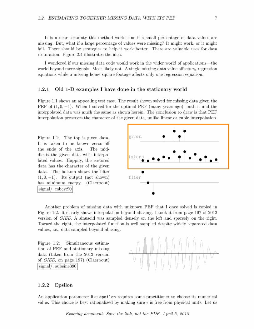
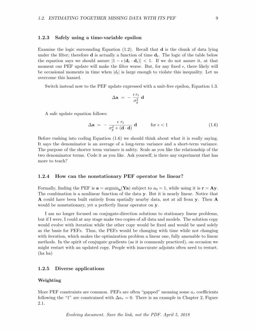
Figure 1.1 shows an appealing test case. The result shown solved for missing data given thePEF of (1, 0,�1). When I solved for the optimal PEF (many years ago), both it and theinterpolated data was much the same as shown herein. The conclusion to draw is that PEFinterpolation preserves the character of the given data, unlike linear or cubic interpolation.
Figure 1.1: The top is given data.It is taken to be known zeros o↵the ends of the axis. The mid-dle is the given data with interpo-lated values. Happily, the restoreddata has the character of the givendata. The bottom shows the filter(1, 0,�1). Its output (not shown)has minimum energy. (Claerbout)signal/. mbest90
Another problem of missing data with unknown PEF that I once solved is copied inFigure 1.2. It clearly shows interpolation beyond aliasing. I took it from page 197 of 2012version of GIEE. A sinusoid was sampled densely on the left and sparsely on the right.Toward the right, the interpolated function is well sampled despite widely separated datavalues, i.e., data sampled beyond aliasing.
Figure 1.2: Simultaneous estima-tion of PEF and stationary missingdata (taken from the 2012 versionof GIEE, on page 197) (Claerbout)signal/. subsine390
1.2.2 Epsilon
An application parameter like epsilon requires some practitioner to choose its numericalvalue. This choice is best rationalized by making sure ✏ is free from physical units. Let us
Evolving document. Save the link, not the PDF. April 5, 2018

8 CHAPTER 1. NONSTATIONARY SCALAR SIGNALS
now attend to units. From the past of y, the filter a predicts the future of y, so a itselfmust be without physical units. The data yt might have units of voltage. Its predictionerror rt has the same units. To repair the units in ✏ we need something with units of voltagesquared for the denominator. Let us take it to be the variance �2
y . You might compute itglobally for your whole data set y, or you could compute it by leaky integration (such as�2
t .99�2t�1 + .01y2
t ) to adjust itself with the nonstationary changes in data yt. The filterupdate �a with a unit-free ✏ is:
�a = � ✏ rt
�2y
d (1.3)
That is the story for epsilonA in the code above. For the missing data adaptation rate,epsilonY, no normalization is required because r(t) and y(t) have the same physicalunits; therefore the missing data yt�⌧ updates are scaled from the residual rt by the unit-free epsilonY.
Epsilon ✏ is the fractional change to the filter at each time step. In a process called“leaky integration,” any long-range average of the filter at time t is reduced by the (1� ✏)factor; then it is augmented by ✏ times a current estimate of it. After � steps, the influenceof any original time is reduced by the factor (1 � ✏)�. Setting that to 1/e = 1/2.718says (1 � ✏)� = 1/e. Taking the natural logarithm, 1 = �� ln(1 � ✏) ⇡ �✏, so to goodapproximation
✏ = 1/� (1.4)
By the well known property of exponentials, half the area in the decaying signal appearsbefore the distance �—the other half after.
I often think of the memory function (1� ✏)t as a rectangle function of length �. Leastsquares analysis begins with the idea that there should be more regression equations thanunknowns. Therefore, � should roughly exceed the number of filter coe�cients ntau. Toavoid overfitting, I suggest beginning with � = 100⇥ ntau.
There is a pitfall in the paragraph above. With synthetic data, you may have runs ofzero values. These do not count as data. Then, you need a bigger � because the zeros donot provide the needed information.
Mathematicians are skilled at dealing with the stationary case. They are inclined toconsider all residuals rt to carry equal information. They may keep a running average mt
of a residual rt by the identity (proof by induction):
mt =t� 1
tmt�1 +
1t
rt =1t
tX
k=1
rk (1.5)
This equation suggests that an ✏ decreasing proportional to 1/t (which is like � proportionalto t) may in some instances be a guide to practice, although it o↵ers little guidance fornonstationarity other than that ✏ should be larger; it should drop o↵ less rapidly than does1/t.
Given an immense amount of data, a “learning machine” should be able to come upwith a way of choosing the adaptivity rate ✏. But, besides needing an immense amount ofdata, learning machines are notoriously fragile. We should try conjuring up some physi-cal/geometric concepts for dealing with the kind of nonstationarity that our data exhibits.With such concepts we should require far less data to achieve more robust results. We needexamples to fire up our imaginations.
Evolving document. Save the link, not the PDF. April 5, 2018
1.2. ESTIMATING TOGETHER MISSING DATA WITH ITS PEF 9
1.2.3 Safely using a time-variable epsilon
Examine the logic surrounding Equation (1.2). Recall that d is the chunk of data lyingunder the filter; therefore d is actually a function of time dt. The logic of the table belowthe equation says we should assure |1 � ✏ (dt · dt)| < 1. If we do not assure it, at thatmoment our PEF update will make the filter worse. But, for any fixed ✏, there likely willbe occasional moments in time when |dt| is large enough to violate this inequality. Let usovercome this hazard.
Switch instead now to the PEF update expressed with a unit-free epsilon, Equation 1.3.
�a = � ✏ rt
�2y
d
A safe update equation follows:
�a = � ✏ rt
�2y + (d · d)
d for ✏ < 1 (1.6)
Before rushing into coding Equation (1.6) we should think about what it is really saying.It says the denominator is an average of a long-term variance and a short-term variance.The purpose of the shorter term variance is safety. Scale as you like the relationship of thetwo denominator terms. Code it as you like. Ask yourself, is there any experiment that hasmore to teach?
1.2.4 How can the nonstationary PEF operator be linear?
Formally, finding the PEF is a = argmina(Ya) subject to a0 = 1, while using it is r = Ay.The combination is a nonlinear function of the data y. But it is nearly linear. Notice thatA could have been built entirely from spatially nearby data, not at all from y. Then Awould be nonstationary, yet a perfectly linear operator on y.
I am no longer focused on conjugate-direction solutions to stationary linear problems,but if I were, I could at any stage make two copies of all data and models. The solution copywould evolve with iteration while the other copy would be fixed and would be used solelyas the basis for PEFs. Thus, the PEFs would be changing with time while not changingwith iteration, which makes the optimization problem a linear one, fully amenable to linearmethods. In the spirit of conjugate gradients (as it is commonly practiced), on occasion wemight restart with an updated copy. People with inaccurate adjoints often need to restart.(ha ha)
1.2.5 Diverse applications
Weighting
More PEF constraints are common. PEFs are often “gapped” meaning some a⌧ coe�cientsfollowing the “1” are constrained with �a⌧ = 0. There is an example in Chapter 2, Figure2.1.
Evolving document. Save the link, not the PDF. April 5, 2018

10 CHAPTER 1. NONSTATIONARY SCALAR SIGNALS
In reflection seismology, t2 gain and debubble do not commute. Do the physics right byapplying debubble first; then get a bad answer (because late data has been ignored). Dothe statistics right; apply gain first; then violate the physics. How do we make a propernonstationary inverse problem? I think the way is to merge the t2 gain with the ✏.
Change in variables
Because all we need to do is keep d · d = d⇤d positive, we immediately envision moregeneral linear changes of variables in which we keep d⇤B⇤Bd positive, implying the update�a = �✏ rt d⇤B⇤B. I conceive no example for that yet.
Wild and crazy squeezing functions
The logic leading up to Equation (1.2) requires only that we maintain polarity of theelements in that expression. Commonly, residuals like r are often squeezed down from the`2-norm derivative r, to their `1 derivative, sgn(r) = r/|r|, or the derivative of the hyperbolicpenalty function, softclip(r). Imagine an arbitrary squeezing function RandSqueeze() thatsqueezes its argument by an arbitrary polarity-preserving squeezing function. Each ⌧ mighthave its own RandSqueeze⌧ () mixing signum() and softclip() and the like. The possibilitiesare bewildering. We could update PEFs with the following:
�a⌧ = � ✏ RandSqueeze(rt) RandSqueeze⌧ (yt�⌧ ) (1.7)
Recall the real estate application. It seems natural that each of the various columns withtheir diverse entries (bathrooms, square footages) would be entitled to its own RandSqueeze⌧ ().Given enough data, how would we identify the RandSqueeze⌧ () in each column?
Deconvolution of sensible data mixed with giant spikes
The di↵erence between sgn(rt) and sgn(yt�⌧ ) is interesting. Deconvolution in the presenceof large spike noise is improved using sgn(rt) to downplay predicting corrupted data. Itis also improved by downplaying—with sgn(yt�⌧ )—regression equations that use corrupteddata to try predicting good data. On the other hand, because a humongous data valueis easy to recognize, we might more simply forget squeezing and mark such a location asmissing data value.
Convex functions do not have banana-shaped contours, a problem for many method-ologies, but not a problem herein. However, arbitrary squeezing and stretching functionscould lead to multiple minima.
The wide world of applications
What is the most general formulation? With vector-valued signals after Chapter 3 wemay find unexpected opportunities, such as vorticity in the ocean1, or Alfven waves in theionosphere. In time, diverse applications will crop up.
1 See the youtube for “Perpetual ocean.”
Evolving document. Save the link, not the PDF. April 5, 2018

1.2. ESTIMATING TOGETHER MISSING DATA WITH ITS PEF 11
1.2.6 My favorite wavelet for modelers
I digress to view current industrial marine wavelet deconvolution. Because acoustic pressurevanishes on the ocean surface, upcoming waves reflect back down with opposite polarity.This reflection happens twice, once at the air gun (about 10 meters deep), and once againat the hydrophones yielding roughly a second finite-di↵erence response called a “ghost.”Where you wish to see an impulse on a seismogram, instead you see this ghost.
The Ricker wavelet, a second derivative of a Gaussian, is often chosen for modeling.Unfortunately, the Gaussian function is not causal (not vanishing before t = 0). A morenatural choice derives from the Futterman wavelet (GIEE) which is a causal representationof the spectrum exp(�|!|t/Q) where Q is the quality constant of rock. Figure 1.3 shows theFutterman wavelet and also its second finite di↵erence. I advocate this latter wavelet formodelers because it is solidly backed by theory; and I often see it on data. The carry-awaythought is that the second derivative of a Gaussian is a three-lobed wavelet, while that ishardly true of the second derivative of a Futterman wavelet.
Figure 1.3: The causal constant Q response and its second finite di↵erence. The first twolobes are approximately the same height, but the middle lobe has more area. That third lobeis really small. Its smallness explains why the water bottom could seem a Ricker wavelet(second derivative of a Gaussian) while the top of salt would seem a doublet. (Claerbout)signal/. futter
1.2.7 Sparse decon results that I aspire to reconquer
Antoine Guitton (Guitton and Claerbout, 2015) analyzed five data sets getting amazingresults on all five. Two are shown in Figures 1.4 and 1.5. The clarity of polarity in everycase is wonderful for geologic interpretation.
Guitton’s examples were done with a stationary theory that allows the inverse shotwavelet being slightly noncausal. This suggests we should always try to spike not at thewavelet onset (which is what PEFs do), but somewhere more like the center lobe of theGaussian, namely, at the second lobe of the second derivative of the Futterman.
The nonstationary method has the ability to seek sparseness as Guitton did with thehyperbolic penalty function. Unfortunately for us (and many others before us) PEF outputs
Evolving document. Save the link, not the PDF. April 5, 2018
12 CHAPTER 1. NONSTATIONARY SCALAR SIGNALS
lose their whiteness when extended non causally. But, the goal of lucid polarity is a trulyrewarding one.
Guitton’s work did not extend readily to wider shot-hydrophone separations, a featurenaturally exploitable by the nonstationary approach. If we could get everything together,we could reasonably hope to make millions. We should begin guessing!
As a side issue, for each travel time depth ⌧ = z/v, we wish the phase correction ofexp(�|!|⌧/Q). Is that easy (like Stolt migration) or harder like downward continuation?Hmm. In any case it is not di�cult.
REFERENCES
Claerbout, J., 2014, Geophysical image estimation by example: Lulu.com.Guitton, A. and J. Claerbout, 2015, Nonminimum phase deconvolution in the log domain:
A sparse inversion approach: GEOPHYSICS, 80, WD11–WD18.Resnick, M., 2017, Lifelong Kindergarten: Cultivating Creativity through Projects, Passion,
Peers, and Play: The MIT Press, Cambridge, MA.
Evolving document. Save the link, not the PDF. April 5, 2018

1.2. ESTIMATING TOGETHER MISSING DATA WITH ITS PEF 13
Figure 1.4: Gulf of Mexico. Top is before sparse decon, bottom after. Between 2.25s to2.70s, the right side is salt (no reflectors). Notice salt top reflection is white, bottom black.Notice that sparse decon has eliminated bubble reverberation in the reflection-free salt zone(as well as elsewhere). (Antoine Guitton) signal/. antoineGOM2
Evolving document. Save the link, not the PDF. April 5, 2018

14 CHAPTER 1. NONSTATIONARY SCALAR SIGNALS
Figure 1.5: O↵shore west Australia. Notice how the sparse decon creates many eventsthat are pure white or pure black. White denotes a hard reflector, black a soft one.signal/. antoineAustralia
Evolving document. Save the link, not the PDF. April 5, 2018

Chapter 2
Spatial deconvolution
2.1 TIME AND SPACE
1A streaming 1-D prediction filter is a decaying average of earlier prediction filters; however,these earlier filters need not all be saved in memory. Because they vary smoothly, we maysimply use the most recent one. Call it a. In two dimensions, a becomes some average of itsprevious value on each of its two axes. For example, instead of updating from the previousmoment a(t��t, x), we could update from the previous location a(t, x��x). That wouldbe learning over x while filtering over t. More generally, an update could leap from a basethat is a weighted average over time and space. We would update a a + �a with thefollowing:
a = a(t��t, x)�2
t
�2t + �2
x+ a(t, x��x)
�2x
�2t + �2
x(2.1)
Notice that the weights sum to unity. The averaging region is an area roughly �x�t pixelssquared in size. The coding requires not only saving a at the previous time, it requires atthe previous x, namely at x � �x, all lags of a saved over all time. The memory cost isnt ⇥ n⌧ , not bad.
In 3-D, it looks like we will need a plane of saved PEFs. In higher dimensional spaces,we need store PEFs only in the zone of the transition from the filtered to the unfiltered.Thus, in 5-D, we need to store a 4-D volume of PEFs. Do not let that trouble you though.Because the PEFs are generally smoothly variable, they can be linearly interpolated froma sparse grid.
PEFs on the previous trace a(t, x � �x) can be smoothed symmetically on the timeaxis. Such smoothing expands the averaging region from the quadrant behind (t, x) to thehalfspace behind x.
Stationary decon should remove a shot waveform. Nonstationary decon starts fromthere but has the added opportunity of removing the waveform of the propagating wave.It evolves with travel time (Q and forward scattered multiples). It also evolves with space,especially shot to receiver separation.
1Drawn from Fomel et al. (2016).
15

16 CHAPTER 2. SPATIAL DECONVOLUTION
2.1.1 Bubble removal
The internet easily yields slow-motion video of gun shots under water. Perhaps unex-pectedly, the rapidly expanding exhaust gas bubble soon slows; then, collapses to a point,where it behaves like a second shot—repeating again and again. This reverberation pe-riod (the interval between collapses) for exploration air guns (“guns” shooting bubblesof compressed air) is herein approximately 120 milliseconds. Imagers hate it. Inter-preters hate it. Figure 2.1 shows marine data and a gapped PEF applied to it. It is alarge gap, 80 milliseconds (ms), or 80/4=20 samples on data sampled at 4 ms, actually,�a = (1, 0, 0,more zeros, 0, a20, a21, · · · , a80).
Figure 2.1: Debubble done by the nonstationary method. Original (top), debubbled (bot-tom). On the right third of the top plot, prominent bubbles appear as three quasihorizontalblack bands between times 2.4s and 2.7s. Blink overlay display would make it more evidentthat there is bubble removal everywhere. (Joseph Jennings) image/. debubble-ovcomp
Evolving document. Save the link, not the PDF. April 5, 2018

2.1. TIME AND SPACE 17
2.1.2 Two-dimensional PEF
We have seen 1-D PEFs applied to 2-D data. Now for 2-D PEFs. Signal analysis extends toimage analysis quite easily except for the fact that the spike on the PEF is not in the middleor on a corner of the 2-D filter array but on its side. This old knowledge is summarized inAppendix 5.1.2 Why 2-D PEFs have white output.
Figure 2.2: A PEF is a functionof lag a(tl,xl). It is lying back-ward herein—shown as crosscorre-lating seismic data with t down,x to the right. On the filter, ⌧runs up, x runs left. (Claerbout)image/. pef2-d
a(2,2) a(2,1) a(2,0)a(1,2) a(1,1) a(1,0)a(0,2) a(0,1) 1.0a(-1,2) a(-1,1) 0a(-2,2) a(-2,1) 0
Unlike the 1-D code herein, we use negative subscripts on time. As in 1-D, the PEFoutput is aligned with its input because a(0,0)=1. To avoid filters trying to use o↵-endinputs, no output is computed (first two loops) at the beginning of the x axis nor at bothends of the time axis. At three locations below the lag loops (tl,xl), cover the entirefilter. First, the residual r(t,x) calculation (# Filter) is simply the usual 1-D convolutionseen additionally on the 2-axis. Next, the adjoint follows the usual rule of swapping inputand output spaces. (Then the constraint line preserves not only the 1.0, but also the zerospreceeding it.) Finally, the update line a-=da is trivial.
# CODE = 2-D PEFread y( 0...nt , 0...nx) # data
r( 0...nt , 0...nx) =0. # residual = PEF outputa(-nta...nta, 0...nxa)=0. # filter Illustrated size is a( -2...2, 0...2).a( 0 , 0 )=1.0 # spike
do for x = nxa to nxdo for t = nta to nt-nta
do for xl= 0 to +nxado for tl= -nta to +nta
da(tl,xl) = 0.r (t ,x ) += a(tl,xl) * y(t-tl, x-xl) # Filter
do for xl= 0 to +nxado for tl= -nta to +nta
da(tl,xl) += r(t , x) * y(t-tl, x-xl) # Adjoint
do for tl= -nta to 0 # Constraintsda(tl, 0) = 0.
do for xl= 0 to +nxado for tl= -nta to +nta
a (tl,xl) -= da(tl,xl) * epsilon/variance # Update
This code whitens (flattens) nonstationary spectra in the 2-D frequency (!, kx)-space. Thelocal autocorrelation tends to a delta function in 2-D lag (tl,tx)-space. Everybody’s 2-Dimage estimations need code like this code to achieve IID residuals.
Evolving document. Save the link, not the PDF. April 5, 2018
18 CHAPTER 2. SPATIAL DECONVOLUTION
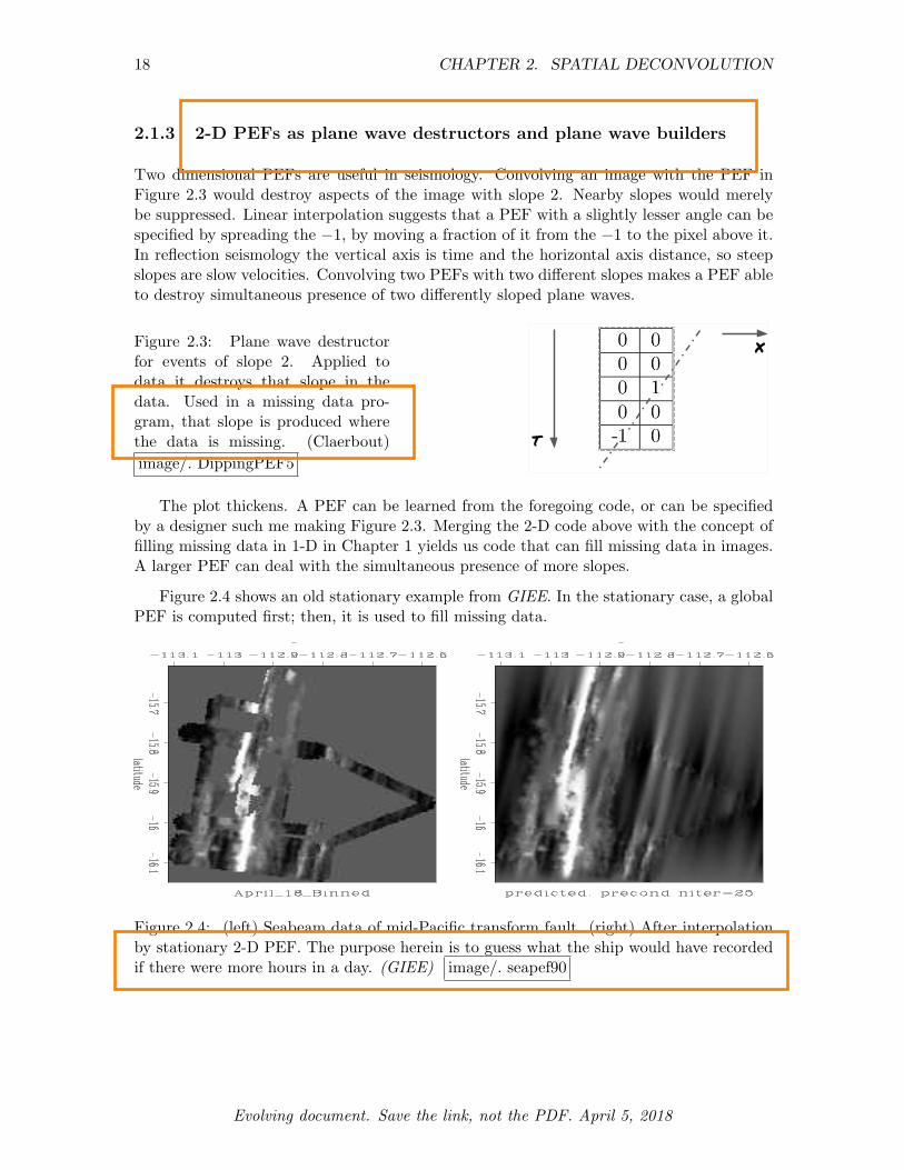
2.1.3 2-D PEFs as plane wave destructors and plane wave builders
Two dimensional PEFs are useful in seismology. Convolving an image with the PEF inFigure 2.3 would destroy aspects of the image with slope 2. Nearby slopes would merelybe suppressed. Linear interpolation suggests that a PEF with a slightly lesser angle can bespecified by spreading the �1, by moving a fraction of it from the �1 to the pixel above it.In reflection seismology the vertical axis is time and the horizontal axis distance, so steepslopes are slow velocities. Convolving two PEFs with two di↵erent slopes makes a PEF ableto destroy simultaneous presence of two di↵erently sloped plane waves.
Figure 2.3: Plane wave destructorfor events of slope 2. Applied todata it destroys that slope in thedata. Used in a missing data pro-gram, that slope is produced wherethe data is missing. (Claerbout)image/. DippingPEF5
t
x
The plot thickens. A PEF can be learned from the foregoing code, or can be specifiedby a designer such me making Figure 2.3. Merging the 2-D code above with the concept offilling missing data in 1-D in Chapter 1 yields us code that can fill missing data in images.A larger PEF can deal with the simultaneous presence of more slopes.
Figure 2.4 shows an old stationary example from GIEE. In the stationary case, a globalPEF is computed first; then, it is used to fill missing data.
Figure 2.4: (left) Seabeam data of mid-Pacific transform fault. (right) After interpolationby stationary 2-D PEF. The purpose herein is to guess what the ship would have recordedif there were more hours in a day. (GIEE) image/. seapef90
Evolving document. Save the link, not the PDF. April 5, 2018

2.1. TIME AND SPACE 19
2.1.4 Example of a 2-D PEF applied to a seismic section
Figure 2.5 shows the world’s first “industrial scale” nonstationary 2-D prediction error. Itwas the principal product of a summer research group led by Bob Clapp (Ruan et al., 2015).It demonstrates a 2-D nonstationary deconvolution based on the idea of using a coarse gridto store many 2-D PEFs. Someone should try it with the code above which is much simpler.This data set and others used by Guitton (Guitton and Claerbout, 2015) are available fortesting the streaming ideas of this tutorial.
Figure 2.5: A common depth point (CDP) stack before and after 2-D decon. Its goal isto suppress predictable events. It does not attempt to give zero strength to the layers, butto give all slopes uniform strength. That is the meaning of whiteness in (!, kx)-space. Theresidual hyperbolas are called “di↵ractions.” (Ruan et al., 2015) image/. wgstack
2.1.5 Stretch matching
Sometimes we have two signals that are nearly the same but for some reason, one is stretcheda little from place to place. Tree rings seem an obvious example. I mostly encounterseismograms where a survey was done both before and after oil and gas production, so thereare stretches along the seismogram that have shrunken or grown. A decade or two back,navigation was not what it is now, especially for seismograms recorded at sea. Navigationwas one reason, tidal currents are another. Towed cables might not be where intended.So, signals might shift in both time and space. A first thought is to make a runningcrosscorrelation. The trouble is, crosscorrelation tends to square spectra which diminishesthe high frequencies, those being just the ones most needed to resolve small shifts. Let usconsider the time-variable filter that best converts one signal to the other.
Take the filter a to predict signal x from signal y. Either signal might lag the other.Take the filter to be two-sided, [a(-9),a(-8),...,a(0),a(1),...,a(9)]. Let us beginfrom a(0)=1, but not hold that as a constraint.
Evolving document. Save the link, not the PDF. April 5, 2018

20 CHAPTER 2. SPATIAL DECONVOLUTION
r(...) = 0. # CODE = NONSTATIONARY EXTRAPOLATION FILTERa(...) = 0.a( 0 ) = 1.do over time t { # r(t) = nonstationary extrapolation error
do i= -ni, nir(t) += a(i) * y(t-i) - x(t) # forward
do i= -ni, nia(i) -= r(t) * y(t-i) * epsilon # adjoint
do i= -ni, nishift(t) = i * a(i)
}
The last loop is to extract from the filters a time shift. Here I have simply computed themoment. That would be correct if signals x and y had the same variance. If not, I leave itto you calculate their standard deviations �x and �y and scale the shift in the code aboveby �x/�y thus yielding the shift in pixels.
Do not forget, if you have only one signal, or if it is short, you likely should loop overthis code multiple times while decreasing epsilon.
Besides time shifting, the filtering operator has the power of gaining and of changingcolor. Suppose, for example that brother y and sister x each recited a message. Thisfiltering could not only bring them into synchronization, it would raise his pitch. Likewisein 2-D starting from their photos, he might come out resembling her too much!
2.2 DISJOINT REGIONS OF SPACE
2.2.1 Geostatistics
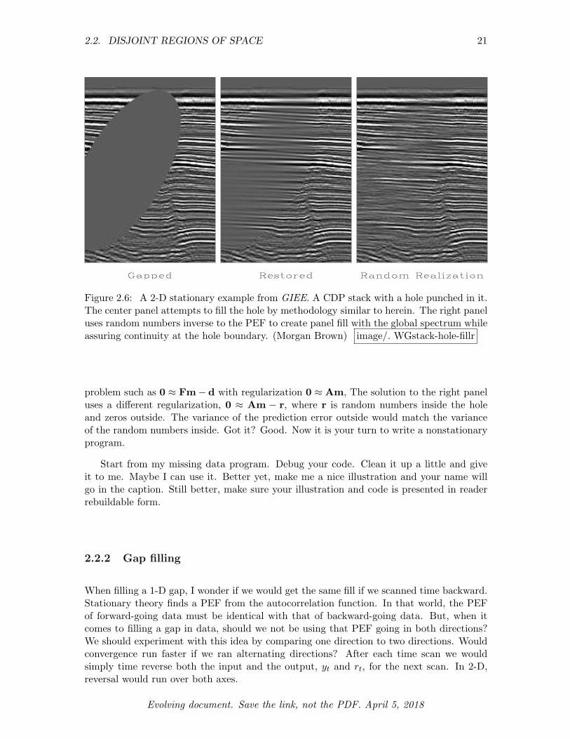
Figure 2.6 illustrates using PEF technology refilling an artificial hole in an image of the Gulfof Mexico. This illustration (taken from GIEE) uses mature stationary technology. Thecenter panel illustrates filling in missing data from knowledge of a PEF gained outside thehole. The statistics at the hole in the center panel are weaker and smoother than the statis-tics of the surrounding data. Long wavelengths have entered the hole but diminish slowlyin strength as they propagate away from the edges of known data. Shorter wavelengthsare less predictable and diminish rapidly to zero as we enter the unknown. Actually, it isnot low frequency but narrow bandedness that enables projection far into the hole from itsboundaries.
The right panel illustrates a concept we have not covered. This panel has the samespectrum inside the hole as outside. Nice. And, it does not decay in strength going inwardfrom the boundaries of the hole. Nice. Before I ask you which you prefer, the central panelor the right panel, I should tell you that the right panel is one of millions of panels thatcould have been shown. Each of the millions uses a di↵erent set of random numbers. Astatistician (i.e., Albert Tarantola) would say the solution to a geophysical inverse problemis a random variable. The center panel is the mean of the random variable. The right panelis one realization of the many possible realizations. The average of all the realizations isthe center panel.
Geophysicists tend to like the center panel; geostatisticians tend to prefer an ensembleof solutions, such as the right panel. In stationary theory, the center panel is a solution to a
Evolving document. Save the link, not the PDF. April 5, 2018
2.2. DISJOINT REGIONS OF SPACE 21
Figure 2.6: A 2-D stationary example from GIEE. A CDP stack with a hole punched in it.The center panel attempts to fill the hole by methodology similar to herein. The right paneluses random numbers inverse to the PEF to create panel fill with the global spectrum whileassuring continuity at the hole boundary. (Morgan Brown) image/. WGstack-hole-fillr
problem such as 0 ⇡ Fm� d with regularization 0 ⇡ Am, The solution to the right paneluses a di↵erent regularization, 0 ⇡ Am � r, where r is random numbers inside the holeand zeros outside. The variance of the prediction error outside would match the varianceof the random numbers inside. Got it? Good. Now it is your turn to write a nonstationaryprogram.
Start from my missing data program. Debug your code. Clean it up a little and giveit to me. Maybe I can use it. Better yet, make me a nice illustration and your name willgo in the caption. Still better, make sure your illustration and code is presented in readerrebuildable form.
2.2.2 Gap filling
When filling a 1-D gap, I wonder if we would get the same fill if we scanned time backward.Stationary theory finds a PEF from the autocorrelation function. In that world, the PEFof forward-going data must be identical with that of backward-going data. But, when itcomes to filling a gap in data, should we not be using that PEF going in both directions?We should experiment with this idea by comparing one direction to two directions. Wouldconvergence run faster if we ran alternating directions? After each time scan we wouldsimply time reverse both the input and the output, yt and rt, for the next scan. In 2-D,reversal would run over both axes.
Evolving document. Save the link, not the PDF. April 5, 2018
22 CHAPTER 2. SPATIAL DECONVOLUTION
2.2.3 Rapid recognition of a spectral change
This booklet begins with with the goal of escaping the strait jacket of stationarity, intendingmerely to allow for slowly variable spectral change. Real life, of course has many importantexamples in which a spectral change is so rapid that our methods cannot adapt to it—imagine you are tracking a sandstone. Suddenly, you encounter a fault with shale on theother side and permeability is blocked—this could be bad fortune or very good fortune!
Warming up to an unexpectedly precise measurement of location of spectral changeconsider this 1-D example: Let T = 1 and o = �1. The time function
(...., T, T, T, o, o, o, T, T, T, o, o, o, T, T, T, o, o, T, T, o, o, T, T, o, o, T, T, o, o....)
begins with period 6 and abruptly switches to period 4. The magnitude of the predictionerror running to the right is quite di↵erent from the one running to the left. Runningright, the prediction error is approximately zero, but, it suddenly thunders at the momentof spectral change, thunder gradually dying away again as the PEF adapts. Running left,again there is another thunder of prediction error; but, this thunder is on the oppositeside of the abrupt spectral change. Having both directions is the key to defining a sharpboundary between the two spectra. Let the prediction variance going right be �right andgoing left be �left. The local PEF is then defined by a weighted average of the two PEFs.
a =�right
�right + �leftaleft +
�left
�right + �leftaright (2.2)
A weight is big where the other side has big error variance. The width of the zone oftransition is comparable to the duration of the PEFs, much shorter than the distance ofadaptation. This is an amazing result. We have sharply defined the location for the spectralchange even though the PEF estimation cannot be expected to adapt rapidly to spectralchanges. Amazing! This completes your introduction for the image of Lenna, Figure 2.8.
2.2.4 Boundaries between regions of constant spectrum
There is no direct application to predicting financial markets. But, with recorded data, onecan experiment with predictions in time forward, and backward. Including space with timemakes it more intriguing. In space, there is not only forwards and backwards but sidewaysand at other angles. The PEF idea in 3-D (Figure 2.7) shows that sweeping a plane (the topsurface) upward through a volume transforms an unfiltered upper half-space to a filteredlower one. Whatever trajectory the sweep takes, it may also be done backward, even atother angles.
You are trying to remove noise from the test photo of Lenna (Figure 2.8). Your sweepabruptly transitions from her smooth cheek to her straight hair, to the curly fabric of herhat. To win this competition, you surely want sweeps in opposite directions or even moredirections. Fear not that mathematics limits us to slow spectral transitions. The location ofa sharp spectral transition can be defined by having colliding sweeps, each sweep abruptlylosing its predictability along the same edge. But Lenna is not ours yet.
How should we composite the additional sweeps that are available in higher dimensionalspaces? Obviously, we get two sweep directions for each spatial dimension; but, more might
Evolving document. Save the link, not the PDF. April 5, 2018

2.2. DISJOINT REGIONS OF SPACE 23
Figure 2.7: The coe�cients in a 3-DPEF. (GIEE) image/. 3dpef
1
be possible at 45� angles or with hexagonal coordinates. I would start with an unnormalizedweight from each ith pass of N passes by the inverse of a smoothing of the PEF outputvariance.
wi = 1/ < �i > (2.3)
Then, I would take the PEF at every point in space by the following
a =PN
i wi aiPNi wi
(2.4)
I confess, all of this is pretty speculative, and I have doubts about how to average PEFsin di↵erent directions. In 1-D, we have some feeling for it because stationary theory tellsus forward and backward PEFs are the same. Something similar might happen in 2-D,but I have doubts about merging a north-south PEF information with an east-west PEFinformation.
Figure 2.8: Lenna, a widelyknown photo used for testing en-gineering objectives in photometry.(Wikipedia) image/. Lenna
Evolving document. Save the link, not the PDF. April 5, 2018
24 CHAPTER 2. SPATIAL DECONVOLUTION
2.2.5 What physical phenomena gives the spectra of a 3-D PEF?
Although it is clear how to fit a single 3-D PEF to data, it might not be relevant to seismicdata. Waves fill a volume with pancakes, not with noodles. When I see 3-D data, y(t, x, y),I visualize it containing planes. A plane in 3-D looks like a line in both (t, x) and (t, y)space. It is more e�cient to fit two planes each with a 2-D PEF [a(t, x), b(t, y)] than with asingle 3-D PEF a(t, x, y). If you have been thinking about a regularization, it now becomestwo regularizations. What physical 3-D fields call for 3-D PEFs? I could guess, but this isnot the time and place.
REFERENCES
Fomel, S., J. Claerbout, S. Levin, and R. Sarkar, 2016, Streaming nonstationary predictionerror (II): SEP-Report, 163, 271–277.
Guitton, A. and J. Claerbout, 2015, Nonminimum phase deconvolution in the log domain:A sparse inversion approach: GEOPHYSICS, 80, WD11–WD18.
Ruan, K., J. Jennings, E. Biondi, R. G. Clapp, S. A. Levin, and J. Claerbout, 2015, Indus-trial scale high-performance adaptive filtering with pef applications: SEP-Report, 160,177–188.
Evolving document. Save the link, not the PDF. April 5, 2018

Chapter 3
Vector-valued signals
1We have done much with PEFs on scalar-valued signals. Vector-valued signals are for3-component seismographs and the like. The idea of deconvolution with a PEF extendsto multicomponent signals. In ideal geometries, di↵erent wave types arrive on di↵erentchannels; but in real life, wave types get mixed. Pressure waves tend to arrive on verti-cal seismographs, and shear waves arrive on horizontals; but, dipping waves corrupt eachchannel with the other. The main goal herein is to disentangle this channel crosstalk.
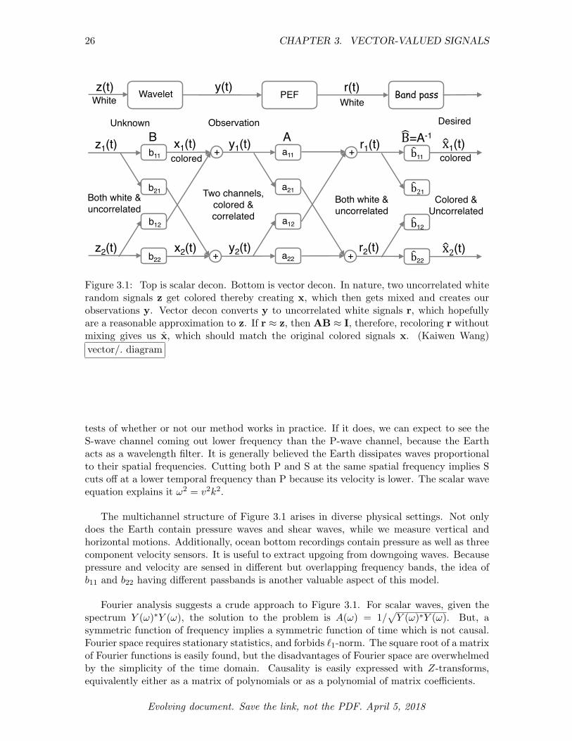
Scalar blind deconvolution is widely used in the seismic survey industry. The simpleinformation flow in the upper quarter of Figure 3.1 is pretty much what we have done inChapter 1 with the addition of the bandpass filter at the end. Oversimplifying, the ideais that Earth layers have random densities (impedances), therefore random echo polaritiesat a fine scale. This layering zt gets smeared by the source wavelet, which is not an idealimpulse, instead being a mixture of air bubbles, ghosts, and weathered-layer reverberationsleading to the observed output yt. Those corrupting processes amount to causal filters, bestundone with a PEF producing the output rt. The bandpass filter at the end is there forsubjective reasons, mainly we do not want to clutter our view with the highest possiblefrequency that a grid can hold because we know it is just noise. A popular alternative tothe bandpass filter is gapping the PEF. Instead of limiting high frequencies, it does muchthe same by broadening the autocorrelation spike of the “white” output.
3.0.6 Multi channels == vector-valued signals
Widespread adaptation of multicomponent recorders leads to new opportunities indicatedby the lower bulk of Figure 3.1. Hypothetical statistically independent channels z1 andz2 become colored making our ideal unpolluted channels x1 and x2, which unfortunately“crosstalk” before giving us our observations y1 and y2. Learning herein the theory of matrixvalued PEFs, we design a matrix of filters, say A = aij attempting to achieve the originalpurity of z. Normally, we do not wish to achieve the pure whiteness of z. Rather thanapply a bandpass filter herein, we use our estimates b11 and b22 to find x as our attempt torestore the original colored signals x.
Others may make other choices, but we are choosing to display x for a reason. We want1This chapter draws from (Claerbout and Wang, 2017).
25
26 CHAPTER 3. VECTOR-VALUED SIGNALS
z1(t)
z2(t)
y1(t)
y2(t)
r1(t)
r2(t)
b11
b21
b12
b22
a11
a21
a12
a22
+
+
+
+
x1(t)
x2(t)
Unknown Observation Desired
Two channels, colored & correlated
Both white & uncorrelated
Waveletz(t) y(t) r(t)White White
b"22
b"12
b"21
b"11
x%1(t)
x%2(t)
Colored &Uncorrelated
Band passPEF
B A B'=A-1
coloredcolored
Both white & uncorrelated
Figure 3.1: Top is scalar decon. Bottom is vector decon. In nature, two uncorrelated whiterandom signals z get colored thereby creating x, which then gets mixed and creates ourobservations y. Vector decon converts y to uncorrelated white signals r, which hopefullyare a reasonable approximation to z. If r ⇡ z, then AB ⇡ I, therefore, recoloring r withoutmixing gives us x, which should match the original colored signals x. (Kaiwen Wang)vector/. diagram
tests of whether or not our method works in practice. If it does, we can expect to see theS-wave channel coming out lower frequency than the P-wave channel, because the Earthacts as a wavelength filter. It is generally believed the Earth dissipates waves proportionalto their spatial frequencies. Cutting both P and S at the same spatial frequency implies Scuts o↵ at a lower temporal frequency than P because its velocity is lower. The scalar waveequation explains it !2 = v2k2.
The multichannel structure of Figure 3.1 arises in diverse physical settings. Not onlydoes the Earth contain pressure waves and shear waves, while we measure vertical andhorizontal motions. Additionally, ocean bottom recordings contain pressure as well as threecomponent velocity sensors. It is useful to extract upgoing from downgoing waves. Becausepressure and velocity are sensed in di↵erent but overlapping frequency bands, the idea ofb11 and b22 having di↵erent passbands is another valuable aspect of this model.
Fourier analysis suggests a crude approach to Figure 3.1. For scalar waves, given thespectrum Y (!)⇤Y (!), the solution to the problem is A(!) = 1/
pY (!)⇤Y (!). But, a
symmetric function of frequency implies a symmetric function of time which is not causal.Fourier space requires stationary statistics, and forbids `1-norm. The square root of a matrixof Fourier functions is easily found, but the disadvantages of Fourier space are overwhelmedby the simplicity of the time domain. Causality is easily expressed with Z-transforms,equivalently either as a matrix of polynomials or as a polynomial of matrix coe�cients.
Evolving document. Save the link, not the PDF. April 5, 2018

3.1. MULTIDIMENSIONAL PEF 27
3.1 MULTIDIMENSIONAL PEF
This mathematical model applies to one point in space, where it is based on causality andsimultaneity of the two channels responding to the world around. The two-component signalmodel herein is not suitable for two scalar signals recorded at separate locations. At separatelocations, there naturally would be time delays between the locations. If the underlyingmodel B were to introduce delay, its hypothetical inverse A would need to contain inversedelay (anticausality!). Because A, a PEF, is casual by construction, it cannot functionanticausally. Whatever A would come out of this process, it could not satisfy BA = I. Inother words, there are many ways B could contain delays without changing its covarianceBB⇤. Our inverse operator A is fundamentally based on BB⇤, which contains no phase.We get phase by insisting on causality for A.
If you are processing a string of multicomponent recorders (e.g., down a well) eachmulticomponent recorder yields statistics that may be shared and averaged with neighboringrecorders, but the signals themselves do not mix. The process described herein is simplya vector-valued, time variable linear operator. The same process could be independentlyapplied to other channels.
Delay causes the method of this paper to fail in principle. In marginal cases (tiny delay)the notion of sparsity has helped for scalar signals (Claerbout and Guitton, 2013). There isan example in Chapter 1. Minuscule delays are a promising area beyond our present scope.Di↵erential equations apply to a point in space. Their finite di↵erence representations coverslightly more than a point. There may be some ticklish but promising aspects of mergingfinite di↵erence operators with vector signals.
The multichannel model would seem to extend to three and more physical dimensionsthough we will never know until we try. Whether or not it is suitable for many channelmarket signals, I cannot predict.
3.1.1 Vector signal scaling
When components of data or model are out of scale with one another, bad things happen,such as the adjoint operator will not be a good approximation to the inverse, physicalunits may be contradictory, and the steepest descent method creep along slowly. Thesedangers would arise with vector-valued signals if the observations y1 and y2 had di↵erentphysical units such as pressure and velocity recorded from up-going and down-going waves,or, uncalibrated vertical and horizontal seismograms.
We need to prepare ourselves for channels being out of scale with one another. Thus,we scale each component of data y and residual r by dividing out their variances. Recallthat any component of a gradient may be scaled by any positive number. Such scaling ismerely a change in coordinates.
With scalar signals, we updated using �a = � (✏ r/�2y) yt�⌧ . With multiple channels, we
are a bit more cautious and allow for data variance to di↵er from prediction-error variance.More importantly, the two components of y might have di↵ering physical units. Let �r bean estimate of the standard deviation of the prediction error in each channel. The following
Evolving document. Save the link, not the PDF. April 5, 2018
28 CHAPTER 3. VECTOR-VALUED SIGNALS
code resembles this update
�a = �
✏ r
�r�y
!
yt�⌧ (3.1)
Our original code contained leaky integrations for �y and �r, but we had no vision ofdata to test that aspect. It also gave odd behavior when we adapted too rapidly. Becausewe had more pressing areas in which to direct our attention, the code exposition belowsimply replaces �y and �r by their global averages.
3.1.2 Pseudocode for vector signals
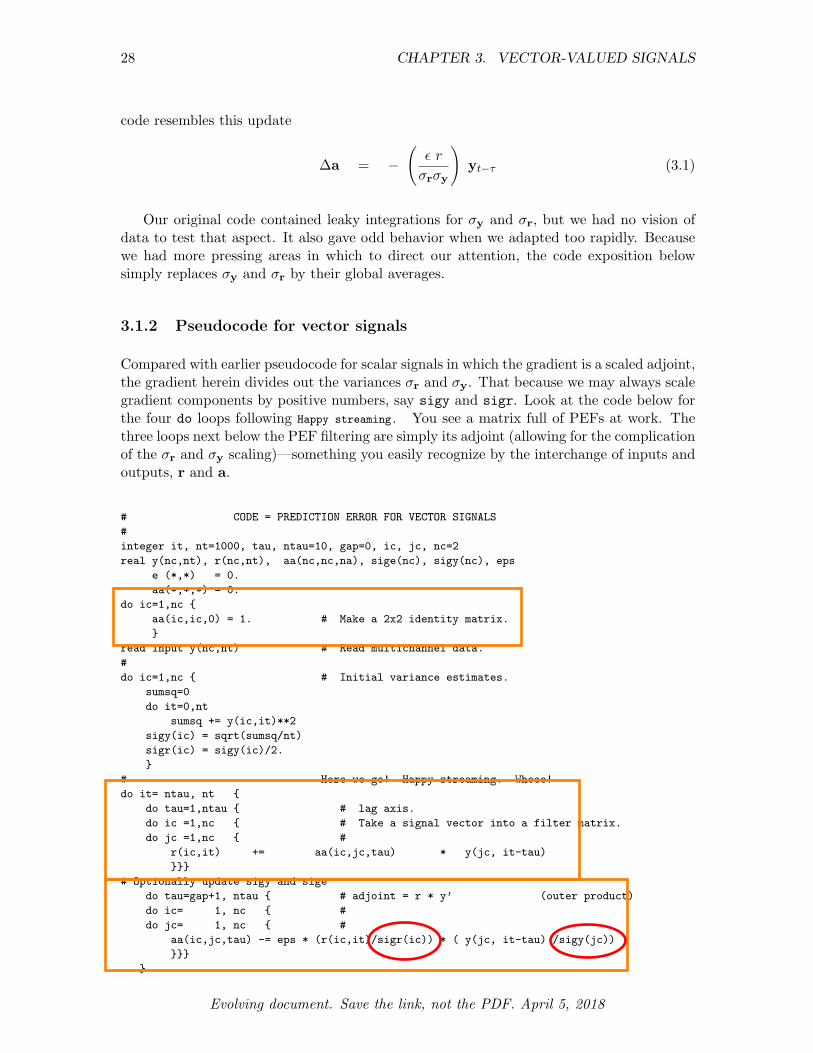
Compared with earlier pseudocode for scalar signals in which the gradient is a scaled adjoint,the gradient herein divides out the variances �r and �y. That because we may always scalegradient components by positive numbers, say sigy and sigr. Look at the code below forthe four do loops following Happy streaming. You see a matrix full of PEFs at work. Thethree loops next below the PEF filtering are simply its adjoint (allowing for the complicationof the �r and �y scaling)—something you easily recognize by the interchange of inputs andoutputs, r and a.
# CODE = PREDICTION ERROR FOR VECTOR SIGNALS#integer it, nt=1000, tau, ntau=10, gap=0, ic, jc, nc=2real y(nc,nt), r(nc,nt), aa(nc,nc,na), sige(nc), sigy(nc), eps
e (*,*) = 0.aa(*,*,*) = 0.
do ic=1,nc {aa(ic,ic,0) = 1. # Make a 2x2 identity matrix.}
read input y(nc,nt) # Read multichannel data.#do ic=1,nc { # Initial variance estimates.
sumsq=0do it=0,nt
sumsq += y(ic,it)**2sigy(ic) = sqrt(sumsq/nt)sigr(ic) = sigy(ic)/2.}
# Here we go! Happy streaming. Wheee!do it= ntau, nt {
do tau=1,ntau { # lag axis.do ic =1,nc { # Take a signal vector into a filter matrix.do jc =1,nc { #
r(ic,it) += aa(ic,jc,tau) * y(jc, it-tau)}}}
# Optionally update sigy and sigedo tau=gap+1, ntau { # adjoint = r * y’ (outer product)do ic= 1, nc { #do jc= 1, nc { #
aa(ic,jc,tau) -= eps * (r(ic,it)/sigr(ic)) * ( y(jc, it-tau) /sigy(jc))}}}
}
Evolving document. Save the link, not the PDF. April 5, 2018

3.1. MULTIDIMENSIONAL PEF 29
Now, it is easy to say that the code above is really quite trivial, but I breathed a sigh of reliefwhen Kaiwen showed me the first results. (It worked on the first try!) Before I conceivedthe calculation as explained above, I had quite a struggle attempting the derivative of aquadratic form by a matrix filter, and even more doubts that I would be able to explain myanalysis to other people, as well as a debt to Mohammed Hadidi, whose derivation showedthat my derivative was the transpose of the correct one. Then I tried thinking carefullyabout Figure 3.1. But, it was better not to think at all; instead simply code the modeling,its adjoint, and stu↵ in the residual! Phew.
3.1.3 How the conjugate gradient method came to be oversold
Textbooks often illustrate the solution to a two component regression by comparing thesteepest-descent method to the conjugate-gradient method. Conjugate gradient winninglyobtains the exact solution on the second iteration while steepest descent plods along zig-zagging an infinite number of iterations. But, is this a fair comparison? Is it not true thataxis stretching completely alters the picture? So, what exactly is the axis stretching thatmakes a more fair comparison? I suspect it is the kind of stretching done in the precedingcode with variance divisors.
3.1.4 The PEF output is orthogonal to its inputs
Let us try to understand what this program has accomplished. If the program ran a longtime in a stationary environment with a tiny ✏ eps, the filter A, namely aa(*,*,*) wouldno longer be changing. The last line of the code would then say the residual r(ic,it) isorthogonal to the fitting functions y(jc,it-tau+1). We would have a square matrix fullof such statements. The fitting functions are all channel combinations of the shifted data.That is the main ingredient to Levin’s whiteness proof for scalar signals in Chapter 5. Ibelieve it means we can presume Levin’s whiteness proof applies to vector signals. As wesubsequently see, however, the situation at zero lag does bring up something new (Choleskyfactorization).
3.1.5 Restoring source spectra
White signals are not ideal for display. Before corruption from channel 2, channel 1 hadthe spectrum of b11. Consider restoring r1 to the original spectrum, namely b11. BecauseB = A�1, we can deduce b11.
B ="
b11 b12
b21 b22
#
="
a11 a12
a21 a22
#�1
=1
a11a22 � a21a12
"a22 �a12
�a21 a11
#
(3.2)
Under the assumption that the crossover filters are less significant than the pass-throughfilters, we may simplify the result for initial trials:
b11 = a22/(a11a22 � a21a21) ⇡ 1/a11 (3.3)b22 = a11/(a11a22 � a21a21) ⇡ 1/a22 (3.4)
Evolving document. Save the link, not the PDF. April 5, 2018
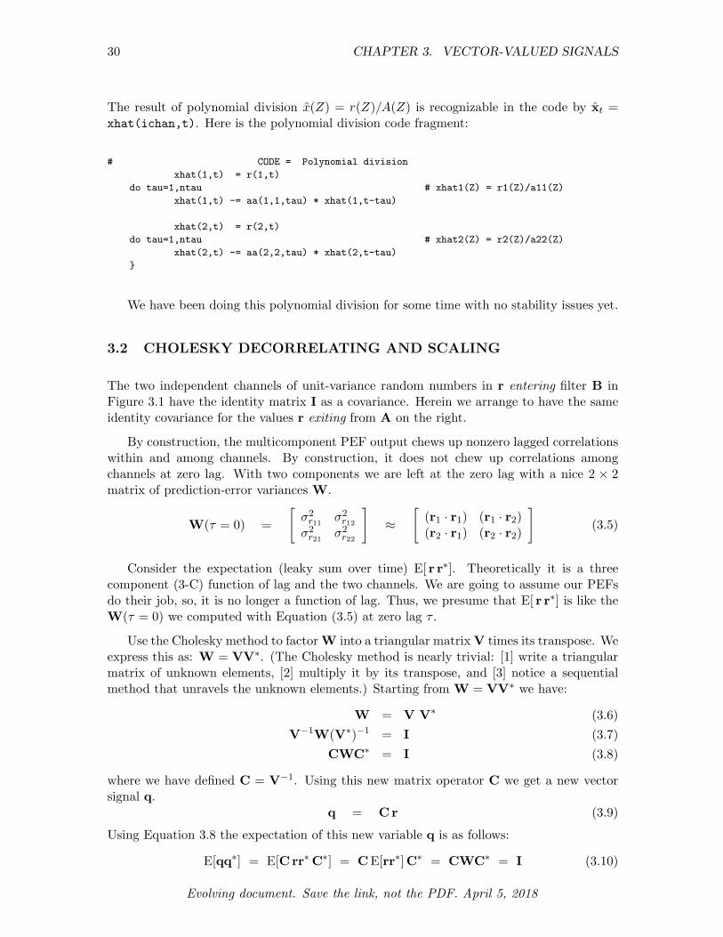
30 CHAPTER 3. VECTOR-VALUED SIGNALS
The result of polynomial division x(Z) = r(Z)/A(Z) is recognizable in the code by xt =xhat(ichan,t). Here is the polynomial division code fragment:
# CODE = Polynomial divisionxhat(1,t) = r(1,t)
do tau=1,ntau # xhat1(Z) = r1(Z)/a11(Z)xhat(1,t) -= aa(1,1,tau) * xhat(1,t-tau)
xhat(2,t) = r(2,t)do tau=1,ntau # xhat2(Z) = r2(Z)/a22(Z)
xhat(2,t) -= aa(2,2,tau) * xhat(2,t-tau)}
We have been doing this polynomial division for some time with no stability issues yet.
3.2 CHOLESKY DECORRELATING AND SCALING
The two independent channels of unit-variance random numbers in r entering filter B inFigure 3.1 have the identity matrix I as a covariance. Herein we arrange to have the sameidentity covariance for the values r exiting from A on the right.
By construction, the multicomponent PEF output chews up nonzero lagged correlationswithin and among channels. By construction, it does not chew up correlations amongchannels at zero lag. With two components we are left at the zero lag with a nice 2 ⇥ 2matrix of prediction-error variances W.
W(⌧ = 0) ="
�2r11
�2r12
�2r21
�2r22
#
⇡"
(r1 · r1) (r1 · r2)(r2 · r1) (r2 · r2)
#
(3.5)
Consider the expectation (leaky sum over time) E[ r r⇤]. Theoretically it is a threecomponent (3-C) function of lag and the two channels. We are going to assume our PEFsdo their job, so, it is no longer a function of lag. Thus, we presume that E[ r r⇤] is like theW(⌧ = 0) we computed with Equation (3.5) at zero lag ⌧ .
Use the Cholesky method to factor W into a triangular matrix V times its transpose. Weexpress this as: W = VV⇤. (The Cholesky method is nearly trivial: [1] write a triangularmatrix of unknown elements, [2] multiply it by its transpose, and [3] notice a sequentialmethod that unravels the unknown elements.) Starting from W = VV⇤ we have:
W = V V⇤ (3.6)V�1W(V⇤)�1 = I (3.7)
CWC⇤ = I (3.8)
where we have defined C = V�1. Using this new matrix operator C we get a new vectorsignal q.
q = Cr (3.9)
Using Equation 3.8 the expectation of this new variable q is as follows:
E[qq⇤] = E[Crr⇤C⇤] = CE[rr⇤]C⇤ = CWC⇤ = I (3.10)
Evolving document. Save the link, not the PDF. April 5, 2018

3.3. ROTATING FOR SPARSITY 31
This proves Cholesky meets our goals: (1) it descales, and (2) it decorrelates r at zerolag.
3.3 ROTATING FOR SPARSITY
Intrigue is what comes last, something wholly unfamiliar. As the universe marches on,things get mixed and entropy increases. We seek the opposite. Even after solving theproblem posed in Figure 3.1, the solution is unique only within an arbitrary unitary matrix.(With scalar signals the arbitrariness is in a scale factor ei�.) We get to choose the unitarymatrix U having minimum entropy r output. Luckily, this two-channel problem, althoughnonlinear, is easily amenable to a one-parameter exhaustive search. That search can bedone to maximize sparsity of the final signals. We humans love the simplest representationof our data. This should be it. Hooray!
Rotations and reflections are called “unitary operators.” For now, we are ignoringreflections (polarity changes). (Consider that to be an application labeling issue.) Scanninga single parameter ✓ through all angles allows us to choose the one with the most sparsity(least clutter). A general form for a 2⇥ 2 rotation operator is
U ="
cos ✓ sin ✓� sin ✓ cos ✓
#
(3.11)
We will meet our goal of finding A and r of Figure 3.1 with the following:
r = Uq = UCr = UCEy = Ay (3.12)
A unitary operator U does not change the length of any vector. It satisfies U⇤U = I,therefore for any v we see (Uv)⇤Uv = v⇤U⇤Uv = v⇤v. Let us check that the covarianceof r = Uq is constant independent of ✓. Equation (3.10) leads to rr⇤ = U E[qq⇤] U⇤ =UIU = I, which says the energy stays constant as we sweep through ✓.
3.3.1 Finding the angle of maximum sparsity (minimum entropy)
Given any angle ✓ for Equation (3.11), we have r = Uq. We can scan ✓ over one degreeincrements. Defining the entropy at any particular time as (|r1| + |r2|)/
qr21 + r2
2, we easilychoose the angle of minimum entropy for that time. We may define the entropy for theentire time range of the signal as follows:
Entropy(✓) =P1
t |r1(t)| + |r2(t)|qP1t r2
1(t) + r22(t)
(3.13)
Because the denominator should be a constant function of ✓, we may as well define entropysimply by the numerator.
Entropy(✓) =1X
t
|r1(t)| + |r2(t)| (3.14)
Retrospectively, the authors have come to understand that the unitary operator U isnot only a mathematical tool, but, it also models rotation in the physical world. It should
Evolving document. Save the link, not the PDF. April 5, 2018

32 CHAPTER 3. VECTOR-VALUED SIGNALS
be done at beginning of the process (as well as again at the end) because it often has thepower to diagonalize the matrices right at the beginning.
Why the scan works
Why does this U process of scanning ✓ lead to sparsity? Suppose the vector signal elementqN at time at t = N has all its energy in its first component. Say the vector signal is[�1, 0]⇤ with energy and magnitude both now equal unity. The rotated signal is now asfollows:
"cos ✓ sin ✓� sin ✓ cos ✓
# "�10
#
="� cos ✓
sin ✓
#
(3.15)
Let the rotation angle be 45� so sine and cosine are both 1/p
2. The sum of the magnitudesbecomes 2/
p2 =p
2 > 1. As expected the rotation took away the original sparsity.
We experimented with taking the matrix U to be time variable. That has pitfalls weare not yet prepared to explain.
3.3.2 3-component vector data
For 3-component vectors, the scan would run over two angles; therefore the u(itheta)would be expanded to u(itheta,iphi).
3.3.3 Channel order and polarity
Although our first synthetic data had the strongest pressure wave on the first channel,our first successful run yielded the pressure wave on the second channel. The channel flipoperation is as follows: "
0 11 0
#
(3.16)
Now, we flip channels when we find the expression |r1 · y1| + |r2 · y2| < |r1 · y2| + |r2 · y1|.
Our initial P-wave result had a flipped polarity. The operation for flipping the polarityfor Channel 1 is as follows: "
�1 00 1
#
(3.17)
We change the polarity of Channel 1 when (y1 · r1) < 0 and likewise for Channel 2.
It is easy to show for signals with an identity I correlation matrix, that channel flip andpolarity change operations do not change the I correlation matrix.
It is easy to imagine situations in which flip and polarity should change with time. Forexample, there may be more than two wave types present. One may die out, while anothergrows. We have not yet synthesized such data for testing and are unclear how we mightproceed. We will, no doubt, be strongly influenced by the data at hand.
Evolving document. Save the link, not the PDF. April 5, 2018

3.4. RESULTS OF KAIWEN WANG 33
3.4 RESULTS OF KAIWEN WANG
Figure 3.2: Synthetic data input isvertical and horizontal components.Model is a mix of sharp, unipolar Pwaves and S waves of lower frequencywith alternating polarity. Stronger Pwaves on the vertical, and strongerS waves on the horizontal. (KaiwenWang) vector/. y-cropped
0 50 100 150 200 250 300-2
-1
0
1
2
3
4
5y
Figure 3.2 is our first test data, synthetic data with a vertical component and a horizontalcomponent. Both a P wave and an S wave are emerging at a fairly steep angle; so the verticalis mostly a P is corrupted by a little S, while on the horizontal it is the opposite.
Figure 3.3: Output results: Decon-volved P wave on vertical compo-nent (top), S on horizontal (bottom).Spiking improves with time. (Kai-wen Wang) vector/. z-cropped
0 50 100 150 200 250 300-6
-4
-2
0
2
4
6
8
10
12
14
16z
On Figure 3.3, we notice that the spike estimates become sharper and sharper with timeas the filter A adapts with time. Oddly, there is some crosstalk on the P channel that doesnot seem to be diminishing with time. I do not know why that is. Perhaps, we shouldrepeatedly run the program over the panel.
On Figure 3.4, the P and S channels contain two signals—the original spikes and theirestimates. We notice that crosstalk nearly diminishes to zero on the P channel, likewise onthe S channel.
Figure 3.5 is like Figure 3.4 but with denser spikes—a spike every 4 pixels, each spiketopped by a small circle. Vertical lines primarily connect to the dots. Ideally, between thedots are vertical lines of zero height, the nonzero height exhibiting the limitations of theoverall process.
Notice the vertical trace (top in upper panel) being dominated by P waves is a higherfrequency than the horizontal trace “H” (top in lower panel) which is dominated by Swaves. Results are about the same quality as Figure 3.4—proving that having so muchwavelet overlap creates no real problems. Fitting on the S channel (bottom in lower panel)
Evolving document. Save the link, not the PDF. April 5, 2018

34 CHAPTER 3. VECTOR-VALUED SIGNALS
0 50 100 150 200 250 300-0.5
0
0.5
1
1.5
2
V
H
P
S
Figure 3.4: V=vertical, H=horizontal. The traces P and S are overlays of the originalimpulsive waves and their attempted reconstruction from (V,H). The pulses get sharperwith time as the PEFs adapt. (Kaiwen Wang) vector/. tracesOrdered-cropped
gets much better with time. Fitting on the P channel is so good near the beginning thatwe hardly notice improvement with time.
REFERENCES
Claerbout, J. and A. Guitton, 2013, Ricker-compliant deconvolution: SEP-Report, 150,1–12.
Claerbout, J. and K. Wang, 2017, Multichannel data: separating independent causes :SEP-Report, 170, 189–206.
Evolving document. Save the link, not the PDF. April 5, 2018
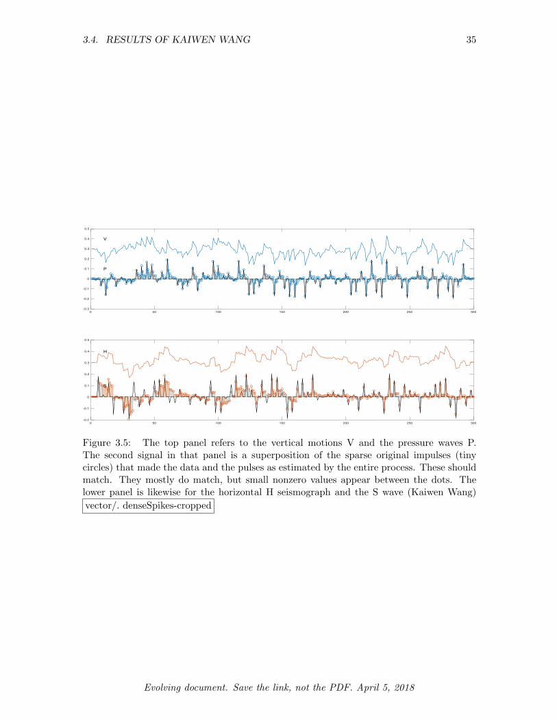
3.4. RESULTS OF KAIWEN WANG 35
0 50 100 150 200 250 300-0.3
-0.2
-0.1
0
0.1
0.2
0.3
0.4
0.5
V
P
0 50 100 150 200 250 300-0.2
-0.1
0
0.1
0.2
0.3
0.4
0.5
H
S
Figure 3.5: The top panel refers to the vertical motions V and the pressure waves P.The second signal in that panel is a superposition of the sparse original impulses (tinycircles) that made the data and the pulses as estimated by the entire process. These shouldmatch. They mostly do match, but small nonzero values appear between the dots. Thelower panel is likewise for the horizontal H seismograph and the S wave (Kaiwen Wang)vector/. denseSpikes-cropped
Evolving document. Save the link, not the PDF. April 5, 2018
36 CHAPTER 3. VECTOR-VALUED SIGNALS
Evolving document. Save the link, not the PDF. April 5, 2018

Chapter 4
Fitting while whitening residuals
First, we move to the world of Physics—operators far from convolution. Then we move morecompletely into the world of Geophysics—where often data is not on the uniform grid thatall PEFs demand. Naturally, we much prefer data on a uniform grid, but practicalities,especially land access, often prevent it. Science and engineering need the PEFs becausePEFs provide an essential statistical tool (IID) for fitting data to models. Indeed, PEFedresiduals sharply expose the mismatch between theory and observation. This mismatch iswhere discoveries often come to be made.
4.1 UPDATING MODELS WHILE UPDATING THE PEF
The basic data modeling problem takes the form: 0 ⇡ r(m) = A (Fm�d). For the specialcase m = 0, this regression is none other than the PEF problem that we solved in earlierchapters. The energy E in the residual r(m) is expressed as:
E = r · r = r⇤ r = (m⇤F⇤ � d⇤)A⇤A(Fm� d)). (4.1)
The model update direction is the negative of the energy gradient.
��m =@E
@m⇤ = F⇤A⇤A(Fm� d) = F⇤A⇤Ar. (4.2)
So, the new problem is to apply A⇤A to the residual r simultaneously with finding thePEF, A. Following are the steps to update the model grid:
y = (Fm� d) (4.3)r = A(Fm� d) = A y (4.4)q = A⇤A(Fm� d) = A⇤r = A⇤Ay (4.5)
��m = F⇤A⇤A(Fm� d) = F⇤q (4.6)
Equations above are in code below for computing q = A⇤Ay. Altogether, the tasks are:(1) to make y, (2) to estimate and apply A, (3) to apply A⇤, (4) to apply F⇤ getting �m,(5) to update the model m. Herein is code for simultaneusly finding A and for applyingA⇤A. Because F is yours, the rest is your job.
37
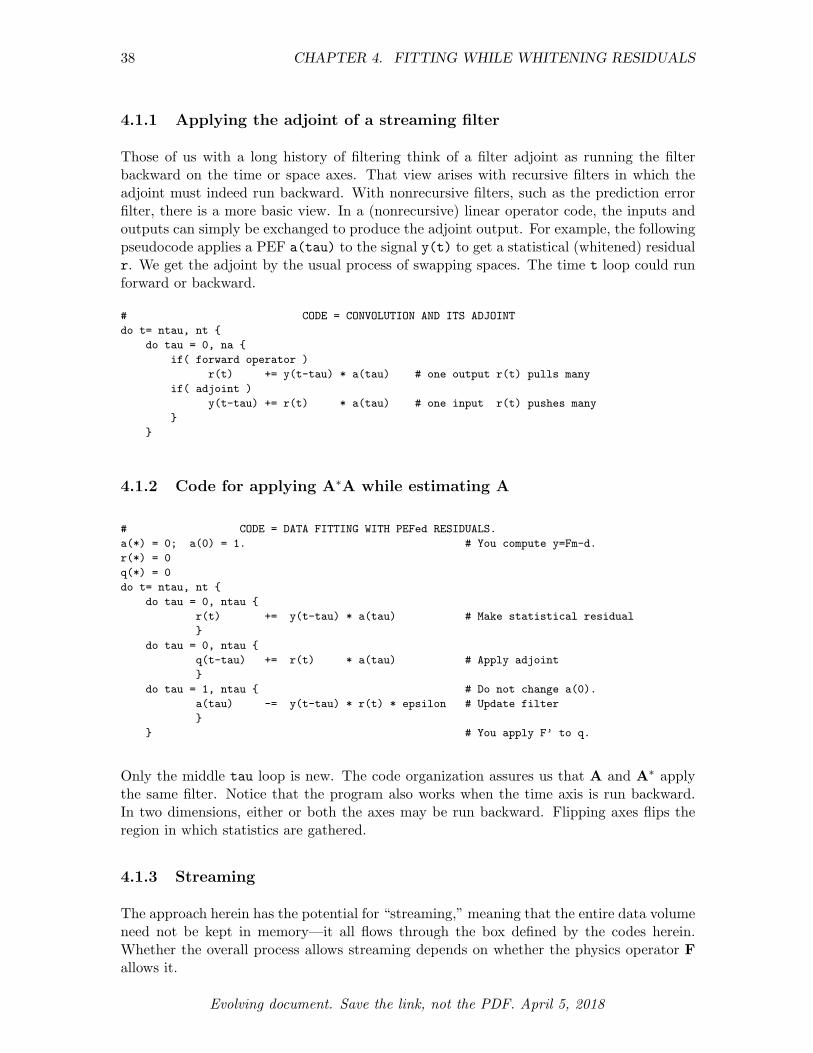
38 CHAPTER 4. FITTING WHILE WHITENING RESIDUALS
4.1.1 Applying the adjoint of a streaming filter
Those of us with a long history of filtering think of a filter adjoint as running the filterbackward on the time or space axes. That view arises with recursive filters in which theadjoint must indeed run backward. With nonrecursive filters, such as the prediction errorfilter, there is a more basic view. In a (nonrecursive) linear operator code, the inputs andoutputs can simply be exchanged to produce the adjoint output. For example, the followingpseudocode applies a PEF a(tau) to the signal y(t) to get a statistical (whitened) residualr. We get the adjoint by the usual process of swapping spaces. The time t loop could runforward or backward.
# CODE = CONVOLUTION AND ITS ADJOINTdo t= ntau, nt {
do tau = 0, na {if( forward operator )
r(t) += y(t-tau) * a(tau) # one output r(t) pulls manyif( adjoint )
y(t-tau) += r(t) * a(tau) # one input r(t) pushes many}
}
4.1.2 Code for applying A⇤A while estimating A
# CODE = DATA FITTING WITH PEFed RESIDUALS.a(*) = 0; a(0) = 1. # You compute y=Fm-d.r(*) = 0q(*) = 0do t= ntau, nt {
do tau = 0, ntau {r(t) += y(t-tau) * a(tau) # Make statistical residual}
do tau = 0, ntau {q(t-tau) += r(t) * a(tau) # Apply adjoint}
do tau = 1, ntau { # Do not change a(0).a(tau) -= y(t-tau) * r(t) * epsilon # Update filter}
} # You apply F’ to q.
Only the middle tau loop is new. The code organization assures us that A and A⇤ applythe same filter. Notice that the program also works when the time axis is run backward.In two dimensions, either or both the axes may be run backward. Flipping axes flips theregion in which statistics are gathered.
4.1.3 Streaming
The approach herein has the potential for “streaming,” meaning that the entire data volumeneed not be kept in memory—it all flows through the box defined by the codes herein.Whether the overall process allows streaming depends on whether the physics operator Fallows it.
Evolving document. Save the link, not the PDF. April 5, 2018

4.2. REGRIDDING: INVERSE INTERPOLATION OF SIGNALS 39
4.2 REGRIDDING: INVERSE INTERPOLATION OF SIGNALS
Figure 4.1 illustrates a universal problem in Geophysics and in many other fields. We wisha uniform mesh on the Earth surface from which linear interpolation would give our rawdata sprinkled on the surface. (Reflection seismology—using physics and math—explainsthe tranformation t! z).
Figure 4.1: Please, pretty please,build me a dense uniform mesh onthe Earth surface (x, y) plane. Fromthat mesh, I want to draw the datasprinkled in the (x, y) plane. Thosetwo gray boxes must be magic PEFs.The one in the (x, t) plane must goeverywhere on y2, then on y3, tocover the whole box. The other PEF,sweeps the volume perpendicularly.uniform/. WorldOfSignals
To achieve IID estimation, we can always use PEFs on model space (since we define it),but we often wish likewise for data space where PEFs could fill data gaps. Our goal hereis to make pseudo data on a uniform grid from the real data sprinkled about. Since this isan inversion problem, the pseudo data is the model space. The model m is located at xi =x0 + i�x, namely x=x0+ix*dx. Components of the observed signal data d each have withthem a location xd, namely xx(id)—likewise for 2-D space (x,y). Generally, the pseudodata m is gridded into somewhat more locations than the real data d so regularization isessential.
The 1-D linear operator L is defined by the following code. (2-D is similar.) Codeelements dd and mm are 1-D arrays of signals.
# CODE = LINEAR INTERPOLATION OF 1-D SIGNALSinteger 0 <= d <= nd # nd data signalsinteger 0 <= m <= nm # nm grid locationsreal mm(m) # components of mm are signals on a uniform gridreal dd(d) # components of dd are signals, recorded data.real xx(d) # locations of dd signal raw data recordings.real ox, dx # origin and delta of x grid coordinates.
do d = 0, nd # Data scan over all recorded signals.x = (xx(d)-x0)/dx # the value x points within the grid.ix = integer(x) # the value ix points to a place on the grid.if ( 0<ix< nm-1 ) # include only data signals inside the grid
f = x-ix # 0<f<1. closeness to ix+1g = 1.-f # 0<g<1. closeness to ix f+g=1.do t = 0, nt # Both dd and mm are functions of time.
if forwarddd(d) += ( g * mm(ix) + f * mm(ix+1))
else adjointmm(ix) += g * dd(d)mm(ix+1) += f * dd(d)
Evolving document. Save the link, not the PDF. April 5, 2018

40 CHAPTER 4. FITTING WHILE WHITENING RESIDUALS
Geophysics requires data, most often acquired on land (although also often at sea or inspace). On land it is often di�cult or impossible to acquire data on a regular grid, becausewe have limited access to land. But, mathematical algorithms are normally expressed ina form requiring a regular grid. And, PEFs require a uniform Cartesian grid. And more,PEFs are the only easy, large scale method of achieving IID. (Singular-value decompositionis much slower, suitable only for much smaller problems.) Resolving the data/theory gridconflict requires a process to synthesize pseudo data on a regular grid, from the given signalson a non regular grid. Such processes are a class of “inverse problems.”
4.2.1 Sprinkled signals go to a uniform grid via PEFed residuals
Sprinkled signals d means at arbitrary (xi, yi) lies your ith signal d = di,t. Herein wemake synthetic signals m = mt(x0 + j�x, y0 + k�y). The algorithm for building m is thefollowing:
1: Background2: m1 = Random trial model3: d1 = Lm1 trial data4: m2 = L⇤ d1 first guess model5: m3 = ↵m2 second guess, but ↵ unknown6: r = m1 �m3 test model residual7: r = m1 � ↵m2 test model residual, but ↵ unknown8: 0 = d(r · r)/d↵9: 0 = m2 · (m1 � ↵m2)10: ↵ = (m2 · m1)/(m2 · m2) ↵ is now a known property of L.
11: Initialization12: m = ↵L⇤ d estimated m assuming ↵,L⇤ and raw data d13: d = Lm estimated data14: r = d � d residual is raw minus estimated data15: r = d � Lm Given any m, this is the residual update rule.
16: Iteration17: r = d � Lm residual update rule18: m m + ✏dL⇤r use data to expand the model (fitting)19: m m � ✏mAm use PEF to shrink the model (regularizing)
It looks like we are ready to code. Since the iteration does not include ↵, I’m wonderingif we can simply ignore ↵. After verifying that ↵ is unit free, in the initialization we maysimply set ↵ = 1. It is worth a try.
Regularization being the flat-earth model
To simplify testing codes, we may use signals each consisting of a single scalar value. To seeenergy spreading out from a signal to surrounding model space locations, take the PEF Ato be simply the space derivative dm/dx. We may call dm/dx ⇡ 0 the “flat-earth” fitting
Evolving document. Save the link, not the PDF. April 5, 2018

4.2. REGRIDDING: INVERSE INTERPOLATION OF SIGNALS 41
goal.
r d � Lm (4.7)
m m + ✏d L⇤ r � ✏md
dxm (4.8)
Once the preceeding code works on scalar valued signals, we can upgrade to signalduration longer than a single scalar value. Signals would be placed somewhat randomlyalong a 1-D line on the earth surface. The test data d might be dipping layers. Some layerswould be thin (short on the time axis) others fat; some steeply dipping, some gentle. Onm space, fat gentle bedding should interpolate smoothly and continuously in space. Thinsteep bedding would break up into a series of fattened dots.
Learning the PEF while using it to interpolate
Going beyond the flat-earth assumption, let us interpolate a seismic receiver line. The wavearrival slope changes with time and space. Waves of di↵ering slopes and di↵ering frequenciesoften arrive at the same time. We need local PEFs to handle these complications occurringall together. Think of this:
m m + ✏d L⇤ r � ✏m Am (4.9)
Consider the e↵ect of the two terms, L⇤r and Am. First, r is the raw data minus the dataour model predicts. If our model m is too weak, its predicted data will be too weak, so theterm L⇤r will push more raw data into m.
Second, Am. It is learning A and trying to remove something from m. If we would setout to minimize Am without any restraints on m, then m would tend to zero. But herein,the +L⇤r supports m. What happens is that the PEF A bases itself on the well supportedlocations of m, getting a spectrum tending to the inverse to that of m. Where there areholes or weakly supported locations in m, they should tend to fill with a spectrum inverseto the PEF, namely the same spectrum as the well-supported aspects of m. Marvelous, eh?
I suggest the PEF estimation be done in a subroutine where the residual r is keptinternal, so not to be confused with the present residual r going into L⇤.
In chapters 1 and 2 the signal y was given everywhere with occasional exceptions forsome gaps. This suggests obtaining separately both A and m from their product Am mightbe impossible. However, here we likely have the data d guiding m rather tightly.
Take data organized somewhat like the model space, but with a substantial gap of miss-ing signals in it. Enough iterations of (4.9) should eventually fill the gap, albeit somewhattediously. Stationary theory has a fast method of filling long gaps commonly known asrecursion or polynomial division. This method might be important for covering long gaps,such as at cable ends. But in most applications, we have more modest goals, such as datasampling irregularities and gaps the size of streamer separations. Moreover, the speed ofthe method herein might render itself irrelevant, even on larger gaps. Do not give muchcredence to synthetic data far from real data. My old Russian friend, Boris would say,“Don’t trust what you have not paid for.”
Evolving document. Save the link, not the PDF. April 5, 2018

42 CHAPTER 4. FITTING WHILE WHITENING RESIDUALS
3-D flat-earth regularization
For 3-D data, an (x, y)-plane of signals, we penalize slopes in both x and y with the followingiteration:
m m + ✏d L⇤ r � ✏m [d
dx
d
dy]"
II
#
m (4.10)
This iteration should fill gaps with best fitting local plane waves.
3-D locally constant dip regularization
For the first time now, we do that which is not easy to do by any other method. Use two2-D PEFs, A and B, one for the (t, x)-plane, the other for the (t, y)-plane. In principle, a10 ⇥ 2 PEF in the (t, x) plane, likewise for the (t, y)-plane, adapts to dipping planes. Inpractice, 10⇥3 might work better. This and longer filters on the space axes allow for severalplane wave angles appearing simultaneously on the time axis. The fitting iterations are:
m m + ✏d L⇤ r � ✏m [A B]"
II
#
m (4.11)
We have not discussed the double PEF estimation algorithm necessary in this circumstance.Well, I need to leave some fun examples for my readers to map out. Remember, both the2-D filters A and B, filter all the (x, t) and (y, t) planes in the 3-D (x, y, t) volume of m.
Seismologists (they work to map t ! z) who have lived for years in (x, t) space, uponarriving in (x, y, t) space find themselves in awe at how much di↵erent the world feels.Without me speculating more on why, (which I easily could), I feel users of Equation (4.9)will be amazed when they first encounter results of Equation (4.11). Compare a solitarypicture on your retina, to a radiologist swimming throughout your body with a PET scan.She can glide anywhere she likes, all the while viewing down, forward, and sideways.
4.2.2 Is the theory worthwhile?
Questions
1. Is the foregoing method of data infill worthwhile?
2. At each iteration, PEFs go one direction. Should they be going opposite ways onalternate iterations?
3. What are conventional methods of infill?
4. We could average nearby data signals weighted inversely with distance. What is wrongwith that?
5. When traces have dipping events on them, how should they be interpolated?
6. Near a growth fault various dips may be simultaneousl present. Does it work?
7. Does the new method act like dip or azimuthal moveout?
Evolving document. Save the link, not the PDF. April 5, 2018

4.2. REGRIDDING: INVERSE INTERPOLATION OF SIGNALS 43
8. On a very dense grid in model space, we could nearest neighbor the data, then some-thing...
Answers
I don’t know. I don’t know. I dunno. I dunno. I dunno. I dunno. I dunno. I dunno. Lookslike we are not going to find out, either.
4.2.3 Repairing the navigation
Occasionally, data location is inaccurate. Historically, we have often seen that. Todaynavigation is usually quite good, but not universally so. Multicomponent seismometersalong with a pressure gauge are called “nodes.” Nodes may be placed on the ocean bottomwith a Remote Operated Vehicle (ROV), or alternately with a maned underwater vehicle.The surface boat knows its location well enough, but it may not be very certain where thenode is. I’m willing to work on this problem, but not until after I find colleagues to workon it with me.
The Galilee data set in GIEE is an example of data that gave me good reason to doubtthe navigation. But, it is 1990 vintage data with pre-satellite navigation.
4.2.4 Daydreams
I like to daydream about equation (4.9) and its relationship to the land surface of the USA.Many kinds of geophysical recorders lay sparse and irregular on the ground, so the factor(Fm�d) seems central to our e↵orts. Of course we need to flatten the Earth sphere givingus to wonder whether PEF concepts are limited to Cartesian spaces. The land surfacem is somewhat smooth in the plains whereas rough in the mountains. Where m in theplains is very smooth, there A must turn out to be a powerful roughener. There can be theoccasional sharply defined texture in the plains, so we will want softclip(Am) in the plainsas much as in the mountains.
Have a look with Google Earth or satellite maps. In the Appalachians there is a patternto the mountains not found in the Rockies. Follow the track from Harrisburg, Pennsylvaniato Birmingham Alabama. Occasionally these rolling mountains are broken through byrivers. After the land, look at the bottom of the oceans.
Ocean bottoms are tough places to get data. Many kinds of data (and data gaps!) a↵ectthe images we are able to see of the ocean floor. Everywhere there are stories to be told,half geological, and half about data acquisition limitations. Awesome! Let your imaginationrun.
Evolving document. Save the link, not the PDF. April 5, 2018

44 CHAPTER 4. FITTING WHILE WHITENING RESIDUALS
Evolving document. Save the link, not the PDF. April 5, 2018

Chapter 5
Appendices
5.1 WHY PEFs HAVE WHITE OUTPUT
It is somewhat intuitive that 1-D PEFs have a white output, but it is really amazing that2-D PEFs tend to spectral whiteness in a 2-D space; yet, this whiteness is extensivelydemonstrated in GIEE (Claerbout, 2014), while it is simply introduced and proven herenow.
5.1.1 Why 1-D PEFs have white output
1The basic idea of least-squares fitting is that the residual is orthogonal to each of the fittingfunctions. Applied to the PEF, this idea means the output of the PEF is orthogonal tolagged inputs. The orthogonality applies only for lags in the past, because prediction knowsonly the past while it aims to the future. What we soon see herein is di↵erent; namely,the output is uncorrelated with itself (as opposed to the input) for lags in both directions;therefore, the autocorrelation of the output is a delta function and the output spectrum iswhite. Knowing the PEF and having output whiteness has many applications.
Let d be a vector with components containing a time function. Let Znd representshifting the components to delay the signal in d by n samples. The definition of a PEF isthat it minimizes ||r|| by adjusting filter coe�cients a⌧ . The PEF output is as follows:
r = d + a1Z1d + a2Z
2d + a3Z3d + · · · (5.1)
We set out to choose the best a⌧ by setting to zero the derivative of (r · r) by a⌧ . After thebest a⌧ are chosen, the residual is perpendicular to each of the fitting functions as follows:
0 =d
da⌧(r · r) (5.2)
0 = r · drda⌧
= r · Z⌧d for ⌧ > 0. (5.3)
Given that 0 = r · Z⌧d, we examine r · Z⌧r and see that it also vanishes. Using Equation(5.1), we have for any autocorrelation lag k > 0,
r · Zkr = r · (Zkd + a1Zk+1d + a2Z
k+2d + ...)1This subsection draws from Levin et al. (2013), and is also included in Claerbout (2014).
45
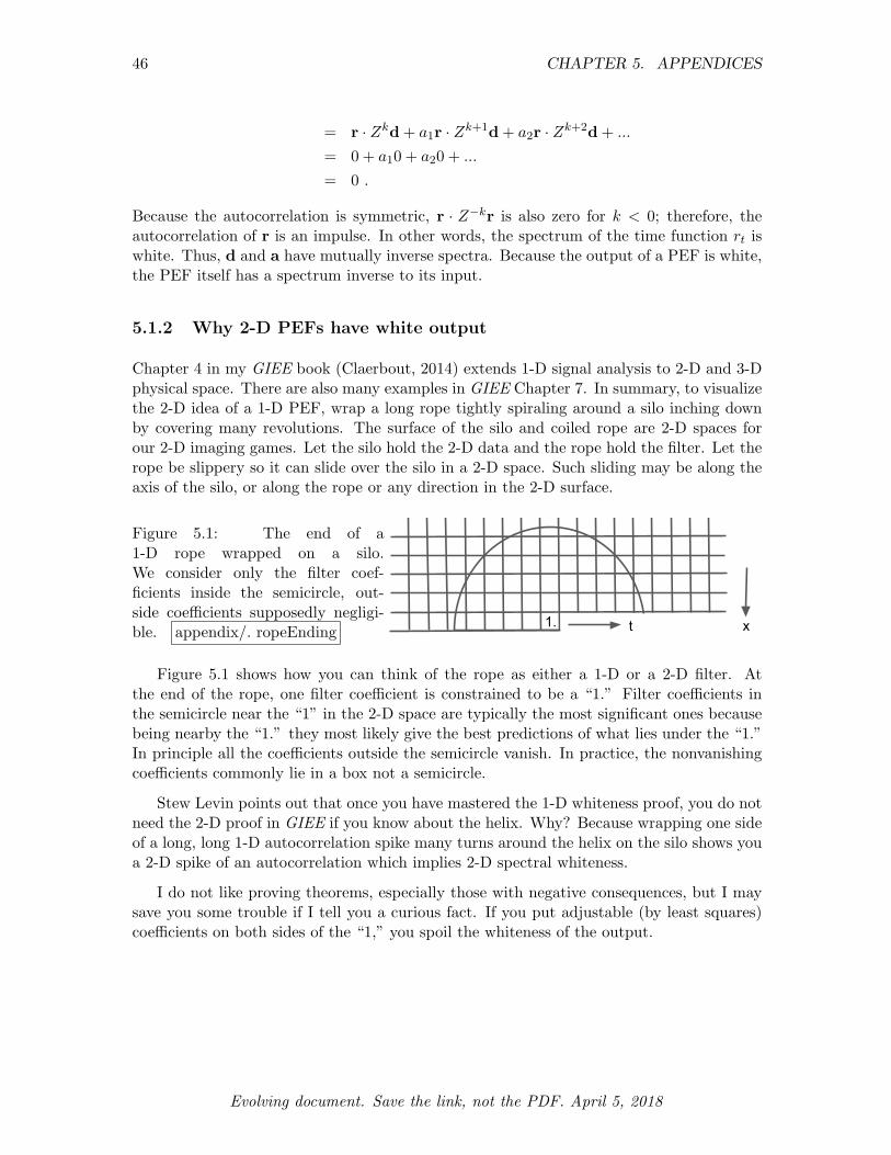
46 CHAPTER 5. APPENDICES
= r · Zkd + a1r · Zk+1d + a2r · Zk+2d + ...
= 0 + a10 + a20 + ...
= 0 .
Because the autocorrelation is symmetric, r · Z�kr is also zero for k < 0; therefore, theautocorrelation of r is an impulse. In other words, the spectrum of the time function rt iswhite. Thus, d and a have mutually inverse spectra. Because the output of a PEF is white,the PEF itself has a spectrum inverse to its input.
5.1.2 Why 2-D PEFs have white output
Chapter 4 in my GIEE book (Claerbout, 2014) extends 1-D signal analysis to 2-D and 3-Dphysical space. There are also many examples in GIEE Chapter 7. In summary, to visualizethe 2-D idea of a 1-D PEF, wrap a long rope tightly spiraling around a silo inching downby covering many revolutions. The surface of the silo and coiled rope are 2-D spaces forour 2-D imaging games. Let the silo hold the 2-D data and the rope hold the filter. Let therope be slippery so it can slide over the silo in a 2-D space. Such sliding may be along theaxis of the silo, or along the rope or any direction in the 2-D surface.
Figure 5.1: The end of a1-D rope wrapped on a silo.We consider only the filter coef-ficients inside the semicircle, out-side coe�cients supposedly negligi-ble. appendix/. ropeEnding
1. t x
Figure 5.1 shows how you can think of the rope as either a 1-D or a 2-D filter. Atthe end of the rope, one filter coe�cient is constrained to be a “1.” Filter coe�cients inthe semicircle near the “1” in the 2-D space are typically the most significant ones becausebeing nearby the “1.” they most likely give the best predictions of what lies under the “1.”In principle all the coe�cients outside the semicircle vanish. In practice, the nonvanishingcoe�cients commonly lie in a box not a semicircle.
Stew Levin points out that once you have mastered the 1-D whiteness proof, you do notneed the 2-D proof in GIEE if you know about the helix. Why? Because wrapping one sideof a long, long 1-D autocorrelation spike many turns around the helix on the silo shows youa 2-D spike of an autocorrelation which implies 2-D spectral whiteness.
I do not like proving theorems, especially those with negative consequences, but I maysave you some trouble if I tell you a curious fact. If you put adjustable (by least squares)coe�cients on both sides of the “1,” you spoil the whiteness of the output.
Evolving document. Save the link, not the PDF. April 5, 2018
5.2. THE HEART OF NONSTATIONARY PEF USING CALCULUS 47
5.2 THE HEART OF NONSTATIONARY PEF USING CALCULUS
2Suppose we have a PEF that represents all previous moments in time. Call it a =(1, a1, a2, a3, · · ·). Say that a represents the PEF (inverse spectrum) of the data values(d1, d2, d3, · · · , d98). We seek to define the a that represents the PEF with an appendeddata value d99. Consider the regression as follows:
2
666664
00000
3
777775⇡
2
666664
d99 d98 d97 d96
� · · ·· � · ·· · � ·· · · �
3
777775
2
6664
1a1
a2
a3
3
7775 � �
2
666664
01a1
a2
a3
3
777775(5.4)
The top row says we are trying to fit a new data point d99. The bottom block says thenew PEF a should be highly similar to the PEF that fit earlier data, a. The parameter �should be big enough that the new data point d99 does not change a very much. RewriteEquation (5.4) as follows:
2
6664
0000
3
7775 ⇡
2
6664
dn dn�1 dn�2
� 0 00 � 00 0 �
3
7775
2
64a1
a2
a3
3
75 �
2
6664
�dn+1
� a1
� a2
� a3
3
7775 (5.5)
or in a shortened block-matrix notation, we have the residual to minimize
0 ⇡ r ="
d⇤
� I
#
a �"�dn+1
� a
#
, (5.6)
where I is the identity matrix and
d =
2
64dn
dn�1
dn�2
3
75 , a =
2
64a1
a2
a3
3
75 ,
For decades Bernard “Bernie” Widrow (Wikipedia) attacked problems of this nature bydefining a quadratic form and finding its gradient. (Actually, he thinks in terms of circuitdiagrams.) Then he repeatedly made small steps down the gradient (not up). How big arethe small steps? Experience teaches.
The quadratic form is r⇤r. We take its derivative to find the search direction.
�a = � (some constant)@
@a⇤
����a=a
r⇤r (5.7)
Form the transpose of the Residual (5.6) and then, di↵erentiate by a⇤. (By a⇤, we meanthe complex conjugate transpose of a.)
@r⇤
@a⇤=
@
@a⇤{a⇤[d �I] � [�dn+1 �a]} = [d �I] (5.8)
2This section drawn on Fomel et al. (2016) and Claerbout (2017).
Evolving document. Save the link, not the PDF. April 5, 2018

48 CHAPTER 5. APPENDICES
and multiply that onto r from Equation (5.6) keeping in mind that d⇤a is a scalar.
�a / @r⇤
@a⇤r = [d �I]
("d⇤
� I
#
a �"�dn+1
� a
#)
(5.9)
= d(d⇤a) + �2a + ddn+1 � �2a (5.10)
�a / @r⇤
@a⇤
����a=a
r = (d⇤a + dn+1) d (5.11)
�a = � ✏ rt d (5.12)
It is certainly surprising that the analytic solution to the Regression (5.4) computationallyamounts to a single step of the optimization strategy (5.11), a strategy so crude as to beabsent from textbooks; yet true (Fomel et al., 2016). Experimentalists first notice thatEquation (5.4) demands we supply a not-given constant � while (1.3) or (5.12) demands anot-given constant ✏ (or �).
REFERENCES
Claerbout, J., 2014, Geophysical image estimation by example: Lulu.com.——–, 2017, Fitting while whitening nonstationary residuals: SEP-Report, 168, 255–262.Fomel, S., J. Claerbout, S. Levin, and R. Sarkar, 2016, Streaming nonstationary prediction
error (II): SEP-Report, 163, 271–277.Levin, S. A., J. Claerbout, and E. R. Martin, 2013, Shortest path to whiteness: SEP-Report,
150, 13–16.
Evolving document. Save the link, not the PDF. April 5, 2018