Nonstationary aspects of passive scalar gradient behaviour

European Journal of Mechanics B/Fluids 27 (2008) 433–443

Nonstationary aspects of passive scalar gradient behaviour

A. Garcia, M. Gonzalez ∗, P. Paranthoën

CNRS, UMR 6614, Laboratoire de Thermodynamique, CORIA, Site universitaire du Madrillet, 76801 Saint-Etienne du Rouvray, France

Received 25 May 2007; received in revised form 13 September 2007; accepted 13 September 2007

Available online 22 September 2007

Abstract

The dynamics of a passive scalar gradient experiencing fluctuating velocity gradient through the Lagrangian variations of strainpersistence is studied. To this end, a systematic, numerical analysis based on the equation for the orientation of the gradient ofa nondiffusive scalar in two-dimensional flow is performed. When the gradient responds weakly its orientation properties aredetermined by the mean value of strain persistence. Statistical alignment of the scalar gradient with the direction defined by theopposed actions of strain and rotation, by contrast, requires the gradient to keep up with strain persistence fluctuations. Theseresults have been obtained for both strain- and effective-rotation-dominated regimes and are supported by relevant experimentaldata. Consequences of the unsteady behaviour of the scalar gradient on mixing properties are also analysed.© 2007 Elsevier Masson SAS. All rights reserved.

PACS: 47.51.+a; 47.61.Ne; 47.27.-i

Keywords: Passive scalar gradient; Alignment properties; Mixing properties

1. Introduction

In random flows, in particular in chaotic or turbulent ones, the increase of the local, instantaneous gradient of ascalar such as temperature or concentration results in the enhancement of mixing through acceleration of moleculardiffusion. This “gradient production” is caused by the mechanical action of the velocity gradient, more precisely by itsstraining part, either in the pure straining motion of hyperbolic regions or in the vicinity of vortices where strain stemsfrom differential rotation. Quite equivalently, at least as far as only convective mechanisms are considered, hasteningof the mixing process in random flows finds expression in the stretching of material surface areas. In turbulent flowsthe growth of the scalar gradient is closely connected to the production of small scales of a scalar field and to cascadephenomena. Actually, the mean dissipation rate of the energy of fluctuations of a scalar is proportional to the varianceof its fluctuating gradient.

In the view where mixing properties of flows are explained through the evolution of the gradient of a scalar the keymechanisms rest on the alignment of the gradient with respect to the local strain principal axes [1–4]. The rise of thescalar gradient is indeed promoted by alignment with the most compressive direction of strain. But the general problemof scalar gradient alignment is quite complicated. In turbulent flows the question amounts to understanding how the

* Corresponding author.E-mail address: [email protected] (M. Gonzalez).

0997-7546/$ – see front matter © 2007 Elsevier Masson SAS. All rights reserved.doi:10.1016/j.euromechflu.2007.09.002

434 A. Garcia et al. / European Journal of Mechanics B/Fluids 27 (2008) 433–443

gradient behaves under the combined actions of molecular diffusion as well as of fluctuating strain and effectiverotation (i.e. vorticity plus strain basis rotation). In three-dimensional turbulence random alignment of vorticity andvorticity/strain interaction make the problem even more complex.

From pure kinematical considerations it is obvious that in incompressible flows the scalar gradient is drawn bythe local compressional direction. Yet it is also quite understandable that the latter is generally not the equilibriumorientation of the scalar gradient. In other words, when not only strain but also rotation and, possibly, moleculardiffusion are present, the fixed point of the gradient orientation equations is certainly not the strain compressional axis.In three-dimensional flows, the bare existence of this fixed point is even not proved in the general case [5]. In two-dimensional flows [6] as well as in a special, three-dimensional situation [7,8], however, the equilibrium orientationand conditions for its existence have been derived analytically at least when the scalar is nondiffusive. It has alsobeen shown that in two-dimensional turbulence the scalar gradient statistically aligns better with the local equilibriumdirection defined by the balance between strain and rotation than with the compressional direction [6].

Even so, the statistical alignment of the scalar gradient is determined by the gradient dynamics. If the velocity fieldis time varying, alignment with a possible equilibrium orientation requires that the response time scale of the scalargradient is short enough compared to the time scale of velocity gradient fluctuations. Alignment dynamics is thus anessential feature of the scalar gradient behaviour and has already been addressed in some studies [2,4,7,9–11]. Theinfluence on mixing that follows from this nonstationary aspect is still not clear.

Trying to understand how the mixing process is affected by the dynamics of the scalar gradient is precisely one ofthe main goals of the present study. This is done in Section 3 by analysing numerically the growth rate of the gradientnorm for different unsteady regimes in the two-dimensional case. We first devote Section 2 to the numerical analysisof alignment statistics when the scalar gradient undergoes a fluctuating strain persistence. This investigation aimsat bearing out the generality of the partial findings of Ref. [11]. In particular, the orientation equation of the scalargradient in a two-dimensional flow is solved for simulating the strain-dominated as well as the effective-rotation-dominated regimes. Different strain persistence signals are used to show the existence of a gradient alignment thatis neither the compressional nor the equilibrium direction defined by the instantaneous strain persistence. Section 4reports on experimental results supporting the latter numerical study. Conclusion is drawn in Section 5.

2. Analysis of statistical scalar gradient alignment

2.1. Equation for scalar gradient orientation

We restrict the analysis to two-dimensional, incompressible flow and nondiffusive passive scalar. Writing the scalargradient in the fixed frame of reference as G = |G|(cos θ, sin θ), the equation for the gradient orientation is [6,9]

dζ

dτ= r − cos ζ, (1)

where ζ = 2(θ +Φ) gives the gradient orientation in the local strain basis; angle Φ defines the orientation of the strainprincipal axes through tanΦ = σn/σs with σn = ∂u/∂x − ∂v/∂y and σs = ∂v/∂x + ∂u/∂y denoting the normal andshear components of strain, respectively. Time τ is a strain-normalised time

τ =t∫

0

σ(t ′) dt ′,

with t standing for the Lagrangian time and σ for strain intensity, σ 2 = σ 2n + σ 2

s .Note that Eq. (1) just proceeds from the usual equation for the passive scalar (with molecular diffusion neglected)

through the equation for the scalar gradient [4,7] which is handled as explained in Ref. [6].Parameter r represents the persistence of strain [6,12] and is defined as

r = ω + 2dΦ/dt

σ,

where ω = ∂v/∂x − ∂u/∂y is vorticity. Strain persistence, r , defines an objective criterion for partitioning the flow; instrain-dominated regions r2 < 1, while in regions where effective rotation prevails r2 > 1. In this article these regions

A. Garcia et al. / European Journal of Mechanics B/Fluids 27 (2008) 433–443 435

are occasionally termed hyperbolic and elliptic respectively. It is to be noticed that this partition does not necessarilycoincide with the one derived from the Okubo–Weiss criterion; because r includes the pressure Hessian through strainbasis rotation, dΦ/dt , the corresponding criterion is more general [13].

Lapeyre et al. [6] analysed Eq. (1) assuming slow variations of r along Lagrangian trajectories and showed the wayin which the scalar gradient orientation is determined by the local flow topology. For prevailing strain the orientationequation has a stable fixed point,

ζeq = − arccos(r),

which corresponds to an equilibrium orientation. In the special case r = 0 (i.e. in the pure hyperbolic regime) theequilibrium orientation, ζeq, coincides with the local compressional direction,

ζc = −π/2.

If effective rotation dominates, Eq. (1) has no fixed point; there is no equilibrium orientation for the scalar gradient,but a most probable one given by

ζprob = [1 − sign(r)

]π/2.

Exact balance between strain and effective rotation, namely r2 = 1, drives the scalar gradient to align with the bisectorof strain principal axes. The general solution, ζ(τ ), of Eq. (1) can be derived for any of the latter three differentregimes [6].

The study of Garcia et al. [11] reveals that the above approach remains valid as long as the response time scaleof the scalar gradient is short enough compared to the time scale of the Lagrangian fluctuations of r . They also putforward that in the opposite case, namely when the gradient does not keep up with r fluctuations and its responseis poor, the alignment of the scalar gradient is determined by the mean value of r , 〈r〉. In the following we try togeneralise and support these results by the study of regimes that have not been originally addressed. Indeed we extendthe previous analysis by examining the effective-rotation-dominated regime in addition to the strain-dominated one.Considering different values of 〈r〉 we also confirm the existence of the orientation defined by the mean value of strainpersistence.

2.2. Alignment of scalar gradient in the case of fluctuating strain persistence

We simulate the fluctuations of strain persistence, r , with a stochastic differential equation,

dr = −(r − 〈r〉)β� dτ + (2r ′2β� dτ)1/2ξ. (2)

In Eq. (2) ξ is a standardised Gaussian random variable. This equation depends on three parameters, namely β�,〈r〉 and r ′. Giving β� a value is equivalent to prescribe the nondimensional integral time scale of r , T �, throughT � = 1/β�. Parameter r ′ stands for the root mean square of r . The few data on strain persistence statistics [6,11]show it is not a Gaussian variable. However, the actual statistics are immaterial here, for the concern is mainly in thegradient response to time-varying strain persistence.

The evolution of the scalar gradient orientation, then, is derived by solving numerically

dζ = [r(τ ) − cos ζ

]dτ. (3)

Since dτ = σ dt , it is clear from Eq. (3) that the response time scale of the gradient orientation to the forcing mech-anism represented by r is of the order of 1/σ . Parameter β� gives a measure of the gradient response compared toforcing stimulation. Small values of β� (resp. slow variations of r) mean that the scalar gradient responds well to r

fluctuations, while large values (resp. fast variations of r) correspond to a poor response of the scalar gradient. In thespecial case for which strain intensity, σ , is constant β� = 1/σT where T is the integral time scale of r signal andthus β� is the ratio of gradient response time scale to r fluctuations time scale.

Garcia et al. [11] have shown that the approach of Lapeyre et al. [6] (Section 2.1) does not apply to scalar gradientorientation if strain persistence fluctuates too rapidly for the scalar gradient to respond. They argued that in this casethe most probable orientation of the gradient should be determined by the mean value of r , 〈r〉, rather than by theinstantaneous one. In particular, it was put forward that if 〈r〉2 < 1 (in other words, if the regime is hyperbolic on


Fig. 1. P.d.f’s of scalar gradient orientation for 〈r〉 = 0 and r ′2 = 4 conditioned on r2 < 1 (dominating strain). P.d.f of ζ − ζ〈r〉: " β� = 5,! β� = 0.01; p.d.f of ζ − ζeq: 2 β� = 5, 1 β� = 0.01.

Fig. 2. P.d.f’s of scalar gradient orientation for 〈r〉 = 0 and r ′2 = 4 conditioned on r2 > 1 (dominating effective rotation). P.d.f of ζ −ζ〈r〉: " β� = 5,! β� = 0.01; p.d.f of ζ − ζprob: 2 β� = 5, 1 β� = 0.01.

an average) and the time scale of r fluctuations is shorter than the gradient response time scale, the preferentialorientation of the gradient should be defined by

ζ〈r〉 = − arccos〈r〉.In reality, the most probable orientation cannot be determined analytically, but is close to ζ〈r〉. This results from the factthat the weaker the gradient response, the closer ζ to ζ〈r〉. A simplified proof is given in Appendix A. The behaviour ofthe scalar gradient when its response to r fluctuations is poor is confirmed by the present simulations for two differentvalues of 〈r〉 as well as for small and large values of β�.

The p.d.f’s of scalar gradient alignment have been derived from the numerical evolution of ζ computed usingEqs. (3) and (2) with 〈r〉 = 0 and r ′2 = 4. The fluctuations of r thus describe the hyperbolic regime (r2 < 1), but alsomake significant inroads into the elliptic one (r2 > 1). The p.d.f’s of ζ − ζeq and ζ − ζ〈r〉 conditioned on r2 < 1 areshown in Fig. 1. They indicate which of the orientations ζeq (determined by the instantaneous value of r ; Section 2.1)


Fig. 3. P.d.f’s of scalar gradient orientation for 〈r〉 = −0.8, r ′2 = 4 and β� = 100 conditioned on r2 < 1 (dominating strain). " p.d.f of ζ − ζ〈r〉;2 p.d.f of ζ − ζeq; × p.d.f of ζ − ζc.

Fig. 4. P.d.f’s of scalar gradient orientation for 〈r〉 = −0.8, r ′2 = 4 and β� = 100 conditioned on r2 > 1 (dominating effective rotation). " p.d.f ofζ − ζ〈r〉; 2 p.d.f of ζ − ζprob; × p.d.f of ζ − ζc.

and ζ〈r〉 (defined by 〈r〉) is statistically the best one in the hyperbolic regime. Clearly, for β� = 0.01 the scalar gradientpreferentially aligns with the instantaneous, equilibrium direction, ζeq, which is generally different from the compres-sion one, in agreement with the approach by Lapeyre et al. [6]. For β� = 5 it is the alignment with the direction definedby ζ〈r〉 which is the most probable one. Note that for 〈r〉 = 0 ζ〈r〉 = −π/2 and thus coincides with the compressionaldirection. Interestingly, in the present case the scalar gradient thus statistically aligns with the compressional direc-tion because the gradient response to r fluctuations is poor (β� > 1) and the mean value of r corresponds to a purehyperbolic regime (〈r〉 = 0). This is reminiscent of the experimental situation analysed by Garcia et al. [11].

The results in the elliptic regime (p.d.f’s conditioned on r2 > 1; Fig. 2) are similar. For β� = 0.01 the most probablegradient orientation is given by ζprob (Section 2.1) which agrees with the analysis of Lapeyre et al. [6]. In the caseβ� = 5 the scalar gradient again aligns preferentially with the direction defined by ζ〈r〉, that is, the compressionalone. Yet this is not paradoxical. When the scalar gradient does not respond to the fluctuations of r its orientation is


governed by the mean value, 〈r〉, rather than by the instantaneous one and remains close to ζ〈r〉. This may drive thegradient to align with the compressional direction, even though r takes elliptic values, provided that 〈r〉 is close tozero. Note that the secondary maxima in Fig. 2 are explained by |ζ〈r〉 − ζprob| = |ζc − ζprob| = π/2.

Alignment p.d.f’s derived with 〈r〉 = −0.8 are plotted in Figs. 3 and 4. If β� is small the value of 〈r〉 is immaterial;the scalar gradient preferentially aligns with the equilibrium direction, ζeq, and the same orientation p.d.f’s as thoseplotted in Figs. 1 and 2 for β� = 0.01 are derived. Figs. 3 and 4 thus only display the orientation p.d.f’s in the casewhere β� is given a large value, β� = 100. Results for the hyperbolic regime are presented in Fig. 3. Plainly, ζ〈r〉(which is computed as ζ〈r〉 = − arccos(−0.8)) is the most probable orientation of the scalar gradient. Alignment withthe equilibrium direction, ζeq, is weak and as shown by the p.d.f of ζ − ζc there is no trend of the gradient to alignwith the compressional direction.

In the elliptic regime (Fig. 4), too, the orientation defined by 〈r〉 is statistically the best one. As a matter of course,the gradient does not align with the compressional direction, but there is also no trend at all toward the directiondefined by ζprob.

3. “Gradient production” and mixing properties

With the same assumptions as those stated in Section 2.1 the equation for the norm of the scalar gradient is [6,9]

2

|G|d|G|dτ

= − sin ζ,

from which it is clear that the mean growth rate of the gradient norm, ρ, is given by ρ = −〈sin ζ 〉. Note that alignmentwith the compressional direction, ζ = ζc = −π/2, corresponds to the maximum growth rate.

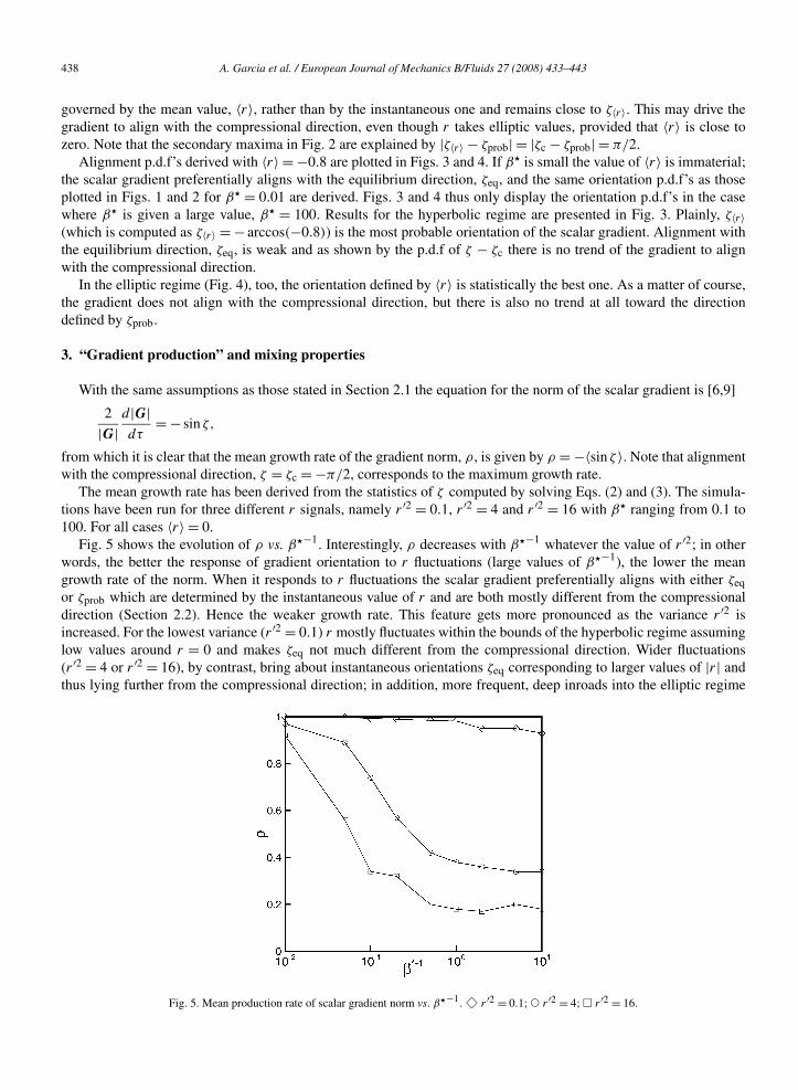
The mean growth rate has been derived from the statistics of ζ computed by solving Eqs. (2) and (3). The simula-tions have been run for three different r signals, namely r ′2 = 0.1, r ′2 = 4 and r ′2 = 16 with β� ranging from 0.1 to100. For all cases 〈r〉 = 0.

Fig. 5 shows the evolution of ρ vs. β�−1. Interestingly, ρ decreases with β�−1 whatever the value of r ′2; in otherwords, the better the response of gradient orientation to r fluctuations (large values of β�−1), the lower the meangrowth rate of the norm. When it responds to r fluctuations the scalar gradient preferentially aligns with either ζeqor ζprob which are determined by the instantaneous value of r and are both mostly different from the compressionaldirection (Section 2.2). Hence the weaker growth rate. This feature gets more pronounced as the variance r ′2 isincreased. For the lowest variance (r ′2 = 0.1) r mostly fluctuates within the bounds of the hyperbolic regime assuminglow values around r = 0 and makes ζeq not much different from the compressional direction. Wider fluctuations(r ′2 = 4 or r ′2 = 16), by contrast, bring about instantaneous orientations ζeq corresponding to larger values of |r| andthus lying further from the compressional direction; in addition, more frequent, deep inroads into the elliptic regime

Fig. 5. Mean production rate of scalar gradient norm vs. β�−1. E r ′2 = 0.1; ! r ′2 = 4; 1 r ′2 = 16.


(r2 > 1) even lead the gradient to align with ζprob, that is, 45◦ away from the compressional direction, during longertime intervals. As a result, for moderate and large values of β�−1 the mean growth rate of the scalar gradient normis lowered as the amplitude of r fluctuations is increased. For the smallest values of β�−1, though, the growth rate isinsensitive to r variance and is close to its maximum value. Indeed a sluggish response to r fluctuations compels thegradient to remain aligned with the direction defined by 〈r〉 (Section 2.2) which in the present case (for which 〈r〉 = 0)coincides with the compressional direction.

There is an interesting consequence for mixing properties. If 〈r〉 � 0, then favourable conditions for mixing are notonly achieved in the hyperbolic regime; provided that the gradient response is weak, they are also fulfilled in thosecases where large fluctuations of r span both the hyperbolic and elliptic regimes. More generally, when r fluctuateswith 〈r〉 remaining close to 0 it is the poor response of the scalar gradient to r fluctuations that promotes the bestconditions for fast mixing.

4. Analysis of experimental data on scalar gradient alignment

As far as we know, simultaneous measurements of velocity and scalar gradients are scarce. Apart from experi-ments in turbulent flows [14], joint statistics of velocity gradient and temperature gradient have been measured ina low-Reynolds number, two-dimensional, Bénard–von Kármán street [15,16]. The latter data confirm that for fastfluctuations of strain persistence the preferential orientation of the scalar gradient is determined by the mean strainpersistence rather than by its instantaneous value.

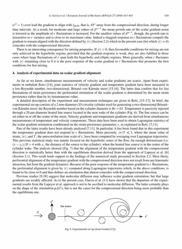
A detailed description of the experiment and measurement techniques are given in Refs. [15–17]. In brief, theexperimental set-up consists of a 2 mm-diameter (D) circular cylinder used for generating a two-dimensional Bénard–von Kármán street; the Reynolds number based on the cylinder diameter is Re = 63. Temperature is passively injectedthrough a 20 µm-diameter heated line source located in the near wake of the cylinder (Fig. 6). The line source can beset either in or off the centre of the street. Velocity gradients and temperature gradients are derived from simultaneousmeasurements of temperature and velocity components. These data have been used to obtain Lagrangian statistics ofthe scalar gradient orientation conditioned on the strain persistence parameter, r , as explained in Refs. [7,11].

Part of the latter results have been already analysed [7,11]. In particular, it has been found that in this experimentthe temperature gradient does not respond to r fluctuations. More precisely, 〈σ 〉T � 1, where the mean value ofstrain, 〈σ 〉, and T , the autocorrelation time scale of r , have been computed by averaging over Lagrangian trajectories.This previous statistical study was mainly focused on the hyperbolic zones of the flow, far enough downstream (i.e.(x − xs)/D > 4 with xs the distance of the source to the cylinder), when the heated line source is in the centre of thecylinder wake. The analysis showed (Fig. 7) that the alignment of the temperature gradient with the compressionaldirection is statistically better than with the equilibrium direction derived from the approach of Lapeyre et al. [6](Section 2.1). This result lends support to the findings of the numerical study presented in Section 2.2. Most likely,preferential alignment of the temperature gradient with the compressional direction does not result from any kinematicattraction, but from the gradient dynamics. Because of the poor response of the temperature gradient to r fluctuations,the preferential alignment is given by 〈r〉 computed along Lagrangian trajectories which, in the above conditions, isfound to be close to 0 and thus defines an orientation that almost coincides with the compressional direction.

Previous studies [9,18] suggest that molecular diffusion may influence scalar gradient orientation, but that largegradients are weakly affected. As to the present case, Garcia et al. [11] have shown that the departure of the experi-mental results from the Lapeyre et al. approach is not to be ascribed to molecular diffusion. The latter certainly playson the shape of the orientation p.d.f’s, but is not the cause for the compressional direction being more probable thanthe equilibrium one.

Fig. 6. Experimental set-up (from Godard [15]).


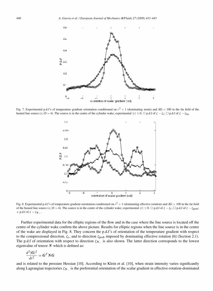
Fig. 7. Experimental p.d.f’s of temperature gradient orientation conditioned on r2 < 1 (dominating strain) and |G| > 100 in the far field of theheated line source (x/D > 4). The source is in the centre of the cylinder wake; experimental 〈r〉 � 0. ! p.d.f of ζ − ζc; 1 p.d.f of ζ − ζeq.

Fig. 8. Experimental p.d.f’s of temperature gradient orientation conditioned on r2 > 1 (dominating effective rotation) and |G| > 100 in the far fieldof the heated line source (x/D > 4). The source is in the centre of the cylinder wake; experimental 〈r〉 � 0. ! p.d.f of ζ − ζc; 1 p.d.f of ζ − ζprob;× p.d.f of ζ − ζN− .

Further experimental data for the elliptic regions of the flow and in the case where the line source is located off thecentre of the cylinder wake confirm the above picture. Results for elliptic regions when the line source is in the centreof the wake are displayed in Fig. 8. They concern the p.d.f’s of orientation of the temperature gradient with respectto the compressional direction, ζc, and to direction ζprob imposed by dominating effective rotation [6] (Section 2.1).The p.d.f of orientation with respect to direction ζN− is also shown. The latter direction corresponds to the lowesteigenvalue of tensor N which is defined as:

d2|G|2dt2

= GT NG

and is related to the pressure Hessian [10]. According to Klein et al. [10], when strain intensity varies significantlyalong Lagrangian trajectories ζN− is the preferential orientation of the scalar gradient in effective-rotation-dominated


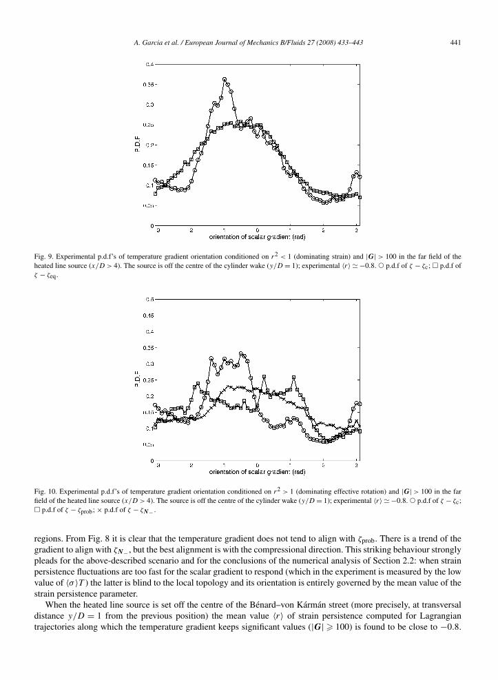
Fig. 9. Experimental p.d.f’s of temperature gradient orientation conditioned on r2 < 1 (dominating strain) and |G| > 100 in the far field of theheated line source (x/D > 4). The source is off the centre of the cylinder wake (y/D = 1); experimental 〈r〉 � −0.8. ! p.d.f of ζ − ζc; 1 p.d.f ofζ − ζeq.

Fig. 10. Experimental p.d.f’s of temperature gradient orientation conditioned on r2 > 1 (dominating effective rotation) and |G| > 100 in the farfield of the heated line source (x/D > 4). The source is off the centre of the cylinder wake (y/D = 1); experimental 〈r〉 � −0.8. ! p.d.f of ζ − ζc;1 p.d.f of ζ − ζprob; × p.d.f of ζ − ζN− .

regions. From Fig. 8 it is clear that the temperature gradient does not tend to align with ζprob. There is a trend of thegradient to align with ζN− , but the best alignment is with the compressional direction. This striking behaviour stronglypleads for the above-described scenario and for the conclusions of the numerical analysis of Section 2.2: when strainpersistence fluctuations are too fast for the scalar gradient to respond (which in the experiment is measured by the lowvalue of 〈σ 〉T ) the latter is blind to the local topology and its orientation is entirely governed by the mean value of thestrain persistence parameter.

When the heated line source is set off the centre of the Bénard–von Kármán street (more precisely, at transversaldistance y/D = 1 from the previous position) the mean value 〈r〉 of strain persistence computed for Lagrangiantrajectories along which the temperature gradient keeps significant values (|G| � 100) is found to be close to −0.8.


Fig. 9 shows the p.d.f’s of temperature gradient orientation with respect to either the compressional direction or theequilibrium direction, ζeq, derived from the approach of Lapeyre et al. [6], in strain-dominated regions. There is a trendof the gradient to align with ζeq. However, a much better statistical alignment is found with the direction correspondingto ζ − ζc � −1, that is, with ζ � −1 − π/2 � − arccos(−0.8) = − arccos〈r〉. P.d.f’s of Fig. 9 are more distributedand thus display lower peaks than those corresponding to the source being in the centre of the cylinder wake (Fig. 7).This may result from a bigger influence of rotation on the temperature gradient when the line source is off the centreof the wake. Orientation statistics in effective-rotation-dominated regions have similar trends. Fig. 10 shows that thetemperature gradient aligns slightly better with ζN− than with ζprob. But in this case, too, the best statistical alignment– broader though the p.d.f is – is found around ζ � − arccos(−0.8). These latter experimental data with 〈r〉 = 0 thusgive a more general support to the previous findings on the dynamics of scalar gradient orientation.

5. Conclusion

Analysis of the behaviour of the passive scalar gradient undergoing the influence of varying velocity derivativesthrough fluctuating strain persistence uncovers some interesting results regarding both the statistical gradient orienta-tion and mixing properties.

Generalising the analysis of Garcia et al. [11] to the effective-rotation-dominated regime, we confirm that the statis-tics of scalar gradient alignment depend on the gradient response to strain persistence fluctuations. More precisely, thenumerical study based on the equation for the scalar gradient orientation in two-dimensional flow shows that perfectresponse drives the gradient to preferentially align with a direction determined by the instantaneous value of strainpersistence as predicted by the analysis of Lapeyre et al. [6]. When the response of the scalar gradient is poor, though,the preferential alignment is given by the mean value of strain persistence which indicates whether the flow regimeis, on an average, either strain- or effective-rotation-dominated. It follows interestingly that the scalar gradient prefer-entially aligns with the compressional direction provided that it is almost insensitive to strain persistence fluctuationsand the mean strain persistence is close to the pure hyperbolic value. This result opposes the usual statement that it isa perfect response to the fluctuating rotation of the strain basis (which in the two-dimensional case is explicit in thestrain persistence parameter) that leads the gradient to align with the compressional direction.

The general picture derived from the numerical study is firmly supported by experimental, Lagrangian joint statis-tics of velocity gradient and scalar gradient derived from simultaneous measurements of velocity and temperature in atwo-dimensional, low-Reynolds number Bénard–von Kárman street. It is worth noting that its low Reynolds numbermarks this flow from the simulated two-dimensional turbulent flows in which scalar gradient alignment was previ-ously studied [6,9]. In particular, it may be that alignment with the equilibrium direction found by Lapeyre et al. [6]results from a good response of the scalar gradient to r fluctuations in turbulent flows (moderate or large σT ). Check-ing this surmise would require Lagrangian data on strain persistence in two-dimensional turbulence. Regarding theLagrangian properties of strain persistence and scalar gradient dynamics, another interesting and unanswered issue iswhether the present flow is a special one or belongs to a more general class of flows.

Finally, unsteady behaviour of the scalar gradient may unexpectably affect mixing properties through alignmentstatistics. An interesting result is that poor response of the gradient to strain persistence fluctuations does not inevitablyoppose efficient mixing. In particular, the study of the growth rate of the gradient norm clearly shows that when themean strain persistence is close to the pure hyperbolic value (in other words, strain is persistent on an average) it isthe weak response of the gradient to strain persistence fluctuations which promotes the highest growth rate and thusthe best conditions for mixing.

Appendix A. Behaviour of scalar gradient orientation for fast fluctuations of strain persistence

We restrict to the case where 〈r〉2 < 1 and ζ〈r〉 = − arccos〈r〉 is defined.From Eq. (1) the equation for the difference ζ � = ζ − ζ〈r〉 is:

dζ �

dτ= r − 〈r〉 cos ζ � − γ sin ζ � (A.1)

with τ = ∫ tσ (t ′) dt ′ and γ = (1 − 〈r〉2)

1/2.
0


We get rid of the nonlinearity of Eq. (A.1) by assuming small values of ζ �. To first order, then:

dζ �

dτ+ γ ζ � = r ′ (A.2)

with r ′ = r − 〈r〉. The proof is thus not general, but is given as an additional argument for the behaviour of the scalargradient when its response to r fluctuations is poor.

We assume a sine signal for r ′, r ′ = a sinω�τ , in which frequency is normalised as ω� = ω/〈σ 〉 with 〈σ 〉 = τ/t .The nondimensional frequency, ω�, thus gives a measure of the response of the scalar gradient to r fluctuations. Inparticular, poor response is expected for large values of ω�.

The solution of Eq. (A.2) is:

ζ � =[ζ �(0) + aω�

ω�2 + γ 2

]exp(−γ τ) + a

γ (1 + ω�2/γ 2)

(sinω∗τ − ω�

γcosω�τ

). (A.3)

Note that Eq. (A.3) can be recast in the more standard form:

ζ � =[ζ �(0) + aω�

ω�2 + γ 2

]exp(−γ τ) + a

γ (1 + ω�2/γ 2)1/2

sin(ω�τ − φ)

with cosφ = (1 + ω�2/γ 2)−1/2

and phase, φ, is present when the response to the stimulation is not perfect.From Eq. (A.3) the long-time evolution of ζ � is given by:

ζ � � a

γ (1 + ω�2/γ 2)


γcosω�τ

).

For ω� 1:

ζ � � a

ω�2/γ


γcosω�τ

).

Since ω�/γ 1, ζ � is bounded as:

− a

ω�� ζ � � a

ω�.

It follows that when r fluctuates on a much shorter time scale than the response time scale of the scalar gradient somuch so that the latter does not keep up with r fluctuations the gradient orientation, ζ , remains close to ζ〈r〉. Increasingthe amplitude of r fluctuations, however, leads to the opposite behaviour.

References

[1] A. Pumir, Phys. Fluids 6 (1994) 2118.[2] W.D. Smyth, J. Fluid Mech. 401 (1999) 209.[3] P. Vedula, P.K. Yeung, R.O. Fox, J. Fluid Mech. 433 (2001) 29.[4] G. Brethouwer, J.C.R. Hunt, F.T.M. Nieuwstadt, J. Fluid Mech. 474 (2003) 193.[5] M. Tabor, I. Klapper, Chaos Solitons Fractals 4 (1994) 1031.[6] G. Lapeyre, P. Klein, B.L. Hua, Phys. Fluids 11 (1999) 3729.[7] A. Garcia, Ph.D. thesis, University of Rouen, 2006.[8] A. Garcia, M. Gonzalez, Phys. Fluids 18 (2006) 058101.[9] G. Lapeyre, B.L. Hua, P. Klein, Phys. Fluids 13 (2001) 251.

[10] P. Klein, B.L. Hua, G. Lapeyre, Physica D 146 (2000) 246.[11] A. Garcia, M. Gonzalez, P. Paranthoën, Phys. Fluids 17 (2005) 117102.[12] E. Dresselhaus, M. Tabor, J. Fluid Mech. 236 (1991) 415.[13] B.L. Hua, P. Klein, Physica D 113 (1998) 98.[14] B. Galanti, G. Gulitsky, M. Kholmyansky, A. Tsinober, S. Yorish, in: H.I. Andersson, P.-Å. Krogstad (Eds.), Advances in Turbulence X,

Proceedings of the 10th European Turbulence Conference, Trondheim, Norway, 2004.[15] G. Godard, Ph.D. thesis, University of Rouen, 2001.[16] G. Godard, M. Gonzalez, P. Paranthoën, in: I.P. Castro, P.E. Hancock, T.G. Thomas (Eds.), Advances in Turbulence IX, Proceedings of the

9th European Turbulence Conference, Southampton, United Kingdom, 2002.[17] P. Paranthoën, G. Godard, F. Weiss, M. Gonzalez, Int. J. Heat Mass Transfer 47 (2004) 819.[18] P. Constantin, I. Procaccia, D. Segel, Phys. Rev. E 51 (1995) 3207.

Nonstationary aspects of passive scalar gradient behaviour

Documents

Transcript of Nonstationary aspects of passive scalar gradient behaviour