NONPARALLEL YIELD CURVE SHIFTS AND CONVEXITY ROBERT R. REITANO

TRANSACTIONS OF SOCIETY OF ACTUARIES 1992 VOL, 44

NONPARALLEL YIELD CURVE SHIFTS AND CONVEXITY

ROBERT R. REITANO

ABSTRACT

The conventional wisdom about convexity is that positive convexity is good, and more is better. Paradoxically, while defensible in theory, this maxim has been found to fail in practice. In this paper, the relationship of convexity to the assumption of parallel shifts is explored, and new convexity measures are developed to reflect nonparallel shifts. These new measures can differ dramatically from the traditional values, providing insight into when convexity does not have to be good and when it does.

1. INTRODUCTION

It is generally assumed that positive convexity is good, and more convexity is better than less. However, actual performance studies do not necessarily bear out this conventional wisdom; see Kahn and Lochoff [5]. To understand why convexity need not be good, or more better, we must understand the relationship between this measure and the manner in which the yield curve moves.

Specifically, convexity is a measure, the definition of which relies on the assumption of parallel yield curve shifts. When the yield curve moves in parallel, convexity is indeed good, and more is indeed better. However, when the yield curve shift does not satisfy this defining property, a different definition of convexity is required. In this case, the appropriately redefined convexity measure can be dramatically different from the original. In addition, with respect to this nonparallel shift, the resultant convexity value can have negative implications for portfolio performance.

The significance of the dependence of convexity on an underlying assumption about yield curve shifts should be no surprise. A similar dependence has been demonstrated for duration in other articles; see Reitano [6], [7], [9], [10]. That is, while the duration of a bond may be 4.0, say, when the yield curve shifts in parallel, it can display a much greater or lesser sensitivity to other types of shifts.

For more generality on the multivariate models employed, see Reitano [6], [10]. For the immunization implications of this theory, the reader is referred to Reitano [8], [11], [12], and [13]. In the following, we assume,

479

480 TRANSACTIONS, VOLUME XLIV

as is customary, that all price functions have two continuous derivatives in the variable(s) in which they are expressed and that these price functions are positive.

2. WHY POSITIVE CONVEXITY SHOULD BE GOOD

If A(0) is the current market value of an asset based on a given yield curve and D(0) is its modified duration, approximations can be made for the asset's value on parallel-shifted yield curves. For example, if each point on the yield curve shifts by amount Ai, the new market value, denoted A(Ai), is approximated by:

A(Ai) = A(0)(1 - D(0)Ai). (1)

Of course, Equation (1) is just a restatement of the familiar first-order Taylor series approximation for a differentiable function:

A(Ai) --- A(0) + A'(0)Ai, (2)

since the modified duration is defined for A(0)4:0 by:

D(0) = A'(0) A(0)" (3)

In the same way that duration reflects the first derivative or slope of the price function, convexity reflects its second derivative or curvature. In particular, if the convexity, C(0), is positive (that is, we are " long" convexity), it is possible to prove that the approximation in (1) is an understatement and:

A(Ai) > A(0)[1 - D(0)Ai], (4)

for Ai in an interval that contains 0, say: -a~Ai<_a. Again, this is a restatement of a familiar result from calculus. By an

application of the Mean Value Theorem, we have that given Ai, there is a X, 0 < X < 1, so that:

A(Ai) = A(O) + A'(O)Ai + 1/2A"(hAi)(Ai) 2. (5)

Consequently, if A"(0)>0, then by continuity A"> 0 in an interval about 0, and hence, the second-order correction term in Equation (5) is positive for Ai in this interval. Consequently, Inequality (4) holds. The same conclusion can be drawn from the assumption that C(0)> 0. This is because the sign of A"(0) equals the sign of convexity, since A(0)>0 and:

NONPARALLEL YIELD CURVE SHIFTS AND CONVEXITY 481

A"(0) C(0) = A(0)" (6)

For example, if D(0) is positive, the inequality in (4) implies that for positive yield curve shifts, the asset price will not fall as much as (1) implies, while for negative shifts, the price will increase more than (1) implies. Further, for fixed D(0), the extent of this relative extra performance increases as C(0) increases.

To prove this last property, consider two assets, A1 and A2, with equal market values and durations, and with the convexity of A, greater than that of A2. The price function, A(,Sd)=AI(Ai)-A2(Ai), then has a market value and first derivative equal to 0, and a positive second derivative. An application of (5) then implies that A,(Ai) exceeds A2(Ai) for Ai in an interval about 0.

If the convexity value, C(0), is negative (that is, we are "short" convexity), the inequality in (4) reverses, as is easily seen from (5). Consequently, positive yield curve shifts will decrease price more than implied by (1), while negative yield curve shifts will increase price less than that implied. Further, the extent of this underperformance worsens as C(0) becomes more negative.

It is in the above sense that positive convexity is considered good and more is better, while negative convexity is bad, and more is worse. (See also the Appendix for an alternative, more rigorous derivation.)

The approximation in (1) can be generalized to reflect the above properties of convexity by using a second-order Taylor series as follows:

A(Ai) ---A(0)[1 - D(O)Ai + '/2 C(0)(Ai)2]. (7)

As an example, assume that the current yield curve is given by the vector of "yield curve drivers" (0.075, 0.090, 0.100), representing bond yields at 0.5, 5 and 10 years, respectively (Reitano [10]). In practice, one would typically assume more yield curve drivers, for example, at maturities of 1, 3 and 7 years. However, this simple model is adequate to illustrate all the features of the more realistic model.

We also assume for the illustrations below that bond yields at other maturities are linearly interpolated, and spot rates derived to price the various implied bonds to par. A calculation shows that a $50-million, 12 percent, 10-year bond has a market value of $56.400, a duration of 6.16, and a convexity of 52.4.


A 100 basis point parallel increase in the yield curve to (0.085, 0.100, 0.110) decreases the price of this bond to $53.065, while the duration approximation in (1) produces an estimate of $52.926. Consistent with (4), the duration estimate produces an understatement, equal to $0.139 here. Making the convexity adjustment in (7) improves the estimate to $53.074, for a slight overstatement of $0.009. In this case, convexity improved the bond's performance relative to the duration estimate by 0.28 percent, while the actual price called for a somewhat smaller relative performance improve- ment of 0.26 percent.

Similarly, a 100 basis point decrease in the yield curve to (0.065, 0.080, 0.090) increases the price of this bond to $60.028, while the duration estimate in (1) calls for a price of $59.874. Again we see that (4) holds and the duration estimate understatement here is $0.154. Adding the convexity adjustment in (7) improves the estimate to $60.022, giving an understatement of $0.006.

While rarely considered in practice, these approximations can be improved by developing higher-order derivatives of the price functions and generalizing (7). Mathematics aficionados recognize this process as a continued application of Taylor series expansions from calculus to the price function A(Ai).

3. WHY POSITIVE CONVEXITY NEED NOT BE GOOD

The mathematics underlying the above approximations and the resulting properties of convexity fundamentally reflect the assumption of parallel shifts. This is clear from the basic representation of price, A(Ai), as a function of this uniform shift amount, Ai. This approach was first developed in Fisher and Weil [3] and generalized to other models of yield curve shifts; see Bierwag [1] for a survey and references.

By using the general price function models in Reitano [6], [10], greater insight can be obtained into the behavior of the price function under general nonparallel yield curve shifts. For the moment, we restrict our attention to yield curve shifts in a given direction, which we denote by N. The price function is again modeled as A(Ai), but with a new meaning. Here, Ai denotes the amount of shift 'in the direction of N'.

For example, consider the yield curve vector (0.075, 0.090, 0.100) utilized above. Let N = (1,2,3), say. Then A(Ai) denotes the price of the asset when the yield curve shifts:

(0.075, 0.090, 0.100) ---, (0.075 + Ai, 0.090 + 2Ai, 0.100 + 3Ai). (8)


In other words, N represents the shift for which the 5-year yield moves twice as much as the 6-month yield, while the 10-year yield moves three times as much. Naturally, for any given N, we can contemplate shifts in that direction, while for N = (1,1,1), this model reduces to the classical parallel shift model above.

More generally, if io = (iou .... io,,) denotes an m-point representation of the yield curve, and N = (nl . . . . , n,,) denotes the yield curve shift direction vector, a shift of Ai in the direction of N corresponds to:

io ~ io + zSdN = (im + Ainl , i02 + Ainz . . . . . io,, + Ain,~). (9)

Given this model, the approximations in (1) and (7) generalize almost imperceptibly. Using the notation AN(Ai) to keep in mind the dependence on the direction vector N, the approximation in (7), for example, becomes:

An(A/) = AN(0)[1 -D,v(0)Ai + 1/2 CN(0)(Ai):]. (10)

In (10), the appropriate duration and convexity values also reflect N, and not surprisingly. These values are called "directional duration" and "directional convexity," respectively. When N = (1,1,1), these values reduce to the traditional D(0) and C(0) values above. Note also that in the above formula and below, AN(O)=A(0) and is independent of N.

The reason for this easy generalization from (7) to (10) is that given N, the price function is still just a function of one variable, Ai. Consequently, Equation (2) still applies, as does its higher-order generalizations and the Mean Value Theorem of Equation (5). Here, however, the duration and convexity measures must be defined consistently with (3) and (6); that is:

A;,(0) (11) DN(0) = An(0)'

A%(0) (12) c .(o) = A.(O)"

The previous comments about convexity are consequently true for directional convexity. That is, given N, if C,v(0) is positive, (4) again holds and the asset's performance will be better than that implied by the D~0) value. In addition, the larger CN(0) is, the better it is for asset performance in the direction of N.

The reader may wonder: If all the above comments apply to C,v(0) for any N, how can convexity not be good? The rub is this. Just because C(0)


is positive when N = (1,1,1), it does not necessarily follow that CN(0) is positive for direction vectors N not equal to (1,1,1).

Before illustrating this point with examples, we review how DN(0) and CN(0) are calculated in practice; see Reitano [6], [7], [9], [10] for more detail.

4. CALCULATING DmECnONAL DU~TIONS AND CONVEXITIES

There are at least three ways to calculate DN(0). The first is to use the derivative-based definition in (11). In practice, this is often not feasible since the price function may not be given by an explicit mathematical formula, but implicitly given via an option-pricing model.

The second method is the direct estimation approach, and the formula used is analogous to that used to approximate the modified duration. Specifically:

AN(Ai) - AN(- Ai) DN(0) = - , (13)

2Au(0)Ai

where we choose Ai relatively small (such as 5 to 10 basis points). The formula in (13) reflects the symmetric central difference approximation to a derivative, which usually provides better estimates than the more common asymmetric forward difference approximation formula:

Du(O) -- - AN(Ai) - An(O) (14) AN(O) Ai

The advantage of the estimation approach is that it applies equally well to valuing fixed cash flows or interest-sensitive flows via an option-pricing model. The disadvantage of this approach is that calculations appear to be necessary for every yield curve direction vector N of potential interest.

The third approach, and most preferred, involves the use of partial durations. For the three point yield curve vector above, and N= (nl, nz, n3), we then have:

DN(O) = nlD~(io) + nzOz(io) + n3D3(io), (15)

where Da(io), D2(io) and D3(io) are the partial durations corresponding to the three yield curve drivers, evaluated on the initial yield curve io. In other words, DN(0) equals a sum of products of the components of N = (n~, n2, n3), with the components of the "total duration vector," D(io)= (D~(io), Dz(io), D3(io)). Of course, this result generalizes to yield curve vectors of any number of points.


There are two ways to view the concept of partial durations and Equation (15). The first is the more mechanical approach. For a three point yield curve vector, such as that exemplified above, three special direction vectors are created: N1 = (1, 0, 0), N2 = (0, 1, 0), N3 = (0, 0, 1). The three partial durations are then equal to directional durations, using these three direction vectors, where Dl(io) corresponds to DN(0) with N = N1, and so forth. Con- sequently, partial durations are easy to estimate using (13) or (14). For other than three yield curve drivers, the above mechanical approach generalizes in the obvious way.

Although this mechanical approach provides a direct basis for generating numbers and relating the above concepts, it provides little insight to the validity of (15) and cannot be easily generalized to the calculation of CN(0) discussed below.

The second approach to (15) is more theoretical. First, the price function can be explicitly modeled as a function of the m yield points:

A(i) = A(il, i2, ..., ira). (16)

To distinguish the value of the current yield curve, io, from the change in the yield curve, i - io = Ai, the above function is rewritten:

A(io + Ai) = A(iol + Ai~, io2 + Ai2, ..., ion + Aim), (17)

where we treat io as fixed and Ai as the vector of variables. If N is a given direction vector, the directional derivative of A(io+ Ai)

evaluated on Ai = 0 is equal to A~,(0) as defined above:

O,,A(io) = A~(O). (18)

However, from advanced calculus,

ONA(io) = ~ n,O,A(io), (19) i=1

where OiA(io) denotes the various partial derivatives of A(io + Ai) evaluated on A i = 0 and also equals the directional derivatives of A(io+Ai) in the directions of: N~ = (1, 0, ..., 0), N2 = (0, 1, 0 . . . . . 0), etc.

Consequently, dividing (19) by A(io)-AN(0), and using (11) and (18), produces:

DN(O) = ~ n,D,(io) i - 1

= N-D(io) , (20)


reflecting the familiar dot or inner product notation. Of course, (20) reduces to (15) when m = 3.

For the 12 percent, 10-year bond above, the partial durations developed using (14) and Ai=0.0005 equal: 0.035, 0.219 and 5.904, respectively. Consequently, for this bond, Equation (15) becomes:

DN(0) = 0.035nl + 0.219n2 + 5.904n3. (21)

When N=(1,1,1), we obtain DN(0)=D(0)=6.158, since the partial durations sum to the traditional duration value. For N = (1,2,3), we see that the directional duration is 18.185.

One advantage of using the partial duration approach to calculating DN(0) is that only three partial durations need to be calculated in this example, based on formulas as in (13) or (14), and all other directional durations are easily valued using (15). In general, m partial duration calculations are required, where m equals the number of yield curve drivers utilized.

The second advantage of this approach is that we know in advance how large and small DN(0) can be. Specifically, applying the Cauchy-Schwarz inequality to Equation (20), DN(0) can be as large as the product of the length of N and the length of D(io), and as small as - 1 times this product:

- }D(io)t IN[ -< Du(io) < ID(io)l ]NI. (22)

As above, D(io)= (D~(io), Dz(io), D3(io)) denotes the total duration vector, and ID(io)l denotes its length. As usual, the length of a vector is the square root of the sum of the squares of its components. Because the size of DN(0) reflects the length of N in (22), directional duration comparisons are only meaningful when this length is fixed.

For the above bond, a calculation produces: ]D(io)l =5.908. Restricting our attention to direction vectors N of length "k/3, the length of the traditional direction vector N = (1,1,1), Inequality (22) becomes:

-10 .23 _< ON(0) -< 10.23, IN I = V'3. (23)

Of course, the duration of this bond, 6.158, fits within this range since, as noted above, its underlying direction vector, N = (1,1,1), has the indicated length.

For this bond, while its duration is 6.158, its directional duration can be as large as 10.23. Which direction vector produces this maximum sensitivity? Again, the Cauchy-Schwarz inequality and (20) give the answer as: the direction vector proportional to D(io). For example, the direction vector N = (0.010, 0.064, 1.731) has length V'3 (approximately), is 29 percent of


D(i0), and produces a directional duration of 10.23 by (20). Using - N produces a directional duration value of - 10.23.

For the calculation of directional convexities, one again has three choices. The derivative-based definition in (12) is again more suitable for theoretical investigations than for numerical valuations. The second method of direct estimation uses a formula analogous to that in (13) and is reminiscent of the traditional convexity estimation formula:

Au(Ai) - 2Ajv(0) + A u ( - A i ) Cu(0) ~- (24)

Au(0)(Ai) 2

where Ai is chosen to be small, say 5 basis points or so. For example, letting N = (1,1,1) and Ai = 0.0005, Formula (24) produces

the convexity estimate of 56.414 for this bond, as noted above. Unfortu- nately, as with (13) or (14), the above formula has the apparent disadvantage that every direction vector N requires a separate calculation. Fortunately, a formula such as that displayed in (15) or (21) holds for Cu(0); only here this formula reflects partial convexities.

For three yield points, there are six partial convexities; for m yield points, there are m(m - 1). For the above bond, we have:

Cu(O) = 0.14n~ z + 0.85nz z + 24.36n]

+ 2(0.18nlnz + 1.84n~n3 + 11.51nzn3). (25)

In contrast with the situation for partial durations, partial convexities are not in general equal to directional convexities with special direction vectors. Consequently, the mechanical approach above does not readily generalize. The exceptions to this statement are the partial convexities that are the coefficients of the "squared" terms (n], n~, etc.) in (25). As it turns out, these three partial convexities, denoted Cn(io), C2z(io), and C33(io), equal directional convexities in the directions of the special vectors, N~, Nz and N3, respectively, given above. The partial convexity coefficients of the "mixed" terms (nlnz, n2n3, etc.) require the more theoretical model in (17) for their development and understanding.

First, let N=(nx, n2, .... n,,,) again equal the given direction vector. Generalizing (18), the second-order directional derivative ofA(io + Ai) evaluated on A i = 0 is equal to A,~(0) defined above:

O~A(io) = A~(0). (26)


Also, from advanced calculus,

0~A(io) = ~ ~] n,n~O~-A(io), (27) j -1 i=l

where 0,~A(io) denotes the second-order partial derivatives ofA(i o + Ai) evaluated on Ai =0.

Dividing (27) by A(io), and using (12) and (26), produces:

CN(O ) ~ ~ ~ ni~jCij(~) jffil iffil

= N r C(io) N, (28)

where Co(io)= a,~ A(io)/A(io) denotes the partial convexities and C(io) is the total convexity matrix. Note that (28) is also expressed as a quadratic form in N.

Clearly, (25) is just a special case of (28) with m = 3, and noting that since Cei(io)= Cii(io) by the assumed continuity of ~A(io), mixed terms are grouped by twos.

Setting N = (1,1,1) in (25), the traditional convexity value of 52.41 is produced. That is, analogous to the case for partial durations, partial convexities sum to convexity, where the "mixed" partial convexities are counted twice. For N = (1,2,3), we obtain 372.66 as the directional convexity value.

Besides calculation ease, the advantage of the formulation in (25) or in general in (28) is that it lends itself to estimation as in (22) and (23). The general formula again reflects the length of N, so we restrict our attention to N with INI = v"3 . For the above bond expressed in (25), we obtain:

-11.75 _< CN(0) -< 87.49, [NI = X/3. (29)

The traditional convexity estimate of 52.41 lies within this range as expected, since the length of N=(1,1,1) is V"3.

The outer bounds in (29) are calculated by using techniques from linear algebra, which are motivated by the quadratic form representation in (28). In general, one obtains:

x, INI 2 _< CN(0) -< x,. INI 2, (30)

where X~ and k,,, are the smallest and largest eigenvalues of COo), respectively. Also, the outer bounds in (27) are achieved for N1 and N,, equal to the respective eigenvectors; see Reitano [10] for a derivation.


Interestingly, even for the simple bond in (29), the convexity value need not be positive. Using the direction vector N1 = ( - 0.23, - 1.58, 0.66), we obtain CN(0) = - 11.69 by (25), which equals the lower limit in (29) except for rounding in NI. The direction vector that reproduces the upper limit in (29) is N3=(0.11, 0.65, 1.60).

As a numerical example, assume that the yield curve moves 100 basis points in the direction of N~ = ( -0 .23 , -1 .58 , 0.66). That is, the yield curve shifts by 0.01 x N1 = ( - 0.0023, - 0.0158, 0.0066). The actual price of the bond is then decreased $2.035 from its original value of $56.399, to $54.364.

To approximate this new price, we calculate D~,(0) by (21) and obtain D~v(0) =3.543. The duration approximation using (10) and ignoring C~0) calls for a price decrease of $1.998 to $54.401. This approximation understates the actual decrease because convexity in this direction is negative, equaling - 11.75. Making the convexity adjustment in (10) produces a price of $54.368, for an error of $0.004.

Admittedly, while the above bond example illustrates the theory that C~(0) need not be positive just because C(0) is, the numerical values are hardly compelling even in this worst case. That is, for this example, it may be argued that it hardly appears material that CN(0) is negative in this direction.

The next example involves a surplus position. The convexity implications of the above analysis can be significant in this case. That is, nonparallel yield curve shifts can have significant implications for the convexity of surplus, as has been previously demonstrated for the duration of surplus.

5. AN EXAMPLE WITH SURPLUS

As in Reitano [7], [9], [12], the asset portfolio consists of the above $50- million bond and a $17.48-million 6-month discount position, such as com- mercial paper. The single liability is a $100-million payment in year 5. The initial surplus position is then equal to $9.280 million, with a duration of 4.85 and convexity of 140.52.

The partial durations of surplus equal: 4.20, -35.23 and 35.88, respectively. Consequently, as in (21), the directional duration of surplus in the direction of N = (na, n2, n3) equals:

DA0) = 4.20nl - 35.23n2 + 35.88n3. (31)

Because the coefficients in (31) are quite large compared with those in (21), potentially greater values for DN(0) are expected.


To investigate this, we again use (22) for the potential range of Du(0) values given a restriction on ]N I. A calculation shows that for the total duration vector of surplus, ID(io)] =50.460. Consequently, restricting our attention to N with INI = v ' 3 , for example, N = (1,1,1), we obtain:

-87 .40 -< DN(O) <- 87.40, INI = V'3. (32)

As expected, the larger coefficients in (31) create the potential for significant duration values. The actual surplus duration, D(0)=4.85, greatly understates this potential since its calculation reflects N = (1,1,1), which in this case represents a relatively harmless shift direction. As was the case for the bond, the direction vectors that produce extreme values of Du(0) in (32) are proportional to D(io). For example, N=(0.144, -1 .209 , 1.232) has length X/3, is about 3.4 percent of D(io), and produces DN(0)= 87.40 by (31).

As an application of this durational sensitivity, assume that the yield curve shift is 50 basis points in the direction of this N. That is, the yield curve shifts by 0.005 x N= (0.0007, -0 .0060, 0.0062). The duration approximation in (10), setting DN(0)= 87.40 and ignoring Cu(0), provides an approximation of $5.225 million, for a decrease of $4.055 or 43.7 percent from its original value of $9.280. An exact calculation provides a value of $5.205 million, for a decrease of 43.9 percent. Comparing this exact value to the duration approximation, we infer that convexity is likely negative in this direction and will verify this below.

Turning next to convexity, the counterpart of (25) is:

CN(O) = 6.90n~ - 125.44n~ + 147.84n z

+ 2(-25.76n,n2 + ll.32n,n3 + 70.05n2n3). (33)

As was the case for the bond, if N = (1,1,1) we obtain CN(O) = 140.52, the traditional convexity value. That is, the partial convexities sum to convexity.

Applying (33) to N=(0.144, -1.209, 1.232) exemplified above and equal to the extreme positive shift for Dt¢(0), we obtain C,v(0)= -154.51. Using this value in (10) improves the estimate obtained above, producing $5.207 million, for a decrease of 43.9 percent. Comparing this value to the exact value, an error of $0.002 is observed.

While this value of N shows that C,v(0) can indeed be large and negative, it in fact understates how negative C~0) can be. Analogous to (29), we can develop the range of potential CN(0) values using (30). Restricting N so that INI = V'3, we obtain:


-441.98 <_ CN(O) <-- 494.72, INI = ~,"3. (34)

Of course, the traditional convexity value, C(0)= 140.52, lies within this range, as does the value CN(0)= --154.51 calculated above, since in both cases }N} = X/3. What are the shifts of extreme convexity?

As before, these extreme shift vectors are two of the eigenvectors of C(io), corresponding to the smallest and largest eigenvalues. Extreme positive convexity is produced by N1 = (0.06, 0.40, 1.68), a yield curve steepening shift, while N3=( -0 .31 , -1 .66, 0.41), a V-shaped shift, creates extreme negative convexity. As an example, we consider a 50 basis point shift in each of these directions.

From (31), we calculate D~(0)=46.53 for N , the direction of extreme positive convexity. Using (10) and ignoring CN(O), we obtain an approximation of $7.121 for this 50 basis point shift, for a decrease of 23.3 percent. Making the positive convexity adjustment produces an improved surplus value of $7.178, for a decrease of 22.6 percent. An exact calculation provides a surplus value of $7.179.

For N3, the direction of extreme negative convexity, (31) produces DN(O) = 71.59. The duration approximation for a 50 basis point shift in this direction is $5.958, for a decrease of 35.8 percent, while the negative convexity adjustment decreases the estimate to $5.907, for a decrease of 36.3 percent. An exact calculation produces a surplus value of $5.903.

6. EXTREME SHIFT DIRECTIONS AND DURATIONAL LEVERAGE

In the analysis of duration estimates, there are two equivalent formulations for the effect of nonparallel shifts. The first, using equivalent parallel shifts, was developed in Reitano [6], [10] and exemplified in Reitano [7], [9]. There, nonparallel shifts were converted into equivalent parallel shifts, Ai e, and a study was conducted relating the "size" of the original shift to the size of Ai e. Durational leverage provided a numerical measure of the maximum relationship possible. As part of this analysis, it was observed that extreme shifts, producing maximal values of Ai E given their 'size,' were proportional to D(io), the total duration vector.

Alternatively, duration measures can be developed directly that reflect the underlying yield curve shift direction vectors. Here, the sensitivity of the portfolio in different directions is immediately observed in the resulting D~v(0) values, where we fix {N I for consistency of comparisons. In this context, the yield curve directions that produce extreme DN(O) values are


again proportional to D(io). Naturally, these shifts are the same as those which produced extreme dxi e values.

For the convexity analysis, the latter approach, which focuses on C~(0) values, is preferred. Theoretically, one can envision a modified definition of dxi E, so that this parallel shift is not just durationally equivalent to the given nonparallel shift, but equivalent in terms of the resultant duration and convexity estimates. That is, using Ai E in the traditional approximation in (7) with D(0) and C(0) produces the same value as that produced using the original shift, partial durations and partial convexities.

Unfortunately, this is not always possible; that is, it can happen that no "real" value of Ai E will have this property. In short, the requisite value of Aie may have to be a complex number (recall X/z-i) , a conclusion with no compelling real-world application; see Reitano [6], [10] for details.

7. ARE CONVEXITY CONCERNS REAL OR JUST THEORETICAL?

The short answer is: These concerns must be real or else the Kahn and Lochoff [5] conclusions would have been different. Because there is nothing wrong with the theory of convexity, having the weight of differential calculus behind it, the problem must reside in its application.

As demonstrated above, duration and convexity can be defined to reflect any given yield curve shift assumption. In addition, given any such assumption, the theory of duration and convexity works equally well with these properly redefined values. However, inequalities such as in (22), (23) and (32) show that the resulting duration values can vary radically as the direction vector N changes, while (29), (30) and (34) demonstrate the same point for convexity.

Because these inequalities provide theoretical ranges, reflecting all possible yield curve shifts, it is natural to wonder whether this is a case of overkill. Namely, is it really necessary to be concerned with all possible shifts? Alternatively, is it really necessary to be concerned with all possible resulting values of D,v(0) and C,v(0) as these inequalities imply? Possibly the real world is much kinder than the theory suggests.

Unfortunately, while it may be, it need not be. For example, we inves- tigated the actual values of Du(0) and CN(O) produced for the above bond and surplus position over the period from August 1984 to June 1990. The yield curve changes utilized represented actual changes in the Treasury yield curve at maturities of 6 months and 5 and 10 years.


To make the results comparable to the theoretical ranges produced above, we normalized the resulting yield curve direction vectors to have length equal to V"3. Both one-month change vectors and 6-month change vectors were analyzed and produced comparable results. We present the monthly change results here.

For the bond, the 70 resulting change vectors produced the following ranges:

- 9 . 03 -< DN(0) -< 9.50 (35)

- 0 . 59 -< C,v(0) < 84.32 (36)

Comparing (35) and (36) with the theoretical ranges in (23) and (29), we see that while the theoretical extremes were not actually achieved during this 6-year period, a large portion of the theoretical interval was observed.

For the surplus position, the following ranges were produced:

-24 .57 _< ON(0) -< 43.96 (37)

-219.55 < C,v(0) -< 427.02 (38)

Comparing these ranges to those theoretically possible in (32) and (34), it is clear that, while somewhat less so than for the bond example, much of what could occur in theory actually did occur in practice.

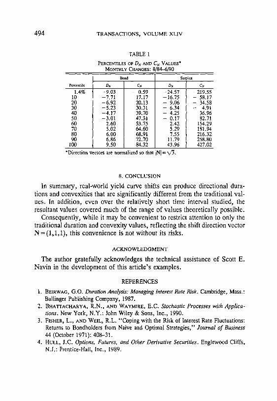
In addition to these range observations, note that the extreme observations were not true "outliers" of the full distribution of results. In particular, values throughout these ranges were observed, as the percentile data in Table 1 demonstrate. While the distribution of the DN(0) values gives insight to the proportion of "favorable" and "unfavorable" yield curve shifts, it is the distribution of ]D,v(0)], or absolute values, that gives information about the unit sensitivity created by the given shifts.

Of interest is that the bond duration of 6.16 is at the 57th percentile of the distribution of absolute values of the DN(0). That is, about 57 percent of the shifts created less unit sensitivity than the duration implied, while 43 percent created more. For surplus, the duration of 4.85 is at the 31st percentile of absolute values, implying that this value understated unit sensitivity for 69 percent of the shifts during this period.

For the distribution of CN(0) values, both the bond convexity of 52.41 and the surplus convexity of 140.52 are seen to be at about the 55th percentile value of the respective distributions.


TABLE 1

PERCENTILES OF D N AND C~ VALUES* MONTHLY CHANGES: 8/84--6190

Bond Surplus

Percentile DN

1 . 4 %

I0 20 30 40 5O 6O 70 80 90

100

D N C #

--9.03 -- 0.59 --7.71 17.17 -6.92 20.13 -5.23 30.31 -4.17 39.70 -3.01 47.31

2.60 53.75 5.02 64.60 6.00 68.91 6.86 72.70 9.50 84.32

*Direction vectors are normalized so that

- 24.57 - 16.75 - 9.06 - 6.34 - 4.25 - 0.17

2.42 5.29 7.55

11.79 43.96

CN

-219.55 - 58.17 - 34.58 - 4.91

36.96 82.71

154.29 181.94 216.32 268.80 427.02

8. CONCLUSION

In summary, real-world yield curve shifts can produce directional durations and convexities that are significantly different from the traditional values. In addition, even over the relatively short time interval studied, the resultant values covered much of the range of values theoretically possible.

Consequently, while it may be convenient to restrict attention to only the traditional duration and convexity values, reflecting the shift direction vector N = (1,1,1), this convenience is not without its risks.

ACKNOWLEDGMENT

The author gratefully acknowledges the technical assistance of Scott E. Navin in the development of this article's examples.

REFERENCES

1. BEIRWAG, G.O. Duration Analysis: Managing Interest Rate Risk. Cambridge, Mass.: Ballinger Publishing Company, 1987.

2. BHATTACHARYA, R.N., AND WAYMmE, E.C. Stochastic Processes with Applica- tions. New York, N.Y.: John Wiley & Sons, Inc., 1990.

3. FtSHER, L., AND WEIL, R.L. "Coping with the Risk of Interest Rate Fluctuations: Returns to Bondholders from Naive and Optimal Strategies," Journal of Business 44 (October 1971): 408-31.

4. HULL, J.C. Options, Futures, and Other Derivative Securities. Englewood Cliffs, N.J.: Prentice-Hall, Inc., 1989.


5. KAHN, R.N., AND LOCHOFF, R. "Convexity and Exceptional Returns," Journal of Portfolio Management 16, no. 2 (Winter 1990): 43-47.

6. REITANO, R.R. "A Multivariate Approach to Duration Analysis," ARCH 1989.2: 97-181.

7. REITANO, R.R. "Non-Parallel Yield Curve Shifts and Durational Leverage," Jour- nal of Portfolio Management 16, no. 4 (Summer 1990): 62-67.

8. REITANO, R.R. "A Multivariate Approach to Immunization Theory," ARCH 1990.2: 261-312.

9. RmTANO, R.R. "Non-Parallel Yield Curve Shifts and Spread Leverage," Journal of Portfolio Management 17, no. 3 (Spring 1991): 82-87.

10. REITANO, R.R. "Multivariate Duration Analysis," TSA XLIII (1991): 335-92. 11. REITA~O, R.R. "Multivariate Immunization Theory," TSA XLIII (1991): 393-442. 12. REITANO, R.R. "Non-Parallel Yield Curve Shifts and Immunization," Journal of

Portfolio Management 18, no. 3 (Spring 1992): 36-43. 13. RmTANO, R.R. "Multivariate Stochastic Immunization Theory," TSA XLV (1993):

in press.

APPENDIX CONVEXITY AND STOCHASTIC CALCULUS

A.1 Introduction

While the calculus-based derivations of the properties of convexity are compelling, they are somewhat heuristic for at least the following reasons: (1) The value of positive convexity stems from Equation (4), but the in-

terval for Ai for which it holds is unspecified and could be too small to have practical value; equivalently, the omitted third-order term in the Taylor series could be very significant in practice.

(2) The conclusion that more positive convexity is better than less relies on the assumption that it is possible to fix duration, increase convexity, and not do so much harm to the omitted third-order term as to offset the intended benefit.

(3) If Ai is just "noise," that is, E[Ai] =0 and E[Ai 2] ¢0, why should convexity matter, ~,ince changes in rates will be offset "generally" by the opposite changes, simply returning the price to A(0)?

(4) All arguments ignore the time dynamic: What is the relationship between Ai and At? What is the dependence of price on time, independent of the change in rates, Ai?

The theory of stochastic calculus addresses these issues in a formal and concise way; see Hull [4] for an accessible account; Bhattacharya and Way- 1"hire [2] for more rigor. However, by assuming a simple asset such as a


zero-coupon bond, a good appreciation of this topic and its conclusions can be obtained by only algebraic manipulations and intermediate statistics. Fol- lowing this exercise, the more general model is addressed.

A.2 A Simple Example

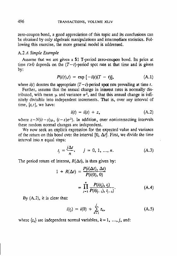
Assume that we are given a $1 T-period zero-coupon bond. Its price at time t>_0 depends on the (T-0-per iod spot rate at that time and is given by:

P(i(t),t) = exp [ - i ( t ) (T - t)], (A.1)

where i(t) denotes the appropriate (T-O-period spot rate prevailing at time t. Further, assume that the annual change in interest rates is normally dis-

tributed, with mean Ix and variance tr z, and that this annual change is infi- nitely divisible into independent increments. That is, over any interval of time, [s,t], we have:

i(t) = i(s) + z, (A.2)

where z - N ( ( t - s ) I x , ( t-s)tr2). In addition, over nonintersecting intervals these random normal changes are independent.

We now seek an explicit expression for the expected value and variance of the return on this bond over the interval [0, At]. First, we divide the time interval into n equal steps:

j A t tj = , j = 0, 1 . . . . . n. (A.3)

n

The period return of interest, R(At), is then given by:

1 + R(At) = P(i(At), At) e(i(o), o)

f l P(i(tj), ti) _ = j - 1 e ( i ( t j _ l ) ,

By (A.2), it is clear that: J

i(tj) = i(O) + 2 Zk, k=l

(A.4)

(A.5)

where {zk} are independent normal variables, k = 1, ..., j , and:


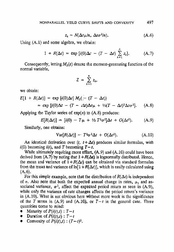
zk - N(At~/n, At0.2/n). (A.6)

Using (A.1) and some algebra, we obtaJ,n:

1 + R(At) = exp [i(0)A~;- (T - At) ~ zk]. (A.7) k=l

Consequently, letting Mz(s) denote the moment-generating function of the normal variable,

we obtain:

Z = ~ Zk, k=l

E[1 + R(At)] = exp [i(0)At] Mz(r' ( T - At))

= exp [ i ( o ) a t - ( T - ZXt),xt~ + V2(T- zXt)2±t0.2]. (A.8)

Applying the Taylor series of exp(:~) to (A.8) produces:

E[R(at)] = [i(0) - T~ + 1/2 T20.2]At + O(At2). (A.9)

Similarly, one obtains:

Var[R(At)] =: T2or2At + O(At2). (A.10)

An identical derivation over (t~, t+At ) produces similar formulas, with i(0) becoming i(t), and T becoming T - t ,

While ultimately requiring more effort, (A.9) and (A.10) could have been derived from (A.7) by noting that !1 +R(At) is lognormally distributed. Hence, the mean and variance of 1 +R(At) can be obtained via standard formulas from the mean and variance of ln[1 +R(At)], which is easily calculated using (A.6).

For this simple example, note that the distribution of R(At) is independent of n. Also note that both the expected annual change in rates, g,, and as- sociated variance, 0 -2, affect the expected period return as seen in (A.9), while only the variance of rate ehange,,s affects the period return's variance in (A.10). What is not obvious here without more work is the significance of the T terms in (A.9) and (A.10), or T - t in the general case. Three quantities come to mind: • Maturity of P(i(t),t) : T - t • Duration of P(i(t),t) : T - t • Convexity ofP(i( t ) , t ) : (T-- t )L


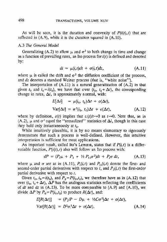
As will be seen, it is the duration and convexity of P(i(t),t) that are reflected in (A.9), while it is the duration squared in (A.10).

A.3 The General Model

Generalizing (A.2) to allow tx and 0.2 to both change in time and change as a function of prevailing rates, an lto process for i(t) is defined and denoted by:

di = Ix(i,t)dt + 0.(i,t)dz, (A.11)

where Ix is called the drift and 0 .2 the. diffusion coefficient of the process, and dz denotes a standard Weiner process (that is, "white noise").

The interpretation of (A.11) is a natural generalization of (A.2) in that given to and io=i(to) , we have that ever (to, to+At), the corresponding change in rates, Ai, is approximately normal, with:

E[Ai] = ~(io, to)At + o(At),

Var[Ai] = 0.2(6 , to)At + o(At), (A.12)

where by definition, o(t) implies that c(t)/t--*O as t ~ 0 . Note that, as in (A.2), ~z and 0.2 equal the "annualized" statistics of Ai, though in this case they hold only instantaneously at to.

While intuitively plausible, it is by no means elementary to rigorously demonstrate that such a process is well-defined. However, this intuitive interpretation is sufficient for most applications.

An important result, called Ito's Lemma, states that if P(i,t) is a differentiable function, P(i(t),t) also will follow an Ito process with:

dP = ( P ~ + P2 + V2 P~0.2)dt + P10.dz, (A.13)

where V. and o- are as in (A.11), P~(i,t) and PH(i,t) denote the first- and second-order partial derivatives with respect to i, and P2(i, t) the first-order partial derivative with respect to t.

Given t o, io =/(to), and Po =P(io,to), we therefore have as in (A.12) that over (to, to + At), AP has the analogous st atistics reflecting the coefficients of dt and dz in (A.13). To be more comparable to (A.9) and (A.10), we divide AP by Po =P(io,to) to produce R(At) , and:

E[R(At)] = (Pz/P - DIx + 1/zC0.2)At + o(At),

Var[R(At)] = DE0.?At + o(At) . (A.14)


In (A.14), D and C denote the duration and convexity of the price function evaluated at to and on io, while Pz/P equals the "earnings" rate of the price function at time to. Returning to (A.9) and (A.10), it is clear how the various components of those formulas reflect the features of the general formula in (A.14). Also, note that convexity influences the expected return of an asset from (A.14), and that this effect is first order in time.

Returning to the model in the paper, if the price function, P(i), is defined:

P(i) =- P(io + iN), (A.15)

so i = i(t) denotes the shift process in the direction of N from the initial yield curve io, the application of (A.14) is straightforward. That is, due to (18) and (26), the D and C of (A.14) become the directional counterparts, DN and CN.

Consequently, based on this more rigorous development, the heuristic approach of the paper is seen to capture the essence of the argument that positive convexity is good, and more is better, subject to the assumption that the yield curve shift complies with the direction vector assumed.

DISCUSSION OF PRECEDING PAPER

ELIAS S. W. SHIU."

Dr. Reitano is to be thanked for this paper, highlighting a deficiency in the classical immunization model. My discussion comprises two parts. The first part reinforces the theme of the paper that positive convexity may not necessarily be good and that more convexity may not necessarily be better. The second part elaborates on the continuous-time stochastic model intro- duced in the Appendix of the paper.

I. THE CLASSICAL MODEL

L 1. A Simple Example

Consider the simple situation in which the liability is a single cash flow to be paid at a future time T, and the assets backing the liability have a combined duration equal to T. Suppose that there is a change in the yield curve such that the interest rates before time T go down and the interest rates after time T go up. This means that the asset cash flows occurring before time T are to be reinvested at lower interest rates, and the asset cash flows occurring after time T have depreciated market values. Under such a shift in the term structure of interest rates, the surplus value of this block of business decreases, unless there are no asset cash flows occurring before or after time T. Indeed, under such a yield curve change, the larger the asset convexity, the larger the loss. This example of the negative effect of positive convexity can be generalized and developed more rigorously by using formula (D.20) in [9].

I. 2. The Barbell Strategy

An implication of Redington's theory is the barbell strategy. A financial intermediary issues or sells short a medium-term bond. The funds received are invested in long-term bonds and short-term bonds, with a combined duration matching that of the medium-term bond. As soon as there is an interest-rate movement, the long-term and short-term bonds are sold, and with the proceeds of the sale, the position in the medium-term bond is closed out. A positive profit is expected because, with the duration constraint, the convexity of the portfolio of long-term and short-term bonds is larger than that of the medium-term bond. Furthermore, the immunization model implies

501


that the larger the convexity of the asset portfolio, the larger the profit. To get a large convexity, the financial intermediary would invest in bonds of very short terms and also in bonds of very long terms. In other words, it would try to mismatch its assets and liabilities as much as possible while maintaining the duration constraint.

In Redington's model, this "barbell" strategy has an infinite rate of return because no fund at all is required from the financial intermediary for exe- cuting the strategy. The asset portfolio is funded entirely by the liability. In discussing Redington's paper, Rich [8] remarked: " I m m u n i z a t i o n . . . was an outstanding example of the difference between actuarial theory and practice. How delightful it would be if the funds of a life office could be so invested that, on any change in the rate of interest--whether up or down-- a profit would always emerge! But how difficult it would be to carry out to the full the investment policy implied by the theory of immunization." Forty years ago, Rich had anticipated the empirical findings of Kahn and Lochoff [6].

II. INTEREST RATES AS IT0 PROCESSES

II. 1. Continuous Price Processes Have Infinite Variation

In the Introduction of the Appendix, Dr. Reitano points out that, in the classical models, "[a]ll arguments ignore the time dynamic." This is one of his reasons for introducing a model in which interest rates are driven by an It6 process. I would like to present another motivation for such models by quoting the Harrison-Pitbladdo-Schaefer Theorem [3].

Consider a continuous-time financial model in which trading is continuous and frictionless. Suppose that the equilibrium price processes have continuous sample paths. It is shown in [3] that all but one of the price processes must have infinite or unbounded variation. The proof is by showing that, if there are two or more securities with bounded-variation price processes, there exist self-financing trading strategies with zero initial cost and positive profits subsequently; that is, there exist arbitrage opportunities. For price processes with continuous and bounded-variation sample paths, trading strategies can be defined in terms of Riemann-Stieltjes integrals. The proof of the theorem hinges on the chain rule and the change-of-variables formula for Riemann-Stieltjes integration.

DISCUSSION 503

A consequence of this theorem is that, in constructing a continuous-time financial model, to avoid internal inconsistencies (arbitrage opportunities), we may need to use stochastic processes such as It6 processes to model security prices and interest rates. Incorporating It6's stochastic calculus in the Fellowship examination syllabus was indeed a wise decision.

II. 2. Relationship between Convexity and Yield I am somewhat uneasy about the last sentence in the Appendix:

Consequently, based on this more rigorous development, the heuristic approach of the paper is seen to capture the essence of the argument that positive convexity is good, and more is better, subject to the assumption that the yield curve shift complies with the direction vector assumed.

However, I am not saying that it is incorrect. Let me explain my uneasiness with the following two points. Rewrite (A.13) as

dP ( - D ~ + y + ~ - ) d t - D c r d z (2.2.1) P

(As Dr. Reitano points out, "P2/P equals the 'earnings' rate of the price function." Thus

Pz/P = y(t),

the yield rate.) If we use the drift term in the right-hand side of (2.2.1) to justify that "positive convexity is good, and more is better," then we should also consider the contribution from -Dg. . With I~ positive, it seems that we should also conclude that "short duration is good, and shorter is better." My second point is that the clause "more is better" implies the existence of dominating strategies in the model, which, in turn, imply arbitrage opportunities in the model.

This problem disappears if we impose the principle of no arbitrage. Let

Q = Q(i , t )

denote the price function of another bond or bond portfolio, with duration D e, convexity Co, and yield rate Yo. Suppose that at time t, we have the duration-matching condition,

D(t) = DQ(t)


then a standard no-arbitrage argument ([10], pp. 180-181; [4], Section 12.1) shows that

from which, after cancelling the D~ terms, we obtain

y(t) + C(t)cr(i(t),t)2/2 = yQ(t) + CQ(t)cr(i(t),t)2/2. (2.2.2)

In the actuarial literature this yield-convexity relationship had been given by Levin ([7], p. 271). It implies that, among bonds of the same duration in a continuous-time equilibrium model, more convexity can be obtained only by accepting less yield.

11.3. Immunization

Given a continuous-time interest-rate model, the question of "continuous immunization" arises naturally. Consider a portfolio of assets and liabilities with matching value and duration initially. As time passes, the interest rates change and the asset duration and liability duration drift apart. By continuously trading the assets to maintain the duration-matching constraint, can the liability obligations always be met?

Let us consider a continuous-time financial model in which trading is continuous and frictionless; there exist one or more state variables whose current values completely specify all relevant information for investors; and these state variables are prescribed by It6 differential equations. In the sim- pler case of a single-state variable, that "continuous immunization" can be achieved by continuously rebalancing the portfolio to maintain the matching of the asset duration with the liability duration was proved by Boyle ([2], Section 3.7). Here, duration is defined with respect to the state variable. The asset and liability cash flows are assumed to be fixed and certain (the assets are not callable and the liabilities are not putable). There is no explicit condition on second- or higher-order terms such as convexity.

In the more general case of several state variables, that "continuous immunization" can be achieved by continuously rebalancing the portfolio to maintain the matching of each pair of asset and liability partial durations was proved by Albrecht ([1], Section 4). The partial durations are defined in terms of the state variables.

DISCUSSION 505

I1.4. Concluding Remarks

Frictionless market and continuous trading are idealized assumptions. In such models, arbitrages are excluded, and this has much intellectual appeal. On the other hand, these assumptions also imply that continuous security- price processes have infinite variation, which many may find unreasonable. By modeling the evolution of the term structure of interest rates using certain continuous stochastic processes of unbounded variation, we can derive the "continuous immunization" theorem, which is a reassuring result.

Let me conclude this discussion by quoting the eminent mathematician Mark Kac ([5], p. 699):

Models are, for the most part, caricatures of reality, but if they are good, then, like good caricatures, they portray, though perhaps in distorted manner, some of the features of the real world.

The main role of models is not so much to explain and to predict--though ultimately these are the main functions of science--as to polarize thinking and to pose sharp questions. Above all, they are fun to invent and to play with, and they have a peculiar life of their own. The "survival of the fittest" applies to models even more than it does to living creatures. They should not, however, be allowed to multiply indiscriminately without real necessity or real purpose.

Unless, of course, we all follow the dictum, attributed to Oswald Avery, that "you can blow all the bubbles you want to provided you are the one who pricks them."

REFERENCES

1. ALBRECHT, P. "A Note on Immunization under a General Stochastic Equilibrium Model of the Term Structure," Insurance: Mathematics and Economics 4 (1985): 239--44.

2. BOYLE, P.P. "Immunization under Stochastic Models of the Term Structure," Jour- nal of the Institute of Actuaries 105 (1978): 177--87.

3. HnRRISON, J.M., PITBLADDO, R., AND SCHAEFER, S.M. "Continuous Price Processes in Frictionless Markets Have Infinite Variation," Journal of Business 57 (1984): 353--65.

4. HULL, J. Options, Futures, and Other Derivative Securities, 2nd ed. Englewood Cliffs, N.J.: Prentice-Hall, 1993.

5. Knc, M. "Some Mathematical Models in Science," Science 166 (1969): 695-99. 6. KaHN, R.N., AND LOCHOFF, R. "Convexity and Exceptional Return," Journal of

Portfolio Management 16, no. 2 (Winter 1990): 43-47. 7. LEVIN, R. Discussion of Milgrom, P., "Measuring the Interest Rate Risk," TSA

XXXVII (1985): 267-75.


8. R~cH, C.D. Discussion of Redington, F.M., "Review of the Principles of Life- Office Valuations," Journal of the Institute of Actuaries 78 (1952)'. 319.

9. Smu, E. S.W. Discussion of Reitano, R.R., "Multivariate Immunization Theory," TSA XLIII (1991): 429-38.

10. VASICEK, O.A. "An Equilibrium Characterization of the Term Structure," Journal of Financial Economics 5 (1977): 177-88.

(AUTHOR'S REVIEW OF DISCUSSION)

ROBERT R. REITANO:

I thank Dr. Shiu for his insightful and complementary discussion; it adds significantly to the issues I address in my paper.

In Dr. Shiu's discussion of the "classical model," the simple example provides all the necessary insight--on why positive convexity need not be good, nor more better--that a more detailed and formula-driven demonstra- tion with partial convexities would provide. Clearly at the heart of this example is the potential effect of a nonparallel yield curve shift, specifically, a pivot-tilt shift through the maturity of the liability.

His discussion of the convexity implications for a barbell strategy, on the other hand, provides a very different insight, since only parallel shifts are assumed. Here it is demonstrated that if the yield curve moves in a parallel fashion only, infinite profits are possible with a simple management strategy: the positive barbell. The implication of this example and its risk-free arbitrage is that, not only is there the risk that the yield curve can move in a nonparallel fashion, but prospectively, there can be no valid argument to dismiss this possibility. Any such argument would have as its "logical" conclusion the opportunity for risk-free profits.

Turning next to his comments on It6 processes, I am especially grateful for his citing of the Harrison-Pitbladdo-Schaefer paper. While the It6 processes are known to have unbounded variation, I did not know whether this property was a necessary one for price processes, or if it is only the mathematical result of the intuitively appealing local behavior specified in my equation (A.12). Not surprisingly, as is the case so often in finance, the resolution depends on an arbitrage argument; that is, unbounded variation is necessary, except for at most one security.

Regarding his discussion of the relationship between convexity and yield, I have a couple of comments. First, in retrospect I think that the last sentence of my Appendix is a bit glib, especially for a "technical" paper, and is

DISCUSSION 507

incapable of withstanding the scrutiny Dr. Shiu affords it. Given that conces- sion, I agree with the second of his points, but not the first.

Dr. Shiu is quite right that convexity is not free, as the offending sentence implies, but rather, one must pay for it in terms of a lower earnings rate, denoted PJP in my Equation (A.14), or y in his Equation (2.2.1). He is also correct in pointing out that .Equation (2.2.2) is the "trade-off" formulation typically used. In practice, however, the buyer and seller rarely agree on the implications of Equation (2.2.2) for a given deal, since the implied trade-off materially reflects one's view of future yield volatility. Conse- quently, the buyer is likely to be more "bullish" on future volatility than the seller, or at least otherwise predisposed to being longer on convexity even given the "fair" price. It is in this context that my sentence was intended to be interpreted, in that if yield curve shifts are indeed parallel, more convexity is better than less for such a buyer.

On the other hand, I do not agree with his conclusion that an analogous statement can be made for duration, such as, "short duration is good, and shorter is better." The distinction I would make is based on the observation that duration returns are "signed," while convexity returns are "unsigned." That is, no matter how much positive or negative duration one has, losses are possible if yields shift the "wrong" way. For convexity, conversely, it is predictable that as long as yield curve shifts are parallel, positive convexity produces gains and negative convexity, losses, independent of the shift direction(s).

In closing, let me again thank Dr. Shiu for his informative and thought- provoking discussion and his additional references to the literature.

NONPARALLEL YIELD CURVE SHIFTS AND CONVEXITY ROBERT R. REITANO

Documents

Transcript of NONPARALLEL YIELD CURVE SHIFTS AND CONVEXITY ROBERT R. REITANO