
Nonlinear Wave Propagation in Photonic Crystal Fibers and Bose-Einstein Condensates
116
Nonlinear Wave Propagation in Photonic Crystal Fibers and Bose-Einstein Condensates Karen Marie Hilligsøe QUANTOP, Department of Physics and Astronomy & NKT Academy, Department of Chemistry University of Aarhus, Denmark PhD thesis February 2005
Transcript of Nonlinear Wave Propagation in Photonic Crystal Fibers and Bose-Einstein Condensates

Nonlinear Wave Propagation in
Photonic Crystal Fibers and
Bose-Einstein Condensates
Karen Marie HilligsøeQUANTOP, Department of Physics and Astronomy &
NKT Academy, Department of ChemistryUniversity of Aarhus, Denmark
PhD thesisFebruary 2005

ii
This thesis is submitted to the Faculty of Science at the University ofAarhus, Denmark, in order to fulfill the requirements for obtaining thePhD degree in Physics. The studies have been carried out at the Depart-ment of Physics and Astronomy under the supervision of Prof. SørenKeiding and Prof. Klaus Mølmer.

Contents
List of Publications vii
Abstract ix
1 Introduction to the thesis 11.1 Introduction . . . . . . . . . . . . . . . . . . . . . . . . . . . . . . . 21.2 Thesis outline . . . . . . . . . . . . . . . . . . . . . . . . . . . . . . 2
2 Photonic crystal fibers 52.1 Introduction . . . . . . . . . . . . . . . . . . . . . . . . . . . . . . . 62.2 Photonic crystal fibers . . . . . . . . . . . . . . . . . . . . . . . . . 6
2.2.1 Dispersion properties of PCFs . . . . . . . . . . . . . . . . . 72.2.2 Types of fibers . . . . . . . . . . . . . . . . . . . . . . . . . . 92.2.3 Applications . . . . . . . . . . . . . . . . . . . . . . . . . . . 9
2.3 Solving Maxwells equations . . . . . . . . . . . . . . . . . . . . . . 102.3.1 Dispersion properties . . . . . . . . . . . . . . . . . . . . . 112.3.2 Effective area . . . . . . . . . . . . . . . . . . . . . . . . . . 12
2.4 Conclusion . . . . . . . . . . . . . . . . . . . . . . . . . . . . . . . . 12
3 Model for wave propagation in photonic crystal fibers 153.1 Introduction . . . . . . . . . . . . . . . . . . . . . . . . . . . . . . . 163.2 The nonlinear Schrodinger equation . . . . . . . . . . . . . . . . . 163.3 Derivation of a nonlinear Schrodinger equation . . . . . . . . . . . 173.4 Dispersion . . . . . . . . . . . . . . . . . . . . . . . . . . . . . . . . 21
3.4.1 Calculation of the propagation constant . . . . . . . . . . . 213.4.2 Experimentally measured dispersion . . . . . . . . . . . . 21
3.5 Nonlinear effects . . . . . . . . . . . . . . . . . . . . . . . . . . . . 223.5.1 Raman response . . . . . . . . . . . . . . . . . . . . . . . . 223.5.2 Nonlinearity factor γ . . . . . . . . . . . . . . . . . . . . . . 223.5.3 Kerr nonlinearity . . . . . . . . . . . . . . . . . . . . . . . . 233.5.4 Overview of approached to the nonlinearity . . . . . . . . 23
3.6 Computational methods . . . . . . . . . . . . . . . . . . . . . . . . 243.6.1 Scaling . . . . . . . . . . . . . . . . . . . . . . . . . . . . . . 25
3.7 Conclusion . . . . . . . . . . . . . . . . . . . . . . . . . . . . . . . . 25
iii

iv CONTENTS
4 Supercontinuum generation 274.1 Introduction . . . . . . . . . . . . . . . . . . . . . . . . . . . . . . . 284.2 Applications . . . . . . . . . . . . . . . . . . . . . . . . . . . . . . . 294.3 Physical processes in supercontinuum generation . . . . . . . . . 30
4.3.1 Self phase and cross phase modulation . . . . . . . . . . . 314.3.2 Solitons . . . . . . . . . . . . . . . . . . . . . . . . . . . . . 314.3.3 Higher order dispersion . . . . . . . . . . . . . . . . . . . . 314.3.4 Non-solitonic radiation . . . . . . . . . . . . . . . . . . . . 324.3.5 Raman scattering and self-steepening . . . . . . . . . . . . 344.3.6 Four wave mixing . . . . . . . . . . . . . . . . . . . . . . . 354.3.7 Higher harmonics . . . . . . . . . . . . . . . . . . . . . . . 36
4.4 Supercontinuum evolution as a function of time and wavelength 374.4.1 Computational methods . . . . . . . . . . . . . . . . . . . . 37
4.5 Comparison with experiments . . . . . . . . . . . . . . . . . . . . 404.5.1 Comparison of spectra . . . . . . . . . . . . . . . . . . . . . 414.5.2 Phase-matched NSR . . . . . . . . . . . . . . . . . . . . . . 424.5.3 Threshold . . . . . . . . . . . . . . . . . . . . . . . . . . . . 424.5.4 Intensity of the nonsolitonic radiation . . . . . . . . . . . . 434.5.5 Wavelength of the nonsolitonic radiation . . . . . . . . . . 44
4.6 Conclusion . . . . . . . . . . . . . . . . . . . . . . . . . . . . . . . . 46
5 Four wave mixing in a photonic crystal fiber 475.1 Introduction . . . . . . . . . . . . . . . . . . . . . . . . . . . . . . . 485.2 PCF with two zero dispersion wavelengths . . . . . . . . . . . . . 485.3 Experiments . . . . . . . . . . . . . . . . . . . . . . . . . . . . . . . 505.4 Pulse evolution in the fiber . . . . . . . . . . . . . . . . . . . . . . . 51
5.4.1 Computational methods . . . . . . . . . . . . . . . . . . . . 565.5 Applications . . . . . . . . . . . . . . . . . . . . . . . . . . . . . . . 575.6 Phase-matched FWM - continuous wave regime . . . . . . . . . . 575.7 Conclusion . . . . . . . . . . . . . . . . . . . . . . . . . . . . . . . . 57
6 BEC in optical lattices 596.1 Introduction . . . . . . . . . . . . . . . . . . . . . . . . . . . . . . . 606.2 Fundamentals of BEC physics . . . . . . . . . . . . . . . . . . . . . 61
6.2.1 The two-body interaction potential . . . . . . . . . . . . . . 626.2.2 Second quantized Hamiltonian . . . . . . . . . . . . . . . . 636.2.3 The Bogoliubov approximation and mean field theory . . 636.2.4 The Gross-Pitaevskii equation . . . . . . . . . . . . . . . . 646.2.5 Elementary excitations . . . . . . . . . . . . . . . . . . . . . 656.2.6 One-dimensional nonlinear Schrodinger equation . . . . . 66
6.3 Bose-Einstein condensates in optical lattices . . . . . . . . . . . . . 676.3.1 The optical lattice . . . . . . . . . . . . . . . . . . . . . . . . 676.3.2 Linear description . . . . . . . . . . . . . . . . . . . . . . . 686.3.3 Nonlinear description . . . . . . . . . . . . . . . . . . . . . 696.3.4 General stability properties . . . . . . . . . . . . . . . . . . 70

CONTENTS v
6.3.5 Shallow lattices . . . . . . . . . . . . . . . . . . . . . . . . . 716.3.6 Deep lattices . . . . . . . . . . . . . . . . . . . . . . . . . . . 726.3.7 Superlattices . . . . . . . . . . . . . . . . . . . . . . . . . . . 73
6.4 Conclusion . . . . . . . . . . . . . . . . . . . . . . . . . . . . . . . . 73
7 Quantum beam splitting 757.1 Introduction . . . . . . . . . . . . . . . . . . . . . . . . . . . . . . . 767.2 Phase-matched four wave mixing . . . . . . . . . . . . . . . . . . . 777.3 Mean-field analysis . . . . . . . . . . . . . . . . . . . . . . . . . . . 777.4 Mean field results . . . . . . . . . . . . . . . . . . . . . . . . . . . . 79
7.4.1 Double four wave mixing . . . . . . . . . . . . . . . . . . . 807.5 Varying k0 . . . . . . . . . . . . . . . . . . . . . . . . . . . . . . . . 807.6 Rabi-oscillations . . . . . . . . . . . . . . . . . . . . . . . . . . . . . 827.7 Wave function in direct space . . . . . . . . . . . . . . . . . . . . . 847.8 Number state analysis . . . . . . . . . . . . . . . . . . . . . . . . . 85
7.8.1 Detuning . . . . . . . . . . . . . . . . . . . . . . . . . . . . . 877.8.2 Conclusion on number state analysis . . . . . . . . . . . . 88
7.9 Conclusion . . . . . . . . . . . . . . . . . . . . . . . . . . . . . . . . 88
8 Conclusion and perspectives 938.1 Conclusion and perspectives . . . . . . . . . . . . . . . . . . . . . 948.2 Acknowledgments . . . . . . . . . . . . . . . . . . . . . . . . . . . 97
Bibliography 99


List of Publications
[I] Stability of gap solitons in a Bose-Einstein condensate,K.M. Hilligsøe, M.K. Oberthaler and K.-P. Marzlin, Phys. Rev. A 66, 063605(2002).
[II] Coherent anti-Stokes Raman scattering microscopy with a photonic crystal fiberbased light source,H.N. Paulsen, K.M. Hilligsøe, J. Thøgersen, S.R. Keiding and J.J. Larsen,Opt. Lett., 28, 1123 (2003).
[III] Initial steps of supercontinuum generation in photonic crystal fibers,K.M. Hilligsøe, H.N. Paulsen, J. Thøgersen, S.R. Keiding and J.J. Larsen,J. Opt. Soc. Am. B., 20, 1887 (2003).
[IV] Supercontinuum generation in a photonic crystal fiber with two zero dispersionwavelengths,K.M. Hilligsøe, T.V. Andersen, H.N. Paulsen, C.K. Nielsen, K. Mølmer,S.R. Keiding, R. Kristiansen, K.P. Hansen and J.J. Larsen, Opt. Express, 12,1045 (2004),http://www.opticsexpress.org/abstract.cfm?URI=OPEX-12-6-1045.
[V] Continuous-wave wavelength conversion in a photonic crystal fiber with twozero-dispersion wavelengths,T.V. Andersen, K.M. Hilligsøe, C.K. Nielsen, J. Thøgersen, K.P. Hansen,S.R. Keiding and J.J. Larsen, Opt. Express, 12, 4113 (2004),http://www.opticsexpress.org/abstract.cfm?URI=OPEX-12-17-4113.
[VI] Phase-matched four wave mixing and quantum beam splitting of matter waves ina periodic potential,K.M. Hilligsøe and K. Mølmer,arXiv:cond-mat/0411228, accepted for publication in Phys. Rev. A, RapidCommunications.
vii


Abstract
Dansk resume.Denne afhandling beskæftiger sig med udbredelse af lys i fotoniske krystal-fibre. Lufthuller i længderetningen af denne nye type lyslederkabel er arsagtil fibrenes specielle egenskaber. Afhandlingen beskæftiger sig med, hvordanekstremt brede frekvensspektre dannes i fibrene. Andre har anvendt spek-trene til at udvikle en ny optisk frekvensstandard. Fire-bølge-blanding, hvorto lyskvanter forenes i fiberen og danner to nye, behandles. Processen kan po-tentielt anvendes til frekvenskonvertering i optiske netværk. Det andet emnei afhandlingen er Bose-Einstein kondensater i optiske gitre. Det undersøges,hvorledes to atomers impulser omdannes til to nye impulser gennem en fire-bølge-blandingsproces ækvivalent med fire-bølge-blandingen i fibrene.
Nonlinear wave propagation in photonic crystal fibers is a main theme in thisthesis. The fibers possess unique dispersive properties due to the transversemicro-structuring. The generation of supercontinua in the fibers caused by theinterplay between the dispersion and a cascade of nonlinear effects is investi-gated in the thesis. Already, the spectra have been used by others to developoptical frequency standards. For photonic crystal fibers with two closely lyingzero dispersion wavelengths phase-matched four wave mixing plays a dominat-ing role as shown in the thesis. The process can potentially be used for frequencyconversion in optical networks. The spectra generated in these fibers with fem-tosecond pulses can in principle be compressed to sub 15 femtoseconds. Theother system treated in the thesis is Bose-Einstein condensates in optical lattices.In this system the dispersive properties can be controlled by the optical latticemaking it possible to achieve phase-matched four wave mixing, resembling theprocess taking place in the photonic crystal fibers.
ix


C H A P T E R 1Introduction to the thesis
Wave propagation is a fundamental phenomenon occurring in several physicalsystems. This thesis will focus on two such systems: The propagation of light inphotonic crystal fibers and the propagation of matter waves in optical lattices.In this very brief chapter an outline of the thesis will be given.
1

2 Chapter 1. Introduction to the thesis
1.1 Introduction
Photonic crystals are periodic structures of dielectric materials and can todaybe produced with almost any imaginable structure. In this thesis focus will beon propagation of light in photonic crystal fibers (PCFs). These fibers are basedon a new and very promising technology and could provide solutions to manyoptical problems in telecommunications, light source manufacturing and hasalready revolutionized the field of frequency metrology.
The light itself can also provide periodic structuring through an optical lat-tice and in this system matter wave propagation will be investigated. It is onlya decade ago that Bose-Einstein condensation was first achieved in alkali gases[1, 2] and it has certainly turned into a very rich field since the condensatesare very flexible model systems for solid state physics and statistical physics ingeneral.
The dynamics of the wave propagation in both systems is mainly determinedby the interplay between dispersive and nonlinear effects. Consequently, eventhough the systems are fundamentally different, the physical phenomena arestill much the same. In Fig. 1.1 the two systems have been listed side by side.In the Bose-Einstein condensates (BECs) the nonlinear response originates inthe s-wave scattering between atom pairs, whereas the nonlinearity in the PCFsstems from saturation and optical pumping accounted for through a nonlinearsusceptibility. The micro-structuring of the PCFs leads to unique and tailorabledispersive properties. In the Bose-Einstein condensed system the optical latticedoes the job of tuning the dispersion.
In many situations the systems can be described by a type of nonlinear Schrodingerequation. In addition the behavior of the two systems is highly influenced byphase-matched processes such as four wave mixing, to which a great deal ofattention will be payed in this thesis.
1.2 Thesis outline
The outset for the work concerning the PCFs was the understanding of super-continuum generation in the fibers. Chapter 2 gives a short introduction to thebasic concepts of PCFs. In Chap. 3 a derivation of a general version of the non-linear Schrodinger equation is outlined. The chapters 4 and 5 are devoted to an-swering the following question: How does light propagate in a specific type ofPCF? In particular, Chap. 4 focuses on describing the evolution of light in a typ-ical PCF with only one zero dispersion wavelength, where emission of phase-matched non-solitonic radiation is a central process. This chapter is mainlybased on the paper [III]. Chapter 5 concerns the light propagation in a fiberwith two closely lying zero dispersion wavelength and is based on the paper[IV] with relations to paper [V]. In this fiber the determining process is insteadphase-mathced four wave mixing. Simulations are compared to experimentaldata obtained by the Femtosecond Group at the Department of Chemistry and

1.2 Thesis outline 3
the PCFs used in the experiments have been provided by the company CrystalFibre A/S.
The second part of the thesis concerns BECs in optical lattices and an in-troduction together with a brief review over the field is given in Chap. 6. Thefollowing central question in this part of the thesis was inspired by the role ofphase-matched four wave mixing in PCFs. Can phase-matched four wave mix-ing play a central role in a BEC in an optical lattice? The answer is yes andChap. 7 is devoted to the topic. This chapter is based on paper [VI], whereasthe paper [I] is not explicitly treated in this thesis, since it relates to my Master’sthesis work. Finally Chap. 8 closes the thesis with a conclusion and perspectivesfor further research.

4 Chapter 1. Introduction to the thesis
NonlinearSchrödinger
Equation
NONLINEARITY
+
DISPERSION
Phase-matchedprocesses:
Four Wave Mixing
Non Solitonic Radiation
NONLINEAR ATOM OPTICSRef. [I], [VI]
s-wave scattering
Kinetic energy
Periodic potential
Ref. [VI]
NONLINEAR FIBER OPTICS
Ref. [II]-[V]
Nonlinear susceptibiliy
Material dispersion
Micro structuring
Ref. [IV], [V]
Ref. [III]
Figure 1.1: The dynamics of light propagation in PCFs and evolution of matterwaves in optical lattices are basically determined by the interplay between disper-sive and nonlinear effects. A nonlinear Schrodinger equation is often sufficient todescribe the wave propagation in both systems. Phase-matched processes play im-portant roles in the systems and the papers [IV-V] are treating four wave mixingin PCFs, whereas the paper [VI] concerns four wave mixing in a BEC in an opticallattice. The paper [III] is examining the production of phase-matched non-solitonicradiation in PCFs.

C H A P T E R 2Photonic crystal fibers
An introduction to PCFs is given. More thorough introductions to the field aregiven in the review articles [3, 4] and the book [5]. In this chapter it is fur-thermore sketched how the frequency dependent propagation constant and theeffective area of the fibers can be found.
5
6 Chapter 2. Photonic crystal fibers
2.1 Introduction
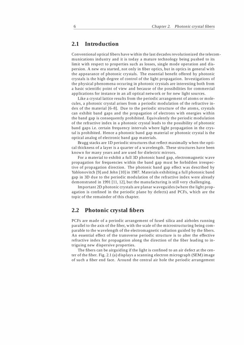
Conventional optical fibers have within the last decades revolutionized the telecom-munications industry and it is today a mature technology being pushed to itslimit with respect to properties such as losses, single mode operation and dis-persion. A new era started, not only in fiber optics, but in optics in general withthe appearance of photonic crystals. The essential benefit offered by photoniccrystals is the high degree of control of the light propagation. Investigations ofthe physical phenomena occuring in photonic crystals are interesting both froma basic scientific point of view and because of the possibilities for commercialapplications for instance in an all optical network or for new light sources.
Like a crystal lattice results from the periodic arrangement of atoms or mole-cules, a photonic crystal arises from a periodic modulation of the refractive in-dex of the material [6–8]. Due to the periodic structure of the atoms, crystalscan exhibit band gaps and the propagation of electrons with energies withinthe band gap is consequently prohibited. Equivalently the periodic modulationof the refractive index in a photonic crystal leads to the possibility of photonicband gaps i.e. certain frequency intervals where light propagation in the crys-tal is prohibited. Hence a photonic band gap material or photonic crystal is theoptical analog of electronic band gap materials.
Bragg stacks are 1D periodic structures that reflect maximally when the opti-cal thickness of a layer is a quarter of a wavelength. These structures have beenknown for many years and are used for dielectric mirrors.
For a material to exhibit a full 3D photonic band gap, electromagnetic wavepropagation for frequencies within the band gap must be forbidden irrespec-tive of propagation direction. The photonic band gap effect was described byYablonovitch [9] and John [10] in 1987. Materials exhibiting a full photonic bandgap in 3D due to the periodic modulation of the refractive index were alreadydemonstrated in 1991 [11, 12], but the manufacturing is still very challenging.
Important 2D photonic crystals are planar waveguides (where the light prop-agation is confined in the periodic plane by defects) and PCFs, which are thetopic of the remainder of this chapter.
2.2 Photonic crystal fibers
PCFs are made of a periodic arrangement of fused silica and airholes runningparallel to the axis of the fiber, with the scale of the microstructuring being com-parable to the wavelength of the electromagnetic radiation guided by the fibers.An essential effect of the transverse periodic structure is to alter the effectiverefractive index for propagation along the direction of the fiber leading to in-triguing new dispersive properties.
The fibers can be airguiding if the light is confined to an air defect at the cen-ter of the fiber. Fig. 2.1 (a) displays a scanning electron micrograph (SEM) imageof such a fiber end face. Around the central air hole the periodic arrangement

2.2 Photonic crystal fibers 7
of air and silica is seen to form a 2D photonic crystal structure. (One can saythat the 2D photonic crystal forms the cladding of the fiber and the air hole inthe middle is the core of the fiber, where the light is guided). In this fiber light isguided by the photonic band gap (PBG) effect. Frequencies within a band gapof the structure will experience multiple Bragg reflection leading to destructiveinterference of light trying to propagate away from the air core. The function ofthe air core is to provide a defect in the periodic structure in which the propaga-tion of frequencies inside the band gap is actually allowed. Consequently, onespeaks of a mode inside the band gap and this type of fiber is called a photonicband gap fiber. They were first demonstrated by P. St. J. Russell’s group in Bath[13, 14].
Another possibility is to let the central defect be made of silica instead ofair as seen on Fig. 2.1 (b). This type of fiber was also first demonstrated by thegroup in Bath [15]. The 2D photonic crystal around the core has an effectiverefractive index between that of silica and air. Therefore, the light guidancecan be explained by total internal reflection (TIR), which is also the way light isguided in step index fibers. These fibers with a central material defect are hencereferred to as index guiding fibers. Wave propagation in these fibers is a majortopic in this thesis.
(a) (b)
10 µm
Figure 2.1: (a) SEM-image of a fiber in which light is guided by the photonic bandgap effect. The light is guided in the big airhole (center of picture), which is sur-rounded by hollow silica tubes. The diameter of the central airhole is 9.3 µm. (b)SEM-image of a PCF where the light is guided in the central core defect by totalinternal reflection. The dark parts of the picture indicate the airfilled regions, thebrighter parts the fused silica. Pictures provided by Crystal Fibre A/S.
2.2.1 Dispersion properties of PCFs
In a homogeneous medium the dispersion relation between wave vector k andfrequency ω of the propagating light is given through the refractive index of thematerial ω = c|k|/n. In a PCF it is the combined effect of the material dispersion

8 Chapter 2. Photonic crystal fibers
and the band structure arising from the 2D photonic crystal that determines thedispersion characteristics of the fiber. For propagation in fibers it is the disper-sion for the wave vector component along the z-direction kz that is the interest-ing parameter. In the fiber optics literature kz is referred to as the propagationconstant β. It is then reasonable to define an effective refractive index as
neff =βc
ωfund., (2.1)
where ωfund. denotes the frequencies of the lowest lying mode in the fiber.The higher derivatives of the propagation constant are given as
βn(ω) =∂nβ
∂ωn, (2.2)
and the second order dispersion D = −2πcλ2 β2 is just another way of expressing
β2. The zero-dispersion wavelength (λZD) is defined as the free space wave-length λ = 2πc/ω where β2 = 0.
A cross-section of an index guiding PCF is shown in Fig. 2.2 and in Sec. 2.3a calculation of the dispersion properties and effective area of this fiber will besketched. The dispersion given by β2(λ) is shown in Fig. 2.3 (a) and the fiber hasλZD = 721 nm, whereas the zero dispersion wavelength for bulk silica is foundaround 1300 nm. The zero dispersion wavelength for this fiber has consequentlybeen shifted into the visible regime due to the micro-structuring. This widelytunable group velocity dispersion is an extremely valuable property of the PCFs.The dispersion can be tuned by a proper choice of the size of the airholes, thedistance between the holes (pitch) and the size of the central defect. A generaltendency is that the zero dispersion wavelength is found at a shorter wavelengthwhen the fraction of airfilling is increased and the central defect is decreased [5].It is possible to manufacture fibers with zero dispersion wavelengths between500 and 1500 nm. Another general trend is that decreasing either the pitch orthe hole-size leads to a higher curvature of the dispersion profile, eventuallyleading to two closely lying zero dispersion wavelengths. The effects of thisfiber dispersion will be treated in detail in Chap. 5.
The fibers can be made with cores down to 1 µm in diameter. Due to thesmall core areas huge intensities can be obtained in the cores of the fibers. Con-sequently, such fibers will exhibit a highly nonlinear response.
Another very useful property of the fibers is that they can be made endlesslysingle mode. Only one mode should have a propagation constant between theeffective propagation constants for the cladding and the core i.e. ncorek > β >ncladk, where k is the free space propagation constant. The restriction corre-sponds to only one solution to Maxwell’s equations propagating in the core andevanescent in the cladding. The effective frequency parameter is given by [13]
Veff = (2πρ/λ)√n2
core − n2clad, (2.3)
where ρ is the core radius. For the fiber to be single mode Veff should be below2.405. As λ decreases, the effective index of the cladding nclad increases, because

2.2 Photonic crystal fibers 9
more intensity of the light will be confined to the silica part of the cladding.Consequently, Veff can be kept below 2.405 for a wide range of wavelengths andthe fiber is said to be endlessly singlemode. In this way fibers, even with a verylarge core, can be made endlessly singlemode [16].
As the mode area of the fiber increases the relative intensity in the core willdecrease. Hence the fibers can be used for linear propagation, where a lot ofpower can be delivered without going into a nonlinear propagation regime.
2.2.2 Types of fibers
Microstructured fibers have also been produced from polymers [17] and softglass [18]. The low index material need not be air, although air of course hasthe advantage of providing a very low refractive index and consequently thepossibility for a high index contrast.
The PCFs have been doped with optically active rare earth elements such asEr, Yb, Th and Nd, making the fibers very attractive candidates for laser action.Furthermore, fibers with double claddings have been manufactured and lasershave been demonstrated with pumping into the inner cladding and lasing in thecore [19–23].
There are innumerable possibilities for geometries of the fibers. Furthermorethe systems are scalable, since the propagation in the structures are determinedby Maxwell’s equations. Of course the material dispersion of silica due to theresonances in the material is given beforehand.
The fibers can furthermore be produced with double cores, with possibilitiesfor interactions and coherence of the light between the cores. By breaking thesymmetry of the fiber, for instance by an elliptical core the fibers can be madepolarization maintaining [24].
2.2.3 Applications
In telecommunication the fibers could provide many new solutions. The PBGfibers offer the possibility of low losses and dispersion, a possible competitor toconventional fibers [25].
The development of all optical networks could benefit from the index guid-ing PCFs, for instance with respect to optical switching [26] and wavelengthconversion based on four wave mixing [27, 28], which it treated in Chap. 5.
The PBG fibers can act as flexible systems for atom optics. They can be filledwith gases, and for instance Raman scattering of hydrogen has been investi-gated [29]. They can also act as wave-guides for matter waves if a dipole field issuperimposed. The interactions with gases or liquids in the air holes of both theindex guiding fibers and the fibers guiding by the PBG effect show interestingpotentials for sensing purposes [30, 31]. Correlated pairs of photons, with po-tential applications in quantum optics, can be created in the fibers, for instancedue to the phase-matched degenerate four wave mixing that will be discussed in

10 Chapter 2. Photonic crystal fibers
Chap. 5. The fibers have also been used in quantum optics to produce squeezedlight through spectral filtering [32].
The generation of supercontinua was one of the first applications of the in-dex guiding PCFs. Optical spectra spanning more than an octave of frequenciescan be generated in the fibers and the spectra have already found a number ofapplications. The field of frequency metrology has been truly revolutionizedby the generation of supercontinua [33, 34] and frequency standards based onthe fibers are already commercially available. The continua have been used inoptical imaging techniques such as nonlinear coherent anti-Stokes scattering mi-croscopy [II] and optical coherence tomography [35]. Another application is aswavelength division multiplexing light sources, but the noise in the spectra isa challenge in this respect [36]. Since the initial demonstration of the supercon-tinua by Ranka et al. [37] a huge research effort has been put into identifyingthe processes and controlling the properties responsible for the generation of thesupercontinua and it has definitely been a hot topic in optics.
Supercontinuum generation will be the topic of the following three chapters.Chapter 3 is devoted to a model for light propagation in the fibers in order tosubsequently investigate the supercontinuum generation. The dispersion char-acteristics and the effective transverse area of the fibers, serve as input para-meters in the model for wave propagation. In the following section it will besketched how these parameters can be calculated.
2.3 Solving Maxwells equations
To get the dispersion characteristics (ω versus β) of the fiber structure Maxwell’sequations have to be solved: Decoupling Maxwells equations with no free chargesand currents, assuming linear response of the medium and no losses leads to awave equation for the Hω(r) field
∇ ×[
1ε(r)
∇ × Hω(r)]
=(ω
c
)2
Hω(r) (2.4)
where ε is the dielectric function. Here the fields have been expanded into a setof harmonic modes Hω(r, t) = Re(Hω(r)e−iωt) with frequency ω. This can bedone without further loss of generality since Maxwell’s equations have alreadybeen assumed linear [6, 8]. Because of translational symmetry along the z-axisthe dielectric function only depends on (x, y), consequently the harmonic modescan be expressed on the following form:
Hω(r) =∑m
αmhm(x, y)e−iβ(m)(ω)z, (2.5)
where m denotes the mth eigenmode with transverse part hm(x, y) and prop-agation constant β(m)(ω). After expanding in a plane wave basis the matrixeigenvalue problem is solved leading to the (fully vectorial) eigenmodes. The

2.3 Solving Maxwells equations 11
method is described in [6, 38]. Johnson and Joannopoulos have developed afreely available code, to solve Maxwell’s equations [39]. With this code and adielectric function based on the SEM-image of Fig. 2.2 Niels Asger Mortensenand Jes Broeng from Crystal Fibre have calculated the transverse part hm(x, y)of the eigen modes and propagation constants β(m)(ω) [40].
Figure 2.2: SEM-image of the endface of a PCF with a core diameter of 1.7µm. Pic-ture provided by Crystal Fibre A/S.
2.3.1 Dispersion properties
Both the material dispersion of silica and the dispersion due to the micro-structuringof the fibers contribute to the effective refractive index of the fundamental mode
neff = nmaterial + neff,bandstructure − nconstant, (2.6)
The effective propagation constant β of the fundamental mode can subsequentlybe found from Eq. (2.1) by inserting neff.
The refractive index of silica nmaterial has been calculated from the Sellmeierformula
n2material(λ) = 1 +
p∑j=1
B2j
1 − (λj
λ
)2 , (2.7)
where λj is an atomic resonance in the fused silica. For the calculations theparameters given in [41] have been used: B1 = 0.6961663, B2 = 0.4079426, B3 =0.8974794, λ1 = 0.0684043µm, λ2 = 0.1162414µm, λ3 = 9.896161µm.
The contribution to the effective refractive index from the micro-structuringneff,bandstructure, has been calculated by assuming a frequency independent re-fractive index of silica (nconstant = 1.45) in the dielectric function ε(x, y) inEq. (2.4). By solving the equation the propagation constant of the fundamen-tal mode β(1) is found, giving neff,bandstructure = cβ(1)/ω.
To include the contribution to neff from silica only once, the constant offsetnconstant in Eq. (2.6) is introduced. In fact this constant term will have no impacton the simulations in the following chapters, since a frame of reference movingwith the group velocity of the propagating pulse is chosen.

12 Chapter 2. Photonic crystal fibers
500 1000 1500 2000−2000
−1000
0
1000
2000
λ [nm]
β 2[fs2 /c
m]
(a)
500 1000 1500 20001
1.5
2
2.5
3
λ [nm]
Aef
f [(µm
)2 ]
(b)
Figure 2.3: Dispersion characteristics for the fundamental frequency mode of the1.7µm core diameter PCF shown in Fig. 2.2. (b) Effective area of the same fiber.Calculations carried out by Niels Asger Mortensen / Jes Broeng from Crystal FibreA/S.
Based on a SEM-picture of the fiber end face shown in Fig. 2.2 the propaga-tion constant of the shown 1.7 µm core diameter PCF has been calculated usingthe method sketched above. The group velocity dispersion β2, calculated fromthe propagation constant, is shown on Fig. 2.3 (a). A mode corresponding to theother polarization state exists, but in the calculations presented in the followingchapters only propagation in one polarization mode will be considered, eventhough for example the fiber on Fig. 2.2 is not polarization maintaining.
The frequency dependency of the refractive index of silica can also be takeninto account initially through a frequency dependent dielectric function ε(x, y, ω).Equation (2.4) then has to be solved self consistently. When comparing the twomethods no major differences appear.
2.3.2 Effective area
An effective area of a mode in a fiber can be defined as [40, 41]
Aeff,n(ω) =
[ ∫dxdy|hn(x, y)|2]2∫dxdy|hn(x, y)|4 , (2.8)
where |hn(x, y)|2 is proportional to the intensity distribution in the fiber. Figure2.3 (b) shows the effective area of the fundamental mode for the 1.7 µm corediameter PCF. It is the high index contrast between silica and air that makes therelatively low effective areas in PCFs possible [40].
2.4 Conclusion
The transverse micro-structuring makes the dispersion of the fibers highly tun-able and together with the high index contrast it leads to the small effective area,

2.4 Conclusion 13
making high intensities in the fibers possible. Due to the high intensities a cas-cade of nonlinear effects can take place in the fibers. The interplay between thespecial dispersion of the fibers and these nonlinear effects makes the phenom-enon of supercontinuum generation possible. Chapter 4 and 5 will be devotedto investigations of supercontinuum generation.
Above, the linear Maxwell’s equations have been solved for the transversestructure of the fibers. Although the problem is nonlinear in its nature whenhigh intensities are involved, the method provides information about the prop-agation constant and the effective transverse area of the mode. These parame-ters will serve as input in the nonlinear model for wave propagation along thelength of the fiber. The model will be presented in the following chapter andwill subsequently be used to describe the generation of supercontinua in thefibers.


C H A P T E R 3Model for wave
propagation in photoniccrystal fibers
In this chapter it will be sketched how Maxwell’s equations together with a suit-able set of approximations lead to a nonlinear Schrodinger equation as a gov-erning equation for light propagation in PCFs. Subsequently several ways oftreating the dispersion and the nonlinearity will be treated. Finally the numeri-cal implementation will be addressed.
15

16 Chapter 3. Model for wave propagation in photonic crystal fibers
3.1 Introduction
The theoretical modelling of light propagation in the PCFs is needed, not onlyto get a good understanding of the processes taking place in supercontinuumgeneration, but also to give input to the design and development of new fiberstructures and applications.
A dedicated effort has been given to the understanding of supercontinuumgeneration in the PCFs, as can be seen from the substantial amount of publica-tions already on the subject. For modelling the propagation of light in the fibersa nonlinear Schrodinger equation has been applied [42–49].
A general version of the nonlinear Schrodinger equation that takes the Ra-man effects, the frequency dependence of the nonlinearity and the full disper-sion properties into account is presented in this chapter together with simplifiedversions of the equation. Numerical implementation and subsequent compari-son with experimental data illustrates the power of the model, suggesting thatthe behavior of “theoretical”, not yet produced fibers can be predicted. Themodel therefore provides a strong and flexible tool for the understanding andfurther development of the fibers. The derivation here much follows the lines ofderivations used for the propagation in conventional fibers [41, 50–52].
3.2 The nonlinear Schrodinger equation
The simplest form of the nonlinear Schrodinger equation is given by
d
dzA = −iβ2
2∂2
∂t2A+ iγ|A|2A, (3.1)
and it will be derived in the Sec. 3.3. On the way to the equation above a moregeneral version of the nonlinear Schrodinger equation will be found. The firstterm describes the second order dispersion determined by the material and thegeometrical structure of the fiber as described in the previous chapter. The sec-ond term is the nonlinearity, which depends upon the polarizability of the ma-terial through χ(3) and scales with the third power of the electric field. As men-tioned in Chap. 2 the PCFs can be designed to have a fundamental mode witha small transverse area resulting in high intensities inside the fiber, thereforenonlinear phenomena play important roles in the description of the fibers.
The nonlinear Schrodinger equation has been applied in fiber optics sincethe beginning of the eighties, where it was used to describe Mollenauer’s firstexperimental observations of solitons in optical fibers [53]. Solitons emerge asfundamental solutions to the nonlinear Schrodinger equation because the dis-persion term can balance the nonlinear term. With respect to supercontinuumgeneration in PCFs, soliton formation and decay play important roles, as will bedescribed in Sec. 4.3.
A nonlinear Schrodinger equation appears in other branches of physics aswell. In quantum optics the Gross-Pitaevskii equation is used to describe the

3.3 Derivation of a nonlinear Schrodinger equation 17
evolution of the Bose-Einstein condensate ground state wave function. Bose-Einstein condensates in optical lattices will be described in Chap. 6 and 7.
3.3 Derivation of a nonlinear Schrodinger equation
Decoupling Maxwell’s equations with no free currents and charges gives thefollowing wave equation for the electric field E(r, t)
∇ × ∇ × E(r, t) = − 1c2∂2
∂t2E(r, t) − µ0
∂2
∂t2P(r, t), (3.2)
where P(r, t) is the polarization, having a contribution from the linear polar-ization with susceptibility χ(1)(t − t1) and a contribution from the nonlinearpolarization with susceptibility χ(3), in the following approximated by
χ(3)(t− t1, t− t2, t− t3) = χ(3)g(t− t1)δ(t− t2)δ(t− t3). (3.3)
Through the delay-function g(t − t1) the interaction of the light with the vi-brational modes of silica can be included in the description (Raman scattering).χ(3)(t−t1, t−t2, t−t3) can be approximated by a product of three delta functionsif only the electronic response of the material is wanted, since it is almost instan-taneous, in which case one speaks of a Kerr nonlinearity. Because of inversionsymmetry of the fibers the second order polarization disappears.
Further the induced charges at the surfaces between air and silica are ne-glected, corresponding to assuming ∇ ·E(r, t) = 0 which leads to the followingapproximation
∇ × ∇ × E(r, t) = ∇(∇ · E(r, t)) −∇2E(r, t) −∇2E(r, t). (3.4)
Transforming to the frequency domain Using the following convention forFourier transforms
E(r, ω) =∫ ∞
−∞dt eiωtE(r, t) (3.5)
and the above listed approximations the wave equation 3.2 can be transformedto frequency space
∇2E(r, ω) + ε(x, y, ω)ω2
c2E(r, ω) = −µ0ω
2P3(r, ω) (3.6)
where
P3(r, t) = ε0χ(3)E(r, t)
∫ ∞
−∞dt1 g(t− t1)E2(r, t1) (3.7)
and ε(x, y, ω) = 1 + χ(1)(x, y, ω). As used in Chap. 2 the dielectric functiondoes not depend on the z coordinate because of translational symmetry alongthe z-axis.

18 Chapter 3. Model for wave propagation in photonic crystal fibers
Separating the electric field By assuming weak coupling between the trans-verse and longitudinal degrees of freedom through the nonlinearity, the electricfield can to a good approximation be separated into a product of a function withlongitudinal dependence G(z, ω) and a function with transversal dependenceh(x, y, ω) [50, 51]. Furthermore the fields are assumed to be linearly polarizedalong the vector x
E(r, ω) = xh(x, y, ω)√
S(ω)G(z, ω), (3.8)
where the normalization factor S(ω) is given by
S(ω) =∫dxdy |h(x, y, ω)|2. (3.9)
Equation 3.6 is separated into the following two equations
∇2⊥h(x, y, ω) + ε(r, ω)
ω2
c2h(x, y, ω) = β(ω)2h(x, y, ω), (3.10)
d2
dz2G(z, ω) + β(ω)2G(z, ω) = −ω
2
c2χ(3)
Aeff(ω)p(z, ω). (3.11)
The z-dependent nonlinear polarization is now given by
p(z, ω) =(
12π
)2 ∫dω1
∫dω2 g(ω1 − ω2)
×G(z, ω − ω1 + ω2)G∗(z, ω2)G(z, ω1), (3.12)
p(z, t) = G(z, t)∫dt1g(t− t1)G(z, t1)2. (3.13)
In the transverse equation (3.10) the nonlinearity has been completely ignored.In the longitudinal equation (3.11) the effective area Aeff(ω) below is introducedwhen integrating out the transverse degrees of freedom.
Aeff(ω) =
( ∫dxdy |h(x, y, ω)|2)2∫dxdy |h(x, y, ω)|4 . (3.14)
Equation Eq. (3.11) can in principle be implemented directly using for examplea Finite Difference Time Domain method (FDTD) [54, 55], but it is numericallyheavy.
Approximating second derivative The real electric field G(z, t) can always bewritten as
G(z, t) = Re[G+(z, t)] =12[G+(z, t) +G−(z, t)], (3.15)

3.3 Derivation of a nonlinear Schrodinger equation 19
where G−(z, t) = G+(z, t)∗. The Fourier transform of G(z, t) can be written asthe transform of the respective components as defined by Eq. (3.5)
G(z, ω) =12[G+(z, ω) + G−(z, ω)] =
12[U+(z, ω)eiβz + U−(z, ω)e−iβz]. (3.16)
Here the field has been written as a sum of a forward eiβz and backward e−iβz
propagating wave. For them to be distinguished and treated independently thewavepacket needs to consist of an interval of wavevectors, which is the case ifthe field can be described within a slowly varying envelope. If the forward andbackward propagating waves can be distinguished the following approximationfor the second derivative with respect to z can be made(
d2
dz2+ β(ω)2
)G+(z, ω) =
(d
dz+ iβ(ω)
)(d
dz− iβ(ω)
)G+(z, ω)
2iβ(ω)(d
dz− iβ(ω)
)G+(z, ω). (3.17)
Inserting G(z, t) in the polarization and collecting all terms effectively propa-gating forward leads to the following equation
d
dzG+(ω) = iβ(ω)G+(ω)
+ω2
c2χ(3)
8Aeff(ω)β(ω)
∫ ∞
−∞dt eiωt
∫ ∞
−∞dt1 g(t− t1)
×2G+(t)G+(t1)G−(t1) +G−(t)G+(t1)G+(t1)
+G+(t)G+(t1)G+(t1), (3.18)
where the z-dependence of G has been omitted. Had a plane wave G(z, t) =Re[ei(β0z−ω0t)] been considered and the time dependence on t1 ignored, all termsabove would be proportional to e−iω0t except the last term G+(t)G+(t1)G+(t1),which would be proportional to e−i3ω0t corresponding to third harmonic gener-ation.
For the approximation to be consistent the term corresponding to third har-monic generation has to be neglected, since the coupling from the forward prop-agating component (ω0) to the third harmonic (3ω0) is in principle the same asbetween the forward (ω0) and backward (−ω0) propagating components.
Shift of central wavelength It is numerically practical to center the spectrumaround ω0 defining a new frequency variable ω1 = ω − ω0. The new field isdefined as G′
+(t) = G+(t)eiω0t. Shifting the center frequency does not implya further approximation. The essential approximation was made above wherethe forward and backward propagating waves were assumed distinguishable.It has been argued [50] that the approximation is valid for spectra as broad asω0/3. The simulations carried out in the following chapters go beyond this limitand still provide reasonable results.

20 Chapter 3. Model for wave propagation in photonic crystal fibers
In the following equation a coordinate transformation to a frame of referencemoving with velocity 1/β1 is made with z′ = z, t′ = t − β1z, d/dz = d/dz′ −β1d/dt
′
d
dz′G′
+(ω1) = i(β(ω) − β1ω)G′+(ω1)
+ω
c
χ(3)
8Aeff(ω)n0
∫ ∞
−∞dt′ eiω1t′
∫ ∞
−∞dt′1 g(t
′ − t′1)
×2G′+(t′)|G′
+(t′1)|2 +G′∗+(t′)G′2
+(t′1)ei2ω0(t
′−t′1). (3.19)
The propagation constant in the nonlinear term has here been approximated byβ(ω) = n0ω/c, where n0 = neff(ω0).
Units of electric field The input electric field can be written as
G′(z′, t′) = Gu(z′, t′), (3.20)
where u(z, t) is expressed in dimensionless units. An effective power P of thelight in the fiber is then given by
P =12ε0n0c|G|2, (3.21)
Consequently, by introducing the field
A(z′, t′) =√Pu(z′, t′) =
√ε0n0c
2Gu(z′, t′) =
√ε0n0c
2G′(z′, t′), (3.22)
the electric field is expressed in units of power. The propagation equation forthe field A is then given by
d
dzA(ω1) = i(β(ω) − β1ω)A(ω1) (3.23)
+iγ(ω)∫ ∞
−∞dt eiω1tA(t)
×∫ ∞
−∞dt1 g(t− t1)|A(t1)|2,
where the primes on the t, z coordinates have simply been removed, but themoving frame of reference is retained. A term A(t)∗A(t1)2ei2ω0(t−t1) has beenapproximated with A(t)|A(t1)|2. The convention in [41, 56] for the real part ofthe nonlinear refractive index n2 = 3χ(3)
4ε0cn20
has been used. For the nonlinearityfactor the convention suggested in [41] has been followed
γ(ω) =n2ω
cAeff(ω). (3.24)
Eq. (3.23) can be directly implemented. The following sections will go throughvarious ways of treating the dispersion and the nonlinearity in the equation.

3.4 Dispersion 21
3.4 Dispersion
The propagation constant can be achieved either from calculations or experi-mental investigations of the fiber and is often expressed in terms of a Taylorexpansion
β(ω) = neff(ω)ω/c =∑m
1m!βm(ω − ω0)m; βm =
∂mβ
∂ωm
∣∣∣∣∣ω=ω0
. (3.25)
Any dispersion profile can be fitted with a Taylor polynomial, the question isonly how many terms are needed to make a good fit over the width of the spec-trum.
3.4.1 Calculation of the propagation constant
The propagation constant β(ω) appearing in Eq. (3.11) can be found via the cal-culations presented in Chap. 2. The linear part of Eq. (3.11)
d2
dz2G(z, ω) = −β(ω)2G(z, ω), (3.26)
and Eq. (2.4) both originate from Maxwell’s linear equations. By considering themagnetic field Hω(r) as given by Eq. (2.5) and taking the second derivative withrespect to z the following equation arises
d2
dz2Hω(r) = −β(ω)2Hω(r). (3.27)
The magnetic and electric fields are related by
Eω(r) = − ic
ωε(x, y)∇ × Hω(r), (3.28)
where with translational symmetry ε(x, y) is independent of z. Consequently,Eω(r) also fulfills Eq. (3.26) and β(ω) in this and the previous chapter is thesame.
3.4.2 Experimentally measured dispersion
A white-light interferometer [57] can be used to measure the second order dis-persion of the PCFs. The Femtosecond Chemistry group has build such an inter-ferometer and measured the fiber dispersion β2(ω), which can be integrated togive the propagation constant. The integration constants will not have influenceon the propagation simulations, since the evolution of the pulses is followed ina frame moving with the group velocity of the pulse. Calculated and measureddispersion can be compared and the importance of the deviation can be revealedby the simulations described in this chapter.

22 Chapter 3. Model for wave propagation in photonic crystal fibers
3.5 Nonlinear effects
As mentioned, Eq. (3.23) can be implemented directly as it is including both fullfrequency dependency of the propagation constant and the effective area as wellas self-steepening and Raman effects.
3.5.1 Raman response
For the Raman response function the expression g(t) = (1 − fR)δ(t) + fRgR(t)has been used, where the delta function term originates from the electronic re-sponse i.e. the Kerr interaction and the last term takes the Raman scattering intoaccount. The function gR(t) can be chosen on the form
gR(t) =τ21 + τ2
2
τ1τ22
e−t/τ2sin(t/τ1); t > 0, (3.29)
gR(t) = 0; t < 0, (3.30)
as given by [50]. Raman scattering can be explained as scattering of light onthe optical phonons and 1/τ1 gives the optical phonon frequency. 1/τ2 gives thebandwidth of the Lorentzian line. The same values as in [41] have been appliedfor the constants: τ1 = 12.2fs, τ2 = 32fs, fR = 0.18.
3.5.2 Nonlinearity factor γ
The frequency dependent nonlinearity factor γ(ω) in Eq. (3.24) is found fromthe effective area Aeff(ω) as calculated in Chap. 2.
Since the effective area Aeff(ω) often does not vary too drastically with fre-quency as seen on Fig. 2.3 (b) a valuable approximation is to assume the effectivearea to be constant Aeff,0. With this approximation the nonlinearity factor can bewritten as
γ(ω) =n2ω
cAeff,0= γ0
(1 +
ω1
ω0
), (3.31)
where ω0 = ω − ω1 is the frequency of the input pulse and γ0 = n2ω0cAeff,0
. With thisnonlinearity factor the nonlinear Schrodinger equation is given by
d
dzA(ω1) = i(β(ω) − β1ω)A(ω1) + iγ0
(1 +
ω1
ω0
)
×∫ ∞
−∞dt eiω1tA(t)
∫ ∞
−∞dt1 g(t− t1)|A(t1)|2, (3.32)
and this equation will be used extensively for the simulations in the followingtwo chapters.

3.5 Nonlinear effects 23
In the time domain the nonlinearity factor above is given by γ0
(1 + i 1
ω0
∂∂t
),
where the time derivative takes self-steepening and shock formation into ac-count. Consequently, for very long pulses this time derivative can be omittedcorresponding to assuming a constant nonlinearity factor
γ(ω) = γ0. (3.33)
If the computational grid is centered at a frequency ωc different from the centralfrequency of the pulse ω0 the nonlinearity factor has to be changed accordinglyγ0 = n2ωc
cAeff,0.
3.5.3 Kerr nonlinearity
A Kerr nonlinearity can be assumed by ignoring the Raman response in thefibers corresponding to setting g(t) = δ(t). If the nonlinearity factor is assumedconstant γ = γ0 the following equation arises
d
dzA(ω1) = i(β(ω) − β1ω)A(ω1) + iγ0
∫ ∞
−∞dt eiω1tA(t)|A(t)|2. (3.34)
If all terms are transformed to the time domain and only up to second orderdispersion is taken into account the following equation appears
d
dzA(t) = −iβ2
2∂2
∂t2A(t) + iγ|A|2A(t). (3.35)
This is exactly the simple form of the nonlinear Schrodinger equation (3.1) statedin the beginning of this chapter.
3.5.4 Overview of approached to the nonlinearity
Most of the approximations mentioned in this section can be applied indepen-dently
• Response function g(t):
→ Raman scattering g(t) = (1 − fR)δ(t) + fRgR(t).
→ Kerr nonlinearity g(t) = δ(t).
• Nonlinearity factor γ(ω) = n2ωcAeff(ω) :
→ Effective area: Frequency dependent Aeff(ω) or constant Aeff,0.
→ Self-steepening and shock formation: Included ω = ω0(1 + ω1/ω0) ornot included ω = ω0.

24 Chapter 3. Model for wave propagation in photonic crystal fibers
Which method to choose is a question of computational time, available inputdata for β(ω) and Aeff(ω) and of the physical regime. Generally, for short pulses(<100 fs), high intensities (1011 W/cm2) and short propagation lengths (a fewcm) the error done by neglecting the Raman response of the material is limited(but is still there). For short pulses and high intensities the spectra generally getbroad because of self-phase modulation, consequently it is important to includethe frequency dependence of β(ω) and the effects of self-steepening and shockformation as in Eq. (3.32).
3.6 Computational methods
The equations have been implemented with the split step method with 4th or-der Runge Kutta steps for the nonlinearity. The dispersion is calculated in thefrequency domain. For the Fourier transformations the FFTW library has beenused [58]. The nonlinearity has been calculated implementing the two followingapproaches:
A: Direct integration of Raman response in the time domain.
In the first implementation of Eq. (3.32) the self-steepening term and the Ramanresponse integral were both evaluated in the time domain
d
dzA(ω1) = i(β(ω) − β1ω)A(ω1)
+∫ ∞
−∞dt eiω1t iγ0
(1 + i
1ω0
∂
∂t
)A(t)
×∫ ∞
−∞dt1 g(t− t1)|A(t1)|2, (3.36)
The time derivative was explicitly evaluated as
∂Y
∂t→ (Y [i+ 1] − Y [i− 1])/2∆t (3.37)
In the Raman response integral only the interval of response times from t−t1 = 0to 300 fs was included, since the influence of the Raman response beyond thistime is very limited.
B: Calculation of the Raman response convolution integral in the frequencydomain.
An alternative approach is to compute the Raman response integral by evaluat-ing the convolution in the frequency domain. Additionally, the time-derivativewas evaluated by multiplying with the frequency in the frequency domain. The

3.7 Conclusion 25
nonlinear term
X(ω1) = iγ0
(1 +
ω1
ω0
)F
(1 − fR)A(t)|A(t)|2
+fRA(t)∫ ∞
−∞dt1 gR(t− t1)|A(t1)|2
, (3.38)
could consequently be evaluated by making Fourier transformations F
Y (ω1) = FY (t) =∫ ∞
−∞dt eiω1tY (t), (3.39)
and inverse transformations F−1
Y (t) = F−1Y (ω1) =12π
∫ ∞
−∞dω1 e
−iω1tY (ω1). (3.40)
For each step dz the following transformations need to be carried out
Y (ω1) = F|A(t)|2, (3.41)gR(ω1) = FgR(t), (3.42)
I(t) =∫ ∞
−∞dt1 gR(t− t1)|A(t1)|2 = F−1Y (ω1)gR(ω1), (3.43)
M(ω1) = F(1 − fR)A(t)|A(t)|2 + fRA(t)I(t), (3.44)
X(ω1) = γ0
(1 +
ω1
ω0
)M(ω1). (3.45)
Method B is by far the fastest and most accurate since the time derivative andthe Raman response integral are treated as exact as possible with the given dis-cretization. In the following two chapters comparisons between the two imple-mentations will be given since unfortunately there is a small difference betweenthe two, mainly due to the evaluation of the time derivative in Eq. (3.37).
3.6.1 Scaling
The computation of the Fourier transformations scales as O(NlogN), where N isthe number of points in the grid. The z-step size depends on input intensity, thehigher the intensity, the faster is the dynamics consequently the more z-stepsare needed to propagate the same distance.
3.7 Conclusion
Starting with Maxwell’s equations it has been sketched how a nonlinear Schrodingerequation for wave propagation in the PCFs can be achieved. The full frequencydependency of the propagation constant as well as the effective transverse area

26 Chapter 3. Model for wave propagation in photonic crystal fibers
serve as input for the model and these parameters can either be calculated assketched in Chap. 2 or measured. The model includes the instantaneous non-linear response of silica. Additionally, the effects of Raman scattering, self-steepening and shock formation can be included. In the following chapter mostof the simulations shown will be based on Eq. (3.32) and the influence of thenonlinear effects will be investigated by comparison with the simpler versionEq. (3.34).

C H A P T E R 4Supercontinuum
generation
When a PCF is pumped with femtosecond pulses a supercontinuum is formedand the physical mechanisms at play in this process are investigated in thischapter. Simulations based on the model presented in the previous chapterserve to explain the scenario taking place when pulses propagate in the fibers.Subsequently the simulations are compared to experiments with good agree-ment. This chapter is mainly based on the article [III].
27

28 Chapter 4. Supercontinuum generation
4.1 Introduction
The generation of very broad spectra, called supercontinua, in PCFs has at-tracted much attention since Ranka et al. [37] demonstrated the first supercon-tinua in PCFs using low power titanium-sapphire laser pulses [59]. Supercon-tinua have previously been generated in gases, liquids, conventional and spe-ciality fibers. One advantage of using PCFs for supercontinuum generation isthe small effective area of the mode, leading to high intensities in the fibers.Consequently, nonlinear processes involved in the supercontinuum generationcan be significant even for relatively low pulse energies on the order of pJ forfemtosecond pulses. Input ranging from the continuous wave regime [60] allthe way to femtoseconds has been used. An additional advantage of the PCFs isthe unique dispersion of the fibers, effectively determining the dynamics of thesupercontinuum generation, one of the reasons being the possibility to controlthe phase-matching of several nonlinear processes.
In general, supercontinuum generation is based on a cascade of nonlinearprocesses well known from nonlinear optics like four-wave mixing, stimulatedRaman scattering and soliton dynamics. Today the generation can be controlledto a great extend by tailormade dispersion and appropriate choice of input pa-rameters [43–45, 47–49, 61, 62].
A specific example of supercontinuum generation is given on Fig. 4.1 wherea 1.7 µm core diameter PCF is pumped with 50 fs pulses at a wavelength of 800nm. After ∼ 20 cm of propagation the emerging light is projected on a screen asshown on the pictures. Going from (a) to (c) the input intensity increases andthe spectrum broadens. At the center of Fig. 4.1 (c) white light corresponding toa supercontinuum is generated. The remote field reveals the hexagonal micro-structuring of the fiber.
(a) (b) (c)
Figure 4.1: Supercontinuum generation in the 1.7 µm core diameter PCF pumpedwith 50 fs pulses at a wavelength of 800 nm. Input power is increasing from (a) to(c).
In this and the following chapter focus will be on the femtosecond regime,the regime in which supercontinua were first generated [37] and for which asubstantial amount of literature exists [44–49, 61, 63–67], [III, IV]. For a typicalPCF with a single zero dispersion wavelength, pumped in the anomalous dis-
4.2 Applications 29
persion regime, the dynamics of the supercontinuum generation is dominatedby the decay of higher order solitons emitting phase-matched radiation and thiswill be discussed in detail in the present chapter. For a fiber with a dispersionprofile with two closely lying zero dispersion wavelengths the dynamics is dom-inated by four wave mixing instead and the scenario in this type of fiber will bediscussed in Chap. 5.
Supercontinua have also been generated with pico-second and nano-secondpulses [44]. The nonlinear Schrodinger equation has been used to describe thegeneration of supercontia with pulses up to 60 ps long [42, 43]. 600 ps pulsesgenerated by Q-switching is treated in [68].
For the generation of supercontinua in the nano-second regime stimulatedRaman scattering as well as phase-matched four wave mixing play central roles.In fact a PCF pumped with 2-3 ns pulses has already been used by Koheras [69]in collaboration with the Helsinki University of Technology to make a commer-cially available white-light source.
Recently, supercontinua generated from continuous waves with powers of1.2-1.8 W were treated [60]. For these relatively high powers modulational in-stabilities cause the light to break up into solitons and in combination with in-trapulse stimulated Raman scattering the spectrum is broadened. The solitonscan subsequently emit phase-matched non-solitonic radiation, the same processas seen for the femtosecond pulses.
In general the importance of phase-matched processes such as four wavemixing increases with decreasing bandwidth of the pulses, corresponding to in-creasing length of the pulses. Another general tendency is, the higher the power,the broader the spectrum. The nonlinear response increases with increasing in-tensity and it is consequently easier to address the various nonlinear effects.
Recently the coherence properties and the influence of noise on the spectrahave been discussed. The input shot noise as well as the spontaneous Ramanscattering is amplified in the fibers. Short propagation lengths together withshort input pulses minimize the buildup of the noise [36, 63, 70].
4.2 Applications
Probably the most important application of supercontinua generated in PCFshas been in frequency metrology [33, 34, 71]. When a supercontinuum is gen-erated in a PCF with femtosecond pulses, the resulting spectrum consists of acomb of frequencies with equal spacing given by the laser repetition rate. Sincethe spectra can be made octave spanning, a frequency and the approximate dou-ble frequency exist in the spectrum and by beating the second harmonic of thelower frequency with the higher frequency a direct link between the repetitionrate and the optical frequency can be made. Consequently, a precise optical fre-quency standard can be established. Systems providing such optical frequencystandards are commercially available from a company related to the Munichgroup [72].

30 Chapter 4. Supercontinuum generation
As mentioned the supercontinua have also found an application within theinterferometric technique of optical coherence tomography, where they havelead to sub-micron resolution [35].
Another imaging technique where the supercontinua have been used as alight source is in coherent anti-Stokes Raman scattering (CARS) microscopy. Thetechnique has been used by the Femto Chemistry group [II] and the principle ofthis four wave mixing process is illustrated in Fig. 4.2 (a). The photon withfrequency ωS is provided by the laser and the ωP photons are generated in thePCF. When the energy difference ωP −ωS corresponds to a vibrational transition|1 > −|2 > in the sample, the signal with frequency ωAS will be resonantly en-hanced. The method has been used to achieve the picture of a yeast cell shown inFig. 4.2 (b), where the C-H stretch vibrational transition at 3000 cm−1 is probed.The cell contour as well as structure inside the cell (organelles) is seen.
ωP ωS
ωP ωAS
|1>|2>
(a) (b)
Figure 4.2: (a) Coherent anti Stokes Raman scattering. When the energy differenceωP − ωS corresponds to a vibrational transition in the sample |1 > −|2 > the signalwith frequency ωAS will be resonantly enhanced. (b) Picture of a yeast cell where theC-H stretch vibrational transition at 3000cm−1 is probed. The cell contour as wellas structure inside the cell (organelles) is clearly seen. The pictures are provided byHenrik Nørgaard Paulsen and Esben Ravn Andresen.
The supercontinua could serve as light sources for wavelength division mul-tiplexing where broad, stable, flat spectra are desirable, for many channels to becarved out. The noise in the spectra are still a challenge to overcome [36] for thesucces of this application.
The four wave mixing especially dominant in PCFs with two closely lyingzero dispersion wavelengths could be used as basis for a blue light source aswell as for wavelength converters. The dynamics in this type of fiber as well asthe perspectives for compression of the spectra will be treated in the followingchapter.
4.3 Physical processes in supercontinuum generation
This section gives a presentation of the various physical processes, which canplay a role when a supercontinuum is formed in a PCF. The effects important

4.3 Physical processes in supercontinuum generation 31
for the supercontinuum generation in the fiber shown in Fig. 2.2 will be empha-sized, since the simulations presented in this chapter are done for this fiber.
4.3.1 Self phase and cross phase modulation
The nonlinear response of the silica arises due to optical pumping of the energylevels for the electrons in silica as well as saturation effects for the transitions.The effects are described through the nonlinear polarization with susceptibilityχ(3). The self-phase modulation (SPM) can be explained through the nonlinearpart of the refractive index n2I . If the phase of the pulse is described by φ =βz − ω0t=(n + n2I(t))ω0z/c − ω0t new frequency components are generatedin the spectrum ω = −∂φ/∂t = −n2ω0z
c∂I(t)
∂t + ω0. The corresponding termin the nonlinear Schrodinger equation is γ|A|2A (the Kerr nonlinearity), whichis also responsible for the four wave mixing processes as well as cross phasemodulation, where it is simply the intensity of an other frequency component,which is responsible for the modulation of the phase. For femtosecond pulsesSPM plays an important role in the initial broadening of the spectra.
4.3.2 Solitons
The soliton is an exact solution to the nonlinear Schrodinger equation with Kerrnonlinearity and negative second order dispersion β2 as given in Eq. (3.1) and itphysically appears because the dispersion in the fiber is counteracted by SPM.The time evolution of an ideal third order soliton (N = 3) over 1 soliton period(z0) is shown on Fig. 4.3. The soliton number and period being defined as [41]
N2 =γP0T
20
|β2| , (4.1)
z0 =π
2T 2
0
|β2| . (4.2)
where γ = n2ω/(cAeff) is again the nonlinear coefficient, T0 = TFWHM/(2ln(1 +√2)) is the pulse duration and P0 is the peak power. After the soliton period
the pulse has reverted to its initial state as seen on Fig. 4.3, during the periodthe third order soliton contracts twice. If a fiber is pumped with a CW sourcein the anomalous dispersion regime, solitons can be generated as a consequenceof modulational instability. Performing a linear stability analysis on the CWlight in the fiber will reveal whether small modulations of the light will grow,corresponding to a modulational instability [41].
4.3.3 Higher order dispersion
Whereas higher order dispersion plays a minor role for pulse evolution in con-ventional fibers the special and often flat dispersion profiles often lead to highinfluence of the higher order dispersion terms.

32 Chapter 4. Supercontinuum generation
1
2
3
4
5
6
7
8
9
x 1010
z [m]
t [ps
]
0 0.1 0.2 0.3−1
−0.5
0
0.5
Figure 4.3: Propagation of a third order soliton.
The simulations in the left column of Fig. 4.4 are based on equation (3.34)using the full dispersion profile of the 1.7 µm core diameter fiber as shown onFig. 2.2. The input pulses had TFWHM=100 fs and were centered at λ=836nmwith an input intensity of I0 = 4.1 × 10¹⁰W/cm2 corresponding to a solitonnumber of 3.3. A constant effective area Aeff = 2(µm)2 and nonlinear refractiveindex n2 = 3 × 10⁻²⁰m2/W were used.
The frame of reference for the simulations can be chosen to move with anyvelocity. In Fig. 4.3 the velocity is equal to the group velocity of the soliton,which consequently stays centered at t=0 s. In Fig. 4.4 (a) the velocity is slightlydifferent from the group velocity of the pulse, which makes the center of thepulse shift to t<0 s. Apart from this shift of the center, due to the velocity off-set, the behavior of the pulses in Fig. 4.3 and Fig. 4.4 (a) is equivalent and welldescribed as the evolution of a higher (third) order soliton, also in the latter case.
Looking at the time evolution on the logarithmic scale Fig. 4.4 (b) revealsthat a new component has been formed as the soliton contracted after 4 cm.The component can be identified as the yellow line moving in the positive timedirection because it has a lower group velocity than the soliton. If a ”pure” thirdorder soliton is considered on a logarithmic scale no such component is formed,hence it must be attributed to the higher order dispersion.
Fig. 4.4 (c) depicts the pulse evolution in the frequency domain. As the soli-ton contracts in the time domain it broadens in the frequency domain. The hor-izontal line at λ=550 nm appears at the same point as the component in Fig. 4.4(b). The time wavelength plots in Fig. 4.8 described later will reveal that thetwo are indeed the same. From now on the component is named nonsolitonicradiation.
4.3.4 Non-solitonic radiation
One of several possible nonlinear phase-matched processes in the PCFs is thegeneration of non-solitonic radiation (NSR). The NSR is emitted as a disper-

4.3 Physical processes in supercontinuum generation 33
t [p
s]
(a)
0 0.05 0.1 0.15−1
−0.5
0
0.5
(d)
0 0.05 0.1 0.15−1
−0.5
0
0.5t
[ps]
(b)
0 0.05 0.1 0.15
−2
−1
0
1
2 (e)
0 0.05 0.1 0.15
−2
−1
0
1
2
Wav
elen
gth
[n
m] (c)
0 0.05 0.1 0.15
500
1000
1500
2000
(f)
0 0.05 0.1 0.15
500
1000
1500
2000
0.2
0.4
0.6
0.8
0
10
20
5
10
15
20
25
30
[a.u.]
z [m]
[a.u.]
x 1010 [a.u.]
Figure 4.4: Evolution of pulse along the fiber length. (a) Simulation with only Kerrnonlinearity based on Eq. (3.34) of the pulse intensity |A(z, t)|2. The behavior ofthe pulse resembles the behavior of the third order soliton in Fig. 4.3. (b) The samesimulation as shown in (a) but on a logarithmic scale log(|A(z, t)|2). A dispersivewave is emitted at z=4 cm, where the soliton contracts. (c) The spectral densitylog(|A(z, λ)|2) for the simulation shown in (a-b). A new frequency component ap-pears at λ=550 nm, this is the dispersive wave seen in (b). (d) Simulation of the pulseintensity |A(z, t)|2 including the effects of Raman scattering and self-steepeningbased on Eq. (3.32). Due to Raman scattering the soliton breaks up. (e) The samesimulation as shown in (d) but on a logarithmic scale, revealing the dispersive wavetogether with the broken-up soliton. (f) The spectral density log(|A(z, λ)|2) for thesimulation shown in (d-e).
sive wave around a wavelength phase-matched to the wavelength of the solitonwhen ∆φ = φS −φNSR = 0. φS is the phase of the soliton and φNSR is the phase

34 Chapter 4. Supercontinuum generation
of the nonsolitonic radiation and they are given by
φS =(β(ωS) +
n2IωS
c
)z − ωSt, (4.3)
φNSR = β(ωNSR)z − ωNSRt, (4.4)
where z is the propagated distance and β is again the propagation constant.For the phase-matching to occur the phases should be evaluated at the sametime t = z/vS , where vS is the group velocity of the soliton. The third term inEq. (4.3) accounts for self-phase modulation by the pump pulse with intensityI .
The phase difference ∆φ/z is plotted at Fig. 4.5 with λS=836nm. ∆φ = 0 atλ = 550nm, which is indeed the wavelength at which the nonsolitonic radiationwas observed. The explanation of the supercontinuum generation in terms of
400 600 800 1000 1200−6
−4
−2
0
2x 10⁴
λ [nm]
∆φ/z
[m−
1 ]
Figure 4.5: Phase difference ∆φ = φS − φNSR for λS = 836nm. Phase-matching∆φ = 0 is achieved for λNSR = 550 nm.
phase-matched NSR was originally given in [49].
4.3.5 Raman scattering and self-steepening
Figure 4.6 illustrates Raman scattering, which is a non-parametric process whereenergy is lost due to the vibrational excitation of the material. Raman scatter-ing is the origin of a self-frequency shift increasing with propagation length ofsolitons to longer wavelengths.
The self-steepening effect given through the time derivative of the nonlin-earity in the nonlinear Schrodinger equation is significant for short pulses.
Including Raman scattering and self-steepening in the nonlinear Schrodingerequation (3.32) gives the simulation results shown in the right column of Fig. 4.4.The important influence is that the soliton decays already the first time it con-tracts (i.e. after 4 cm). As seen on Fig. 4.4 (d-e) the soliton splits up, appearing

4.3 Physical processes in supercontinuum generation 35
|1>|0>|1>|0>
Figure 4.6: The excitation energy between the vibrational states |1 > and |2 > is lostto the material in the Raman scattering process.
as red traces in (e). The upper trace is a first order soliton self-frequency shiftingdue to intrapulse Raman scattering, consequently the trace bends. The lowertrace is the remaining pulse that starts to diverge into two solitons, the initialthird order solitons therefore splits into three first order solitons, with differentintensities.
The nonsolitonic radiation is identified in Fig. 4.4 (c) and (f), but in the latterpicture an extra NSR component has appeared at λ=600 nm. As the pulse splitsup after 4 cm the intense first order soliton is redshifted and the remaining pulseis blueshifted. Consequently, as the remaining pulse is broadened spectrally itphase-matches to a new wavelength (λ=600 nm). After the pulse has been splitinto first order solitons only the redshifting due to Raman scattering alters thepicture.
With the given third order dispersion β3 in Fig. 4.4 it is Raman scatteringand self-steepening that make the soliton decay. When the relative size of β3
compared to β2 is larger than in the present example, the third order dispersionalone can make the soliton decay [73]. A high relative third order dispersion isfound closer to λZD.
Most PCFs have a second zero dispersion wavelength λZD2 between the firstzero dispersion wavelength and the far infrared. The second zero dispersionpoint is characterized by β3 < 0. Solitons can be generated in the anomalousdispersion region with a wavelength below λZD2. Phase-matched NSR is gen-erated with a wavelength above λZD2 [74]. The difference between this sce-nario and the scenario in the present chapter is that the soliton self-frequencyshifts and consequently moves towards λZD2, but very close the λZD2 the self-frequency shifting stops because a large part of the soliton light is emitted asNSR and the spectral recoil of the NSR cancels the Raman shift of the soliton asdescribed in [74].
4.3.6 Four wave mixing
As seen in the case of the NSR the dispersion of the fiber is of utmost importanceas it governs the phase-matching of nonlinear processes and among those is fourwave mixing (FWM). Degenerate FWM is illustrated in Fig. 4.7.
In degenerate four-wave mixing two photons from a pump beam with fre-quency ωP are converted into a signal photon with frequency ωS and an idler

36 Chapter 4. Supercontinuum generation
ωSωP
ωI
ωSωP
ωIωP
ωI
Figure 4.7: Degenerate four wave mixing, ωP is the pump frequency, ωS is the signalfrequency and ωI is the idler frequency.
photon with frequency ωI . Phase-matching is achieved when energy conserva-tion
∆ω = ωS + ωI − 2ωP = 0, (4.5)
and momentum conservation [41]
∆β = β(ωS) + β(ωI) − 2β(ωP ) + ∆βNL = 0. (4.6)
are simultaneously fulfilled. The nonlinear contribution to the propagation con-stant ∆βNL = 2γP originates from self-phase and cross-phase modulation.
The phase-matching condition can be expressed in terms of the even termsin the Taylor expansion of the propagation constant
2∞∑
n=1
β2n
(2n)!Ω2n + 2γP = 0, (4.7)
where Ω is the frequency difference between the pump and the signal/idler fre-quency. The same expression was given in [66] for the occurrence of modulationinstabilities. The degenerate FWM does not play a major role for supercontin-uum generation in the fiber treated in this chapter, but in the next chapter afiber where FWM is important will be treated with focus on the fulfillment ofthis phase-matching condition.
If the intensities are sufficiently high FWM occur between the solitons andthe NSR contributing to the generation of new frequency components in thespectrum, eventually filling an entire octave spanning spectrum. For the sim-ulations in the present chapter the powers have been chosen so low that theprocess is not significant. The phase-matching conditions for this process wererecently investigated [28].
4.3.7 Higher harmonics
Third harmonic generation has been demonstrated in the index guiding PCFs,where coupling between different modes and polarization states was exploitedto achieve phase-matching [75, 76]. The process is not dominating in the fibertreated in this and the next chapter.

4.4 Supercontinuum evolution as a function of time and wavelength 37
4.4 Supercontinuum evolution as a function of timeand wavelength
The dynamics revealed in the previous section is confirmed by the time-wavelengthdistribution S(z, t, λ) of the pulses calculated in the following manner
S(z, t, ω) =∫ ∞
−∞dt′e−iωt′e−(t′−t)2/α2
A(z, t′), (4.8)
with α =100 fs and plotted as a function of wavelength λ = 2πc/ω. A Wigner orHusimi distribution [77] could also have been chosen. Similar time-wavelengthdistributions such as the X-FROG have been used to describe the evolution ofsupercontinua [46, 78].
Figure 4.8 represents the same simulation as in the left column of Fig. 4.4without Raman effects and self-steepening. The figure shows the log(S(z, t, λ))distribution of the pulse after (a) 0.0, (b) 3.8, (c) 7.5, (d) 11.3, (e) 15.0 and (f)18.8 cm, where again 18.8 cm is a soliton period. After 3.8 cm (picture (b)) theself-phase modulation has broadened the spectrum to the wavelength 550 nmwhich is phase-matched to the wavelength of the initial pulse. The nonsolitonicradiation created moves with a different group velocity and starts to disperseas seen on picture (c). After 11.3 cm the spectrum is again maximally broad-ened and more NSR is emitted at 550 nm. Picture (e) shows the dispersing NSRcomponents and in picture (f) a third NSR component has been generated.
Figure 4.9 represents the same simulation as in the right column of Fig. 4.4including Raman scattering and self-steepening. Figure 4.9 (b) is very similarto Fig. 4.8 (b) and nonsolitonic radiation is created at 550 nm. At picture (c) thepulse is decaying into solitons and a NSR component at λ=600 nm can dimly beseen. Picture (e) and (f) make it clear that the initial pulse is broken up into sepa-rate solitons and that the two NSR components at 550 and 600nm are dispersingand moving away with their respective group velocities.
To summarize - in the anomalous dispersion regime the input pulse can bethought of as a higher order soliton. Because of Raman scattering and self-steepening the soliton breaks up into first order solitons. If the spectrum broad-ens to the phase-matched wavelength in the process non-solitonic radiation isemitted. Subsequently Raman scattering broadens the spectrum to higher wave-lengths. (If the intensity is high enough components generated by four wavemixing can fill in the spectrum between the NSR and the solitons).
The soliton decay described above is consistent with the model given byHusakou and Herrmann [49] and with standard theory of solitons [41, 79].
4.4.1 Computational methods
All simulations presented in the paper [III] were based on the computationalmethod A in Sec. 3.6. The simulations have been compared with simulationsbased on method B and showed very little difference as seen on Fig. 4.10.

38 Chapter 4. Supercontinuum generation
(a)
−2 −1 0 1 2400
600
800
1000
1200
1400
(b)
−2 −1 0 1 2400
600
800
1000
1200
1400
Wav
elen
gth
[n
m]
(c)
−2 −1 0 1 2400
600
800
1000
1200
1400
(d)
−2 −1 0 1 2400
600
800
1000
1200
1400
(e)
−2 −1 0 1 2400
600
800
1000
1200
1400
(f)
−2 −1 0 1 2400
600
800
1000
1200
1400
[a.u.]
Time [ps]
−10 −5 0 5
Figure 4.8: The log(S(z, t, λ)) distribution after (a) 0.0, (b) 3.8, (c) 7.5, (d) 11.3, (e)15.0 and (f) 18.8 cm, where 18.8 cm is a soliton period. Simulation with only Kerrnonlinearity.

4.4 Supercontinuum evolution as a function of time and wavelength 39
(a)
−2 −1 0 1 2400
600
800
1000
1200
1400
(b)
−2 −1 0 1 2400
600
800
1000
1200
1400
Wav
elen
gth
[n
m]
(c)
−2 −1 0 1 2400
600
800
1000
1200
1400
(d)
−2 −1 0 1 2400
600
800
1000
1200
1400
(e)
−2 −1 0 1 2400
600
800
1000
1200
1400
(f)
−2 −1 0 1 2400
600
800
1000
1200
1400
[a.u.]
Time [ps]
−10 −5 0 5
Figure 4.9: The log(S(z, t, λ)) distribution after (a) 0.0, (b) 3.8, (c) 7.5, (d) 11.3, (e) 15.0and (f) 18.8 cm, where 18.8 cm is a soliton period. Raman effects and self-steepeningare included in the simulations.

40 Chapter 4. Supercontinuum generation
(a)
Wav
elen
gth
[n
m]
−2 −1 0 1 2400
600
800
1000
1200
1400
(b)
−2 −1 0 1 2400
600
800
1000
1200
1400
[a.u.]
Time [ps]
−10
−5
0
5
Figure 4.10: (a) This time-wavelength distribution is computed with method A de-scribed in Sec. 3.6. (b) The time-wavelength distribution computed with method B.There is only very little difference between the simulations.
4.5 Comparison with experiments
Experimental and numerical results on the onset of supercontinuum genera-tion in a PCF pumped with femtosecond pulses are compared in this section.A range of pump wavelengths in the anomalous dispersion regime are usedand intensities are low enough to make the nonsolitonic radiation clearly distin-guishable from the rest of the spectrum.
The simulations are here based on Eq. (3.32) using the full dispersion profileof the 1.7 µm core diameter fiber as shown on Fig. 2.3 (a) and including theRaman scattering and self-steepening. The input pulses were again TFWHM =100 fs Gaussian pulses. A constant effective area Aeff = 2µm2 and nonlinearrefractive index n2 = 3 × 10⁻²⁰m2/W were used.
The experimental data presented in this section were obtaind by J.J. Larsenand H.N. Paulsen from the Femto Chemistry Laboratory. The pulses were∼100 fem-toseconds long (intensity FWHM) and they were launched into a 75cm long sec-tion of the 1.7 µm core PCF. The dispersion of the fiber was found from a timeof flight measurement in a ∼100 m piece of fiber. The measurement gave a zerodispersion wavelength of 660±15 nm. The experimental results consist of out-put spectra recorded as functions of pump wavelength (λP ) and power.
There is quite a big difference between the measured zero dispersion wave-length and the calculated of λ=721nm from Chap.2. The difference is probablydue to imperfections along the length of the fiber, because the fiber zero disper-sion is sensitive to the accuracy of the fiber structure. In retrospect it wouldtherefore have been preferable to base the simulations on an experimentallymeasured full dispersion profile for the used piece of fiber.

4.5 Comparison with experiments 41
4.5.1 Comparison of spectra
Figure 4.11 (a), (b) and (c) show three experimental spectra at pump powers ofthe order of pJ. In Fig. 4.11 (a) the input wavelength is 710nm, ∼50nm abovethe zero dispersion wavelength. Along with the slightly broadened pump pulsethe spectrum shows two additional features. First, at the long wavelength sideof the pump pulse, part of the energy is transferred to a distinct peak with acentral wavelength of 735 nm. This peak is interpreted as a soliton. The sec-ond feature in the spectrum is the nonsolitonic radiation at 622 nm. In the nextframe, Fig. 4.11 (b), λP is increased to 883 nm. Again, the pump pulse is slightlybroadened and part of the pulse has been transferred into a soliton. Turning theattention to the blue side of the spectrum the blueshifted peak is now observedwith a central wavelength of 443 nm. Finally, in Fig. 4.11 (c) a spectrum withλP =941 nm is shown. A broadening of the pump pulse is observed togetherwith a shoulder reminiscent of soliton formation. Here the nonsolitonic radia-tion is observed at a wavelength of 396 nm.
Simulated spectra are shown on Fig. 4.11 (d), (e) and (f). The input pulseswere centered at 780 nm (d), 836 nm (e) and 934 nm (f) and propagated a dis-tance corresponding to one soliton period z0.
10−20
10−10
100
1010
(d)
10−20
10−10
100
1010
Inte
nsi
ty [
a.u
.] (e)
400 600 800 1000 1200 1400
10−20
10−10
100
1010
Wavelength [nm]
(f)
Figure 4.11: Left: recorded spectra for three pump wavelengths (a) λp=710nm, (b)λp=883nm and (c) λp=941nm. Below 560nm the spectra are scaled for clarity. Right:examples of simulated spectra for the following pump wavelengths: (d) 780nm,(e) 836nm and (f) 934nm. The pump peak intensities are (d) 9 × 10⁹W/cm2, (e)2.9×10¹⁰W/cm2 and (f) 8×10¹⁰W/cm2. The peak intensities correspond to solitonnumbers of 2.25 (d), 2.80 (e) and 3.22 (f). The soliton period, z0, is 36.7 cm (d), 18.8cm (e) and 10.1 cm (f).

42 Chapter 4. Supercontinuum generation
Focusing the attention on Fig. 4.11 (d) where the pumping wavelength of 780nm is 59 nm above the theoretical zero dispersion wavelength, a nonsolitonicfeature at 616 nm and a double peaked structure around the pump wavelengthhave emerged in the spectrum. The double peaked structure consists of two fun-damental solitons undergoing self-frequency shifting. The most intense solitonis situated at 797 nm.
In Fig. 4.11(e) λP has been increased to 836 nm. Again, two new featuresare observed in the spectrum. The most intense soliton peak is found at 886nm and the nonsolitonic radiation appears at a wavelength of 547 nm. Finally,in Fig. 4.11 (f) λP is 934nm and similar to the two previous spectra a peak ofnonsolitonic radiation is seen, now at 463 nm. Three fundamental solitons areobserved, the most intense at 1078 nm.
Comparing the simulated spectra with the experimentally measured in Fig. 4.11a good qualitative agreement is found. In particular the nonsolitonic radiationis shifted more towards the blue when λP is increased in resemblance with theexperiments and in agreement with the phase-matching presented in Sec. 4.3.4.
4.5.2 Phase-matched NSR
To confirm that phase-matching is the determining factor in the formation of thenonsolitonic radiation a series of simulations were made, where the wavelengthof the NSR (λNSR) was found as a function of pump wavelength (λP ). The cal-culations were performed at low powers to ensure that the power dependenceof the phase-matching was insignificant. The results of these calculations areshown in Fig. 4.12 (a) as crosses. The full line is the expected position of the non-solitonic radiation as determined from the phase-matching conditions, Eq. (4.3)and 4.4 without the intensity dependent term.
As is evident from the figure there is a near perfect match between the curveand the crosses which again confirms that phase-matching is playing the deter-mining role in the formation of the nonsolitonic radiation.
Experimental data for λNSR as a function of pump wavelength λP are shownon Fig. 4.12 (b) at the lowest power, where the peak could be observed. Thephase-matching curve on Fig. 4.12 (a) is highly sensitive to the exact form of therefractive index therefore the experimental data do not exactly reproduce thecurve, but the general shape is well reproduced.
4.5.3 Threshold
According to Sec. 4.3 NSR is only formed if the input pulse is spectrally broad-ened by self-phase modulation to or beyond the wavelength where phase-matchingoccurs.
A simulation was carried out to confirm this. A 934 nm pulse identical to theone propagated in Fig. 4.11 (f) was propagated for 10.1 cm but with the inten-sity lowered to 2 × 10¹⁰ W/cm2, corresponding to a soliton number of 1.6. At

4.5 Comparison with experiments 43
Figure 4.12: Left: phase-matching curve for generation of nonsolitonic radiation.The full line is the phase-matching as given by Eq. (4.3) and (4.4). The crosses showthe position of the nonsolitonic radiation as found from the simulations. Right:measurements of the wavelength (λNSR) of the blueshifted nonsolitonic radiationversus the pump wavelength (λP ).
this intensity no NSR is formed. The spectral broadening for this input inten-sity is much less than before and the spectrum only extends down to 580 nm.Consequently it does not reach the phase-matched wavelength.
When λP is redshifted away from the zero dispersion wavelength, the phase-matched wavelength is correspondingly blueshifted. To span the gap betweenλP and the phase-matched wavelength an increased amount of self-phase mod-ulation is needed and increasingly higher intensities are hence needed to pro-vide the required spectral broadening. This explains the above observation ofan increasing threshold for formation of NSR. This behavior was also found ex-perimentally.
4.5.4 Intensity of the nonsolitonic radiation
Fig. 4.13 (a), (b) and (c) show the growth of the nonsolitonic radiation for threedifferent pump wavelengths as extracted from the simulations. In all cases, anear exponential increase with intensity is found. The dotted lines in the figureindicate the threshold for formation of N-order solitons.
In Fig. 4.13 (a), where the λP =780 nm is close to the zero dispersion wave-length, the nonsolitonic radiation is first observed close to N=1.6 but as λP isincreased away from the zero dispersion wavelength, the nonsolitonic radiationappears at increasingly higher soliton numbers consistent with the thresholddiscussion in 4.5.3.
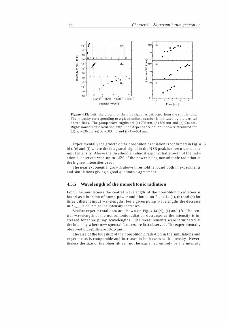
44 Chapter 4. Supercontinuum generation
Figure 4.13: Left: the growth of the blue signal as extracted from the simulations.The intensity corresponding to a given soliton number is indicated by the verticaldotted lines. The pump wavelengths are (a) 780 nm, (b) 836 nm and (c) 934 nm.Right: nonsolitonic radiation amplitude dependence on input power measured for(d) λP =836 nm, (e) λP =883 nm and (f) λP =934 nm.
Experimentally the growth of the nonsolitonic radiation is confirmed in Fig. 4.13(d), (e) and (f) where the integrated signal in the NSR peak is shown versus theinput intensity. Above the threshold an almost exponential growth of the radi-ation is observed with up to ∼5% of the power being nonsolitonic radiation atthe highest intensities used.
The near exponential growth above threshold is found both in experimentsand simulations giving a good qualitative agreement.
4.5.5 Wavelength of the nonsolitonic radiation
From the simulations the central wavelength of the nonsolitonic radiation isfound as a function of pump power and plotted on Fig. 4.14 (a), (b) and (c) forthree different input wavelengths. For a given pump wavelengths the decreasein λNSR is 3-9 nm as the intensity increases.
Similar experimental data are shown on Fig. 4.14 (d), (e) and (f). The cen-tral wavelength of the nonsolitonic radiation decreases as the intensity is in-creased for three pump wavelengths. The measurements were terminated atthe intensity where new spectral features are first observed. The experimentallyobserved blueshifts are 10-15 nm.
The size of the blueshift of the nonsolitonic radiation in the simulations andexperiments is comparable and increases in both cases with intensity. Never-theless the size of the blueshift can not be explained entirely by the intensity

4.5 Comparison with experiments 45
Figure 4.14: Left: the blueshift of the nonsolitonic radiation as extracted from thesimulations. The intensity corresponding to a given soliton number is indicatedby the vertical dotted lines. The pump wavelengths are (a) 780 nm, (b) 836 nmand (c) 934 nm. Right: experimentally measured nonsolitonic radiation wavelengthdependence on input power (d) λP =836 nm, (e) λP =883 nm and (f) λP =934 nm.
dependent term in the phase-matching condition in Eq. (4.3) (a three-fold in-crease in intensity only shifts the phase-matched wavelength by ∼1nm ). Ratherit is the change of the pulse itself due to third-order dispersion, self-phase mod-ulation and Raman scattering that changes the matching conditions betweenthe evolving pump pulse and the nonsolitonic radiation. It was found that theinclusion of the nonlinear effects in Eq. (3.32) as compared to a Kerr type nonlin-earity (∝ |A|2A) gives a larger blueshift when the intensity is increased. In theprocess of soliton break-up Raman scattering will redshift the input pulse andconsequently the phase-matching condition will be fulfilled for nonsolitonic ra-diation that is more blueshifted.
Furthermore it was found that by increasing the third order dispersion theblueshift is increased to what is experimentally observed. Hence our calcula-tions show that the discrepancy between simulated and experimentally mea-sured blueshift is caused by the differences in the dispersion between the exper-imental and the simulated fiber.
Returning to Fig. 4.12 (a) the simulation points are seen to lie slightly be-low the phase-matching curve. The tendency becomes more pronounced withlarger distance to the zero dispersion wavelength because higher intensity isneeded to broaden the spectrum through self-phase modulation, consequentlythe NSR is blueshifted in agreement with the intensity dependent blueshift seenon Fig. 4.13.

46 Chapter 4. Supercontinuum generation
4.6 Conclusion
The processes initiating supercontinuum formation are governed by formationof (higher-order) solitons. During the evolution of the pump pulse into one orseveral stable solitons, the surplus light is emitted as a dispersive wave. Thesimulations show that a large fraction of the dispersive wave is emitted arounda distinct wavelength if the input intensity is high enough for self-phase modu-lation to broaden the spectrum to the phase-matched wavelength. Investigationof the implications of change in pump wavelength and intensity yielded goodqualitative agreement between experiments and simulations.

C H A P T E R 5Four wave mixing in a
photonic crystal fiber
Supercontinuum generation in a PCF with two zero dispersion wavelengthsis investigated. The special dispersion of the fiber has a profound influenceon the supercontinuum which is generated through self-phase modulation andphasematched four-wave mixing and not soliton fission as in the type of PCFinvestigated in Chap. 4. The supercontinuum has high spectral density andis extremely independent of the input pulse over a wide range of input pulseparameters. Simulations show that the supercontinuum can be compressed toultrashort pulses. This chapter is based on paper [IV].
47

48 Chapter 5. Four wave mixing in a photonic crystal fiber
5.1 Introduction
The anomalous dispersion needed to generate broad spectra through soliton fis-sion [49] makes the supercontinuum generation very susceptible to noise in theinput pulse as noise is amplified through modulation instabilities [80]. The in-terplay between the various nonlinear effects gives rise to temporal and spectralstructure, and compression of the spectrally broad fiber output to a few-cyclepulse is thus extremely difficult. Moreover, small changes in the input pulseparameters can lead to very different output spectra, making the selection of anoptimum fiber for a given application difficult.
In this chapter it will be argued, based on simulations and experiments, thatsupercontinuum generation in a highly nonlinear PCF with two closely lyingzero dispersion wavelengths solves the problems discussed above. In such afiber stable, compressible spectra with high spectral density can be generatedand the spectra are only weakly dependent on the input pulse parameters.
5.2 PCF with two zero dispersion wavelengths
A scanning electron micrograph image of the PCF with two zero dispersionwavelengths is shown in Fig. 5.1. The pitch of the fiber is 0.98 µm and it hasa relative holesize of 0.54. The fiber core diameter is 1.5 µm with a correspond-ing effective area of ∼1.3 µm2 and a high nonlinear coefficent γ of 0.15 W−1m−1.The numerical aperture of the fiber is 0.49 at 800 nm and the fiber is single modebut not polarization maintaining.
10 µm
Figure 5.1: A scanning electron micrograph image of the central region of the fibercross section.
The dispersion of the fiber has been measured using white light interferom-etry [57]. The result of the dispersion measurement is shown in Fig. 5.2 (a).The dispersion properties of the fiber are highly unusual with two closely lyingzero dispersion wavelengths at 780 nm and 945 nm and anomalous dispersion

5.2 PCF with two zero dispersion wavelengths 49
in the narrow range between the two zero dispersion wavelengths. The disper-sion profile should be compared to the dispersion of standard highly nonlin-ear PCFs which have only one zero dispersion wavelength in the visible/near-infrared range and anomalous dispersion at wavelengths above the zero disper-sion wavelength. A number of PCFs exhibit a second but widely separated zerodispersion wavelength at wavelengths typically above 1400 nm.
700 800 900 1000 1100−100
0
100
200
300
400
500
λ [nm]
β 2 [fs
2 /cm
]
(a)
750 800 850 900 950
600
700
800
900
1000
1100
1200
λP [nm]
λ S a
nd
λI [
nm
]
(b)
Figure 5.2: (a) Dispersion properties of the PCF with zero dispersion at 780 nm and945 nm. (b) Phase-matching curves for four-wave mixing in the fiber. Full curve:phase-matching without power-dependent term. Dashed curve: phase-matchingwith an input power of 300 W.
The condition for degenerate phase-matched FWM in the PCF was presentedin Sec. 4.3.6 and as any of the other nonlinear processes in the PCFs the phase-matching is highly depending on the dispersion profile of the fiber. Equation4.7 was solved based on the measured dispersion β2(ω) and the phasematchingconditions shown in Fig. 5.2 (b) were found. The result (full line) is that phase-matching can be obtained for all pump wavelengths in the range in-betweenthe two zero dispersion wavelengths. This is in sharp contrast to the results forPCFs with only one zero dispersion wavelength where phasematching is onlypossible for pump wavelengths below the zero dispersion wavelength [28, 44].In fibers with one zero dispersion wavelength, phasematched four-wave mixingfor pump wavelengths above the zero dispersion wavelength can be obtained byinclusion of a nonlinear phaseshift [28, 44] but in the present fiber phasematch-ing is present at vanishing intensity. When self-phase and cross-phase modu-lation is included in the calculations the phasematching curve splits into twosets of phasematched wavelengths as shown by the dashed curve in Fig. 5.2 (b).The power induced splitting has the benefit of providing phasematched wave-lengths in immediate vicinity of the pump wavelength. For increased intensitythe phasematching curves shrink and for intensities higher than approximately1 kW phasematching is no longer possible.

50 Chapter 5. Four wave mixing in a photonic crystal fiber
5.3 Experiments
Experimental investigations were carried out by the members of the Femto Chem-istry Laboratory. Light from a standard Ti:sapphire femtosecond laser was cou-pled into a 50 mm long piece of the PCF with a standard 60× microscope objec-tive. An input coupling efficiency of up to 50% was obtained. The input inten-sity to the fiber is adjusted with a λ/2 plate and a polarizer. The light emanatingfrom the PCF is butt-coupled to a standard fiber connected to an spectrum ana-lyzer where spectra are recorded as the input pulse parameters are varied.
The major experimental findings are shown in Fig. 5.3 (a) and Fig. 5.4 (a) withall spectra plotted on a linear scale. In the first experiment a 40 fs pulse centeredat 790 nm is launched into the fiber and the spectral evolution is followed asthe input pulse energy is increased. At low pulse energies a fast broadening ofthe spectrum is observed, but as the pulse energy is increased above ∼100 pJthe spectral broadening enters a saturation regime where the output spectra areremarkably similar as the pulse energy is increased. Indeed, the supercontin-uum is characterized by two peaks with fixed, sharp inner edges at ∼740 nmand ∼950 nm and two outer edges which slowly move outward with increasingpulse energy. Above the threshold an almost complete depletion of power in theregion between 740 nm and 950 nm is measured and more than 99% of the lightemanating from the fiber is contained in the two spectral peaks. In Fig. 5.4 (a)
Wav
elen
gth
[n
m]
(a)
0.2 0.4 0.6 0.8 1
600
800
1000
1200
1400
Energy [nJ]
(b)
0.2 0.4 0.6 0.8 1
600
800
1000
1200
1400
0
0.2
0.4
0.6
0.8
1
Figure 5.3: (a) Experimental measurement of output spectra versus pulse energyfor a 40 fs input pulse centered at 790 nm. (b) Theoretical simulation of the spectralevolution.
the spectral output for 3 different femtosecond pulses are shown and the cen-tral wavelength and pulse chirp have been varied, while the pulse energy hasbeen kept constant. Irrespective of the input pulse wavelength and chirp almostidentical spectra with depletion of power in the region between ∼740 nm and∼950 nm are obtained. For all pump wavelengths and durations, identical be-haviour with increasing pulse energy was observed, i.e. above the threshold the

5.4 Pulse evolution in the fiber 51
600 800 1000 1200 14000
0.2
0.4
0.6
0.8
1
Inte
nsi
ty [
a.u
.]
(a)
600 800 1000 1200 14000
0.2
0.4
0.6
0.8
1(b)
600 800 1000 1200 14000
0.2
0.4
0.6
0.8
1
Wavelength [nm]
Inte
nsi
ty [
a.u
.]
(c)
600 800 1000 1200 14000
0.2
0.4
0.6
0.8
1
Wavelength [nm]
(d)
Figure 5.4: (a) Experimentally recorded output spectra 40 fs, λ0=790 nm (black),40 fs, λ0=810 nm (red) and a 40 fs, λ0=790 nm chirped to ∼80 fs (blue). The pulse en-ergy is 700 pJ for all pulses. (b) Simulated spectra for λ0=790 nm (black), λ0=700 nm(red) and λ0=1000 nm (blue). For all pulses the energy is 700 pJ and they are 40 fslong. (c) Simulated spectra for 40 fs, 700 pJ (black), 20 fs, 350 pJ (red) and 160 fs,2800 pJ (blue). For all pulses λ0=790 nm. (d) Simulated spectra for an unchirped40 fs pulse (black), upchirped to 80 fs (red) and downchirped to 80 fs (blue) pulses.For all pulses the energy is 700 pJ, λ0=790 nm.
output consists of two peaks with fixed, sharp inner edges and slowly outwardmoving outer edges.
5.4 Pulse evolution in the fiber
The pulse evolution in the PCF is modelled with Eq. (3.32) and intuitive imagesof the pulse evolution are obtained by plotting the time-wavelength distribu-tions S(z, t, λ) defined in Eq. (4.8) with α =100 fs.
Figure 5.5 (a)-(f) show spectrograms of a 40 fs pulse centered at 790 nm asit propagates through the fiber with a pulse energy of 700 pJ. Once launchedin the fiber, the pulse spectrum begins to broaden due to self-phase modula-

52 Chapter 5. Four wave mixing in a photonic crystal fiber
tion. After a few mm of propagation the spectrum breaks into two major peaks.Upon further propagation the two major peaks move outward from the origi-nal pump wavelength while a steadily increasing number of sub-peaks developin-between the two major peaks. After approximately 2 cm of propagation theouter edges of the spectrum reach their final values and the number of sub-peaks increases no further. Upon further propagation the intensity is foundto redistribute within the spectrum. In particular the region between 770 nmand 980 nm is depleted in excellent agreement with the experimental observa-tion. During the propagation the major peaks are influenced by the dispersionof the fiber as seen from the bending of the major peaks in the spectrogram. Thesimulated spectra extend further into the infrared region than the experimentalspectra. This discrepancy is explained by leakage losses of the present fiber atwavelengths above 1100 nm.
These supercontinuum results are in marked contrast to what was observedin the previous chapter for standard PCFs with only one zero dispersion wave-length or two widely separated zero dispersion wavelengths. The fission ofsolitons for the standard fibers is known to create excess noise in the supercon-tinuum due to modulation instability gain which amplifies noise in the inputpulse [80].
In the present fiber, self-phase modulation broadens the spectrum and herebyprovides seed wavelengths for degenerate and non-degenerate four-wave mix-ing. Initially the intensity is too high to provide phasematching but as soon thethe intensity is low enough four-wave mixing proceeds effectively. Because thefour-wave mixing process can be phasematched for low intensities, it becomesthe dominant mechanism whereas soliton dynamics is arrested and plays onlya minor role in the formation of the supercontinuum.
In the absence of soliton fission the supercontinuum is expected to containless noise than supercontinua from conventional PCFs. Experimentally the am-plitude noise across the optical spectrum has been measured. Using a grat-ing and a slit the supercontinuum was spectrally divided into 2 nm slots andthen detected by a fast Si photo diode. The resulting photo diode voltage wasFourier-analysed by a frequency analyser in the range 0-80 MHz. For each 2 nmslot the signal power at 76 MHz was compared to the maximum noise featurein the spectrum. The spectra were however seen to be flat and without noiseover the entire frequency range. In conclusion only an upper limit of the noisecould be established. The optical spectrum in the range 600 nm to 700 nm wasanalysed in this manner and the noise level was found to be at least 60 dB belowthe signal power at all wavelengths. Consequently the supercontinuum fromthis fiber contains less noise than previously reported supercontinua in whichsignificant white noise was present [36]. It should be noted that in the presentexperiment and in the experiments reported in [36] it was not possible to mea-sure the noise on the laser, only an upper limit was established.
Both experimentally and theoretically the spectral depletion extends outsidethe region for phasematched degenerate four-wave mixing given by the twozero dispersion wavelengths Fig. 5.2. The additional depletion is caused by

5.4 Pulse evolution in the fiber 53
(a)
−1 0 1
600
800
1000
1200
1400 (b)
−1 0 1
600
800
1000
1200
1400
Wav
elen
gth
[n
m]
(c)
−1 0 1
600
800
1000
1200
1400 (d)
−1 0 1
600
800
1000
1200
1400
(e)
−1 0 1
600
800
1000
1200
1400 (f)
−1 0 1
600
800
1000
1200
1400
[a.u.]
Time [ps]
0 0.2 0.4 0.6 0.8 1
Figure 5.5: (a)-(f) Calculated spectrograms after propagation of (a) 0 cm, (b) 0.2 cm,(c) 0.5 cm, (d) 1 cm, (e) 2 cm and (f) 5 cm in the fiber for a 40 fs input pulse at 790 nmwith a pulse energy of 700 pJ.

54 Chapter 5. Four wave mixing in a photonic crystal fiber
non-degenerate four-wave mixing being phasematched for a broader range ofwavelengths. The reversed non-degenerate four-wave mixing process movingenergy back into the depleted region is suppressed, due to group velocity walk-off.
This understanding of the supercontinuum generation process in the fiberis confirmed by simulations where the dispersion of the fiber has been shiftedβ2(ω) → β2(ω) + β′, so the fiber has normal dispersion for all wavelengths. Theshift of β2(ω) removes the possibility of phasematched degenerate four-wavemixing, and with this channel closed only a minor depletion of the intensity be-tween 770 nm and 980 nm is found. It is therefore concluded that phasematchedfour-wave mixing is the main cause of the intensity depletion between 770 nmand 980 nm. In the simulations with the shifted dispersion, formation of sub-peaks in the 770 nm to 980 nm region is still observed, but the substructure isremoved if β2(ω) is shifted even further into the normal dispersion regime. Theshifting reduces the influence of higher-order dispersion and it is concluded thatthe interplay between self-phase modulation and higher-order dispersion is thecause of the sub-structure.
Simulations using a standard nonlinear Schrodinger equation (3.34) werealso performed, where higher-order nonlinear effects, i.e., Raman scattering andself-steepening were omitted in Eq. (3.32) and minor differences in the outputwas found. This result originates in the threshold pump power for Raman scat-tering being higher than the threshold for four-wave mixing if phasematchingis achieved [41]. The fact that four-wave mixing supersedes Raman scatteringresults in a higher output power of the field as no energy is lost to phonons inthe fiber. Spectral and temporal effects originating in self-steepening are effec-tively superseded by phasematched four-wave mixing. From the simulations itis concluded that the influence of higher-order nonlinear effects are suppresseddue to the phasematching of four-wave mixing.
Figure 5.3 (b) shows a simulation of the power dependence of the spectralevolution using the nonlinear Schrodinger equation (3.34) with input pulse pa-rameters identical to what is used in Fig. 5.3 (a) that is a 40 fs pulse centeredat 790 nm. The experiment and simulation are in almost complete agreementand the overall shape is extremely well reproduced. Leakage losses at wave-lengths above 1100 nm again cause the simulated spectra to extend further intothe infrared region than the experimental spectra. The mean photon numberis conserved after 5.0 cm of propagation within the numerical accuracy of thesimulations presented in this chapter. The simulated threshold for depletion ofthe 770 nm to 980 nm region is at ∼50 pJ pulseenergy which is lower than theexperimentally observed value of ∼100 pJ. This discrepancy is attributed to thelack of polarization maintenance in the fiber. The differences in the substruc-ture between experiments and simulations can also be ascribed to the lack ofpolarization maintenance not accounted for in the simulation, in combinationwith the lower resolution in power in the experiment. Polarization maintainingfibers with similar dispersion have been produced after this work was done.
In Fig. 5.4 (b)-(d) the fiber output for a variety of pulses is shown. The sim-

5.4 Pulse evolution in the fiber 55
ulations allow the usage of a greater span of pulses than experimentally avail-able. In Fig. 5.4 (b) the central wavelength of the 40 fs input pulse is varied from700 nm to 1000 nm. The generated spectra consist of two major peaks locatedoutside the depleted region, which extends from 770 nm to 980 nm regardlessof the pump wavelength. Using a blueshifted pump wavelength the energycontent of the blue peak is enhanced and vice versa. The double peaked spec-trum is obtained with pump wavelengths spanning from below 600 nm to above1200 nm. Figure 5.4 (c) shows the outcome when the pulse duration is changedfrom 20 fs to 160 fs while keeping the peak intensity fixed. Again, very similarspectra consisting of two peaks with a fixed, strongly depleted region in be-tween the peaks are observed. For pulse durations above ∼500 fs the formationof the double peaked spectrum stops. This change is due to insufficient self-phase modulation for long pulse durations i.e. the spectrum does not broadenenough to provide seed wavelengths for the four-wave mixing. Finally, Fig. 5.4(d) shows simulations where the 40 fs input pulse has been up- or down-chirpedto a pulse duration of 80 fs. As is evident from the figure the supercontinuum isonly weakly dependent on the chirp of the input pulses.
In a fiber with a single zero dispersion wavelength phase-matched four-wave mixing can assist in generating a depleted region in the output spectrum.In that case the different phasematching condition is responsible for a depletionaround the zero dispersion wavelength, and the fiber has to be pumped nearthe zero dispersion wavelength for the conversion to work [81, 82]. In contrastthe present fiber can be pumped anywhere in between the two zero dispersionwavelengths with high conversion efficiency and it is the region between thezero dispersion wavelengths that is depleted.
Figure 5.6 shows a plot of the spectral intensity and phase after 5 cm of prop-agation. The amplitude and phase of the output are smooth as expected fromthe spectrograms. Due to the smooth phase of the single pulse spectrum, theexperimentally realized bandwidth of more than 75 THz in the visible peak cen-tered at 640 nm is therefore compressible to a sub-10 fs pulse. Due to the leakageloss the experimentally realized bandwidth is only ∼30 THz in the near-infraredpeak, which can sustain a 15 fs pulse. Pulse compression has been demonstratedin PCFs with a single zero dispersion wavelength [83], but the compressabilitywas limited by the soliton fission and resulting breakup of the spectrum.
A theory, not relying on the slowly varying envelope approximation, of fourwave mixing in PCFs in the continuous wave regime was presented in [84].The possibility for phase-matched FWM was predicted for PCFs with two dis-tant zero dispersion wavelengths. This FWM was not experimentally observedwhen the fibers were pumped with femtosecond pulses, since the zero disper-sion wavelengths were too distant to make SPM broaden the spectrum enoughto seed the FWM.

56 Chapter 5. Four wave mixing in a photonic crystal fiber
600 800 1000 1200 14000
1000
2000
Ph
ase
[rad
]
Wavelength [nm]
← →
600 800 1000 1200 14000
0.5
1
Inte
nsi
ty [
a.u
.]
Figure 5.6: Spectrum (black) and phase (red) of the pulse after 5 cm for the 40 fsinput pulse at 790 nm with a pulse energy of 700 pJ (also pictured in Fig. 5.5 (f)).The phase of the pulse is well behaved and the visible peak in the spectrum cansustain a sub-10 fs pulse with λ0=640 nm.
5.4.1 Computational methods
All simulations presented in this chapter are computed with method B pre-sented in Sec. 3.6, whereas method A was used for the simulations in the as-sociated article [IV]. Spectra calculated with method A and B are compared inFig. 5.7. Unfortunately, there is an observable difference for the short pulsesused in this chapter, mainly due to the implementation of the self-steepeningterm in method A, where only two points are used to calculate the time deriva-tive. Consequently, method B is the most exact.
600 800 1000 1200 14000
0.2
0.4
0.6
0.8
1
Wavelength [nm]
Inte
nsi
ty [
a.u
.]
Figure 5.7: Full line: This spectrum is computed with method B described in Sec. 3.6and is identical to the spectrum shown in Fig. 5.6. Dashed line: The spectrum com-puted with method A.

5.5 Applications 57
5.5 Applications
Computer simulations show that the spectral position of the major peaks can betuned by tuning of the two zero dispersion wavelengths. Using a set of carefullydesigned PCFs short pulse generation throughout most of the visible and near-infrared region is therefore possible. Such tunable pulses are applicable in e.g.two color high repetition rate time-resolved pump-probe spectroscopy.
The possibility to generate a stable, compressible supercontinuum with highspectral density leads to a number of improvements in the applications of su-percontinua. An advantage in frequency metrology is that the spectral densityat ω and 2ω can be optimized by using a fiber with two properly chosen zero dis-persion wavelengths. Moreover, the smaller noise present in a supercontinuumgenerated through phasematched four-wave mixing can increase the signal tonoise ratio in experiments, e.g., in fiber based CARS microscopy [II]. Similarlythe supercontinuum provides easy access to new wavelength regions for two-and three-photon microscopy [85]. In addition, the dominating FWM could beuseful for the production of frequency-converters for optical networks.
5.6 Phase-matched FWM - continuous wave regime
In the Femto Chemistry Laboratory it was found that phase-matched four wavemixing is significant as well in the CW regime for a similar fiber with dispersionprofile β2(ω) shown in Fig. 5.8 (a). The condition for phase-matching of degen-erate FWM is again given by Eq. (4.7) and the solution to the equation is shownin Fig. 5.8 (b) for powers of 0 W and 1000 W. In the CW regime the influenceof the power on the phase-matching condition is very limited. There is a signif-icant extra bend in the 0 W phase-matching curve on Fig. 5.8 (b) as comparedto Fig. 5.2 (b) due to opposite signs between the determining higher order evendispersive terms [V].
The experimental demonstration of the FWM in the fiber is shown in Fig. 5.9.Part (a) of the figure shows experimental data for the FWM on the major axis andpart (b) shows experimental data on the minor axis. The discrepancy betweenthe measurements and the calculated phase-matching curve originates in themeasurement of the dispersion, which was not done for the polarization direc-tions separately. Due to the bend on the phase-matching curve it is possible togenerate signal light in the whole wavelength range between 500 and 650 nm,giving perspectives for a source of green or blue light.
5.7 Conclusion
In summary, a new way of generating a stable and intense supercontinuumthrough self-phase modulation and phasematched four-wave mixing in a newlydesigned PCF with two closely lying zero dispersion wavelengths has been

58 Chapter 5. Four wave mixing in a photonic crystal fiber
600 800 1000 1200 1400 1600−500
0
500
1000
1500
2000
2500
Wavelength (nm)
β 2 (fs
2 /cm
)
(a)
600 800 1000 1200 1400400
600
800
1000
1200
1400
1600
1800
Pump Wavelength (nm)
Pha
sem
atch
ed W
avel
engt
s (n
m) ***** P = 0 W
___ P = 1000 W (b)
Figure 5.8: (a) β2 for the used PCF with two zero dispersion wavelengths. (b) Condi-tion for degenerate phase-matched FWM in the fiber with pump powers of 0W and1000W . The figures are from the article [V] made by Thomas Vestergaard Andersen.
740 750 760 770 780 790400
600
800
1000
1200
1400
1600
1800Major axis
Pump Wavelength (nm)
Pha
sem
atch
ed W
avel
engt
hs (
nm)
λ0 λ
0
1064/766/598nm
(a)
740 750 760 770 780 790400
600
800
1000
1200
1400
1600
1800Minor axis
Pump Wavelength (nm)
Pha
sem
atch
ed W
avel
engt
hs (
nm)
1064/749/578nm
λ0
(b)
Figure 5.9: (a) Experimental data for the FWM on the major axis. (b) Experimentaldata for the FWM on the minor axis. The figures are from the article [V] made byThomas Vestergaard Andersen.
demonstrated. Standard supercontinuum generation in PCFs relies on anom-alous dispersion and the supercontinuum generated through soliton fission be-comes very susceptible to the characteristics of the input pulse as noise is am-plified through modulation instabilities. However, in the present PCF both thesoliton fission mechanism and the noise amplification though modulation insta-bilities are suppressed. Consequently, both the amplitude and the phase of thesupercontinuum are well-behaved, and extremely unsusceptible to the characterof the input pulse. By optimizing the dispersion profile of the double zero dis-persion wavelength fibers the generated stable supercontinuum can be tailoredfor the many applications envisaged, in particular compression to ultrashortpulses, metrology, pump-probe spectroscopy and non-linear microscopy.

C H A P T E R 6Introduction to
Bose-Einstein condensatesin optical lattices
In this chapter, an introduction to the field of BEC physics will be given withemphasis on condensates in periodic potentials. A derivation of the Gross-Pitaevskii equation will be sketched, the equivalent equation in nonlinear atomoptics to the nonlinear Schrodinger equation in nonlinear optics. More thoroughintroductions to BEC physics are given in the books by Pethick and Smith [86],Pitaevskii and Stringari [87] and the review articles [88–90]. Recently excellentreviews on BEC physics in optical lattices have been written [91, 92].
59

60 Chapter 6. BEC in optical lattices
6.1 Introduction
In the process of Bose-Einstein condensation where a single quantum state ismacroscopically occupied, the boson nature of the particles is clearly revealed.Since the initial realizations of Bose-Einstein condensation in 1995 [1, 2, 93] ahuge research effort has been put into the field, both regarding theory and ex-periments. The 2001 Nobel prize in Physics was awarded to Cornell, Wieman[94] and Ketterle [95] for their achievements of BEC. A typical realization ofa BEC relies on laser cooling of the atomic gas in a magneto-optical trap andsubsequent evaporative cooling in a conservative trap. A review of experimen-tal techniques is given in [96]. The laser cooling of atoms, being a major stepon the road to BEC, lead to the 1997 Nobel prize in physics awarded to Chu,Cohen-Tannoudji and Phillips. After the successful applications of the lasersfor the near resonant Doppler and Sisyphus cooling processes the next step wasfar detuned optical lattices forming conservative periodic potentials seen by thecondensates.
Two amazing branches of physics are united in the system of a BEC in anoptical lattice and the system is literally tunable. Through a Feshbach resonancethe sign and magnitude of the nonlinear interaction can be tuned through the s-wave scattering length of the condensate. Simultaneously the optical lattice canbe tuned forming perfectly periodic 1D, 2D or 3D spatial structures changingthe periodicity of the BEC. The tunability of the periodicity offers a degree offreedom, unavailable in traditional condensed matter systems of electrons in acrystal lattice, where the periodicity is given by the material.
Photonic crystals and PCFs are revolutionizing technologies exactly becausethey provide a micro-structuring and thereby a periodicity in one, two or threedimensions. The periodicity can be manipulated and designed after almost anywish. Still, the optical lattice offers a tunability of the periodicity to the BECduring an experiment. The photonic crystal on the other hand has its final shapeafter it has been manufactured, and consequently it does not offer this tunabilityduring an experiment.
The huge flexibility of the system of the BEC in the optical lattice has a price.It is a complicated experiment to conduct, indeed more complex than most ex-periments on the fundamental physics in photonic crystals, where most oftenno vacuum chambers are needed. Still, it is worth the effort. A lot of condensedmatter physics can be investigated in BECs in optical lattices. Certainly, the na-ture of superfluidity can be investigated in the very clean system provided bythe BEC, where almost the entire atomic cloud can be condensed into the super-fluid phase. Strong correlations in a many body quantum mechanical systemare elucidated in the Mott insulator transition, illustrating the Heisenberg un-certainty of the phase and the number of atoms. Recently, the Mott insulatorstate was demonstrated in Munich [97] bringing much attention to the field.Many quantum statistical phenomena can be investigated. Huge possibilitiesare related to investigating Fermi gases alone or together with Bose gases in op-

6.2 Fundamentals of BEC physics 61
tical lattices [98]. The field of quantum information processing could benefit,for instance by using the Mott insulator state for a natural quantum register, assuggested in Ref. [92].
Finally, a lot of the physics learned in nonlinear optics can be directly trans-ferred to the BEC system with the periodic potential. For example the ap-proaches to investigations of bright solitons in cold atomic gases were greatlyinfluenced by nonlinear optics [99], where a multiple scales analysis carried outin optics could be almost directly translated [100, 101]. Russell and coworkers[102] used their knowledge from fiber optics about the generation of nonsoli-tonic radiation and the breakup of solitons in PCFs to investigate the breakupof gap solitons in BECs in periodic potentials. The FWM process investigated inChap. 7 is indeed inspired by the phase-matched FWM playing a central role inthe light propagation in the PCF.
The fields of nonlinear atom optics and nonlinear optics have a common ori-gin, since the systems investigated in the two fields can basically be described bythe Maxwell-Bloch equations. In the case of nonlinear optics the atomic degreesof freedom have been eliminated only preserving a linear and nonlinear suscep-tibility of the medium leading to an effective equation for the electromagneticfield only, the nonlinear Schrodinger equation derived in Chap. 3. In nonlinearatom optics an opposite procedure can be used. By eliminating the light fieldfrom the Maxwell-Bloch equations a nonlinear master equation for the atomscan be derived [103]. If dissipation is insignificant the master equation can bereduced to a nonlinear Schrodinger equation, but this time for the atomic field(the Gross-Pitaevskii equation) [103]. In the present chapter the Gross-Pitaevskiiequation will be derived using the standard approach, by constructing an equa-tion for N identical particles and subsequently making a mean-field approxima-tion.
6.2 Fundamentals of BEC physics
To describe the physics of a BEC, a system of N identical, interacting bosonsmoving in three dimensional space and potentially subjected to external forceswill be considered. The bosons can be described by a many-body wave functionΦ(r1, r2, ..., rN , t) and the time evolution can be found by solving the many-body Schrodinger equation
i∂
∂tΦ(r1, r2, ..., rN , t) = HΦ(r1, r2, ..., rN , t), (6.1)
on the premise that the initial state of the system is known. The Hamiltonian Hcontains single particle Hamiltonians given by
h(r) = − 2
2m∇2 + Vext(r), (6.2)
where Vext(r) is the external potential and m is the mass of an atom. Underthe assumption of a dilute gas, third and higher order interaction terms can be

62 Chapter 6. BEC in optical lattices
neglected and only two-body terms V (rj , rk) are needed to describe the inter-actions. The complete microscopic information about forces and interactionsworking on the bosonic particles is consequently contained in the Hamiltonian
H =N∑
j=1
h(rj) +N∑
j,k=1, j<k
V (rj , rk). (6.3)
6.2.1 The two-body interaction potential
For alkali atoms the structure of the actual interaction potential is quite com-plicated, having a repulsive hard core and many bound states. As mentionedabove the bosonic gas is assumed to be dilute. The requirement for a gas withdensity ρ to be dilute is that the average distance between atoms ρ−1/3 is muchlarger than the range of the potential. Finding more than two particles at thesame point in space is very unlikely, when the gas is dilute. Consequently, thirdand higher order interaction terms can be neglected as mentioned above. Thetwo body interaction only depends on the distance between the particles, noton the actual positions of the particles, i.e. V (r, r′)=V (r − r′). Additionally, thedetails of the scattering potential do not matter, since the particles do not getclose enough to probe the details of the potential. If furthermore the tempera-ture is low, the scattering takes place in the s-wave only, the scattering is fullyelastic and the scattering potential can be substituted with a zero range pseudo-potential
V (r − r′) = gδ(r − r′), (6.4)
where g is the so-called coupling constant,
g =4π
2
mas. (6.5)
The pseudo-potential is consequently fully characterized by the s-wave scatter-ing length as of the exact potential and as can be experimentally measured. Re-pulsive atom-atom interactions are characterized by a positive scattering length,which is the case in the proposal presented in Chap. 7. For a negative scatteringlength the atom-atom interaction is attractive. Above a certain number of atomsthe condensate collapses because the kinetic energy is no longer sufficient tokeep the atoms apart, as first experimentally demonstrated in 7Li [93]. The signand magnitude of the scattering length can be tuned by external fields with Fes-hbach resonances [104, 105], making the scattering length a tunable parameterfor the system of the condensate. In atom optics the scattering length plays anequivalent role to the nonlinear susceptibility in nonlinear optics. For a PCF thenonlinear susceptibility is a material specific parameter. Additionally, the mi-cro structuring of the fiber is responsible for the high intensity levels achievablewithin the fibers and the resulting nonlinear effects. Still, that does not make thenonlinear response of the fiber tunable in the sense that the nonlinearity can betuned during an experiment with a single fiber, as opposed to the BEC wherethe Feshbach resonace can be tuned.

6.2 Fundamentals of BEC physics 63
6.2.2 Second quantized Hamiltonian
In the second quantization creation and annihilation operators are introducedfor the bosons. The bosonic field operator ψ†(r) creates a boson at the positionr and ψ(r) annihilates a boson at position r. In the second quantization the fullHamiltonian in Eq. (6.3) is given by
H =∫dr ψ†(r)
[−
2
2m∇2 + Vext(r)
]ψ(r)
+12
∫ ∫dr dr′ ψ†(r)ψ†(r′)V (r, r′)ψ(r)ψ(r′). (6.6)
The pseudo-potential Eq. (6.4) can be inserted above giving the following ex-pression
H =∫dr ψ†(r)
[−
2
2m∇2 + Vext(r)
]ψ(r)
+g
2
∫dr ψ†(r)ψ†(r)ψ(r)ψ(r). (6.7)
This second quantized Hamiltonian will be the starting point for the derivationof the Gross-Pitaevskii equation.
6.2.3 The Bogoliubov approximation and mean field theory
The many body Hamiltonian (6.7) fully describes the behavior of the particles,but in the case of a dilute bose gas mean field theories can describe the systemvery well. It is characterized by a small set of parameters like the condensatewave function and the chemical potential.
In 1947 Bogoliubov [106] described a dilute homogeneous Bose gas with amean field theory, where the condensate contribution to the bosonic field oper-ator is separated out. The field operator can be written as
ψ(r) =∑
k
ψk(r)ak, (6.8)
where ψk(r) is a single particle wave function and a†k, ak are the correspondingbosonic creation, annihilation operators defined in Fock space:
a†k |n0, n1, ..., nk, ...〉 =√nk + 1 |n0, n1, ..., nk + 1, ...〉 (6.9)
ak |n0, n1, ..., nk, ...〉 =√nk |n0, n1, ..., nk − 1, ...〉 (6.10)
and they obey the normal bosonic commutation relations
[ak, a†q] = δk,q, [ak, aq] = 0. (6.11)

64 Chapter 6. BEC in optical lattices
As mentioned, the idea is to separate the bosonic field operator into a condensedpart ψ0(r)a0 and a non-condensed part δψ(r)
ψ(r) = ψ0(r)a0 + δψ(r). (6.12)
For Bose-Einstein condensation to occur, the number of atoms in the lowest ly-ing single particle state must be macroscopic i.e. n0 1 and n0/NT must re-main finite for NT → ∞, where NT is the total number of atoms. The approachof Bogoliubov [106] is based on the following two approximations:
• The operator δψ(r) is treated as a small perturbation, a good approxima-tion if the fraction of non-condensed atoms is small.
• Given that a0|n0, ...〉 =√n0|n0, ...〉 and a†0|n0, ...〉 =
√n0 + 1|n0, ...〉, the
approximation is to replace the operators a0 and a†0 with c-numbers suchthat a0 = a†0 =
√n0, which is reasonable, when the condensed state is
macroscopically occupied.
The resulting expression for the boson field operator in the Bogoliubov approx-imation is the following
ψ(r) =√Nψ(r) + δψ(r), (6.13)
where the number of atoms in the ground state n0 has been replaced with Nand the condensate wave function ψ0(r) with ψ(r). In the following it will beshown that approximating the bosonic field operator with the condensate wavefunction leads to the Gross-Pitaevskii equation.
6.2.4 The Gross-Pitaevskii equation
To derive the Gross-Pitaevskii equation, the second quantized Hamiltonian fromEq. (6.7) is inserted into the Heisenberg equation of motion, resulting in the fol-lowing expression
i∂ψ(r, t)∂t
=[ψ(r, t), H
](6.14)
=[−
2
2m∇2 + Vext(r, t) + gψ†(r, t)ψ(r, t)
]ψ(r, t), (6.15)
where the following bosonic commutation relations for the field operator wereused to reduce the expression
[ψ(r), ψ†(r′)] = δ(r − r′), [ψ(r), ψ(r′)] = [ψ†(r), ψ†(r′)] = 0. (6.16)
Now the Bogoliubov approximation is used and the bosonic field operator issubstituted with ψ(r, t) =
√Nψ(r, t) whereby excitations are completely ne-
glected. The result is
i∂ψ(r, t)∂t
=[−
2
2m∇2 + Vext(r, t) + gN |ψ(r, t)|2
]ψ(r, t), (6.17)

6.2 Fundamentals of BEC physics 65
which is the so called Gross-Pitaevskii equation for the condensate wave func-tion. If the external potential is time independent and the gas is in thermalequilibrium, solutions to the Gross-Pitaevskii equation which are only time-dependent through a global phase can be found. Writing such a solutions as
ψ(r) exp(−iµt), (6.18)
the time independent Gross-Pitaevskii equation appears
[−
2
2m∇2 + Vext(r) + gN |ψ(r)|2
]ψ(r) = µψ(r). (6.19)
In the Gross-Pitaevskii equation the term gN |ψ(r)|2 describes the interactionsof an atom in the condensate with the other N − 1(∼ N for big NT ) atoms inthe condensate, i.e. the atom sees the mean field of the other atoms, but sincethey are all in the same quantum state, the other atoms can be described withthe same single particle wave function ψ(r), normalized to 1. The density of thecondensate is then given by N |ψ(r)|2. The global phase µ in the wave function(6.18) is equal to the chemical potential giving the energy required to add another particle to the condensate. The Gross-Pitaevskii equation can be derived ina number of other ways. One way, illustrating the role of the chemical potential,is to start from the grand canonical many body Hamiltonian K = H − µN ,where the chemical potential µworks as a Lagrange multiplier and the last termsecures the mean number of particles. By inserting ψ =
√Nψ and making a
variation of K with respect to ψ∗ the Gross-Pitaevskii equation is found.The Gross-Pitaevskii equation is the equivalent in nonlinear atom optics to
the nonlinear Schrodinger equation in nonlinear optics. Additionally, the mean-field treatment in atom optics is equivalent to the classical treatment of the elec-tromagnetic field in optics. To go a step further in the analogy, a quantum opticstreatment of the photons with creation an annihilation operators is equivalentto the second quantization in atom optics.
6.2.5 Elementary excitations
Because excitations have been neglected in the derivation, the Gross-Pitaevskiiequation is only valid at T = 0K, and even there it is approximate since theinteractions lead to quantum depletion; consequently some atoms are in excitedstates even at T = 0. But for cold alkali gases (below the critical temperature)it is generally a good approximation to neglect the number of non-condensedatoms N ′ in comparison with N since the quantum depletion is small.
It can be useful to move beyond the mean field approximation and calculatethe elementary excitations of a condensate, both to investigate the dynamicaland the thermodynamical stability of the condensate. A linear stability analysiscan be performed by assuming the excitations to be small oscillations arounda stationary state ψ(r) of the Gross-Pitaevskii equation. One approach is to as-sume solutions to the time dependent Gross-Pitaevskii equation (6.17) of the

66 Chapter 6. BEC in optical lattices
following form
ψ(r, t) = e−i µ
t
[ψ(r) + U(r)e−iωt − V ∗(r)eiωt
]. (6.20)
After keeping terms linear in U(r) and V (r) in Eq. (6.17) and equating termsproportional to e−iωt and eiωt the Bogoliubov-de Gennes equations appear
L(Uk
Vk
)= ωk
(Uk
Vk
), (6.21)
where the matrix operator L is given by
L =( (
h(r) − µ+ 2gN0|ψ(r)|2) −gNψ(r)2
+gN0ψ∗(r)2 −(h(r) − µ+ 2gN |ψ(r)|2)
). (6.22)
The Bogoliubov-de Gennes equations can be derived in various other ways, forinstance by introducing the Bogoliubov approximation ψ(r) =
√Nψ(r) + δψ(r)
in the grand canonical many body Hamiltonian and collecting terms of secondorder in δψ(r).
Because the evolution of the modes behaves as exp(±iωkt), the criterium fordynamical stability is that all the energies in the Bogoliubov spectrum are real.If the energies of all the modes for which 〈Uk|Uk〉 − 〈Vk|Vk〉 = 1 in addition arepositive the condensate is said to be thermodynamically stable. If on the otherhand some of these energies are real and negative the system is said to exhibit aenergetic instability / Landau instability [107]. For the class of modes for which〈Uk|Uk〉 − 〈Vk|Vk〉 = −1 the criterium for energetic stability is that the energiesare real and negative.
6.2.6 One-dimensional nonlinear Schrodinger equation
A quasi one-dimensional situation can be assumed for a BEC in a one-dimensionalperiodic potential if the condensate is confined in a cylindrically symmetrictrap, and the external potential is generally separable. Furthermore, the atom-atom interaction energy should be smaller than the transverse excitation en-ergy, which for a transverse harmonic confinement is given by E⊥ = ω⊥. Thecondensate is assumed to be in the transverse ground state, which for the har-monic confinement is a gaussian. The single particle wave function is written asψ = ψ⊥(x, y)ψ(z), leading to the one-dimensional Gross-Pitaevskii equation
i∂ψ(z, t)∂t
=[−
2
2m∂2
∂z2+ Vext(z) + γ|ψ(z, t)|2
]ψ(z, t). (6.23)
The strength of the nonlinearity is described by the factor
γ =gN
A⊥, (6.24)

6.3 Bose-Einstein condensates in optical lattices 67
where A⊥ = 2π
mω⊥for the gaussian ground state. The criterium of the atom-
atom interaction energy being smaller than the transverse excitation energy canbe expressed as 2asN |ψ(z)|2 < 1. This weak interaction limit corresponds toabout 100 atoms per µm for 87Rb, the alkali gas used in our proposal in thefollowing chapter.
Salasnich et al. [108] have derived a one-dimensional nonpolynomial non-linear Schrodinger equation for a condensate trapped in a transverse harmonicpotential with trapping frequency ω⊥. The derivation is based on a variationalapproach. For the transverse part of the ground state wave function a gaussianansatz is made
φ(x, y, t;σ(z, t))1√
πσ(z, t)exp[−(x2 + y2)/2σ(z, t)2]. (6.25)
The variation of the action functional associated with the 3D Gross-Pitaevskiiequation is performed with respect to the width of the transverse gaussian σ(z, t)and the longitudinal part of the wave function ψ(z, t). The resulting nonpoly-nomial nonlinear Schrodinger equation is given by [108]
i∂ψ(z, t)∂t
=
[−
2
2m∂2
∂z2+ Vext(z) +
gN
A⊥(z, t)|ψ(z, t)|2 (6.26)
+π
2
mA⊥(z, t)+mω2
⊥A⊥(z, t)4π
]ψ(z, t). (6.27)
where A⊥(z, t) is a function of ψ(z, t)
A⊥(z, t) =2π
mω⊥
√1 + 2asN |ψ(z, t)|2. (6.28)
An advantage of the approach is that the influence of the external potentialVext(z) on the density along the z-axis is treated.
6.3 Bose-Einstein condensates in optical lattices
In this section a brief review over some of the work done in the field will begiven. The aim is to give a background for the proposal presented in Chap. 7.
After theoretical suggestions in 1998 [109, 110], strongly detuned lasers wereused to form effectively conservative periodic potentials, and the field of BECsin optical lattices has grown ever since.
6.3.1 The optical lattice
A one-dimensional periodic potential can be generated by two counter-propagatinglaser beams with equal intensity. The origin of the force felt by the atoms is theAC-Stark shift. The oscillating electric field of the light induces an electric dipole

68 Chapter 6. BEC in optical lattices
moment in the atom. It is then the interaction between the electric field E(r, t)and the induced dipole moment that causes an energy shift in the atomic energylevel given by
∆E(r) = −12α(ω)〈E2(r, t)〉, (6.29)
where α is the polarizability of the atomic level and 〈〉 represents a cycle aver-age. Assuming that the frequency of the light ω is red-detuned, i.e. less thanthe atomic resonance frequency, the induced dipole and the electric field of thelight will be in phase, corresponding to α(ω) > 0. The resulting force on theatom is found via minus the gradient of the energy of the atomic energy leveland the force will point in the direction of increasing intensity of the light field.For a transverse Gaussian laser beam a harmonic approximation can be madefor the central part of the beam, leading to a transverse harmonic potential. Alongitudinal periodic potential arises due to the interference of two counter-propagating laserbeams with wavelength λL = 2π/kL and parallel polariza-tions. The transverse harmonic profile multiplied on the periodic potential isnormally ignored leading to a separable potential, harmonic in the radial coor-dinate and periodic in the longitudinal coordinate z. The z-dependent part ofthe potential has a lattice spacing of d = λL/2 and is given by
V (z) = −V0 cos(2kLz), (6.30)
where V0 is usually measured in units of the recoil energy ER ≡ 2k2
L/2m, withm being is the mass of the atom.
By far the most research into BEC in optical lattices has been carried outin 1D, but the formation of optical lattices in two and three dimension can beachieved by adding more laser beams. The most direct extension is to add apair of lasers perpendicular to the first set, creating a 2D lattice. By adding alast pair in the third spatial direction a 3D lattice can be formed. In fact theMott insulator transition was first demonstrated by Greiner et al. [97] in a 3Dlattice. Stoferle et al. [111] used deep lattices along two spatial directions tocreate arrays of tubes. They subsequently realized the Mott insulator transitionin the longitudinal dimension of the tubes.
6.3.2 Linear description
The dynamics of a condensate in an optical lattice is influenced by the followingparameters: The absolute number of atoms, the depth of the periodic poten-tial, the on site interaction energy and the characteristic energy for tunnelingbetween lattice sites.
When the nonlinear interaction energy is small compared with the strengthof the periodic potential, a simple linear band structure provide very valuableresults. The proposal in Chap. 7 is in this regime with a weak periodic potentialof V0 = ER/2.

6.3 Bose-Einstein condensates in optical lattices 69
The band structure of the one-dimensional linear Schrodinger equation withthe periodic potential in Eq. (6.30) can be found using the method listed in al-most any book on solid state physics [112]. Bloch’s theorem in one dimensionstates that the eigen wave-functions can be written as
ψn,k(z) = eiqzun,k(z), (6.31)
where n is referred to as the band index and k is the quasi-momentum (strictlyk is the quasi-momentum). The functions un,k are periodic with the latticespacing d. The eigen wave-functions and the potential can be expressed as aFourier series
ψn,k(z) =∑K
ck−Kei(k−K)z, (6.32)
V (z) = −V0
2eiQz − V0
2e−iQz, (6.33)
where Q = 2kL is a lattice vector and K takes the values of lattice vectors from−sQ to sQ, where s is the number of points in a period of the direct lattice.Consequently the band structure εn,k can be found by solving the following setof 2s+ 1 coupled linear equations
2
2m(k −K)2
ck−K − V0
2ck−K−Q − V0
2ck−K+Q = εn,kck−K , (6.34)
for the quasi-momenta k in the first Brillouin zone.Making a Taylor expansion of the band structure around a given quasi-momentum
k0 reveals useful information about the dispersive properties of a wave packetcentered at k0. As in nonlinear optics the first derivative gives the group veloc-ity vg . The second derivative gives the effective mass meff corresponding to thegroup velocity dispersion β2 in optics.
vg(k0) =1
∂εn(k)∂k
∣∣∣∣k0
, meff(k0) = 2
∂2εn(k)∂2k
∣∣∣∣k0
−1
. (6.35)
To keep the analogy with optics the central part of the first band in the Brillouinzone from k = 0 to the points of diverging meff corresponds to a region of nor-mal dispersion since meff > 0. The regions around the band edges on the otherhand correspond to anomalous dispersion, since meff < 0.
6.3.3 Nonlinear description
Due to the atom-atom interaction in the BEC, the density of the condensate inthe ground state will be modulated with the period of the optical lattice, causinghigh density at potential minima and low density at potential maxima. Conse-quently, in a shallow lattice the presence of the nonlinear interaction causes an

70 Chapter 6. BEC in optical lattices
effective periodic potential with a smaller modulation resulting in smaller bandgaps and higher bandwidths [109].
For a condensate only modulated by the periodic potential, the nonlinearband structure is given by the chemical potential µ of the time-independentGross-Pitaevskii equation
[−
2
2md2
dz2− V0 cos(2kLz) + γ|ψ(z)|2
]ψ(z) = µψ(z), (6.36)
where γ = gNA⊥
. The chemical potential is equal to the nonlinear eigenvalue.Equivalently to the linear case (6.31), the nonlinear eigenstates ψ(z) = eikzuk(z)can be written on the Bloch form. As in the linear case uk(z), is periodic withthe lattice and k represents wave vectors in the first Brillouin zone.
The Bloch waves uk(z) can be found numerically in various ways [113, 114].In the method applied in [113], uk is expanded in a Fourier series and the Hamil-tonian corresponding to the Gross-Pitaevskii equation (6.36) is minimized in thespace spanned by the Fourier coefficients.
For small nonlinearities the band structure much resembles the band struc-ture of a less deep periodic potential, but when the nonlinearity is considerable,the band structure is significantly altered. When the nonlinear energy becomesgreater than the energy of the band gap, loops (also called swallow tails) appearin the lower band at any band edge in the structure [115]. The indication ofloops was first reported in [116].
6.3.4 General stability properties
It is the presence of the periodicity together with the nonlinearity that opensthe possibility for instabilities. A stability analysis is typically based on a linearexitation around an eigen state of the Gross-Pitaevskii equation leading to theBogoliubov-de Gennes equations as explained in Sec. 6.2.5.
The stability properties are relevant since q states over major parts of theBrillouin zone will be treated in Chap. 7. The occurrence of Landau and dynam-ical instabilities has been investigated by Wu and Niu [113, 114]. The centralpart of the Brillouin zone is energetically and dynamically stable. Moving awayfrom the center there is a region of Landau instability beyond which there is adynamically unstable region until the edge of the Brillouin zone. In general thesmallest region of dynamical instability is found for a shallow lattice and a smallnonlinearity as in our proposal in Chap. 7.
Stationary states with periods equal to multiples of the lattice period havebeen shown to exist [117]. Additionally, a stationary state with the double pe-riod of the lattice is shown to energetically coincide with the dynamical insta-bility at the zone boundary mentioned above. This is very interesting since thedynamical instability is consequently not incoherent in its nature, but could sim-ply indicate a coupling to an other discrete state. This aspect will be treated inChap. 7.

6.3 Bose-Einstein condensates in optical lattices 71
The dynamical instability has recently been experimentally investigated byInguscio and coworkers [118, 119]. After the condensate is generated they adi-abatically turn on an optical lattice generated from two counter propagatinglasers with wavelength around λ and a frequency difference δν. The optical lat-tice is consequently moving with velocity v = (λ/2)δν and the condensate isloaded into a state of well defined quasi-momentum q = mv/. With this exper-imental method, accounted for in detail in [120], the condensate can be givenany desired quasi-momentum. The dynamical instability was experimentallyidentified in [118] by the short lifetime of the condensate in the unstable regime.
Although many experiments are performed outside the weak interactionlimit, only recently the stability analysis has been generalized to include thetransverse degrees of freedom. The thresholds for instabilities are scarcely af-fected by the transverse degrees of freedom, on the other hand the transverseexcitations play an important role inside the regime of dynamical instability,indicated by complex radial dynamics [121].
6.3.5 Shallow lattices
The behavior of the BEC depends on the type of lattice it is situated in. In thissection phenomena typically encountered in a shallow optical lattice will be con-sidered.
Soliton generation, relying on the balancing of nonlinearity and dispersion,can be achieved. The negative effective mass associated with a wave packetat the band gap in an optical lattice can be balanced by repulsive atom-atominteractions leading to a bright gap soliton as experimentally demonstrated in[122]. In the article [I] the stability of these gap solitons was investigated bysolving the Bogoliubov-de Gennes equations.
The fast oscillating scale associated with the lattice can be removed fromthe problem using a multiple scales analysis generalized from optics [100, 101],where it has been used to describe Bragg fibers with a one-dimensional modu-lation of refractive index. The analysis boils down to a nonlinear Schrodingerequation for the soliton envelope function, where the kinetic energy term andthe periodic potential have been replaced by a kinetic energy term with an ef-fective mass.
It should be mentioned that bright solitons can also be generated withoutthe presence of the periodic potential. Bright solitons have been experimentallydemonstrated [123, 124] in condensates of lithium-7 atoms, where the normaldispersion corresponding to the positive mass was balanced by the attractiveinteractions.
A force can be applied to the condensate in the periodic potential, for ex-ample by accelerating the optical lattice potential [125]. Consider a condensatewave packet with a narrow quasi momentum distribution around k0. If the forceis adiabatically applied the condensate will cross the Brillouin zone boundarystaying in the first band. Since the group velocity becomes negative after thezone boundary is crossed, the condensate starts to oscillate in space. These

72 Chapter 6. BEC in optical lattices
so-called Bloch oscillations are discussed in [126], where also the effect of thenonlinearity is discussed.
Landau-Zener tunneling appears if the acceleration is not performed adia-batically, causing the second band to be populated after the zone boundary iscrossed. Experimental studies of the Landau-Zener tunneling effect as well asthe influence of the atom-atom interaction on the effect are reported in [127].The tunneling probability increases due to the interactions. The atoms gatherat the potential wells, leading to a smaller modulation of the effective potentialand hence a smaller band gap and higher tunneling probability [128]. Andersonand Kasevich made a pulsed atom laser in 1998 [129] by coupling atoms out ofthe condensate in a vertical periodic potential. The gravitation was acting as theaccelerating force in this Landau-Zener tunneling process.
6.3.6 Deep lattices
In the case of a deep periodic potential the Bloch states exhibit strong localiza-tion at the lattice sites (the tight binding limit). Consequently, a Wannier basis,where the eigenfunctions are located at the potential minima, can often be moreuseful [130]. The linear Wannier states can be modified to take the effect of theatom-atom interactions into account.
When the number of atoms per lattice site becomes small, the mean fielddescription of the Gross-Pitaevskii equation is no longer fully valid, becausethe particle correlations need to be properly accounted for. Instead, the Bose-Hubbard Hamiltonian was suggested in 1998 [110] for describing the system ofN ultracold atoms confined by the combined potential of a harmonic trap andan optical lattice:
H = −J∑
<ll′>
b†l bl′ +U
2
∑l
nl(nl − 1) +∑
l
εlnl. (6.37)
Here < ll′ > represents the sum over nearest neighbour pairs [131], εl denotesthe energy at site l associated with the harmonic potential, nl is the atom numberoperator and b†l and bl are the boson creation and annihilation operators at site l.Again, the on site interaction energy is denoted U and J is the tunneling energyfrom site to site.
For a shallow lattice the atoms move between adjacent wells due to a smallon site interaction and a high probability for tunneling, corresponding to a smallratio U/J . The condensate has a well determined phase, since each atom issmeared out over the entire lattice and the quantum gas is in the superfluidphase. As the depth of the periodic potential increases the probabitity for tun-neling between adjacent wells becomes very small. The transition to the Mottinsulator phase occurs when the ratio between the on site interaction energy Uand the tunneling energy J from site to site is above a critical value. If the num-ber of lattice wells is assumed equal to the number of atoms, then the interactionenergy associated with placing two atoms at the same site is so big that it is en-ergetically very unfavourable for the system to do it. Consequently, in the Mott

6.4 Conclusion 73
insulator state there is exactly one atom in each well, and the total wave functioncan be written as a product of Fock states for the lattice sites. Since there is nouncertainty in the atom number the phase of the gas is now completely uncer-tain. It should be mentioned that the Mott insulator phase exists for n = 2, 3, 4...atoms per lattice site as well and the critical value of U/J depend on n [131].
6.3.7 Superlattices
A superlattice with a period three times as long as the period of the underlyinglattice has been used by W. D. Phillips and his group to load atoms into everythird lattice site [132]. If atoms in optical lattices shall be used for quantuminformation processing, this is certainly a step forward, since it improves theability to address single atoms.
The introduction of a superlattice, implies the appearance of new gaps inthe band structure of the total system. For a shallow superlattice the introducedgaps will be narrow (mini-gaps), with associated relatively high curvature anddispersion. The high magnitude of the dispersion is exploited in the proposal[133] where the generation of gap solitons is suggested based on the superpo-sition of two wave-packets with opposite momenta ±k generated with Braggscattering. The momenta ±k are given by the momenta at a mini-gap.
6.4 Conclusion
BECs in optical lattices provide a valuable model system with full control overthe parameters of the system. The superfluid - Mott insulator transition illus-trates how the system can be used to investigate strongly correlated many bodyquantum mechanics. The field of nonlinear matter waves is blessed with the op-portunities associated with the continuous control during an experiment of thelattice geometry in 1D, 2D or 3D. This control surpasses the flexibility providedtoday in nonlinear optics by photonic crystals. On the other hand the photoniccrystals offer immensive freedom with respect to engineering dispersive prop-erties. Often the findings in nonlinear optics can be directly transferred to non-linear atom optics: Inspired by the importance of the FWM process accountedfor in Chap. 5, the possibilities for four wave mixing in a BEC in an optical latticewill be investigated in the following chapter.


C H A P T E R 7Phase-matched
four wave mixing andquantum beam splitting of
matter waves in aperiodic potential
The aim of this chapter is to show that the dispersion properties imposed by anexternal periodic potential ensure both energy and quasi-momentum conserva-tion such that correlated pairs of atoms can be generated by FWM from a Bose-Einstein condensate moving in an optical lattice potential. A condensate withinitial quasi-momentum k0 is transferred into a pair of correlated atomic com-ponents with quasi-momenta k1 and k2, if the system is seeded with a smallernumber of atoms with the appropriate quasi-momentum k1. This process is re-vealed in the numerical solution to the Gross-Pitaevskii equation and the trans-fer in the process is almost complete (>95%). The chapter is based on paper[VI].
75

76 Chapter 7. Quantum beam splitting
7.1 Introduction
As discussed in the previous chapter, BECs in optical lattices provide flexiblesystems for the study of matter waves in periodic potentials and nonlinear phys-ical phenomena in general.
The FWM process considered transfers pairs of atoms coherently from an ini-tial momentum state k0 to new states with momenta k1 and k2. The longitudinaldynamics of a BEC in a quasi-1D geometry will be considered. This geometry isrelevant, e.g., for atomic wave guides and atom interferometers based on atomchips [134].
In Refs. [135, 136], it was shown that nonlinear interaction originating fromthe s-wave scattering between atoms leads to depletion of the condensate andemission of pairs of atoms at other momenta when a continuous matter wavebeam passes through a finite region with enhanced interactions. For a largercondensate, however, the process will not be effective unless it conserves bothenergy and momentum, i.e., the waves must be phase-matched over the ex-tent of the sample. The periodic potential in optical lattices points to the useof physical pictures and phenomenology from solid state physics [112], and inthis chapter it will be shown how the characteristic energy band structure in aone-dimensional optical lattice can be used to ensure both energy and quasi-momentum conservation, i.e., phase-matching of the FWM process.
In fact our FWM process has an analog in the solid state system of a semi-conductor microcavity. The normal modes of the light-matter coupling in thecavity are exciton polaritons having a dispersion relation ensuring energy andmomentum conservation for the FWM process. Consequently, when the phase-matching condition is fulfilled and the signal mode k = 0 is weakly excited, twopump polaritons at kp are converted into a pair of polaritons at wave-vectors 0and 2kp [137–139].
As explained in Chap. 5 phase-matched FWM plays a central role in thepropagation of light in PCFs [IV-V]. The importance of the process in the PCFs,where the dispersion of the fiber is responsible for the phase-matching, indeedgave the inspiration to the present proposal, where phase-matching is insteadachieved by exploiting the dispersion in an optical lattice.
It should be mentioned that phase-matched FWM has been realized in col-lisions of two condensates in two dimensions [140–143], but in the present pro-posal it is shown that the process can take place with atomic motion along asingle direction, for example inside an atomic waveguide.
As mentioned previously in the thesis, a recent analysis [102] of the break-upof a bright matter wave soliton was analyzed in terms of dispersion and phase-matching. The system has a direct analog in nonlinear optics where solitonsbreak up and emit nonsolitonic radiation as discussed in Chap. 4.

7.2 Phase-matched four wave mixing 77
7.2 Phase-matched four wave mixing
For the degenerate FWM process to be phase-matched, the energy of the in-teracting particles has to be conserved, as illustrated in Fig. 7.1. As previouslymentioned, the phase-matching is achieved by exploiting the dispersion relationimposed by a periodic potential V (z). This basic idea of our proposal is illus-trated in Fig. 7.2. In a periodic potential, the energy spectrum constitutes a bandstructure, and the figure shows the lowest energy band for the correspondinglinear Schrodinger equation. When two atoms with momentum k0 collide andleave with momenta k1 and k2 momentum conservation requires
2k0 = k1 + k2 modulo Q, (7.1)
where Q is a reciprocal lattice vector. In the periodic potential the energy doesnot vary quadratically with the wave number, and as indicated by example inFig. 7.2, it is possible to identify sets of wave numbers with conservation of thetotal energy
2ε0 = ε1 + ε2. (7.2)
ε0ε2
ε1
Figure 7.1: Energy conservation in degenerate FWM 2ε0 = ε1 + ε2.
7.3 Mean-field analysis
To investigate the effectiveness of this degenerate FWM process, a mean fieldanalysis of the dynamics of the condensate was performed. The analysis wasbased on the one-dimensional Gross-Pitaevskii equation (6.23)
i∂ψ(z, t)∂t
=(−
2
2m∂2
∂z2+ V (z) + γ|ψ(z, t)|2
)ψ(z, t), (7.3)
where the periodic potential V (z) is given by
V (z) = −V0 cos(2kLz), (7.4)
and V0 will be given in units of the recoil energy ER ≡ 2k2
L/2m. As describedin Sec. 6.3.1 the periodic potential can be generated with a standing wave of alaser with wavelength λL = 2π/kL. Again the factor
γ = gN/A⊥ (7.5)

78 Chapter 7. Quantum beam splitting
−1 −0.5 0 0.5 1 1.5 2 2.5 3−0.1
0
0.1
0.2
0.3
0.4
0.5
0.6
0.7
0.8
k [kL]
ε [ER]
ε1
ε0
ε2
k2
k0
k1
Figure 7.2: Band structure for atomic motion in the periodic potential Eq. (7.4).Quasi-momentum conservation and energy conservation is fulfilled in the crosseswhere two atoms with momentum k0 collide and separate at momenta k1 and k2
illustrated in the figure.
describes the strength of the nonlinearity, where N is the total number of atomsin the condensate, A⊥ is again the area of the transverse ground state, and thecoupling constant g is given by Eq. (6.5). In the calculation presented belowV0 = ER/2 and γ = 40.8ER/kL corresponding to N = 100000 87Rb atoms con-fined to a transverse area ofA⊥ = 42µm2 and a grid of 512 periods of the poten-tial. These parameters are compatible with a Gaussian variational ansatz to theradial distribution in a harmonic potential with ω⊥ = 2π × 44Hz [108, 121]. Inthis ansatz, the transverse area is given by Eq. (6.28) and for |ψ(z, t)|2 has beenused the average value of the density of the condensate over the entire grid. Theabove parameters correspond to 500 atoms per µm, whereas the weak interac-tion limit, defined in Sec. 6.2.6, is equivalent to 100 atoms per µm for 87Rb. Asthe density in the condensate is higher than the limit, the ansatz above has beenused to take the effect of interactions on the transverse area into account.
An eigenstate ψ0 of the condensate with quasi-momentum k0 is found usingthe method of steepest descent propagation, assuming a solution according toBloch’s theorem on a single period of the lattice potential. Subsequently, a seedat variable k1 is applied giving the following initial wave function
ψinit(z) =1√
1 + α2
[1 + αei(k1−k0)z
]ψ0(z), (7.6)
where α = 0.1 has been used in our calculations with the Gross-Pitaevskii equa-tion.
One way to generate the initial wave function ψinit(z) is to produce a conden-sate with quasi-momentum k0 by adiabatically loading the condensate into a pe-

7.4 Mean field results 79
riodic potential moving with the velocity v = k0/m, as explained in Sec. 6.3.4.Subsequently, the initial state ψinit(z) can be produced by a Bragg diffractionprocess, which coherently couples the momentum states k0 and k1 using a con-figuration of two counter-propagating lasers with wave-vectors k0 and k1. Sim-ilar Bragg diffraction processes were used in the initial demonstration of FWMin two dimensions in a BEC [141].
7.4 Mean field results
The wave function ψinit(z) does not fulfill Bloch’s theorem on a single period ofthe potential. Values of k0 and k1 corresponding to integer numbers of wave-lengths are chosen on an extended grid of 512 periods. Consequently, the inter-ference pattern seen in the density of ψinit(z) is periodic on this extended grid.
To test the importance of phase-matching in the FWM process the wave func-tionψinit is propagated on this grid, with different values for the seeded momen-tum component k1. As a function of time, the evolution of the Gross-Pitaevskiiwave function and build-up of amplitude at different momenta are observed.Particular interest is payed to the quasi-momentum regions around k0, k1 andk2 = 2k0 − k1. Let ψ(k, t) denote the Fourier transform of the time-dependentGross-Pitaevskii wave-function ψ(z, t). The distribution in momentum spacefolded into a single Brillouin zone from k = 0 to Q = 2kL is shown in Fig. 7.3.As a function of time and the seeding momentum component k1, the popula-tion around the k0, k1 and k2 momentum components are calculated using thefollowing expression
Pki(t, k1) =
∑n
∫ ki+∆k/2
ki−∆k/2
|ψ(k + nQ, t, k1)|2dk, i = 0, 1, 2, (7.7)
where a sampling over a narrow momentum window with ∆k = kL/32 hasbeen introduced. The window is indicated with dotted lines in Fig. 7.3 and it isbroad enough to ensure integration over the entire area of the peak.
Fig. 7.4 (a) shows the part of the condensate, Pk0(t, k1), remaining in thevicinity of the initial quasi-momentum k0 when the condensate is seeded withdifferent values of k1. The most important features in the figure occur whenthe condensate is seeded with k1 = 1.055kL and k1 = 0.289kL. The originalcondensate fraction at k0 is almost completely depleted, and strong growth ofthe population of the seeded momentum state is shown in Pk1(t, k1) in part(b), accompanied by simultaneous growth in the phase-matched componentk2 = 2k0 − k1, shown as Pk2(t, k1) in part (c) of the figure. Comparing the set(k0, k1, k2) = (0.672kL, 1.055kL, 0.289kL) with the set of phase-matched wavevectors in Fig. 7.2 extremely good agreement is found and the conclusion is thatthe structure at k1 = 1.055kL is indeed due to the phase-matched FWM process.

80 Chapter 7. Quantum beam splitting
0 0.5 1 1.5 20
50
100
150
k [kL]
Σ n|ψ(k
+nQ
)|2 [1
/kL]
k2 k
0 k
1
Figure 7.3: The distribution in momentum space folded into a single Brillouin zonen |ψ(k + nQ)|2. In this figure the time of propagation is t = 0.012 s, and pairs
of atoms at k0 have efficiently been converted into pairs of atoms at k1, k2. Thesampling windows of ∆k = kL/32 used in Eq. (7.7) are indicated by dashed lines inthe figure.
7.4.1 Double four wave mixing
The remaining structures in Fig. 7.4 are less prominent but for instance the struc-ture in Fig. 7.4 (b) after 25 ms at k′1 = 0.492kL can be identified as a double FWMprocess with the following steps: 2k0 → k′1 + k′2 and k0 + k′2 → k′1 + k′3, wherek′3 = k′2+(k0−k′1). These steps do not conserve energy but the resulting six wavemixing process (3k0 → 2k′1 + k′3) is resonant. The time evolution of the popu-lation of the momentum components k0, k
′1, k
′3 is shown in Fig. 7.5. The figure
indeed confirms that the k′1 component is twice as populated as the k′3 compo-nent. It is again the phase-matching that is responsible for the significance ofthis process.
7.5 Varying k0
Calculations with the Gross-Pitaevskii equation (7.3) have been performed forvarious k0 and the identified phase-matched sets of wave vectors (k0, k1, k2)are plotted as crosses in Fig. 7.6. A simple band structure calculation basedon a linear Schrodinger equation, as described in Sec. 6.3.2, was performed toquantitatively understand the occurring sets of wave vectors. Subsequently, thesets of wave vectors fulfilling energy and quasi-momentum conservation wereextracted, as illustrated in Fig. 7.2. The phase-matched quasi-momenta k0 occurwithin the interval: kL/2 < k0 < kzm, where kL = Q/2 and kzm is a point of zero

7.5 Varying k0 81
Pk
0
(t,k1)
k 1 [kL]
(a)
0 0.025 0.050
0.2
0.4
0.6
0.8
1
1.2
1.4
1.6
1.8
2
Pk
1
(t,k1)
t [s]
(b)
0 0.025 0.050
0.2
0.4
0.6
0.8
1
1.2
1.4
1.6
1.8
2
Pk
2
(t,k1)
(c)
0 0.025 0.050
0.2
0.4
0.6
0.8
1
1.2
1.4
1.6
1.8
2
0
0.1
0.2
0.3
0.4
0.5
0.6
0.7
0.8
0.9
1
Figure 7.4: Population of different momentum components (a): Pk0(t, k1), (b):Pk1(t, k1) and (c): Pk2(t, k1) as a function of time and as function of the seed-ing wave vector k1. The calculations are performed with a potential modulationβ = 1/2, N = 100000 atoms, and an initial wave vector of k0 = 0.672kL. When(k0, k1, k2) fulfill the phase-matching conditions in Eq. (7.1) and (7.2), which is thecase for k1 = 0.289kL, 1.055kL, the condensate originally having wave vector k0 isefficiently transferred into a set of atomic clouds with wave vectors k1 and k2.
effective mass in the band structure ( d2εdk2
∣∣kzm
= 0). Those sets of wave vectorsare plotted as the full line in Fig. 7.6. This simple procedure produces resultsvery much in agreement with those obtained by the full numerical solution. Forcompleteness a calculation including the effect of interactions is also presented.To calculate the band structure for quasi-momentum states of atoms outside thek0 condensate state, the excitations are assumed particle-like and the followingequation is solved:(
− 2
2md2
dz2+ V (z) + 2γ|ψ0(z)|2
)u(z) = εu(z), (7.8)
sometimes referred to as the Popov approximation to the coupled Bogoliubov-de Gennes equations for the problem, and the method consequently gives an ex-pression for the excitation spectrum. The argument for assuming the excitationsto be particle-like is that the system is close to the weak interaction limit andthe character of the quasi-particles is close to the character of the particles in aweakly interacting condensate [144]. The mean-field interaction term 2γ|ψ0(z)|2depends on k0 and amounts to less than a five percent correction to V (z). Hence,

82 Chapter 7. Quantum beam splitting
0 0.02 0.04 0.060
0.2
0.4
0.6
0.8
1
Pk 0(t
), P
k’1(t
), P
k’3(t
)
t[s]
Pk
0
Pk’
1
Pk’
3
Figure 7.5: Time evolution of the population Pki of the momentum componentsk0 = 0.672kL, k
′1 = 0.492kL, k
′3 = 1.03kL. The state k′1 is twice as populated as
the state k′3, due to the double FWM process, effectively leading to the conversion3k0 → 2k′1 + k′3.
ψ0(z) is identified and Eq. (7.8) is solved for each quasi-momentum k0 and bandstructures are derived from which the phase-matched pair k1, k2 of final mo-menta are extracted. Sets of (k0, k1, k2) having kL/2 < k0 < kzm found withthis method are shown by the dashed curve in Fig. 7.6. As expected the inclu-sion of the interactions only slightly changes the phase-matching condition. Itshould be noted that the above approach does not fully account for the effect ofinteractions and a comparison with the phase-matching condition based on thenonlinear band structure described in Sec. 6.3.3 could be interesting.
7.6 Rabi-oscillations
The original expectations were that the phase-matched, degenerate FWM couldbe achieved in a perturbative regime with only few atoms expelled from theoriginal condensate. When the process is phase-matched, however, the calcu-lations show an extremely high conversion efficiency (up to 95%). The popula-tions at the set of phase-matched wave vectors (k0, k1, k2)=(0.672kL, 1.055kL, 0.289kL)depicted in Fig. 7.4 are displayed more clearly in Fig. 7.7 (a), (b), (c) and theyshow clear oscillatory behavior. Such Rabi-like oscillations are normally met intransitions between discrete states, but, as illustrated in Fig. 7.2, increasing k1
(and decreasing k2) lowers the energy of both states, whereby energy conserva-tion restricts the coupling to a narrow part of the momentum state continuum,in which case the dynamics passes to Rabi oscillatory dynamics [145]. Addi-tionally, the Rabi-frequency of these oscillations is proportional to the coupling

7.6 Rabi-oscillations 83
0.4 0.5 0.6 0.7 0.8 0.9 1−0.5
0
0.5
1
1.5
k0 [k
L]
k 1, k2 [k
L]
Figure 7.6: Identification of momentum states (k0, k1, k2) fulfilling the phase-matching condition. Crosses: sets of phase-matched values (k0, k1, k2) identified bynumerical solution of the Gross-Pitaevskii equation (7.3). Full line: phase-matchingcondition derived from band structure based on simple linear Schrodinger equa-tion. Dashed line: phase-matching condition when the effects of interactions havebeen included as in Eq. (7.8). Although the simple band structure calculations arenot exact theories for the phase-matching condition there is still excellent agreementwith the full mean-field calculation.
strength between the initial and final sets of states [145]. In the present situationthe coupling is given by the nonlinear interaction term which is initially propor-tional to N and consequently the Rabi-frequency is expected to be proportionaltoN . A Gross-Pitaevskii simulation with half the amount of atoms as comparedwith Fig. 7.4 has been performed and the populations are displayed in Fig. 7.8.The set of phase-matched wave vectors (k0, k1, k2)=(0.672kL, 1.047kL, 0.297kL)are more clearly displayed in Fig. 7.7 (d), (e), (f), and, indeed, approximately halfthe Rabi-oscillation frequency is observed. Note the slightly different values of(k1, k2) due to the effect of the interactions on the phase-matching condition.The Rabi frequency depends not only on the number of atoms and the colli-sional coupling strength, as mentioned above, but also on the density of statesin the final state.
In Fig. 7.4 oscillatory behavior is seen above the resonant value of k1 =1.055kL as chirps. Above this value of k1 energy is no longer conserved in theFWM process and the phenomenon can be explained as Rabi oscillations with adetuning and a larger generalized Rabi frequency Ω =
√κ2 + ∆2 explaining the
faster oscillations [145].As previously mentioned, an equivalent FWM process with exciton polari-
tons was investigated in a solid state system of a semiconductor micro cavity.The Rabi oscillations predicted in the BEC system were not observed in the solidstate system due to fast dephasing rates [137–139].

84 Chapter 7. Quantum beam splitting
0 0.025 0.050
0.2
0.4
0.6
0.8
1
Pk
0
(t)(a)
0 0.025 0.050
0.2
0.4
0.6
0.8
1
Pk
1
(t)(b)
0 0.025 0.050
0.2
0.4
0.6
0.8
1
Pk
2
(t)(c)
0 0.025 0.050
0.2
0.4
0.6
0.8
1
Pk
0
(t)(d)
0 0.025 0.050
0.2
0.4
0.6
0.8
1
Pk
1
(t)(e)
t [s]0 0.025 0.05
0
0.2
0.4
0.6
0.8
1
Pk
2
(t)(f)
Figure 7.7: The condensate evolution based on the Gross Pitaevskii equation forsets of phase-matched wave vectors: (a): Pk0=0.672kL(t), (b): Pk1=1.055kL(t) and(c): Pk2=0.289kL(t) for β = 1/2 and N = 100000. The evolution of the phase-matched components of the condensate with half the number of atoms (N = 50000)is shown in (d): Pk0=0.672kL(t), (e): Pk1=1.047kL(t) and (f): Pk2=0.297kL(t). Half theoscillation frequency is observed since the oscillation frequency is proportional tothe number of atoms.
7.7 Wave function in direct space
The time evolution of the wave function in direct space at resonance is plottedin Fig. 7.9 for the central 10 µm of the lattice. The corresponding populationsin the momentum components k0 = 0.672kL, k1 = 1.055kL and k2 = 0.289kL
were plotted in Fig. 7.7 (a)-(c). The bands at t=12 ms and t=36 ms in Fig. 7.9(a) correspond to the almost complete transfer of 2k0 into k1 and k2 found inFig. 7.7 (a)-(c). In part (b) of Fig. 7.9 the evolution in the first band around t=12ms is shown. Due to the interference of the k1 and k2 momentum componentsof the condensate, the density exhibit a strongly spiked pattern. In Fig. 7.9 (c)the density at t=0 and 12 ms is compared.
Recently stationary period-doubled eigenstates of the Gross-Pitaevskii equa-tion were found and investigated [117]. The state pictured in Fig. 7.9 is certainlynot stationary. Anyhow, the state has a longer period than the single lattice dueto the presence of both the momentum components k1 and k2 and it can there-fore be categorized as belonging to the family of period doubled states.

7.8 Number state analysis 85
Pk
0
(t,k1)
k 1 [kL]
(a)
0 0.025 0.050
0.2
0.4
0.6
0.8
1
1.2
1.4
1.6
1.8
2
Pk
1
(t,k1)
t [s]
(b)
0 0.025 0.050
0.2
0.4
0.6
0.8
1
1.2
1.4
1.6
1.8
2
Pk
2
(t,k1)
(c)
0 0.025 0.050
0.2
0.4
0.6
0.8
1
1.2
1.4
1.6
1.8
2
0
0.1
0.2
0.3
0.4
0.5
0.6
0.7
0.8
0.9
1
Figure 7.8: Population of different momentum components (a): Pk0(t, k1), (b):Pk1(t, k1) and (c): Pk2(t, k1) as a function of time and as function of the seed-ing wave vector k1. The figure is equivalent to Fig. 7.4 but the simulations areperformed for N = 50000. The set of momentum components (k0, k1, k2) =(0.672kL, 1.047kL, 0.297kL) fulfill the phase-matching conditions in Eq. (7.1) and(7.2).
7.8 Number state analysis
In general the mean field approximation is doing well when describing thermo-dynamics and density distributions of a condensate with many particlesN 0.On the other hand, when it comes to investigations of correlations and statisticsit is generally necessary to return to the second quantization.
The mean field analysis has shown that only the phase-matched modes areinvolved in the FWM process. Now an extreme case will be considered, wherethe correlations between the specific momentum states involved in the FWMprocess is investigated by performing a number state analysis. The startingpoint for the analysis is the second quantized Hamiltonian in momentum spacefor a homogeneous gas occupying the volume V [86]:
H =∑
k
εka†kak +
f
2
∑k,k′,q
a†k+qa†k′−qak′ ak. (7.9)
f = Ng/V and g is again the strength of pseudo-potential given in Eq. (6.5).The operator a†k creates and ak annihilates a particle with momentum k and the

86 Chapter 7. Quantum beam splitting
operators fulfill the bosonic commutation relations Eq. (6.11).The role of spontaneous formation of the pairs (k1, k2) in comparison with
the seeded process is specifically investigated by performing a number stateanalysis. In the analysis population is only assumed in the modes with quasi-momenta k0, k1 and k2. By choosing this restricted few mode basis both energyand momentum conservation has been assumed. In this basis the Hamiltonianabove can be written as
H =f
2
( ∑i,j=0,1,2
a†kia†kj
akjaki
+∑
i=0,1,2,j =i
a†kia†kj
akiakj
+a†k1a†k2
ak0ak0
+ a†k2a†k1
ak0ak0
+ a†k0a†k0
ak1ak2
+ a†k0a†k0
ak2ak1
). (7.10)
The two sums describe processes conserving the number of atoms in each of thestates k0, k1 and k2. The next two terms remove pairs of k0 atoms and createk1, k2 pairs. The last terms correspond to the reverse processes.
As mentioned, the energy of the momentum states involved in the FWMprocess is assumed conserved, such that 2ε0 = ε1 + ε2, where εi is the eigen-energy of the linear part of the Hamiltonian for the momentum state ki. Con-sequently, the modes considered in the number state analysis are chosen basedon the phase-matching condition imposed by a linear band structure calcula-tion. Since the linear energy is conserved for all the processes considered in thesecond quantized Hamiltonian above there was no need to include the linearenergy term ∑
k
εka†kak. (7.11)
The time-dependent condensate wave function can be expressed in the num-ber state basis as
|ψ(t) > =∑
nk0 ,nk1 ,nk2
cnk0 ,nk1 ,nk2(t)|nk0 , nk1 , nk2 > (7.12)
=∑
n
cn(t)|N − s− 2n, s+ n, n >=∑
n
cn(t)|n >, (7.13)
where nkiis the number of atoms in the ki state. The total number of atoms
N = nk0 + nk1 + nk2 is conserved for the system. Additionally, the differences = nk1 − nk2 is conserved, since the atoms are always converted into pairsk1, k2. Furthermore, s is equal to the number of atoms with which the state k1
is initially seeded. The number state |n > is named after the number of createdpairs n, which is equal to the number of atoms nk2 in the state k2. The k0 state isoccupied with the remaining N − s− 2n atom.
The action of the Hamiltonian (7.10) on a single |n > state can be written as
H|n >= α(n)|n− 1 > +β(n)|n > +γ(n)|n+ 1 >, (7.14)

7.8 Number state analysis 87
with the coefficients
α(n) = f√
(n+ s)(n)(N − 2n− s+ 1)(N − 2n− s+ 2), (7.15)
β(n) =f
2(N − 2n− s)(N − 2n− s− 1)
+(n+ s)(n+ s− 1) + n(n− 1)+4(N − 2n− s)(n+ s) + 4(N − 2n− s)n+ 4(n+ s)n
, (7.16)
γ(n) = α(n+ 1). (7.17)
The other number states are consistently defined as
|n+ 1 > = |N − 2n− s− 2, n+ s+ 1, n+ 1 >, (7.18)|n− 1 > = |N − 2n− s+ 2, n+ s− 1, n− 1 > . (7.19)
Consequently the time dependent Schrodinger equation for the cn coefficientsis given by
icn(t) = α(n)cn−1(t) + β(n)cn(t) + γ(n)cn+1(t). (7.20)
Fig. 7.10 (a)-(c) show the evolution with time of the cn coefficients, startingwith a number state of N − s atoms in the k0 state and s atoms in the k1 state.The mean number of atoms < nki
>=< a†kiaki
> has been calculated in thesethree cases as illustrated in Fig. 7.10 (d)-(f). For the k0 state the mean number ofatoms is illustrated with a dotted line, for the k1 state with a dashed line, andfor the k2 state with a full line.
In Fig. 7.10 (a), where there is no seeding corresponding to s=0, there is onlya small fraction of population transferred from the k0 to the k1, k2 states andafter 50 ms the system is strongly dephased. Fig. 7.10 (d) shows the mean num-ber of atoms and the almost vanishing < nk1 > and < nk2 > for t > 25ms arethe outcome of the dephasing process. In Fig. 7.10 (b) the condensate has beenseeded with s=10 atoms and the system is seen to perform several oscillationsbetween the k0 state and the k1, k2 states, but after the 50 ms significant dephas-ing is observed and confirmed by the calculation of the mean number of atomsshown in Fig. 7.10 (e). Finally in Fig. 7.10 (c) the condensate has been seededwith s=100 atoms and the system is seen to perform several oscillations withoutsignificant dephasing, in agreement with the mean number of atoms pictured inFig. 7.10 (f).
7.8.1 Detuning
Energy conservation of the linear single particle energy εk among the three dif-ferent momentum components in the FWM process has been assumed in thisnumber state analysis. Therefore, the effect on the exact phase-matching con-dition stemming from the nonlinear interaction energy has not been included.In the analysis based on the Gross-Pitaevskii equation the nonlinear interaction

88 Chapter 7. Quantum beam splitting
was seen to slightly shifts the values for perfect phase-matching. As a conse-quence the Rabi-oscillations observed in the number state analysis are slightlydetuned leading to a higher oscillation frequency Ω since
Ω =√
∆2 + κ2 (7.21)
where ∆ is the detuning and κ is the oscillation frequency at resonance. In facta higher oscillation frequency is observed in comparison with the frequencyobtained from the analysis based on the Gross Pitaevskii equation, where theoscillations at exact resonance are shown in Fig. 7.7 (a)-(c) for the same densityof atoms. In addition, the detuning explains that the k0 state is not completelydepleted in the number state analysis even with a high level of seeding.
7.8.2 Conclusion on number state analysis
The number state analysis confirms efficient transfer when the FWM process isseeded, and also confirms that seeding is a necessary condition for the processto start. The quantum fluctuations are not enough to significantly populate thek1, k2 states, consequently the dephasing of the states appear within one oscil-lation period, when there is no seeding. On the other hand it is concluede thatthe process is efficient when seeded and the quantum nature of the system doesnot impose too fast dephasing for the process to be dominant.
7.9 Conclusion
In conclusion the process of phase-matched FWM in a BEC in a periodic poten-tial can be extremely efficient. When seeded, up to 95% of the atoms originallyin the condensate with wave vector k0 can be transferred into the correlated pairof states with k1 and k2. The system can be used as a source of correlated atomicclouds where pairs can be easily separated due to the rather large momentumdifference between k1 and k2. Because of the coupling to a very narrow con-tinuum of states the system performs Rabi-oscillations between the k0 and thek1, k2 states, a behavior confirmed by the number state analysis with few modes.
As mentioned in Sec. 6.2.6, potentially better descriptions than the simpleGross-Pitaevskii equation [121] have been proposed to describe transverselyconfined elongated condensates. The main mechanism in the proposal relieson the non-trivial band structure, but not on its particular shape, and it is be-lieved that the proposal should remain generally valid. Transverse confinementis, however, an important issue, and it is a natural extension of the theory toconsider transverse excitations and, more generally, motion in 2D or 3D lattices,where energy conservation and phase-matching may lead to a range of interest-ing solutions.
The additional periodicity introduced by the superlattice mentioned in Sec.6.3.7 opens a wide range of opportunities. It could be interesting to investigatethe possibilities for energy conservation and phase-matching, in particular for

7.9 Conclusion 89
the phase-matched four-wave mixing process, that has been treated here. Fur-thermore, the possibility for making FWM of gap solitons could be investigated.
As discussed in Sec. 6.3.4, theories [114, 121] have proposed and experiments[118, 146] have shown that condensates moving in periodic potentials becomeunstable for certain ranges of quasi-momenta. These results are linked with theenergy and momentum conserving processes identified in this chapter, but theyalso involve the detailed properties of the transverse confinement [121]. Thecalculations assume a lower density of atoms than in the experiments reportedin [146], and in this regime only few atom pairs are expected to be spontaneouslyscattered, and the seeded process will be dominant.

90 Chapter 7. Quantum beam splitting
t [s]
|ψ(z)|2
[m−1](a)
0
0.01
0.02
0.03
0.04
0.05
5000
10000
15000
t [s]
|ψ(z)|2
[m−1](b)
0.01
0.011
0.012
0.013
0.014
0.015
5000
10000
15000
−5 −4 −3 −2 −1 0 1 2 3 4 50
10000
20000
30000
z [µm]
|ψ(z
)|2 [m
−1 ]
(c)t=0.012s
t=0s
Figure 7.9: The density of the condensate wave function in direct space at resonancecorresponding to k0 = 0.672kL, k1 = 1.055kL and k2 = 0.289kL. For the simulationshown in this figure the associated populations in the momentum components areplotted in Fig. 7.7 (a)-(c). (a) The time evolution of |ψ(z)|2 from t=0 to 50 ms. Bandsare identified at t=12 ms and t=36 ms corresponding to the almost complete transferof 2k0 into k1 and k2 found in Fig. 7.7 (a)-(c). (b) The time evolution of |ψ(z)|2 fromt=10 to 15 ms. (c) |ψ(z)|2 at t=0 ms and 12 ms.

7.9 Conclusion 91
n
s=0
(a)
0 0.025 0.050
100
200
300
400
s=10
(b)
0 0.025 0.050
100
200
300
400
s=100
(c)
|cn|2
0 0.025 0.050
100
200
300
400
0.0001
0.001
0.01
0.1
1
0 0.025 0.050
200
400
600
800
1000
<n k 0>
, <n k 1>
, <n k 2> (d)
0 0.025 0.050
200
400
600
800
1000
Time [s]
(e)
0 0.025 0.050
200
400
600
800
1000 (f)<n
k0
>
<nk
1
>
<nk
2
>
Figure 7.10: Evolution with time of the cn coefficients is shown, starting with (a)s=0, (b) s=10 and (c) s=100 atoms in the k1 state. Figure (d)-(f) illustrate the meannumber of atoms in the k0 state (dotted line), k1 state (dashed line), and the k2 state(full line). The mean number of atoms in figure (d) is based on the calculation fors=0 as shown in (a). Equivalently the mean number of atoms is shown in (e) fors=10 and in (f) for s=100. The mean number of atoms oscillates between the k0
state and the k1, k2 states. The figure also reveals that it is necessary to seed theinitial condensate with a fraction of atoms in the k1 state (s>0) to efficiently startthe conversion process and for the system to perform several oscillations. In all thecalculations illustrated in this figure the total number of atoms is N = 1000 and thevolume occupied by the atoms is V = 8.44 × 10⁻¹⁷m3 corresponding to the samedensity of atoms as in the Gross-Pitaevskii simulations, where the density is givenby ρ = N/V = N/(A⊥L) and L is the length of the extended grid with 512 periods.


C H A P T E R 8Conclusion and
perspectives
In this short chapter, the main points of the thesis will be summarized and per-spectives for extension of the work will be presented.
93

94 Chapter 8. Conclusion and perspectives
8.1 Conclusion and perspectives
In this thesis studies of wave propagation in PCFs and BECs have been carriedout. In both systems phase-matched processes determined by the dispersionwere shown to play important roles.
Photonic crystal fibers A model based on a nonlinear Schrodinger equationwas used to investigate the dynamics of the wave propagation in PCFs.
The simulations of femtosecond pulses in a PCF with a single zero disper-sion wavelength revealed that soliton decay plays an important role in the su-percontinuum generation. As the pump pulse evolves towards one or morestable solitons dispersive waves are emitted, centered at distinct wavelengths,determined by phase-matching.
The dispersion of the PCFs has a profound influence on the supercontinuum.For a fiber with two closely lying zero dispersion wavelength the supercontin-uum is generated through self-phase modulation and phase-matched FWM andnot through the soliton decay process mentioned above. Self-phase modulationbroadens the spectrum and hereby provides seed wavelengths for degenerateand non-degenerate four-wave mixing. A stable and intense supercontinuum isgenerated over a wide range of input pulse parameters. The supercontinuumexhibits a depleted region between the two zero dispersion wavelengths due tothe FWM processes.
For both types of fiber, the simulations were compared with experimentaldata for supercontinuum generation and showed good agreement.
The model used in Chap. 4-5 to simulate the supercontinuum generation inPCFs can be used to predict the outcome of wave propagation in PCFs with anydispersion profile, fictive or real. Although the model is very powerful, there isstill room for improvement. A full treatment of the second derivative with re-spect to z in the model would give a proper treatment of the backscattered light.Avoiding to make the slowly varying envelope approximation would be an ad-vantage especially when the pump pulses are short and the resulting spectraare very broad. The issue of causality and the fulfillment of the Kramers-Kronigrelations could be thoroughly addressed for the dispersion. Of course a full 3Dsolution of the problem would be the most accurate, but it would be computa-tionally heavy.
The supercontinua examined in this thesis have already found applicationsparticularly in nonlinear microscopy and frequency metrology. Indeed, the fre-quency metrology has been revolutionized by this new technology and the op-tical frequency standard of today is based on a frequency comb generated in aPCF [72]. A supercontinuum source has been produced by Koheras [69], basedon FWM of nano-second pulses and further investigations of possibilities forFWM in the PCFs could be useful.
The supercontinua are products of the ultra high nonlinearities combinedwith the tailorable dispersion in the fibers. Still, the PCFs have other unique

8.1 Conclusion and perspectives 95
properties to offer, like high birefringence, carriage of high power, multiple coresand claddings, and being endlessly singlemode. Furthermore, the fibers can actas good hosts for rare earth atoms and ions. Consequently, the prospects forapplications of the fibers go far beyond the generation of supercontinua and itsapplications.
It could be interesting to investigate the perspectives of a resonant two orthree level system inside a PBG fiber. Physically an atomic gas is placed in theair core of a photonic band gap fiber and strong nonlinear behaviour is expectedas a result of the high intensity of the light. Alternatively, the two or three levelsystem could be present as dopant rare earth atoms in the silica core of an indexguiding PCF, but in this case the atomic lines will be seriously broadened. Theeffects of third harmonic generation, lasing without inversion, electromagnet-ically induced transparency and quantum computing could be addressed. Tomodel the system the electric field of the light propagating in the fiber and thepolarization of the atomic gas need to be solved in a self consistent manner.
The system is very rich both from a quantum optical and atom optical pointof view, since the PBG fibers can act as a combined waveguides for light andatoms. Due to the dipole forces of light guided in a hollow core fiber, not onlyatoms but also molecules and particles can be trapped. The PBG fibers are verypromising for sensing purposes, not only can reactant molecules be kept andtransported in the fibers. Additionally, the PBGs can be made to exactly fit thefrequencies of light emitted in certain processes by specific organisms. In medi-cine they could be used to transport a drug to a specific difficultly accessibleplace in the body, and if the drug was photo-sensitive, the fiber could be usedto guide the light initiating the drug as well. Already evanescent wave sensinghas been demonstrated with a PCF in aqueous solution [31].
In the perspective of producing all optical networks the fibers could be usedto create central components such as switches and frequency converters basedon phase-matched processes.
The PCFs are excellent for building new lasers. In fact lasing has alreadybeen demonstrated in rare earth doped double clad fibers, where the outer coreis pumped and the lasing is taking place in the inner core [19–23].
The micro structured fibers truly have opened a wide range of opportunitiessince the structure can be tailor-made for specific purposes. Additionally, thefield has benefited from the symbiosis between theoretical suggestions and theactual production of new fibers.
Photonic crystals with other geometries than the fibers could be engineeredto fulfill certain phase-matching conditions. For instance 2D planar wave guidesand full 3D crystals could be designed to provide phase-matching for four wavemixing.
Bose-Einstein condensates in optical lattices Phase-matched FWM in the sys-tem of a BEC in an optical lattice was investigated in the thesis. The disper-sion properties imposed by the external periodic potential provides energy andquasi-momentum conservation. Hence, an efficient FWM process can take place,

96 Chapter 8. Conclusion and perspectives
where pairs of atoms are created. When seeded, up to 95% of the atoms orig-inally in the condensate with wave vector k0 can be transferred into the cor-related pair of states with k1 and k2, as revealed by numerical solution of theGross-Pitaevskii equation. The system performs Rabi-oscillations between thek0 and the k1, k2 states, due to the coupling to a very narrow continuum ofstates. The oscillatory behavior is confirmed by a number state analysis withfew modes.
A natural extension of the work presented would be a stability analysis tothoroughly investigate the role of transverse excitations and the energetic anddynamic instabilities found at the edge of the Brillouin zone. Of course an ex-perimental demonstration of the proposed phase-matched FWM process couldbe very interesting as well.
The introduction of superlattices could provide new possibilities for phase-matching conditions. Possibilities for phase-matched processes in particular theFWM could be investigated for condensates in 2D and 3D lattice potentials.
Condensates on chips possess many advantages with respect to creating asmall and mobile setup. The chip trap potentials can be tuned to phase-matchvarious processes for instance the FWM process reported in the previous chap-ter. In this way efficient beam-splitters for atom interferometers able to measuregravitational variations could be created.
The neutral atoms in the optical lattice sites as well as the atoms on chipscould act as qubits and the systems could potentially be excellent for quantumcomputation purposes. For instance the Mott insulator phase has been sug-gested [110] for a quantum register.
Perhaps the most important property of BECs in optical lattices is the greatflexibility the system offers as a model system for condensed matter physicsand fundamental quantum statistics. Due to the tunability of the strength ofthe periodic potentials and the dimensionality, phase-transitions such as theMott-insulator and Tonks gas have been investigated. The introduction of fermi-ons and boson-fermion mixtures, not to speak of molecules, certainly opens thedoors for investigations of complex quantum statistical systems.
Many ideas can be directly transferred between the two fields. The engineer-ing of the dispersion relation for a BEC due to the optical lattice is equivalentto the dispersive engineering for a PCF due to the micro-structuring. New andinteresting ideas can arise by merging the two fields. For instance it could bepossible the move entire BECs inside PBG fibers. For both fields the engineer-ing of the periodic structures can be carried out in 1,2, and 3 dimensions andthere are certainly many possibilities yet to be discovered and investigated inboth of the fields.

8.2 Acknowledgments 97
8.2 Acknowledgments
First of all I would like to thank my supervisors Søren Keiding and Klaus Mølmerfor their encouragement and support. They have both stood up for me beyondtheir call of duty. Klaus has always time and it has been a great experience towork with him, not least because of his enthusiasm and creativity. He is alwaysready with new ideas, crucial insights and a spreading optimism. Søren hasacted as a protector and has miraculously solved bureaucratic deadlocks and hehas always shown interest in my project, my life and my well-being.
My studies at the University have been a pleasure due to the good companyof students and staff at the Departments of Physics and Chemistry. Both Klausand Søren have a great sense of humor, which I highly value. Lars Bojer andKlaus have a symbiotic ability to give the lunch conversation yet an other twist.My fellow students have contributed to an enjoyable atmosphere and entertain-ing coffee breaks: Thomas Kjeldsen, Mikkel Bo Nielsen, Thorbjørn Møller Ped-ersen, Kristian Rechendorff, Anders Rønnau, Ivan Storgaard Vogelius and JanusHalleløv Wesenberg. The company of the Femto Chemistry group has also beena great pleasure and I have enjoyed working and discussing with the group:Thomas Vestergaard Andersen, Carsten Krogh Nielsen, Henrik Nørgaard Paulsen,Jakob Juul Larsen, Henrik Stapelfeldt and Jan Thøgersen.
Thanks to Uffe Vestergaard Poulsen and Thomas Vestergaard Andersen forproof-reading the thesis and thanks to Grete Flarup for her flexible help in gen-eral. I appreciate the helpfulness of the people at Crystal Fibre. The NKT Acad-emy is acknowledged for partial financing of my Ph.D. studies. I would as welllike to thank QUANTOP for financial support and the Danish Center for Scien-tific Computing for computation time.
Finally, I would like to thank my friends outside the university and my fam-ily. In particular, I thank my parents and brother for their never failing support.
Karen Marie Hilligsøe


Bibliography
[1] M. Anderson, J. Ensher, M. Matthews, C. Wieman, and E. Cornell, Science269, 198 (1995).
[2] K. Davis, M.-O. Mewes, M. Andrews, N. van Druten, D. Durfee, D. Kurn,and W. Ketterle, Phys. Rev. Lett. 75, 3969 (1995).
[3] J. C. Knight and P. S. J. Russell, Optics and Photonics News 13, March, 26(2002).
[4] P. S. J. Russell, Science 299, 358 (2003).
[5] A. Bjarklev, J. Broeng, and A. S. Bjarklev, Photonic crystal fibres (KluwerAcademic Publishers, Boston, 2003).
[6] J. D. Joannopoulos, R. D. Meade, and J. N. Winn, Photonic crystals - moldingthe flow of light (Princeton University Press, 1995), 1st ed.
[7] J. D. Joannopoulos, P. R. Villeneuve, and S. Fan, Nature 386, 143 (1997).
[8] K. Sakoda, Optical properties of photonic crystals (Springer, Berlin, 2001), 1sted.
[9] E. Yablonovitch, Phys. Rev. Lett. 58, 2059 (1987).
[10] S. John, Phys. Rev. Lett. 58, 2486 (1987).
[11] E. Yablonovitch, T. J. Gmitter, and K. M. Leung, Phys. Rev. Lett. 67, 2295(1991).
[12] C. T. Chan, K. M. Ho, and C. M. Soukoulis, Europhys. Lett. 16, 563 (1991).
[13] J. C. Knight, T. A. Birks, P. S. J. Russell, and J. P. de Sandro,J. Opt. Soc. Am. A. 15, 748 (1998).
[14] R. F. Cregan, B. J. Mangan, J. C. Knight, T. A. Birks, P. S. J. Russell, P. J.Roberts, and D. C. Allan, Science 285, 1537 (1999).
[15] J. C. Knight, T. A. Birks, P. S. J. Russell, and D. M. Atkin, Opt. Lett. 21, 1547(1996).
99

100 BIBLIOGRAPHY
[16] T. A. Birks, J. C. Knight, and P. S. J. Russell, Opt. Lett. 22, 961 (1997).
[17] M. A. van Eijkelenborg, M. C. J. Large, A. Argyros, J. Zagari, S. Manos,N. A. Issa, I. Bassett, S. Fleming, R. C. McPhedran, C. Martijn de Sterke,et al., Opt. Express 9, 319 (2001), URL http://www.opticsexpress.org/abstract.cfm?URI=OPEX-9-7-319.
[18] V. V. R. K. Kumar, A. K. George, W. H. Reeves, J. C. Knight, and P. S.Russell, Opt. Express 10, 1520 (2002).
[19] K. Furusawa, A. Malinowski, J. H. V. Price, T. M. Monro, J. K. Sahu, J. Nils-son, and D. J. Richardson, Opt. Express 9, 714 (2001), URL http://www.opticsexpress.org/abstract.cfm?URI=OPEX-9-13-714.
[20] W. J. Wadsworth, R. M. Percival, G. Bouwmans, J. C. Knight, andP. S. J. Russell, Opt. Express 11, 48 (2003), URL http://www.opticsexpress.org/abstract.cfm?URI=OPEX-11-1-48.
[21] J. Limpert, T. Schreiber, S. Nolte, H. Zellmer, A. Tunnermann, R. Iliew,F. Lederer, J. Broeng, G. Vienne, A. Petersson, et al., Opt. Express 11,818 (2003), URL http://www.opticsexpress.org/abstract.cfm?URI=OPEX-11-7-818.
[22] F. C. McNeillie, E. Riis, J. Broeng, J. R. Folkenberg, A. Petersson, H. Simon-sen, and C. Jacobsen, Opt. Express 12, 3981 (2004), URL http://www.opticsexpress.org/abstract.cfm?URI=OPEX-12-17-3981.
[23] J. Limpert, N. Deguil-Robin, I. Manek-Honninger, F. Salin, F. Roser,A. Liem, T. Schreiber, S. Nolte, H. Zellmer, A. Tunnermann, et al.,Opt. Express 13, 1055 (2005), URL http://www.opticsexpress.org/abstract.cfm?URI=OPEX-13-4-1055.
[24] A. Ortigosa-Blanch, J. C. Knight, W. J. Wadsworth, J. Arriaga, B. J. Man-gan, T. A. Birks, and P. S. J. Russell, Opt. Lett. 25, 1325 (2000).
[25] E. Yablonovitch, Phys. World 12, 20 (1999).
[26] P. Petropoulos, T. M. Monro, W. Belardi, K. Furusawa, J. H. Lee, and D. J.Richardson, Opt. Lett. 26, 1233 (2001).
[27] J. E. Sharping, M. Fiorentino, A. Coker, P. Kumar, and R. S. Windeler,Opt. Lett. 26, 1048 (2001).
[28] A. V. Yulin, D. V. Skryabin, and P. S. J. Russell, Opt. Lett. 29, 2411 (2004).
[29] F. Benabid, J. C. Knight, G. Antonopoulos, and P. S. J. Russell, Science 298,399 (2002).
[30] Y. L. Hoo, W. Jin, C. Shi, H. L. Ho, D. N. Wang, and S. C. Ruan, AppliedOptics 42 (2003).

BIBLIOGRAPHY 101
[31] J. B. Jensen, L. H. Pedersen, P. E. Hoiby, L. B. Nielsen, T. P. Hansen, J. R.Folkenberg, J. Riishede, D. Noordegraaf, K. Nielsen, A. Carlsen, et al.,Opt. Lett. 29, 1974 (2004).
[32] S. Lorenz, C. Silberhorn, N. Korolkova, R. S. Windeler, and G. Leuchs, 73,855 (2001).
[33] S. A. Diddams, D. J. Jones, J. Ye, S. T. Cundiff, J. L. Hall, J. K. Ranka, R. S.Windeler, R. Holzwarth, T. Udem, and T. W. Hansch, Phys. Rev. Lett. 84,5102 (2000).
[34] R. Holzwarth, T. Udem, T. W. Hansch, J. C. Knight, W. J. Wadsworth, andP. S. J. Russell, Phys. Rev. Lett. 85, 2264 (2000).
[35] I. Hartl, X. D. Li, C. Chudoba, R. K. Ghanta, T. H. Ko, J. G. Fujimoto, J. K.Ranka, and R. S. Windeler, Opt. Lett. 26, 608 (2001).
[36] K. L. Corwin, N. R. Newbury, J. M. Dudley, S. Coen, S. A. Diddams, B. R.Washburn, K. Weber, and R. S. Windeler, Appl. Phys. B 77, 269 (2003).
[37] J. K. Ranka, R. S. Windeler, and A. J. Stentz, Opt. Lett. 25, 25 (2000).
[38] S. G. Johnson and J. D. Joannopoulos, Opt. Express 8, 173 (2001),URL http://www.opticsexpress.org/abstract.cfm?URI=OPEX-8-3-173.
[39] S. G. Johnson and J. D. Joannopoulos (http://ab-initio.mit.edu/mpb/).
[40] N. A. Mortensen, Opt. Express 10, 341 (2002), URL http://www.opticsexpress.org/abstract.cfm?URI=OPEX-10-7-341.
[41] G. P. Agrawal, Nonlinear Fiber Optics (Academic Press, 2001), 3rd ed.
[42] S. Coen, A. H. C. Chau, R. Leonhardt, J. D. Harvey, J. C. Knight, W. J.Wadsworth, and P. S. J. Russell, Opt. Lett. 26, 1356 (2001).
[43] S. Coen, A. H. C. Chau, R. Leonhardt, J. D. Harvey, J. C. Knight, W. J.Wadsworth, and P. S. J. Russell, J. Opt. Soc. Am. B. 19, 753 (2002).
[44] J. M. Dudley, L. Provino, N. Grossard, H. Maillotte, R. S. Windeler, B. J.Eggleton, and S. Coen, J. Opt. Soc. Am. B. 19, 765 (2002).
[45] A. L. Gaeta, Opt. Lett. 27, 924 (2002).
[46] G. Genty, M. Lehtonen, H. Ludvigsen, J. Broeng, and M. Kaivola,Opt. Express 10, 1083 (2002), URL http://www.opticsexpress.org/abstract.cfm?URI=OPEX-10-20-1083.
[47] B. R. Washburn, S. E. Ralph, and R. S. Windeler, Opt. Express 10,575 (2002), URL http://www.opticsexpress.org/abstract.cfm?URI=OPEX-10-13-575.

102 BIBLIOGRAPHY
[48] J. Herrmann, U. Griebner, N. Zhavoronkov, A. Husakou, D. Nickel, J. C.Knight, W. J. Wadsworth, and P. S. J. Russell, Phys. Rev. Lett. 88, 173901(2002).
[49] A. V. Husakou and J. Herrmann, Phys. Rev. Lett. 87, 203901 (2001).
[50] K. J. Blow and D. Wood, IEEE J. Quantum Electron. 25, 2665 (1989).
[51] P. V. Mamyshev and S. V. Chernikov, Opt. Lett. 19, 1076 (1990).
[52] J. Moloney and A. Newell, Nonlinear optics (Westview Press, Boulder,2004).
[53] L. F. Mollenauer, R. H. Stolen, and M. N. Islam, Phys. Rev. Lett. 45, 1095(1980).
[54] R. M. Joseph, S. C. Hagness, and A. Taflove, Opt. Lett. 16, 1412 (1991).
[55] P. M. Goorjian and A. Taflove, Opt. Lett. 17, 180 (1992).
[56] R. W. Boyd, Nonlinear Optics (Academic Press, 1992).
[57] S. Diddams and J.-C. Diels, J. Opt. Soc. Am. B. 13, 1120 (1996).
[58] M. Frigo and S. G. Johnson (http://www.fftw.org).
[59] J. Opt. Soc. Am. B. 19, 2046 (2002).
[60] A. K. Abeeluck and C. Headley, Opt. Lett. 30, 61 (2005).
[61] A. V. Husakou and J. Herrmann, J. Opt. Soc. Am. B. 19, 2171 (2002).
[62] A. V. Husakou and J. Herrmann, Appl. Phys. B 77, 227 (2003).
[63] J. M. Dudley and S. Coen, IEEE J. Quantum Electron. 8, 651 (2002).
[64] A. B. Fedotov, A. N. Naumov, A. M. Zheltikov, I. Bugar, J. D. Chorvat, A. P.Tarasevitch, and D. von der Linde, J. Opt. Soc. Am. B. 19, 2156 (2002).
[65] A. Ortigosa-Blanch, J. C. Knight, and P. S. J. Russell, J. Opt. Soc. Am. B. 19,2567 (2002).
[66] W. H. Reeves, D. V. Skryabin, F. Biancalana, J. C. Knight, P. S. J. Russell,F. G. Omenetto, A. Efimov, and A. J. Taylor, Nature 424, 511 (2003).
[67] N. I. Nikolov, O. Bang, and A. Bjarklev, J. Opt. Soc. Am. B. 20, 2329 (2003).
[68] W. J. Wadsworth, N. Joly, J. C. Knight, T. A. Birks, F. Biancalana,and P. S. J. Russell, Opt. Express 12, 299 (2004), URL http://www.opticsexpress.org/abstract.cfm?URI=OPEX-12-2-299.
[69] (http://www.koheras.com).

BIBLIOGRAPHY 103
[70] J. M. Dudley and S. Coen, Opt. Lett. 27, 1180 (2002).
[71] S. T. Cundiff and J. Ye, Rev. Mod. Phys. 75, 325 (2003).
[72] (http://www.menlosystems.de).
[73] P. K. A. Wai, Y. C. Lee, and H. H. Chen, Opt. Lett. 11, 464 (1986).
[74] D. V. Skryabin, F. Luan, J. C. Knight, and P. S. J. Russell, Science 301, 1705(2003).
[75] F. G. Omenetto, A. J. Taylor, M. D. Moores, J. Arriaga, J. C. Knight, W. J.Wadsworth, and P. S. J. Russell, Opt. Lett. 26, 1158 (2001).
[76] F. G. Omenetto, A. Efimov, A. J. Taylor, J. C. Knight, W. J. Wadsworth,and P. S. J. Russell, Opt. Express 11, 61 (2003), URL http://www.opticsexpress.org/abstract.cfm?URI=OPEX-11-1-61.
[77] B. Segev, Phys. Rev. A 63, 052114 (2001).
[78] J. M. Dudley, X. Gu, L. Xu, M. Kimmel, E. Zeek, P. O’Shea, R. Trebrino,S. Coen, and R. S. Windeler, Opt. Express 10, 1215 (2002).
[79] A. Hasegawa, Optical solitons in fibers (Springer-Verlag Berlin, 1990), 2nded.
[80] X. Gu, M. Kimmel, A. P. Shreenath, R. Trebino, J. M. Dudley, S. Coen,and R. S. Windeler, Opt. Express 11, 2697 (2003), URL http://www.opticsexpress.org/abstract.cfm?URI=OPEX-11-21-2697.
[81] V. P. Yanovsky and F. W. Wise, Opt. Lett. 19, 1547 (1994).
[82] B. Hall, D. Anderson, M. Lisak, G. Boyer, M. Karlsson, and A. Berntson,J. Opt. Soc. Am. B. 18, 1652 (2001).
[83] F. Druon and P. Georges, Opt. Express 12, 3383 (2004), URL http://www.opticsexpress.org/abstract.cfm?URI=OPEX-12-15-3383.
[84] F. Biancalana, D. V. Skryabin, and P. S. J. Russell, Phys. Rev. E 68, 046603(2003).
[85] J. Squier and M. Muller, Rev. Sci. Instrum. 72, 2855 (2001).
[86] C. J. Pethick and H. Smith, Bose-Einstein condensation in dilute gases (Cam-bridge University Press, 2002).
[87] L. Pitaevskii and S. Stringari, Bose-Einstein condensation (Oxford, Claren-don Press, 2003).
[88] F. Dalfovo, S. Giorgini, L. P. Pitaevskii, and S. Stringari, Reviews of Mod-ern Physics 71, 463 (1999).

104 BIBLIOGRAPHY
[89] A. J. Leggett, Rev. Mod. Phys. 73, 307 (2001).
[90] Y. Castin, in ’Coherent atomic matter waves’, Lecture Notes of LesHouches Summer School, edited by R. Kaiser, C. Westbrook, and F. David,EDP Sciences and Springer-Verlag, arXiv:cond-mat/0105058 pp. 1–136(2001).
[91] O. Morsch and M. Oberthaler, submitted to Rev. Mod. Phys. (2004).
[92] I. Bloch, Physics World April, 25 (2004).
[93] C. C. Bradley, C. A. Sackett, J. J. Tollett, and R. G. Hulet, Phys. Rev. Lett.75, 1687 (1995).
[94] E. A. Cornell and C. E. Wieman, Rev. Mod. Phys. 74, 875 (2002).
[95] W. Ketterle, Rev. Mod. Phys. 74, 1131 (2002).
[96] W. Ketterle, D. S. Durfee, and D. M. Stamper-Kurn, Making, probing andunderstanding Bose-Einstein condensates (in ”Bose-Einstein condensation inatomic gases, Proceedings of the International School of Physics ”EnricoFermi””, Course CXL, edited by M. Inguscio, S. Stringari, and C. Wieman(IOS Press, Amsterdam), pp. 67-176, arXiv:cond-mat/9904034, 1999).
[97] M. Greiner, O. Mandel, T. Esslinger, T. W. Hansch, and I. Bloch, Nature415, 39 (2002).
[98] M. Budde and K. Mølmer, Phys. Rev. A 70, 053618 (2004).
[99] G. Lenz, P. Meystre, and E. Wrigth, Phys. Rev. A 50, 1681 (1994).
[100] C. Martijn de Sterke and J. Sipe, Phys. Rev. A 38, 5149 (1988).
[101] C. Martijn de Sterke and J. Sipe, Phys. Rev. A 39, 5163 (1989).
[102] A. V. Yulin, D. V. Skryabin, and P. S. J. Russell, Phys. Rev. Lett. 91, 260402(2003).
[103] Y. Castin and K. Mølmer, Phys. Rev. A 51 (1995).
[104] H. Friedrich, Theoretical atomic physics (Springer-Verlag, Berlin, 1990).
[105] S. L. Cornish, N. R. Claussen, J. L. Roberts, E. A. Cornell, and C. E. Wie-man, Phys. Rev. Lett. 85, 1795 (2000).
[106] N. Bogoliubov, J.Phys. (Moscow) 11, 23 (1947).
[107] Y. Castin, cond-mat/0105058 pp. 1–146 (2001).
[108] L. Salasnich, A. Parola, and L. Reatto, Phys. Rev. A 65, 043614 (2002).
[109] K. Berg-Sørensen and K. Mølmer, Phys. Rev. A 58, 1480 (1998).

BIBLIOGRAPHY 105
[110] D. Jaksch, C. Bruder, J. I. Cirac, C. W. Gardiner, and P. Zoller,Phys. Rev. Lett. 81, 3108 (1998).
[111] T. Stoferle, H. Moritz, C. Schori, M. Kohl, and T. Esslinger, Phys. Rev. Lett.92, 130403 (2004).
[112] N. W. Ashcroft and N. D. Mermin, Solid state physics (Saunders CollegePublishing, 1976).
[113] B. Wu and Q. Niu, Phys. Rev. A 64, 061603 (2001).
[114] B. Wu and Q. Niu, New J. Phys. 5, 104 (2003).
[115] M. Machholm, C. J. Pethick, and H. Smith, Phys. Rev. A 67, 053613 (2003).
[116] B. Wu and Q. Niu, Phys. Rev. A 61, 023402 (2000).
[117] M. Machholm, A. Nicolin, C. J. Pethick, and H. Smith, Phys. Rev. A 69,043604 (2004).
[118] L. Fallani, L. D. Sarlo, J. E. Lye, M. Modugno, R. Saers, C. Fort, and M. In-guscio, Phys. Rev. Lett. 93, 140406 (2004).
[119] L. D. Sarlo, L. Fallani, J. E. Lye, M. Modugno, R. Saers, C. Fort, and M. In-guscio, cond-mat/0412279 pp. 1–10 (2004).
[120] L. Fallani, F. S. Cataliotti, J. Catani, C. Fort, M. Modugno, M. Zawada, andM. Inguscio, Phys. Rev. Lett. 91, 240405 (2003).
[121] M. Modugno, C. Tozzo, and F. Dalfovo, Phys. Rev. A 70, 043625 (2004).
[122] B. Eiermann, T. Anker, M. Albiez, M. Taglieber, P. Treutlein, K.-P. Marzlin,and M. K. Oberthaler, Phys. Rev. Lett. 92, 230401 (2004).
[123] L. Khaykovich, F. Schreck, G. Ferrari, T. Bourdel, J. Cubizolles, L. D. Carr,Y. Castin, and C. Salomon, Science 296, 1290 (2002).
[124] K. E. Strecker, G. B. Partridge, A. G. Truscott, and R. G. Hulet, Nature 417,150 (2002).
[125] T. Anker, M. Albiez, B. Eiermann, M. Taglieber, and M. K. Oberthaler,Opt. Express 12, 11 (2004), URL http://www.opticsexpress.org/abstract.cfm?URI=OPEX-12-1-11.
[126] A. Trombettoni and A. Smerzi, Phys. Rev. Lett. 86, 2353 (2001).
[127] O. Morsch, J. Muller, M. Cristiani, and E. Arimondo, cond-mat/0103466pp. 1–5 (2001).
[128] J. Liu, L. Fu, B.-Y. Ou, S.-G. Chen, D.-I. Choi, B. Wu, and Q. Niu,Phys. Rev. A 66, 023404 (2002).

106 BIBLIOGRAPHY
[129] B. P. Anderson and M. A. Kasevich, Science 282, 1686 (1998).
[130] M. Chiofalo, M. Polini, and M. Tosi, Eur. Phys. J. D 11, 371 (2000).
[131] W. Zwerger, J. Opt. B: Quantum Semiclass. Opt. 5, S9 (2003).
[132] S. Peil, J. V. Porto, B. L. Tolra, J. M. Obrecht, B. E. King, M. Subbotin, S. L.Rolston, and W. D. Phillips, Phys. Rev. A 67, 051603 (2003).
[133] J. Y. L. Pearl, E. A. Ostrovskaya, and Y. S. Kivshar, cond-mat/0408291(2004).
[134] P. Hommelhoff, W. Hansel, T. Steinmetz, T. W. Hansch, and J. Reichel,submitted to New Journal of Physics, arXiv:quant-ph/0411012 (2004).
[135] W. Zhang, C. P. Search, H. Pu, P. Meystre, and E. M. Wright,Phys. Rev. Lett. 90, 140401 (2003).
[136] I. Bouchoule and K. Mølmer, Phys. Rev. A 67, 011603 (2003).
[137] P. G. Savvidis, J. J. Baumberg, R. M. Stevenson, M. S. Skolnick, D. M. Whit-taker, and J. S. Roberts, Phys. Rev. Lett 84, 1547 (2000).
[138] C. Ciuti, P. Schwendimann, B. Deveaud, and A. Quattropani, Phys. Rev. B62, R4825 (2000).
[139] P. G. Savvidis, C. Ciuti, J. J. Baumberg, D. M. Whittaker, M. S. Skolnick,and J. S. Roberts, Phys. Rev. B 64, 075311 (2001).
[140] J. M. Vogels, K. Xu, and W. Ketterle, Phys. Rev. Lett. 89, 020401 (2002).
[141] L. Deng, E. W. Hagley, J. Wen, M. Trippenbach, Y. Band, P. S. Julienne, J. E.Simsarian, K. Helmerson, S. L. Rolston, and W. D. Phillips, Nature 398,218 (1999).
[142] M. Trippenbach, Y. B. Band, and P. S. Julienne, Opt. Express 3,530 (1998), URL http://www.opticsexpress.org/abstract.cfm?URI=OPEX-3-13-530.
[143] M. Trippenbach, Y. B. Band, and P. S. Julienne, Phys. Rev. A 62, 023608(2000).
[144] L. You, W. Hoston, and M. Lewenstein, Phys. Rev. A 55, R1581 (1997).
[145] C. Cohen-Tannoudjii, J. Dupont-Roc, and G. Grynberg, Atom-photon in-teractions. Basic processes and applications (John Wiley and Sons, Inc., NewYork, 1992).
[146] S. Burger, F. S. Cataliotti, C. Fort, F. Minardi, M. Inguscio, M. L. Chiofalo,and M. P. Tosi, Phys. Rev. Lett. 86, 4447 (2001).


![Neutral impurities immersed in Bose{Einstein condensates€¦ · many-body quantum systems [1]. Notably, since the experimental realization of Bose{Einstein condensates (BEC) with](https://static.fdocuments.in/doc/165x107/5f0f02dc7e708231d4420bb4/neutral-impurities-immersed-in-boseeinstein-many-body-quantum-systems-1-notably.jpg)
![Extended nonlinear waves in multidimensional dynamical ... · photonic crystal lattices [8], Bose–Einstein condensates (BECs) trapped in deep optical lattices [2], models of the](https://static.fdocuments.in/doc/165x107/5f5c959405618e6e2e2b9caf/extended-nonlinear-waves-in-multidimensional-dynamical-photonic-crystal-lattices.jpg)


