Nonlinear Time Series Modelingrdavis/lectures/Cop_P1.pdfNonlinear Time Series Modeling ... Time...

1MaPhySto Workshop 9/04

Nonlinear Time Series Modeling Nonlinear Time Series Modeling

Richard A. DavisColorado State University

(http://www.stat.colostate.edu/~rdavis/lectures)

MaPhySto Workshop

Copenhagen

September 27 — 30, 2004


Part I: Introduction to Linear and Nonlinear Time Series1. Introduction2. Examples3. Linear processes

3.1 Preliminaries3.2 Wold Decomposition3.3 Reversibility3.4 Identifiability3.5 Linear tests3.6 Prediction

4. Allpass models4.1 Application of allpass

• Noninvertible MA model fitting• Microsoft• Muddy Creek• Seisomogram deconvolution

4.2 Estimation


Part II: Time Series Models in Finance1. Classification of white noise2. Examples3. “Stylized facts” concerning financial time series4. ARCH and GARCH models5. Forecasting with GARCH6. IGARCH7. Stochastic volatility models8. Regular variation and application to financial TS

8.1 univariate case8.2 multivariate case8.3 applications of multivariate regular variation8.4 application of multivariate RV equivalence8.5 examples8.6 Extremes for GARCH and SV models8.7 Summary of results for ACF of GARCH & SV models


Part III: Nonlinear and NonGaussian State-Space Models1. Introduction

1.1 Motivation examples1.2 Linear state-space models1.3 Generalized state-space models

2. Observation-driven models2.1 GLARMA models for TS of counts2.2 GLARMA extensions3.3 Other

3. Parameter-driven models3.1 Estimation3.2 Simulation and Application3.3 How good is the posterior approximation


Part IV: Structural Break Detection in Time Series1. Piecewise AR models2. Minimum description length (MDL)3. Genetic algorithm (GA)4. Simulation examples5. Applications (EEG and speech examples)6. Application to nonlinear models


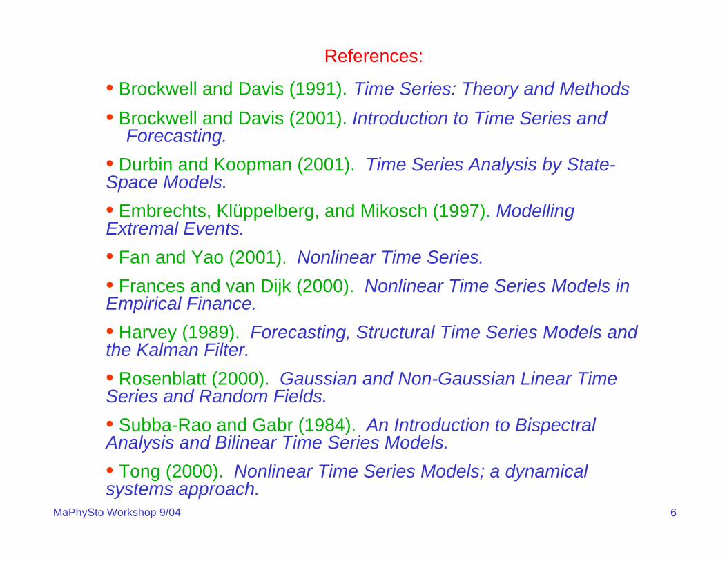
References:

• Brockwell and Davis (1991). Time Series: Theory and Methods• Brockwell and Davis (2001). Introduction to Time Series and

Forecasting.• Durbin and Koopman (2001). Time Series Analysis by State-Space Models.• Embrechts, Klüppelberg, and Mikosch (1997). ModellingExtremal Events.• Fan and Yao (2001). Nonlinear Time Series.• Frances and van Dijk (2000). Nonlinear Time Series Models in Empirical Finance.• Harvey (1989). Forecasting, Structural Time Series Models and the Kalman Filter.• Rosenblatt (2000). Gaussian and Non-Gaussian Linear Time Series and Random Fields.• Subba-Rao and Gabr (1984). An Introduction to BispectralAnalysis and Bilinear Time Series Models.• Tong (2000). Nonlinear Time Series Models; a dynamical systems approach.


Why nonlinear time series models?

≡What are the limitations of linear time series models?

≡What key features in data cannot be captured by linear time series models?

What diagnostic tools (visual or statistical) suggest incompatibility of a linear model with the data?

1. Introduction


Example: Z1, . . . , Zn ~ IID(0,σ2)

Sample autocorrelation function (ACF):

)0(ˆ)(ˆ

)(ˆγγ

=ρhhZ where ))(()(ˆ ||

||

1

1 ZZZZnh ht

hn

tt −−=γ +

−

=

− ∑

is the sample autocovariance function (ACVF).

-2.

-1.

0.

1.

2.

0 40 80 120 160 200

Series


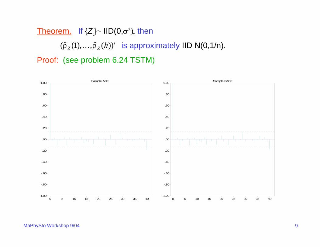
Theorem. If {Zt}~ IID(0,σ2), then

is approximately IID N(0,1/n).

Proof: (see problem 6.24 TSTM)

))'(ˆ,),1(ˆ( hZZ ρρ K

-1.00

-.80

-.60

-.40

-.20

.00

.20

.40

.60

.80

1.00

0 5 10 15 20 25 30 35 40

Sample ACF

-1.00

-.80

-.60

-.40

-.20

.00

.20

.40

.60

.80

1.00

0 5 10 15 20 25 30 35 40

Sample PACF


Cor. If {Zt}~ IID(0,σ2) and E|Z1|4 < ∞, then

is approximately IID N(0,1/n).))'(ˆ,),1(ˆ( 22 hZZ

ρρ K

-1.00

-.80

-.60

-.40

-.20

.00

.20

.40

.60

.80

1.00

0 5 10 15 20 25 30 35 40

Residual ACF: Abs values

-1.00

-.80

-.60

-.40

-.20

.00

.20

.40

.60

.80

1.00

0 5 10 15 20 25 30 35 40

Residual ACF: Squares


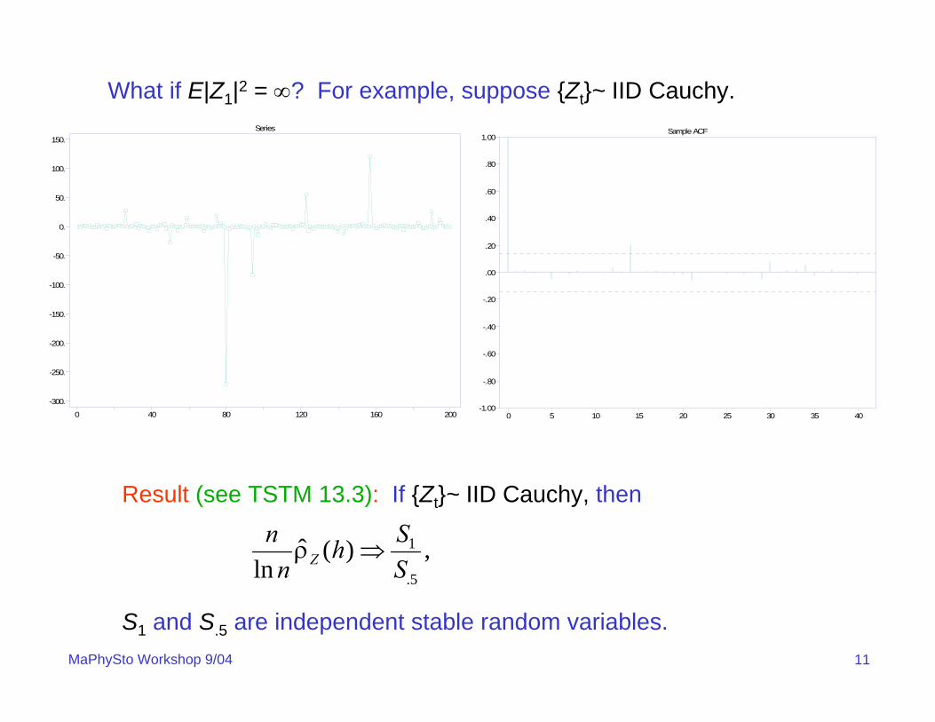
What if E|Z1|2 = ∞? For example, suppose {Zt}~ IID Cauchy.

-300.

-250.

-200.

-150.

-100.

-50.

0.

50.

100.

150.

0 40 80 120 160 200

Series

-1.00

-.80

-.60

-.40

-.20

.00

.20

.40

.60

.80

1.00

0 5 10 15 20 25 30 35 40

Sample ACF

Result (see TSTM 13.3): If {Zt}~ IID Cauchy, then

S1 and S.5 are independent stable random variables.

,)(ˆln 5.

1

SSh

nn

Z ⇒ρ ,)(ˆln 5.

1

SSh

nn

Z ⇒ρ


-1.00

-.80

-.60

-.40

-.20

.00

.20

.40

.60

.80

1.00

0 5 10 15 20 25 30 35 40


-1.00

-.80

-.60

-.40

-.20

.00

.20

.40

.60

.80

1.00

0 5 10 15 20 25 30 35 40


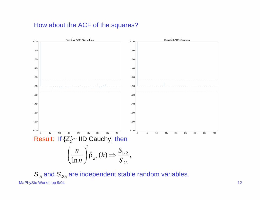
Result: If {Zt}~ IID Cauchy, then

S.5 and S.25 are independent stable random variables.

How about the ACF of the squares?

,)(ˆln 25.

2/12

2 SSh

nn

Z⇒ρ⎟

⎠⎞

⎜⎝⎛


Result: IID sequences {Zt} are time-reversible.

Application: If plot of time series does not look time- reversible, then it cannot be modeled as an IID sequence. Use the “flip and compare” inspection test!

Reversibility. The stationary sequence of random variables {Xt} is time-reversible if (X1, . . . ,Xn) =d (Xn, . . . ,X1).

-2.

-1.

0.

1.

2.

0 40 80 120 160 200

Series

-2.

-1.

0.

1.

2.

0 40 80 120 160 200

Series

14MaPhySto Workshop 9/04 -1.00

-.80

-.60

-.40

-.20

.00

.20

.40

.60

.80

1.00

0 5 10 15 20 25 30 35 40


-1.00

-.80

-.60

-.40

-.20

.00

.20

.40

.60

.80

1.00

0 5 10 15 20 25 30 35 40


Reversibility. Does the following series look time-reversible?

-30.

-20.

-10.

0.

10.

20.

0 40 80 120 160 200

Series

-1.00

-.80

-.60

-.40

-.20

.00

.20

.40

.60

.80

1.00

0 5 10 15 20 25 30 35 40

Sample ACF


1962 1967 1972 1977 1982 1987 1992 1997

020

4060

8010

012

014

0

time

clos

ing

pric

eClosing Price for IBM 1/2/62-11/3/00

2. Examples

16MaPhySto Workshop 9/041962 1967 1972 1977 1982 1987 1992 1997

time

-20

-10

010

100*

log(

retu

rns)

Log returns for IBM 1/3/62-11/3/00 (blue=1961-1981)


0 10 20 30 40

Lag

0.0

0.2

0.4

0.6

0.8

1.0

AC

F(a) ACF of IBM (1st half)

0 10 20 30 40

Lag

0.0

0.2

0.4

0.6

0.8

1.0

AC

F

(b) ACF of IBM (2nd half)

Sample ACF IBM (a) 1962-1981, (b) 1982-2000

Remark: Both halves look like white noise?


Lag

AC

F

0 10 20 30 40

0.0

0.2

0.4

0.6

0.8

1.0

(a) ACF, Abs Values of IBM (1st half)

Lag

AC

F

0 10 20 30 40

0.0

0.2

0.4

0.6

0.8

1.0

(b) ACF, Abs Values of IBM (2nd half)

Sample ACF of abs values for IBM (a) 1961-1981, (b) 1982-2000

Remark: Series are not independent white noise?


0 10 20 30 40

Lag

0.0

0.2

0.4

0.6

0.8

1.0

AC

F

(a) ACF, Squares of IBM (1st half)

0 10 20 30 40

Lag

0.0

0.2

0.4

0.6

0.8

1.0

AC

F

(b) ACF, Squares of IBM (2nd half)

ACF of squares for IBM (a) 1961-1981, (b) 1982-2000

Remark: Series are not independent white noise? Try GARCH or a stochastic volatility model.


day

log

retu

rns

(exc

hang

e ra

tes)

0 200 400 600 800

-20

24

lag

AC

F

0 10 20 30 40

0.0

0.2

0.4

0.6

0.8

1.0

lag

AC

F of

squ

ares

0 10 20 30 40

0.0

0.2

0.4

0.6

0.8

1.0

lag

AC

F of

abs

val

ues

0 10 20 30 40

0.0

0.2

0.4

0.6

0.8

1.0

Example: Pound-Dollar Exchange Rates (Oct 1, 1981 – Jun 28, 1985; Koopman website)


Year 1990

••••••••••

•••••

•••••••••••••••••

•••••

•

••••••

••••••••••••

••••

•••••••••••

••••••••

•••••••••

•••

••

••••

••••••

•••••

••

•

•••••••••••••••••••••

••

•

•••••

•

••••

•••••••

••••

•

••••••••••••

•

••••••

•••••

•

•••

•

••••••

•••••••••

•

•••••••

•

•••••••••••••

••••••••••

••••••••••

••••••••••••

••••••

•••••

••••••••

••••••••••••

•••••••

•••••••••••

••••••••••••

•

•••••••••••••

•••••

••••••••••••

••••••••

••••••

••••

06

14Jan Feb Mar Apr May Jun Jul Aug Sep Oct Nov Dec

Year 1991

••••••

••••••••••••

•••••••••

••••••••

•••••

••

•••••

••••••

••••••

••••••

•••••••••

••

•••

••••••

•

•••••••

•

••••••

••••••••

••••••••••••••

•••••

•••••

•

•

•

•••

•••••••••

••••••••

••••••••

••••••••••••

•

•••••••

••••

••••••

•••••••••••

•••••

•••••••

•

••••••••••••

••••

••••••••••

•••••••••••••••••••••••••••

••••••••

•••••

•••••

••••••••••

•••••••

•••••••••••••

•••••

••••••••••

•••••••••••••

••••••••••

•••••••••

06

14

Jan Feb Mar Apr May Jun Jul Aug Sep Oct Nov Dec

Year 1992

•

•••••••••

••••••••••••••••••••

••••••••

•

••••••••••

••

•••••

••

••

••••••••••

••

•

••

•••••

•••••

••••••

•••••••

•••

••••

••••••••••

•••

•••••••••

•••••••••

••••••

••

•

••

•

•

••

•

•••••••

•

•••••••

••••

•

•••••

••••••

•••••••••

••••••••••••

••••••

•••••••••

••••

••••••••

•••

••••••••

••••••••

•••••••••••••

•••••

••••••

••••••••••

••••••••

•••••••

•••••••••

•••••••••

•

•••••••

•

••••••••

••••••••••••

••••••••

•••••

•••••••0

614


Year 1993

••••••••••••

••••••••

•••••

•••••

•••••••••••

•••

••••

••

••••

••••

•

•

•••••••

•

•••••••••••

••

•••••••••

••••

••

••

••••••••

•••••••••

••••••••

•••••••••••

•

•••••••••••

••••

••••••

••

••••••

••

•••••

•••••••••••

•••••••••

•••••••

••••

••••••••••••

•••••••

•••••

••••••••

••••••

•••••••

•••••

•••••••

•••••

•••••

•••••

•••••••••

•

••••••••••••••••••••

••••

••••

•••••••

•••••••••••••••••••••

••••

•••••••••

••••••••••••0

614


Example: Daily Asthma Presentations (1990:1993)

Remark: Usually marginal distribution of a linear process is continuous.


0 1000 2000 3000 4000 5000

1022

1024

1026

1028

distance (m)

bed

elev

atio

n

Muddy Creek: surveyed every 15.24 meters, total of 5456m; 358 measurements

Degree AICc

0 1455

1 294.3

2 251.3

3 47.1

4 34.0

5 35.5

4 34.0

Muddy Creek- tributary to Sun River in Central Montana


0 1000 2000 3000 4000 5000distance (m)

-0.5

0.0

0.5

resi

dual

s de

g =

4

0 100 200 300 400lag (m)

0.0

0.2

0.4

0.6

0.8

1.0

acf

0 100 200 300 400lag (m)

0.0

0.2

0.4

0.6

0.8

1.0

acf

Blue = sampleRed = model


Minimum AICc ARMA model: ARMA(1,1) Yt = .574 Yt-1 + εt – .311 εt-1, {εt}~WN(0,.0564)

Some theory:

• LS estimates of trend parameters are asymptotically efficient.

• LS estimates are asymptotically indepof cov parameter estimates.

Noncausal ARMA(1,1) model: Yt = 1.743 Yt-1 + εt – .311 εt-1

Muddy Creek: residuals from poly(d=4) fit


Summary of models fitted to Muddy Creek bed elevation:

Degree AICc

0 1455

1 294.3

2 251.3

3 47.1

4 34.0

5 35.5

ARMA AICc

(1,2) 59.67

(2,1) 26.98

(2,1) 26.30

(1,1) 7.12

(1,1) 2.78

(1,1) 4.68

Muddy Creek (cont)


• About half of the CO2 emitted by humans accumulates in the atomosphere

• Other half is absorbed by “sink” processes on land andin the oceans

NEE= (Rh + Ra) – GPP (carbon flux)

GPP = Gross Primary Production (photosysynthesis)

Rh = Heterotrophic (microbial) respiration

Ra = autotrophic (plant) respiration.

The NEE data from the Harvard Forest consists of hourly measurements. We will aggregate over the day and consider dailydata from Jan 1, 1992 to Dec 31, 2001.

Go to ITSM Demo

Example: NEE=Net Ecosystem Exchange in Harvard Forest


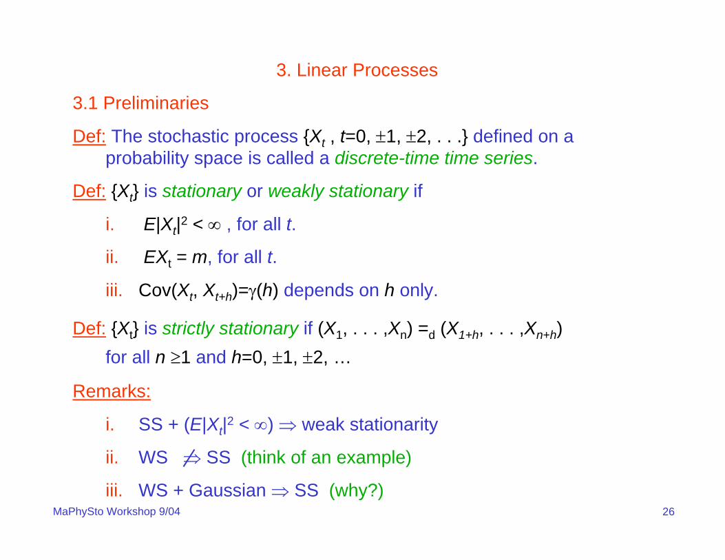
3.1 Preliminaries

Def: The stochastic process {Xt , t=0, ±1, ±2, . . .} defined on a probability space is called a discrete-time time series.

Def: {Xt} is stationary or weakly stationary if

i. E|Xt|2 < ∞ , for all t.

ii. EXt = m, for all t.

iii. Cov(Xt, Xt+h)=γ(h) depends on h only.

Def: {Xt} is strictly stationary if (X1, . . . ,Xn) =d (X1+h, . . . ,Xn+h) for all n ≥1 and h=0, ±1, ±2, …

Remarks:

i. SS + (E|Xt|2 < ∞) ⇒ weak stationarity

ii. WS ⇒ SS (think of an example)

iii. WS + Gaussian ⇒ SS (why?)

3. Linear Processes


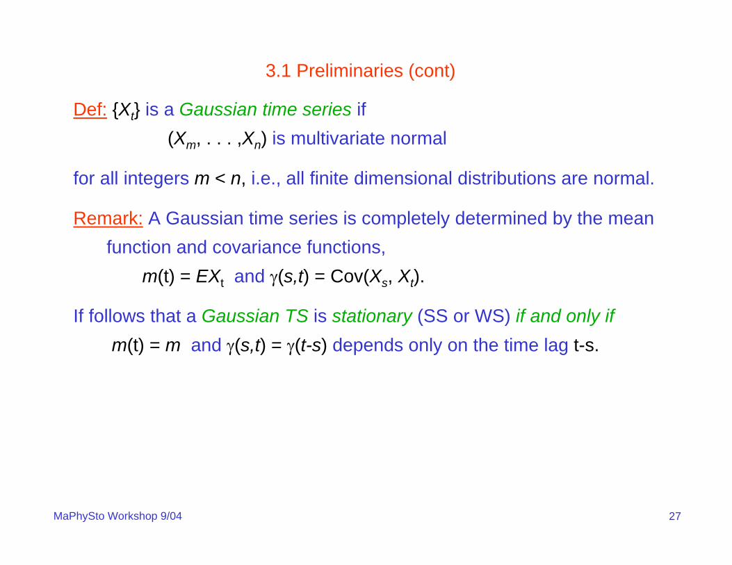
Def: {Xt} is a Gaussian time series if (Xm, . . . ,Xn) is multivariate normal

for all integers m < n, i.e., all finite dimensional distributions are normal.

Remark: A Gaussian time series is completely determined by the mean function and covariance functions,

m(t) = EXt and γ(s,t) = Cov(Xs, Xt).

If follows that a Gaussian TS is stationary (SS or WS) if and only ifm(t) = m and γ(s,t) = γ(t-s) depends only on the time lag t-s.

3.1 Preliminaries (cont)


Def: {Xt} is a linear time series with mean 0 if

where {Zt} ~ WN(0,σ2) and

Important remark: As a reminder WN means uncorrelated random

variables and not necessarily independent noise nor independent

Gaussian noise.

Proposition: A linear TS is stationary with

i. EXt = 0, for all t.

ii. and

If {Zt} ~ IID(0,σ2), then the linear TS is strictly stationary.

∑∞

−∞=−ψ=

jjtjt ZX ,

∑∞

−∞=+ψψσ=γ

jhjjh 2)( ∑∑

∞

−∞=

∞

−∞=+ ψψψ=ρ

jj

jhjjh 2/)(

.2 ∞<ψ∑∞

−∞=jj

3.1 Preliminaries (cont)


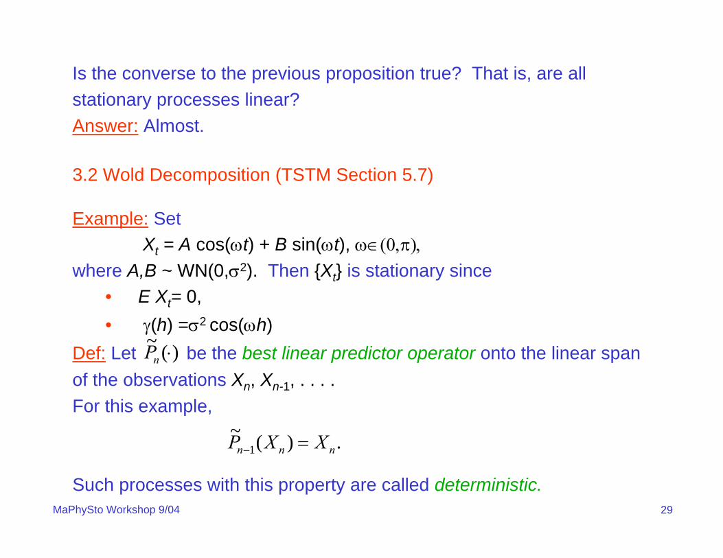
Is the converse to the previous proposition true? That is, are allstationary processes linear?Answer: Almost.

3.2 Wold Decomposition (TSTM Section 5.7)

Example: SetXt = A cos(ωt) + B sin(ωt), ω∈(0,π),

where A,B ~ WN(0,σ2). Then {Xt} is stationary since• E Xt= 0,• γ(h) =σ2 cos(ωh)

Def: Let be the best linear predictor operator onto the linear spanof the observations Xn, Xn-1, . . . .For this example,

Such processes with this property are called deterministic.

)(~ ⋅nP

.)(~1 nnn XXP =−


The Wold Decomposition. If {Xt} is a nondeterministic stationary time series with mean zero, then

wherei. ψ0 = 1, Σ ψj

2 <∞.

ii. {Zt} ~ WN(0,σ2)

iii. cov(Zs,Vt) = 0 for all s and t

iv. for all t.

v. for all s and t.

vi. {Vt} is deterministic.

The sequences {Zt}, {Vt}, and {ψt} are unique and can be written as

,0

∑∞

=− +ψ=

jtjtjt VZX

ttt ZZP =)(~

tts VVP =)(~

. ),(/)( ),(~0

21 ∑

∞

=−−− ψ−==ψ−=

jjtjtttjttjtttt ZXVZEZXEXPXZ

3.2 Wold Decomposition (cont)


Remark. For many time series (in particular for all ARMA processes) thedeterministic component Vt is 0 for all t and the series is then said to bepurely nondeterministic.

Example. Let Xt = Ut + Y, where {Ut} ~ WN(0,σ2) and is independent of

Y~(0,τ2). Then, in this case, Zt = Ut and Vt = Y (see TSTM, problem5.24).

Remarks:• If {Xt} is purely nondeterministic, then {Xt} is a linear process. • Spectral distribution for nondeterministic processes has the form

FX = FU + FV, where which has spectral density∑∞

=−ψ=

0jjtjt ZU

∑∞

=

λλ ψπ

σ=ψ

πσ

=λ0

22

22

|)(|2

||2

)(j

iijj eef



• If thenFX = FU + FV,

is the Lebesque decomposition of the spectral distribution function; FU is the absolutely continuous part and FV is the singular part.

Example. Let Xt = Ut + Y, where {Ut} ~ WN(0,σ2) and is independent of

Y~(0,τ2). Then)()(

2)( 0

22

λδτ+λπ

σ=λ dddFX

,0))(~( 21

2 >−=σ − ttt XPXE

Kolmogorov’s Formula.

.))(~( where,})(ln)2exp{(2 21

212ttt XPXEdf −

π

π−

− −=σλλππ=σ ∫

Clearly ∫π

π−

−∞>λλ>σ .)(ln iff 02 df



Example (TSTM problem 5.23).

This process has a spectral density function but is deterministic!!

.sin1 ),,0(~} , 2⎟⎟⎠

⎞⎜⎜⎝

⎛⎟⎠⎞

⎜⎝⎛

π=ψτψ= ∑

∞

−∞=− j

jWN{ZZX jtj

jtjt

Example (see TSTM problem 5.20). Let

and set

It follows that and is the WD for {Xt}.a) If {εt}~IID N(0,σ2), is {Zt} IID? Answer?b) If {εt}~IID(0,σ2), is {Zt} IID? Answer?

),,0(~}{ ,2 21 τεε−ε= − WNX tttt

5.3

)(5.)2(5.25.

)5.1(

1

322

2110

1

∑

∑∞

=−

−−−−−

∞

=−

−

ε−ε=

+ε−ε+ε−ε+ε−ε==

−=

jjt

jt

tttttj

tjtj

tt

X

XBZ

L

),0(~}{ 2σWNZt 15. −−= ttt ZZX



Remark: In this last example, the process {Zt} is called an allpassmodel of order 1. More on this type of process later.

Recall that the stationary time series {Xt} is time-reversible if (X1, . . . ,Xn) =d (Xn, . . . ,X1) for all n.

Go to ITSM Demo


3.3 Reversibility


The stationary time series {Xt} is time-reversible if (X1, . . . ,Xn) =d (Xn, . . . ,X1) for all n.

Theorem (Breidt & Davis 1991). Consider the linear time series {Xt}

where ψ(z) ≠ ±zr ψ(z-1) for any integer r. Assume either

(a) Z0 has mean 0 and finite variance and {Xt} has a spectral density positive almost everywhere.

or(b) 1/ψ(z)=π(z)=Σjπjzj, the series converging absolutely in some annulus

D containing the unit circle andπ(B)Xt = ΣjπjXt-j = Zt.

Then {Xt} is time-reversible if and only if Z0 is Gaussian.

,~}{ , IIDZZX tj

jtjt ∑∞

−∞=−ψ=

3.3 Reversibility


Remark: The condition ψ(z) ≠ ±zr ψ(z-1) on the filter precludes the filterfrom being symmetric about one of the coefficients. In this case, the time series would be time-reversible for non-Gaussian noise. Forexample, consider the series

Here ψ(z)=1 - .5z + z2 = z2 (1 - .5 z-1 + z2)= z2 ψ(z-1) and the series istime-reversible.

Proof of Theorem: Clearly any stationary Gaussian time series is time-reversible (why?). So suppose Z0 is nonGaussian and assume (a). If{Xt} time-reversible, then

~}{ ,5. 21 IIDZZZZX ttttt −− +−=

.)(

)()(

1)(

111 ∑

∞

−∞=−−− =

ψψ

=ψ

=ψ

=j

jtjttdtt ZaZBBX

BX

BZ

3.3 Reversibility (cont)


The first equality takes a bit of argument and relies on the spectralrepresentation of {Xt} given by

where Z(λ) is a process of orthogonal increments (see TSTM, Chapter 4).It follows, by the assumptions on the spectral density of {Xt} that

is well defined. So

and, by the assumption on ψ(z), the rhs is a non-trivial sum. Note that

),(],(

λ= ∫ππ−

λdZeX itt

),()(

1)(

1

],(

λψ

=ψ ∫

ππ−

λλ± dZe

eX

Bit

it m

.)(

)(1 ∑

∞

−∞=−− =

ψψ

=j

jtjtdt ZaZBBZ

12∑∞

−∞=

=j

ja Why? The above relation is a characterization of a Gaussian distribution(see Kagan, Linnik, and Rao (1973).)



Example: Recall for the example

and non-normal, the Wold decomposition is given by

where

By previous result, {Zt} cannot be time-reversible and hence is not IID.

),,0(~}{ ,2 21 τεε−ε= − IIDX tttt

,5. 1−−= ttt ZZX

.5.31

∑∞

=−ε−ε=

jjt

jttZ

Remark: This theorem can be used to show identifiability of theparameters and noise sequence for an ARMA process.



Motivating example: The invertible MA(1) process

has a non-invertible MA(1) representation,

Question: Can the {εt} also be IID?

Answer: Only if the Zt are Gaussian.

If the Zt are Gaussian, then there is an identifiability problem,

give the same model.

,1|| ),,0(~}{ , 21 <θσθ+= − IIDZZZX tttt

.1|| ),,0(~}{ , 221

1 <θσθεεθ+ε= −− WNX tttt

,1|| ),,(),( 2212 <θσθθ↔σθ −

3.4 Identifiability


For ARMA processes {Xt} satisfying the recursions,

casuality and invertibility are typically assumed, i.e.,

By flipping roots of the AR and MA polynomials from outside the unit circleto inside the unit circle, there are approximately 2p+q equivalentARMA representations of Xt driven with noise that is white (not IID). Foreach of these equivalent representations, the noise is only IID in theGaussian case.

Bottom line: For nonGaussian ARMA, there is a distinction betweencausal and noncausal; and invertible and non-invertible models.

tt

tqtqttptptt

ZBXBIIDZZZZXXX

)()(),,0(~}{ , 2

1111

θ=φ

σθ+θ+=φ−−φ− −−−− LL

1. |z|for 0)( and 0)( ≤≠θ≠φ zz

3.4 Identifiability (cont)


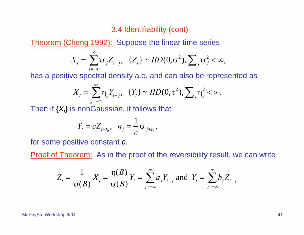
Theorem (Cheng 1992): Suppose the linear time series

has a positive spectral density a.e. and can also be represented as

Then if {Xt} is nonGaussian, it follows that

for some positive constant c.

, ),,0(~}{ , 22 ∞<ψσψ= ∑∑∞

−∞=− j jt

jjtjt IIDZZX

. ),,0(~}{ , 22 ∞<ητη= ∑∑∞

−∞=− j jt

jjtjt IIDYYX

,1 ,00 tjjttt c

ηcZY +− ψ==

Proof of Theorem: As in the proof of the reversibility result, we can write

and )()(

)(1 ∑∑

∞

−∞=−

∞

−∞=− ==

ψη

=ψ

=j

jtjtj

jtjttt ZbYYaYBBX

BZ



Now let {Y(s,t)} ~IID, Y(s,t) =d Y1 and set

Clearly, {Ut} is IID with same distribution as Z1. Consequently,

Since

Which by applying Theorems 5.6.1 and 3.3.1 in Kagan, Linnik, and Rao(1973), the sum above is trivial, i.e., there exists integers m and n suchthat am and bn are the only two nonzero coefficients. It follows that

∑∞

∞=

=-s

st tsYaU ).,(

.),( 1 ∑ ∑∑∞

−∞=

∞

−∞=

∞

−∞=

==t

ss

ttt

td tsYabUbY

,122 =∑ ∑∞

−∞=

∞

−∞=ts

st ab

.1 , njn

jntnt bηZbY +− ψ==



Cumulants and Polyspectra. We cannot base tests for linearity onsecond moments. A direct approach is to consider moments of higherorder and corresponding generalizations of spectral analysis.

Suppose that {Xt} satisfies supt E|Xt|k < ∞ for some k ≥ 3 and

for all t0,t1, . . . , tj, h=0, and j =0, . . ., k-1.

)()(1010 hththtttt jj

XXXEXXXE +++= LL

kth order cumulant. Coefficient, Ck(r1, . . . , rk-1), of ikz1z2…zk in the Taylor series expansion about (0,0,…,0) of

)exp(ln),,(11211 −++ +++=χ

krtkrttk XizXizXizEzz LK

3.5 Linear Tests


( )))()((),(3 µ−µ−µ−= ++ strtt XXXEsrC

3rd order cumulant.

If

then we define the bispectral density or (3rd – order polyspectral density)To be the Fourier transform,

-π ≤ ω1, ω2 ≤ π.

∞<∑ ∑ |),(| 3 srCr s

,),( )2(

1),( 21

s32213

ω−ω−∞

−∞=

∞

−∞=∑ ∑π

=ωω isir

r

esrCf

3.5 Linear Tests (cont)


kth - order polyspectral density.

Provided

-π ≤ ω1, . . . , ωk−1 ≤ π. (See Rosenblatt (1985) Stationary Sequences and Random Fields for more details.)

,|),,(|1 12

11 ∞<∑ ∑∑−

−r r kkr krrC KL

,),,( )2(

1

:),,(

1111

1 2 1

111

11

−−

−

ω−−ω−∞

−∞=

∞

−∞=

∞

−∞=−−

−

∑ ∑ ∑π

=ωω

kk

k

irir

r r rkkk

kk

errC

f

LKL

K



Applied to a linear process. If {Xt} has the Wold decomposition

with E|Zt|3 < ∞, EZt3 = η, and Σj |ψj| < ∞, then

where ψj := 0 for j < 0. Hence

),,0(~}{ , 2

0

σψ= ∑∞

=− IIDZZX t

jjtjt

sjrjj

jsrC ++

∞

−∞=

ψψψη= ∑),(3

).()()(4

),( 21212213

ω−ω−ω+ω ψψψπη

=ωω iiii eeef



The spectral density of {Xt} is

Hence, defining

we find that

Testing for constancy of φ(⋅) thus provides a test for linearity of {Xt} (seeSubba Rao and Gabr (1980)).

.|)(|2

)( 22

ωψπ

σ=ω ief

,)()()(

|),(|),(2121

2213

21 ω+ωωωωω

=ωωφfff

f

.2

),( 6

2

21 πση

=ωωφ



Gaussian linear process. If {Xt} is Gaussian, then EZ3=0, and the third

order cumulant is zero (why?). In fact Ck ≡ 0 for all k >2.

It follows that f3(ω1, ω2) ≡ 0 for all ω1, ω2 ∈[0,π]. A test for linear

Gaussianity can therefore be obtained by estimating f3(ω1,ω2) and

testing the hypothesis that f3 ≡ 0 (see Subba Rao and Gabr (1980)).



Suppose {Xt} is a purely nondeterministic process with WD given by

3.6 Prediction

).,0(~}{ , 2

0

σψ= ∑∞

=− WNZZX t

jjtjt

Then

so that

)(~1 tttt XPXZ −−=

. ~1

1 ∑∞

=−− ψ=

jjtjtt ZXP

Question. When does the best linear predictor equal the best predictor?

That is, when does

? ),| (~211 K−−− = ttttt XXXEXP


3.6 Prediction (cont)

? ),| (~211 K−−− = ttttt XXXEXP

Answer. Need

or, equivalently,),,(~

211 K−−− σ⊥−= tttttt XXXPXZ

.0),,|( 21 =−− Kttt XXZE

That is, BLP = BP

if and only if {Zt} is a Martingale-difference sequence.

Def. {Zt} is a Martingale-difference sequence wrt a filtration Ft (an

increasing sequence of sigma fields) if E|Zt| < ∞ for all t and

a) Zt is Ft measurableb) E(Zt | Ft-1)=0 a.s.


3.6 Prediction (cont)Remarks.1) An IID sequence with mean zero is a MG difference sequence.2) A purely nondeterministic Gaussian process is a Gaussian linear

process. This follows by the Wold decomposition and the fact that the resulting {Zt} sequence must be IID N(0,σ2) .

Example (Whittle): Consider the noncausal AR(1) process given byXt = 2 Xt-1 + Zt ,

where {Zt}~IID P(Zt = -1) = P(Zt = 0)=.5. Iterating backwards in time, wefind that

).5.5.(5.

5.5.5.

5.5.

22

1

12

12

1

L

M

−−−−=

−−=

−=

++

++

−

ttt

ttt

ttt

ZZZ

ZZX

ZXX


3.6 Prediction (cont)

is a binary expansion of a uniform (0,1) random variable. Notice thatfrom Xt, we can find Xt+1, by lopping off the first term in the binaryexpansion. This operation is exactly,

Xt+1 = 2 Xt mod 12Xt , if Xt < .5,2Xt -1, if Xt > .5.

1*

13

*3

2

*2

*1

32

21

,222

)5.5.(5.

+++++

+++

−=+++=

−−−−=

ttttt

tttt

ZZZZZ

ZZZX

L

L

⎩⎨⎧

=

Properties:


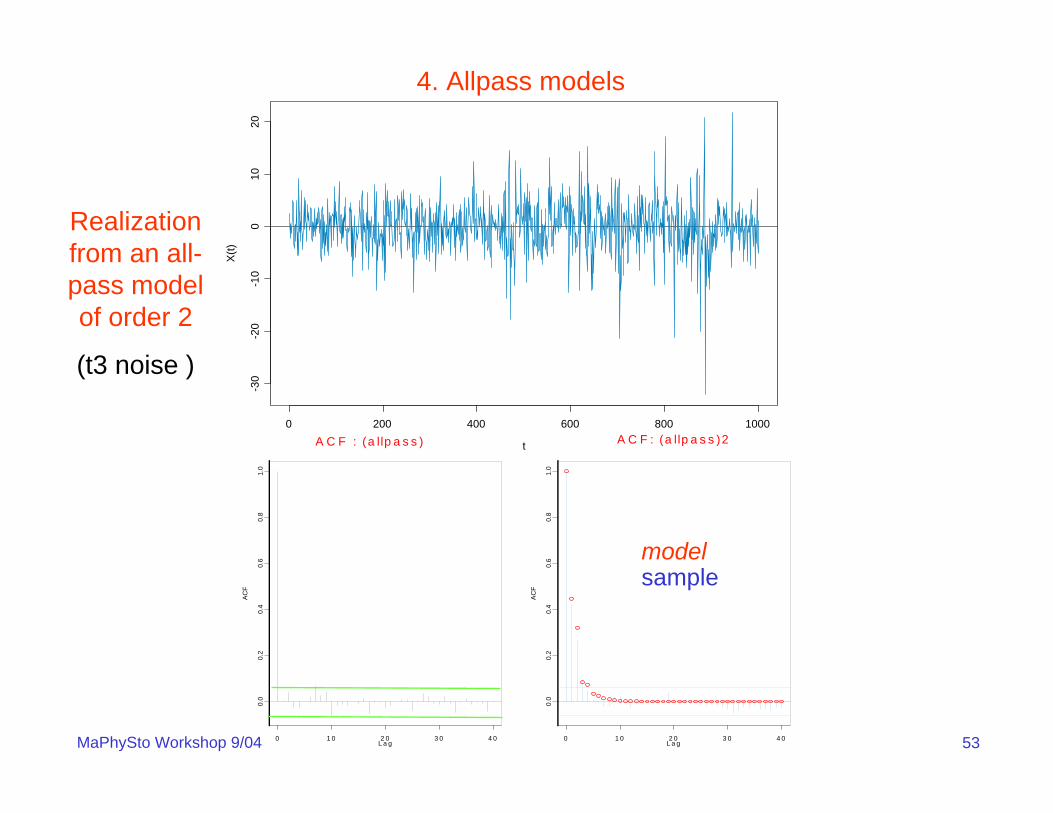
Realization from an all-pass model of order 2

(t3 noise )

0 1 0 2 0 3 0 4 0

0.0

0.2

0.4

0.6

0.8

1.0

L a g

AC

F

A C F : (a llp a s s )2

0 1 0 2 0 3 0 4 0

0.0

0.2

0.4

0.6

0.8

1.0

L a g

AC

F

A C F : (a llp a s s )

modelsample

t

X(t)

0 200 400 600 800 1000

-30

-20

-10

010

20

4. Allpass models


Causal AR polynomial: φ(z)=1−φ1z − − φpzp , φ(z) ≠ 0 for |z|≤1.

Define MA polynomial:

θ(z) = −zp φ(z−1)/φp = −(zp −φ1zp-1 − − φp)/ φp

≠ 0 for |z|≥1 (MA polynomial is non-invertible).

Model for data {Xt} : φ(B)Xt = θ(B) Zt , {Zt} ~ IID (non-Gaussian)

BkXt = Xt-k

Examples:

All-pass(1): Xt − φ Xt-1 = Zt − φ−1 Zt-1 , | φ | < 1.

All-pass(2): Xt − φ1 Xt-1 − φ2 Xt-2 = Zt + φ1/ φ2 Zt-1 − 1/ φ2 Zt-2

L

L

4. Allpass models (cont)


Properties:

• causal, non-invertible ARMA with MA representation

• uncorrelated (flat spectrum)

• zero mean

• data are dependent if noise is non-Gaussian

(e.g. Breidt & Davis 1991).

• squares and absolute values are correlated.

• Xt is heavy-tailed if noise is heavy-tailed.

πφσ

=π

σ

φφ

φ=ω

ω−

ωω−

22)(

)()( 2

22

22

22

pi

p

iip

Xe

eef

jt0j

jtp

1

t )()(

−

∞

=

−

∑ψ=φφ−

φ= ZZ

BBBX

p


Second-order moment techniques do not work

• least squares

• Gaussian likelihood

Higher-order cumulant methods

• Giannakis and Swami (1990)

• Chi and Kung (1995)

Non-Gaussian likelihood methods

• likelihood approximation assuming known density

• quasi-likelihood

Other

• LAD- least absolute deviation

• R-estimation (minimum dispersion)

Estimation for All-Pass Models


Noninvertible MA models with heavy tailed noise

Xt = Zt + θ1 Zt-1 + + θq Zt-q ,

a. {Zt} ~ IID nonnormal

b. θ(z) = 1 + θ1 z + + θq zq

No zeros inside the unit circle ⇒ invertible

Some zero(s) inside the unit circle ⇒ noninvertible

. . .

. . .

4.1 Application of Allpass models


Realizations of an invertible and noninvertible MA(2) processesModel: Xt = θ∗(B) Zt , {Zt} ~ IID(α = 1), whereθi(B) = (1 +1/2B)(1 + 1/3B) and θni(B) = (1 + 2B)(1 + 3B)

0 10 20 30 40

-40

-20

020

0 10 20 30 40

-300

-100

010

0

Lag

0 2 4 6 8 10

-0.2

0.2

0.6

1.0

ACF

Lag

0 2 4 6 8 10

-0.2

0.2

0.6

1.0

ACF


Application of all-pass to noninvertible MA model fitting

Suppose {Xt} follows the noninvertible MA model

Xt= θi(B) θni(B) Zt , {Zt} ~ IID.

Step 1: Let {Ut} be the residuals obtained by fitting a purely invertible MA model, i.e.,

So

Step 2: Fit a purely causal AP model to {Ut}

Z(B)~(B)U

). of version invertible theis ~( ,(B)U~(B)

(B)UˆX

tni

nit

ninitnii

tt

θθ

≈

θθθθ≈

θ=

.(B)Z(B)U~tnitni θ=θ


t

X(t)

0 200 400 600

2*10

56*

105

106

Volumes of Microsoft (MSFT) stock traded over 755 transaction days (6/3/96 to 5/28/99)


Analysis of MSFT:

Step 1: Log(volume) follows MA(4).

Xt =(1+.513B+.277B2+.270B3+.202B4) Ut (invertible MA(4))

Step 2: All-pass model of order 4 fitted to {Ut} using MLE (t-dist):

(Model using R-estimation is nearly the same.)

Conclude that {Xt} follows a noninvertible MA(4) which after refitting has

the form:

Xt =(1+1.34B+1.374B2+2.54B3+4.96B4) Zt , {Zt}~IID t(6.3)

6.26)ˆ( .)ZB960.43.116B1.135BB649.1(

)U02B2..131BB229..628B1(

t432

t432

=ν−++−=

−+−+−


Lag

AC

F

0 10 20 30 40

0.0

0.4

0.8

(a) ACF of Squares of Ut

Lag

AC

F

0 10 20 30 40

0.0

0.4

0.8

(b) ACF of Absolute Values of Ut

Lag

AC

F

0 10 20 30 40

0.0

0.4

0.8

(c) ACF of Squares of Zt

Lag

AC

F

0 10 20 30 40

0.0

0.4

0.8

(d) ACF of Absolute Values of Zt


Summary: Microsoft Trading Volume

Two-step fit of noninvertible MA(4):

• invertible MA(4): residuals not iid

• causal AP(4); residuals iid

Direct fit of purely noninvertible MA(4):

(1+1.34B+1.374B2+2.54B3+4.96B4)

For MCHP, invertible MA(4) fits.


0 1000 2000 3000 4000 5000distance (m)

-0.5

0.0

0.5

resi

dual

s de

g =

4

0 100 200 300 400lag (m)

0.0

0.2

0.4

0.6

0.8

1.0

acf

0 100 200 300 400lag (m)

0.0

0.2

0.4

0.6

0.8

1.0

acf



Minimum AICc ARMA model: ARMA(1,1)Yt = .574 Yt-1 + εt – .311 εt-1, {εt}~WN(0,.0564)

Muddy Creek: residuals from poly(d=4) fit


Causal ARMA(1,1) modelYt = .574 Yt-1

+ εt – .311 εt-1, {εt}~WN(0,.0564)

Noncausal ARMA(1,1) model: Yt = 1.743 Yt-1

+ εt – .311 εt-1

-1.00

-.80

-.60

-.40

-.20

.00

.20

.40

.60

.80

1.00

0 5 10 15 20 25 30 35 40


-1.00

-.80

-.60

-.40

-.20

.00

.20

.40

.60

.80

1.00

0 5 10 15 20 25 30 35 40


-1.00

-.80

-.60

-.40

-.20

.00

.20

.40

.60

.80

1.00

0 5 10 15 20 25 30 35 40


-1.00

-.80

-.60

-.40

-.20

.00

.20

.40

.60

.80

1.00

0 5 10 15 20 25 30 35 40



Example: Seismogram Deconvolution

Simulated water gun seismogram

• {βk} = wavelet sequence (Lii and Rosenblatt, 1988)

• {Zt} IID reflectivity sequence

0 200 400 600 800 1000

time

-500

0000

050

0000

0


Water Gun Seismogram Fit

Step 1: AICC suggests ARMA (12,13) fit

fit invertible ARMA(12,13) via Gaussian MLE

residuals not IID

Step 2: fit all-pass to residuals

order selected is r = 2.

residuals appear IID

Step 3: Conclude that {Xt} follows a non-invertible ARMA


0 5 10 15 20 25 30

lag (h)

0.0

0.2

0.4

0.6

0.8

1.0

acf

ACF of Wt2

0 5 10 15 20 25 30

lag (h)

0.0

0.2

0.4

0.6

0.8

1.0

acf

ACF of Zt2


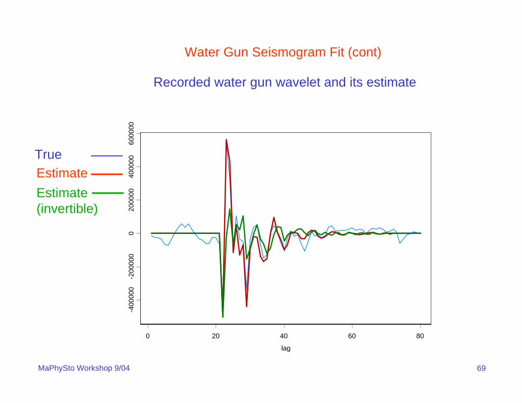
Water Gun Seismogram Fit (cont)

Recorded water gun wavelet and its estimate

0 20 40 60 80

-400

000

-200

000

020

0000

4000

0060

0000

lag

TrueEstimateEstimate(invertible)


Water Gun Seismogram Fit (cont)

Simulated reflectivity sequence and its estimates


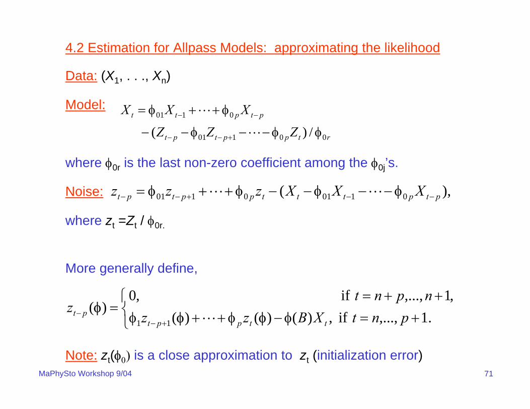
4.2 Estimation for Allpass Models: approximating the likelihood

Data: (X1, . . ., Xn)

Model:

where φ0r is the last non-zero coefficient among the φ0j’s.

Noise:

where zt =Zt / φ0r.

More generally define,

Note: zt(φ0) is a close approximation to zt (initialization error)

rtpptpt

ptptt

ZZZ

XXX

00101

0101

/)( φφ−−φ−−

φ++φ=

+−−

−−

L

L

),( 01010101 ptptttpptpt XXXzzz −−+−− φ−−φ−−φ++φ= LL

⎩⎨⎧

+=φ−φ++φ++=

=+−

− .1,..., if ,)()()(,1,..., if ,0

)(11 pntXBzz

npntz

ttpptpt φφ

φL


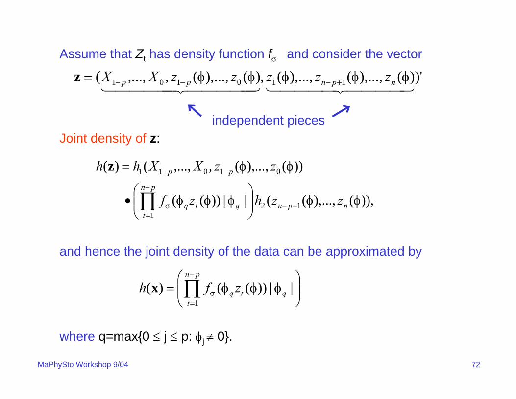
Assume that Zt has density function fσ and consider the vector

Joint density of z:

and hence the joint density of the data can be approximated by

where q=max{0 ≤ j ≤ p: φj ≠ 0}.

)')(),...,(),...,(,)(),...,(,,...,( 110101 4444 34444 2144444 344444 21φφφφφ npnpp zzzzzXX +−−−=z

independent pieces

)),(),...,(( ||))((

))(),...,(,,...,()(

121

01011

φφφ

φφ

npn

pn

tqtq

pp

zzhzf

zzXXhh

+−

−

=σ

−−

⎟⎟⎠

⎞⎜⎜⎝

⎛φφ•

=

∏

z

⎟⎟⎠

⎞⎜⎜⎝

⎛φφ= ∏

−

=σ

pn

tqtq zfh

1

||))(()( φx


Log-likelihood:

where fσ(z)= σ−1 f(z/σ).

Least absolute deviations: choose Laplace density

and log-likelihood becomes

Concentrated Laplacian likelihood

Maximizing l(φ) is equivalent to minimizing the absolute deviations

))((ln|)|/ln()(),(1

1 φφ ∑−

=

− φσ+φσ−−=σpn

ttqq zfpnL

|)|2exp(2

1)( zzf −=

||/ ,/|)(|2ln)(constant1

q

pn

ttzpn φσ=κκ−κ−− ∑

−

=

φ

|)(|ln)(constant)(1

φφ ∑−

=

−−=pn

ttzpnl

.|)(|)(1

n φφ ∑−

=

=pn

ttzm


Assumptions for MLE

Assume {Zt} iid fσ(z)=σ−1f(σ−1z) with

• σ a scale parameter

• mean 0, variance σ2

• further smoothness assumptions (integrability,symmetry, etc.) on f

• Fisher information:

Results

Let γ(h) = ACVF of AR model with AR poly φ0(.) and

dzzfzfI )(/))('(~ 22 ∫−σ=

p1kj,k)]-j([ =γ=Γp

))1~(2

1,0() ˆ( 1220MLE

−Γσ−σ

→− p

D

INn φφ


Further comments on MLE

Let α=(φ1, . . . , φp, σ /|φp|, β1, . . . , βq), where β1, . . . , βq are

the parameters of pdf f.

Set

(Fisher Information)

{ }

dzzfzfzf

dzzfzfzfz

dzzfzfz

dzzfzf

T

f

p

p

0

0

0

0

00

0

0

0

0

00

00

ββ

ββ

ββ

ββ

ββ

ββ

ββ

∂∂

∂∂

=

∂∂

α−=

−α=

σ=

∫

∫

∫∫

−+

−+

−

);();();(

1)(I

);();();('L

1);(/));('(K

);(/));('(I

11,0

2221,0

220


Under smoothness conditions on f wrt β1, . . . , βq we have

where

Note: is asymptotically independent of and

),,0() ˆ( 10MLE

−∑→− NnD

αα

⎥⎥⎥⎥⎥⎥

⎦

⎤

⎢⎢⎢⎢⎢⎢

⎣

⎡

−−−−−−

Γσ−σ

=∑−−−−−

−−−−−

−

−

11111

11111

1220

1

)'ˆ(ˆ)'ˆ()'ˆ('ˆ)'ˆ(

)1ˆ(21

LKLIKLLKLILKLILKLILK

I

ff

ff

p

00

00

ˆMLEφ ˆ MLE1,p+α ˆ

MLEβ


Asymptotic Covariance Matrix

• For LS estimators of AR(p):

• For LAD estimators of AR(p):

• For LAD estimators of AP(p):

• For MLE estimators of AP(p):

),0() ˆ( 120LS

−Γσ→− p

DNn φφ

))0(4

1,0() ˆ( 12220LAD

−Γσσ

→− p

D

fNn φφ

))1ˆ(2

1,0() ˆ( 1220MLE

−Γσ−σ

→− p

D

INn φφ

)|)|)0(2(2

|)(|Var,0() ˆ( 122

12

10LAD

−

σ

Γσ−σ

→− p

D

ZEfZNn φφ


Laplace: (LAD=MLE)

Students tν, ν >2:

LAD:

MLE:

Student’s t3:

LAD: .7337

MLE: 0.5

ARE: .7337/.5=1.4674

)1ˆ(21

21

|)|)0(2(2|)(|Var

221

21

−σ==

−σ σ IZEfZ

))2/)1(()2(4)2/()1(()2/)1((8

)2( 2222 +νΓ−ν−νΓ−νπ

+νΓ−ν

12)3)(2(

)1ˆ(21

2

+ν−ν=

−σ I


R-Estimation:

Minimize the objective function

where {z(t)(φ)} are the ordered {zt(φ)}, and the weight function ϕ

satisfies:

• ϕ is differentiable and nondecreasing on (0,1)

• ϕ´ is uniformly continuous

• ϕ(x) = −ϕ(1−x)

Remarks:

•

• For LAD, take

)(1

( )(1t

φφ) t

pn

zpntS ∑

−

=⎟⎟⎠

⎞⎜⎜⎝

⎛+−

ϕ=

)(1

((1t

φφ)

φ) t

pnt zpn

RS ∑−

=⎟⎟⎠

⎞⎜⎜⎝

⎛+−

ϕ=

1.x1/2 1,

1/2,x0 1,-)(

⎩⎨⎧

<<<<

=ϕ x


Assumptions for R-estimation

Assume {Zt} iid with density function f (distr F)

• mean 0, variance σ2

Assume weight function ϕ is nondecreasing and continuouslydifferentiable with ϕ(x) = −ϕ(1−x)

Results

Set

If then

∫∫∫ ϕ=ϕ=ϕ= −−1

0

11

0

11

0

2 )('))((L~ ,)()(K~ ,)(J~ dsssFfdsssFdss

))~~(2

~~,0() ˆ( 12

22

22

0R−Γσ

−σ−σ

→− p

D

KLKJNn φφ

,~~2 KL >σ


Further comments on R-estimation

ϕ(x) = x−1/2 is called the Wilcoxon weight function

By formally choosing

we obtain

That is R = LAD, asymptotically.

The R-estimation objective function is smoother than the

LAD-objective function and hence easier to minimize.

1.x1/2 1,

1/2,x0 1,-)(

⎩⎨⎧

<<<<

=ϕ x

.|)|)0(2(2

|)(|Var)~~(2

~~12

21

2112

22

22−

σ

− Γσ−σ

=Γσ−σ

−σpp ZEf

ZKLKJ

82MaPhySto Workshop 9/04phi

-0.5 0.0 0.5

22.0

22.5

23.0

23.5

24.0

24.5

Objective Functions

R-estimation

LAD


Summary of asymptotics

Maximum likelihood:

R-estimation

Least absolute deviations:

))1~(2

1,0() ˆ( 1220MLE

−Γσ−σ

→− p

D

INn φφ

)|)|)0(2(2

|)(|Var,0() ˆ( 122

12

10LAD

−

σ

Γσ−σ

→− p

D

ZEfZNn φφ

))~~(2

~~,0() ˆ( 12

22

22

0R−Γσ

−σ−σ

→− p

D

KLKJNn φφ


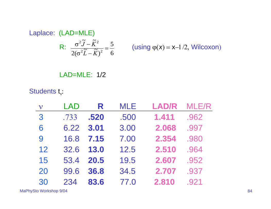
Laplace: (LAD=MLE)

R: (using ϕ(x) = x−1/2, Wilcoxon)

LAD=MLE: 1/2

Students tν:

65

)~~(2

~~22

22

=−σ

−σKLKJ

ν LAD R MLE LAD/R MLE/R3 .733 .520 .500 1.411 .9626 6.22 3.01 3.00 2.068 .9979 16.8 7.15 7.00 2.354 .98012 32.6 13.0 12.5 2.510 .96415 53.4 20.5 19.5 2.607 .95220 99.6 36.8 34.5 2.707 .93730 234 83.6 77.0 2.810 .921


Central Limit Theorem (R-estimation)

• Think of u = n1/2(φ−φ0) as an element of RRp

• Define

where Rt(φ) is the rank of zt(φ) among z1(φ), . . ., zn-p(φ).

• Then Sn(u) → S(u) in distribution on C(RRp), where

• Hence,

,)()1) ((- )()

1) (()(

10

0

1

1/2-0

-1/20 ∑∑

−

=

−

=⎟⎟⎠

⎞⎜⎜⎝

⎛+−

ϕ⎟⎟⎠

⎞⎜⎜⎝

⎛+

+−+

ϕ=pn

tt

tpn

tt

tn z

pnRnz

pnnRS φ

φφ

φ uuu

),||)~~(2 ,(~ ,'')~~(||)( 220

222210 prpr KJNKLS Γσφ−σ+Γσ−σφ= −−−− 0NNuuuu

)||)~~(2

~~,(~

)~~(2||

)(minarg)ˆ()(minarg

122

022

2212

20

02/1

−− Γσφ−σ

−σΓσ

−σφ

−=

→−=

pr

pr

D

Rn

KLKJN

KL

SnS

0N

uu φφ


Main ideas (R-estimation)

• Define

where Fz is the df of zt.

• Using a Taylor series, we have

• Also,

• Hence

,)())((- )())(()(~1

01

1/2-0 ∑∑

−

=

−

=

ϕ+ϕ=pn

tttz

pn

tttzn zzFnzzFS φφ uu

uuNu

uuuu

prD

pn

t

ttz

pn

t

ttzn

K

zzFnzzFnS

Γσφ−→

⎟⎟⎠

⎞⎜⎜⎝

⎛∂∂

∂ϕ+⎟⎟

⎠

⎞⎜⎜⎝

⎛∂

∂ϕ

−−

−

=

−−

=∑∑

210

1

02

1-1

1

01/2-

||~''

')())(('2 )())(('~)(~

φφφ

φφ

).1(||/~')(~)( 022

prpnn oLSS +φΓσσ=− − uuuu

).||)~~(2 ,(~ ,'')~~(||)( 220

222210 prprDn KJNKLS Γσφ−σ+Γσ−σφ→ −−−− 0NNuuuu


Order Selection:

Partial ACF From the previous result, if true model is of order r and fitted

model is of order p > r, then

where is the pth element of .

Procedure:

1. Fit high order (P-th order), obtain residuals and estimate scalar,

by empirical moments of residuals and density estimates.

)|)|)0(2(2

|)(|Var,0(ˆ2

12

1,

2/1

ZEfZNn LADp −σ

→φσ

LADp,φ LADφ

21

212

|)|)0(2(2|)(|VarZEf

Z−σ

=θσ


2. Fit AP models of order p=1,2, . . . , P via LAD and obtain p-th coefficient

for each.

3. Choose model order r as the smallest order beyond which the estimated

coefficients are statistically insignificant.

Note: Can replace with if using MLE. In this case

for p > r

pp,φ

pp,φ MLE,ˆpφ

).)1ˆ(2

1,0(ˆ2,

2/1

−σ→φ

INn MLEp


AIC: 2p or not 2p?

• An approximately unbiased estimate of the Kullback-Leiber index of fitted

to true model:

• Penalty term for Laplace case:

• Penalty term can be estimated from the data.

pZEf

ZEfZLpAIC X ⎟⎟

⎠

⎞⎜⎜⎝

⎛−

σ−σ

+κ−= σ

σ

1||)0(2

|)|)0(2(|)(|Var)ˆ,ˆ(2:)(

1

2

21

21φ

ppZEf

ZEfZ

=⎟⎟⎠

⎞⎜⎜⎝

⎛−

σ−σ

σ

σ

1||)0(2

|)|)0(2(|)(|Var

1

2

21

21


Sample realization of all-pass of order 2

t

X(t)

0 100 200 300 400 500

-40

-20

020

(a) Data From Allpass Model

Lag

AC

F

0 10 20 30 40

0.0

0.2

0.4

0.6

0.8

1.0

(b) ACF of Allpass Data

Lag

AC

F

0 10 20 30 40

0.0

0.2

0.4

0.6

0.8

1.0

(c) ACF of Squares

Lag

AC

F

0 10 20 30 40

0.0

0.2

0.4

0.6

0.8

1.0

(d) ACF of Absolute Values


Simulation results:

• 1000 replicates of all-pass models

• model order parameter value

1 φ1 =.5

2 φ1=.3, φ2=.4

• noise distribution is t with 3 d.f.

• sample sizes n=500, 5000

• estimation method is LAD


To guard against being trapped in local minima, we adopted the following strategy.

• 250 random starting values were chosen at random. For model of order p, k-th starting value was computed recursively as follows:

1. Draw iid uniform (-1,1).2. For j=2, …, p, compute

• Select top 10 based on minimum function evaluation.

• Run Hooke and Jeeves with each of the 10 starting values and choose best optimized value.

)()(22

)(11 ,...,, k

ppkk φφφ

⎥⎥⎥

⎦

⎤

⎢⎢⎢

⎣

⎡

φ

φφ−

⎥⎥⎥

⎦

⎤

⎢⎢⎢

⎣

⎡

φ

φ=

⎥⎥⎥

⎦

⎤

⎢⎢⎢

⎣

⎡

φ

φ

−

−−

−−

−

−)(

1,1

)(1,1

)(

)(1,1

)(1,1

)(1,

)(1

kj

kjj

kjj

kjj

kj

kjj

kj

MMM


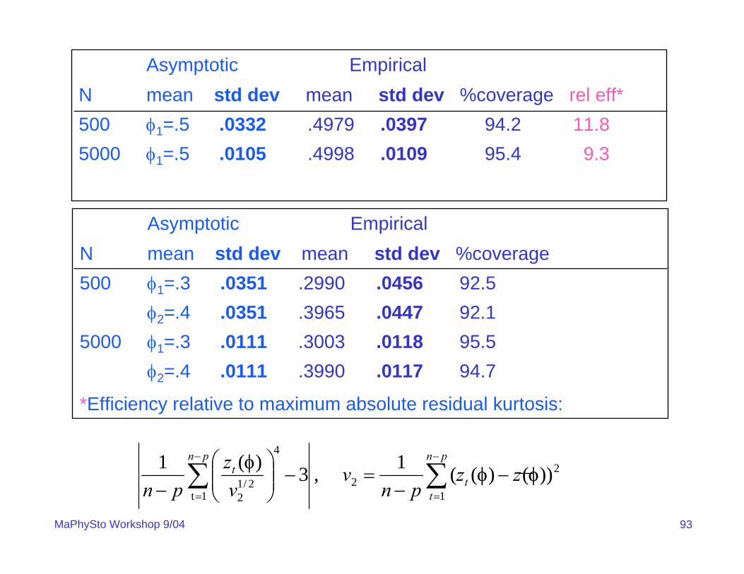
Asymptotic EmpiricalN mean std dev mean std dev %coverage rel eff*500 φ1=.5 .0332 .4979 .0397 94.2 11.85000 φ1=.5 .0105 .4998 .0109 95.4 9.3

Asymptotic EmpiricalN mean std dev mean std dev %coverage500 φ1=.3 .0351 .2990 .0456 92.5

φ2=.4 .0351 .3965 .0447 92.15000 φ1=.3 .0111 .3003 .0118 95.5

φ2=.4 .0111 .3990 .0117 94.7

*Efficiency relative to maximum absolute residual kurtosis:

2

12

1t

4

2/12

))()((1 , 3)(1φφ

φ zzpn

vvz

pn t

pn

t

pnt −

−=−⎟⎟

⎠

⎞⎜⎜⎝

⎛− ∑∑

−

=

−

=


Empirical Empirical LADN mean std dev mean std dev500 φ1=.5 .4978 .0315 .4979 .03975000 φ1=.5 .4997 .0094 .4998 .0109500 φ1=.3 .2988 .0374 .2990 .0456

φ2=.4 .3957 .0360 .3965 .04475000 φ1=.3 .3007 .0101 .3003 .0118

φ2=.4 .3993 .0104 .3990 .0117

R-Estimator: Minimize the objective fcn

where {z(t)(φ)} are the ordered {zt(φ)}.

)(21

1( )(

1tφφ) t

pn

zpntS ∑

−

=⎟⎟⎠

⎞⎜⎜⎝

⎛−

+−=

Nonlinear Time Series Modelingrdavis/lectures/Cop_P1.pdfNonlinear Time Series Modeling ... Time...

Documents

Transcript of Nonlinear Time Series Modelingrdavis/lectures/Cop_P1.pdfNonlinear Time Series Modeling ... Time...