Nonlinear time series analysis of jerk congenital...

J Comput Neurosci (2006) 21:153–170DOI 10.1007/s10827-006-7816-4

Nonlinear time series analysis of jerk congenital nystagmusO. E. Akman · D. S. Broomhead · R. A. Clement ·R. V. Abadi

Received: 14 July 2005 / Revised: 12 December 2005 / Accepted: 16 February 2006 / Published online: 26 May 2006C© Springer Science + Business Media, LLC 2006

Abstract Nonlinear dynamics provides a complementaryframework to control theory for the quantitative analysis ofthe oculomotor control system. This paper presents a num-ber of findings relating to the aetiology and mechanics ofthe pathological ocular oscillation jerk congenital nystag-mus (jerk CN). A range of time series analysis techniqueswere applied to recorded jerk CN waveforms, and also tosimulated jerk waveforms produced by an established modelin which the oscillations are a consequence of an unstableneural integrator. The results of the analysis were then inter-preted within the framework of a generalised model of theunforced oculomotor system.

Action Editor: Peter Latham

O. E. Akman (�)The School of Mathematics, The University of Manchester,P.O. Box 88, Manchester, M60 1QD UKPresent address: Mathematics Institute, University of Warwick,Coventry CV4 7AL UKe-mail: [email protected]

D. S. BroomheadThe School of Mathematics, The University of Manchester,P.O. Box 88, Manchester, M60 1QD UKe-mail: [email protected]

R. A. ClementVisual Sciences Unit, Institute of Child Health, U.C.L.,30 Guilford St., London, WC1N 1EH UKe-mail: [email protected]

R. V. AbadiFaculty of Life Sciences, Moffat Building,The University of Manchester, Sackville St., Manchester M601QD UKe-mail: [email protected]

This work suggests that for jerk oscillations, the origin ofthe instability lies in one of the five oculomotor subsystems,rather than in the final common pathway (the neural integra-tor and muscle plant). Additionally, experimental estimatesof the linearised foveation dynamics imply that a refixat-ing fast phase induced by a near-homoclinic trajectory willresult in periodic oscillations. Local dimension calculationsshow that the dimension of the experimental jerk CN data in-creases during the fast phase, indicating that the oscillationsare not periodic, and hence that the refixation mechanismis of greater complexity than a homoclinic reinjection. Thedimension increase is hypothesised to result either from asignal-dependent noise process in the saccadic system, orthe activation of additional oculomotor components at thebeginning of the fast phase. The modification of a recentsaccadic system model to incorporate biologically realisticsignal-dependent noise is suggested, in order to test the firstof these hypotheses.

Keywords Nonlinear dynamics . Oculomotor control .

Jerk CN . Neural integrator . Homoclinic reinjection .

Signal-dependent noise

1. Introduction

The oculomotor system is well suited to the quantitativestudy of sensorimotor processing (Robinson, 1986). Singlecell recordings have enabled the identification of many ofthe neural pathways associated with eye movement control,enabling meaningful mathematical models of the controlcircuitry to be developed. Additionally, eye movementscan be accurately recorded in the laboratory, providinghigh quality time series data which can be used to test anddevelop such models.

Springer

154 J Comput Neurosci (2006) 21:153–170

The majority of models developed thus far have beenbased on control theory (Carpenter, 1988). These modelshave had considerable success in elucidating the functionalorganisation of the oculomotor system (Leigh and Zee,1999). A significant achievement of the control approachhas been the prediction of a common neural integrator,subsequently confirmed experimentally (Robinson, 1968;Cohen and Komatsuzaki, 1972; Zee et al., 1981; Cannonand Robinson, 1987). This successful prediction supportedthe assumption that individual blocks of the control modelscan be directly identified with separate classes of neurons inthe brain stem. However, in subsequent modelling of patho-logical eye movements (Optican and Zee, 1984; Jacobs andDell’Osso, 2004), the number of assumed blocks far ex-ceeds the number of known classes of neurons so that thisassumption becomes questionable, motivating the need foralternative modelling strategies.

Techniques based on nonlinear dynamics provide a com-plementary approach to control theory in the analysis ofthe oculomotor system (Clement et al., 2002a). The lastfew years have seen the development of differential equa-tion models (Gancarz and Grossberg, 1998; Broomheadet al., 2000) together with the application of time seriesanalysis to eye movement recordings (Shelhamer, 1997;Abadi et al., 1997; Clement et al., 2002b, c). A previ-ous paper showed that one advantage of the nonlinear dy-namics approach is the capacity of bifurcation analysis toreveal the full range of behaviour that a model is capa-ble of producing (Akman et al., 2005). The present pa-per describes the use of nonlinear time series techniquesto investigate hypotheses suggested by oculomotor mod-els regarding the aetiology and mathematical characterisa-tion of oscillatory ocular disorders. It is demonstrated thatthese techniques provide a quantitative means of testingsuch models, and their implications, against experimentaldata.

Section 2 of the paper introduces the reader to the func-tional organisation of the different oculomotor subsystems.Thereafter, Section 3 details the construction of a generalisedmodel of the unforced oculomotor system for horizontal eyemovements. This model provides a framework for interpret-ing the results of the time series analysis. The characteri-sation of a pathological oculomotor system in terms of themodel is discussed in Section 4, where it is hypothesised thatthe condition known as jerk congenital nystagmus (jerk CN)is a consequence of a bifurcation. Section 5 describes thedata reconstruction method (delay embedding) which formsthe basis of the computational techniques used to check andexpand upon this hypothesis. The results of applying thesetechniques to both recorded jerk CN data and waveformssimulated by an unstable neural integrator model are pre-sented in Section 6. The implications of the work are dis-cussed in Section 7.

The results of this study indicate that in jerk CN, the ini-tial instability is caused by a fixed point (that corresponds tostable gaze at the primary position, 0◦) losing stability in a1-dimensional bifurcation. Moreover, estimates of the eigen-values of the linearisation at this fixed point suggest that themost likely source of this bifurcation is one of the oculomo-tor subsystems, rather than the neural integrator or muscleplant. In addition, a model of the linearised dynamics aboutthe fixed point derived from the eigenvalue estimates impliesthe simplest model of a refixating fast phase—a determin-istic reinjection induced by a near-homoclinic orbit—willresult in a limit cycle attractor. Local dimension calculationsshow that the dimension of the jerk CN attractor increasesduring the fast phase, implying that a limit cycle is not areasonable approximation to the true behaviour, from whichit follows that the fast phase is dynamically more complexthan a homoclinic reinjection. Two possible mechanisms thatcould account for the dimension increase are discussed: theactivation of additional oculomotor components as the cycleenters the fast phase, or a signal-dependent increase in thevariance of the saccadic control signal.

More generally, it is suggested that the eigenvalues oflinearisation and local dimension are quantitative experi-mental measurements that can be used in the developmentof comprehensive CN models. Within this framework, it isproposed that a model capable of simulating the local di-mension variation could be obtained by modifying an exist-ing saccadic system model to incorporate signal-dependentnoise.

2. Oculomotor control and congenital nystagmus

The oculomotor system controls the movement of the eyesso as to ensure that the image of the object of interest fallson the high resolution region of the retina called the fovea.This process is referred to as foveation (Ditchburn, 1973).Resolution of detail decreases sharply away from the fovea,and is also degraded if images slip over the fovea at veloc-ities greater than a few degrees per second. Optimal visualperformance is therefore only attained when images are heldsteady on this region (Westheimer and McKee, 1975).

Depending on the stimuli and viewing conditions, thefoveation task can involve up to five oculomotor subsys-tems: the saccadic, smooth pursuit, vestibular, optokineticand vergence systems. The saccadic system provides rapidshifts of gaze (saccades) to bring about foveation of newtargets. The smooth pursuit system matches eye velocitywith target velocity to provide a stable foveal image whentracking slow-moving objects in the visual field. The func-tion of the vestibular system is to stabilise gaze during briefhead rotations by generating an eye movement which has ve-locity equal and opposite to head velocity. The optokinetic

Springer

J Comput Neurosci (2006) 21:153–170 155

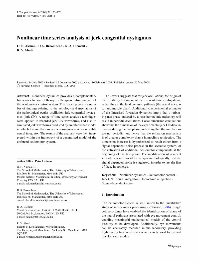
Fig. 1 Functional organisation of the oculomotor system for horizon-tal eye movements. The saccadic system is driven by target positionT while the smooth pursuit system responds to target velocity T . Thevestibular and optokinetic systems are driven by a head velocity sig-nal H provided by the semicircular canals and visual system respec-

tively. The vergence system is driven by the distance to the target D.bK = velocity signal from subsystem K, b = velocity signal from theOCS, n = position signal from the neural integrator, g = horizontal eyeposition. (Modified from Fig. 12.2 of Carpenter (1988))

system matches eye velocity to the global retinal image ve-locity in order to maintain stable gaze during sustained headmotion. Finally, the vergence system maintains foveationduring motion of the target towards or away from the eyes(Carpenter, 1988; Leigh and Zee, 1999).

The vestibular system is driven by non-visual signals fromthe semicircular canals, while the other systems are driven byvisual signals encoding target information. In response to thissensory input, each of the oculomotor subsystems generates avelocity-coded command signal. A copy of this signal is sentto a complex of neurons, the common neural integrator (NI),which integrates it to produce a position-coded signal. Theposition and velocity signals are then summed and relayed tothe relevant ocular motoneurons. These send the final motorcommand to the eye muscles, producing a shift in the eyeposition (Carpenter, 1988; Leigh and Zee, 1999). In controlmodels, the ocular motoneurons and eye muscles are referredto collectively as the muscle plant. Here, the five oculomotorsubsystems will be referred to as the oculomotor commandsystem (OCS). A schematic representation of the oculomotorsystem architecture is shown in Fig. 1.

Congenital nystagmus (CN) is an involuntary, bilateraloscillation of the eyes that is present in approximately 1in 4000 of the population (Abadi and Dickinson, 1986;Abadi and Bjerre, 2002). The oscillations are conjugateand occur primarily in the horizontal plane. The oscillationgenerally consists of a slow phase, which takes the retinalimage of the visual target away from the fovea, followed bya fast or slow phase which moves the image back onto thefovea (Dell’Osso and Daroff, 1975; Abadi and Dickisnon,1986; Abadi et al., 1991). CN subjects tend to have poorvisual acuity due to the reduced foveation time (Abadi and

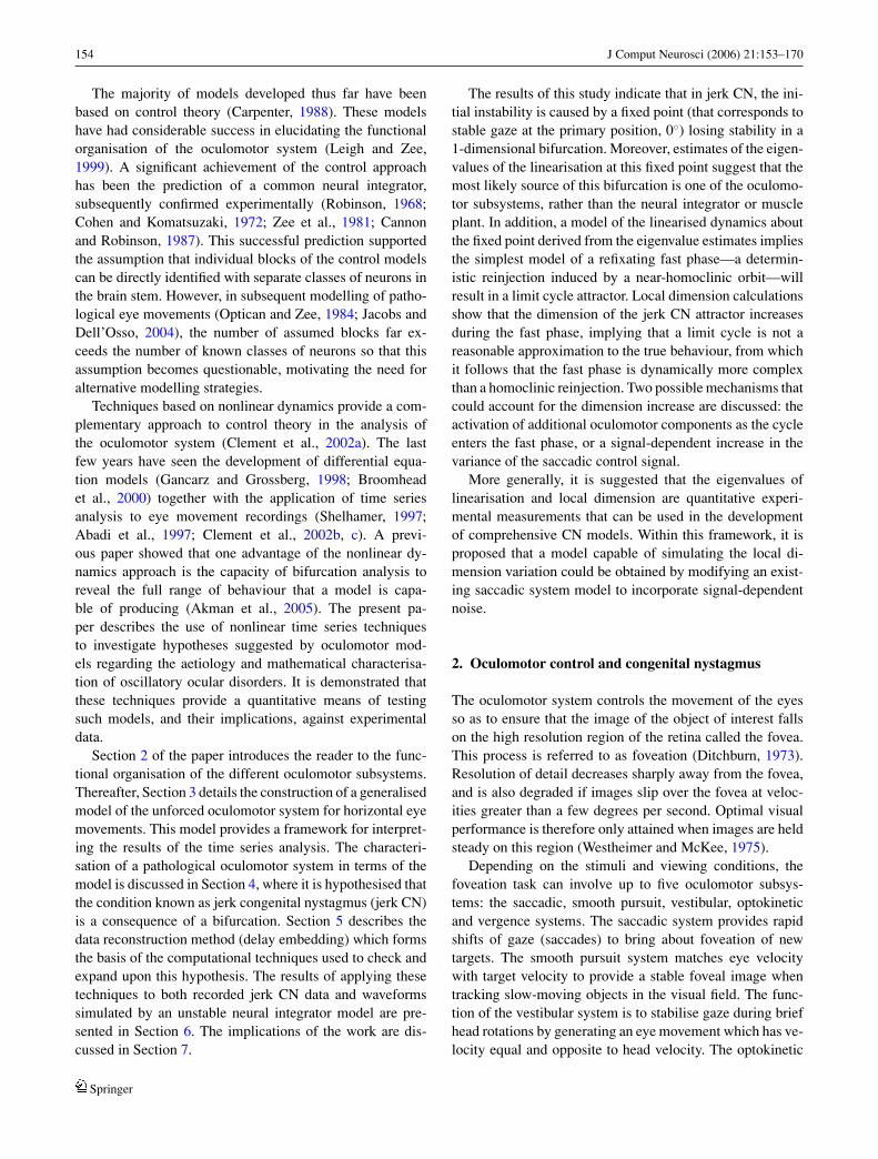
Sandikcioglu, 1975; Abadi and Worfolk, 1989; Bedell andLoshin, 1991). A common waveform observed in adultsis jerk CN, composed of an increasing exponential slowphase followed by a saccadic fast phase. The oscillationis referred to as right-beating or left-beating dependingon the direction of the fast phase. Recordings from twosubjects with left-beating jerk nystagmus can be seen inFig. 2.

3. Modelling the oculomotor control system forhorizontal eye movements: A nonlinear dynamicsapproach

Quantitative investigations of the dynamics of the muscleplant have revealed that it can be modelled as a linear systemwhich is at least second order (Robinson, 1964; Goldstein,1987). Writing x(j) for the jth time derivative of x, the mostgeneral equation describing the plant dynamics is thus

g(k) +pk−1g(k−1) + · · · + p1g + p0g

= ql(Rn(l) + b(l)

) + ql−1(Rn(l−1) + b(l−1)) + · · ·

+q1(Rn + b) + q0(Rn + b) (1)

with k ≥ 2, l ≥ 0 and q0 �= 0. Here, g is horizontal eye po-sition, n is the NI output, b = ∑

K=S,P,V,O K N ,V G bK is thesignal from the OCS (cf. Fig. 1) and R is a positive constantwhich determines the relative weighting of the position andvelocity inputs to the muscle plant.

The equation for the NI output n is

n = − 1

NTn + b

Springer


Fig. 2 Portions of eye movement recordings obtained from two subjects (A and B) with jerk nystagmus. 0o indicates gaze straight ahead (primaryposition). Positive values represent rightward movements

where the time constant NT determines the drift of the eyeback to primary position from eccentric gaze. NT is of theorder of 25 s in normal subjects (Becker and Klein, 1973).When it can be assumed that the sensory input to the ocu-lomotor subsystems is negligible (such as during viewing ofa stationary target in the primary position, or when the eyesare closed), the dynamics of each oculomotor subsystem canbe approximated by a set of autonomous, ordinary differen-tial equations. The combined dynamics of the unforced OCScan thus be written as y = f (y), where y ∈ R

q (with q a fi-nite integer) combines the state vectors of each subsystem,and f combines the corresponding vector fields. The velocitycommand b can thus be expressed as b = G(y) for somescalar function G, where G incorporates any velocity biasesthat may result in a nonzero neural integrator null position(Goldman et al., 2001).

Introducing the state vector x = (g, g, . . . , g(k−1)

)Ten-

ables the plant equation (1) to be written in the vectorisedform

x = Ax + S (n, y)

where A is the k × k matrix

A =

0 1 0 . . . 00 0 1 . . . 0...

......

. . ....

0 0 0 . . . 1−p0 −p1 −p2 . . . −pk−1

and S (n,y) = (0, . . . , 0, S (n,y))T ∈ Rk , with S(n,y) a

scalar function representing the right-hand-side of (1)expressed as a function of n and y. The final equations forthe unforced oculomotor dynamics are thus

x = Ax + S(n, y) (2)

n = − 1

NTn + G (y) (3)

y = f(y). (4)

These will sometimes be written in the condensed form z =F(z) for convenience, where z = (x, n, y) ∈ R

D , with D =k + q + 1. The equations have a skew-product form, as thevector field of (4) does not contain any terms in x and n.It follows from the form of the plant and neural integratordynamics (2)–(3) that these are slaved to the OCS dynamics(4), which determine the qualitative behaviour of the fullsystem z = F(z) (Stark, 1999).

4. Characterisation of a pathological oculomotorsystem

In terms of the modelling approach presented here, a normaloculomotor system corresponds to the unforced dynamicsz = F(z) having a single, stable fixed point z of the formz = (0, . . .0, n, y). For such a system, after motion of theeye driven by sensory input, the eye comes to rest at theprimary position. A pathological oculomotor system—suchas jerk CN—develops when z becomes unstable through abifurcation, leading to an attractor for which the eye doesnot come to rest at 0o (e.g. a stable fixed point with g �= 0, astable limit cycle, a strange attractor).1

1 The centripetal oscillations observed in some normal subjects as theyfixate a target at an eccentric gaze angle (physiological endpoint nys-tagmus) do not correspond to a pathological system by this definition,since they are driven by visual signals, rather than an endogenous insta-

Springer


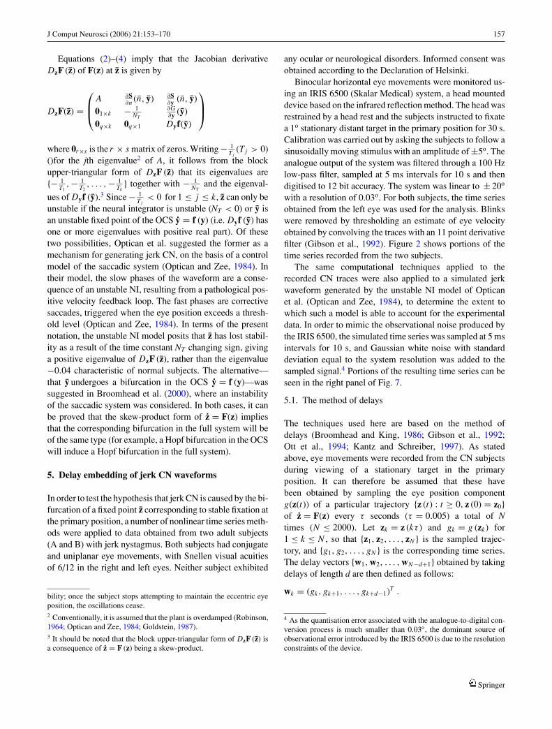
Equations (2)–(4) imply that the Jacobian derivativeDzF (z) of F(z) at z is given by

DzF(z) =

A ∂S∂n (n, y) ∂S

∂y (n, y)01×k − 1

NT

∂G∂y (y)

0q×k 0q×1 Dyf(y)

where 0r×s is the r × s matrix of zeros. Writing − 1Tj

(Tj > 0)()for the jth eigenvalue2 of A, it follows from the blockupper-triangular form of DzF (z) that its eigenvalues are{− 1

T1,− 1

T2, . . . ,− 1

Tk} together with − 1

NTand the eigenval-

ues of Dyf (y).3 Since − 1Tj

< 0 for 1 ≤ j ≤ k, z can only beunstable if the neural integrator is unstable (NT < 0) or y isan unstable fixed point of the OCS y = f (y) (i.e. Dyf (y) hasone or more eigenvalues with positive real part). Of thesetwo possibilities, Optican et al. suggested the former as amechanism for generating jerk CN, on the basis of a controlmodel of the saccadic system (Optican and Zee, 1984). Intheir model, the slow phases of the waveform are a conse-quence of an unstable NI, resulting from a pathological pos-itive velocity feedback loop. The fast phases are correctivesaccades, triggered when the eye position exceeds a thresh-old level (Optican and Zee, 1984). In terms of the presentnotation, the unstable NI model posits that z has lost stabil-ity as a result of the time constant NT changing sign, givinga positive eigenvalue of DzF (z), rather than the eigenvalue−0.04 characteristic of normal subjects. The alternative—that y undergoes a bifurcation in the OCS y = f (y)—wassuggested in Broomhead et al. (2000), where an instabilityof the saccadic system was considered. In both cases, it canbe proved that the skew-product form of z = F(z) impliesthat the corresponding bifurcation in the full system will beof the same type (for example, a Hopf bifurcation in the OCSwill induce a Hopf bifurcation in the full system).

5. Delay embedding of jerk CN waveforms

In order to test the hypothesis that jerk CN is caused by the bi-furcation of a fixed point z corresponding to stable fixation atthe primary position, a number of nonlinear time series meth-ods were applied to data obtained from two adult subjects(A and B) with jerk nystagmus. Both subjects had conjugateand uniplanar eye movements, with Snellen visual acuitiesof 6/12 in the right and left eyes. Neither subject exhibited

bility; once the subject stops attempting to maintain the eccentric eyeposition, the oscillations cease.2 Conventionally, it is assumed that the plant is overdamped (Robinson,1964; Optican and Zee, 1984; Goldstein, 1987).3 It should be noted that the block upper-triangular form of DzF (z) isa consequence of z = F (z) being a skew-product.

any ocular or neurological disorders. Informed consent wasobtained according to the Declaration of Helsinki.

Binocular horizontal eye movements were monitored us-ing an IRIS 6500 (Skalar Medical) system, a head mounteddevice based on the infrared reflection method. The head wasrestrained by a head rest and the subjects instructed to fixatea 1o stationary distant target in the primary position for 30 s.Calibration was carried out by asking the subjects to follow asinusoidally moving stimulus with an amplitude of ±5o. Theanalogue output of the system was filtered through a 100 Hzlow-pass filter, sampled at 5 ms intervals for 10 s and thendigitised to 12 bit accuracy. The system was linear to ± 20o

with a resolution of 0.03o. For both subjects, the time seriesobtained from the left eye was used for the analysis. Blinkswere removed by thresholding an estimate of eye velocityobtained by convolving the traces with an 11 point derivativefilter (Gibson et al., 1992). Figure 2 shows portions of thetime series recorded from the two subjects.

The same computational techniques applied to therecorded CN traces were also applied to a simulated jerkwaveform generated by the unstable NI model of Opticanet al. (Optican and Zee, 1984), to determine the extent towhich such a model is able to account for the experimentaldata. In order to mimic the observational noise produced bythe IRIS 6500, the simulated time series was sampled at 5 msintervals for 10 s, and Gaussian white noise with standarddeviation equal to the system resolution was added to thesampled signal.4 Portions of the resulting time series can beseen in the right panel of Fig. 7.

5.1. The method of delays

The techniques used here are based on the method ofdelays (Broomhead and King, 1986; Gibson et al., 1992;Ott et al., 1994; Kantz and Schreiber, 1997). As statedabove, eye movements were recorded from the CN subjectsduring viewing of a stationary target in the primaryposition. It can therefore be assumed that these havebeen obtained by sampling the eye position componentg(z(t)) of a particular trajectory {z (t) : t ≥ 0, z (0) = z0}of z = F(z) every τ seconds (τ = 0.005) a total of Ntimes (N ≤ 2000). Let zk = z (kτ ) and gk = g (zk) for1 ≤ k ≤ N , so that {z1, z2, . . . , zN } is the sampled trajec-tory, and {g1, g2, . . . , gN } is the corresponding time series.The delay vectors {w1, w2, . . . , wN−d+1} obtained by takingdelays of length d are then defined as follows:

wk = (gk, gk+1, . . . , gk+d−1)T .

4 As the quantisation error associated with the analogue-to-digital con-version process is much smaller than 0.03o, the dominant source ofobservational error introduced by the IRIS 6500 is due to the resolutionconstraints of the device.

Springer


It can be further assumed that asymptotically, the dy-namics of z = F(z) are confined to an attractor A lyingin an m-dimensional, smooth, compact submanifold of Rd .Letting {φt : t ∈ R} represent the flow of z = F(z), so thatz (t) = φt (z0), wk can be written as wk = � (zk) where thedelay map � : M → R

d is defined by

� (z) = (g (z) , g (φτ (z)) , . . . , g(φ(d−1)τ (z)))T .

A well-known result from applied dynamical systems the-ory, due to Takens, implies that if d ≥ 2m + 1 and certaingenericity conditions hold, � is an embedding of M in R

d ; i.e.� (M) is a smooth submanifold of R

d with � : M → � (M)a diffeomorphism (a smooth map with a smooth inverse)(Takens, 1981). The delay map therefore induces a flowψt = � ◦ φt ◦ �−1 on � (M) such that the dynamics on� (M) under ψt are equivalent to the dynamics on M underφt , up to the smooth change of coordinates �. The dynamicson M are thus reconstructed in R

d by the delay map. Indeed,many important quantities defined by φt are invariant underthe embedding. These are coordinate-independent quanti-ties, such as the dimensions of A and M, the Lyapunovexponents of the flow and the eigenvalues of linearisationat fixed points. Moreover, because wk+1 = ψτ (wk), the se-quence {w1, w2, . . . , wN−d+1} is a sampled trajectory of thereconstructed dynamics, and hence the invariant quantitiescan be recovered from the delay vectors (Broomhead andKing, 1986; Healey et al., 1991; Gibson et al., 1992; Ottet al., 1994; Kantz and Schreiber, 1997).

5.2. Choice of the delay length d

A useful tool when determining a suitable choice of thedelay length d is the global trajectory matrix X of the timeseries. X is defined as the (N − d + 1) × d matrix whosekth row is 1√

NwT

k . The singular value decomposition (SVD)of X provides information on the distribution of the delayvectors in R

d (Broomhead and King, 1985). Assuming thatthe time series is stationary with zero mean, the right singularvectors of X provide an orthonormal basis of R

d such thatin the limit N → ∞, the coordinates of the delay vectorsin the new basis are uncorrelated. Moreover, the variance ofthe jth coordinate of the delay vectors in the SVD basis isσ j

2, where σ j is the singular value of X corresponding tothe jth right singular vector (Broomhead and King, 1986).By convention, σ j ≥ σ j−1. Hence, if the first d − 1 singularvectors of X contain a significant proportion of the totalvariance (i.e.

∑d−1j=1 σ 2

j /∑d

j=1 σ 2j ≈ 1), it can be inferred

that the image of A under the delay map � lies in a d − 1dimensional linear subspace of R

d , and hence that M haseffectively been reconstructed in R

d by � (Broomhead andKing, 1985, 1986). (It should be noted that this does not

necessarily imply that � is an embedding, although this is areasonable working assumption).

For the time series of subjects A and B,∑d−1

j=1 σ 2j

/∑d

j=1 σ 2j > 0.9999 for d ≥ 7 in both cases; i.e. for d ≥ 7,

more than 99.99% of the variance lies in the first d − 1 singu-lar vectors. In view of this, d was taken equal to 7 in the subse-quent analysis of both sets of data. Applying the same analy-sis to the simulated waveform from the unstable NI model, itwas also found that

∑d−1j=1 σ 2

j /∑d

j=1 σ 2j > 0.9999 for d ≥ 7;

d was therefore set to 7 in the analysis of this data set aswell.

6. Analysis of the reconstructed attractors

This section presents the main results of the paper.Section 6.1 describes a technique for estimating fixed pointsof the reconstructed jerk CN dynamics, and shows the re-sult of carrying out this procedure on the experimental andmodel time series. Sections 6.2 and 6.3 provide a theoreticalbackground to two further techniques; computation of localattractor dimension, and estimation of eigenvalues of lineari-sation at fixed points of z = F(z). Section 6.4 gives the resultof applying these techniques to the experimental and modeldata sets in the neighbourhood of the delay vectors obtainedfrom the fixed point estimation process, and the subsequentinferences that can be made regarding the origin of the jerkinstability.

Following this, Section 6.5 details the construction of ananalytical Poincare map obtained by combining the eigen-value estimates from the experimental data with a fast phasemodelled as a homoclinic reinjection. An analysis of this mapimplies that the jerk CN attractor should be a limit cycle. Sec-tion 6.6 describes the use of local dimension calculations atdifferent points on the reconstructed data sets to determinewhether a limit cycle is a reasonable approximation to theactual behaviour.

6.1. Estimates of the reconstructed hypothetical fixedpoints

If a fixed point z of z = F(z) does exist, its image under � is afixed point of the dynamical system induced by �, and mustlie in a region where the velocity of the flow is low. Writingw = � (z), the form of � implies that w would lie on theprincipal diagonal Sp((1, . . . , 1)T ) of the delay space R

d . Areasonable estimate of w is therefore provided by the delayvector w ∈ {w1, . . . , wN−d+1} of minimum velocity lyingwithin a small distance δ of the diagonal. The upper panel ofFig. 3 shows the projection of the delay vectors for subjectB onto the first two singular vectors of the global trajectorymatrix, together with the estimate of w. The corresponding

Springer


Fig. 3 Global and local dynamics reconstructed from the time series ofsubject B using the method of delays. Upper panel. Global dynamics.Projections of the delay vectors wk onto the first two singular vectors{c1, c2} of the global trajectory matrix X. FP represents the estimatew of the hypothetical fixed point w, while the dotted line is the projec-tion of the principal diagonal of the delay space onto c1 and c2. Lowerpanel. Dynamics in the neighbourhood of the fixed point estimate. Pro-jections of wk − w onto the first two singular vectors {c1 (ε) , c2 (ε)}of the local trajectory matrix Xε (w), for the choice of ball radius ε

used to obtain the final estimate LS of the linear map governingthe dynamics in the SVD basis. {e1, e2, e3} represent the eigenvec-tors of LS; the arrows indicate the direction of the flow along theeigenvectors

plot for subject A can be seen in the left panel of Fig. 9. Forboth time series, the velocity of the reconstructed trajectoryat wk was approximated by (wk+1 − wk) /τ , and δ was setto be 1

20 th of the radius of the reconstructed attractor, asestimated by the quantity maxk ‖wk‖. The delay vector ob-tained by carrying out the same calculation on the trajectorymatrix for the model data can be seen in the left panel ofFig. 7.

6.2. Calculation of local dimension using SVD

A common tool for analysing the reconstructed attractor inthe neighbourhood of a given point w ∈ {w1, . . . , wN−d+1}is the associated local trajectory matrix (Broomhead et al.,1987; Kirby, 2000). Given ε > 0, let Bε(w) represent the setof points wk for which ‖wk − w‖ < ε; i.e. the open ball ofradius ε centred at w. Then if there are Nε points in Bε(w),the local trajectory matrix Xε(w) is defined as the Nε × dmatrix whose rows consist of the vectors 1√

Nε(wk − w)T with

wk ∈ Bε(w). The SVD of Xε (w) provides useful informationabout the geometric structure of the reconstructed data in theneighbourhood of w (Broomhead et al., 1987; Broomheadand Jones, 1989; Kirby, 2000; Hundley and Kirby, 2003).Following the notation for the global trajectory matrix, thejth singular value of Xε (w) will be written as σ j (ε) and thejth singular vector as c j (ε).

For sufficiently small ε , each vector of Bε (w) − w lies inthe tangent space Tw� (M) of the manifold � (M) at w. Also,for 1 ≤ j ≤ d, σ j (ε) is the root mean square (RMS) projec-tion of the vectors in Bε (w) − w onto c j(ε). Consequently,it is reasonable to assume that there are m singular vectorsof Xε (w) which span Tw� (M), for sufficiently small ε

(Broomhead et al., 1987; Hundley and Kirby, 2003). Writethe indices of these vectors as { j1, . . . , jm}, and the indicesof the remaining d − m vectors as { jm+1, . . . , jd}. It thenfollows that in the limit Nε → ∞ of an isotropic, uni-formly sampled neighbourhood of w, σ jk (ε) ∼ ε + O(ε2)for 1 ≤ k ≤ m and σ jk (ε) ∼ εr (k) + O(εr (k)+1) form + 1 ≤ k ≤ d, where r (k) ≥ 2. In principle, the di-mension m of M can therefore be determined by observingthe scaling behaviour of the singular values as ε is increased(Broomhead et al., 1987; Broomhead and Jones, 1989;Kirby, 2000; Hundley and Kirby, 2003).

In practice, however, noise and anisotropy of the datamodify the scaling behaviour. In particular, additive whitenoise uncorrelated with the time series causes the singularvalues which scale nonlinearly in the noise-free case to scalelinearly with ε, or to be independent of ε. What is actuallyseen depends on the size of ε relative to the magnitude of thenoise. When the data points spread beyond the extent of theball in the direction of a particular singular vector, the corre-sponding singular value scales linearly with ε. Conversely,when ε is greater than the extent of the data points in thisdirection, the corresponding singular value is independent ofε, with square approximately equal to the square of thenoise-free value plus the variance of the noise. Similarly,even in the absence of noise, if the reconstructed attractor isthin in a particular direction—due, say, to a negative Lya-punov exponent of large modulus—when ε is greater thanthe extent of the attractor in that direction, the correspond-ing singular value is independent of ε. An estimate of m is

Springer


therefore provided by the number of singular values dL thatscale linearly with ε or are constant above a level belowwhich the singular values are believed to be dominated bynoise, referred to as the noise floor (Broomhead et al., 1987;Broomhead and Jones, 1989; Healey et al., 1991). The quan-tity dL can in practice, however, both underestimate and over-estimate m, depending on factors such as noise and stronglycontracting Lyapunov exponents; it can be thought of moregenerally as the local dimension of the data at w, since itis the minimum number of degrees of freedom needed todescribe the data at that point.

6.3. Estimating eigenvalues of the linearisation at afixed point

In the case where w lies close to a fixed point w of thereconstructed dynamics, corresponding to a fixed point zof z = F(z), dL eigenvalues of DzF (z) can be estimatedfrom a linear fit of the evolution under ψτ of the projec-tions of the vectors in Bε (w) − w onto the first dL singularvectors of Xε(w) (Healey et al., 1991). This can be seeneasily in the case where the eigenvalues {λ1, . . . , λD} ofDzF (z) are real and distinct.5 Let ui be the eigenvector ofDzF (z) associated with λi , scaled to have unit norm, andwrite zk − z = ∑D

i=1 Zikui . Then for sufficiently small ε,if wk, wk+1 ∈ Bε (w), it follows from the linearisation ofz = F(z) at z and the Taylor expansion of � about z that

wk − w ≈D∑

i=1

Zik ui (5)

and

wk+1 − w ≈D∑

i=1

eλi τ Zik ui , (6)

where ui = Dz� (z) ui . Since, w ≈ w, (5) shows that eachvector of Bε (w) − w lies approximately in the linear spaceL (w) spanned by the columns of Dz� (z). It can be shownthat:

‖ui‖1 =

d−1∑

j=0

e jλi τ

|Dzg (z) ui | . (7)

(7) and (5) therefore imply that if λi < 0 with |λi | 0 or|Dzg (z) ui | ≈ 0, L (w) will be thin in the direction of ui ,in the sense that the relative variance of the data in the ui

direction will be small.

5 It is straightforward to extend this analysis to the case where DzF (z)has complex eigenvalues.

It is reasonable to assume that the thin directions will giverise to singular values of Xε(w) which have a magnitudecommensurate with the noise floor. The other directions willgive rise to singular values that scale linearly, or are constant,at values greater than the level of the noise. Relabelling thelatter directions as {u1, . . . , udL }, the points of Bε (w) − ware thus effectively confined to the dL-dimensional subspaceL (w) of L (w) spanned by {u1, . . . , udL }, with the first dL

singular vectors {c1 (ε) , . . . , cdL (ε)} of Xε (w) approximat-ing a basis for L (w). When w lies close to a fixed point ofthe dynamics, dL thus computes the number of significanteigendirections of the linearisation, which may differ fromm.

As the points of Bε (w) − w effectively lie in a propersubset of the delay space R

d , attempting to estimate eigen-values of DzF (z) directly from pairs wk − w, wk+1 − w ∈Bε (w) − w is an ill-posed numerical problem. The eigenval-ues {λ1, . . . , λdL } associated with {u1, . . . , udL } can, how-ever, be robustly estimated by projecting the points ofBε (w) − w onto L (w) (Healey et al., 1991). Define wk to bethe projection of wk − w onto the basis {c1 (ε) , . . . , cdL (ε)},so that wk = CT

ε (wk − w), where Cε is the d × dL matrixwhose jth column is c j (ε). It then follows from (5) and (6)(together with the approximation w ≈ w), that wk+1 ≈ wk ,where

= (CT

ε U)

diag{eλ1τ . . . , eλdL τ

} (CT

ε U)−1

,

and U is the d × dL matrix [u1, . . . , udL ]. Writing{µ1, . . . , µdL } for the eigenvalues of the form of

implies that λ j = 1τ

ln(µ j ) for 1 ≤ j ≤ dL . Estimates of{λ1, . . . , λdL } can therefore be obtained from an estimateof .

In practice, is estimated by collecting a subset

{(w f1 , w f1+1

), . . . ,

(w fFN

, w fFN +1)}

of the SN pairs of projected delay vectors {wk, wk+1}for which wk, wk+1 ∈ Bε (w). The approximation w f j +1 ≈w f j implies that W2 ≈ W1

T , where W1 and W2 are theFN × dL matrices with jth rows wT

f jand wT

f j +1 respectively. can therefore be estimated by finding the matrix Y whichsolves the least-squares problem minY∈RdL ×dL ‖W2 − W1Y‖2

2.By construction, W1 is full rank, giving the following least-squares estimate LS of (Barnett, 1990):

LS = (W T

2 W1) (

W T1 W1

)−1.

The remaining TN = SN − FN pairs of projected delay vec-tors are used to test the fit. These will be written as

{(wc1 , wc1+1

), . . . ,

(wcTN

, wcTN +1)}

.

Springer


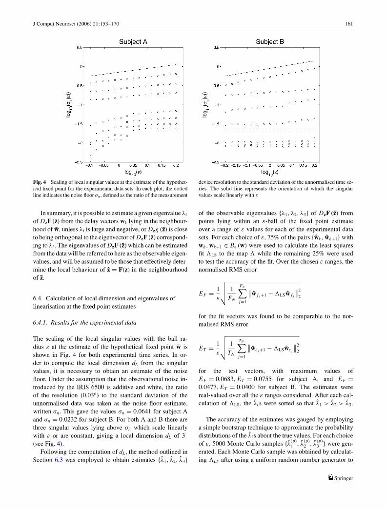
Fig. 4 Scaling of local singular values at the estimate of the hypothet-ical fixed point for the experimental data sets. In each plot, the dottedline indicates the noise floor σn , defined as the ratio of the measurement

device resolution to the standard deviation of the unnormalised time se-ries. The solid line represents the orientation at which the singularvalues scale linearly with ε

In summary, it is possible to estimate a given eigenvalue λi

of DzF (z) from the delay vectors wk lying in the neighbour-hood of w, unless λi is large and negative, or Dzg (z) is closeto being orthogonal to the eigenvector of DzF (z) correspond-ing to λi . The eigenvalues of DzF (z) which can be estimatedfrom the data will be referred to here as the observable eigen-values, and will be assumed to be those that effectively deter-mine the local behaviour of z = F(z) in the neighbourhoodof z.

6.4. Calculation of local dimension and eigenvalues oflinearisation at the fixed point estimates

6.4.1. Results for the experimental data

The scaling of the local singular values with the ball ra-dius ε at the estimate of the hypothetical fixed point w isshown in Fig. 4 for both experimental time series. In or-der to compute the local dimension dL from the singularvalues, it is necessary to obtain an estimate of the noisefloor. Under the assumption that the observational noise in-troduced by the IRIS 6500 is additive and white, the ratioof the resolution (0.03o) to the standard deviation of theunnormalised data was taken as the noise floor estimate,written σn . This gave the values σn = 0.0641 for subject Aand σn = 0.0232 for subject B. For both A and B there arethree singular values lying above σn which scale linearlywith ε or are constant, giving a local dimension dL of 3(see Fig. 4).

Following the computation of dL, the method outlined inSection 6.3 was employed to obtain estimates {λ1, λ2, λ3}

of the observable eigenvalues {λ1, λ2, λ3} of DzF (z) frompoints lying within an ε-ball of the fixed point estimateover a range of ε values for each of the experimental datasets. For each choice of ε, 75% of the pairs {wk, wk+1} withwk, wk+1 ∈ Bε (w) were used to calculate the least-squaresfit LS to the map while the remaining 25% were usedto test the accuracy of the fit. Over the chosen ε ranges, thenormalised RMS error

EF = 1

ε

√√√√ 1

FN

FN∑

j=1

∥∥w f j +1 − LSw f j

∥∥22

for the fit vectors was found to be comparable to the nor-malised RMS error

ET = 1

ε

√√√√ 1

TN

TN∑

j=1

∥∥wc j +1 − LSwc j

∥∥22

for the test vectors, with maximum values ofEF = 0.0683, ET = 0.0755 for subject A, and EF =0.0477, ET = 0.0400 for subject B. The estimates werereal-valued over all the ε ranges considered. After each cal-culation of LS, the λi s were sorted so that λ1 > λ2 > λ3.

The accuracy of the estimates was gauged by employinga simple bootstrap technique to approximate the probabilitydistributions of the λi s about the true values. For each choiceof ε, 5000 Monte Carlo samples {λ(p)

1 , λ(p)2 , λ

(p)3 } were gen-

erated. Each Monte Carlo sample was obtained by calculat-ing LS after using a uniform random number generator to

Springer


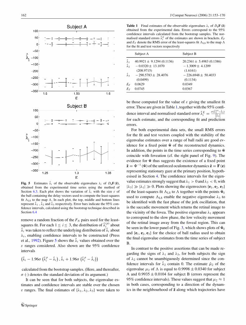
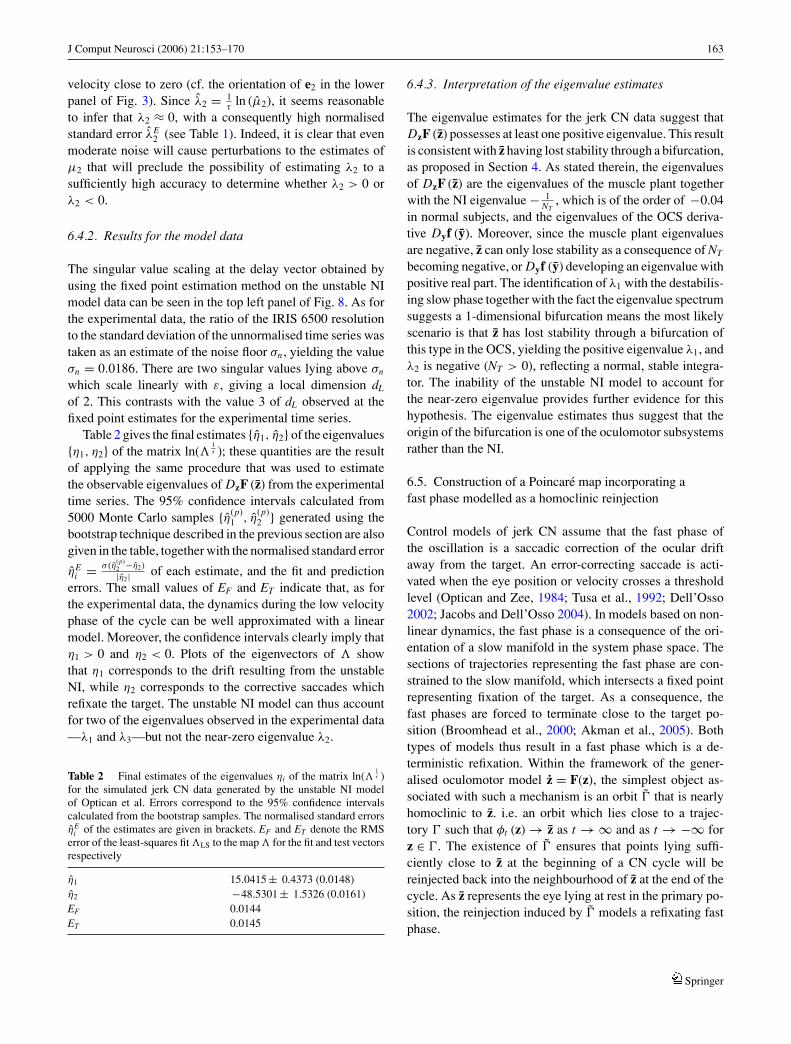
Fig. 5 Estimates λi of the observable eigenvalues λi of DzF (z),obtained from the experimental time series using the method ofSection 6.3. Each plot shows the variation of λi with the size ε ofthe ball containing the delay vectors used to compute the least-squaresfit LS to the map . In each plot, the top, middle and bottom linesrepresent λ1 , λ2 and λ3 respectively. Error bars indicate the 95% con-fidence intervals, calculated using the bootstrap technique described inSection 6.4

remove a random fraction of the FN pairs used for the least-squares fit. For each 1 ≤ i ≤ 3, the distribution of λ

(p)i about

λi was taken to reflect the underlying distribution of λi aboutλi , enabling confidence intervals to be constructed (Presset al., 1992). Figure 5 shows the λi values obtained over theε ranges considered. Also shown are the 95% confidenceintervals(λi − 1.96σ

(λ

pi − λi

), λi + 1.96σ

(λ

pi − λi

))

calculated from the bootstrap samples. (Here, and thereafter,σ (·) denotes the standard deviation of its argument.)

It can be seen that for both subjects, the eigenvalue es-timates and confidence intervals are stable over the chosenε ranges. The final estimates of {λ1, λ2, λ3} were taken to

Table 1 Final estimates of the observable eigenvalues λi of DzF (z)obtained from the experimental data. Errors correspond to the 95%confidence intervals calculated from the bootstrap samples. The nor-malised standard errors λE

i of the estimates are shown in brackets. EF

and ET denote the RMS error of the least-squares fit LS to the map

for the fit and test vectors respectively

Subject A Subject B

λ1 40.9921 ± 9.1294 (0.1136) 20.2361 ± 5.4983 (0.1386)λ2 − 0.0320 ± 13.1070

(208.9715)− 1.3009 ± 4.1209(1.6161)

λ3 − 290.5783 ± 28.4076(0.0499)

− 226.6948 ± 50.4033(0.1134)

EF 0.0629 0.0349ET 0.0745 0.0367

be those computed for the value of ε giving the smallest fiterror. These are given in Table 1, together with the 95% confi-

dence interval and normalised standard error λEi = σ (λ(p)

2 −λ2)

|λ2|for each estimate, and the corresponding fit and predictionerrors.

For both experimental data sets, the small RMS errorsfor the fit and test vectors coupled with the stability of theeigenvalue estimates over a range of ball radii are good ev-idence for a fixed point w of the reconstructed dynamics.In addition, the points in the time series corresponding to wcoincide with foveation (cf. the right panel of Fig. 9). Theevidence for w thus suggests the existence of a fixed pointz = �−1 (w) of the unforced oculomotor dynamics z = F (z)representing stationary gaze at the primary position, hypoth-esised in Section 4. The confidence intervals for the eigen-value estimates strongly suggest that λ1 > 0 and λ3 < 0, with|λ3| |λ1| 0. Plots showing the eigenvectors {e1, e2, e3}of the least-squares fit LS to together with the points wk

used to compute LS enable the negative eigenvalue λ3 tobe identified with the fast phase of the jerk oscillation, thatis the saccadic movement which returns the retinal image tothe vicinity of the fovea. The positive eigenvalue λ1 appearsto correspond to the slow phase, the low velocity movementof the retinal image away from the foveal region. This canbe seen in the lower panel of Fig. 3, which shows plots of wk

and {e1, e2, e3} for the choice of ball radius used to obtainthe final eigenvalue estimates from the time series of subjectB.

In contrast to the positive assertions that can be made re-garding the signs of λ1 and λ3, for both subjects the signof λ2 cannot be unambiguously determined since the con-fidence intervals for λ2 contain 0. The estimate µ2 of theeigenvalue µ2 of is equal to 0.9998 ± 0.0340 for subjectA and 0.9935 ± 0.0104 for subject B (errors represent the95% confidence intervals). These values suggest that µ2 ≈ 1in both cases, corresponding to a direction of the dynam-ics in the neighbourhood of z along which trajectories have

Springer


velocity close to zero (cf. the orientation of e2 in the lowerpanel of Fig. 3). Since λ2 = 1

τln (µ2), it seems reasonable

to infer that λ2 ≈ 0, with a consequently high normalisedstandard error λE

2 (see Table 1). Indeed, it is clear that evenmoderate noise will cause perturbations to the estimates ofµ2 that will preclude the possibility of estimating λ2 to asufficiently high accuracy to determine whether λ2 > 0 orλ2 < 0.

6.4.2. Results for the model data

The singular value scaling at the delay vector obtained byusing the fixed point estimation method on the unstable NImodel data can be seen in the top left panel of Fig. 8. As forthe experimental data, the ratio of the IRIS 6500 resolutionto the standard deviation of the unnormalised time series wastaken as an estimate of the noise floor σn , yielding the valueσn = 0.0186. There are two singular values lying above σn

which scale linearly with ε, giving a local dimension dL

of 2. This contrasts with the value 3 of dL observed at thefixed point estimates for the experimental time series.

Table 2 gives the final estimates {η1, η2} of the eigenvalues{η1, η2} of the matrix ln(

1τ ); these quantities are the result

of applying the same procedure that was used to estimatethe observable eigenvalues of DzF (z) from the experimentaltime series. The 95% confidence intervals calculated from5000 Monte Carlo samples {η(p)

1 , η(p)2 } generated using the

bootstrap technique described in the previous section are alsogiven in the table, together with the normalised standard error

ηEi = σ (η(p)

2 −η2)|η2| of each estimate, and the fit and prediction

errors. The small values of EF and ET indicate that, as forthe experimental data, the dynamics during the low velocityphase of the cycle can be well approximated with a linearmodel. Moreover, the confidence intervals clearly imply thatη1 > 0 and η2 < 0. Plots of the eigenvectors of showthat η1 corresponds to the drift resulting from the unstableNI, while η2 corresponds to the corrective saccades whichrefixate the target. The unstable NI model can thus accountfor two of the eigenvalues observed in the experimental data—λ1 and λ3—but not the near-zero eigenvalue λ2.

Table 2 Final estimates of the eigenvalues ηi of the matrix ln(1τ )

for the simulated jerk CN data generated by the unstable NI modelof Optican et al. Errors correspond to the 95% confidence intervalscalculated from the bootstrap samples. The normalised standard errorsηE

i of the estimates are given in brackets. EF and ET denote the RMSerror of the least-squares fit LS to the map for the fit and test vectorsrespectively

η1 15.0415 ± 0.4373 (0.0148)η2 −48.5301 ± 1.5326 (0.0161)EF 0.0144ET 0.0145

6.4.3. Interpretation of the eigenvalue estimates

The eigenvalue estimates for the jerk CN data suggest thatDzF (z) possesses at least one positive eigenvalue. This resultis consistent with z having lost stability through a bifurcation,as proposed in Section 4. As stated therein, the eigenvaluesof DzF (z) are the eigenvalues of the muscle plant togetherwith the NI eigenvalue − 1

NT, which is of the order of −0.04

in normal subjects, and the eigenvalues of the OCS deriva-tive Dyf (y). Moreover, since the muscle plant eigenvaluesare negative, z can only lose stability as a consequence of NT

becoming negative, or Dyf (y) developing an eigenvalue withpositive real part. The identification of λ1 with the destabilis-ing slow phase together with the fact the eigenvalue spectrumsuggests a 1-dimensional bifurcation means the most likelyscenario is that z has lost stability through a bifurcation ofthis type in the OCS, yielding the positive eigenvalue λ1, andλ2 is negative (NT > 0), reflecting a normal, stable integra-tor. The inability of the unstable NI model to account forthe near-zero eigenvalue provides further evidence for thishypothesis. The eigenvalue estimates thus suggest that theorigin of the bifurcation is one of the oculomotor subsystemsrather than the NI.

6.5. Construction of a Poincare map incorporating afast phase modelled as a homoclinic reinjection

Control models of jerk CN assume that the fast phase ofthe oscillation is a saccadic correction of the ocular driftaway from the target. An error-correcting saccade is acti-vated when the eye position or velocity crosses a thresholdlevel (Optican and Zee, 1984; Tusa et al., 1992; Dell’Osso2002; Jacobs and Dell’Osso 2004). In models based on non-linear dynamics, the fast phase is a consequence of the ori-entation of a slow manifold in the system phase space. Thesections of trajectories representing the fast phase are con-strained to the slow manifold, which intersects a fixed pointrepresenting fixation of the target. As a consequence, thefast phases are forced to terminate close to the target po-sition (Broomhead et al., 2000; Akman et al., 2005). Bothtypes of models thus result in a fast phase which is a de-terministic refixation. Within the framework of the gener-alised oculomotor model z = F(z), the simplest object as-sociated with such a mechanism is an orbit � that is nearlyhomoclinic to z. i.e. an orbit which lies close to a trajec-tory � such that φt (z) → z as t → ∞ and as t → −∞ forz ∈ �. The existence of � ensures that points lying suffi-ciently close to z at the beginning of a CN cycle will bereinjected back into the neighbourhood of z at the end of thecycle. As z represents the eye lying at rest in the primary po-sition, the reinjection induced by � models a refixating fastphase.

Springer


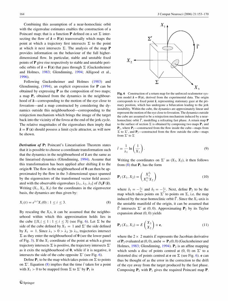
Combining this assumption of a near-homoclinic orbitwith the eigenvalue estimates enables the construction of aPoincare map; that is a function P defined on a set inter-secting the flow of z = F(z) transversally which maps thepoint at which a trajectory first intersects to the pointat which it next intersects . The analysis of the map Pprovides information on the behaviour of the full higher-dimensional flow. In particular, stable and unstable fixedpoints of P give rise respectively to stable and unstable peri-odic orbits of z = F(z) that pass through (Guckenheimerand Holmes, 1983; Glendinning, 1994; Alligood et al.,1996).

Following Guckenheimer and Holmes (1983) andGlendinning, (1994), an explicit expression for P can beobtained by expressing P as the composition of two maps;a map P1 obtained from the dynamics in the neighbour-hood of z—corresponding to the motion of the eye close tofoveation—and a map constructed by considering the dy-namics outside this neighbourhood—corresponding to thereinjection mechanism which brings the image of the targetback into the vicinity of the fovea at the end of the jerk cycle.The relative magnitudes of the eigenvalues then imply thatz = F (z) should possess a limit cycle attractor, as will nowbe shown.

Derivation of P: Poincare’s Linearisation Theorem statesthat it is possible to choose a coordinate transformation suchthat the dynamics in the neighbourhood of z are the same asthe linearised dynamics (Glendinning, 1994). Assume thatthis transformation has been applied after shifting z to theorigin 0. The flow in the neighbourhood of 0 can then be ap-proximated by the flow in the 3-dimensional space spannedby the eigenvectors of the transformed vector field associ-ated with the observable eigenvalues {λ1, λ2, λ3} of DzF (z).Writing (X1, X2, X3) for the coordinates in the eigenvectorbasis, the dynamics are thus given by:

Xi (t) = eλi t Xi (0) : 1 ≤ i ≤ 3. (8)

By rescaling the Xis, it can be assumed that the neighbo-urhood within which this approximation holds lies inthe cube {|Xi | ≤ 1 : 1 ≤ i ≤ 3} (see Fig. 6). Let be theside of the cube defined by X3 = 1 and ′ the side definedby X1 = 1. Since λ1 > 0 > λ2 λ3, trajectories intersect as they enter the neighbourhood of 0 (see the lower panelof Fig. 3). If the X1 coordinate of the point at which a giventrajectory intersects is positive, the trajectory intersects ′

as it exits the neighbourhood of 0, while if it is negative, itintersects the side of the cube opposite ′ (see Fig. 6).

Define P1 to be the map which takes points on to pointson ′. Equation (8) implies that the time t taken for a pointwith X1 > 0 to be mapped from to ′ by P1 is

Fig. 6 Construction of a return map for the unforced oculomotor sys-tem model z = F(z), derived from the experimental data. The origincorresponds to a fixed point z, representing stationary gaze at the pri-mary position, which has undergone a bifurcation leading to the jerkinstability. Within the cube, the dynamics are approximately linear andrepresent the motion of the eye close to foveation. The dynamics outsidethe cube are assumed to be a reinjection mechanism induced by a near-homoclinic orbit �, modelling a refixating fast phase. A return map Pto the surface of section is obtained by composing two maps P1 andP2, where P1—constructed from the flow inside the cube—maps from to ′, and P2—constructed from the flow outside the cube—mapsfrom ′ to

t = 1

λ1ln

(1

X1

). (9)

Writing the coordinates on ′ as (X3, X2), it then followsfrom (8) that P1 has the form

P1 (X1, X2) =(

X δ11

X δ21 X2

)(10)

where δ1 = − λ3λ1

and δ2 = − λ2λ1

. Next, define P2 to be themap which takes points on ′ to points on , i.e. the mapinduced by the near-homoclinic orbit �. Since the X1-axis isthe unstable manifold of the origin, it can be assumed that� intersects ′ at (0, 0). Approximating P2 by its Taylorexpansion about (0, 0) yields

P2 (X3, X2) = E

(X3

X2

)+ e, (11)

where the 2 × 2 matrix E represents the Jacobian derivativeof P2 evaluated at (0, 0), and e = P2(0, 0) (Guckenheimer andHolmes, 1983; Glendinning, 1994). P2 is an affine mappingwhich sends a disc of points centred at (0, 0) on ′ to adistorted disc of points centred at e on (see Fig. 6). e canthus be thought of as the error in the correction to the driftof the eye away from the target produced by the fast phase.Composing P2 with P1 gives the required Poincare map P.

Springer


Substituting (10) and (11) into P = P2 ◦ P1 leads to theexpression below:

P (X1, X2) = E

(X δ1

1

X δ21 X2

)+ e.

Simplification of P: Using the fact that the time-of-flight t isbounded enables P to be simplified. t must be bounded aboveby some value t2, reflecting the minimum frequency of thenystagmus, and bounded below by some value t1, reflectingthe minimum residency time of the target image in the fovealregion. Writing α = e−λ1t2 and β = e−λ1t1 , (9) implies that onthe domain of P, α ≤ X1 ≤ β and hence αδ2 ≤ X δ2

1 ≤ βδ2 .Computing t1 and t2 from the time series gives the valuesα = 0.0040, β = 0.4405 for subject A, and α = 0.0392, β =0.4925 for subject B (Akman, 2000). Setting λ2 equal to− 1

NTwith the standard NI time constant of 25 s yields δ2 =

9.7580 × 10−4 for A, and δ2 = 19.7667 × 10−4 for B. Forboth subjects, these values imply αδ2 , βδ2 ≈ 1. This givesX δ2

1 ≈ 1, whence the final approximation

P (X1, X2) = E

(X δ1

1X2

)+ e. (12)

Defining X = (X1, X2)T and p(X

) = (X δ11 , X2)T enables

(12) to be written in the vectorised form

P (X) = Ep (X) + e. (13)

Analysis of P: As P is a return map, it must map points in itsdomain back onto . This places restrictions on E which canbe used to deduce that P is a contraction mapping on a closedsubset of its domain. The condition on P can be expressedas ‖P (X)‖∞ ≤ 1 for all X in the domain of P, where ‖·‖∞represents the vector and matrix infinity norm. Equation (13)implies

‖P(X)‖∞ ≤ ‖E‖∞‖p(X)‖∞ + ‖e‖∞

≤ ‖E‖∞ maxX∈ ,α≤X1≤β

‖p(X)‖∞ + ‖e‖∞.

By definition, ‖p (X)‖∞ = max{|X δ11 |, |X2|}. Since −λ3

λ1, δ1 > 1 and thus for X ∈ with α ≤ X1 ≤ β, |X δ11 | ≤

βδ1 < 1. As |X2| ≤ 1 on , maxX∈ ,α≤X1≤β ‖p (X)‖∞ = 1.A minimally sufficient condition for P to map its domaininto is therefore ‖E‖∞ ≤ 1 − ‖e‖∞.

So now let X = (X1, X2)T and X′ = (X ′1, X ′

2)T lie in thedomain of P. Then by (13),

P (X) − P(X′) = E(p (X) − p(X′)).

Using the Mean Value Theorem, the expression above canbe written as

P(X) − P(X′) = E J (ξ )(X − X′)

where J(ξ ) is the Jacobian derivative of p evaluated at apoint ξ = (ξ1, ξ2)T lying on the line segment between X andX′. J (ξ ) = diag{δ1ξ

δ1−11 , 1}, and so the expression above

implies

‖P(X)−P(X′)‖∞ ≤‖E‖∞ max{δ1ξ

δ1−11 , 1

}‖X − X′‖∞

≤ (1− ‖e‖∞)max{δ1β

δ1−1, 1}‖X − X′‖∞.

The eigenvalue ratio δ1 has the value 7.0886 for subject Aand 11.2025 for subject B, giving δ1β

δ1−1 = 0.0482 for Aand δ1β

δ1−1 = 0.0081 for B. Hence, max{δ1βδ1−1, 1} = 1 in

both cases, leading to the final inequality

‖P (X) − P(X′)‖∞ ≤ (1 − ‖e‖∞) ‖X − X′‖∞.

Finally, let be the largest closed subset of the domainof P such that P

(

) ⊆ . Since 0 < 1 − ‖e‖∞ < 1, P isa contraction mapping on , and so has a unique, globallyattracting fixed point in this set. It follows that there is anattracting periodic orbit of z = F(z) in a tubular neighbour-hood of �. The attractor A of z = F (z) should therefore bea limit cycle, giving a periodic eye position time series.

6.6. Calculation of local dimension around the jerk CNcycle

The simplest attractor A of z = F(z) that could produceoscillatory behaviour is a stable limit cycle; indeed it wasargued in the last section that a fast phase comprising ahomoclinic refixation will lead to an attractor of this type.For such an attractor, the manifold M containingA isA itself,and so the dimension m of M is 1. It therefore follows from thediscussion of Sections 6.2 and 6.3 that for both experimentaldata sets, dL should equal 1 on the reconstructed trajectory,except at points in the vicinity of the reconstructed fixedpoint w, where dL reflects the dimension of the lineariseddynamics rather than of M. Since, the local dimension is 3at w (see Fig. 4), dL should therefore decrease towards 1 asthe trajectory leaves the neighbourhood of w during the slowphase, before increasing back to 3 towards the end of thefast phase as the trajectory reenters the vicinity of the fixedpoint. Indeed, a variation in dL of this type was observedfor the unstable NI model data, for which the underlyingattractor is periodic (Optican and Zee, 1984). Figure 7 shows3 points of the reconstructed attractor bounded away fromthe foveation region at which dL was computed. The scaling

Springer


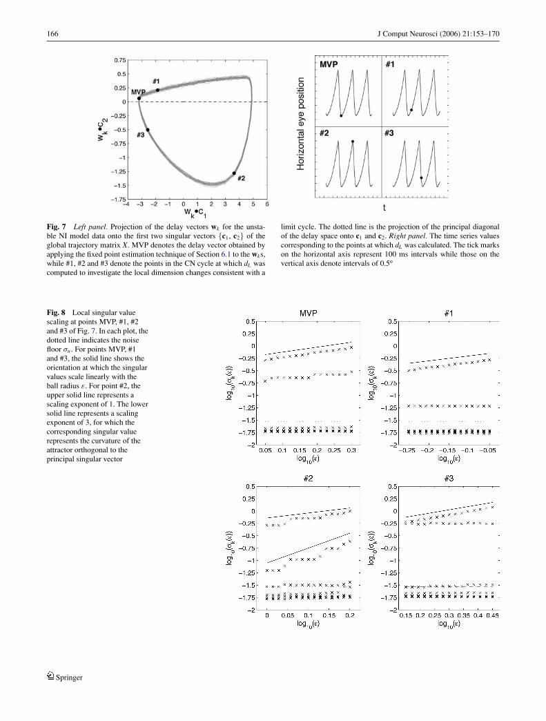
Fig. 7 Left panel. Projection of the delay vectors wk for the unsta-ble NI model data onto the first two singular vectors {c1, c2} of theglobal trajectory matrix X. MVP denotes the delay vector obtained byapplying the fixed point estimation technique of Section 6.1 to the wks,while #1, #2 and #3 denote the points in the CN cycle at which dL wascomputed to investigate the local dimension changes consistent with a

limit cycle. The dotted line is the projection of the principal diagonalof the delay space onto c1 and c2. Right panel. The time series valuescorresponding to the points at which dL was calculated. The tick markson the horizontal axis represent 100 ms intervals while those on thevertical axis denote intervals of 0.5o

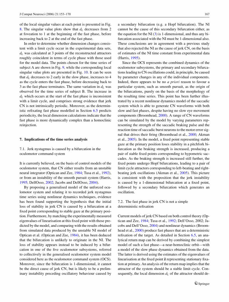
Fig. 8 Local singular valuescaling at points MVP, #1, #2and #3 of Fig. 7. In each plot, thedotted line indicates the noisefloor σn . For points MVP, #1and #3, the solid line shows theorientation at which the singularvalues scale linearly with theball radius ε. For point #2, theupper solid line represents ascaling exponent of 1. The lowersolid line represents a scalingexponent of 3, for which thecorresponding singular valuerepresents the curvature of theattractor orthogonal to theprincipal singular vector

Springer


of the local singular values at each point is presented in Fig.8. The singular value plots show that dL decreases from 2at foveation to 1 at the beginning of the fast phase, beforeincreasing back to 2 at the end of the fast phase.

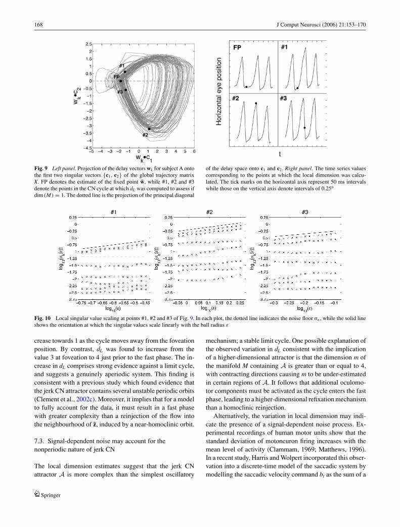
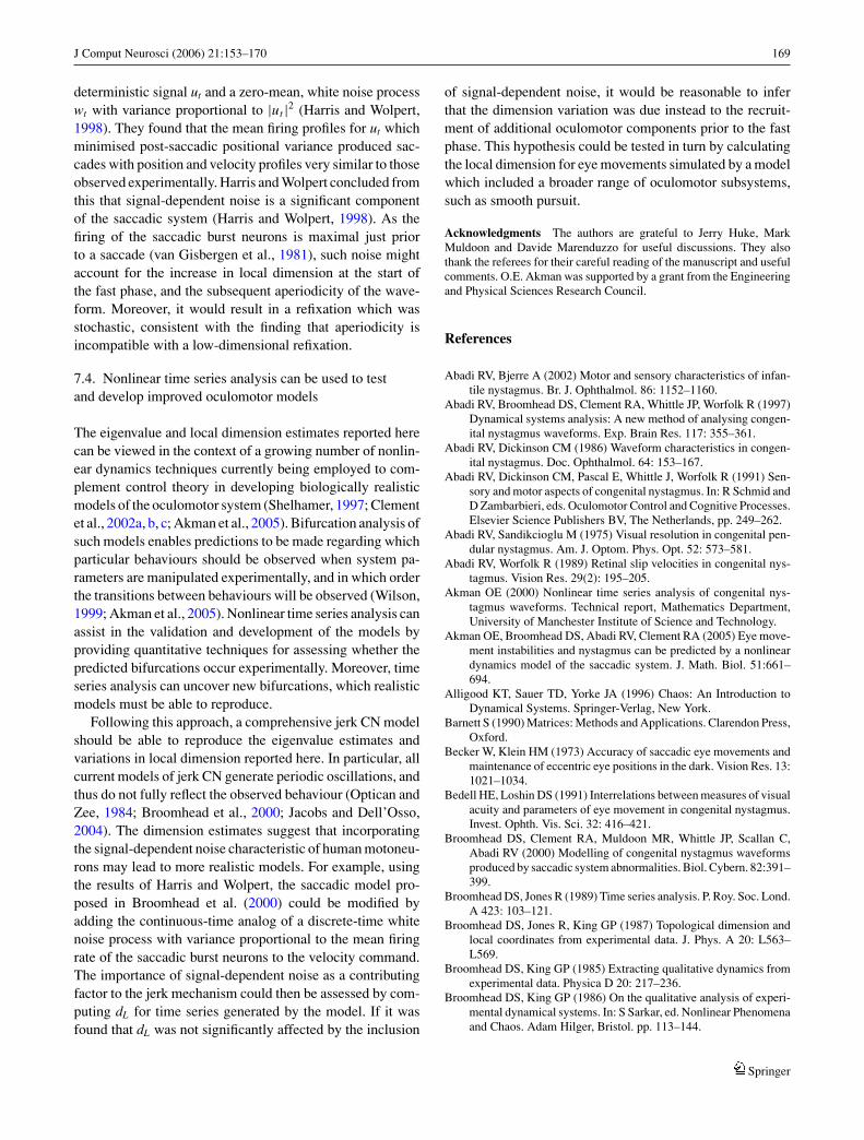
In order to determine whether dimension changes consis-tent with a limit cycle occur in the experimental data sets,dL was calculated at 3 points of the reconstructed attractorsroughly coincident in terms of cycle phase with those usedfor the model data. The points chosen for the time series ofsubject A are shown in Fig. 9, while the corresponding localsingular value plots are presented in Fig. 10. It can be seenthat dL decreases to 2 early in the slow phase, increases to 4as the cycle enters the fast phase, before decreasing back to3 as the fast phase terminates. The same variation in dL wasobserved for the time series of subject B. The increase indL which occurs at the start of the fast phase is inconsistentwith a limit cycle, and comprises strong evidence that jerkCN is not intrinsically periodic. Moreover, as the determin-istic refixating fast phase modelled in Section 6.5 predictsperiodicity, the local dimension calculations indicate that thefast phase is more dynamically complex than a homoclinicreinjection.

7. Implications of the time series analysis

7.1. Jerk nystagmus is caused by a bifurcation in theoculomotor command system

It is currently believed, on the basis of control models of theoculomotor system, that CN either results from an unstableneural integrator (Optican and Zee, 1984; Tusa et al., 1992),or from an instability of the smooth pursuit system (Harris,1995; DellOsso, 2002; Jacobs and DellOsso, 2004).

By proposing a generalised model of the unforced ocu-lomotor system and relating it to recorded jerk nystagmustime series using nonlinear dynamics techniques, evidencehas been found supporting the hypothesis that the initialloss of stability in jerk CN is caused by a bifurcation at afixed point corresponding to stable gaze at the primary posi-tion. Furthermore, by matching the experimentally measuredeigenvalues of linearisation at this fixed point with those pre-dicted by the model, and comparing with the results obtainedfrom simulated data produced by the unstable NI model ofOptican et al. (Optican and Zee, 1984), it has been deducedthat the bifurcation is unlikely to originate in the NI. Theloss of stability appears instead to be induced by a bifur-cation in one of the five oculomotor subsystems, referredto collectively in the generalised oculomotor system modelconsidered here as the oculomotor command system (OCS).Moreover, since the bifurcation is 1-dimensional, it cannotbe the direct cause of jerk CN, but is likely to be a prelim-inary instability preceding oscillatory behaviour caused by

a secondary bifurcation (e.g. a Hopf bifurcation). The NIcannot be the cause of this secondary bifurcation either, asthe equation for the NI (3) is 1-dimensional, and thus any bi-furcation associated with the NI must be 1-dimensional also.These conclusions are in agreement with a previous studythat also rejected the NI as the cause of jerk CN, on the basisof estimates of the NI time constant from experimental data(Harris, 1995).

Since the OCS represents the combined dynamics of theoculomotor subsystems, the primary and secondary bifurca-tions leading to CN oscillations could, in principle, be causedby parameter changes in any of the individual components.Indeed, there appears to be no a priori reason to favour aparticular system, such as smooth pursuit, as the origin ofthe bifurcations, purely on the basis of the morphology ofthe resulting time series. This point has been further illus-trated by a recent nonlinear dynamics model of the saccadicsystem which is able to generate CN waveforms with bothslow and fast phases, despite having no slow eye movementcomponents (Broomhead, 2000). A range of CN waveformscan be simulated by the model by varying parameters rep-resenting the strength of the saccadic braking pulse and thereaction time of saccadic burst neurons to the motor error sig-nal that drives their firing (Broomhead et al., 2000; Akmanet al., 2005). In the model, a fixed point representing stablegaze at the primary position loses stability in a pitchfork bi-furcation as the braking strength is increased, producing apair of stable fixed points corresponding to hypometric sac-cades. As the braking strength is increased still further, thefixed points undergo Hopf bifurcations, leading to a pair oflimit cycle attractors corresponding to left-beating and right-beating jerk oscillations (Akman et al., 2005). This pictureis consistent with the proposition that the jerk instabilityis caused by a 1-dimensional bifurcation at a fixed point,followed by a secondary bifurcation which generates anoscillation.

7.2. The fast phase in jerk CN is not a simpledeterministic refixation

Current models of jerk CN based on both control theory (Op-tican and Zee, 1984; Tusa et al., 1992; Dell’Osso, 2002; Ja-cobs and Dell’Osso, 2004) and nonlinear dynamics (Broom-head et al., 2000) produce fast phases that are a deterministicrefixation of the target. As detailed in Section 6.5, an ana-lytical return map can be derived by combining the simplestmodel of such a fast phase—a near-homoclinic orbit—witha model of the slow phase dynamics obtained from the data.The latter is derived using the estimates of the eigenvalues oflinearisation at the fixed point z representing stationary fixa-tion at primary. An analysis of the return map implies that theattractor of the system should be a stable limit cycle. Con-sequently, the local dimension dL of the attractor should de-

Springer


Fig. 9 Left panel. Projection of the delay vectors wk for subject A ontothe first two singular vectors {c1, c2} of the global trajectory matrixX. FP denotes the estimate of the fixed point w, while #1, #2 and #3denote the points in the CN cycle at which dL was computed to assess ifdim (M) = 1. The dotted line is the projection of the principal diagonal

of the delay space onto c1 and c2. Right panel. The time series valuescorresponding to the points at which the local dimension was calcu-lated. The tick marks on the horizontal axis represent 50 ms intervalswhile those on the vertical axis denote intervals of 0.25o

Fig. 10 Local singular value scaling at points #1, #2 and #3 of Fig. 9. In each plot, the dotted line indicates the noise floor σn , while the solid lineshows the orientation at which the singular values scale linearly with the ball radius ε

crease towards 1 as the cycle moves away from the foveationposition. By contrast, dL was found to increase from thevalue 3 at foveation to 4 just prior to the fast phase. The in-crease in dL comprises strong evidence against a limit cycle,and suggests a genuinely aperiodic system. This finding isconsistent with a previous study which found evidence thatthe jerk CN attractor contains several unstable periodic orbits(Clement et al., 2002c). Moreover, it implies that for a modelto fully account for the data, it must result in a fast phasewith greater complexity than a reinjection of the flow intothe neighbourhood of z, induced by a near-homoclinic orbit.

7.3. Signal-dependent noise may account for thenonperiodic nature of jerk CN

The local dimension estimates suggest that the jerk CNattractor A is more complex than the simplest oscillatory

mechanism; a stable limit cycle. One possible explanation ofthe observed variation in dL consistent with the implicationof a higher-dimensional attractor is that the dimension m ofthe manifold M containing A is greater than or equal to 4,with contracting directions causing m to be under-estimatedin certain regions of A. It follows that additional oculomo-tor components must be activated as the cycle enters the fastphase, leading to a higher-dimensional refixation mechanismthan a homoclinic reinjection.

Alternatively, the variation in local dimension may indi-cate the presence of a signal-dependent noise process. Ex-perimental recordings of human motor units show that thestandard deviation of motoneuron firing increases with themean level of activity (Clammam, 1969; Matthews, 1996).In a recent study, Harris and Wolpert incorporated this obser-vation into a discrete-time model of the saccadic system bymodelling the saccadic velocity command bt as the sum of a

Springer


deterministic signal ut and a zero-mean, white noise processwt with variance proportional to |ut |2 (Harris and Wolpert,1998). They found that the mean firing profiles for ut whichminimised post-saccadic positional variance produced sac-cades with position and velocity profiles very similar to thoseobserved experimentally. Harris and Wolpert concluded fromthis that signal-dependent noise is a significant componentof the saccadic system (Harris and Wolpert, 1998). As thefiring of the saccadic burst neurons is maximal just priorto a saccade (van Gisbergen et al., 1981), such noise mightaccount for the increase in local dimension at the start ofthe fast phase, and the subsequent aperiodicity of the wave-form. Moreover, it would result in a refixation which wasstochastic, consistent with the finding that aperiodicity isincompatible with a low-dimensional refixation.

7.4. Nonlinear time series analysis can be used to testand develop improved oculomotor models

The eigenvalue and local dimension estimates reported herecan be viewed in the context of a growing number of nonlin-ear dynamics techniques currently being employed to com-plement control theory in developing biologically realisticmodels of the oculomotor system (Shelhamer, 1997; Clementet al., 2002a, b, c; Akman et al., 2005). Bifurcation analysis ofsuch models enables predictions to be made regarding whichparticular behaviours should be observed when system pa-rameters are manipulated experimentally, and in which orderthe transitions between behaviours will be observed (Wilson,1999; Akman et al., 2005). Nonlinear time series analysis canassist in the validation and development of the models byproviding quantitative techniques for assessing whether thepredicted bifurcations occur experimentally. Moreover, timeseries analysis can uncover new bifurcations, which realisticmodels must be able to reproduce.

Following this approach, a comprehensive jerk CN modelshould be able to reproduce the eigenvalue estimates andvariations in local dimension reported here. In particular, allcurrent models of jerk CN generate periodic oscillations, andthus do not fully reflect the observed behaviour (Optican andZee, 1984; Broomhead et al., 2000; Jacobs and Dell’Osso,2004). The dimension estimates suggest that incorporatingthe signal-dependent noise characteristic of human motoneu-rons may lead to more realistic models. For example, usingthe results of Harris and Wolpert, the saccadic model pro-posed in Broomhead et al. (2000) could be modified byadding the continuous-time analog of a discrete-time whitenoise process with variance proportional to the mean firingrate of the saccadic burst neurons to the velocity command.The importance of signal-dependent noise as a contributingfactor to the jerk mechanism could then be assessed by com-puting dL for time series generated by the model. If it wasfound that dL was not significantly affected by the inclusion

of signal-dependent noise, it would be reasonable to inferthat the dimension variation was due instead to the recruit-ment of additional oculomotor components prior to the fastphase. This hypothesis could be tested in turn by calculatingthe local dimension for eye movements simulated by a modelwhich included a broader range of oculomotor subsystems,such as smooth pursuit.

Acknowledgments The authors are grateful to Jerry Huke, MarkMuldoon and Davide Marenduzzo for useful discussions. They alsothank the referees for their careful reading of the manuscript and usefulcomments. O.E. Akman was supported by a grant from the Engineeringand Physical Sciences Research Council.

References

Abadi RV, Bjerre A (2002) Motor and sensory characteristics of infan-tile nystagmus. Br. J. Ophthalmol. 86: 1152–1160.

Abadi RV, Broomhead DS, Clement RA, Whittle JP, Worfolk R (1997)Dynamical systems analysis: A new method of analysing congen-ital nystagmus waveforms. Exp. Brain Res. 117: 355–361.

Abadi RV, Dickinson CM (1986) Waveform characteristics in congen-ital nystagmus. Doc. Ophthalmol. 64: 153–167.

Abadi RV, Dickinson CM, Pascal E, Whittle J, Worfolk R (1991) Sen-sory and motor aspects of congenital nystagmus. In: R Schmid andD Zambarbieri, eds. Oculomotor Control and Cognitive Processes.Elsevier Science Publishers BV, The Netherlands, pp. 249–262.

Abadi RV, Sandikcioglu M (1975) Visual resolution in congenital pen-dular nystagmus. Am. J. Optom. Phys. Opt. 52: 573–581.

Abadi RV, Worfolk R (1989) Retinal slip velocities in congenital nys-tagmus. Vision Res. 29(2): 195–205.

Akman OE (2000) Nonlinear time series analysis of congenital nys-tagmus waveforms. Technical report, Mathematics Department,University of Manchester Institute of Science and Technology.

Akman OE, Broomhead DS, Abadi RV, Clement RA (2005) Eye move-ment instabilities and nystagmus can be predicted by a nonlineardynamics model of the saccadic system. J. Math. Biol. 51:661–694.

Alligood KT, Sauer TD, Yorke JA (1996) Chaos: An Introduction toDynamical Systems. Springer-Verlag, New York.

Barnett S (1990) Matrices: Methods and Applications. Clarendon Press,Oxford.

Becker W, Klein HM (1973) Accuracy of saccadic eye movements andmaintenance of eccentric eye positions in the dark. Vision Res. 13:1021–1034.

Bedell HE, Loshin DS (1991) Interrelations between measures of visualacuity and parameters of eye movement in congenital nystagmus.Invest. Ophth. Vis. Sci. 32: 416–421.

Broomhead DS, Clement RA, Muldoon MR, Whittle JP, Scallan C,Abadi RV (2000) Modelling of congenital nystagmus waveformsproduced by saccadic system abnormalities. Biol. Cybern. 82:391–399.

Broomhead DS, Jones R (1989) Time series analysis. P. Roy. Soc. Lond.A 423: 103–121.

Broomhead DS, Jones R, King GP (1987) Topological dimension andlocal coordinates from experimental data. J. Phys. A 20: L563–L569.

Broomhead DS, King GP (1985) Extracting qualitative dynamics fromexperimental data. Physica D 20: 217–236.

Broomhead DS, King GP (1986) On the qualitative analysis of experi-mental dynamical systems. In: S Sarkar, ed. Nonlinear Phenomenaand Chaos. Adam Hilger, Bristol. pp. 113–144.

Springer


Cannon SC, Robinson DA (1987) Loss of the neural integrator ofthe oculomotor system from brain stem lesions in monkey. J.Neurophysiol. 57(5): 1383–1409.

Carpenter RHS (1988) Movements of the Eyes. Pion, London.Clammam PH (1969) Statistical analysis of motor unit firing patterns

in human skeletal muscle. Biophysics J. 9: 1233–1251.Clement RA, Abadi RV, Broomhead DS, Whittle JP (2002a) A new

framework for investigating both normal and abnormal eye move-ments. Prog. Brain Res. 140: 499–505.

Clement RA, Abadi RV, Broomhead DS, Whittle JP (2002b) Periodicforcing of congenital nystagmus. In: S Boccaletti, BJ Gluckman,J Kurths, LM Pecora and ML Spano, eds. Experimental Chaos:Proceedings of the 6th Experimental Chaos Conference, Potsdam,Germany, July 2001. AIP. pp. 149–154.

Clement RA, Whittle JP, Muldoon MR, Abadi RV, Broomhead DS,Akman O (2002c) Characterisation of congenital nystagmuswaveforms in terms of periodic orbits. Vision Res. 42: 2123–2130.

Cohen B, Komatsuzaki A (1972) Eye movements induced by stimula-tion of the pontine reticular formation: Evidence for integration inoculomotor pathways. Exp. Neurol. 36(1): 101–117.

Dell’Osso LF (2002) Nystagmus basics: Normal models that simulatedysfunction. In: GK Hung and KJ Ciuffreda, eds. Models of theVisual System. Kluwer Academic, New York, pp. 711–739.

Dell’Osso LF, Daroff MD (1975) Congenital nystagmus waveformsand foveation strategy. Doc. Ophthalmol. 39: 155–182.

Ditchburn RW (1973) Eye Movements and Visual Perception. Claren-don Press, Oxford.

Gancarz G, Grossberg G (1998) A neural model of the saccade gen-erator in the reticular formation. Neural Networks 11: 1159–1174.

Gibson J, Farmer JD, Casdagli M, Eubank S (1992) An analytic ap-proach to practical state space reconstruction. Physica D 57: 1–30.

Glendinning P (1994) Stability, Instability and Chaos. Cambridge Uni-versity Press, Cambridge.

Goldman MS, Kaneko CRS, Major G, Aksay E, Tank DW, SeungHS (2001) Linear regression of eye velocity on eye position andhead velocity suggests a common oculomotor neural integrator. J.Neurophysiol. 88: 659–665.

Goldstein HP (1987) Modeling post-saccadic drift: Dynamic over-shoot may be passive. In: Proceedings of 13th Annual NortheastBioengineering Conference, Philadelphia, USA, March 1987. pp.245–248.

Guckenheimer J, Holmes P (1983) Nonlinear Oscillations, DynamicalSystems and Bifurcations of Vector Fields. Springer-Verlag, NewYork.

Harris CM (1995) Problems in modelling congenital nystagmus: To-wards a new model. In: JM Findlay, R Walker, and RW Kentridge,eds. Eye Movement Research: Mechanisms, Processes and Appli-cations. Elsevier, Amsterdam, pp. 239–253.

Harris CM, Wolpert DM (1998) Signal-dependent noise determinesmotor planning. Nature 394: 780–784.

Healey JJ, Broomhead DS, Cliffe KA, Jones R, Mullin T (1991) Theorigins of chaos in a modified van der Pol oscillator. Physica D48: 322–339.

Hundley D, Kirby M (2003) Estimation of Topological Dimension. In:D Barbara and C Kamath, eds. Proceedings of the Third SIAMInternational Conference on Data Mining, San Francisco, USA,May 2003. SIAM, pp. 194–202.

Jacobs JB, Dell’Osso LF (2004) Congenital nystagmus: Hypothesisfor its genesis and complex waveforms within a behavioral ocularmotor system model. J. Vision 4: 604–625.

Kantz H, Schreiber T (1997) Nonlinear Time Series Analysis. Cam-bridge University Press, Cambridge.

Kirby M (2000) Geometric Data Analysis: An Empirical Approachto Dimensionality Reduction and the Study of Patterns. Wiley &Sons, New York.

Leigh RJ, Zee DS (1999) The Neurology of Eye Movements. OxfordUniversity Press, Oxford.

Matthews PBC (1996) Relationship of firing intervals of human motorunits to the trajectory of post-spike after-hyperpolarization andsynaptic noise. J. Physiol. 492: 597–628.

Optican LM, Zee DS (1984) A hypothetical explanation of congenitalnystagmus. Biol. Cybern. 50: 119–134.

Ott E, Sauer T, Yorke J (1994) Coping with Chaos. Wiley, New York.Press WH, Teukolsky SA, Vetterling WT, Flannery BP (1992) Numer-

ical Recipes in C: The Art of Scientific Computing. CambridgeUniversity Press, Cambridge.

Robinson DA (1964) The mechanics of human saccadic eye move-ments. J. Physiol. 174: 245–264.

Robinson DA (1968) Eye movement control in primates. Science161(3847): 1219–1224.

Robinson DA (1986) Is the oculomotor system a cartoon of motorcontrol? Prog. Brain Res. 64: 411–417.

Shelhamer M (1997) On the correlation dimension of optokineticnystagmus eye movements: Computational parameters, filter-ing, nonstationarity and surrogate data. Biol. Cybern. 76: 237–250.

Stark J (1999) Delay embeddings of forced systems: I. deterministicforcing. J. Nonlinear Sci. 9(3): 255–332.

Takens F (1981) Detecting strange attractors in turbulence. In: DARand and LS Young, eds. Lecture Notes in Mathematics, vol. 898.Springer-Verlag, Berlin. pp. 366–381.

Tusa RJ, Zee DS, Hain TC, Simonsz HJ (1992) Voluntary control ofcongenital nystagmus. Clin. Vision Sci. 7: 195–210.

van Gisbergen JAM, Robinson DA, Gielen S (1981) A quantitative anal-ysis of generation of saccadic eye movements by burst neurons. J.Neurophysiol. 45: 417–442.

Westheimer G, McKee SP (1975) Visual acuity in the presence of retinalimage motion. J. Opt. Soc. Am. 65: 847–850.

Wilson HR (1999) Spikes, Decisions & Actions: Dynamical Founda-tions of Neuroscience. Oxford University Press, Oxford.

Zee DS, Yamazaki A, Butler PH, Gucer G (1981) Effects of ablationof flocculus and paraflocculus of eye movements in primate. J.Neurophysiol. 46(4): 878–899.

Springer

Nonlinear time series analysis of jerk congenital...

Documents

Transcript of Nonlinear time series analysis of jerk congenital...