Nonlinear Stabilization in Infinite Dimension · Nonlinear Stabilization in Innite Dimension ......

Nonlinear Stabilization in Infinite Dimension

Miroslav Krstic ∗ Nikolaos Bekiaris-Liberis ∗

∗Department of Mechanical and Aerospace EngineeringUniversity of California, San Diego

La Jolla, CA 92093, USA(e-mail: [email protected], nbekiari@ucsd).

Abstract: Significant advances have taken place in the last few years in the development of controldesigns for nonlinear infinite-dimensional systems. Such systems typically take the form of nonlinearODEs (ordinary differential equations) with delays and nonlinear PDEs (partial differential equations).In this article we review several representative but general results on nonlinear control in the infinite-dimensional setting. First we present designs for nonlinear ODEs with constant, time-varying or state-dependent input delays, which arise in numerous applications of control over networks. Second, wepresent a design for nonlinear ODEs with a wave (string) PDE at its input, which is motivated by thedrilling dynamics in petroleum engineering. Third, we present a design for systems of (two) couplednonlinear first-order hyperbolic PDEs, which is motivated by slugging flow dynamics in petroleumproduction in off-shore facilities. Our design and analysis methodologies are based on the conceptsof nonlinear predictor feedback and nonlinear infinite-dimensional backstepping. We present severalsimulation examples that illustrate the design methodology.

1. INTRODUCTION

1.1 Motivation and historical background

The area of control design—most notably stabilization—fornonlinear finite-dimensional systems reached relative maturityaround year 2000. The method of backstepping (Krstic et al(1995)), which played the central role in this development,particularly for systems with modeling uncertainties, then be-came the tool of interest for stabilization of infinite-dimensionalsystems. However, for almost a decade, the success in thatdirection remained limited to linear PDE (partial differentialequation) systems (Krstic and Smyshlyaev (2008)). It is notuntil the last few years that this development has started yield-ing results for nonlinear infinite-dimensional systems.

The turning point in the development of control designs fornonlinear systems was the relatively little known two-part pa-per by Vazquez and Krstic (2008a,b) where nonlinear infinite-dimensional operators of a Volterra type, with infinite sums ofintegrals in the spatial variable (rather than in time, as has beencommon in the input-output representation theory for ODEsfor decades), were introduced for stabilization of nonlinearPDEs of the parabolic type. This design represents a properinfinite-dimensional extension of backstepping (and feedbacklinearization) designs for nonlinear ODEs. The design involvesthe construction of the Volterra transformations whose kernelfunctions depend on increasing numbers of spatial variables(which go to infinity), and where the kernels are governedby PDEs in an increasing number of variables, on domainswhose dimension goes to infinity, with the solutions of lower-order kernels being inputs to the PDEs for the higher-orderkernels. This complex formulations turns out to be construc-tive and provably convergent, with a well-defined feedbacklaw and a stability result in spatial norms that are appropriatefor parabolic PDEs. All subsequent backstepping developmentsfor infinite-dimensional nonlinear systems—whether for otherPDE systems (Krstic et al. (2008, 2009)) or for nonlinear delay

systems (Krstic (2010a))—are conceptually based on the tech-nique laid out in (Vazquez and Krstic (2008a,b)), although allsuch subsequent developments have been much less complexas they have been for less broad classes of nonlinear infinite-dimensional systems than parabolic PDEs with right-hand sidesthat contain spatial Volterra nonlinear operators.

Though they carry with them a wealth of mathematical chal-lenges, nonlinear infinite-dimensional systems are not artificialmathematical inventions or esoteric generalizations of nonlin-ear ODEs. They are as ubiquitous in applications as ODEs. Infact, in numerous problems involving mechanics, fluids, ther-mal phenomena, chemistry, or telecommunications, ODE mod-els are merely approximations of full models that incorporatePDEs and/or delay effects.

The most elementary systems in the broad class of nonlinearinfinite-dimensional systems are nonlinear systems with inputdelays. They arise in numerous applications such as networkedcontrol systems (Cloosterman et al. (2009), Heemels et al.(2010), Hespanha et al. (2007), Montestruque and Antsaklis(2004), Witrant et al. (2007)), supply networks (Sipahi et al.(2006), Sterman (2000)), milling processes (Altinas (1999)),irrigation channels (Litrico and Fromion (2004)), engine cool-ing systems (Hansen et al. (2011)) and chemical processes(Kravaris and Wright (1989), Mounier and Rudolph (1998)),to name only a few (see also the survey by Richard (2003) foradditional examples).

Although a nonlinear system with an input delay is as simplea problem as it gets within the realm of infinite-dimensionalnonlinear systems, the design of stabilizing control laws forgeneral nonlinear systems and when the input delay is ar-bitrarily large, is a highly nontrivial task (Krstic (2010a)).The situation is even more intricate when the delay is time-varying (Krstic (2010b); Bekiaris-Liberis and Krstic (2012)),and becomes formidable when the delay depends on the state ofthe system itself (Bekiaris-Liberis and Krstic (2013)). Several

9th IFAC Symposium on Nonlinear Control SystemsToulouse, France, September 4-6, 2013

WePL1.1

Copyright © 2013 IFAC 1

Rotary table

Drill pipes

Drill collars

Drill bit

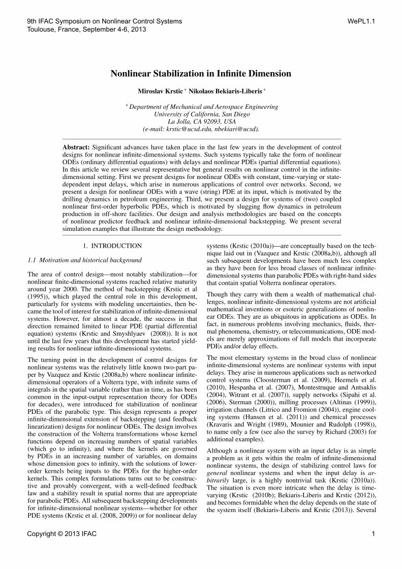
Fig. 1. A drillstring used in oil drilling. The angular displace-ment u of the drillstring is controlled through a torque U .

additional important results on the stabilization of nonlinearsystems with input and state delays have been developed byJankovic (2001, 2009), Karafyllis (2006, 2010), Karafyllisand Krstic (2012), Mazenc and Bliman (2006), Mazenc at al.(2004), Mazenc and Niculescu (2011).

Once the designer is equipped with the capability to overcomea delay at the input, i.e., the transport PDE process in theactuator line, there is every reason to ask whether other types ofinfinite-dimensional dynamics at the input can be compensated.This line of pursuit for infinite-dimensional dynamics in theactuator line of a linear ODE plant was pursued by Krstic(2009b) for diffusion-dominated (parabolic) actuator dynamicsand by Krstic (2009c) for wave PDE actuator dynamics. Severalextensions, all considering linear ODE plants preceded by PDEactuator dynamics, are presented by Bekiaris-Liberis and Krstic(2010), Bekiaris-Liberis and Krstic (2011b), Krstic (2009a),Ren et al. (2012), Susto and Krstic (2010), Tang and Xie(2011a,b). Extending those results from the case where theplant is a linear ODE to the case where the plant is a nonlinearODE has proved much more challenging than for the casewhere the actuator dynamics are of the delay (transport PDE)type. Until recently, that is, as we show in this article anddiscuss next.

A representative engineering application in which wave PDEactuator dynamics are cascaded with a nonlinear ODE is oildrilling. A common type of instability in oil drilling is theso-called stick-slip oscillations (Jansen (1993)). This type ofinstability (which is caused by a specific composition of theground material) results in torsional vibrations of the drillstring,which can in turn severely damage the drilling facilities (seeFig. 1 taken from Sagert et al. (2013)). The torsional dynamicsof an oil drillstring are modeled as a wave PDE (that describesthe dynamics of the angular displacement of the drillstring)coupled with a nonlinear ODE that describes the dynamicsof the bottom angular velocity of the drill bit (Saldivar et al.(2011)). A control approach for the bottom angular velocitybased on the linearization of its dynamics is presented inSagert et al. (2013). In this article we present a design forgeneral nonlinear ODE plants with a wave PDE as its actuatordynamics. This design solves the oil drilling problem (globally)as a special case.

Liquid

Gas

Pressure sensors Topside

Bottom

Actuator

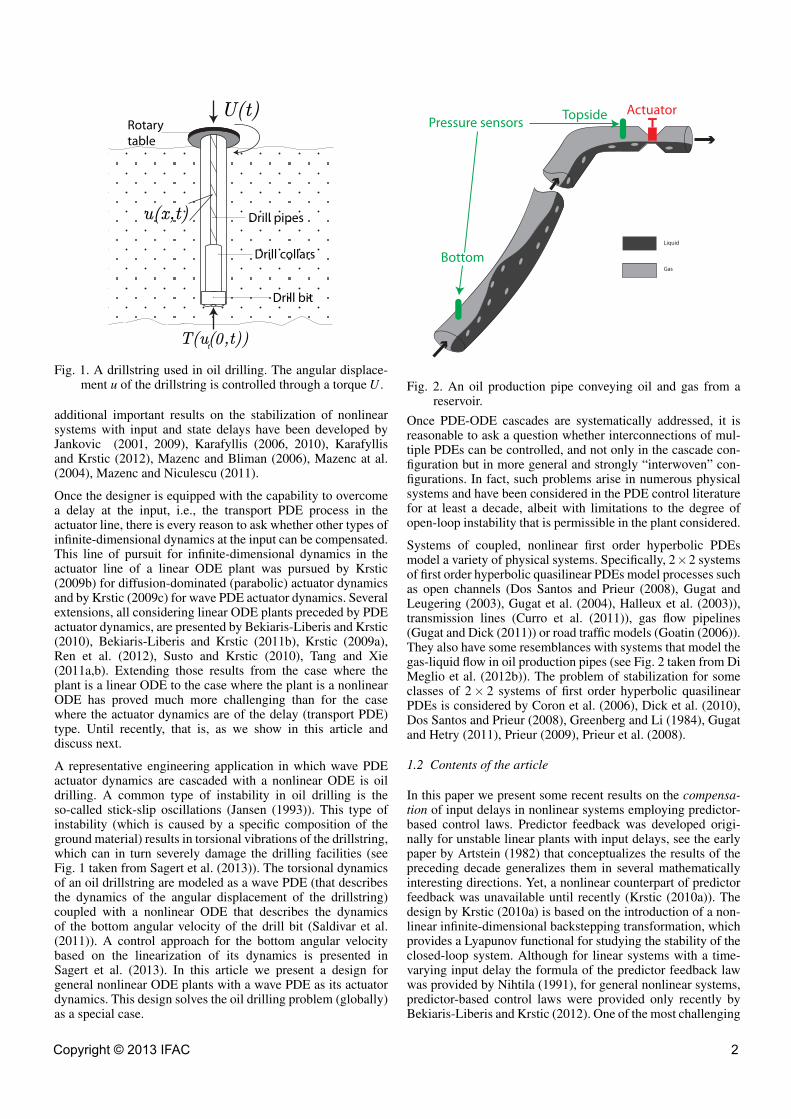
Fig. 2. An oil production pipe conveying oil and gas from areservoir.

Once PDE-ODE cascades are systematically addressed, it isreasonable to ask a question whether interconnections of mul-tiple PDEs can be controlled, and not only in the cascade con-figuration but in more general and strongly “interwoven” con-figurations. In fact, such problems arise in numerous physicalsystems and have been considered in the PDE control literaturefor at least a decade, albeit with limitations to the degree ofopen-loop instability that is permissible in the plant considered.

Systems of coupled, nonlinear first order hyperbolic PDEsmodel a variety of physical systems. Specifically, 2×2 systemsof first order hyperbolic quasilinear PDEs model processes suchas open channels (Dos Santos and Prieur (2008), Gugat andLeugering (2003), Gugat et al. (2004), Halleux et al. (2003)),transmission lines (Curro et al. (2011)), gas flow pipelines(Gugat and Dick (2011)) or road traffic models (Goatin (2006)).They also have some resemblances with systems that model thegas-liquid flow in oil production pipes (see Fig. 2 taken from DiMeglio et al. (2012b)). The problem of stabilization for someclasses of 2× 2 systems of first order hyperbolic quasilinearPDEs is considered by Coron et al. (2006), Dick et al. (2010),Dos Santos and Prieur (2008), Greenberg and Li (1984), Gugatand Hetry (2011), Prieur (2009), Prieur et al. (2008).

1.2 Contents of the article

In this paper we present some recent results on the compensa-tion of input delays in nonlinear systems employing predictor-based control laws. Predictor feedback was developed origi-nally for unstable linear plants with input delays, see the earlypaper by Artstein (1982) that conceptualizes the results of thepreceding decade generalizes them in several mathematicallyinteresting directions. Yet, a nonlinear counterpart of predictorfeedback was unavailable until recently (Krstic (2010a)). Thedesign by Krstic (2010a) is based on the introduction of a non-linear infinite-dimensional backstepping transformation, whichprovides a Lyapunov functional for studying the stability of theclosed-loop system. Although for linear systems with a time-varying input delay the formula of the predictor feedback lawwas provided by Nihtila (1991), for general nonlinear systems,predictor-based control laws were provided only recently byBekiaris-Liberis and Krstic (2012). One of the most challenging


problems in delay systems is the control of systems with state-dependent delays, as highlighted by Richard (2003). The firstsystematic approach for designing stabilizing controllers fornonlinear systems with state-dependent delays introduced byBekiaris-Liberis and Krstic (2013). The design is based on pre-dictor feedback. The key challenge that is resolved in Bekiaris-Liberis and Krstic (2013) is the definition of the predictor state:The state-dependence of the delay makes the prediction horizondependent on future values of the state which are unavailable.

We also consider finite-dimensional nonlinear plants which arecontrolled through a string and we design a predictor-basedfeedback law that compensates the string (wave) dynamicsin the input of the plant. Our design is based on a prelimi-nary transformation which allows one to convert the problemof the compensation of the wave PDE, to a problem of thecompensation of a 2× 2 system of first order transport equa-tions which convect in opposite directions (see, for example,Vazquez et al. (2011a)), for an augmented (by one integrator)plant. We then introduce the infinite-dimensional backsteppingtransformations for the two transport states, which transformthe new, augmented system to a target system. With the aid ofthe backstepping transformations we prove global asymptoticstability of the closed-loop system by constructing a Lyapunovfunctional.

Finally, we review some recent results on the local exponentialH2 stabilization of a 2× 2 system of first order hyperbolicquasilinear PDEs using backstepping developed by Coron et al.(2012) and Vazquez et al. (2011b). Specifically, we present thedesign of a control law that stabilizes the linearized system us-ing the recently developed backstepping technique of Vazquezet al. (2011a) for 2×2 systems of linear hyperbolic PDEs (seealso Di Meglio et al. (2012a) for an extension to n×n systems).We then prove the local exponential stability of the closed-loop system in the H2 norm by constructing a strict Lyapunovfunctional with the aid of the backstepping transformations.

1.3 Oganization

Section 2 is devoted to nonlinear systems with input delays.We introduce the predictor-based design for constant delaysin Section 2.1 For time-varying delays the predictor feedbackdesign is presented in Section 2.2. State-dependent delays aretreated in Section 2.3. In Section 3 we present a design thatcompensates the wave actuator dynamics in nonlinear systems.In Section 4 we are dealing with a 2 × 2 system of firstorder quasilinear PDEs for which we design a control law thatachieves local exponential stability.

2. NONLINEAR SYSTEMS WITH INPUT DELAYS

One of the main obstacles in designing globally stabilizingcontrol laws for nonlinear systems with long input delays is thefinite escape phenomenon. The input delay may be so large thatthe control signal can not reach the plant before its state escapesto infinity. Therefore, in the following we assume that the plantX = f (X ,ω) is forward complete, that is, for every initialcondition and every bounded input signal the correspondingsolution is defined for all t ≥ 0.

Our predictor-based designs are based on a (possibly time-varying) feedback law κ(t,X(t)), which is assumed to be pe-riodic in its first argument and locally Lipschitz, that globally

stabilizes the delay-free plant, i.e., X(t) = f (X(t),κ(t,X(t))) isglobally asymptotically stable.

2.1 Constant delay

In this section we focus on nonlinear systems with constantinput delay, i.e, systems of the form

X(t) = f (X(t),U(t−D)) . (1)

The predictor-based control law for plant (1) is

U(t) = κ(t +D,P(t)) (2)

P(t) = X(t)+∫ t

t−Df (P(θ),U(θ))dθ , (3)

where the initial condition for the integral equation for P(t) isdefined for all θ ∈ [t0−D, t0] (t0 is the initial time which mustbe given because the closed-loop system is time-varying) as

P(θ) = X(t0)+∫ θ

t0−Df (P(σ),U(σ))dσ . (4)

The signal P(t) represents the D time-units ahead predictorof X , i.e., P(t) = X(t + D). In the case of linear systemsthe predictor P(t) is given explicitly using the variation ofconstants formula, with the initial condition P(t −D) = X(t),as P(t) = eADX(t) +

∫ tt−D eA(t−θ)BU(θ)dθ . For systems that

are nonlinear, P(t) cannot be written explicitly, for the samereason as a nonlinear ODE cannot be solved explicitly. So werepresent P(t) implicitly using the nonlinear integral equation(3). The computation of P(t) from (3) is straightforward witha discretized implementation in which P(t) is assigned valuesbased on the right-hand side of (3), which involves earliervalues of P and the values of the input U .

Together with the predictor-based control law (2) we definethe infinite-dimensional backstepping transformation of theactuator state given by

W (t) =U(t)−κ(t +D,P(t)), (5)

together with its inverse

U(t) =W (t)+κ(t +D,Π(t)), (6)

where 1

Π(t)=X(t)+∫ t

t−Df (Π(θ),κ(θ+D,Π(θ))+W (θ))dθ , (7)

with initial condition for all θ ∈ [t0−D, t0]

Π(θ) = X(t0)

+∫ θ

t0−Df (Π(σ),κ(σ +D,Π(σ))+W (σ))dσ . (8)

The backstepping transformation maps the original system (1)into the “target system” given by

1 The quantities P in (3) and Π in (7) are identical. However, we use twodistinct symbols for the same quantity because, in one case, P is expressedin terms of X and U , for the direct backstepping transformation, while, in theother case, Π is expressed in terms of X and W , for the inverse backsteppingtransformation.


X(t) = f (X(t),κ(t,X(t))+W (t−D)) (9)

W (t) = 0, for t ≥ t0. (10)

We have the following result. Its proof can be found in Krstic(2010a).Theorem 1. Let X = f (X ,ω) be forward complete and X(t) =f (X(t),κ(t,X(t))) globally uniformly asymptotically stable.Consider the closed-loop system consisting of the plant (1) andthe control law (2), (3). There exists a class K L function βsuch that for all initial conditions X(t0) ∈ Rn, U(t0 + θ);θ ∈[−D,0] ∈ L∞[−D,0] the following holds

Ω(t)≤ β (Ω(t0), t− t0) (11)

Ω(t) = |X(t)|+ supt−D≤θ≤t

|U(θ)|, (12)

for all t ≥ t0 ≥ 0.

If the global asymptotic stability assumption in Theorem 1is strengthened with an input-to-state stability assumption ofthe plant X(t) = f (X(t),κ(t,X(t))+ω(t)) with respect to ω ,one can construct a Lyapunov functional 2 for the closed-loopsystem. Towards that end we observe from the “target system”(9), (10) that W (t−D) vanishes in finite time (in D time-units).Hence, under the input-to-state stability assumption on the plantX(t) = f (X(t),κ(t,X(t))+ω(t)) with respect to ω one canconstruct a Lyapunov functional for the system in the (X ,W )variables. Using Malisoff and Mazenc (2005) there exists a C1

function S : R+×Rn→R+ and class K∞ functions α1, α2, α3,α4 such that

α3 (|X(t)|)≤ S (t,X(t))≤ α4 (|X(t)|) (13)

S(t,X(t))≤−α1(|X(t)|)+α2(|W (t−D)|), (14)

S(t,X(t)) =∂S(t,X(t))

∂ t+

∂S(t,X(t))∂X

× f (X(t),κ(t,X(t))+W (t−D)) . (15)

The Lyapunov functional for the “target system” is then

V (t) = S (t,X(t))+2c

∫ L(t)

0

α2(r)r

dr, (16)

where α2(r)r is a class K function or α2 has been appropriately

majorized so this is true (with no generality loss), c > 0 isarbitrary and

L(t) = supt−D≤θ≤t

∣∣∣ec(θ−t+D)W (θ)∣∣∣ . (17)

Using the inverse backstepping transformation (6) one can thenprove stability in the original variables (X ,U). The functionalL can be also written directly in terms of the original variables(X ,U) as

L(t) = supt−D≤θ≤t

∣∣∣ec(θ−t+D) (U(θ)−κ(θ +D,P(θ)))∣∣∣ , (18)

where P is given in terms of (X ,U) from (3). The two differentrepresentations of the functional L, namely, representations(17) and (18), reveal one of the benefits of the backsteppingtransformation: If the construction of the functional L in terms2 The availability of a Lyapunov functional enables one in principle, to study,robustness of the predictor feedback to parametric uncertainties, its disturbanceattenuation properties, and the inverse-optimal re-design problem.

of the transformed actuator state W appears to be non-trivial,its form in terms of the original variables (X ,U), i.e., relation(18), is rather impossible to guess without the backstepping andpredictor transformations.

2.2 Time-varying delay

In this section we consider plants of the form

X(t) = f (X(t),U(t−D(t))) , (19)

where D is a positive-valued continuously differentiable func-tion of time. We define the functions

φ(t) = t−D(t) (20)

σ(t) = φ−1(t), (21)

and we refer to the quantity t−φ(t) = D(t) as the delay time.This is the time interval that indicates how long ago the controlsignal that is currently affects the plant was actually applied.The main goal of this section is to determine the predictor state,i.e., the quantity P such that X (σ(t)) = P(t). From now on werefer to the quantity σ(t)− t as the prediction horizon. Thisis the time interval which indicates after how long an inputsignal that is currently applied affects the plant. In the constantdelay case, the prediction horizon is equal to the delay time,i.e., t−φ(t) = D = σ(t)− t. The predictor-based control law is

U(t) = κ (σ(t),P(t)) (22)

P(t) = X(t)+∫ t

t−D(t)

f (P(θ),U(θ))dθφ ′ (φ−1(θ))

, (23)

with an initial condition for all θ ∈ [t0−D(t0), t0] as

P(θ) = X(t0)+∫ θ

t0−D(t0)

f (P(σ),U(σ))dσφ ′ (φ−1(σ))

. (24)

The fact that P(t) = X (σ(t)) can be established by applying thechange of variables t = σ(τ) in (19).

From (23) one can observe that the function dσ(θ)dθ = 1

φ ′(φ−1(θ))is employed in the control law. Therefore, one has to appropri-ately restrict the delay time D(t) such that φ ′(t) 6= 0 for all t ≥ 0.Actually, we impose the condition φ ′(t) > 0 for all t ≥ 0. Thereason is that if φ ′(t) > 0 for all t ≥ 0 then the control signalis able to reach the plant and it does not change the directionof propagation of the control signal (the plant keeps receivingcontrol inputs that are never older than the ones it has alreadyreceived). Besides the condition φ ′(t) > 0 for all t ≥ 0, whichcan be also expressed in terms of the delay function as D(t)< 1,for all t ≥ 0, we also assume that the delay can not disappearinstantaneously, i.e., φ ′ (or D) is bounded. Also, the delay hasto be positive (to guarantee the causality of the system) andbounded (such that the control signal eventually reaches theplant).

We are now ready to state the following theorem, the proof ofwhich can be found in Bekiaris-Liberis and Krstic (2012).Theorem 2. Let X = f (X ,ω) be forward complete and X(t) =f (X(t),κ(t,X(t))) globally uniformly asymptotically stable.Let the delay time D(t) = t − φ(t) be positive and uniformlybounded from above, and its rate D(t) be smaller than oneand uniformly bounded from below. Consider the closed-loopsystem consisting of the plant (19) and the control law (22),


delay x = f (x,u)

1

transport PDE (nonlinear)ODE

U X

1

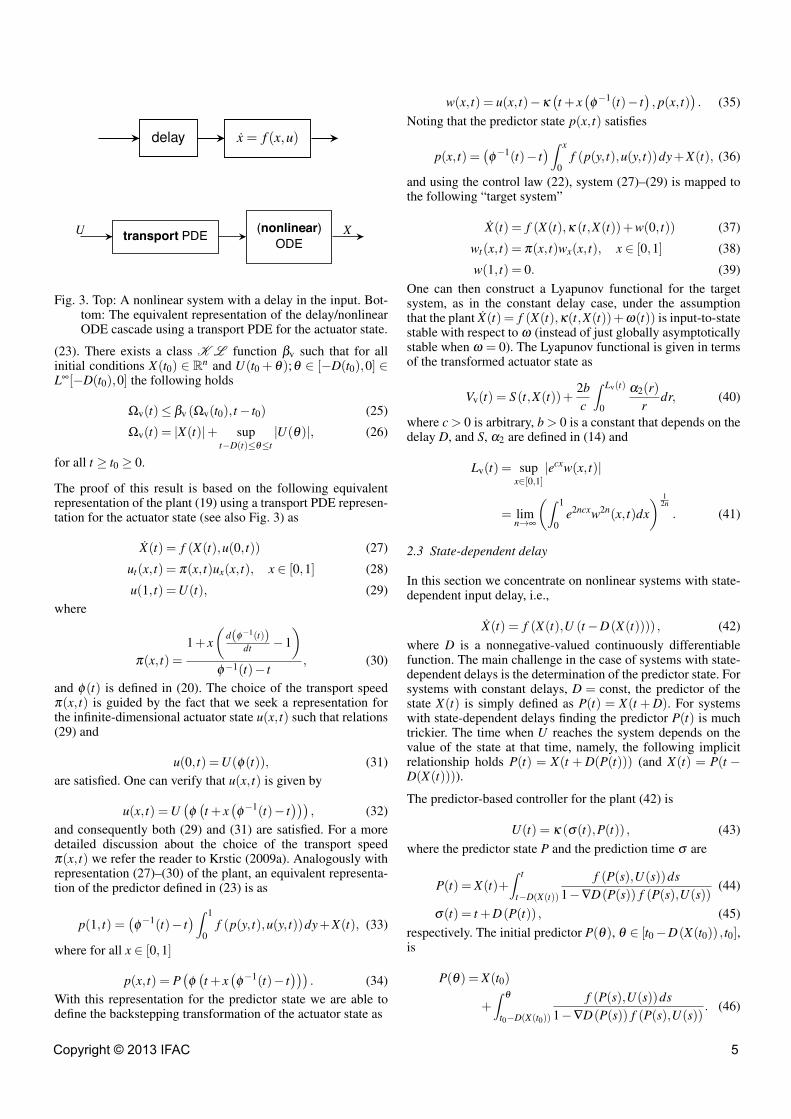
Fig. 3. Top: A nonlinear system with a delay in the input. Bot-tom: The equivalent representation of the delay/nonlinearODE cascade using a transport PDE for the actuator state.

(23). There exists a class K L function βv such that for allinitial conditions X(t0) ∈ Rn and U(t0 + θ);θ ∈ [−D(t0),0] ∈L∞[−D(t0),0] the following holds

Ωv(t)≤ βv (Ωv(t0), t− t0) (25)

Ωv(t) = |X(t)|+ supt−D(t)≤θ≤t

|U(θ)|, (26)

for all t ≥ t0 ≥ 0.

The proof of this result is based on the following equivalentrepresentation of the plant (19) using a transport PDE represen-tation for the actuator state (see also Fig. 3) as

X(t) = f (X(t),u(0, t)) (27)

ut(x, t) = π(x, t)ux(x, t), x ∈ [0,1] (28)

u(1, t) =U(t), (29)where

π(x, t) =1+ x

(d(φ−1(t))

dt −1)

φ−1(t)− t, (30)

and φ(t) is defined in (20). The choice of the transport speedπ(x, t) is guided by the fact that we seek a representation forthe infinite-dimensional actuator state u(x, t) such that relations(29) and

u(0, t) =U(φ(t)), (31)are satisfied. One can verify that u(x, t) is given by

u(x, t) =U(φ(t + x

(φ−1(t)− t

))), (32)

and consequently both (29) and (31) are satisfied. For a moredetailed discussion about the choice of the transport speedπ(x, t) we refer the reader to Krstic (2009a). Analogously withrepresentation (27)–(30) of the plant, an equivalent representa-tion of the predictor defined in (23) is as

p(1, t) =(φ−1(t)− t

)∫ 1

0f (p(y, t),u(y, t))dy+X(t), (33)

where for all x ∈ [0,1]

p(x, t) = P(φ(t + x

(φ−1(t)− t

))). (34)

With this representation for the predictor state we are able todefine the backstepping transformation of the actuator state as

w(x, t) = u(x, t)−κ(t + x

(φ−1(t)− t

), p(x, t)

). (35)

Noting that the predictor state p(x, t) satisfies

p(x, t) =(φ−1(t)− t

)∫ x

0f (p(y, t),u(y, t))dy+X(t), (36)

and using the control law (22), system (27)–(29) is mapped tothe following “target system”

X(t) = f (X(t),κ (t,X(t))+w(0, t)) (37)

wt(x, t) = π(x, t)wx(x, t), x ∈ [0,1] (38)

w(1, t) = 0. (39)One can then construct a Lyapunov functional for the targetsystem, as in the constant delay case, under the assumptionthat the plant X(t) = f (X(t),κ(t,X(t))+ω(t)) is input-to-statestable with respect to ω (instead of just globally asymptoticallystable when ω = 0). The Lyapunov functional is given in termsof the transformed actuator state as

Vv(t) = S (t,X(t))+2bc

∫ Lv(t)

0

α2(r)r

dr, (40)

where c > 0 is arbitrary, b > 0 is a constant that depends on thedelay D, and S, α2 are defined in (14) and

Lv(t) = supx∈[0,1]

|ecxw(x, t)|

= limn→∞

(∫ 1

0e2ncxw2n(x, t)dx

) 12n

. (41)

2.3 State-dependent delay

In this section we concentrate on nonlinear systems with state-dependent input delay, i.e.,

X(t) = f (X(t),U (t−D(X(t)))) , (42)where D is a nonnegative-valued continuously differentiablefunction. The main challenge in the case of systems with state-dependent delays is the determination of the predictor state. Forsystems with constant delays, D = const, the predictor of thestate X(t) is simply defined as P(t) = X(t +D). For systemswith state-dependent delays finding the predictor P(t) is muchtrickier. The time when U reaches the system depends on thevalue of the state at that time, namely, the following implicitrelationship holds P(t) = X(t + D(P(t))) (and X(t) = P(t −D(X(t)))).

The predictor-based controller for the plant (42) is

U(t) = κ (σ(t),P(t)) , (43)where the predictor state P and the prediction time σ are

P(t) = X(t)+∫ t

t−D(X(t))

f (P(s),U(s))ds1−∇D(P(s)) f (P(s),U(s))

(44)

σ(t) = t +D(P(t)) , (45)respectively. The initial predictor P(θ), θ ∈ [t0−D(X(t0)) , t0],is

P(θ) = X(t0)

+∫ θ

t0−D(X(t0))

f (P(s),U(s))ds1−∇D(P(s)) f (P(s),U(s))

. (46)


The fact that P(t) given in (44) is the σ(t)− t = D(P(t))time units ahead predictor of X(t), i.e., P(t) = X(σ(t)), can beestablished by performing a change of variables t = σ(τ) in theODE for X(t) given in (42) and noting from relations φ(t) = t−D(X(t)) and σ(t) = φ−1(t) that D(X(σ(t))) = σ(t)− t, whichimplies in particular that

dσ(t)dt

=1

1−∇D(P(t)) f (P(t),U(t)). (47)

As in the case of time-varying delays φ ′ and D must bepositive and bounded. The positiveness of φ ′ (or equivalentlyof σ ′) is guaranteed by imposing the following condition onthe solutions

Fc : ∇D(P(θ)) f (P(θ),U(θ))< c,

for all θ ≥ t0−D(X(t0)), (48)

for c ∈ (0,1]. We refer to F1 as the feasibility condition ofthe controller (43)–(45). Due to this condition, we obtain alocal result. Boundness of φ ′ and D is then guaranteed by theboundness of the system’s norm. We obtain the following result.Its proof can be found in Bekiaris-Liberis and Krstic (2013).Theorem 3. Let X = f (X ,ω) be forward complete and X(t) =f (X(t),κ(t,X(t))) globally uniformly asymptotically stable.Consider the closed-loop system consisting of the plant (42)and the control law (43)–(45). There exist a class K functionψRoA and a class K L function βs such that for all initialconditions X(t0) ∈ Rn such that U is locally Lipschitz on theinterval [t0−D(X(t0)), t0) and which satisfy

Ωs(t0)< ψRoA (c) , (49)

for some 0 < c < 1, where

Ωs(t) = |X(t)|+ supt−D(X(t))≤θ≤t

|U(θ)| , (50)

the following holds

Ωs(t)≤ βs (Ωs(t0), t− t0) , (51)

for all t ≥ t0 ≥ 0. Furthermore, there exists a class K functionδ ∗ such that, for all t ≥ t0 ≥ 0,

D(X(t))≤D(0)+δ ∗ (c) (52)∣∣D(X(t))∣∣≤ c. (53)

A Lyapunov functional for the closed-loop system consisting ofthe plant (42) and the control law (43)–(45) is

Vs(t) = S (t,X(t))+2g

∫ Ls(t)

0

α2 (r)r

dr, (54)

where g > 0 is arbitrary, S, α2 are defined in (14) and

Ls(t) = supt−D(X(t))≤θ≤t

∣∣∣eg(θ+D(P(θ))−t)W (θ)∣∣∣ (55)

W (θ) =U(θ)−κ (θ +D(P(θ)),P(θ)) , (56)

where P is given in terms of (X ,U) in (44).

The following example illustrates the fact that global stabiliza-tion is not possible even for linear systems.

0 0.1 0.2 0.3 0.4 0.5 0.6 0.70

0.1

0.2

0.3

0.4

0.5

0.6

0.7

0.8

0.9

t

x(t)

0 0.1 0.2 0.3 0.4 0.5 0.6 0.7−0.2

−0.1

0

0.1

0.2

0.3

0.4

0.5

0.6

0.7

φ(t)

t

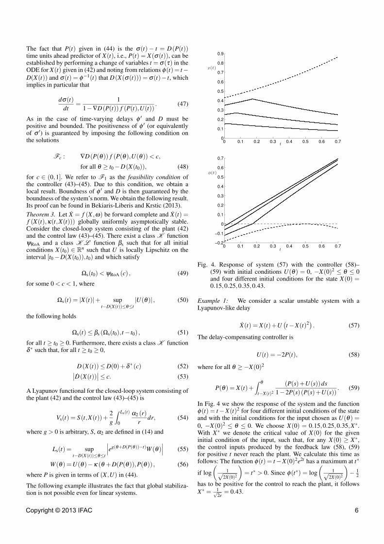
Fig. 4. Response of system (57) with the controller (58)–(59) with initial conditions U(θ) = 0, −X(0)2 ≤ θ ≤ 0and four different initial conditions for the state X(0) =0.15,0.25,0.35,0.43.

Example 1: We consider a scalar unstable system with aLyapunov-like delay

X(t) = X(t)+U(t−X(t)2) . (57)

The delay-compensating controller is

U(t) =−2P(t), (58)

where for all θ ≥−X(0)2

P(θ) = X(t)+∫ θ

t−X(t)2

(P(s)+U(s))ds1−2P(s)(P(s)+U(s))

. (59)

In Fig. 4 we show the response of the system and the functionφ(t) = t−X(t)2 for four different initial conditions of the stateand with the initial conditions for the input chosen as U(θ) =0, −X(0)2 ≤ θ ≤ 0. We choose X(0) = 0.15,0.25,0.35,X∗.With X∗ we denote the critical value of X(0) for the giveninitial condition of the input, such that, for any X(0) ≥ X∗,the control inputs produced by the feedback law (58), (59)for positive t never reach the plant. We calculate this time asfollows: The function φ(t) = t−X(0)2e2t has a maximum at t∗

if log(

1√2X(0)2

)= t∗ > 0. Since φ(t∗) = log

(1√

2X(0)2

)− 1

2

has to be positive for the control to reach the plant, it followsX∗ = 1√

2e= 0.43.


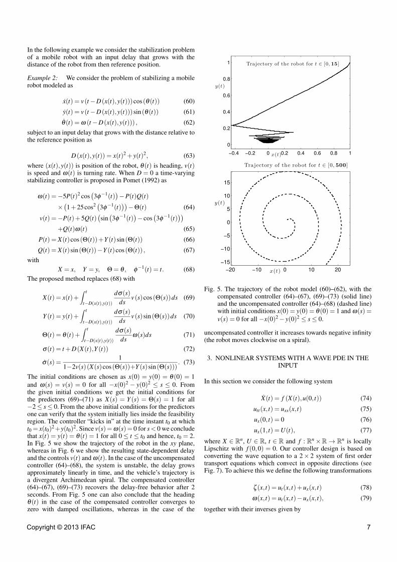
In the following example we consider the stabilization problemof a mobile robot with an input delay that grows with thedistance of the robot from then reference position.

Example 2: We consider the problem of stabilizing a mobilerobot modeled as

x(t) = v(t−D(x(t),y(t)))cos(θ(t)) (60)

y(t) = v(t−D(x(t),y(t)))sin(θ(t)) (61)

θ(t) = ω (t−D(x(t),y(t))) , (62)subject to an input delay that grows with the distance relative tothe reference position as

D(x(t),y(t)) = x(t)2 + y(t)2, (63)where (x(t),y(t)) is position of the robot, θ(t) is heading, v(t)is speed and ω(t) is turning rate. When D = 0 a time-varyingstabilizing controller is proposed in Pomet (1992) as

ω(t) =−5P(t)2 cos(3φ−1(t)

)−P(t)Q(t)

×(1+25cos2 (3φ−1(t)

))−Θ(t) (64)

v(t) =−P(t)+5Q(t)(sin(3φ−1(t)

)− cos

(3φ−1(t)

))+Q(t)ω(t) (65)

P(t) = X(t)cos(Θ(t))+Y (t)sin(Θ(t)) (66)

Q(t) = X(t)sin(Θ(t))−Y (t)cos(Θ(t)) , (67)with

X = x, Y = y, Θ = θ , φ−1(t) = t. (68)The proposed method replaces (68) with

X(t) = x(t)+∫ t

t−D(x(t),y(t))

dσ(s)ds

v(s)cos(Θ(s))ds (69)

Y (t) = y(t)+∫ t

t−D(x(t),y(t))

dσ(s)ds

v(s)sin(Θ(s))ds (70)

Θ(t) = θ(t)+∫ t

t−D(x(t),y(t))

dσ(s)ds

ω(s)ds (71)

σ(t) = t +D(X(t),Y (t)) (72)

σ(s) =1

1−2v(s)(X(s)cos(Θ(s))+Y (s)sin(Θ(s))). (73)

The initial conditions are chosen as x(0) = y(0) = θ(0) = 1and ω(s) = v(s) = 0 for all −x(0)2 − y(0)2 ≤ s ≤ 0. Fromthe given initial conditions we get the initial conditions forthe predictors (69)–(71) as X(s) = Y (s) = Θ(s) = 1 for all−2≤ s≤ 0. From the above initial conditions for the predictorsone can verify that the system initially lies inside the feasibilityregion. The controller “kicks in” at the time instant t0 at whicht0 = x(t0)2+y(t0)2. Since v(s)=ω(s)= 0 for s< 0 we concludethat x(t) = y(t) = θ(t) = 1 for all 0≤ t ≤ t0 and hence, t0 = 2.In Fig. 5 we show the trajectory of the robot in the xy plane,whereas in Fig. 6 we show the resulting state-dependent delayand the controls v(t) and ω(t). In the case of the uncompensatedcontroller (64)–(68), the system is unstable, the delay growsapproximately linearly in time, and the vehicle’s trajectory isa divergent Archimedean spiral. The compensated controller(64)–(67), (69)–(73) recovers the delay-free behavior after 2seconds. From Fig. 5 one can also conclude that the headingθ(t) in the case of the compensated controller converges tozero with damped oscillations, whereas in the case of the

−0.4 −0.2 0 0.2 0.4 0.6 0.8 1

0

0.2

0.4

0.6

0.8

1

x(t)

y(t)

Trajectory of the robot for t ∈ [0, 15]

−20 −10 0 10 20

−15

−10

−5

0

5

10

15

Trajectory of the robot for t ∈ [0, 500]

x(t)

y(t)

Fig. 5. The trajectory of the robot model (60)–(62), with thecompensated controller (64)–(67), (69)–(73) (solid line)and the uncompensated controller (64)–(68) (dashed line)with initial conditions x(0) = y(0) = θ(0) = 1 and ω(s) =v(s) = 0 for all −x(0)2− y(0)2 ≤ s≤ 0.

uncompensated controller it increases towards negative infinity(the robot moves clockwise on a spiral).

3. NONLINEAR SYSTEMS WITH A WAVE PDE IN THEINPUT

In this section we consider the following system

X(t) = f (X(t),u(0, t)) (74)

utt(x, t) = uxx(x, t) (75)

ux(0, t) = 0 (76)

ux(1, t) =U(t), (77)

where X ∈ Rn, U ∈ R, t ∈ R and f : Rn×R→ Rn is locallyLipschitz with f (0,0) = 0. Our controller design is based onconverting the wave equation to a 2× 2 system of first ordertransport equations which convect in opposite directions (seeFig. 7). To achieve this we define the following transformations

ζ (x, t) = ut(x, t)+ux(x, t) (78)

ω(x, t) = ut(x, t)−ux(x, t), (79)

together with their inverses given by


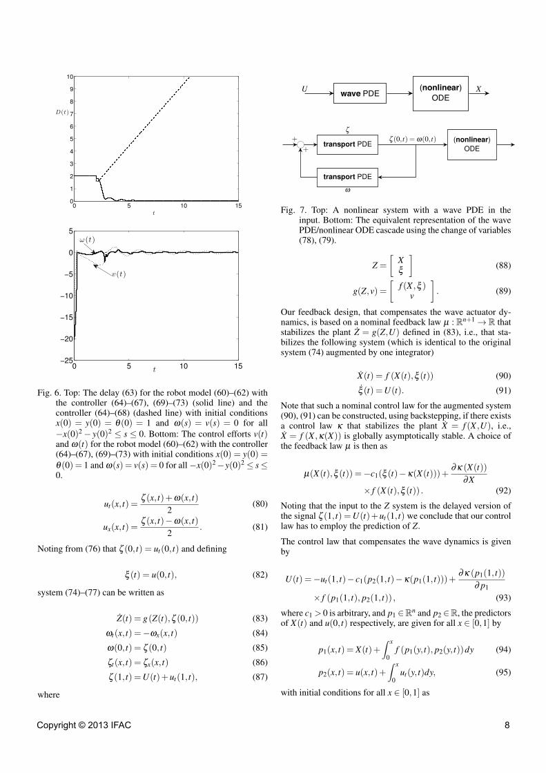
0 5 10 150

1

2

3

4

5

6

7

8

9

10

t

D(t)

0 5 10 15−25

−20

−15

−10

−5

0

5

t

v(t)

ω(t)

Fig. 6. Top: The delay (63) for the robot model (60)–(62) withthe controller (64)–(67), (69)–(73) (solid line) and thecontroller (64)–(68) (dashed line) with initial conditionsx(0) = y(0) = θ(0) = 1 and ω(s) = v(s) = 0 for all−x(0)2− y(0)2 ≤ s ≤ 0. Bottom: The control efforts v(t)and ω(t) for the robot model (60)–(62) with the controller(64)–(67), (69)–(73) with initial conditions x(0) = y(0) =θ(0) = 1 and ω(s) = v(s) = 0 for all−x(0)2−y(0)2 ≤ s≤0.

ut(x, t) =ζ (x, t)+ω(x, t)

2(80)

ux(x, t) =ζ (x, t)−ω(x, t)

2. (81)

Noting from (76) that ζ (0, t) = ut(0, t) and defining

ξ (t) = u(0, t), (82)

system (74)–(77) can be written as

Z(t) = g(Z(t),ζ (0, t)) (83)

ωt(x, t) =−ωx(x, t) (84)

ω(0, t) = ζ (0, t) (85)

ζt(x, t) = ζx(x, t) (86)

ζ (1, t) =U(t)+ut(1, t), (87)

where

wave PDE (nonlinear)ODE

U X

1

transport PDE

transport PDE

(nonlinear)ODE

ω

ζ+

+

ζ (0, t) = ω(0, t)

1

Fig. 7. Top: A nonlinear system with a wave PDE in theinput. Bottom: The equivalent representation of the wavePDE/nonlinear ODE cascade using the change of variables(78), (79).

Z =

[Xξ

](88)

g(Z,v) =[

f (X ,ξ )v

]. (89)

Our feedback design, that compensates the wave actuator dy-namics, is based on a nominal feedback law µ : Rn+1→ R thatstabilizes the plant Z = g(Z,U) defined in (83), i.e., that sta-bilizes the following system (which is identical to the originalsystem (74) augmented by one integrator)

X(t) = f (X(t),ξ (t)) (90)

ξ (t) =U(t). (91)

Note that such a nominal control law for the augmented system(90), (91) can be constructed, using backstepping, if there existsa control law κ that stabilizes the plant X = f (X ,U), i.e.,X = f (X ,κ(X)) is globally asymptotically stable. A choice ofthe feedback law µ is then as

µ(X(t),ξ (t)) =−c1(ξ (t)−κ(X(t)))+∂κ (X(t))

∂X× f (X(t),ξ (t)) . (92)

Noting that the input to the Z system is the delayed version ofthe signal ζ (1, t) =U(t)+ut(1, t) we conclude that our controllaw has to employ the prediction of Z.

The control law that compensates the wave dynamics is givenby

U(t) =−ut(1, t)− c1(p2(1, t)−κ(p1(1, t)))+∂κ (p1(1, t))

∂ p1

× f (p1(1, t), p2(1, t)) , (93)

where c1 > 0 is arbitrary, and p1 ∈Rn and p2 ∈R, the predictorsof X(t) and u(0, t) respectively, are given for all x ∈ [0,1] by

p1(x, t) = X(t)+∫ x

0f (p1(y, t), p2(y, t))dy (94)

p2(x, t) = u(x, t)+∫ x

0ut(y, t)dy, (95)

with initial conditions for all x ∈ [0,1] as


p1(x,0) = X(0)+∫ x

0f (p1(y,0), p2(y,0))dy (96)

p2(x,0) = u(x,0)+∫ x

0ut(y,0)dy. (97)

The name “predictors” for p1 and p2 is chosen to emphasizethat p1(1, t) and p2(1, t) are actually the 1-time units aheadpredictors of X(t) and u(0, t) respectively, i.e., it holds thatp1(1, t) = X(t+1) and p2(1, t) = u(0, t+1). This fact is shownin the next section 3 . Note that the control law (93) is directlyimplementable. To see this note that the predictors p1(1, t),p2(1, t) are computed, at each time t, based on the numericalintegration of the integrals in relation (94), (95) on the triangu-lar domain 0 ≤ y ≤ x, starting from the initial condition (in x)p1(0, t) = X(t), p2(0, t) = u(0, t).

Defining for any θ ∈ L∞[0,1] its supremum norm

supx∈[0,1]

|θ(x, t)|= ‖θ(t)‖∞, (98)

we are able to state the following result.Theorem 4. Consider the closed-loop system consisting of theplant (74)–(77) and the control law (93), (94), (95). Let theplant X = f (X ,v) be complete and the “disturbed” closed-loopsystem X = f (X ,µ(X)+ v) input-to-state stable and backwardcomplete. There exist a class K L function β such that

Ω(t)≤ β (Ω(0), t) (99)

Ω(t) = |X(t)|+‖u(t)‖∞ +‖ut(t)‖∞ +‖ux(t)‖∞, (100)for all t ≥ 0.

The proof of this result is based on the introduction of thefollowing invertible backstepping transformations of ω and ζdefined for all x ∈ [0,1] as

z(x, t) = ω(x, t)−µ(r(x, t)) (101)

w(x, t) = ζ (x, t)−µ(p(x, t)), (102)respectively, where for all x ∈ [0,1]

r(x, t) = Z(t)−∫ x

0g(r(y, t),ω(y, t))dy (103)

p(x, t) = Z(t)+∫ x

0g(p(y, t),ζ (y, t))dy, (104)

and µ is defined in (92). Transformation (101), (102) and thecontrol law (93)–(95) transform system (83)–(87) to the “targetsystem” given by

Z(t) = g(Z(t),µ(Z(t))+w(0, t)) (105)

zt(x, t) =−zx(x, t) (106)

z(0, t) = w(0, t) (107)

wt(x, t) = wx(x, t) (108)

w(1, t) = 0. (109)The stability of the “target system” can be then studied usingthe following Lyapunov functional3 Another way to see this is as follows. Construct first the standard 1-time unitahead predictor for Z satisfying (83) as P(t) = Z(t)+

∫ tt−1 g(P(θ),Ξ(θ))dθ ,

where Ξ(t + x− 1) = ζ (x, t). Defining P(t + x− 1) = p(x, t) we rewrite thepredictor as p(1, t)= Z(t)+

∫ 10 g(p(x, t),ζ (x, t))dx. Using definitions (88), (89)

and noting that p2(1, t) = u(0, t) +∫ 1

0 ux(x, t)dx +∫ 1

0 ut(x, t)dx, we get afterintegrating ux relations (94), (95) for x = 1.

V (t) = S(Z(t))+2c

∫ ‖v(t)‖c,∞0

α2(r)r

dr, (110)

where c > 0 is arbitrary, S and α2 are defined in (14) (note thatin the present case the closed-loop system is autonomous so Scan be chosen independent of t), and the new variable v(x, t),x ∈ [−1,1] is defined as

v(x, t) =

w(x, t), for all x ∈ [0,1]z∗(x, t), for all x ∈ [−1,0] , (111)

where ‖v(t)‖c,∞ = supx∈[−1,1] ec(1+x)|v(x, t)|, z∗(x, t) = z(−x, t).

3.1 Example

We consider the following system

X1(t) = X2(t)−X2(t)2u(0, t) (112)

X2(t) = u(0, t) (113)

utt(x, t) = uxx(x, t) (114)

ux(0, t) = 0 (115)

ux(1, t) =U(t). (116)System (112)–(113) is in the strict-feedforward form, andhence, is complete with respect to the input u(0, t). The nominalcontrol law (i.e., in the case where u(0, t)≡U(t))

U(t) =−X1(t)−2X2(t)−13

X2(t)3, (117)

renders the closed-loop system input-to-state stable and back-ward complete 4 . The control design that compensates the wavedynamics is

U(t) =−ut(1, t)−2(p3(1, t)+ p1(1, t)+2p2(1, t))

−23

p2(1, t)3− p2(1, t)+ p2(1, t)2 p3(1, t)

−(2+ p2(1, t)2) p3(1, t), (118)

where

p1(1, t) = X1(t)+X2(t)+∫ 1

0(1− x)u(x, t)dx

+∫ 1

0(1− x)2ut(x, t)dx

−∫ 1

0dx(

u(x, t)+∫ x

0ut(y, t)dy

)×(

X2(t)+∫ x

0(u(y, t)+(1− y)ut(y, t))dy

)2

(119)

p2(1, t) = X2(t)+∫ 1

0u(x, t)dx+

∫ 1

0(1− x)ut(x, t)dx (120)

p3(1, t) = u(1, t)+∫ 1

0ut(x, t)dx. (121)

We choose the initial conditions for the system as X1(0) = 1,X2(0) = 0 and the initial conditions for the actuator state asu(x,0) = ut(x,0) = 1, for all x ∈ [0,1]. In Fig. 8 we show the4 This fact follows from the fact that the control law (117) can be written asU = −φ1− φ2, where φ is the linearizing diffeomorphic transformation φ1 =X1 +X2 +

13 X3

2 , φ2 = X2, which transforms system (112)–(113) to φ1 = φ2 +U ,φ2 =U (see Krstic (2004)) .


0 1 2 3 4 5 6 7

−1

0

1

2

3

4

5

t

X1(t

)

0 1 2 3 4 5 6 7

−1.5

−1

−0.5

0

0.5

1

1.5

2

2.5

t

X2(t

)

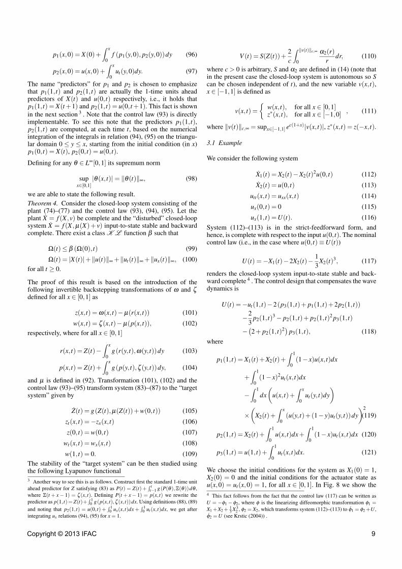
Fig. 8. The response of the states of the plant (112)–(113)with the control law (118)–(121) (solid line) and withthe nominal control law (117) (dashed line) for initialconditions as X1(0) = 1, X2(0) = 0 and u(x,0) = ut(x,0) =1, for all x ∈ [0,1].

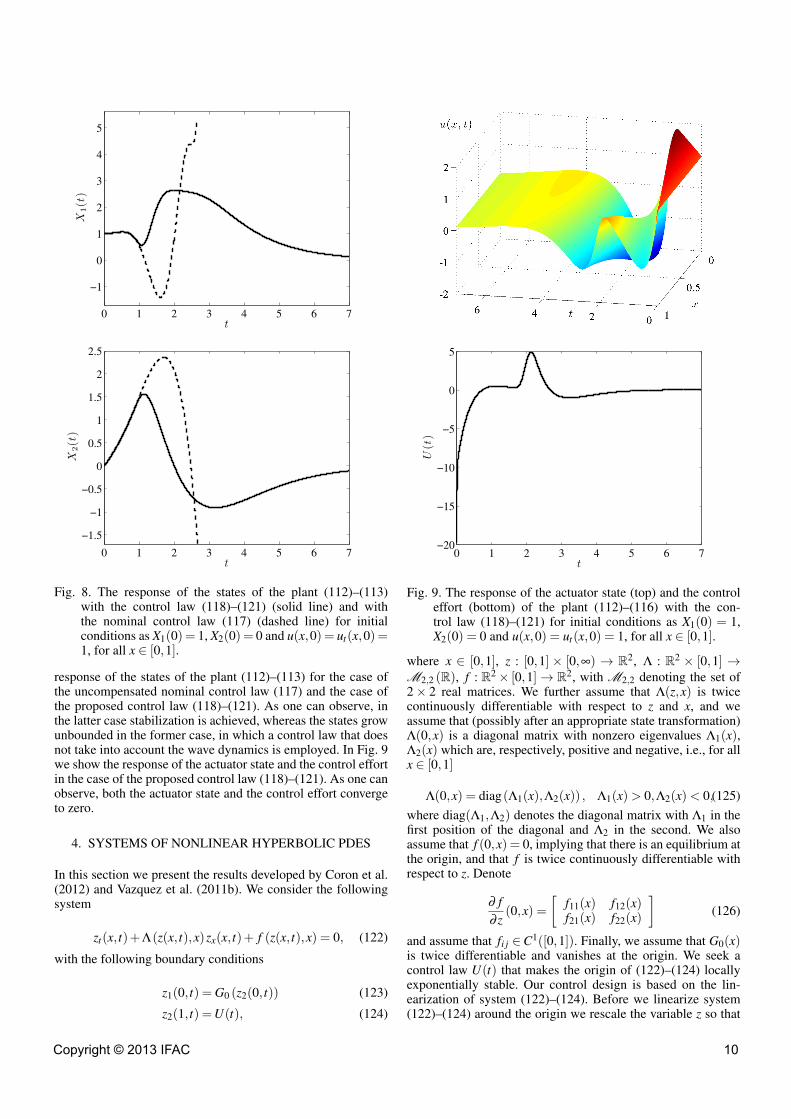
response of the states of the plant (112)–(113) for the case ofthe uncompensated nominal control law (117) and the case ofthe proposed control law (118)–(121). As one can observe, inthe latter case stabilization is achieved, whereas the states growunbounded in the former case, in which a control law that doesnot take into account the wave dynamics is employed. In Fig. 9we show the response of the actuator state and the control effortin the case of the proposed control law (118)–(121). As one canobserve, both the actuator state and the control effort convergeto zero.

4. SYSTEMS OF NONLINEAR HYPERBOLIC PDES

In this section we present the results developed by Coron et al.(2012) and Vazquez et al. (2011b). We consider the followingsystem

zt(x, t)+Λ(z(x, t),x)zx(x, t)+ f (z(x, t),x) = 0, (122)

with the following boundary conditions

z1(0, t) = G0 (z2(0, t)) (123)

z2(1, t) =U(t), (124)

0 1 2 3 4 5 6 7−20

−15

−10

−5

0

5

t

U(t

)

Fig. 9. The response of the actuator state (top) and the controleffort (bottom) of the plant (112)–(116) with the con-trol law (118)–(121) for initial conditions as X1(0) = 1,X2(0) = 0 and u(x,0) = ut(x,0) = 1, for all x ∈ [0,1].

where x ∈ [0,1], z : [0,1]× [0,∞) → R2, Λ : R2 × [0,1] →M2,2 (R), f : R2× [0,1]→ R2, with M2,2 denoting the set of2× 2 real matrices. We further assume that Λ(z,x) is twicecontinuously differentiable with respect to z and x, and weassume that (possibly after an appropriate state transformation)Λ(0,x) is a diagonal matrix with nonzero eigenvalues Λ1(x),Λ2(x) which are, respectively, positive and negative, i.e., for allx ∈ [0,1]

Λ(0,x) = diag(Λ1(x),Λ2(x)) , Λ1(x)> 0,Λ2(x)< 0,(125)where diag(Λ1,Λ2) denotes the diagonal matrix with Λ1 in thefirst position of the diagonal and Λ2 in the second. We alsoassume that f (0,x) = 0, implying that there is an equilibrium atthe origin, and that f is twice continuously differentiable withrespect to z. Denote

∂ f∂ z

(0,x) =[

f11(x) f12(x)f21(x) f22(x)

](126)

and assume that fi j ∈C1([0,1]). Finally, we assume that G0(x)is twice differentiable and vanishes at the origin. We seek acontrol law U(t) that makes the origin of (122)–(124) locallyexponentially stable. Our control design is based on the lin-earization of system (122)–(124). Before we linearize system(122)–(124) around the origin we rescale the variable z so that


we make the linear part of f antidiagonal since we present ourlinear design for the case of an antidiagonal linear f (with nogenerality loss). Defining the new variable w as

w = Φ(x)z (127)

Φ(x) = diag(φ1(x),φ2(x)) , (128)where

φ1(x) = e∫ x

0f11(y)Λ1(y)

dy(129)

φ2(x) = e−∫ x

0f22(y)Λ2(y)

dy, (130)

we rewrite system (122)–(124) in the new variables as (see Fig.10)

wt(x, t)−Σ(x)wx(x, t)−C(x)w(x, t)

+ΛNL(w(x, t),x)wx(x, t)+ fNL(w(x, t),x) = 0, (131)with boundary conditions as

w1(0, t) = qw2(0, t)+GNL (w2(0, t)) (132)

w2(1, t) =V (t), (133)where

Σ(x) =−Λ(0,x) (134)

C(x) =[

0 − f12(x)− f21(x) 0

](135)

V (t) = φ2(1)U(t) (136)

q =dG0(0)

dz, (137)

and the nonlinear perturbation terms ΛNL and fNL are such thatΛNL(0,x) = 0, fNL(0,x) =

∂ fNL∂w (0,x) = 0, GNL(0) = 0.

Our design is based on a backstepping design for the linear partof system (131). Defining w = [ u v ]

T , Λ1 = ε1, Λ2 = −ε2,f12 = −c1 and f21 = −c2 we rewrite the linear part of system(131) as

ut(x, t) =−ε1(x)ux(x, t)+ c1(x)v(x, t) (138)

vt(x, t) = ε2(x)vx(x, t)+ c2(x)u(x, t) (139)

u(0, t) = qv(0, t) (140)

v(1, t) =V (t). (141)System (138)–(141) is mapped to the following “target system”

αt(x, t) =−ε1(x)αx(x, t) (142)

βt(x, t) = ε2(x)βx(x, t) (143)

α(0, t) = qβ (0, t) (144)

β (1, t) = 0, (145)using the invertible backstepping transformation

α(x, t) = u(x, t)−∫ x

0Kuu(x,ξ )u(ξ , t)dξ

−∫ x

0Kuv(x,ξ )v(ξ , t)dyξ (146)

β (x, t) = v(x, t)−∫ x

0Kvu(x,ξ )u(ξ , t)dξ

−∫ x

0Kvv(x,ξ )v(ξ , t)dξ , (147)

and the control law

V (t) =∫ 1

0Kvu(1,x)u(x, t)dx+

∫ 1

0Kvv(1,x)v(x, t)dx.(148)

The kernels of the backstepping transformation satisfy the fol-lowing 2×2 system of linear hyperbolic PDEs on the triangulardomain T = (x,ξ ) : 0≤ ξ ≤ x≤ 1 which can be shown tobe well-posed (Vazquez et al. (2011a))

ε1(x)Kuux + ε1(ξ )Kuu

ξ =−ε ′1(ξ )Kuu− c2(ξ )Kuv (149)

ε1(x)Kuvx − ε2(ξ )Kuv

ξ = ε ′2(ξ )Kuv− c1(ξ )Kuu (150)

ε2(x)Kvux − ε1(ξ )Kvu

ξ = ε ′1(ξ )Kvu + c2(ξ )Kvv (151)

ε2(x)Kvvx + ε2(ξ )Kvv

ξ =−ε ′2(ξ )Kvv + c2(ξ )Kvu, (152)

with boundary conditions

Kuu(x,0) =ε2(0)

qε1(0)Kuv(x,0) (153)

Kuv(x,x) =c1(x)

ε1(x)+ ε2(x)(154)

Kvu(x,x) =− c2(x)ε1(x)+ ε2(x)

(155)

Kvv(x,0) =ε1(0)

qε2(0)Kvu(x,0). (156)

Using definition (127) and (136), the control law for the originalnonlinear system (122)–(124) is

U(t) =1

φ2(1)

∫ 1

0Kvu(1,x)φ1(x)z1(x, t)dx

+1

φ2(1)

∫ 1

0Kvv(1,x)φ2(x)z2(x, t)dx. (157)

With the control law (157) the boundary condition (124) for theclosed-loop system is written as

z1(1, t) =1

φ2(1)

∫ 1

0Kvu(1,x)φ1(x)z1(x, t)dx

+1

φ2(1)

∫ 1

0Kvv(1,x)φ2(x)z2(x, t)dx. (158)

Defining the H2 norm of z = [ z1 z2 ]T as

‖z(t)‖H2 =∫ 1

0z(x, t)T z(x, t)dx+

∫ 1

0zx(x, t)T zx(x, t)dx

+∫ 1

0zxx(x, t)T zxx(x, t)dx, (159)

and imposing the following compatibility conditions


0 = z1(0,0)−G0(z2(0,0)) (160)

0 = z2(1,0)−1

φ2(1)

∫ 1

0Kvu(1,x)φ1(x)z1(x,0)dx

− 1φ2(1)

∫ 1

0Kvv(1,x)φ2(x)z2(x,0)dx (161)

0 =−Λ1 (z(0,0),0)z1,x(0,0)− f1(z(0,0),0)+G′0(z2(0,0))

×(Λ2(z(0,0),0)z2,x(0,0)+ f2(z(0,0),0)) (162)

0 =∫ 1

0

Kvu(1,x)φ1(x)φ2(1)

Λ1 (z(x,0),x)z1,x(x,0)dx

+∫ 1

0

Kvu(1,x)φ1(x)φ2(1)

f1 (z(x,0),x)dx+∫ 1

0

Kvv(1,x)φ2(x)φ2(1)

×(Λ2 (z(x,0),x)z2,x(x,0)+ f2 (z(x,0),x))dx

−Λ2(z(1,0),1)z2,x(1,0)− f2(z(1,0),1), (163)we obtain the following result.Theorem 5. Consider the closed-loop system (122), (123),(158). Under the assumptions that Λ∈C2

(R2× [0,1]

), f (·,x)∈

C2(R2), ∂ f (0,·)

∂ z ∈ C1 ([0,1]), G0 ∈ C2 (R), for all initial con-dition z0 ∈ H2([0,1]) that satisfy the compatibility conditions(161)–(163), there exist δ > 0, λ > 0 and c > 0 such that if‖z(0)‖H2 < δ , then for all t ≥ 0

‖z(t)‖H2 ≤ ce−λ t‖z(0)‖H2 . (164)

Note that the compatibility conditions (161) and (163) dependon our feedback laws and therefore are not natural. They canbe omitted by considering a dynamical extension (see Coron etal. (2012)). The proof of Theorem 5 is based on employing thelinear backstepping transformation (146), (147) on the rescalednonlinear system (131), which results in the following targetsystem

γt −Σ(x)γx +F3 [γ,γx]+F4 [γ] = 0, (165)

where γ = [ α β ]T and F3, F4 are nonlinear functionals of

γ and γx (see Coron et al. (2012) for details). The H2 localexponential stability of the target system can be then studiedwith the following Lyapunov functional

S(t) =U(t)+V (t)+W (t) (166)

U(t) =∫ 1

0γT (x, t)D(x)γ(x, t)dx (167)

V (t) =∫ 1

0γT

t (x, t)R[γ](x)γt(x, t)dx (168)

W (t) =∫ 1

0γT

tt (x, t)R[γ](x)γtt(x, t)dx, (169)

where D(x) = diag(D1(x),D2(x)) is positive definite for allx ∈ [0,1] and R[γ] is a symmetric and positive definite matrixfor all supx∈[0,1] |γ(x, t)|< δ .

5. CONCLUSIONS

In our development we assume that the nonlinear plant underconsideration is forward complete and globally stabilizable.However, our predictor-based design can be applied to systemsthat are not forward complete (but they are globally stabilizablein the absence of the input delay) Krstic (2008) and to systemsthat are only locally stabilizable Bekiaris-Liberis and Krstic

transport PDE

transport PDE

G0(·)

U

z1

z2

z2(0, t)

z1(0, t)

1

transport PDE G0(·) transport PDEU

1

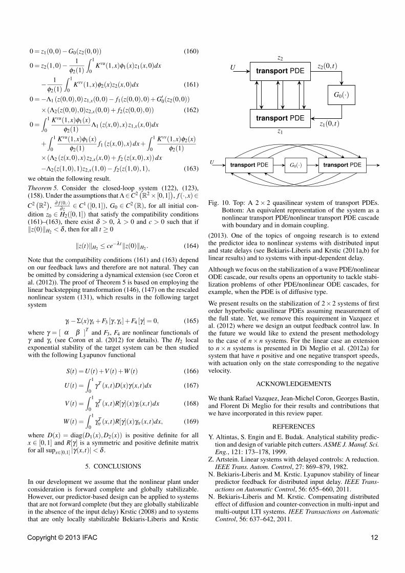
Fig. 10. Top: A 2× 2 quasilinear system of transport PDEs.Bottom: An equivalent representation of the system as anonlinear transport PDE/nonlinear transport PDE cascadewith boundary and in domain coupling.

(2013). One of the topics of ongoing research is to extendthe predictor idea to nonlinear systems with distributed inputand state delays (see Bekiaris-Liberis and Krstic (2011a,b) forlinear results) and to systems with input-dependent delay.

Although we focus on the stabilization of a wave PDE/nonlinearODE cascade, our results opens an opportunity to tackle stabi-lization problems of other PDE/nonlinear ODE cascades, forexample, when the PDE is of diffusive type.

We present results on the stabilization of 2×2 systems of firstorder hyperbolic quasilinear PDEs assuming measurement ofthe full state. Yet, we remove this requirement in Vazquez etal. (2012) where we design an output feedback control law. Inthe future we would like to extend the present methodologyto the case of n× n systems. For the linear case an extensionto n× n systems is presented in Di Meglio et al. (2012a) forsystem that have n positive and one negative transport speeds,with actuation only on the state corresponding to the negativevelocity.

ACKNOWLEDGEMENTS

We thank Rafael Vazquez, Jean-Michel Coron, Georges Bastin,and Florent Di Meglio for their results and contributions thatwe have incorporated in this review paper.

REFERENCES

Y. Altintas, S. Engin and E. Budak. Analytical stability predic-tion and design of variable pitch cutters. ASME J. Manuf. Sci.Eng., 121: 173–178, 1999.

Z. Artstein. Linear systems with delayed controls: A reduction.IEEE Trans. Autom. Control, 27: 869–879, 1982.

N. Bekiaris-Liberis and M. Krstic. Lyapunov stability of linearpredictor feedback for distributed input delay. IEEE Trans-actions on Automatic Control, 56: 655–660, 2011.

N. Bekiaris-Liberis and M. Krstic. Compensating distributedeffect of diffusion and counter-convection in multi-input andmulti-output LTI systems. IEEE Transactions on AutomaticControl, 56: 637–642, 2011.


N. Bekiaris-Liberis and M. Krstic. Compensating the dis-tributed effect of a wave PDE in the actuation or sensing pathof MIMO LTI Systems. Systems & Control Letters, 59: 713–719, 2010.

N. Bekiaris-Liberis and M. Krstic. Compensation of state-dependent input delay for nonlinear systems. IEEE Trans-actions on Automatic Control, to appear, 2013.

N. Bekiaris-Liberis and M. Krstic. Compensation of time-varying input and state delays for nonlinear systems. Journalof Dynamic Systems, Measurement, and Control, 134, paper011009, 2012.

M. B. G. Cloosterman, N. van de Wouw, W. P. M. H. Heemels,and H. Nijmeijer. Stability of networked control systemswith uncertain time-varying delays. IEEE Transactions onAutomatic Control, 54: 1575–1580, 2009.

J.-M. Coron, B. dAndrea-Novel, and G. Bastin. A strict Lya-punov function for boundary control of hyperbolic systemsof conservation laws. IEEE Trans. on Automatic Control, 52:2–11, 2006.

J.-M. Coron, R. Vazquez, M. Krstic, and G. Bastin. Localexponential H2 stabilization of a 2×2 quasilinear hyperbolicsystem using backstepping, submitted for publication, 2012.Available at: http://arxiv.org/abs/1208.6475.

C. Curro, D. Fusco and N. Manganaro. A reduction proce-dure for generalized Riemann problems with application tononlinear transmission lines. J. Phys. A: Math. Theor., 44:335205, 2011.

M. Dick, M. Gugat, and G. Leugering. Classical solutions andfeedback stabilisation for the gas flow in a sequence of pipes.Networks and heterogeneous media, 5: 691–709, 2010.

F. Di Meglio, R. Vazquez, and M. Krstic. Stabilization of alinear hyperbolic system with one boundary controlled trans-port PDE coupled with n counterconvecting PDEs. Proceed-ings of the IEEE Conference on Decision and Control, 2012.

F. Di Meglio, M. Krstic, R. Vazquez, N. Petit. Backsteppingstabilization of an underactuated 3 × 3 linear hyperbolicsystem of fluid flow transport equations. American ControlConference, 2012.

V. Dos Santos and C. Prieur. Boundary control of open channelswith numerical and experimental validations. IEEE Trans.Control Syst. Tech., 16: 1252–1264, 2008.

P. Goatin. The Aw-Rascle vehicular traffic flow model withphase transitions. Math. Comput. Modeling, 44: 287–303,2006.

J.-M. Greenberg and T.-T. Li. The effect of boundary dampingfor the quasilinear wave equations. Journal of DifferentialEquations, 52: 66–75, 1984.

M. Gugat and M. Dick. Time-delayed boundary feedback sta-bilization of the isothermal Euler equations with friction.Mathematical Control and Related Fields, 1: 469–491, 2011.

M. Gugat and M. Herty. Existence of classical solutions andfeedback stabilization for the flow in gas networks. ESAIMControl Optimization and Calculus of Variations, 17: 28–51,2011.

M. Gugat and G. Leugering. Global boundary controllability ofthe de St. Venant equations between steady states. Ann. Inst.H. Poincar Anal. Non Linaire, 20: 1–11, 2003.

M. Gugat, G. Leugering and E. Schmidt. Global controllabil-ity between steady supercritical flows in channel networks.Math. Methods Appl. Sci. 27: 781–802, 2004.

J. de Halleux, C. Prieur, J.-M. Coron, B. dAndra-Novel andG. Bastin. Boundary feedback control in networks of openchannels. Automatica, 39: 13651376, 2003.

M. Hansen, J. Stoustrup, J.-D. Bendtsen. Modeling of nonlinearmarine cooling systems with closed circuit flow. Proceedingsof the 18th IFAC World Congress, Milan, 2011.

W. P. M. H. Heemels, A. R. Teel, N. van de Wouw, D. Nesic.Networked control systems with communication constraints:tradeoffs between transmission intervals, delays and perfor-mance. IEEE Transactions on Automatic Control, 55: 1781–1796, 2010.

J. P. Hespanha, P. Naghshtabrizi and Y. Xu. A survey of recentresults in networked control systems. Proceedings of theIEEE, 95: 138–162, 2007.

M. Jankovic, “Control Lyapunov-Razumikhin functions and ro-bust stabilization of time delay systems,” IEEE Transactionson Automatic Control, vol. 46, pp. 1048–1060, 2001.

M. Jankovic, “Cross-Term Forwarding for Systems With TimeDelay,” IEEE Trans. Aut. Cont., vol. 54, pp. 498–511, 2009.

J. D. Jansen. Nonlinear dynamics of oilwell drillstrings. PhDthesis, Delft University of Technology, 1993.

I. Karafyllis. Finite-time global stabilization by means of time-varying distributed delay feedback. SIAM J. Control Optim.,45: 320–342, 2006.

I. Karafyllis. Stabilization by means of approximate predictorsfor systems with delayed input. SIAM Journal on Control andOptimization, 49: 1100–1123, 2011.

I. Karafyllis and M. Krstic. Nonlinear stabilization under sam-pled and delayed measurements, and with inputs subject todelay and zero-order hold. IEEE Transactions on AutomaticControl, 57: 1141–1154, 2012.

C. Kravaris and R. A. Wright, “Deadtime compensation fornonlinear processes,” AIChE J., 35: 1535–1542, 1989.

M. Krstic, I. Kanellakopoulos, and P. V. Kokotovic, Nonlinearand Adaptive Control Design, Wiley, 1995.

M. Krstic. Feedback linearizability and explicit integrator for-warding controllers for classes of feedforward systems. IEEETransactions on Automatic Control, 49: 1668–1682, 2004.

M. Krstic. On compensating long actuator delays in nonlinearcontrol. IEEE Trans. Autom. Control, 53: 1684–1688, 2008.

M. Krstic, Delay Compensation for Nonlinear, Adaptive, andPDE Systems, Birkhauser, 2009.

M. Krstic, “Compensating actuator and sensor dynamics gov-erned by diffusion PDEs,” Systems and Control Letters, vol.58, pp. 372–377, 2009.

M. Krstic, “Compensating a string PDE in the actuation orsensing path of an unstable ODE,” IEEE Transactions onAutomatic Control, vol. 54, pp. 1362–1368, 2009.

M. Krstic. Input delay compensation for forward completeand feedforward nonlinear systems. IEEE Transactions onAutomatic Control, 55: 287–303, 2010.

M. Krstic, “Lyapunov stability of linear predictor feedback fortime-varying input delay,” IEEE Trans. Autom. Control, vol.55, pp. 554–559, 2010.

M. Krstic, L. Magnis, and R. Vazquez. Nonlinear stabilizationof shock-like unstable equilibria in the viscous Burgers PDE.IEEE Transactions on Automatic Control, 53: 1678–1683,2008.

M. Krstic, L. Magnis, and R. Vazquez. Nonlinear control of theviscous Burgers equation: Trajectory generation, tracking,and observer design. Journal of Dynamic Systems, Measure-ment, and Control, 131: paper 021012 (8 pages), 2009.

M. Krstic and A. Smyshlyaev, Boundary Control of PDEs: ACourse on Backstepping Designs, SIAM, 2008.

X. Litrico and V. Fromion. Analytical approximation of open-channel flow for controller design. Applied Mathematical


Modelling, 28: 677–695, 2004.F. Mazenc and P.-A. Bliman. Backstepping design for time-

delay nonlinear systems. IEEE Trans. Autom. Control, 51:149–154, 2006.

M. Malisoff and F. Mazenc. Further remarks on strict input-to-state stable Lyapunov functions for time-varying systems.Automatica, 41: 1973–1978, 2005.

F. Mazenc, S. Mondie, and R. Francisco. Global asymptoticstabilization of feedforward systems with delay at the input.IEEE Trans. Autom. Control, 49: 844–850, 2004.

F. Mazenc and S.-I. Niculescu. Generating positive and stablesolutions through delayed state feedback. Automatica, 47:525–533, 2011.

L. A. Montestruque, P. Antsaklis. Stability of model-basednetworked control systems with time-varying transmissionlines. IEEE Trans. Autom. Control, 49: 1562–1572, 2004.

H. Mounier and J. Rudolph. Flatness-based control of nonlineardelay systems: A chemical reactor example. Int. J. Control,71: 871–890, 1998.

M. Nihtila. Finite pole assignment for systems with time-varying input delays. Proceedings of the IEEE Conferenceon Decision and Control, 1991.

J.-B. Pomet. Explicit design of time-varying stabilizing controllaws for a class of controllable systems without drift. Systems& Control Letters, 18: 147–158, 1992.

C. Prieur. Control of systems of conservation laws with bound-ary errors. Networks and Heterogeneous Media, 4: 393–407,2009.

C. Prieur, J. Winkin, and G. Bastin. Robust boundary controlof systems of conservation laws. Mathematics of Control,Signals, and Systems, 20: 173–197, 2008.

B. Ren, J.-M. Wang, and M. Krstic. Stabilization of an ODE-Schrodinger cascade. submitted for publication, 2012.

J-P. Richard. Time-delay systems: an overview of some recentadvances and open problems. Automatica, 39: 1667–1694,2003.

C. Sagert, F. Di Meglio, M. Krstic, P. Rouchon. Backsteppingand flatness approaches for stabilization of the stick-slip phe-nomenon for drilling. IFAC Symposium on System Structureand Control, 2013.

M. B. Saldivar, S. Mondie, J.-J. Loiseau, and V. Rasvan. Stick-Slip oscillations in oillwell drillstrings: Distributed Parame-ter and neutral type retarded model approaches. Proceedingsof the 18th IFAC World Congress, 2011.

R. Sipahi, S. Lammer, S.-I. Niculescu, D. Helbing. On stabilityanalysis and parametric design of supply networks under thepresence of transportation delays. Proceedings of the ASME-IMECE Conference, 2006.

J. D. Sterman. Business Dynamics: Systems Thinking and Mod-eling for a Complex World, Boston: McGraw-Hill, 2000.

G. A. Susto and M. Krstic. Control of PDE-ODE cascades withNeumann interconnections. Journal of the Franklin Institute,347: 284–314, 2010.

S. Tang and C. Xie. State and output feedback boundary controlfor a coupled PDE-ODE system. Systems & Control Letters,60: 540–545, 2011.

S. Tang and C. Xie. Stabilization for a coupled PDE-ODEcontrol system. Journal of the Franklin Institute, 348: 2142–2155, 2011.

R. Vazquez and M. Krstic. Control of 1-D parabolic PDEswith Volterra nonlinearities – Part I: Design. Automatica, 44:2778–2790, 2008.

R. Vazquez and M. Krstic. Control of 1-D parabolic PDEs withVolterra nonlinearities – Part II: Analysis. Automatica, 44:2791–2803, 2008.

R. Vazquez, J.-M. Coron, and M. Krstic. Backstepping bound-ary stabilization and state estimation of a 2× 2 linear hy-perbolic system. IEEE Conference on Decision and Control,2011.

R. Vazquez, J.-M. Coron, M. Krstic, and G. Bastin. Localexponential H2 stabilization of a 2×2 quasilinear hyperbolicsystem using backstepping. IEEE Conference on Decisionand Control, 2011.

R. Vazquez, M. Krstic, J.-M. Coron and G. Bastin. Collocatedoutput-feedback stabilization of a 2× 2 quasilinear hyper-bolic system using backstepping. American Control Confer-ence, 2012.

E. Witrant, C. C. de-Wit, D. Georges and M. Alamir. Remotestabilization via communication networks with a distributedcontrol law. IEEE Trans. Autom. Control, 52: 1480–1485,2007.


Nonlinear Stabilization in Infinite Dimension · Nonlinear Stabilization in Innite Dimension ......

Documents

Transcript of Nonlinear Stabilization in Infinite Dimension · Nonlinear Stabilization in Innite Dimension ......