Nonlinear Langmuir wave processes in type III solar radio bursts

Daniel B. Graham1,2

Iver H. Cairns2

1 Swedish Institute of Space Physics, Uppsala, Sweden 2 School of Physics, University of Sydney, NSW, Australia

Outline

1. Type III Radio Bursts

2. Collapsing wave packets

3. Langmuir eigenmodes

4. Electrostatic decay

5. Discussion

6. Summary

1.1 Type III radio bursts

• Electron beams propagate outward from the sun along magnetic field lines generating Langmuir waves.

• Radio waves are produced at fp and 2fp and have a characteristic “L” shape.

• Langmuir waves are observed in type III source regions at 1 AU.

Spectrogram recorded by STEREO A and B on 2011 February 26. Multiple type III event are observed.

Image from http://swaves.gsfc.nasa.gov/

1.2 Type III source regions • Langmuir waves are generated by the bump-on-tail instability.

• Understanding what Langmuir processes occur is crucial for understanding how radio waves are produced.

• The figures below show two example of Langmuir events in type III source regions.

2.1 Wave packets and collapse threshold

• The collapse threshold is defined as:

where is the normalized energy density.

• Both theoretical work and 3D simulations show that Θ ≥ 230 is required for collapse to occur.

• Wave packet collapse is the process by which localized Langmuir waves shrink in volume and increase in field strength.

• Wave packet collapse occurs when nonlinear self-focusing exceeds linear dispersion.

[e.g., Robinson, 1997; Graham et al., PoP, 2011a,b]

2.2 Previous observations and motivation

• Early observations of localized Langmuir packets were seen as evidence for collapse.

• But subsequent analyses of Voyager and Ulysses data show that the fields are too weak for collapse to occur.

• However, recent work has argued for collapse based on STEREO data.

• STEREO/TDS records waveforms from three orthogonal antennas, providing more information on the structure of Langmuir waveforms, motivating us to reinvestigate collapse.

Figure from Gurnett et al., 1981. Waveform observed by Voyager 1 at Jovian foreshock.

[e.g., Gurnett et al., 1981]

[e.g., Cairns and Robinson,1992a, 1995; Nulsen et al.,2007]

[e.g., Thejappa et al.,2012a,b,c]

2.3 Estimating the collapse threshold

• Quantities l/λD and Wmax are calculated by assuming STEREO transits the wave packet at characteristic length l from the center.

• Wmax is calculated by extracting the electric field envelope (red) from the three perpendicular E fields.

• l/λD is calculated from the width of the electric field envelope, the solar wind speed, and Te = 1.5 x 105 K.

• We assume a field structure of

[Cairns and Robinson, 1992a,1995]

2.4 Collapse threshold estimates

• Characteristic length l and energy density W(l) from STEREO/TDS data are compared with collapse threshold Θ.

• 167 Langmuir packets from eight different type III bursts are considered.

• None of the Langmuir packets identified exceed the collapse threshold.

• For most packets the peak energy density is over an order of magnitude too small for collapse to occur.

← Threshold

Threshold

[Graham et al., JGR, 2012]

2.5 Detailed fitting

• Collapse theory and simulations show wave packets to be well fitting by potentials

Lorentzian Gaussian

• We fit the potentials to the three orthogonal fields simultaneously.

• We fit the fields given by E = -grad Φ to the observed waveforms.

[Graham et al., PoP, 2011a,b,

2012a; JGR, 2012]

2.6 Examples of detailed fitting

• The Gaussian potential provides the better fit to the data. Very good Gaussian fits are found.

Fits → Θ = 12 Θ = 0.67 - Observed fields

- Lorentzian fit

- Gaussian fit

[Graham et al., JGR, 2012]

2.7 Results of detailed fitting

• Detailed fitting is applied to packets observed on 2011 February 26.

• Good agreement between good fits and approximate method are found.

• When good fits are found and li/l < 2 the packets are below threshold and collapse cannot occur.

• Θ > 230 only when fits imply li/l > 3. These estimates are unreasonable.

- Approximate method

- Good fits

- Average fits

- Poor fits

[Graham et al., JGR, 2012]

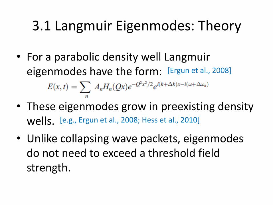
3.1 Langmuir Eigenmodes: Theory

• For a parabolic density well Langmuir eigenmodes have the form:

• These eigenmodes grow in preexisting density wells.

• Unlike collapsing wave packets, eigenmodes do not need to exceed a threshold field strength.

[Ergun et al., 2008]

[e.g., Ergun et al., 2008; Hess et al., 2010]

3.2 Langmuir eigenmodes fits

• Fits to eigenmode theory agree well with data for most localized waveforms.

• Eigenmodes provide a better explanation for localized waves than wave packet collapse.

Images from Graham et al., ApJL, 2012a. Both packets are below the collapse threshold.

[Ergun et al., 2008]

4.1 Electrostatic Decay: Theory

• Langmuir waves generated by electron beams have wave number

• These Langmuir waves can decay into backward propagating Langmuir waves: L → L’ + S.

• By assuming the linear dispersion relations

and the wave numbers are:

where

4.2 Doppler-shifted frequencies

• Langmuir waves are convected past STEREO at vsw.

• Therefore STEREO will observe waves at Doppler-shifted frequencies:

• The predicted Doppler-shifted frequency difference is:

• For ion-acoustic waves, the predicted Doppler-shifted frequency is: [Cairns and Robinson, 1992b;

Henri et al., 2009]

4.3 Langmuir/z-mode waves

• In a magnetized thermal plasma Langmuir waves connect to the magnetoionic z-mode wave to form the Langmuir/z-mode wave.

• Langmuir portion of the mode is electrostatic (E parallel to B0).

• Z-mode portion is electromagnetic (E perpendicular to B0).

• F = Eperp2/Etot

2 is the proportion of perpendicular energy density to total energy density.

[Willes & Cairns, 2000; Layden et al., 2011]

[Graham et al., 2012, JGR, submitted]

4.4 Decay of Langmuir/z-mode waves

• For kb > k0 Langmuir waves decay into Langmuir-like waves, implying small F.

• For kb ≤ k0 Langmuir waves decay into z-mode-like waves, implying large F.

• For decay of Langmuir waves to z-mode-like waves the Doppler-shifted frequency difference is:

• Z-mode waves can form for kb > k0 if multiple decays occur (i.e., an ES backscatter followed by a decay to z-mode waves).

4.5 Doppler-shifted frequencies versus vb/c

• Plot of Doppler-shifted frequencies versus vb/c for nominal solar wind conditions

• Dashed line is fp.

• Z-mode waves have frequencies near fp, so are difficult to distinguish from fL’

d.

fL’d

• vb/c is estimated by assuming electrons travel at constant speed along a Parker spiral.

fLd

4.6 Event selection

• We analyse Langmuir waveforms in type III source regions between 2009 June and 2012 February; a total of 596 events were selected.

• We also divide events into F < 0.2 and F > 0.2, corresponding to weak and strong perpendicular fields.

• Figure of F versus vb/c for Langmuir events with multiple distinct spectral peaks (86 events for F < 0.2, 145 events for F > 0.2).

• weaker Eperp are generally observed at lower vb/c.

4.7 Example of electrostatic decay (F < 0.2) • STEREO events on 2011

January 22.

• Panels: waveforms of Epar, wavelet transforms, and power spectra.

• Left: before ES decay.

• Right: during ES decay.

• Observed and expected frequency differences agree (360±80Hz versus 300±90Hz).

11:38:48.722 UT 11:38:39.207 UT [Graham and Cairns, JGR, 2012, submitted]

4.8 ES decay (F < 0.2) – general analysis

• Expected Δf calculated using:

• Observed and expected Δf agree well.

• When intense ion-acoustic waves are observed then Δf = fS as expected for ES decay.

• These results provide strong evidence for ES decay in type III source regions.

[Graham and Cairns, JGR, 2012, submitted]

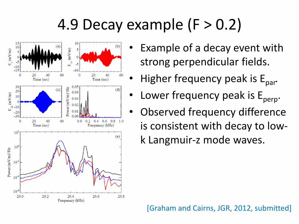
4.9 Decay example (F > 0.2)

• Example of a decay event with strong perpendicular fields.

• Higher frequency peak is Epar.

• Lower frequency peak is Eperp.

• Observed frequency difference is consistent with decay to low-k Langmuir-z mode waves.

[Graham and Cairns, JGR, 2012, submitted]

4.10 Decay to Langmuir/z waves (F > 0.2)

• Expected Δf calculated using:

• Observed and expected Δf agree well.

• When intense S waves are observed Δf = fS, as expected for ES decay to z-mode waves.

• These results provide strong evidence for decay to Langmuir/z-mode waves.

[Graham and Cairns, JGR, 2012, submitted]

4.11 ES decay and decay to Langmuir/z waves

• Power spectra at (a) vb/c = 0.05, (b) vb/c = 0.10, (c) vb/c = 0.18.

• For vb/c < 0.1 Langmuir waves undergo a single ES decay to backscattered Langmuir waves.

• For vb/c > 0.1 Langmuir waves generally decay to z-mode waves at low k.

• For vb/c ~ 0.1 three peaks similar to (b) are commonly observed.

- Epar

- Eperp [Graham and Cairns, JGR, 2012, submitted]

5. Discussion

• Approximately 35% of observed events appear to be localized, suggesting Langmuir eigenmodes.

• Approximately 40% of observed events are likely to be decay events.

• Langmuir eigenmodes can produce radio waves at fp and 2fp via the antenna mechanism [Malaspina et al., 2010, 2012].

• Transverse waves can be produced by coalescence L + L’ → T(2fp), EM decay L → T(fp) + S, or mode conversion of Langmuir/z-waves.

6. Summary

• Localized Langmuir waves (~ 35% of TDS events) are inconsistent with collapsing wave packets but are generally consistent with eigenmodes of density wells.

• ES decay of Langmuir-like waves to Langmuir-like and z-mode-like waves is commonly observed (~ 40 % of TDS events).

• Z –mode waves near k =0 are commonly observed (~ 25 % of TDS events)

• Both Langmuir eigenmodes and ES decay may be important in producing the radio waves observed in type III bursts. [Graham et al., ApJL, 2012; Graham et al., JGR, 2012; Graham and Cairns, JGR,

2012, submitted]

References • I. H. Cairns and P. A. Robinson, Geophys. Res. Lett., 19, 1069 (1992).

• I. H. Cairns and P. A. Robinson, Geophys. Res. Lett., 19, 2187 (1992).

• I. H. Cairns and P. A. Robinson, Geophys. Res. Lett., 22, 3437 (1995).

• R. E. Ergun et al., Phys. Rev. Lett., 101, 051101 (2008).

• D. B. Graham, O. Skjaeraasen, P. A. Robinson, and I. H. Cairns, Phys. Plasmas, 18, 062301 (2011).

• D. B. Graham, P. A. Robinson, I. H. Cairns, and O. Skjaeraasen, Phys. Plasmas, 18, 072302 (2011).

• D. B. Graham, I. H. Cairns, D. M. Malaspina, and R. E. Ergun, ApJL, 753, L18 (2012).

• D. B. Graham et al., J. Geophys. Res, 117, A09107 (2012).

• D. A. Gurnett et al., J. Geophys. Res, 86, 8833 (1981).

• P. Henri et al., J. Geophys. Res., 114, A03103 (2009).

• S. L. G. Hess, D. M. Malaspina, and R. E. Ergun, 115, A10103 (2010).

• A. Layden, I. H. Cairns, P. A. Robinson, and J. LaBelle, J. Geophys. Res.,116, A12328 (2011).

• D. M. Malaspina, I. H. Cairns, and R. E. Ergun, J. Geophys. Res., 115, A01101 (2010).

• D. M. Malaspina, I. H. Cairns, and R. E. Ergun, ApJ, 755, 45 (2012).

• P. A. Robinson, Rev. Mod. Phys., 69, 507 (1997).

• G. Thejappa, R. J. MacDowall, M. Bergamo, and K. Papadopoulos, ApJL, 747, L1 (2012).

• G. Thejappa, R. J. MacDowall, and M. Bergamo, Geophys. Res. Lett., 39, L05103 (2012).

• G. Thejappa, R. J. MacDowall, and M. Bergamo, J. Geophys. Res., 117, A08111 (2012).

• A. J. Willes and I. H. Cairns, Phys. Plasmas, 7, 3167 (2000).