Nonlinear Effects in Optical Fibers and...

SMR 1829 - 7

Winter College on Fibre Optics, Fibre Lasers and Sensors

12 - 23 February 2007

Nonlinear Effects in Optical

Fibers and Applications

Hugo L. Fragnito

Optics and Photonics Research Center UNICAMP-IFGW

Brazil

Nonlinear Optics

H.L. Fragnito 1

13/2/2007 H.L. Fragnito 1

Nonlinear Effects in Optical

Fibers and Applications

Prof. Hugo L. Fragnito

Unicamp - IFGW

Nonlinear Optics:

Optical phenomena resulting from interactions of matter with

radiation at high optical intensities

Goals:

To provide a background on fundamentals and overview of basic

nonlinear optical processes that occur in glasses, emphasizing those

most relevant to optical fiber communications and fiber-optic devices


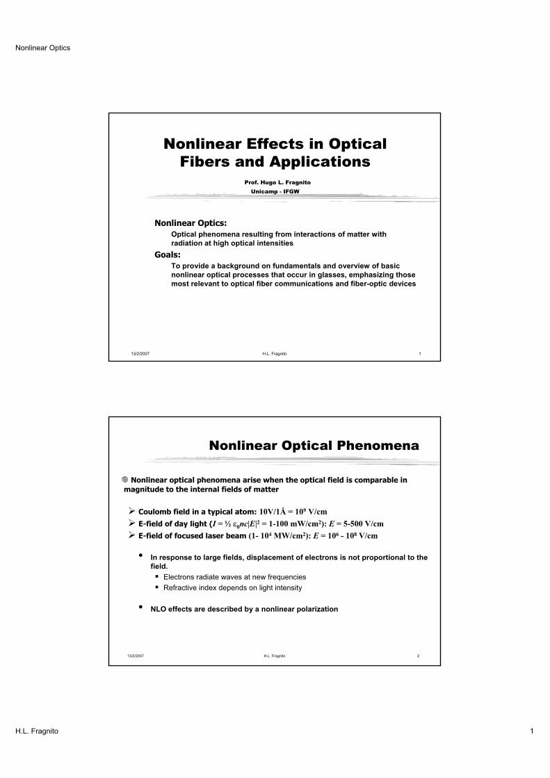
Nonlinear Optical Phenomena

Nonlinear optical phenomena arise when the optical field is comparable in

magnitude to the internal fields of matter

Coulomb field in a typical atom: 10V/1Å = 109 V/cm

E-field of day light (I = ½ 0nc|E|2 = 1-100 mW/cm2): E = 5-500 V/cm

E-field of focused laser beam (1- 104 MW/cm2): E = 106 - 108 V/cm

• In response to large fields, displacement of electrons is not proportional to the

field.

Electrons radiate waves at new frequencies

Refractive index depends on light intensity

• NLO effects are described by a nonlinear polarization

Nonlinear Optics

H.L. Fragnito 2


Optical Polarization

Dipole moment per unit volume

Vol/jjrqNP

),(),(1

2

2

02

2

2trP

ttrE

tc

Source term of wave equation

The polarization describes all optical phenomena


Nonlinear polarization

Optical susceptibilities

Linear polarization: PL = P(1) = 0(1)E

Second order: P(2) = 0(2)E2

Third order: P(3) = 0(3)E3

nth order: P(n) = 0(n)En

...][ 3)3(2)2()1(

0 EEEP

(Rigorous definitions will be presented later)

)3()2()1( PPPPPP NLL

(n) : Optical susceptibility of nth order

In centrosymmetric media

(3) is the lowest order

nonlinearity in glasses,

liquids,…

0)()( )2( nEPEP

Nonlinear Optics

H.L. Fragnito 3


Third Order Nonlinear Optics:

Effects that occur in any material (not necessarily non-centro-

symmetric crystals) such as glasses, liquids, gases...

A quick tour through the catalog of third order

nonlinear optical effects


Third harmonic generation & optical Kerr effect

E E e c ci t12 0 . .

P E e c ci t3

3 18 0

303 3( ) ( ) . .

P E E e c ci t( ) ( ) | | . .3 38 0

30

20

3

(3) medium

E E e E e c ci t i t12 1 2

1 2( . .)

2 - 1(3) medium

Sum and difference frequency generation

2 + 1

Third order nonlinearities

refractive index change

Nonlinear Optics

H.L. Fragnito 4


dc Kerr effect

Edc: dc or low frequency (<< optical frequency )

Quadratic electro-optic effect

E E E e c cdci t( . .)1

2 0

P E E e c cdci t1

2 01 3 2

03( ) . .( ) ( )

n n n

n E ndc

0

3 203 2( ) /

Control VoltageV

dLiquid cell

Edc = V/d

Discovered by J. Kerr (1875) and used since 1940’s in

high speed photography

(nanosecond switching time, but needs kVolts)


Optical Kerr effect

Self effect..02

1 cceEE ti..|)|( 0

2

0

)3(

43)1(

021 cceEEP ti

InEnn 2

2

0

)3(

83 ||

0

More convenient description n = n0 + n2 I

Irradiance (W/cm2) || 2

00021 EcnI

Example: glasses n2 = 10-15 cm2/W, n0 = 1.5, I = 100 MW/cm2 n = 10-7

Note: = 2 n (l / ) and factor (l / ) can be very large

Pump induced effect

.).( 021 cceEeEE titi

pp ..|)|( 0

2)3(

23)1(

021 cceEEP ti

p

ppnInEn 2

2)3(

43 2||

0

Nonlinear Optics

H.L. Fragnito 5


Self phase modulation

Spectral broadening of short pulses

(t)I(t)0 2n z

cI t( )Phase shift

0( )tn z I

t0

22

Instantaneous frequency

n I

ct p

2 max

Spectral broadening

Example: SiO2, = 1 µm, n2 = 3 10-16 cm2/W, = 1 cm,

tp = 50 fs, Imax = 2 1011 W/cm2 = 40 nm

time, t

13/2/2007 H.L. Fragnito 10

Four wave mixing

Three incident waves + one generated

(3)

k1k4

k2

k3

4 1 2 3

4 1 2 3k k k k

( ; )E E E E

degenerated FWM: 4 = 1 = 2 = 3 =

)(*

321

)3(

083)3( 4 rktieEEEP

P E E E e c ci t k r( ) ( ) ( )

. .3 34 0

31 2 3

4 4

Nonlinear Optics

H.L. Fragnito 6

13/2/2007 H.L. Fragnito 11

Laser induced gratings

• Two interfering waves induce a grating (refractive or absorptive)

• Moving grating:

• grating moves with velocity

• inelastic scattering

• A third wave scatters (diffracts) in the grating

(grating period) 2 /| |k

k1

k2

k k k1 2

k k

k k

k

(stationary grating)

k|

k k;

k;

k k;

13/2/2007 H.L. Fragnito 12

Four Wave Mixing (FWM) in fibers

Important effect for WDM systems

Reduces the transmitted power in each channel

Produces cross talk

P

P1 P2

P

1 2

1 22 1

Nonlinear Optics

H.L. Fragnito 7

13/2/2007 H.L. Fragnito 13

Beating of input waves induces a (moving) index grating

A third wave suffers inelastic diffraction

The pump waves are also (Self) diffracted

z

2 /

Aei t z( )

FWM as self-diffraction

P

P1 P2

P

1 2

1 2

.).(|||| )(*

21

2

2

2

1

)3(

43

0cceEEEEn zti

n

13/2/2007 H.L. Fragnito 14

FWM and Phase Matching

Generic case of FWM: ijk i j k

Wavevector (including SPM and XPM):

FWM efficiency:

• Very useful for physical insights and rather good estimates

• One of the input tones can be noise: MI, noise amplification,...

Wavevector mismatch

LLPP eff

ik

kii /2)(

2

2

22

2

1

)2/(sin41

L

L

e

Le

/)1( L

eff eL

LLPP eff

ik

kiijijkk /2)()()()(

Propagation constant

( = loss coefficient)

Nonlinear Optics

H.L. Fragnito 8

13/2/2007 H.L. Fragnito 15

Phase conjugation

Degenerate four wave mixing with two counter-propagating pump beams

and a weak signal beam

F B

F Bk k

Spatial phase conjugate

of signal field

k F (3)

kBk

k k4

P E E E e c cF Bi t k k k rF B F B( ) ( ) [( ) ( ). ]

. .3 38 0

3

P E E E e e c cF Bik r i t( ) ( ) . .3 3

8 03

In fibers can be used to compensate dispersion and other

time-phase distortions

13/2/2007 H.L. Fragnito 16

Phase conjugate mirror

Reflected wave returns on itself

Correction of phase front

distortions by PC mirror

aberration free

reflected wave

PC mirror

Conventional

mirror

Aberrating

medium PC mirror

Nonlinear Optics

H.L. Fragnito 9

13/2/2007 H.L. Fragnito 17

Nonlinear absorption

Single photon resonance

Gain saturation (Lasers)

Saturation of absorption

Near resonances (n) is complex ( i )

Absorption is described by (2n-1) (odd orders)

En

erg

y

ground

excited

)||(||2

2)3(

43)1(20 EE

t

PE

Time averaged absorbed power per unit volume

Absorption coefficient

ncE( | | )( ) ( )1 3

43 2

( )( )3 0

( )( )3 0

13/2/2007 H.L. Fragnito 18

Two photon absorption

”(3) process ITPA

TPA coefficient

Typically, TPA = 10-10 cm/W

22

0

)3(

2

3

cnTPA

Nonlinear Optics

H.L. Fragnito 10

13/2/2007 H.L. Fragnito 19

Stimulated Scattering

(Spontaneous) Scattering Spectrum

0

Rayleigh

Brillouin

RamanRaman

Stokes

( 0)

anti-Stokes

( 0)

Rayleigh wing

1000 cm-1

5 cm-1

5 cm-1

0.1 cm-1

Lasers can excite strong material

oscillations. Scattered light wave interfere

with the laser possibly reinforcing the

material excitation, thus leading to positive

feedback: stimulated scattering.

Raman: Vibrations/Optical phonons

Brilluoin: Sound waves/Acoustic phonons

Rayleigh wing: Orientational fluctuations

(liquids)

Rayleigh: Density (entropy) fluctuations

13/2/2007 H.L. Fragnito 20

Stimulated Brillouin Scattering

(SBS)

Backward scattering

S = P - B

P

Typical Frequency shift:

B 50 GHz (glasses)

B P (sound velocity/light velocity)

Bandwidth B 20 - 100 MHz

Gain intensity factor gB ~ 10-9 - 10-8 cm/W (glasses)

B

laser

B

thLg

I 121

Threshold:

Coupling to acoustic waves,

acoustic phonons

Acoustic resonance

z

IP IS

~ 10 MW/cm2

= loss coefficient)

Seed to initiate process

comes from

spontaneous scattering

seedIIgdz

dISPB

S )(

(L ~ 1 m)

Measurem.

Lorentzian

Nonlinear Optics

H.L. Fragnito 11

13/2/2007 H.L. Fragnito 21

Electrostriction

Electric field gradient attracts polarizable molecules.

Driving force for acoustic waves (SBS), self focusing,..

Force/Volume: 2

021 ENuf

Density change: 12

2C Ee

Compressibility

Cp

1 910 m / N2

Electrostriction coefficient

e n n13 0 0

2021 2( )( )

E

Refractive index change:

n Enn n

C

0 02

02

22 1

72 02

( )( )

Pressure: p EU 12

2

In glasses, shear acoustic waves may play a role (specially in waveguides)

(take time average over 1 optical cycle) :

2

12 442 ,el Ef E E

13/2/2007 H.L. Fragnito 22

Brillouin frequency

In bulk

incident

scattered

acoustic

In fibers

incidentscattered

acoustic

Max. freq. ( ) B = 12 GHz in silica

Max. freq. B = 11 GHz in silica

Transverse k: acnkT /)/( 22

1

cnVVkkV SSoptacSac /22max

cVnVkV SeffSoptacSB /22

)2/sin()2/sin(2)( max

acSoptacSac VkkV

Dainese et.al., Nature Phys. 2006

Nonlinear Optics

H.L. Fragnito 12

13/2/2007 H.L. Fragnito 23

Forward Brillouin scattering

In waveguides ~ transverse acoustic waves can “resonate” with cladding

reflections

Min. freq. B = 20 MHz in 125 um

cladding fibers.

Max freq ~ 400 MHz.

Min. freq. B = 2 GHz in 1 um PCF

cladSacSac dVkV /

dcladd

d = 1.2 mDainese et.al., Opt. Express 2006

13/2/2007 H.L. Fragnito 24

Impulsive Brilouin Scattering

Short pulse excites transverse acoustic wave packets that reflects at cladding interface

A weak probe senses refractive index changes each time the wave packet crosses the fiber core (round trip time ~10 ns)

In solid core PCFs (1 um diam) the round trip time is much shorter

Dainese et.al., Opt. Express 2006

Mouza et.al., PTL 1998Conventional 125 um cladding fiber

PCF 1.2 um core diam.

Nonlinear Optics

H.L. Fragnito 13

13/2/2007 H.L. Fragnito 25

Stimulated Raman Scattering (SRS)

Forward Scattering

Coupling to molecular vibrations, optical phonons

Frequency shift

R ~ 200 – 500 cm-1

Bandwidth

~ 1 GHz (gases) – 5 THz (glasses)

S = P - R

PIP IS

Threshold: ~ 1 GW/cm2

Gain intensity factor gR ~ 10-12 - 10-8 cm/W

seedIIgdz

dISPR

S )(

LgI

R

th

16

(L ~ 1 m)

13/2/2007 H.L. Fragnito 26

Formal Theory of Nonlinear Optics

Goals:Understand the general properties of (3)

• Symmetries

• Frequency dependencies

• What (3) describes a given NLO effect

Conventions to facilitate reading of literature on NLO

• Different systems of units

Nonlinear Optics

H.L. Fragnito 14

13/2/2007 H.L. Fragnito 27

Theory of nonlinear susceptibilities

Let us start with the linear susceptibility:

What is the most general linear relation between two vector fields (P and E)?

Then:

What is the most general nonlinear relation between two vector fields (P and En)?

13/2/2007 H.L. Fragnito 28

),(),,,(),( )1(3

0

)1( trEtrtrrdtdtrPV

Linear constitutive relation

Time domaintensor (3x3 elements)

tttt for0)()1(

),(),(),( )1(

0

)1( trEttrtdtrP

),()(),( )1(

0

)1( trEtttdtrP

Reality

Time and space invariance

Causality

Locality(good approximation)

Homogeneous media

Most general linear relation between vector functions:

Response function

),(),,,( )1()1( ttrrttrr

Properties of the response function E t A t( ) ( )

P t A t( ) ( )( ) ( )10

1

time, t0

memory time

realis)(realare)(and)( ttEtP

Nonlinear Optics

H.L. Fragnito 15

13/2/2007 H.L. Fragnito 29

Linear susceptibility

Things are more simple in the frequency domain:

Constitutive relation in the frequency domain

dtte ti )()( )1()1(

P E( ) ( )( ) ( ) ( )10

1

Fourier transform pair (convention)

Susceptibility is a frequency domain concept

dttEeE ti )()( dEetE ti )()(21

13/2/2007 H.L. Fragnito 30

Properties of susceptibility

)()(

)/()()( 1 d

)/()()( 1 d

)1(2 1)( in

11 222 nn

n2

Causality of (t)

Kramers-Krönig relations

(Hilbert transform pair)

Reality of response function ( (t))

Complex refractive index

(take Cauchy principal value of integrals)

n = refractive index

= extinction coefficient

(absorption coefficient )

Complex function )()()( i

FIR IR VIS UV

0

1

Nonlinear Optics

H.L. Fragnito 16

13/2/2007 H.L. Fragnito 31

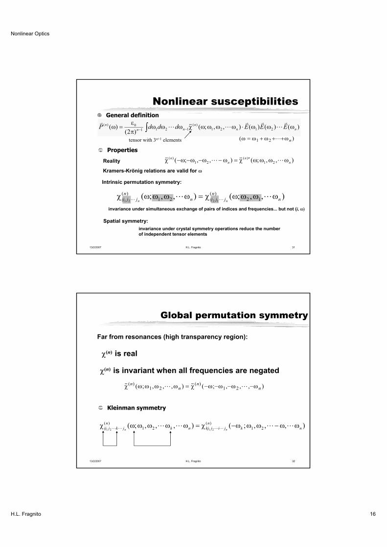
Nonlinear susceptibilities

Reality

( )1 2 n

)()()(),,;()2(

)( 2121

)(

1211

0)(

nn

n

nn

n EEEdddP

tensor with 3n+1 elements

),,;(),,;( 21

)(

21

)(

n

n

n

n

),,;(),,;( 12

)(

21

)(

1221 n

n

jjijn

n

jjij nn

invariance under simultaneous exchange of pairs of indices and frequencies... but not (i,

Kramers-Krönig relations are valid for

Intrinsic permutation symmetry:

Spatial symmetry:

invariance under crystal symmetry operations reduce the number

of independent tensor elements

Properties

General definition

13/2/2007 H.L. Fragnito 32

Global permutation symmetry

Kleinman symmetry

),,,;(),,,;( 21

)(

21

)(

2121 nk

n

jijkjnk

n

jkjij nn

Far from resonances (high transparency region):

(n) is real

(n) is invariant when all frequencies are negated

( ) ( )( ; , , , ) ( ; , , , )nn

nn1 2 1 2

Nonlinear Optics

H.L. Fragnito 17

13/2/2007 H.L. Fragnito 33

Third order susceptibility (3)

Reality of E and P

)( 321Tensor, 81 elements

),,;(),,;( 321

)3(

321

)3(

),,;(),,;( 312

)3(

321

)3(

ikjlijkl

Intrinsic Permutation Symmetry

Properties

Far from any resonance

Global Permutation Symmetry (Kleinman symmetry)

)()()(),,;()2(

)( 321321

)3(

212

0)3( EEEddP

),,;(),,;( 312

)3(

321

)3(

jkilijkl

13/2/2007 H.L. Fragnito 34

General form

Third harmonic generation:

(3) for isotropic media

xxxx = yyyy = zzzz

yyzz = zzyy = zzxx = xxzz = xxyy = yyxx

yzyz = zyzy = zxzx = xzxz = xyxy = yxyx

yzzy = zyyz = zxxz = xzzx = xyyx = yxxy

xxxx= xxyy + xyxy + xyyx

• Only 21 non vanishing elements

and only 3 independent elements

xxxx = 3xxyy = 3xyxy = 3xyyx

ijkl ij kl ik jl il jk( ) ( ) ( ) ( )3

11223

12123

12213

• Far from any resonance (Kleinman

symmetry valid): only one independent

element

11223

12123

12213 3( ) ( ) ( ) ( ; , , )

• Only one independent element

Nonlinear Refractive index: 11223

12123( ) ( ) ( ; , , )

• Only two independent elements

ijkl ij kl ik jl il jk( ) ( ) ( )( ; , , ) ( )3

11223

12213

Nonlinear Optics

H.L. Fragnito 18

13/2/2007 H.L. Fragnito 35

Maker-Terhune Coefficients

General expression of nonlinear polarization for monochromatic

field (frequency ) in isotropic medium

*

021*

0

)3( )()()( EEEBEEEAtP

• Effective “linear” tensor

)3(

122123

)3(

112223

B

A

.).(isfieldActual21 cceE ti

EP 0

ij ij i j j iA B E B E E E E( )| | ( )* *12

2 12

• Molecular orientations: B/A = 3• Non-resonant electronic: B/A = 1• Electrostriction: B/A = 0

P.D. Maker and R.W. Terhune, Phys. Rev. 137, A801 (1965).

13/2/2007 H.L. Fragnito 36

Ellipsoid rotation

Arbitrary polarized field as a sum of left (-) and right (+) circularly polarized waves

E E E 2/ˆˆˆ yix

x

y

zx

y

P E0 A E A B E| | ( )| |2 2Then:

and the refractive index difference for the two circularly polarized waves is

nB

n cI I

0 02

( ) (depends on B only)

The polarization ellipse rotates by an angle 12

n z c/

x

y z=0

z=zk

Nonlinear Optics

H.L. Fragnito 19

13/2/2007 H.L. Fragnito 37

Circularly vs. linearly polarized waves

Circularly polarized waves

E E E E or

x

y

nA

n cIcircular circular

0 02

E E=n

A B

n cIlinear linear

/ 2

0 02

Linearly polarized waves y

x

• Molecular orientations: nlinear / ncircular = 4• Non-resonant electronic: nlinear / ncircular = 3/2• Electrostriction: nlinear / ncircular = 1

13/2/2007 H.L. Fragnito 38

Physical origin of n2

Physical mechanism n2 (cm2/W) response time

Electronic (non-resonant) 10-16 fs

Molecular orientation 10-14 ps

Electrostriction 10-14 ns

Thermal 10-6 ms

Population (resonant) 10-10 ns

Medium n2 (cm2/W) response time

Air 10-19 fs

SiO2 glass 3x10-16 < 1 fs

CS2 10-14 2 ps

GaAs 10-6 20 ns

CdSe doped glasses 10-13 30 ps

Polydiacetylene (resonant) 10-8 2 ps

Polydiacetylene (non-resonant) 10-12 fs

Examples

Nonlinear Optics

H.L. Fragnito 20

13/2/2007 H.L. Fragnito 39

Monochromatic fields

..)( 0

021 cceEtE

ti )()()( 0000 EEE

..)( 0321

4

)()()()3(

021)3( cceEEEtP

ti

eff

Laser fields are monochromatic

Mixing of monochromatic waves

generation of wave at 4 = 2 2 - 1

Examples:

),,;()( 2214

)3(

43

4

)3(

eff

THG: 3 = + ),,;3()3( )3(

41)3(

eff

generation of wave at 4 = 2 1 + 2),,;()( 2113

)3(

43

3

)3(

eff

)+=( 3214

Self phase modulation

Cross phase modulation

),,;()( 1111

)3(

43

1

)3(

eff

),,;()( 2211

)3(

23

1

)3(

eff

DC Kerr effect )0,0,;(3)( 11

)3(

1

)3(

eff

13/2/2007 H.L. Fragnito 40

Systems of units

Système Internationale, SI Gauss [esu(q)]

P En n0

( ) P En n( )

D E P E0 D E P E4

n 1 n 1 4

( ) * ( )[( / ) ] / ( ) ( )n n n nm V esu1 4 14 3 10

electric charge

susceptibilities

(3* = 2.9979...)

constitutive relations

refractive index

electric field E (V/m) = 3* 104 E(esu)

1 C = 3* 109 esu

Nonlinear Optics

H.L. Fragnito 21

13/2/2007 H.L. Fragnito 41

Alternative definitions

Different definitions, conventions and units

E t E e c ci t( ) . . = 0

dtetEE ti)(=)( take complex conjugate of (n)

dtetEE ti)(=)(21

divide P(n)( ) by (2 )n-1

divide (n) by 2n-1

P d EEi il l( ) ( )2 = divide d by 0

P E Enn

n n( ) ( ) ( ) ( )( )1 0

1 substitute by eff

Convert to SI units before designing experiments

deEtE ti2)(=)( do nothing

012

2 2 16

3 3( )( ) ( )E E Eloc loc loc divide (n) by n

13/2/2007 H.L. Fragnito 42

Hyperpolarizability

Induced dipole moment per molecule

0 Eloc P N

Polarizability of molecule

In dilute media (gases), metals, and semiconductors Eloc = E and (n) N (n)

Nonlinear case

02 2 3 3E E Eloc loc loc

( ) ( )

Second order hyperpolarizability

Third order hyperpolarizability

Linear case

The (local) field acting on a molecule differs from the macroscopic field.

Nonlinear Optics

H.L. Fragnito 22

13/2/2007 H.L. Fragnito 43

Local field

Relation between local field acting on the molecule and macroscopic field

Isotropic medium

Local field

correction factor

Linear case

Lorentz-Lorenz

f n2 23

13

2

23

1

2N

n

n

P N Eloc0

E E Ploc / 3 0

E f Eloc

13/2/2007 H.L. Fragnito 44

Local field correction

Nonlinear case

Total polarization at

Second order

hyperpolarizability

Nonlinear polarization at

General case

Use local field factors to convert hyperpolarizability

(microscopic) into susceptibility (macroscopic)

P N E P E f Ploc0 01( )

P f PNL( ) ( ) ( )

P N E Eloc loc( ) ( ; , ) ( ) ( )( )0

21 2 1 2

P f f f N E E( ) ( )( ) ( ) ( ) ( ) ( ; , ) ( ) ( )21 2 0

21 2 1 2

( ) ( )( ; , , ) ( ) ( ) ( ) ( ; , , )nn

nnf f f N1 1 2 1

Nonlinear Optics

H.L. Fragnito 23

13/2/2007 H.L. Fragnito 45

Quantum mechanics theory of NLO

Goals:

Understand the connection of (n) to microscopic properties of

material systems

NLO effects due to the dependence of populations on intensity

Physical origin of (n)

Insights on what makes one material to be more nonlinear than

another

Importance of resonance and relaxation

13/2/2007 H.L. Fragnito 46

Density matrix

Statistical quantum mechanics

Expectation of any physical observable such as P

)(0 tEHH],[Htt

i

Eiil lkjllkjljkjktt

)(

/)( kkjjjk HH

is the density operator, given by the Liouville Equation

)(kj jkkjNTrNNP

Hamiltonian

Interaction potential

Relaxation (incoherent interactions, such as collisions)

Nonlinear Optics

H.L. Fragnito 24

13/2/2007 H.L. Fragnito 47

Relaxation

Form of relaxation term should restore thermal equilibrium:

Diagonal elements: populations

Non diagonal elements: coherences

j kjkkjjjkkk

t

En

erg

y

ji

kj

| i

| j

| k

ij

Boltzmann distribution

jk = Incoherent (spontaneous) transition rate j k

jkjk

jk

t

jk

e

jjkj

e

kkPrinciple of Detailed Balance

Postulate of Random Phases )(0 kje

jk

nne E kTe n /

jk = kj (since must be hermitian)

13/2/2007 H.L. Fragnito 48

Perturbation theory

Perturbative expansion

],[],[ )1()(

0

)( nnn

ttEHi

)2()1(e

nn E)()(

Solve by iterations

Nonlinear polarization )( )()( nn TrNP

Note: expressions must be corrected for1) local field (dielectrics)

2) orientational averaging (amorphous & fluids)

3) inhomogeneous broadening (ex., Doppler effect)

Nonlinear Optics

H.L. Fragnito 25

13/2/2007 H.L. Fragnito 49

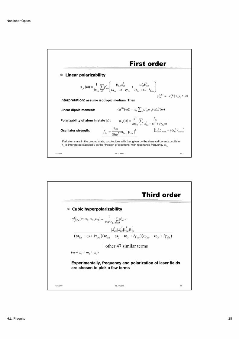
First order

Linear polarizability

)()()( 0

)1( Ea a

e

aaLinear dipole moment:

2

2||

3

2bababa

e

mf

Polarizability of atom in state |a

Oscillator strength:

b baba

baa

i

f

m

e22

0

2

)(

If all atoms are in the ground state, coincides with that given by the classical Lorentz oscillator.

fba is interpreted classically as the “fraction of electrons” with resonance frequency ba

Interpretation: assume isotropic medium. Then

ab baba

k

ba

j

ab

baba

k

ab

j

bae

aajkii0

1)(

azyxbeba |,,|3,2,1

orient

2

31

orient

2

baba rx

13/2/2007 H.L. Fragnito 50

Third order

Cubic hyperpolarizability

))()(( 332 dadacacababa

l

ca

k

ca

j

bc

i

ab

iii

( = 1 + 2 + 3)

Experimentally, frequency and polarization of laser fields

are chosen to pick a few terms

jklm aae

abcd

( ) ( ; , , )!

31 2 3 3

0

1

3

+ other 47 similar terms

Nonlinear Optics

H.L. Fragnito 26

13/2/2007 H.L. Fragnito 51

Two Photon Resonances

Types of resonances of (3)

v

2 1

Raman resonancevibration

ba2

1

TPA resonance

Two photon absorption Electronic

transition

(There are many other types of resonances in the 48 terms of (3))

13/2/2007 H.L. Fragnito 52

NLO from populations

Intensity dependent populations

Nonlinear oscillator

Perturbation theory fails

Example: Two level system:

cannot be expanded in power series for I Isat

Populations must be calculated from rate equations

Quantum harmonic oscillator:

oscillator strengths

polarizabilities are equal for all levels!

LINEAR!

Nonlinearity is related to anharmonicity of potential

P N I Enn nn0 ( )

NN

I I

e

sat1 /

f n nnk n k n k n1 11, ,( )

P N E I N Ennn0 0( )

Nonlinear Optics

H.L. Fragnito 27

13/2/2007 H.L. Fragnito 53

Optical Stark Shift

Energy shift due to difference

in polarizabilities of two states

polarizabilities pump field

Two level system:

b a

bap

ba

p ba ba

bap

ba Transition is always

pushed away from

resonance

pbaba

14 0

2( )b a pE

12 0

2

2 2

2 23a p

ba ba p p

ba p

EE( )

[( ) ]

| a

| b

13/2/2007 H.L. Fragnito 54

Non-resonant electronic n2

Result from quantum mechanics 11113 3 3( ) ( ) ( )( ; , , ) S T

TN gn

xnpx

pmx

mgx

ng pg mgmnp g

( )

( ) ( )( )( )

3 8

3 03

2

SN gn

xngx

gpx

pgx

ng pg pgpn

( )

( )( )( )

3 8

3 03 Single photon resonance

Two photon resonance

gn ng

k

np

j

gn

jkp

0

,3

1

SN xx( ) | |3 12

20

TN p xx

pgp g

( ) ,| |3 242

0

2

Optical Stark Shift

pgpg/2( )3

0

positive n2

negative n2

Nonlinear Optics

H.L. Fragnito 28

13/2/2007 H.L. Fragnito 55

Summary

Susceptibility is a frequency domain concept

Symmetries greatly simplify the form of tensors

Be aware of the definitions, conventions and unit system used in consulted references

Quantum mechanics gives a microscopic description of nonlinear optics

Use local field corrections to calculate susceptibilities from hyperpolarizabilities

Resonance enhancement of nonlinearities

Single photon resonance: Optical Stark Shift

Two photon resonances: Two photon absorption, Raman resonance

13/2/2007 H.L. Fragnito 56

Linear pulse propagationDefinitions

Wave equation in the frequency domain

Dispersion, Chirp

Example: gaussian pulse

Nonlinear pulse propagation in n2 mediaNonlinear Schrödinger equation

Self Phase Modulation, spectral broadening and chirp

Solitons

Propagation regimes

Nonlinear Pulse Propagation in Fibers

Prof. Hugo L. Fragnito Unicamp - IFGW

Nonlinear Optics

H.L. Fragnito 29

13/2/2007 H.L. Fragnito 57

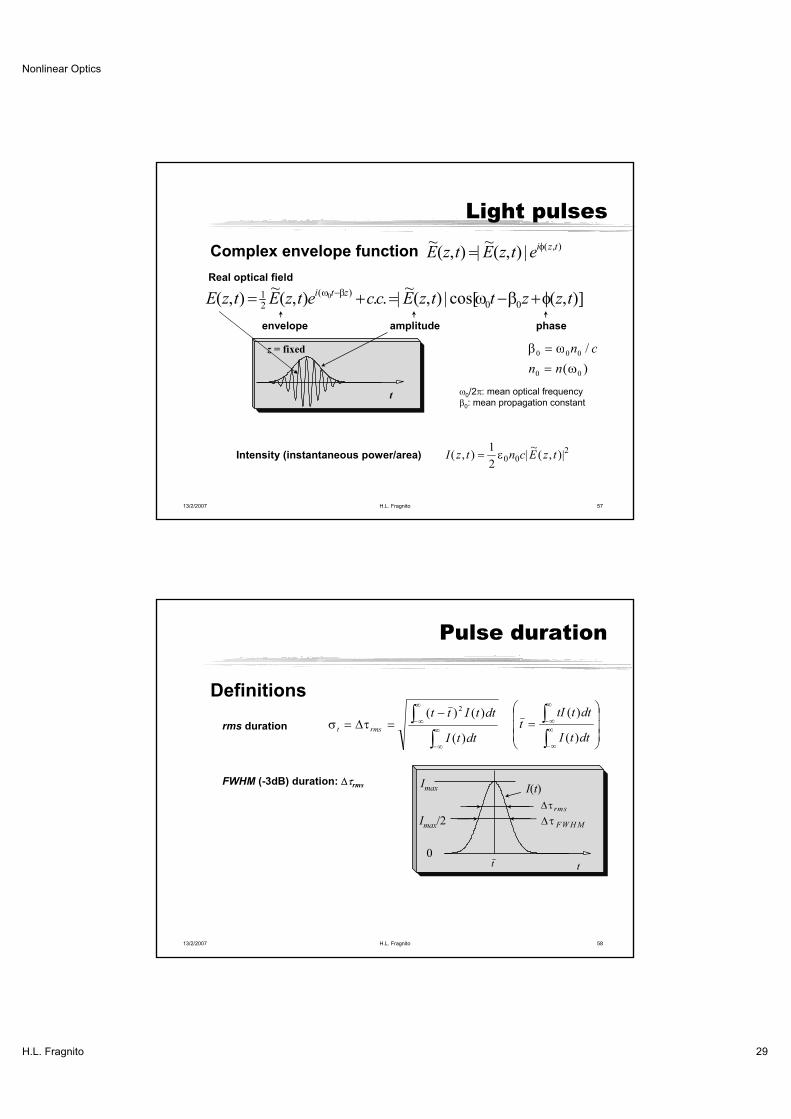
Real optical field

Complex envelope function

)],(cos[|),(~

|..),(~

),( 00

)(

21 0 tzzttzEccetzEtzE

zti

envelope phaseamplitude

t

z = fixed

I z t n c E z t( , ) |~

( , )|1

20 0

2Intensity (instantaneous power/area)

)(

/

00

000

nn

cn

Light pulses

0/2 : mean optical frequency

0: mean propagation constant

),(|),(~

|),(~ tzietzEtzE

13/2/2007 H.L. Fragnito 58

Pulse duration

rms duration

Definitions

dttI

dttItt

rmst

)(

)()( 2

dttI

dtttIt

)(

)(

t

rms

FW H M

t

I(t)

0

Imax

Imax/2

FWHM (-3dB) duration: rms

Nonlinear Optics

H.L. Fragnito 30

13/2/2007 H.L. Fragnito 59

Wave propagation

General wave equation

Time domain

),(),(1

2

2

02

2

2trP

ttrE

tc

),(),(1

2

2

02

2

2

2 trPt

trEtc

Transverse waves

Isotropic media

Approximate in crystals

Problem: this equation is in the frequency domain, but the

constitutive equation is easier in the frequency domain

Frequency domain

),(),(),(),( 2

0

)1(

2

22

02

22 rPrE

crPrE

cNL

),(),()/( 2

0

22 rPrEcn NL

1)()( 2n

13/2/2007 H.L. Fragnito 60

ziezAyxrE )(),(),(),(

zi

NL erPz

Ai

z

AcnA yx ),(2)/( 2

02

2222

,

= 0 (since

is a mode)

0 (slowly varying

function of z)

1),,(2dxdyyx

The optical field has the form of a mode, (x,y)

The mode amplitude can be normalized such that

Substituting in the wave equation

Multiply by *dxdy and integrate

dxdyyxrPez

Ai NL

zi ),(*),(2 2

0

( also depends on frequency)

Wave equation in waveguides

Nonlinear Optics

H.L. Fragnito 31

13/2/2007 H.L. Fragnito 61

Most relevant (3) term for fibers

Analytical representation

0for0

0for)(2)(

EE

3rd order sum term

)(ˆ)(ˆ)(;)()()( *

21*

21 tPtPtPtEtEtE

Only positive frequencies need be considered

),,;( 321

)3()3(

SUM

)()()()()()()( 3

*

21

)3(

21043

321

)3(

21041)3( EEEddEEEddP DIFSUM

3rd order difference term ),,;( 321

)3()3(

DIFdescribes FWM, n2, SBS,

SRS (everything that is most

relevant in fibers).

describes THG and high

frequency sum generation

13/2/2007 H.L. Fragnito 62

No (3) dispersion

If the input field spectrum is narrow-band we can ignore the

frequency dependence in (3) (valid far from resonances)

2121

*

21

)3(

043)3( )()()()( ddEEEP

The nonlinear polarization is remarkably simple in the time

domain…

But, WARNING, this is true for nonresonant electronic (3). (Not true

for electrostriction, Raman, Brillouin,… if the field spectrum is

broad – such as fs pulses or DWDM systems).

(use convolution theorem)

)(|)(|)( 2)3(

043)3( tEtEtP

Nonlinear Optics

H.L. Fragnito 32

13/2/2007 H.L. Fragnito 63

SVEA

Slowly Varying Envelope Approximation

E z t E z t e c ci t z( , )~

( , ) . .( )12

0 0

~~

~~E

tE

E

zE0 0 and

Envelope varies very little in time over one optical period

or in space over one wavelength

13/2/2007 H.L. Fragnito 64

Wave equation in frequency domain

),(),( 2

02

2

2

2

zPzEcz

P z n E z( , ) [ ( ) ] ( , )02 1

Transparent, homogeneous and isotropic media

( ) ( ) /n c

Exact solution

Dispersion relation

E z E e i z( , ) ( , ) ( )0

Linear Propagation

1)()( 2n

Fourier transform

dttEeE ti )()( dEetE ti )()(21

Nonlinear Optics

H.L. Fragnito 33

13/2/2007 H.L. Fragnito 65

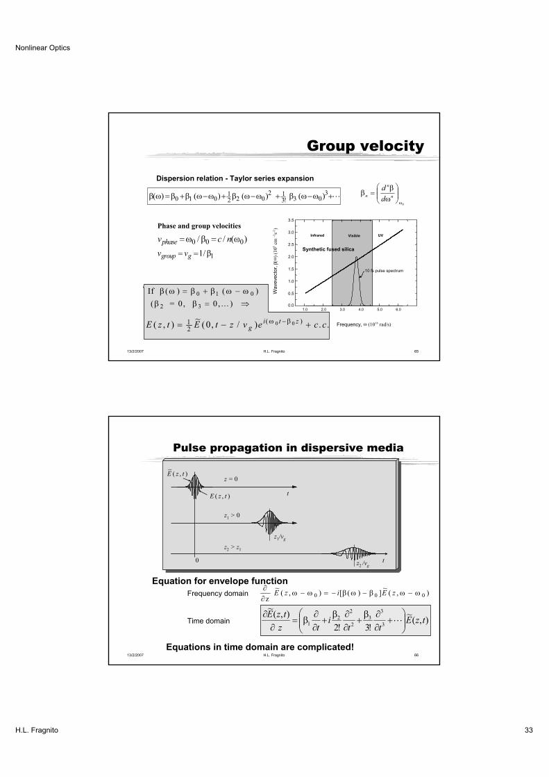
Group velocity

( ) ( ) ( ) ( )!0 1 0

12 2 0

2 13 3 0

3

Dispersion relation - Taylor series expansion

0

n

n

nd

d

1.0 2.0 3.0 4.0 5.0 6.00.0

0.5

1.0

1.5

2.0

2.5

3.0

3.5

10 fs pulse spectrum

UVInfrared Visible

Synthetic fused silica

Wavevecto

r,(

) (1

05

cm -1

s-1)

Frequency, (1015 rad/s)

v c nphase 0 0 0/ / ( )

v vgroup g 1 1/

Phase and group velocities

If

( = 0 , ... ) 2 3

( ) ( )

,

0 1 0

0

E z t E t z v e c cgi t z( , )

~( , / ) . .( )1

20 0 0

13/2/2007 H.L. Fragnito 66

Pulse propagation in dispersive media

t

t

z = 0

z1 > 0

0

z1/vg

z2 > z1

z2 /vg

~( , )E z t

E z t( , )

Equation for envelope function

z

~( , ) [ ( ) ]

~( , )E z i E z0 0 0Frequency domain

Time domain ),(~

!3!2

),(~

3

3

3

2

2

21 tzE

tti

tz

tzE

Equations in time domain are complicated!

Nonlinear Optics

H.L. Fragnito 34

13/2/2007 H.L. Fragnito 67

Dispersion parameter

Used in fiber optics

Dispersion parameter:

Received pulsesInput pulses with

different wavelengths

time

Optical fiber

Length L

++

DL

1[ps/nm/km]

202

2 cDRelation between D and 2:

13/2/2007 H.L. Fragnito 68

GVD in silica

0.4 0.6 0.8 1.0 1.2 1.4 1.6 1.8

-1000

-800

-600

-400

-200

0

Anomalous GVD

region

Normal GVD

region

Gro

up

ve

locity d

ispe

rsio

n,

D(p

s/n

m/k

m)

Wavelength, (µm)

Synthetic fused silica

Optical fibers for communications are made of silica

Transparent materials exhibit a particular ZD where D( ZD) = 0.

In pure silica, ZD = 1.27 µm (Zero Dispersion Wavelength).

Nonlinear Optics

H.L. Fragnito 35

13/2/2007 H.L. Fragnito 69

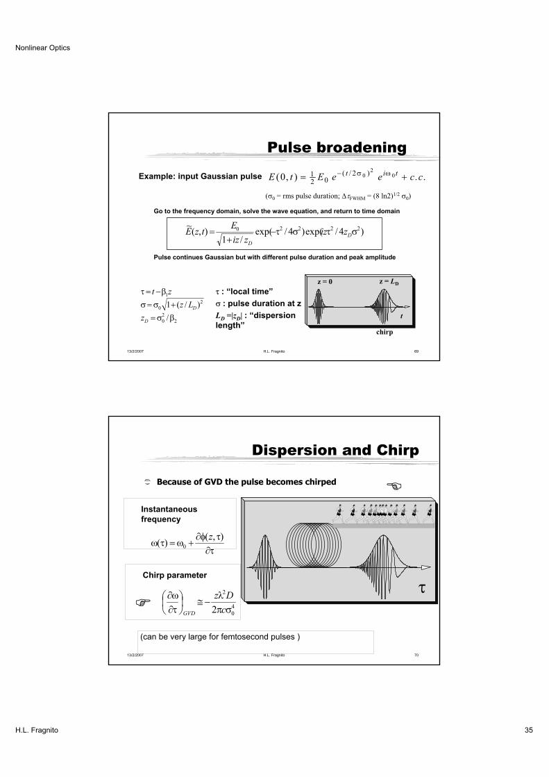
2

2

0

2

0

1

/

)/(1

D

D

z

Lz

zt

Example: input Gaussian pulse

( 0 = rms pulse duration; FWHM = (8 ln2)1/20)

Pulse broadening

t

z = 0 z = LD

chirp

Go to the frequency domain, solve the wave equation, and return to time domain

Pulse continues Gaussian but with different pulse duration and peak amplitude

E t E e e c ct i t( , ) . .( / )0 12 0

2 02

0

)4/exp()4/exp(/1

),(~ 22220

D

D

zizziz

EtzE

: “local time”

: pulse duration at z

LD =|zD| : “dispersion

length”

13/2/2007 H.L. Fragnito 70

Dispersion and Chirp

Because of GVD the pulse becomes chirped

4

0

2

2 c

Dz

GVD

Chirp parameter

Instantaneous

frequency

(can be very large for femtosecond pulses )

),()( 0

z

Nonlinear Optics

H.L. Fragnito 36

13/2/2007 H.L. Fragnito 71

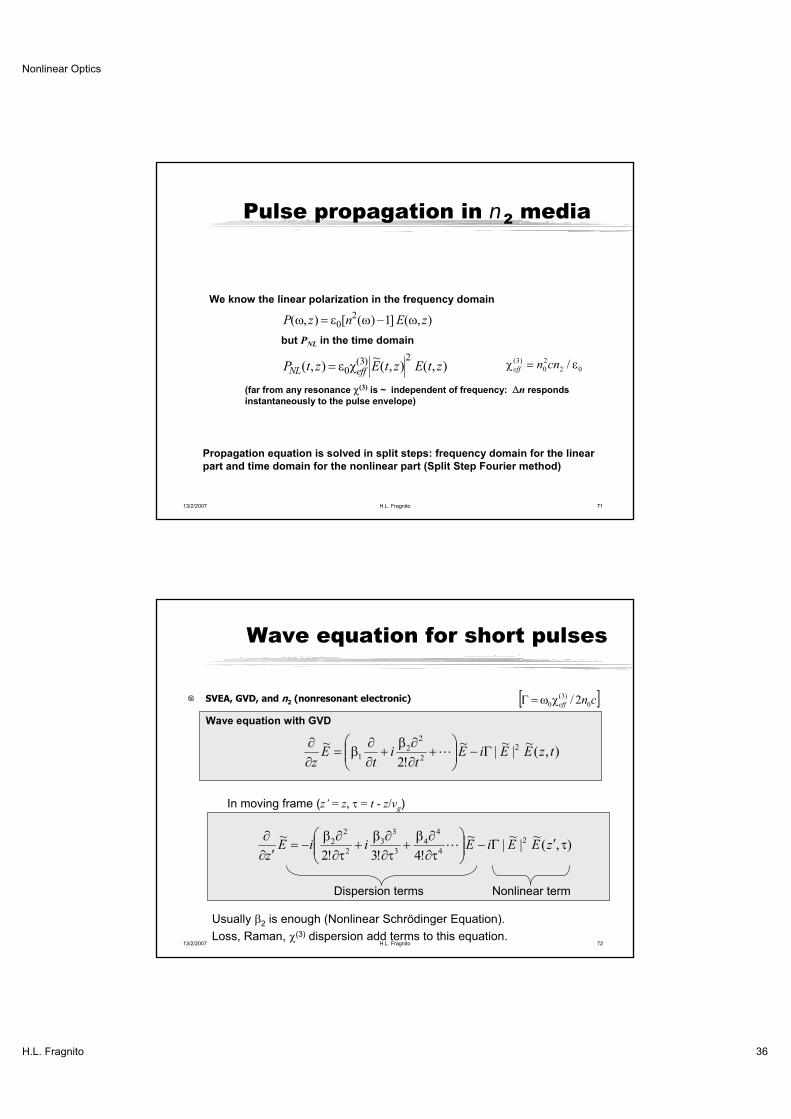
Pulse propagation in n2 media

P z n E z( , ) [ ( ) ] ( , )02 1

We know the linear polarization in the frequency domain

but PNL in the time domain

P t z E t z E t zNL eff( , )~

( , ) ( , )( )0

3 202

2

0

)3( /cnneff

(far from any resonance (3) is ~ independent of frequency: n responds

instantaneously to the pulse envelope)

Propagation equation is solved in split steps: frequency domain for the linear

part and time domain for the nonlinear part (Split Step Fourier method)

13/2/2007 H.L. Fragnito 72

Wave equation for short pulses

SVEA, GVD, and n2 (nonresonant electronic)

Wave equation with GVD

),(~

|~

|~

!2

~ 2

2

2

21 tzEEiE

ti

tE

z

In moving frame (z’ = z, = t - z/vg)

Dispersion terms Nonlinear term

Usually 2 is enough (Nonlinear Schrödinger Equation).

Loss, Raman, (3) dispersion add terms to this equation.

),(~

|~

|~

!4!3!2

~ 2

4

4

4

3

3

3

2

2

2 zEEiEiiEz

cneff 0

)3(

0 2/

Nonlinear Optics

H.L. Fragnito 37

13/2/2007 H.L. Fragnito 73

Self Phase Modulation and Chirp

Region of

Linear Chirp

( )I( )

time,

• Instantaneous frequency of the pulse ( , )zn z

c

I0

0 2

• This gives a ~linear chirp

2

20

ceff

c

SPM cA

Pzn c

• Pulse shape is approximately parabolic near its peak

2

2

21)(

ceff

c

A

PI

(Pc and c: characteristic peak power and duration of light pulse)

13/2/2007 H.L. Fragnito 74

Spectral broadening by SPM

-100 -50 0 50 100

0.0

0.2

0.4

0.6

0.8

1.0

1.2

P0

P0.5

P1

P1.5

P2

P2.5

P3

P3.5

P4

P4.5

P5

SPM on the Spectrum of 70 ps (FWHM) gaussian pulse.

Max Nonlinear phase = 0, 0.5, 1, 1.5, ..., 5

frequency, GHz

Pow

er

density (

10

5)

Initial pulse (z = 0):~

( , ) /E t E e t0 042

02

0 =35 ps

~( , )

~( , ) |

~( , )|E z E ei E z0 0 2

Pulse shape is preserved

but spectrum changes (phase is

a function of time and z):

Spectra as a function of position (z) for fixed input

power, or as a function of power for fixed z.

Maximum nonlinear phase

max E z02

Nonlinear Optics

H.L. Fragnito 38

13/2/2007 H.L. Fragnito 75

Nonlinear Schrödinger equation

Wave equation for dispersive, nonlinear media

Nonlinear Schrödinger Equation (NLSE)

Looks like Schrödinger equation for a particle of mass m in potential V:

Position and time exchanged. If 2 < 0 and n2 > 0then the pulse forms a bounding potential. Pulse

(particle) is trapped in time (space).

iE

z

EE E

~ ~

|~

|~2

22

2 2

it m x

V22

2

-I( )

If 2 < 0 and n2 > 0 (or 2 > 0 and n2 < 0 ) we have “bright solitons”.

If 2 > 0 and n2 > 0 ( 2 < 0 and n2 < 0 ) we can have “dark solitons”.

Neglects third and higher order dispersion

“Eigenstates” of NLSE are solitons.

13/2/2007 H.L. Fragnito 76

Particular cases

Simple solutions of NLSE

1 - Linear case ( = 0)

2 - Purely nonlinear case (no dispersion)

3 - Soliton case

iE

z

EE E z

~ ~

|~

|~

( , )22

2

2 2

Easily solved in frequency domain

~( , )

~( , )E z E e

i z0 2 2

2

Easily solved in time domain

~( , )

~( , ) |

~( , )|E z E e i E z0 0 2

~( , ) / ( / )E c c0 2

2sechIf~

( , )~

( , ) ( / )E z E ei zc0 222then

Nonlinear Optics

H.L. Fragnito 39

13/2/2007 H.L. Fragnito 77

Solitons

Exact cancellation of GVD and SPM chirps

Good side of nonlinearities in communication systems

Occur only in the anomalous dispersion region (D > 0)

after S. Evangelides

4

2

2 cGVD c

Dz

2

20

ceff

c

SPM cA

Pzn

13/2/2007 H.L. Fragnito 78

Soliton stability

Assume an input pulse

• Any reasonable pulse with enoughamplitudebecomes a soliton!!

E Es c( , ) ( ) sech( / )0 1 (| |< 0.5)(which is not a soliton unless = 0)

THEN, if | | < 0.5, the pulse evolves into a soliton!

• The soliton is stable against amplitude variations of ±50%

LD0.0

0.2

0.4

0.6

0.8

1.0Gaussian

time

Soliton

position

• Soliton are (the only) exact, stationary solutions of NLSE

Es c22/

Nonlinear Optics

H.L. Fragnito 40

13/2/2007 H.L. Fragnito 79

Characteristic lengths:

Dispersion length:depends on pulse duration ( c) and dispersion parameter

Nonlinear length:depends on peak pulse intensity and nonlinear parameter

For a given fiber length, L, there are four possibilities:

1) L LD and L LNL : no pulse distortion2) L LD and L LNL : pulse broadens (Dispersive Regime)3) L LD and L LNL : spectral broadening (Nonlinear Regime)4) L LD and L LNL : Soliton Regime

Typical values for optical fibers at = 1.5 µm:

2 = -20 ps2/km, n2 = 3x10-16 cm2/W.

For c = 10 ps and 50 mW peak power in 80 µm2 effective area we have:LD = 5 km and LNL = 12 km

L zD D c| | /| |22

Propagation regimes

L n INL / 2 2

13/2/2007 H.L. Fragnito 80

Further information

Y.R. Shen, The Principles of Nonlinear Optics, Wiley, New York (1984).

R.W. Boyd, Nonlinear Optics, Academic Press, Boston (1992).

P.N. Butcher and D. Cotter, The elements of Nonlinear Optics, Cambridge Univ. Press, Cambridge

(1991).

M. Shubert and B. Wilhelmi, Nonlinear Optics and Quantum Electronics, Wiley, New York (1986).

N. Bloembergen, Nonlinear Optics, Benjamin, Reading, Massachusetts (1965).

D. Marcuse, Principles of Quantum Electronics, Academic Press, New York (1980).

R.H. Pantell and H.E. Putoff, Fundamentals of Quantum Electronics, Wiley, New York (1969).

R. Loudon, The Quantum theory of Light, Oxford Univ. Press, Oxford (1973).

A.E. Siegman, Lasers, University Science Books, Mill Valley (1986).

F.A. Hopf and G.I. Stegeman, Applied Classical Electrodynamics, Wiley, New York (1986).

C. Flytzanis, Theory of nonlinear optical susceptibilities, in Nonlinear Optics, Part A, H. Rabin and

C.L. Tang, eds., Academic Press, New York (1975).

R.L. Sutherland, Handbook of Nonlinear Optics, Marcel Dekker, New York (1996).

G.P. Agrawal, Nonlinear Fiber Optics, Academic Press, San Diego (1989).

E. Iannone, F. Matera, A. Meccozzi, and M. Settembre, Nonlinear Optical Communication Networks, wiley, New York (1998).

G.P. Agrawal, Fiber-Optic Communication Systems, 2nd ed., J. Wiley & Sons, New York (1998).

E. Desurvire, Erbium-doped fiber amplifiers: Principles and applications, Wiley (New York, 1994).

Nonlinear Effects in Optical Fibers and...

Documents

Transcript of Nonlinear Effects in Optical Fibers and...