Nonlinear Dynamics and Statistical Mechanics of Secondary ... · pada protein berdasarkan...

University of Indonesia

Nonlinear Dynamics and StatisticalMechanics of Secondary Protein

Folding

Moch. Januar

0606068442

Faculty of Mathematics and Natural Sciences

Department of Physics

DepokJune 2011

Approval Page

This skripsi is proposed by

Name : Moch. Januar

NPM : 0606068442

Department : Physics

Title : Nonlinear dynamics and statistical mechanics of

secondary protein folding

Has been defended in front of the Examiners Board and accepted as one of

requirements for the degree of Sarjana Sains in Department of Physics, Faculty

of Mathematics and Natural Sciences, University of Indonesia.

Examiners Board

Advisor 1 : Dr. L. T. Handoko (.....................)

Advisor 2 : Dr. Terry Mart (.....................)

Examiner 1 : Dr. Anto Sulaksono (.....................)

Examiner 2 : Dr. Agus Salam (.....................)

Legalized in : Depok, Indonesia

Date : June 1, 2011

iii

And when the prayer has been concluded, disperse within the land and seek

from the bounty of Allah, and remember Allah often that you may succeed.

(Q. S. Al-Jumu’ah 10)

Science is simply common sense at its best.

Thomas Huxley

If it’s green or wriggles, it’s biology.

If it stinks, it’s chemistry.

If it doesn’t work, it’s physics.

Handy Guide to Science

To be a great scientist, there are a lot of sacrifices that have to be made.

Max Planck, in Einstein and Eddington’s Movie

Department of Physics University of Indonesia

Preface

A biophysicist talks physics to the biologists and biology to the

physicists, but then he meets another biophysicist, they just dis-

cuss women.

Anonymous

At one time in the year 2010 (I forget the date and month) in the lab theory,

Andi told me that there is someone who ask him about his skripsi; Ndi, why

is your skripsi mathematics? And then Andi asked me; Why is your skripsi

biology, Jan? We laughed uproariously at that time. We are in Nuclear and

Particle Physics Group but we worked on the outside fields. Nevertheless, I

still use the tools, such as; quantum relativistic, quantum field theory, theory

group, and etc., which are only gotten in the group. I just applied those to

explain the dynamics of bio-matters, such as protein, DNA, and etc. Hopefully

it opens a new breakthrough in research of Theoretical Biophysics, so that the

scientists can treat the cases from the different point of views.

Depok, June 2011

Moch. Januar

Department of Physics i University of Indonesia

Acknowledgments

Praise be to Allah SWT that always provides grace healthy so this Skripsi can

be completed on time. Blessings and greetings may remain devoted to our

master the Prophet Muhammad sallallaahu alaihi wa sallam, to all his friends,

family and his loyal followers until the day of judgement. The authors feel

grateful to Allah SWT for blessing gives an opportunity to the author to have

an education in the Department of Physics University of Indonesia (Fisika UI).

The author would like to thank as much as possible to Dr. L. T. Handoko

for a given behavior pattern, for all the attentions, for the time and opportunity

for questionings, and his patience to the author during this research. He has

introduced and instilled the spirit to be survived in the theoretical physics

environment. He also has guided and funded the author in completing this

Skripsi.

The author feel grateful to Dr. Terry Mart for the conveying lectures and

advices which change the author’s mindset in the study of physics to a more

advanced thinking.

The author also greatly appreciate fruitful discussion with Albert Sulaiman

throughout the work. Author truly grateful to AS for good advices and finan-

cial support in ICMCB 2011 at Malaysia. I can not do anything without his

helps.

I would thank to Dr. Anto Sulaksono, Dr. Agus Salam, Dr. Imam Fachrud-

din, and to all friends (include past) in Lab Teori Fisika UI; Andi O. L., M.

Khalid W., Chrisna S. N., T. P. Djun, Muhandis S., Fathia R. S., Yunita U.,

Fauzi, Saepudin J., Anni, Raditya, Vera, Fahmi M., M. Jauhar, Aziz, and etc.,

for warm hospitality and support during the work and to fill my days like a

real theoretical physicist. Also thanks to my neighbors in Wisma Bhakti Ibu;

Department of Physics ii University of Indonesia

iii

Andrew A., Dani R., Dwiki F., Manggala J., and etc., for all the noisy during

I work. You have tested my diligent to be consistent in my works. and The

more astonishing, my life is colorless without you guys. Besides of that, I

thank to the lecturers and academic staffs who always educate and facilitate

my academic requirements. And do not forget to the fellow soldiers, physics

06; Iyan S., Ryan E., and etc., thank you for the spirit and warmth that were

given for this 5 years.

Beside those peoples who have many important roles in my life, my great

thanks for my parent; Uyuk Syaripudin and Dian Rani, who undeniably give

uncountable meanings in my life, and always support me with immeasurable

patients. And unlimited thank you for Alm. Biyah Sobariyah who has treated

me since childhood. Hopefully she is in the best place in the side of Allah

swt, amin. Do not forget also thanks to my uncle Nasrudin who have always

given advice and funding support for my college and when I was sick. And

also thanks for my lovely brother and sister; Bagas Bintang Samudra, Putri

Zahwa Salsabilla, and Ratu that makes me always have spirit to keep fighting,

since I’m the only one who will be the backbone for them. For Ira Rahmawati,

thanks for the patience of my grumpy face attitude and always take care pa-

tiently when I was sick. Although there are many difficult problems, I will

always make efforts to do my best for you.

The last, author thanks the Group for Theoretical and Computational

Physics LIPI for warm hospitality during the work. This work is partially

funded by the Indonesia Ministry of Research and Technology and the Riset

Kompetitif LIPI in fiscal year 2010 and 2011 under Contract no. 11.04/SK/

KPPI/II/2010 and no. 11.04/SK/KPPI/II/2011 respectively.

The author can not repay to kindness of them. May Allah gives the multiple

replies for all of them.

Depok, June 2011

Moch. Januar


iv

Abstract

A model to describe the mechanism of conformational dynamics in protein

based on matter interactions using lagrangian approach and imposing certain

symmetry breaking is proposed. Both conformation changes of proteins and

the injected non-linear sources are represented by the bosonic lagrangian with

an additional φ4 interaction for the sources. The path integral method is used

to calculate its statistical mechanic properties.

Keywords: protein folding, model, nonlinear, path integral, φ4 interaction

ix+77 pp.; appendices.

References: 32 (1965-2011)

Abstrak

Diajukan sebuah model yang menjelaskan mekanisme pembentukan gerak

pada protein berdasarkan interaksi-interaksi materi dengan menggunakan pen-

dekatan lagrangian dan perusakan simetri. Perubahan bentuk protein dan

sumber non-linier yang disuntikan direpresentasikan oleh lagrangian boson

dengan tambahan interaksi φ4 sebagai sumber gangguan. Metode path in-

tegral digunakan untuk menghitung sifat mekanika statistik-nya.

Kata kunci: pelipatan protein, model, non-linier, path integral, interaksi φ4

ix+77 hlm.; lamp.

Daftar Acuan: 32 (1965-2011)


Contents

Preface i

Acknowledgments ii

Abstract iv

Contents v

List of Figures viii

1 Introduction 1

1.1 Background and Scope of Problem . . . . . . . . . . . . . . . . 1

1.2 Research Aim . . . . . . . . . . . . . . . . . . . . . . . . . . . . 3

1.3 Research Method . . . . . . . . . . . . . . . . . . . . . . . . . . 3

2 Fundamental Concepts 5

2.1 Quantum Field Theory . . . . . . . . . . . . . . . . . . . . . . . 5

2.1.1 U(1) Symmetry . . . . . . . . . . . . . . . . . . . . . . . 6

2.1.2 Spontaneous Symmetry Breaking . . . . . . . . . . . . . 7

2.2 Solitary Wave: Soliton . . . . . . . . . . . . . . . . . . . . . . . 10

2.2.1 Sine-Gordon EOM . . . . . . . . . . . . . . . . . . . . . 10

2.2.2 Nonlinear Klein-Gordon EOM . . . . . . . . . . . . . . . 12

2.3 The Path Integral . . . . . . . . . . . . . . . . . . . . . . . . . . 13

2.4 Functional Derivatives . . . . . . . . . . . . . . . . . . . . . . . 17

2.4.1 Definition . . . . . . . . . . . . . . . . . . . . . . . . . . 17

2.4.2 Miscellaneous Functional Derivative . . . . . . . . . . . . 17

Department of Physics v University of Indonesia

CONTENTS vi

3 Secondary Protein Folding 21

3.1 Global Pictures . . . . . . . . . . . . . . . . . . . . . . . . . . . 21

3.2 Toy Ad-Hoc Model . . . . . . . . . . . . . . . . . . . . . . . . . 22

4 The Models 24

4.1 Linear Conformation Model . . . . . . . . . . . . . . . . . . . . 24

4.1.1 Construction of the Lagrangian . . . . . . . . . . . . . . 24

4.1.2 Symmetry Breaking for the Nonlinear Source . . . . . . . 26

4.1.3 EOMs and its Behaviours . . . . . . . . . . . . . . . . . 28

4.2 Nonlinear Conformation Model . . . . . . . . . . . . . . . . . . 28

4.2.1 Construction of the Lagrangian . . . . . . . . . . . . . . 28

4.2.2 Limit to the Berloff’s Model . . . . . . . . . . . . . . . . 29

4.2.3 Symmetry Breaking for the Both Fields . . . . . . . . . . 30

4.2.4 The EOMs . . . . . . . . . . . . . . . . . . . . . . . . . . 32

5 Numerical Analysis 33

5.1 The Linear Conformation Model . . . . . . . . . . . . . . . . . . 34

5.2 The Nonlinear Conformation Model . . . . . . . . . . . . . . . . 37

6 Statistical Mechanics 39

6.1 The Linear Conformation Model . . . . . . . . . . . . . . . . . . 41

6.1.1 Calculation of the Vacuum Transition Amplitude . . . . 45

6.2 The Nonlinear Conformation Model . . . . . . . . . . . . . . . . 49

7 Results and Discussions 53

7.1 The Numerical Simulations . . . . . . . . . . . . . . . . . . . . . 53

7.2 The Statistical Mechanics Properties . . . . . . . . . . . . . . . 55

8 Conclusion 60

Appendix 61

A Notations 62


CONTENTS vii

B The MATLAB’s Scripts for Solving EOMs of the Model 63

B.1 The Linear Conformation Model . . . . . . . . . . . . . . . . . . 63

B.2 The Nonlinear Conformation Model . . . . . . . . . . . . . . . . 67

C The Maple’s Script for the Statistical Mechanics Calculation 71

C.1 Heat Capacity v.s Temperature: The Both Conformational Mod-

els . . . . . . . . . . . . . . . . . . . . . . . . . . . . . . . . . . 71

C.2 Heat Capacity v.s Temperature: Quantum Fluctuation Varia-

tions in the Linear Conformational Models . . . . . . . . . . . . 72

C.3 Heat Capacity v.s Temperature: Quantum Fluctuation Varia-

tions in the Nonlinear Conformational Models . . . . . . . . . . 73

References 74


List of Figures

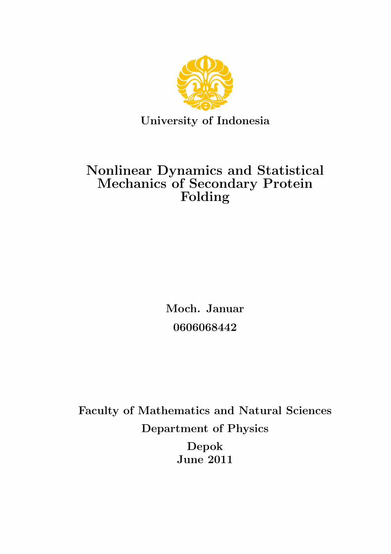
2.1 Potential V (φ) = 12µ2φ2 + 1

4λφ4 with λ > 0 for (a) µ2 > 0 and

(b) µ2 < 0. . . . . . . . . . . . . . . . . . . . . . . . . . . . . . . 9

3.1 (Color online.) Time snapshots of the secondary folding of a

toy protein consisting of five regions where the local potential

energy functional is constant with γ1 = γ5 = 0.9, γ2 = γ4 =

0.1, and γ3 = 0.55. The regions with different values of assigned

γi are shown in different colours (shadings) along the initial (t

= 0) state. Initially the solitary wave is ψ(t = 0) = 2sech[2(x−40)]exp[i(x − 40)] and φ = 0. The coefficients in (6)(8) are

ζ = 0.1,Γ = 0.1,m = 0.5, C = 2,Λ = 0.5. The position of

the solitary wave is shown in green (light Grey) and the arrows

indicate the direction of its motion. . . . . . . . . . . . . . . . . 22

5.1 The discretized grid for solving the EOMs over the coordinate

space R. . . . . . . . . . . . . . . . . . . . . . . . . . . . . . . . 34

7.1 The soliton propagations and conformational changes on the

protein backbone inducing protein folding. The vertical axis in

soliton evolution denotes time in second, while the horizontal

axis denotes its amplitude. The conformational changes are on

the (x, y, z) plane. The constants of the simulation are chosen as

m = 0.08 eV ≡ 1.42× 10−37 kg, L = 12 eV −1 ≡ 2, 364 nm,Λ =

2.83× 10−3, λ = 3× 10−3, and ~ = c = 1. . . . . . . . . . . . . . 54

Department of Physics viii University of Indonesia

LIST OF FIGURES ix

7.2 The soliton propagations and conformational changes on the

protein backbone inducing protein folding. The vertical axis in

soliton evolution denotes time in second, while the horizontal

axis denotes its amplitude. The conformational changes are on

the (x, y, z) plane. The constants of the simulation are chosen as

m = 0.008 eV ≡ 1.42×10−38 kg, L = 12 eV −1 ≡ 2, 364 nm,Λ =

2.83× 10−3, λψ = 5× 10−3, λφ = 6× 10−3, and ~ = c = 1. . . . . 55

7.3 Heat capacity v.s temperature, comparing the both conforma-

tional model. . . . . . . . . . . . . . . . . . . . . . . . . . . . . 58

7.4 Heat capacity v.s temperature with quantum fluctuation term

variations N = 1

4π sinh( kβ2), where (a) linear conformation model

and (b) nonlinear conformational model. . . . . . . . . . . . . . 59


Chapter 1

Introduction

Has there (not) come upon man a period of time when he was not

a thing (even) mentioned?

Indeed, We created man from a sperm-drop mixture that We may

try him; and We made him hearing and seeing.

(Q. S. Al-Insan 1-2)

1.1 Background and Scope of Problem

Did you know about protein? Protein is a macro molecule that has essential

role for living things. Organisms need protein in almost of all its activities. For

example, the protein acts as a hormone that transmits information between

cells and organs, serves as a defense against infections, controls the expression

of genes, forms a large molecular organelles such as ribosome, and many other

activities. Moreover, even the protective layer of a virus is also protein. In

other words, every living organism cannot be separated from the protein [1].

To understand biological processes of an organism, the sequence of proteins

must be known. From protein bio-synthesis, the pathway of proteins are de-

termined by the sequences of its amino acid constituents, and this prediction

has been known as the protein folding problem [2].

The research about protein folding mechanism is very important. It is

known that the protein mis-folding has been identified as the main cause of

several diseases like cancers and so on [3]. The mis-folding proteins cannot

Department of Physics 1 University of Indonesia

1.1. BACKGROUND AND SCOPE OF PROBLEM 2

function essentially in biological processes, or in other words, these proteins are

broken. It will accumulate and form a new species which are toxic. Then can

lead to genetic mutations, weakening of the immune system and also can cause

many kind of diseases. The diseases that are caused by protein folding faulty

have been classified in a group that was called Protein Conformational Disor-

ders (PCDs). The various kinds of diseases in PCDs are including Alzheimer’s

disease (AD), haemolytic anemia, transmissible spongiform encephalopathies

(TSEs), serpin-deficiency disorders, Huntington’s disease (HD), cystic fibro-

sis, diabetes type II, amyotrophic lateral sclerosis (ALS), Parkinson’s disease

(PD), dialysis-related amyloidosis and more than 15 other diseases including

cancers [4].

Unfortunately, our understanding on the underlying folding mechanism

has not been at the satisfactory level. The main mechanism responsible for a

structured folding pathway have not yet been identified at all. These lead the

protein folding problem becomes one of the most important issues of modern

science [2].

Seeing the above-mentioned importance cases, various models of the dy-

namics of protein folding have been made. Many approaches are done to de-

scribe the protein folding phenomenon. Recently, a toy model of protein folding

that mediated by soliton has been proposed [5]. Further, Mingaleev et.al. have

shown that the nonlinear excitations play an important role in conformational

dynamics by decreasing the effective bending rigidity of a biopolymer chain

leading to a buckling instability of the chain [6]. Following this understanding,

a model to explain the transition of a protein from a metastable to its ground

conformation induced by solitons has been proposed [7]. In the model the

mediator of protein transition is the Davydov solitons propagating through

the protein backbone. Moreover, using analogous style with the mentioned

models, a lot of nonlinear models of DNA have been developed [8, 9].

At present, the most reliable theoretical explanation for this kind of the

conformational dynamics of biomolecules is the so-called ab initio quantum

chemistry approach. This however requires astronomical computational power

to deal with realistic biological systems [10, 11]. In contrary, there are some


1.2. RESEARCH AIM 3

phenomenological model describing the folding pathway as a result of the in-

terplay between the energy transfer from a solitary solution that travels along

the protein backbone and string tension [12].

This work follows the later approach, but starting from the first principle

using the lagrangian method to derive the responsible interactions and to clar-

ify its origins. The folding pathway is modeled as consequence of existence of

nonlinear sources (soliton) which are induced into the protein backbone. All

the interactions among the nonlinear sources and protein backbone would be

modeled by φ4 self-interactions. Furthermore, its statistical mechanics prop-

erties would be obtained using path integral method [13]. The semi-classical

expansions will be used in order to separate between the classical and quantum

aspects of the fields [14].

Investigating the dynamical of protein folding hopefully can obtain knowl-

edges which have good contribution to the health of the common society.

1.2 Research Aim

This research has main aim to review the nonlinear dynamics of secondary

protein structure. This work is modeling the conformational changes of the

backbone which leads transition process of protein from the unfolded state

which looks like string into the secondary folded form which looks like a spiral

(alpha helix). To support the model, its statistical mechanics properties would

be shown by using path integral approach.

1.3 Research Method

This research is theoretics based on Lagrangian formulation [15]. The la-

grangian is used to represent all the responsible interactions which is predicted

by this model, and then certain symmetry breaking will be involved.

In the model, the involved interactions are imposing nonlinear terms that

would produce nonlinear equation of motions (EOMs). So that, it is more

convenient to solve it numerically using forward finite difference method [16,


1.3. RESEARCH METHOD 4

17]. The numerical simulation will be obtained with the help of computational

softwares, that is; MATLAB and Maple.

Furthermore, path integral method will be used in order to calculate the

partition function of the system. This attempt is important to find statistical

mechanics properties of occurred interactions in the folding process [18, 19].


Chapter 2

Fundamental Concepts

”You cannot teach a man anything; you can only help him find it

within himself.”

Galileo Galilei

2.1 Quantum Field Theory

Quantum field theory is a unification of special relativity and quantum me-

chanics. This theory formed the framework of the standard model in particle

physics [15]. Mathematical foundation in quantum field theory is the formula-

tion of lagrangian. One can observe a system by looking from its lagrangian.

Afterwards, by using Euler-Lagrange equation, the relevant equation of motion

of the system can be obtained. And many more works can be done from the

lagrangian.

It will be cleared by considering properties of the lagrangian deeply. If the

field φ(x) has a kinetic energy T and the potential V, then lagrangian is

L = T − V . (2.1)

In the continuous case, actually it should be worked by using density of the

lagrangian LL = T − V =

∫d3xL . (2.2)

Integration the lagrangian over the time gives a new important quantity


2.1. QUANTUM FIELD THEORY 6

namely action S

S =

∫dtL . (2.3)

Action is functional because the action always takes functions as arguments

and produces a number. Particles always take the path with the smallest

action. To find the path, then the variation of the action should be minimized.

This is done by describing the action as the minimum term and a variation

term.

S −→ S + δS . (2.4)

The action is minimum if satisfied

δS = 0 . (2.5)

In quantum field theory, lagrangian density is used more often, then the

equation for the action will be written as

S =

∫d4x L . (2.6)

For the sake of abbreviation, the lagrangian density L is often called just

Lagrangian.

This is an example of a lagrangian for a free scalar particle

L =1

2(∂µφ)(∂µφ)− 1

2m2φ2 . (2.7)

The first term is the kinetic energy (containing (∂φ)2) and the second one is

the mass term of the field (containing φ2).

2.1.1 U(1) Symmetry

In quantum field theory, one learned that any theory is built on a certain

symmetry. The theory must be invariant against the transformation of gauge

global and local levels of symmetry are built. If the theory is invariant, then

all the produced physical quantities have value which does not depend on the

inertial reference frame where it was measured.



The above statement implies that the lagrangian which is made in a theory

must be invariant to a certain symmetry. In field theory, global and local it

gauge symmetry are often used to build a model. Global gauge transformation

has form

φ→ eiθφ, (2.8)

where θ is constant.

Meanwhile local gauge has form

φ→ eiα(x)φ, (2.9)

where α(x) is a space-time function.

To see the invariance of the two transformations above, consider the fol-

lowing lagrangian

L =1

2(∂µφ)(∂µφ)− 1

2m2φ2 . (2.10)

It was clear that the above lagrangian invariant against global transformation

but not for local transformation. First term of the lagrangian is not invariant

to local gauge transformation. To make the lagrangian invariant, the derivative

operator ∂µ must be modified become covariant derivative Dµ and a new gauge

field should be introduced.

Unfortunately, the author wont explain this symmetry problem further,

since it did not relevant to the our model. More details explanation can be

seen in [15].

2.1.2 Spontaneous Symmetry Breaking

One of more interesting idea in quantum field theory is symmetry breaking.

This concept can be related to the parity symmetry [15, 20]. Consider the

lagrangian as follow

L ≡ T − V =1

2(∂φ)2 − (

1

2µ2φ2 +

1

4λφ4) , (2.11)



with λ > 0. The lagrangian is invariant to the parity transformation φ to −φ.

to describe scalar field with mass µ. The φ4-term represents self-interaction of

the field with a coupling constant λ.

The two possible potential has been shown in Fig. (2.1). The left figure (a)

for µ2 > 0 Ground state (vacuum) is λ = 0. This state obeys parity symmetry

of the lagrangian. Meanwhile, the more interesting case is located in the right

side (b) for µ2 < 0. Now, the lagrangian in Eq. (2.11) has a mass term with

the wrong sign for the field φ, as a sign of the relative term φ2 by the kinetic

energy T is a positive (it is should be negative). Unlike the case of (a), in case

(b) the potential has two minimum values.

These minimum values satisfy

∂V

∂φ= φ(µ2 + λφ2) = 0 (2.12)

and is located on

φ = ±ν with ν =

√−µ2

λ(2.13)

Extreme value of φ = 0 is not a state with minimum energy. φ = 0 is an

unstable situation (see Figure 2.1), the situation can be shifted to one of two

other minimum conditions, where φ = +ν or φ = −ν, which are the actual

ground states. However, choosing one of these conditions would break the

symmetry.

In the case of lagrangian (2.11), note that the actual minimum is at φ = ±ν.

The value φ = 0 is not stable, then the perturbation expansion of this point is

not convergent. Thus, perturbation expansion must be made to the φ = +ν

or φ = −ν. So that, φ(x) can be written as,

φ(x) = ν + η(x), (2.14)

with η(x) represents the quantum fluctuations to a minimum. In this case,

φ = +ν is chosen, but it wont lost its generality, since the φ = −ν can



Figure 2.1: Potential V (φ) = 12µ2φ2 + 1

4λφ4 with λ > 0 for (a) µ2 > 0 and (b)

µ2 < 0.

always be generated from the reflection symmetry. Substitution (2.14) into

the lagrangian (2.11) obtains,

L′ = 1

2(∂η)2 − λν2η2 − λνη3 +

1

4λη4 + const. (2.15)

Field η has a mass term with the correct sign because the sign of the η2

relative to the kinetic energy is negative. Comparing the first two terms in the

lagrangian (2.7) will obtained,

mη =√

2λν2 =√−2µ2. (2.16)

Meanwhile, the higher order of η represents its self-interaction.

There is confusion here. Lagrangian L of the Eq. (2.11) and L′ the Eq.

(2.15) are equivalent. The transformation (2.14) is not possible to change the

physical meaning. If the two Lagrangian can be solved exactly, they should

produce identical physics. But in particle physics, the exact calculation is

difficult, instead perturbation theory is usually used and the fluctuations is

calculated around the minimum energy. If L is used, perturbation series will

not converge as the expansion is around the unstable point φ = 0. So using


2.2. SOLITARY WAVE: SOLITON 10

L′ and the expansion is done in η in the vicinity of the stable point φ =

+ν. In perturbation theory, L′ give a true picture of physics, while L is not.

Thus, scalar particles (described by the Lagrangian L and L′ are equivalent in

principle) should be had a mass.

This method is often called ”spontaneous symmetry breaking. ” In theory

version of the L′, the reflection symmetry of the Lagrangian has been damaged

with a choice of ground state φ = +ν (instead of φ = −ν). Often, this method

is used to ”arouse the mass” of a field.

2.2 Solitary Wave: Soliton

Besides of the quantum field theory and its symmetry, this work will obey

some properties of soliton. The interactions are represented by bosonic φ4-

interaction and Sine-Gordon potential which, of course, will produce sequences

of nonlinear equation of motions. Its solutions can be approached using trav-

eling solution. This solution benefits one of the properties of solitary wave

(soliton).

In this section, some examples of finding the traveling solution of a non-

linear PDE can be explained briefly. It use some analogies with the Korteweg

and deVries (KdV) method [21, 22].

2.2.1 Sine-Gordon EOM

Taking into consideration the Sine-Gordon equation of motion (EOM) as fol-

lows,

�φ+1

bsin(bφ) = 0

φtt − φxx +1

bsin(bφ) = 0 , (2.17)

where b is an arbitrary constant. To have a traveling solution, the two di-

mensional space and time coordinates should be reduced into one degree of



freedom with certain velocity,

φ(x, t) = φ(x− vt) = φ(z) . (2.18)

Then the derivatives can be written as,

φt =∂φ

∂z

∂z

∂t= −vφz , (2.19)

φtt = v2φzz, and φxx = φzz . (2.20)

Thus, the PDE in Eq. (2.17) is changed into an ODE,

(v2 − 1)φzz +1

bsin(bφ) = 0 . (2.21)

Assume (v2 − 1) = a for abbreviation the notation, and then times the

equation with φz,

aφzzφz +1

bsin(bφ)φz = 0

a

2

dφ2z

dz− 1

b2d

dz(cos(bφ)) = 0

d

dz

(a

2φ2z −

1

b2cos(bφ)

)= 0 . (2.22)

By integrating the last above equation in term of z, and assuming limx→0 φ = 0

to vanish the integral constants, thus obtains,

a

2φ2z =

1

b2cos(bφ)

dφ

dz=

√2

ab2cos(bφ)∫

dφ√cos(bφ)

=

√2

ab2

∫dz . (2.23)

(2.24)

The left side integral can be solved by utilizing properties of the elliptic integral

[23] from 0 to φ0, and the right one can be integrated directly from 0 to z. By

integrating the both side integrals and inverting, the traveling solution for the



Sine-Gordon is obtained as [15],

φ(x− vt) =4

barctan

(exp[±(

γ√b(x− vt)]

), (2.25)

where γ = (1 − v2)− 12 . The positive sign in the solution is called kink soliton

and the negative one is called antikink soliton.

2.2.2 Nonlinear Klein-Gordon EOM

Supposing the Sine-Gordon EOM in Eq. (2.17) has infinitesimal b, such that

it can be expanded using Taylor’s expansion up to second order.

�φ+1

b

(bφ− (bφ)3

3!

)= 0

φtt − φxx + φ− b2

3!φ3 = 0 , (2.26)

It is arrived to the massive nonlinear Klein-Gordon EOMs as follows [15],

φtt − φxx +m2φ− λ

3!φ3 = 0 . (2.27)

where m stands for unit mass which is put by hand and λ = b2 for the self-

interaction coupling. Although the NKG equation can be derived form the

Sine-Gordon equation, but it does not mean that both have the same solution.

Nevertheless, the NKG also can be solve by using traveling solution method,

same as above.

In the traveling solution scheme, same as before, the PDE in Eq. (2.27)

should be changed into an ODE,

aφzz +m2φ− λ

3!φ3 = 0 . (2.28)

where a = (v2 − 1). Using same mathematical tricks as earlier by timing the

equation with φz and assuming limx→0 φ = 0 to vanish the integral constants,

obtains

aφzφzz +m2φzφ−λ

3!φzφ

3 = 0


2.3. THE PATH INTEGRAL 13

a

2

dφ2z

dz+m2

2

dφ2

dz− λ

4!

dφ4

dz= 0

d

dz

(a

2φ2z +

m2

2φ2 − λ

4!φ4

)= 0

a

2φ2z +

m2

2φ2 − λ

4!φ4 = 0

−m2

aφ2 +

2λ

a4!φ4 = φ2

z√−m

2

aφ2 +

2λ

a4!φ4 =

dφ

dz∫1√

2λ4!φ4 −m2φ2

dφ =

√1

a

∫dz . (2.29)

Same as before, by utilizing the elliptic integral method, the soliton solution

for the NKG equation can be obtained as follow,

φ(x− vt) = ± m√λ

tanh(m√

2(x− vt)) . (2.30)

Therefore, solitary wave solution for the Sine-Gordon and NKG equations

can be investigated easily using this traveling approximation.

2.3 The Path Integral

The statistical mechanics for the models will be calculated using path integral

method. At least, a brief introduction to the path integral calculation should

be given as one of the preliminary requisites.

The calculation will be started from Huygen’s Principles [15]

ψ(qf , tf ) =

∫K(qf tf , qiti)ψ(qi, ti)dqi . (2.31)

The probability that is observed at qf at time tf is

P (qf tf ; qiti) = |K(qf tf ; qiti)|2 . (2.32)

Take as consideration the relation of eigenstate between Schrodinger picture



=1

2π~

∫dpeip(qj+1−qj)/~ − iτ

~〈qj+1|H|qj〉 . (2.42)

For special case, supposing a system with Hamiltonian as follow

H =p2

2µ+ V (q) , (2.43)

then the path integral calculation becomes

〈qj+1|H|qj〉 = 〈qj+1|p2

2µ|qj〉+ 〈qj+1|V (q)|qj〉

〈qj+1|p2

2µ|qj〉 =

∫dp′dp〈qj+1|p′〉〈p′|

p2

2µ|p〉〈p|qj〉 . (2.44)

It is familiar to know that 〈qj+1|p′〉 = (2π~)−1/2eip′qj+1/~, then

〈qj+1|p′

2µ|qj〉 =

∫dp′dp

2π~eip′qj+1/~e−ipqj/~〈p′| p

2

2µ|p〉

=

∫dp′dp

2π~ei/~(p

′qj+1−pqj) p2

2µδ(p′ − p)

=1

2π~

∫dpe

ip~ (qj+1−qj) p

2

2µ

=

∫dp

hexp

[ip

~(qj+1 − qj)

]p2

2µ. (2.45)

Assuming the potential is local, then

〈qj+1|V (q)|qj〉 = V

(qj+1 + qj

2

)〈qj+1|qj〉

= V (qj+1 + qj

2)δ(qj+1 − qj)

= V ((qj+1 + qj)

2)

∫dp

hexp

[1

~p(qj+1 − qj)

]. (2.46)

For abbreviation the notation, suppose

qj =qj+1 + qj

2, (2.47)

〈qj+1|V (q)|qj〉 = V (q)

∫dp

hexp

(ip

~(qj+1 − qj)

), (2.48)

〈qj+1|H|qj〉 =

∫dp

hexp

[(ip

~(qj+1 − qj)

](p2

2µ+ Vq

), (2.49)



=

∫dp

hexp

[ip

~(qj+1 − qj)

]H . (2.50)

So that,

〈qj+1tj+1|qjtj〉 =

∫dpjh

exp

[ip

~(qj+1 − qj)

](1− iτ

~H

)(2.51)

=

∫dpjh

exp

[ip

~(qj+1 − qj)

]exp

(−i~τH

)(2.52)

=

∫dpjh

exp

[i

~pj(qj+1 − qj)− τH)

], (2.53)

where pj is the momentum between tj and tj+1.

Therefore, the full propagator can be written as

〈qf tf |qiti〉 = limn→∞

∫ n∏j=1

dqj

n∏j=0

dpjexp

{i

~

n∑j=0

[pj(qj+1 − qj)

− τH(p, q)]} . (2.54)

There is another form for the transition amplitude, which holds when H is of

the form Eq. (2.43), since in that case we can perform the p-integration. The

above equation becomes,

〈qf tf |qiti〉 = limn→∞

∫ n∏1

dqj

n∏0

dpj~

exp

{i

~

n∑j=0

[pj(qj+1 − qj)τ

−p2j2µ− V (qj)τ

]}= lim

n→∞

( µ

ihτ

)(n+1)/2∫ n∏

1

dqj

×exp

{iτ

~

n∑j=0

[µ

2

(qj+1 − qj

τ

)2

− V

]}. (2.55)

In symbolic form it can be written as,

〈qf tf |qiti〉 = N

∫Dqexp

[i

~

∫ tf

ti

L(q, q)dt

]. (2.56)

The last equation will be used in partition function calculation later.


2.4. FUNCTIONAL DERIVATIVES 17

2.4 Functional Derivatives

2.4.1 Definition

Functional derivative method is very useful to outsmart the interaction terms in

path integral calculation for the partition function. In this trick, the nonlinear

fields and the interaction term in the lagrangian will be changed into functional

derivative operators, then the partition function becomes linear and can be

solved by plane wave approach. It will be clear in Chapter 6. In this section,

the definition and some example about functional derivative will be discussed.

In this case, the functional derivative means derivative of a functional in-

tegral. A functional integral is denoted by F [f(x)] and it is usually called just

functional. Derivative of the functional is defined by analogy with ordinary

derivative [15], that is

δF [f(x)]

δf(y)= lim

ε→0

F [f(x) + εδ(x− y)]− F [f(x)]

ε. (2.57)

All of its properties are analogous with the ordinary derivatives.

2.4.2 Miscellaneous Functional Derivative

Some kind of functional derivatives that perhaps useful in path integral calcu-

lation will given.

Identity Functional

Considering the functional

F [f ] =

∫f(x)dx , (2.58)

then derivative of the functional is

δF [f ]

δf(x)= lim

ε→0

∫(f(x) + εδ(x− y))dx−

∫f(x)dx

ε

= limε→0

∫f(x)dx+

∫εδ(x− y)dx−

∫f(x)dx

ε



=

∫δ(x− y)dx

= 1 . (2.59)

Parameter Function

Supposing Fx[f ] =∫G(x, y)f(y)dy, where x in the left side is only a parame-

ter. Then the derivative is

δFx[f ]

δf(z)= lim

ε→0

∫G(x, y)(f(y) + εδ(y − z))dy −

∫G(x, y)f(y)dy

ε

= limε→0

∫G(x, y)f(y)dy +

∫εG(x, y)δ(y − z)dy −

∫G(x, y)f(y)dy

ε

=

∫G(x, y)δ(y − z)dy

= G(x, z) . (2.60)

Product

Supposing F [f ] =∫A[f(x)]B(f(x)dx. Then

δF [f ]

δf(y)= lim

ε→0

F [f(x) + εδ(x− y)]− F [f(x)]

ε

= limε→0

1

ε

{∫(A[f(x) + εδ(x− y)]B[f(x) + εδ(x− y)]) dx

−∫A[f(x)]B[f(x)]dx

}= lim

ε→0

1

ε

{∫(A[f(x) + εδ(x− y)]B[f(x) + εδ(x− y)]

−A[f(x) + εδ(x− y)]B[f(x)] + A[f(x) + εδ(x− y)]B[f(x)]

−A[f(x)]B[f(x)]) dx}

= limε→0

∫A[f(x) + εδ(x− y)]

((B[f(x) + εδ(x− y)]−B[f(x)]

ε

)dx

+

∫ (A[f(x) + εδ(x− y)]− A[f(x)]

ε

)B[f(x)]dx

=

∫limε→0

A[f(x) + εδ(x− y)] limε→0

((B[f(x) + εδ(x− y)]−B[f(x)]

ε

)dx

+

∫limε→0

(A[f(x) + εδ(x− y)]− A[f(x)]

ε

)B[f(x)]dx



=

∫A[f(x)]

δB[f(x)]

δf(y)dx+

∫δA[f(x)]

δf(y)B[f(x)]dx . (2.61)

Therefore, we have product rule of functional derivative

δF [f(x)]

δf(y)=

∫A[f(x)]

δB[f(x)]

δf(y)dx+

∫δA[f(x)]

δf(y)B[f(x)]dx . (2.62)

Quotient

Considering F [f)] =∫ A[f(x)]

B(f(x)dx. Then

δF [f ]

δf(y)= lim

ε→0

F [f(x) + εδ(x− y)]− F [f(x)]

ε

= limε→0

1

ε

{∫ (A[f(x) + εδ(x− y)]

B[f(x) + εδ(x− y)]

)dx−

∫A[f(x)]

B[f(x)]dx

}= lim

ε→0

1

ε

{∫A[f(x) + εδ(x− y)]B[f(x)]

B[f(x) + εδ(x− y)]B[f(x)]dx

−∫

B[f(x) + εδ(x− y)]A[f(x)]


}= lim

ε→0

1

ε

{∫A[f(x) + εδ(x− y)]B[f(x)]− A[f(x)]B[f(x)]


+

∫A[f(x)]B[f(x)]−B[f(x) + εδ(x− y)]A[f(x)]


}=

∫ {(limε→0

(A[f(x) + εδ(x− y)]− A[f(x)])

εB[f(x)]

−A[f(x)] limε→0

(B[f(x) + εδ(x− y)]−B[f(x)])

ε

)× lim

ε→0

1

B[f(x) + εδ(x− y)]B[f(x)]

}dx

=

∫ δA[f(x)]δf(y)

B[f(x)]− A[f(x)] δB[f(x)]δf(y)

B[f(x)]B[f(x)]dx . (2.63)

Therefore, the quotient rule of functional derivative has been obtained as

δF [f ]

δf(y)=

∫ δA[f(x)]δf(y)

B[f(x)]− A[f(x)] δB[f(x)]δf(y)

B[f(x)]B[f(x)]dx . (2.64)



Exponential

Solving the derivative of exponential functional is most important. It appears

frequently in a lot of path integral cases. Let F [f)] = e∫G(x,y)f(x)dx.

δF [f ]

δf(z)= lim

ε→0

e∫G(x,y)(f(x)+εδ(x−z))dx − e

∫G(x,y)f(x)dx

ε

= limε→0

e∫G(x,y)f(x)dxe

∫εG(x,y)δ(x−z)dx − e

∫G(x,y)f(x)dx

ε

= limε→0

e∫G(x,y)f(x)dx

(e∫εG(x,y)δ(x−z)dx − 1

)ε

, (2.65)

e∫εδ(x−z)dx can be expanded using Taylor’s expansion. Because of ε is very

small, this expansion can be approached only first two terms.

e∫εG(x,y)δ(x−z)dx ≈ 1 +

∫εG(x, y)δ(x− z)dx . (2.66)

Therefore, the derivative becomes

δF [f ]

δf(z)= lim

ε→0

e∫G(x,y)f(x)dx

(1 +

∫εG(x, y)δ(x− z)dx− 1

)ε

= e∫G(x,y)f(x)dx

∫G(x, y)δ(x− z)dx

= e∫G(x,y)f(x)dxG(z, y) . (2.67)

Then, the exponential functional derivative is

δF [f ]

δf(z)= G(z, y)e

∫G(x,y)f(x)dx . (2.68)

Hopefully this derivation will help calculations in this work.


Chapter 3

Secondary Protein Folding

Recite in the name of your Lord who created -

Created man from a clinging substance.

(Q.S. Al-’Alaq 1-2)

3.1 Global Pictures

The protein folding problem is a prediction of the structure of proteins from

the knowledge of their amino acid sequences. There are many stages structure

of protein, namely primary structure, secondary and so on, depend on how its

amino acids are composed.

The primary is a state when the protein constituent amino acids which

held together by covalent or peptide bonds. The amino acids did not interact

with each other, so that the protein looks like a string.

Meanwhile, the secondary structure consists of the shape representing each

segment of a polypeptide tied by hydrogen bonds, Van Der Walls forces, elec-

trostatic interaction and hydrophobic effects [24]. It is moreover formed around

a group of amino acids considered as the ground state. Then it is extended

to include adjacent amino acids till the blocking amino acids are reached, and

the whole protein chain along the polypeptide adopted its preferred secondary

structure. The famous secondary protein structures are alpha helix and beta

sheet.

The amino acids which are assembling the protein sequences change the


3.2. TOY AD-HOC MODEL 22

Figure 3.1: (Color online.) Time snapshots of the secondary folding of a toyprotein consisting of five regions where the local potential energy functionalis constant with γ1 = γ5 = 0.9, γ2 = γ4 = 0.1, and γ3 = 0.55. The regionswith different values of assigned γi are shown in different colours (shadings)along the initial (t = 0) state. Initially the solitary wave is ψ(t = 0) =2sech[2(x − 40)]exp[i(x − 40)] and φ = 0. The coefficients in (6)(8) are ζ =0.1,Γ = 0.1,m = 0.5, C = 2,Λ = 0.5. The position of the solitary waveis shown in green (light Grey) and the arrows indicate the direction of itsmotion.

protein shape from the primary to the secondary and subsequent structures.

Some models have then been proposed to explain such protein transition [5, 7,

10, 11, 12, 25, 26, 27]. This work is also modeling conformational dynamics of

secondary structure of protein.

3.2 Toy Ad-Hoc Model

This work actually reproduces toy ad-hoc model which has been made by

Berloff [12]. In this section, the toy model will be described briefly.

The model produces such nonlinear equations of motion by defining the

lagrangian as follow,

L = iψ∗∂tψ−|∂xψ|2+|ψ|4+1

2m(∂tφ)2−V (φ)−U(|ψ|, φ)−T (φ)−|∂xφ|2 (3.1)

The first three terms are the lagrangian of nonlinear Schrodinger equation,

while U is the potential interaction between solitons with protein backbone,

V describes the local potential that represents the shape of the body proteins,


3.2. TOY AD-HOC MODEL 23

and T is the strain potential between the peptide building blocks of protein.

Those potentials are written as follows,

U(|ψ|, φ) = Λ|ψ|2(φ− 12)2 ,

V (φ) = C (φ− γ(x))2 (γ(x)2 + +2γ(x)(φ− 1) + φ(3φ− 4)) ,

T (φ(x)) = η [(φ(x)− φ(x− li))2 + (φ(x)− φ(x+ li))2]

(3.2)

By using Euler-Lagrange equation, one can obtain two coupled nonlinear

EOMs as follows,

i∂tψ = −ψxx +

[Λ(φ− 1

2)2 − 2|ψ|2

]ψ , (3.3)

m∂ttφ = −12Cφ(φ− 1)(φ− γ(x))− 2Λ|ψ|2(φ− 1

2) + φxx

−2ζ(φ− φ(x− li))− 2ζ(φ− φ(x+ li))− Γ∂tφ . (3.4)

The strain potential term T in the above EOMs has been ignored for the sake

of simplicity.

Berloff was succeed reproduce nonlinear EOMs which can describe the non-

linear dynamics of secondary protein folding. As can be seen in Fig. (3.1), the

numerical result of the EOMs shows either how a protein chain can fold from

primary to the secondary forms. Nevertheless, the model is not built from first

principle. The interaction terms are adding just put by hand.


Chapter 4

The Models

Our imagination is stretched to the utmost, not, as in fiction, to

imagine things which are not really there, but just to comprehend

those things which ’are’ there.

Richard Feynman

This chapter is the core of my work. The first principle models of secondary

protein folding will be constructed with two approximations, namely linear

conformation and nonlinear conformation [28, 29]. The difference of the both

approaches are only in the initial stage assumptions, that is linear and nonlin-

ear initial protein backbone forms.

4.1 Linear Conformation Model

4.1.1 Construction of the Lagrangian

The model is an extension of the toy model proposed in [5]. More than consid-

ering a self-interaction mechanism as proposed in [5] and subsequently devel-

oped in [7, 12], more realistic model is introduced. In this model, the dynamics

of amino acids forming proteins is initially considered as a free and linear sys-

tem of bosonic matters. Further, external nonlinear sources, like laser or light

bunch, are introduced. The sources which propagate through the protein back-

bone interact each other with the amino acids to induce conformation changes.


4.1. LINEAR CONFORMATION MODEL 25

The model describes the conformation changes as the dynamics of amino

acids using a free and massive (relativistic) bosonic lagrangian as below,

Lc =1

2(∂µφ)† (∂µφ) +

1

2m2φφ†φ , (4.1)

where φ represents the conformation field and φ† ≡ (φ∗)T is the hermitian

conjugate for a general complex field φ. On the other hand, the nonlinear

sources represented by the field ψ are also governed by a massless bosonic

lagrangian,

Ls =1

2(∂µψ)† (∂µψ) + V (ψ) , (4.2)

with an additional potential V (ψ) taking the typical φ4− self-interaction,

V (ψ) =λψ4!

(ψ†ψ)2 , (4.3)

where λψ is the coupling constant. It should be noted that both scalar fields,

φ = φ(t, x) denotes the local curvature of the conformation at position x with

φ(x) = 1 or 0 for α or β−helix.

The choice of interactions in Eqs. (4.1) and (4.2) are justified by the fol-

lowing considerations,

• The conformation changes are assumed to be linear. It is actually not

necessarily massive. Although one can put by hand the mass term m2φφ†φ

in the lagrangian as written above, the massive conformational field could

also be generated dynamically through certain symmetry breaking as

shown later.

• The source is assumed to be massless concerning the laser or light source

injected to the protein chains to induce the foldings.

• Its non-linearity is realized by introducing the ψ self-interaction which

leads to the non-linear EOM.

• For the sake of simplicity, the lagrangian is imposed to be symmetry

under certain transformations, for instance in the present case is time



and parity symmetry, i.e. φ(t, x) → −φ(−t,−x) for one-dimensional

space.

We should remark here that the model is although written in a relativistic

form, after deriving relevant EOMs one can take its non-relativistic limits to

obtain final EOMs describing the desired dynamics. Secondly, instead of using

the vector electromagnetic field Aµ to represent the nonlinear sources, like laser

for instance, it is more convenient to consider the nonlinear source as a bunch

of light or laser such that one might represent it in a ’macroscopic’ scalar field

ψ.

Considering the dimensional counting and the invariance on time-parity

symmetry, the most general interaction between the conformation field and

nonlinear sources is,

Lint = −Λ (φ†φ)(ψ†ψ) , (4.4)

with Λ denotes the strength of the interaction. Eqs. (4.3) and (4.4) lead to

the total potential in the model,

Vtot =λψ4!

(ψ†ψ)2 − Λ (φ†φ)(ψ†ψ) . (4.5)

Eqs. (4.1), (4.2) and (4.5) provide the underlying interactions in the model.

4.1.2 Symmetry Breaking for the Nonlinear Source

Concerning the minima of the total potential in term of nonlinear source field,

that is

∂Vtot∂ψ

∣∣∣∣〈ψ〉,〈φ〉

= 0 , (4.6)

λψ6〈ψ〉3 − 2Λ 〈φ〉2〈ψ〉 = 0(

λψ 〈ψ〉2 − 12Λ 〈φ〉2)〈ψ〉 = 0 . (4.7)

Since the fields are a fluctuated wave, then the minima should be fixed in an

value. So that, we take the expectation value of their minima. At the vacuum



expectation values (VEV) of the fields yields the non-trivial solutions,

〈ψ〉 = 0 , and 〈ψ〉 = ±

√12Λ

λψ〈φ〉 . (4.8)

Imposing certain local symmetry, namely the phase or U(1) symmetry to the

above total lagrangian, the VEV in Eq. (4.8) obviously breaks the symmetry.

Considering the mixed lagrangian Eqs. (4.1) and (4.4),

Lc =1

2(∂µφ)† (∂µφ) +

1

2m2φφ†φ− Λ (ψ†ψ)(φ†φ) , (4.9)

then substituting the VEV in Eq. (4.8) into the lagrangian.

Lc =1

2(∂µφ)† (∂µφ) +

1

2m2φφ†φ− Λ

(√12Λ

λψ〈φ〉

)2

(φ†φ)

=1

2(∂µφ)† (∂µφ) +

1

2

(m2φ −

24Λ2

λψ〈φ〉2

)φ†φ . (4.10)

The symmetry breaking at the same time shifts the mass term for φ as follow,

m2φ → m2

φ ≡ m2φ −

24Λ2

λψ〈φ〉2 . (4.11)

Estimately, the both values of 〈φ〉 and mφ are in same order. Then one can

derive a constrain to the constants of the lagrangian.

1− 24Λ2

λψ>0 or 24Λ2<λψ (4.12)

On the other hand, Eq. (4.8) induces the ’tension force’ which plays an

important role to enable folded pathway in the present model. This will be

discussed in the following section.


4.2. NONLINEAR CONFORMATION MODEL 28

4.1.3 EOMs and its Behaviours

Having the total lagrangian at hand, one can derive the EOM’s using the

Euler-Lagrange equation,

∂Ltot

∂|φ|− ∂µ

∂Ltot

∂(|∂µφ|)= 0 , (4.13)

where Ltot = Lc + Ls + Lint.

Substituting Eqs. (4.1), (4.2) and (4.4) into Eq. (4.13) in term of φ and ψ,

one immediately obtains a set of EOMs,(∂2

∂x2− 1

c2∂2

∂t2−

m2φ

~2c2+ 2Λ |ψ|2

)|φ| = 0 , (4.14)(

∂2

∂x2− 1

c2∂2

∂t2+ 2Λ |φ|2 − λψ

6|ψ|2

)|ψ| = 0 . (4.15)

Here the natural unit is restored to make the light velocity c and ~ reappear

in the equation. Actually, taking the absolute value for the both fields is not a

compulsion. Since there is no exclusion providing the EOMs in complex form.

It was doing just for the sake of simplicity.

The last term in Eq. (4.15) determines the non-linearity of the EOM of

source. One should also put an attention in the last term of Eq. (4.14), i.e.

∼ k φ with k ∼ 2Λ〈ψ〉2. This actually induces the tension force in the dynamics

of conformational field enabling the folded pathway as expected.

4.2 Nonlinear Conformation Model

To investigate that the folded pathways are really induced and dominated by

the injected nonlinear sources or not, take as consideration a similar model but

has different conformation changes field. In this approach, the contribution of

the initial condition to the folding mechanism will be observed.

4.2.1 Construction of the Lagrangian

This approximation is only an extension of the above linear model. In contrast

with the previous model which assumes the initial conformational state is



linear, now the protein is initially assumed to be nonlinear likes Sine-Gordon

soliton [29],

Lc =1

2(∂µφ)† (∂µφ) +

m4φ

λφ

[1− cos

(√λφ

mφ

|φ|

)]. (4.16)

However, the sources injected into the backbone remain nonlinear and massless.

Then, same as before the nonlinear sources are modeled by ψ4 self-interaction.

Ls =1

2(∂µψ)† (∂µψ) +

λψ4!

(ψ†ψ)2 . (4.17)

The interaction term between both is described by,

Lint = −Λ (φ†φ)(ψ†ψ) . (4.18)

All of them provide the underlying model in the paper with total potential,

Vtot(ψ, φ) =m4φ

λφ

[1− cos

(√λφ

mφ

|φ|

)]+λψ4!

(ψ†ψ)2 − Λ (φ†φ)(ψ†ψ) . (4.19)

4.2.2 Limit to the Berloff’s Model

Now, throughout the paper let us assume that λφ is small enough, that is

approximately at the same order with λψ. In this case, the first term can be

expanded in term of√λψ,

Vtot(ψ, φ) ≈m2φ

2φ†φ− λφ

4!(φ†φ)2 +

λψ4!

(ψ†ψ)2 − Λ (φ†φ)(ψ†ψ) . (4.20)

up to the second order accuracy. If λφ = 0, the result coincides to the linear

case [28]. Besides of that, the above total potential is reduced to the potential

in Berloff’s model [12]. Nonetheless, the kinetic term of this model is relativis-

tic Klein-Gordon. It is contrast with the Berloff’s model which was deploying

nonlinear Schrodinger as the injected soliton.

One can derive easily the Schodinger equation from the Klein-Gordon equa-

tion by taking its non-relativistic limit. So that to reproduce the Berloff’s

model totally, it should be taken the non-relativistic limit for the kinetic term



of the nonlinear source field. It will be done conveniently in equation of motion

form.

Considering the free linear Klein-Gordon EOM as follow,

∂2ψ

∂x2− 1

c2∂2ψ

∂t2− m2

~2c2ψ = 0 . (4.21)

In the non-relativistic limit, the velocity is very small relative to its mass, then

one can write E ≈ m. Furthermore, the fact shows us that ψ → e−iEt. Using

these motivations, the solution of the EOM can be defined as follow,

ψ ≡ exp

{−im

~t

}ψ(x, t) , (4.22)

where the field ψ(x, t) oscillates much slower in time. Plugging this into the

EOM gives~2

2m

∂2ψ

∂x2+ i~

ψ

∂t− ~2

2mc2∂2ψ

∂t2= 0 . (4.23)

The second time derivatives on ψ is infinitesimal relative to the other terms,

since it is divided by c2 which has large value, then it can be neglected. There-

fore we get the Schrodinger equation back.

So that by using those above approaches we can reproduce complete form

of the Berloff’s model. Therefore this nonlinear conformational model can be

said as generalization for the previous models.

4.2.3 Symmetry Breaking for the Both Fields

Imposing namely local U(1) symmetry breaking to the total lagrangian makes

the vacuum expectation value (VEV) of the fields yields the non-trivial solu-

tions. Same as with the linear one, the ’tension force’ which plays an impor-

tant role to enable folded pathway can be appeared naturally by concerning

the minima of total potential in term of source field [28].

∂Vtot∂ψ

∣∣∣∣〈ψ〉,〈φ〉

= 0 , (4.24)

λψ6〈ψ〉3 − 2Λ 〈φ〉2〈ψ〉 = 0



(λψ 〈ψ〉2 − 12Λ 〈φ〉2

)〈ψ〉 = 0

〈ψ〉 = 0 , and 〈ψ〉 = ±

√12Λ

λψ〈φ〉 . (4.25)

Something new from this approach is nontrivial VEV in term of conformation

changes field is also occurred, that is,

∂Vtot∂φ

∣∣∣∣〈ψ〉,〈φ〉

= 0 , (4.26)

m2φ 〈φ〉 −

λψ6〈φ〉3 − 2Λ 〈ψ〉2〈φ〉 = 0(

6m2φ − λφ 〈φ〉2 − 12Λ 〈ψ〉2

)〈φ〉 = 0

〈φ〉 = 0 , and 〈φ〉 = ±

√6m2

φ − 12Λ〈ψ〉2

λφ. (4.27)

It shows that the existence of Sine-Gordon potential makes the early stable

ground state of conformational field turns out to be metastable. In other words,

the non trivial VEV in Eq. (4.27) constitutes new more stable ground state

of the conformational field. Transition between metastable into stable state

breaks the symmetry of the vacuum spontaneously, while the conformational

field should be nonlinear even though the external nonlinear source has not

been instilled. Therefore the protein backbone should be in nonlinear form at

the initial stage.

Same as before, the symmetry breaking also shifts the mass term of φ as

follow,

m2φ → m2

φ ≡ m2φ −

24Λ2

λψ〈φ〉2 . (4.28)

Nevertheless, the nonlinear source field is set being massless, since it represents

a bunch of light source like laser. Thus, the broken symmetry of conformational

field should not be considered to introduce its mass.



4.2.4 The EOMs

Same as before, having the total lagrangian at hand, one can derive the EOM

using the Euler-Lagrange equations,

∂Ltot

∂|φ|− ∂µ

∂Ltot

∂(|∂µφ|)= 0 and

∂Ltot

∂|ψ|− ∂µ

∂Ltot

∂(|∂µψ|)= 0 , (4.29)

where Ltot = Lc + Ls + Lint in Eqs. (4.16), (4.17) and (4.18) respectively.

Substituting Eqs. (4.16), (4.17) and (4.18) into Eq. (4.29), one immediately

obtains a set of EOMs,

∂2|φ|∂x2

− 1

c2∂2|φ|∂t2

+ 2Λ |φ||ψ|2 −m3φc

3

~3√λφ

sin

(√λφ

mφ

|φ|

)= 0 , (4.30)

∂2|ψ|∂x2

− 1

c2∂2|ψ|∂t2

+ 2Λ |ψ||φ|2 − λψ6|ψ|3 = 0 . (4.31)

The last terms in Eqs. (4.30) and (4.31) determine the non-linearity of back-

bone and source respectively. Also, the protein mass term is melted in the

Sine-Gordon potential. One should put an attention in the second last term of

Eq. (4.30), i.e. ∼ k φ with k ∼ 2Λ〈ψ〉2. This actually induces the tension force

which is responsible for the dynamics of conformational field and enabling the

folded pathway as expected.

Hence, solving EOMs in Eqs. (4.30) and (4.31) simultaneously would pro-

vide the contour of conformational changes in term of time and one-dimensional

space components for the nonlinear model. Meanwhile, solving EOMs in Eqs.

(4.14) and (4.15) simultaneously would provide the contour the linear one. All

of the EOMs will be solved numerically using forward finite difference method

[28, 29, 16].


Chapter 5

Numerical Analysis

All theoretical chemistry is really physics; and all theoretical chemists

know it.

Richard Feynman

This chapter contains the calculation for the EOMs of our models. Since the

under consideration EOMs of the both models are involving non-linear terms,

one should solve them numerically. The numerical analysis and simulation of

the model are done using the finite difference method [28, 29, 16]. In this sec-

tion, the procedure will be explained in details. Its results hopefully can show

us the dynamical simulation for the folding pathway of the protein backbone

from unfolded state into the alpha helix folded state. It will be discussed in

Chapter 7.

The both linear and nonlinear conformation models are imposing the non-

linear terms. The different among the models only in choosing the EOMs for

the conformational field, that is LKG and Sine-Gordon EOMs. Meanwhile,

the injected nonlinear sources for the both model are same, using bosonic la-

grangian with addition φ4 interaction. It consequences that the calculation of

the EOMs for the both models should be similar. So that, all of the EOMs

can be solved with just one method.

First, the numerical calculation for the EOMs of the linear conformation

model will be given in details. Furthermore, the nonlinear one will be explained

briefly in the same method.


5.1. THE LINEAR CONFORMATION MODEL 34

Figure 5.1: The discretized grid for solving the EOMs over the coordinatespace R.

5.1 The Linear Conformation Model

The numerical analysis will be calculated using forward explicit scheme of finite

difference method. Consider the coordinate space R = {(x, t) : 0 ≤ x ≤ L, 0 ≤t ≤ b} discretized on a grid consisting of (N−1)×(M−1) rectangles with side

length ∆x = δ and ∆t = ε shown in Fig. (5.1). Throughout numerical works,

non-relativistic limit v = ∂x/∂t � c and the following boundary conditions

for both fields are deployed,

ψ(0, t) = ψ(L, t) = 0 and φ(0, t) = φ(L, t) = 0 for 0 ≤ t ≤ b ,

ψ(x, 0) = f(x) and φ(x, 0) = p(x) for 0 ≤ x ≤ L ,∂ψ(x, 0)

∂t= g(x) and

∂φ(x, 0)

∂t= q(x) for 0 < x < L ,

(5.1)

with f(x), p(x), g(x) and q(x) are newly introduced auxiliary functions. Solv-

ing the equations over the grid with all the boundary conditions gives us the

desired numerical solutions.



The EOMs in Eqs. (4.14) and (4.15) are necessary writing in explicit form

in second time derivatives to apply the forward finite difference method.

φtt = c2(φxx −

c2

~2m2φφ+ 2Λψ2φ

), (5.2)

ψtt = c2(ψxx + 2Λφ2ψ − λψ3

). (5.3)

It is more convenient to replace ψ and φ with u and w respectively, and rewrite

them in discrete forms using the following relations

utt =ui,j+1 − 2ui,j + ui,j−1

ε2, and uxx =

ui+1,j − 2ui,j + ui−1,jδ2

. (5.4)

Thus the EOMs can be written as

ui,j+1 − 2ui,j + ui,j−1 = c2ε2(ui+1,j − 2ui,j + ui−1,j

δ2+ 2Λw2

i,jui,j

− λ

6u3i,j

), (5.5)

wi,j+1 − 2wi,j + wi,j−1 = c2ε2(wi+1,j − 2wi,j + wi−1,j

δ2

+ 2Λu2i,jwi,j −c2

~2m2φwi,j

). (5.6)

To get the forward time solutions, then the both coupled EOMs are rewritten

in explicit discrete forms as follows,

ui,j+1 = 2ui,i − ui,j−1 + c2ε2(ui+1,j − 2ui,j + ui−1,j

δ2+ 2Λw2

i,jui,j

− λ

6u3i,j

), (5.7)

wi,j+1 = 2wi,i − wi,j−1 + c2ε2(wi+1,j − 2wi,j + wi−1,j

δ2+ 2Λu2i,jwi,j

− c2

~2m2φwi,j

), (5.8)

for i = 2, 3, · · · , N − 1 and j = 2, 3, · · · ,M − 1.

In order to calculate all values of Eqs. (5.7) and (5.8), the initial values for

two lowest rows in Fig. (5.1) must be given. On the other hand, the value at

t1 is fixed by the boundary conditions in Eq. (5.1). The values in the second



row can be determined using the second order Taylor expansion as following

u(x, ε) = u(x, 0) + ut(x, 0)ε+ utt(x, 0)ε2

2, (5.9)

w(x, ε) = w(x, 0) + wt(x, 0)ε+ wtt(x, 0)ε2

2. (5.10)

where the values of u(x, 0), w(x, 0), ut(x, 0), wt(x, 0), utt(x, 0), and wtt(x, 0) has

been determined in the boundary conditions Eq. (5.1) and the explicit time

derivatives of EOMs Eqs. (5.2) and (5.3) respectively.

Furthermore, substituting all the values which has been known and rewrit-

ing it in discrete form. Therefore, the values at t2 are determined by,

ui,2 = fi − εgi +c2ε2

2

(fi+1 − 2fi + fi−1

δ2+ 2Λp2i fi −

λ

6f 3i

), (5.11)

wi,2 = pi − εqi +c2ε2

2

(pi+1 − 2pi + pi−1

δ2+ 2Λf 2

i pi

− c2

~2m2φpi

), (5.12)

for i = 2, 3, · · · , N − 1.

For the initial stage, suppose the nonlinear sources has a particular form

f(x) = 2sech(2x) ei2x and g(x) = 1 to generate the α-helix, while g(x) =

q(x) = 0 for the sake of simplicity. Then, one can obtain the initial values in

this case using Eqs. (5.11) and (5.12). The subsequent values are generated

by substituting the preceeding values into Eqs. (5.7) and (5.8). The higher

order values can be obtained using iterative procedure.

In this case, the values of the constants in the protein folding simulation

are chosen as follows (in natural units)

m = 0.08 eV ≡ 1.42× 10−37 kg ,

L = 12 eV −1 ≡ 2, 364 nm ,

Λ = 2.83× 10−3 ,

λ = 3× 10−4 . (5.13)

Although the constants was chosen arbitrarily, but it must be satisfied into


5.2. THE NONLINEAR CONFORMATION MODEL 37

the constrains in Eq. (4.12).

5.2 The Nonlinear Conformation Model

Same as with the linear one, the EOMs in Eqs. (4.30) and (4.31) will be solved

using forward finite difference method. In the scheme, with same procedures

as above, it is more convenient to replace ψ and φ with u and w respectively

and rewritten it in explicit discrete forms as follows,

ui,j+1 = 2ui,j − ui,j−1 + c2ε2(ui+1,j − 2ui,j + ui−1,j

δ2+ 2Λw2

i,jui,j

−λψ6u3i,j

), (5.14)

wi,j+1 = 2wi,j − wi,j−1 + c2ε2(wi+1,j − 2wi,j + wi−1,j

δ2+ 2Λu2i,jwi,j

−m3φc

3

~3√λφ

sin

(√λφ

mφ

wi,j

)), (5.15)

for i = 2, 3, · · · , N − 1 and j = 2, 3, · · · ,M − 1. Forward iterative procedure of

the discrete EOMs can be performed if the two lowest time values are known.

First, the value at t1 is fixed by the following boundary conditions,

ψ(0, t) = ψ(L, t) = 0 and φ(0, t) = φ(L, t) = 0 for 0 ≤ t ≤ b ,

ψ(x, 0) = f(x) and φ(x, 0) = p(x) for 0 ≤ x ≤ L ,∂ψ(x, 0)

∂t= g(x) and

∂φ(x, 0)

∂t= q(x) for 0 < x < L ,

(5.16)

with f(x), p(x), g(x) and q(x) are newly introduced auxiliary functions. Sec-

ondly, the values at t2 can be determined using second order Taylor expansion,

ui,2 = fi − εgi +c2ε2

2

(fi+1 − 2fi + fi−1

δ2+ 2Λp2i fi −

λψ6f 3i

), (5.17)

wi,2 = pi − εqi +c2ε2

2

(pi+1 − 2pi + pi−1

δ2+ 2Λf 2

i pi

−m3φc

3

~3√λφ

sin

(√λφ

mφ

pi

)), (5.18)



for i = 2, 3, · · · , N −1. δ = ∆x and ε = ∆t constitutes the side length between

the discretized value.

At the initial stage, suppose the nonlinear source and conformation fields

have particular form of f(x) = 2sech(2x) ei2x and g(x) = arctan[exp(4x− 10)],

while g(x) = q(x) = 0 for the sake of simplicity. Furthermore, the numerical

solutions can be obtained by iterative procedure against Eqs. (5.14) and (5.15)

using the results in Eqs. (5.17) and (5.18) with the boundary conditions in

Eq. (5.16).

The numerical script programs that have been used to solve the EOMs

for the both models with applying this finite difference method can be seen

in Appendix B. The script was made in MATLAB R2009a’s program. And

remember that results for this simulation will be given in Chapter 7.


Chapter 6

Statistical Mechanics

The laws of thermodynamics may easily be obtained from the prin-

ciples of statistical mechanics, of which they are the incomplete

expression.

Gibbs

Investigating some physical quantities in the model in order to compare with

the already available results are very important. The relevant observables,

such as; free energy, heat capacity, and etc., can be conveniently seen from its

statistical mechanics properties which is started by considering the partition

function. It will be calculated using path integral method with perturbation

approach directly from the lagrangian [30, 15, 14].

In statistical mechanics, the partition function usually is written as,

Z =∑j

e−βEj , (6.1)

where β = 1kBT

and Ej is the energy of the state |j〉 which obeys,

H|j〉 = Ej|j〉 . (6.2)

Thus, Z can be written in eigenstate form as follow,

Z =∑j

〈j|e−βH |j〉 . (6.3)


40

In this work, the partition function will be solved using path integral

method. Meanwhile, the path integral derivation are absolutely independent

to statistical mechanics and vice versa. So that, the relation between Z and

the path integral calculation should be found. It will be done by starting from

the definition of the propagator [30],

K(q′, T ; q, 0) = 〈q′|e−iTH |q〉 . (6.4)

where T will be considered to be pure imaginary, that is T = iβ with β is real.

Thus the propagator can be written as,

K(q′,−iβ; q, 0) = 〈q′|e−i(−iβ)H |q〉 . (6.5)

Using an ordinary discrete completeness relation∑

j |j〉〈j| = 1 [31], the prop-

agator can be simplified as follows,

K(q′,−iβ; q, 0) = 〈q′|e−βH∑j

|j〉〈j|q〉

=∑j

〈q′|e−βH |j〉〈j|q〉

=∑j

e−βEj〈q′|j〉〈j|q〉

=∑j

e−βEj〈j|q〉〈q′|j〉 . (6.6)

Integrating it in term of canonical space q, and using continuous completeness

relation∫dq|q〉〈q|, obtains∫

dqK(q,−iβ; q, 0) =

∫dq∑j

e−βEj〈j|q〉〈q|j〉

=∑j

e−βEj . (6.7)

Thus it is arrive at the form of the partition function Z,∫dqK(q,−iβ; q, 0) = Z . (6.8)



Therefore the partition function can be formed in the path integral scheme.

Employing the above properties and the propagator form in Chapter 2, the

generating functional for scalar fields can be defined as [15]

Z =

∫DφDψexp

{i

∫d2xLtot(φ, ψ)

}∝ 〈0,∞|0,−∞〉 , (6.9)

where L is an interacting lagrangian density of the system. The partition

function can be obtained from the generating functional by implementing a

Wick rotation of the real axis [19]. Define imaginary time it = τ and lim-

iting the range between 0 → β to perform periodicity condition of the field

(φ(0, 0) = φ(L, β)). In this case, L is a fixed boundary of one dimensional

space of protein backbone. In other word, the integration of the field becomes

finite. This is specifically leads to the finite temperature case in Euclidean

coordinates.

Z =

∫DφDψexp

{∫ β

0

∫ L

0

dτdxLtot(φ, ψ)

}. (6.10)

The partition function of the system can be obtained by substituting the total

lagrangian from the both models into this generating functional.

6.1 The Linear Conformation Model

The aspect of the system that has a physical meaning is represented in real

component of the field. There is no physical interpretation in the imaginary

term yet. Assuming the fields are hermitian, then the real term of the gener-

ating functional for the linear model can be written as follow,

ZLCM =

∫DφDψexp

{∫d2x

(1

2∂µφ∂

µφ+1

2m2φφ

2 +1

2∂µψ∂

µψ

+λ

4!ψ4 − Λφ2ψ2

)}. (6.11)

where∫d2x stands for

∫ β0dτ∫ L0dx in case of abbreviation the notation. Label

LCM in Z stands for the linear conformational model. It used to differentiate

with the nonlinear one, since its partition function will be calculated in the



next chapter.

The lagrangian of the system has nonlinear terms, its so hard to solve

directly. Some mathematical trick would be attempted to seek a way the

interactions become functional derivatives in respect to external source. Fur-

thermore, the lagrangian remains linear and can be solved by using Fourier’s

representation.

Considering the vacuum transition amplitude in the presence of current

J(x). In this case, the interactions formed as a linear form of the source.

Actually, this method is involving the behaviour of Gaussian integral.

Z0[Jψ(x), Jφ(x)] =

∫DφDψexp

{∫d2x [L0(φ, ψ) + Jφ(x)φ(x)

+Jψ(x)ψ(x)]} , (6.12)

where L0(φ, ψ) = 12∂µφ∂

µφ+ 12m2φφ

2+ 12∂µψ∂

µψ. The generating functional will

be simplified become derivatives of the linear vacuum transition in Eq. (6.12).

But remember of course this system does not involve the external current J .

To fulfill it, takes J = 0 at the end of the calculations.

The functional derivative of the transition respect to Jψ is

δZ0[J(x)]

δJψ(y)

∣∣∣∣Jφ=0,Jψ=0

=

∫DφDψexp

{∫d2x [L0 + Jφ(x)φ(x)]

}× δ

δJψ(y)exp

{∫d2x [Jψ(x)ψ(x)]

}= lim

ε→0

1

ε

∫DφDψexp

{∫d2x [L0 + Jφ(x)φ(x)]

}×(

exp

{∫d2x [(Jψ(x) + εδ(x− y))ψ(x)]

}− exp

{∫d2x [Jψ(x)ψ(x)]

})= lim

ε→0

Z0

ε

(exp

{∫d2xεδ(x− y)ψ(x)

}− 1

). (6.13)

The term of exp{∫

d2xεδ(x− y)ψ(x)}

can be expanded using Taylor’s expan-

sion. Because of ε is very small, this expansion can be approached only first



two terms.

exp

{∫d2xεδ(x− y)ψ(x)

}≈ 1 +

∫d2xεδ(x− y)ψ(x) . (6.14)

Then the derivative becomes

δZ0

δJψJφ=0,Jψ=0 = lim

ε→0

Z0

ε

(1 +

∫d2xεδ(x− y))ψ(x)− 1

)= lim

ε→0

Z0

εεψ(y)

= Z0ψ(y) . (6.15)

Therefore, the fourth derivatives in respect to Jψ(x) can be obtained as

δ4Z0

δJ4ψ(x)

∣∣∣∣∣Jφ=0,Jψ=0

= Z0ψ4(x) . (6.16)

Put by hand a constant λ4!

in front of the derivative and integration it about

x, ∫ d2xλ

4!

δ4

δJ4ψ

∣∣∣∣∣Jφ=0,Jψ=0

Z0 = Z0

(∫d2x

λ

4!ψ4

). (6.17)

The higher order derivatives will be gotten in the similar way. Further adding

Eqs. (6.12) and (6.17), and then the higher order derivatives, will obtain(1 +

λ

4

∫d2x

δ4

δJ4ψ

+ · · ·

)Z0 = Z0

(1 +

∫dxλ

4ψ4 + · · ·

)

exp

λ

4

∫d2x

δ4

δJ4ψ

∣∣∣∣∣Jφ=0,Jψ=0

Z0 = Z0exp

{∫d2x

λ

4!ψ4

}

=

∫DφDψexp

{∫d2x [L0 + Jφφ

+ Jψψ +λ

4!ψ4

]}. (6.18)



Remember that the external current must be vanished (Jφ, Jψ = 0). Therefore

exp

λ

4!

∫d2x

δ4

δJ4ψ

∣∣∣∣∣Jφ=0,Jψ=0

Z0 =

∫DφDψexp

{∫d2x

[L0 +

λ

4!ψ4

]}.

(6.19)

One of the interacting fields has been changed into functional derivatives

form. But this work is not finish yet. There is remaining a coupled-interaction

that has not changed into functional derivative form yet. In the same way with

before, the interaction can be found by functional derivative trick. Since the

remain interaction is involving two fields, the functional derivatives must do

to the both external currents. By using the same way as the derivation of Eq.

(6.16), the forth derivatives of Z0 respect to both Jφ and Jφ can be obtained

as,

δ4Z0

δJ2φδJ

2ψ

∣∣∣∣∣Jφ=0,Jψ=0

= Z0φ2ψ2 . (6.20)

Mix up the higher derivatives until yield an exponential form same as before.

Put a coupling constant Λ and integration it over space-time x. We have

exp

Λ

∫d2x

δ4

δJ2φδJ

2ψ

∣∣∣∣∣Jφ=0,Jψ=0

Z0 =

∫DφDψexp

{∫d2x [L0

+ Λφ2ψ2]}

. (6.21)

As can be seen in Eqs. (6.19) and (6.21), it can be concluded that the fields

have been constructed into functional derivative operators form as follows

ψ4 → δ4

δJ4ψ

∣∣∣∣∣Jφ=0,Jψ=0

, (6.22)

φ2ψ2 → δ4

δJ2φδJ

2ψ

∣∣∣∣∣Jφ=0,Jψ=0

. (6.23)

If we add them inside the exponential functional and do it into Z0, then the

result back to the complete form of the generating functional as in Eq. (6.11)

that has been desired before. The generating functional becomes the func-

tional derivatives exponentially from a linear lagrangian respect to the sources.



Therefore, the form of Z looks simpler.

ZLCM = exp

∫d2x

(λ

4!

δ4

δJ4ψ

+ Λδ4

δJ2φδJ

2ψ

)∣∣∣∣∣Jφ=0,Jψ=0

Z0[Jφ, Jψ]. (6.24)

6.1.1 Calculation of the Vacuum Transition Amplitude

To complete the calculation, the form of the vacuum transition amplitude Z0

in term of current J should be found. The lagrangian density in Z0 is linear,

then it can be evaluated by using Fourier representation of Green’s function.

It just seems like a generating functional for ordinary free bosonic particle with

external current. Simplifying the expression ∂µφ∂µφ and ∂µψ∂

µψ in the L0 by

evaluate this [15]

∂µ (φ∂µφ) = ∂µφ∂µφ+ φ∂µ∂

µφ (6.25)

where ∂µ∂µ can be written as D’Alembertian. Exchange the position, so we

have

∂µφ∂µφ = ∂µ (φ∂µφ)− φ�φ (6.26)

The first term of right side can be vanished by taking φ→ 0 at infinity. Then,

also for ψ in the same way, we will be obtained

∂µφ∂µφ = −φ�φ, and ∂µψ∂

µψ = −ψ�ψ . (6.27)

Remembering that the system only contains one dimensional space and an

imaginary time, then D’Alembertian stands only for

� ≡ − ∂2

∂t2− ∂2

∂x2. (6.28)

Substituting this result into L0. Thus

Z0 =

∫DφDψexp

{∫d2x

(−1

2φ(� +m2

φ)φ− 1

2ψ�ψ + Jφφ

+ Jψψ)} (6.29)

In this work, the fields will be approached more simple. The wave function

of the system is approximately has a mean value that corresponding to classical



trajectory and a fluctuation value around of the mean value. In other words,

there are combines quantum and classical aspect in the system. Therefore, the

fields in the lagrangian can be expanded as [14]

φ → φ(x)

ψ → ψ(x) + ψ′(x) (6.30)

where φ and ψ are the mean fields of the classical path while ψ′ is the dispersion

of the solution. Variational of the conformational field φ′ does not give a

significant contribution into the system. This leads us to the fact that the

protein is a classical matter that has an infinitesimal dispersion relative to the

mean value, then the quantum aspect of the field can be ignored (φ′ = 0).

Beside of that, the classical path must be satisfied with the classical equation

of motions that obtained from the lagrangian. Then the linear terms could

be vanished in the integration over all the path [30]. The expression of the

vacuum generating functional Eq. (6.29) becomes

Z0 =

∫DφDψexp

{−∫d2x

(1

2φ(� +m2

φ

)φ− Jφ+

1

2ψ�ψ

+1

2ψ�ψ′ +

1

2ψ′�ψ +

1

2ψ′�ψ′ − Jψ − Jψ′

)}, (6.31)

Use analogous argument that was obtaining Eq. (6.27) obtains relation as∫ψ�ψ′d2x =

∫ψ′�ψd2x , (6.32)

then we have

Z0 =

∫DφDψexp

{−∫d2x

(1

2φ(� +m2

φ

)φ− Jφ+

1

2ψ�ψ

+ ψ′�ψ +1

2ψ′�ψ′ − Jψ − Jψ′

)}, (6.33)

The lagrangian has been changed to the linear form, and then taking the

solution of φ and ψ by the Fourier representations [15],

ψ(x) → �ψ(x) = J(x) ,



φ(x) →(� +m2

φ

)φ(x) = J(x) . (6.34)

These equations have solutions in Fourier representations, that is

ψ(x) = −∫

∆ψ(x− y)Jψ(y)d2y ,

φ(x) = −∫

∆φ(x− y)Jφ(y)d2y , (6.35)

where 4(x− y) is called Feynman propagator. Substituting Eq. (6.34) to Eq.

(6.33) obtains

Z0 =

∫DφDψexp

{−∫d2x

(−1

2φJφ −

1

2ψJψ +

1

2ψ′�ψ′

)}, (6.36)

And then substituting Eq. (6.35) into the result, will obtain Z0 in term of J

as follow

Z0 = exp

{−1

2

∫d2xd2y [Jφ(x)∆φ(x− y)Jφ(y) + Jψ(x)∆ψ(x− y)Jψ(y)]

}×∫Dψ′exp

{−∫d2x

1

2ψ′�ψ′

}. (6.37)

Under this approximation, only ψ′ that can be hold in the path integral. Sup-

pose N is the path integral result for the fluctuation field term. By defining

the ψ as a Fourier’s series, the value of N can be obtained as [30],

N =1

4π sinh(kβ2

). (6.38)

Furthermore, let us calculate the vacuum transition amplitude by expand-

ing the Eq. (6.37) using Taylor’s expansion.

Z0 = N

{1− 1

2

∫d2xd2y [Jφ(x)∆φ(x− y)Jφ(y) + Jψ(x)∆ψ(x− y)Jψ(y)]

+1

2!

(1

2

)2(∫d2xd2y [Jφ(x)4φ(x− y)Jφ(y)

+ Jψ(x)4ψ(x− y)Jψ(y)])2 + · · ·}. (6.39)

First term of the expansion of the both fields are irrelevant to involve in the



calculation, because it will be vanished if given the fourth functional derivatives

in respect to J . The term that can be possible to describe the φ4 interaction

is only the quadratic term. The higher order term will be vanished by setting

J = 0 [30].

Z0 ≈1

2!

(1

2

)2

N

(∫d2xd2y [Jφ(x)∆φ(x− y)Jφ(y)

+Jψ(x)∆ψ(x− y)Jψ(y)])2 . (6.40)

The Taylor’s expansion will be used to expand Eq. (6.24), and then do it

into the Eq. (6.40). Then we have

ZLCM = Nexp

{∫d2x

(λ

4!

δ4

δJ4ψ(x)

+ Λδ4

δJ2φ(x)δJ2

ψ(x)

)}

× 1

2!

(1

2

)2(∫d2x1d

2x2 [Jφ(x1)∆φ(x1 − x2)Jφ(x2)

+ Jψ(x1)∆ψ(x1 − x2)Jψ(x2)])2 . (6.41)

This derivatives will be taken approximately from the first term in the Taylor’s

expansion of Eq. (6.41). Exponential functional of the first term has been

represented all the terms of the derivatives. In the case of abbreviation the

notation let us define

ζ =

∫d2x

(λ

4!

δ4

δJ4ψ(x)

+ Λδ4

δJ2φ(x)δJ2

ψ(x)

),

κ =

∫d2x1d

2x2 [Jφ(x1)∆φ(x1 − x2)Jφ(x2) + Jψ(x1)∆ψ(x1 − x2)Jψ(x2)] ,

κψ =δκ

δJψ(x)=

∫d2x2∆ψ(x− x2)Jψ(x2) +

∫d4x1Jψ(x1)∆ψ(x1 − x) ,

κφ =δκ

δJφ(x)=

∫d2x2∆φ(x− x2)Jφ(x2) +

∫d2x1Jφ(x1)∆φ(x1 − x) ,

κψ =δ2κ

δJ2ψ(x)

= 2∆ψ(0) ,

κφ =δ2κ

δJ2φ(x)

= 2∆φ(0) . (6.42)



Then the generating functional can be written in more compact form

ZLCM = Nexp {ζ} 1

2!

(1

2

)2

κ2 . (6.43)

In this abbreviate notations, let us evaluate

ζκ2 =

∫d2x

{λ

4!

δ4κ2

δJ4ψ(x)

+ Λδ4κ2

δJ2φ(x)δJ2

ψ(x)

}

=

∫d2x

{2λ

4!

δ3

δJ3ψ(x)

[κκψ] + 2Λδ3

δJ2φ(x)δJψ(x)

[κκψ]

}

=

∫d2x

{2λ

4!

δ2

δJ2ψ(x)

[κ2ψ + 2∆ψ(0)κ

]+ 2Λ

δ2

δJ2φ(x)

[κ2ψ + 2∆ψ(0)κ

]}

=

∫d2x

{2λ

4!

δ

δJψ(x)[4κψ∆ψ(0) + 2∆ψ(0)κψ] + 2Λ

δ

δJφ(x)[2∆ψ(0)κφ]

}=

∫d2x

{24

4!λ∆2

ψ(0) + 8Λ∆φ(0)∆ψ(0)

}. (6.44)

The value is valid only for the fourth derivative term. The result for all the

terms are the exponential function of this value. Therefore the generating

functional can be obtained as

ZLCM = Nexp

{∫ β

0

dτ

∫ L

0

dx

[3

4!λ∆2

ψ(0) + Λ∆φ(0)∆ψ(0)

]}, (6.45)

This is the partition function form that we are looking for.

In the next section, the partition function for the nonlinear conformational

model will be calculated.

6.2 The Nonlinear Conformation Model

Actually, this calculation will be similar with the above preceding model [32].

The difference only lies in the additional nonlinear conformational term. The

partition function will be also calculated from the bosonic generating func-

tional using perturbation approach [30] and takes the non-relativistic limit by

implementing a Wick rotation of the real axis [19]. Same as before, these are

analogous to the finite temperature case in Euclidean coordinates.



The partition function of the system can be obtained by solving the la-

grangian Eq. (??) into the generating functional as follow

ZNCM =

∫DφDψexp

{∫ β

0

dτ

∫ L

0

dx

(1

2∂µφ∂

µφ+m2φ

2φ2 − λφ

4!φ4

+1

2∂µψ∂

µψ +λψ4!ψ4 − Λφ2ψ2

)}, (6.46)

where τ is an imaginary time with the limited integral range between −β2→ β

2

to perform periodicity condition of the field(φ(0,−β

2) = φ(L, β

2)), and L is a

fixed boundary of one dimensional space of protein backbone. In this case, the

fields are assuming to be hermitian φ† = φ. Therefore the integration of the

lagrangian becomes finite and constitutes its non-relativistic limit.

The lagrangian of the model is involving nonlinear and interaction terms.

So that, the integral will be calculated by involving the properties of Gaus-

sian integral. This is important to simplify the interaction terms in the la-

grangian become sequences of functional derivatives in term of external current

J(x). Furthermore, the lagrangian remains linear and can be solved by using

Fourier’s plane wave approach.

Same as before, by utilizing functional derivative properties to the vacuum

transition amplitude in the presence of external current Eq. (6.12), the par-

tition function Eq. (6.46) can be linearized. But remember of course all the

currents J should be taken equal zero at the end of the calculation to fulfill

the fact that there are no external currents J in the model.

After linearization, the interaction terms in the lagrangian will be con-

structed become functional derivative operators as previously done [32],

φ4 =δ4

δJ4φ

∣∣∣∣∣Jφ=0,Jψ=0

, ψ4 =δ4

δJ4ψ

∣∣∣∣∣Jφ=0,Jψ=0

, and

φ2ψ2 =δ4

δJ2φδJ

2ψ

∣∣∣∣∣Jφ=0,Jψ=0

. (6.47)



Therefore Z can be written in functional derivatives form,

ZNCM = exp

{∫d2x

(λφ4!

δ4

δJ4φ

+λψ4!

δ4

δJ4ψ

+ Λδ4

δJ2φδJ

2ψ

)∣∣∣∣∣Jφ=0,Jψ=0

Z0[Jφ, Jψ] . (6.48)

In contrast with the our preceding model, there is one additional functional

derivative term in the exponential. This is important to investigate the con-

tribution of the new term to show that the folded pathways are really induced

and dominated by the nonlinear sources or not.

The lagrangian of Z0 has been evaluated in our previous section by using

Fourier’s representative with the underlying assumptions as follows [32, 15, 30,

14],

φ, ψ → 0 at infinity, then ∂µφ∂µφ = −φ�φ and ∂µψ∂

µψ = −ψ�ψ .φ → φ(x), where φ(x) =

∫∆φ(x− y)Jφ(y)d2y .

ψ → ψ(x) + ψ′(x), where ψ(x) =∫

∆ψ(x− y)Jψ(y)d2y .

(6.49)

where φ and ψ are the mean fields of the classical path, while ψ′ is the dis-

persion of the solution. In this model, D’Alembertian � only contains one

dimensional space and an imaginary time,

� ≡ − ∂2

∂t2− ∂2

∂x2. (6.50)

From the our previous section, Z0 can be written

Z0 = Nexp

{1

2

∫d2x1d

2x2 [Jφ(x1)∆φ(x1 − x2)Jφ(x2)

+ Jψ(x1)∆ψ(x1 − x2)Jψ(x2)]} , (6.51)

where∫d2x and N stand for

∫ β0dτ∫ L0dx and

∫Dψ′exp

{−∫d2x1

12ψ′�ψ′

}respectively.

Considering the Taylor’s expansion of Z0, only quadratic term which can be

possible to be exist. The lower order term of the expansions will be vanished



if given the fourth functional derivatives in term of J , meanwhile the higher

order term will be vanished by setting J = 0 [30]. Therefore the partition

function in Eq. (6.48) can be written as follow,

ZNCM = Nexp

∫d2x

(λφ4!

δ4

δJ4φ

+λψ4!

δ4

δJ4ψ

+ Λδ4

δJ2φδJ

2ψ

)∣∣∣∣∣Jφ=0,Jψ=0

× 1

2!

(1

2

)2(∫d2x1d

2x2 [Jφ(x1)∆φ(x1 − x2)Jφ(x2)

+ Jψ(x1)∆ψ(x1 − x2)Jψ(x2)])2 . (6.52)

The exponential derivatives will be solved by taking approximately from

the second order term in the Taylor’s expansion of Eq. (6.52). Exponential

functional of the term has been represented for all the terms of the derivatives.

Then the partition function for the nonlinear conformational model can be

obtained as

ZNCM = Nexp

{∫ β

0

dτ

∫ L

0

dx

[3

4!λφ∆2

φ(0) +3

4!λψ∆2

ψ(0)

+ Λ∆φ(0)∆ψ(0)]} . (6.53)

Having the partition function for the both models at hand, one can obtain

some thermodynamics quantities, such as; free energy, heat capacity and etc.

The result will be shown in chapter 7.


Chapter 7

Results and Discussions

Physicists like to think that all you have to do is say, these are the

conditions, now what happens next?.

Richard Feynman

As can be seen in the two previous chapters, the results for our models em-

braced numerical simulation and statistical mechanics properties, have been

obtained. In this chapter, discussions for the results will be given. Some

comparison about the both models also will be discussed.

7.1 The Numerical Simulations

The numerical procedure for the linear conformational model has been done as

can be seen Fig. (7.1). The left figure in each box describes the propagation

of nonlinear sources in protein backbone, while the right one shows how the

protein is folded. As can be seen in the figure, the protein backbone is initially

linear before the nonlinear source injection. As the soliton started propagating

over the backbone, the conformational changes appear. It generates the folding

pathway from primary unfolded state to the secondary alpha helix state.

Furthermore, the numerical analysis for the nonlinear conformation model

has been performed and the results are given in Fig. (7.2). Same as previous,

the left figures in each box describe the propagation of nonlinear sources in

protein backbone, while the right ones show how the protein is folded according


7.1. THE NUMERICAL SIMULATIONS 54

Figure 7.1: The soliton propagations and conformational changes on the pro-tein backbone inducing protein folding. The vertical axis in soliton evolutiondenotes time in second, while the horizontal axis denotes its amplitude. Theconformational changes are on the (x, y, z) plane. The constants of the sim-ulation are chosen as m = 0.08 eV ≡ 1.42 × 10−37 kg, L = 12 eV −1 ≡2, 364 nm,Λ = 2.83× 10−3, λ = 3× 10−3, and ~ = c = 1.

to the time evolution. From the figure, differ with the linear one, it is clear that

the protein backbone is infinitesimally bending at the initial stage before the

nonlinear source injection. The bending constitutes the contribution of Sine-

Gordon potential into the conformation field. However, this bending is too

small to generate folding pathway, then the backbone still remains unfolded.

The conformation changes which generate the folding pathway start ap-

pearing as the soliton starts propagating over the backbone. The result is

surprisingly, even slightly, different with the earlier work. The folding pro-

cesses are slower than the linear conformation case. It might be considered as

an effect of the nonlinear conformational field. One may conclude here that

the effect is destructive against the nonlinearity of nonlinear sources. It can

also be recognized from Eq. (4.20) that the nonlinear terms of both fields have

opposite sign.

It should be remarked that the results for the both numerical calculations

are obtained up to the second order accuracy in Taylor expansion. In order to

guarantee that the numerical solutions contain no large amount of truncation


7.2. THE STATISTICAL MECHANICS PROPERTIES 55

Figure 7.2: The soliton propagations and conformational changes on the pro-tein backbone inducing protein folding. The vertical axis in soliton evolutiondenotes time in second, while the horizontal axis denotes its amplitude. Theconformational changes are on the (x, y, z) plane. The constants of the sim-ulation are chosen as m = 0.008 eV ≡ 1.42 × 10−38 kg, L = 12 eV −1 ≡2, 364 nm,Λ = 2.83× 10−3, λψ = 5× 10−3, λφ = 6× 10−3, and ~ = c = 1.

errors, the step sizes δ and ε are kept small enough. Nevertheless, the present

method should still be good approximation to describe visually the mechanism

of secondary protein folding.

7.2 The Statistical Mechanics Properties

In the Chapter 6, in order to enlighten the physical consequences of the under-

lying interactions from the models to the folding process, the partition function

has been calculated. From the partition function, one can evaluate some ther-

modynamics quantities, such as free energy, internal energy, heat capacity, and

etc. It is important to relate the internal dynamics with the external observ-

ables, particularly its properties according to temperature. Since the quantities

describe same system, then it is unnecessary to calculate all of them. In this

case, however heat capacity is well chosen to verify with experiment.

The heat capacity of constant volume can be evaluated directly from the



partition function by using relation bellow,

CV = β2

(∂2 lnZ

∂β2

)V

. (7.1)

Since the propagators ∆(0) behave for the case of τ and x are zero, then those

should be independent to τ and x. Thus the heat capacity for the LCM is

CLCMV = β2 ∂

2

∂β2

(lnN + βL

[3

4!λ∆2

ψ(0) + Λ∆φ(0)∆ψ(0)

])V

. (7.2)

It is also important to compare the result with the nonlinear one. Similar with

the linear one, the heat capacity for NCM can be found as

CNCMV = β2 ∂

2

∂β2

(lnN + βL

[3

4!λφ∆2

φ(0) +3

4!λψ∆2

ψ(0)

+ Λ∆φ(0)∆ψ(0)])V . (7.3)

The second term of the derivatives will not vanish such as those which seen,

because the result for the both ∆ψ(0) and ∆ψ(0) are the function of β. It will

clear later.

To calculate the both above derivatives, the solution for the Green’s func-

tions ∆(x) should be find out. The propagators are obeying,(− ∂2

∂τ2− ∂2

∂x2

)∆ψ(x, τ) = δ(x)δ(τ) ,(

− ∂2

∂τ2− ∂2

∂x2+m2

φ

)∆φ(x, τ) = δ(x)δ(τ) .

(7.4)

Take as consideration that the Fourier representation of the Green’s functions

are [18]

∆ψ(x, τ) =∫

dk2πeikx∆ψ(τ, k) ,

∆φ(x, τ) =∫

dq2πeiqx∆φ(τ, q) .

(7.5)

Afterwards, the imaginary-time propagators ∆(τ, k) should be satisfied the

following differential equations,(− ∂2

∂τ2+ k2

)∆ψ(τ, k) = δ(τ)δ(k) ,(

− ∂2

∂τ2+ q2 +m2

φ

)∆φ(τ, k) = δ(τ)δ(k) ,

(7.6)



and the Dirichlet periodic boundary conditions,

∆ψ(−β2, τ) = ∆ψ(β

2, τ) and ∆ψ(τ,−β

2) = ∆ψ(τ, β

2) ,

∆φ(−β2, τ) = ∆φ(β

2, τ) and ∆φ(τ,−β

2) = ∆φ(τ, β

2) .

(7.7)

Obeying Eq. (7.6) and the boundary conditions Eq. (7.7), the form of

imaginary-time propagators has been obtained as [13]

∆ψ(τ, k) =cosh

(k(β2− τ))

2k sinh(kβ2

) , (7.8)

∆φ(τ, q) =cosh

(√q2 +m2

(β2− τ))

2√q2 +m2 sinh

(β√q2+m2

2

) . (7.9)

Therefore the Fourier representation of Green’s function can be written as

∆ψ(x, τ) =

∫dk

2π

exp(ikx) cosh(k(β2− τ))

2k sinh(kβ2

) , (7.10)

∆φ(x, τ) =

∫dq

2π

exp(iqx) cosh(√

q2 +m2(β2− τ))

2√q2 +m2 sinh

(β√q2+m2

2

) . (7.11)

It is clear that the ∆(x, τ) is the function of β, even x and τ are zero.

It has been showed that from Eq. (7.11) the propagator ∆φ(x, τ) is involv-

ing nontrivial term√q2 +m2

φ, then it will hard to solve analytically. Therefore

the integral should be calculated numerically. By evaluating the integrals in

Eqs. (7.10) and (7.11), then substituting the results into Eqs. (7.2) and (7.3),

the volume constant heat capacity can be obtained numerically as can be

shown in Figs. (7.3) and (7.4). The numerical scripts can be seen in Appendix

C.

From Fig. (7.3), the properties of the folding processes according to the

temperature changes can be shown. The temperature changes in this case are

equivalent with the time. In other words, injected soliton makes the tempera-

ture is raising. As can be seen from the figure, in the low temperatures that is

less than 0.002 eV, we can see that the heat capacity is linear. It shows that the

transfered energy from the soliton has not capable making the protein folds



Figure 7.3: Heat capacity v.s temperature, comparing the both conformationalmodel.

spontaneously. The soliton still need a lot of effort to build conformational

changes in the protein backbone. The system is approaching its equilibrium

state in temperature about 0.002 eV. In temperature higher than 0.002 eV,

the energy from the soliton is started enough to excite to folding process. The

conformational changes is raising rapidly along with increasing temperature.

So that, one can say that the protein which induced by nonlinear source is

always folding spontaneously at high temperatures.

From the figure also can be seen that the nonlinear conformation has higher

heat capacity in same temperature with the linear one. This is indicates that

the existence of the Sine-Gordon potential makes the backbone is harder to

fold. Fortunately, this fact agree with the numerical analysis that shows the

nonlinear conformation folding more slows than the linear one.

Alteration of the heat capacity for the both model with quantum fluctua-

tion (N) variations according to the temperature changes can be investigated



Figure 7.4: Heat capacity v.s temperature with quantum fluctuation term vari-ations N = 1

4π sinh( kβ2), where (a) linear conformation model and (b) nonlinear

conformational model.

from Fig. (7.4). The form of N has been shown in Eq. (6.38) as,

N =1

4π sinh(kβ2

). (7.12)

Varying N surprisingly indicates an anomaly in low temperature. The quan-

tum fluctuation term helps the folding process go on more easy. In very small

value of N (k = 0.01), as has been explained on Fig. (7.3), the soliton hard to

transfer its energy to the backbone. Meanwhile, in very large N (k = 0.01) the

energy of soliton is high enough to build conformation changes on the back-

bone. Although it seems can quick the folding process, however, the quantum

fluctuation contribution is very small comparing to the other terms which are

classical aspect of the system. This has been showed in the simulation, that

the backbone has only small bending when the soliton started propagating.

The folding is occurred as the injected soliton propagates in adequately long

standing.


Chapter 8

Conclusion

The scientist is not a person who gives the right answers, he’s one

who asks the right questions.

Claude Levi-Strauss, Le Cru et le cuit, 1964

The extension of phenomenological model describing the conformational dy-

namics of secondary proteins are proposed. The model based on the matter

interactions among the relevant constituents, namely the conformational field;

with linear and nonlinear approaches, and the nonlinear sources represented

as the bosonic fields φ and ψ. It has been shown that from the relativistic

bosonic lagrangian with ψ4 self-interaction, the nonlinear and tension force

terms appear naturally as expected in some previous works [12].

However, the present model has different contour since the EOMs govern-

ing the whole dynamics are the linear and nonlinear Klein-Gordon equations.

Note that the original model by Berloff deployed the linear Klein-Gordon and

nonlinear Schrodinger equations.

Besides of that, from the nonlinear conformation approach, the folding

process is getting slower since the EOMs governing the whole dynamics are

the nonlinear Sine-Gordon and nonlinear Klein-Gordon equations. It is argued

that the nonlinearity of the both fields are against each other. Note that

the Sine-Gordon potential generalizes the earlier models which deployed both

linear, or the linear and nonlinear equations.

Moreover, the present model has inhomogeneous tension force, in contrast


61

with the homogeneous tension force in the Berloff’s model, due to simultaneous

solutions of Eqs. (4.14) and (4.15). These lead to wriggling folded pathways

as shown in Figs. (7.1) and (7.2) which should be more natural than the

homogeneous one.

The heat capacity that has been obtained from the model give us the tem-

perature regions when the protein folding process can be occurred. It has

been shown from Figs. (7.3) and (7.4) that the protein backbone which under

influenced of nonlinear source are folding spontaneously almost at the all tem-

peratures, except at the infinitesimal critical regions at very low temperatures

less than 0.002 eV. In the critical temperature, soliton needs more energy to

excite the conformational changes. Although has small contribution, the crit-

ical region shows a quantum fluctuation anomaly which can make the folding

more easy go on. Fortunately, this statistical mechanics result is agree with

the spontaneous symmetry breaking that has been proposed early as one of

the main trigger that causes the folding pathway can be occurred.


Appendix A

Notations

The system of units that have been used in the above calculations are natural

system of units, which is defined ~ = c = k = 1 and dimensionless. In this

manner, energy, mass, length and temperature, all have same dimension with

energy, i.e, with eV unit. Thus, the dimensions of length and area respectively

becomes energy−1 and energy−2. To get the value and returning the dimensions

of a quantity, use the following conversions:

1eV −1 of length = 1.97× 10−7 m = (1eV −1)~c (A.1)

1eV of mass = 1.78× 10−36 kg =1eV

c2(A.2)

1eV −1 of time = 6.58× 10−16 s = (1eV −1)~ (A.3)

1eV of temperature = 1.16× 104 K =(1eV )

kB(A.4)


Appendix B

The MATLAB’s Scripts for

Solving EOMs of the Model

B.1 The Linear Conformation Model

% Finite Difference Method for Coupled EOMs of Protein Folding

% Linear Conformational Model

% By: Moch. Januar, 0606068442

% Department of Physics, University of Indonesia

clear all;

clc;

close all;

format long

a=0; % initial boundary of one dimensional space-interval x

b=12; % end boundary of one dimensional space-interval x

c=0; % initial boundary of time-interval t

d=12; % end boundary of time-interval t

N=631; % positive integer

M=631; % positive integer

h=(b-a)/N;% step-size value for x

k=(d-c)/M;% step-size value for t

sc=0.000000001; % stopping criteria


B.1. THE LINEAR CONFORMATION MODEL 64

%input

L=0.00283; % coupling interaction constant

l=0.0003; % nonlinear term constant

m=0.08; % protein mass

v=1; % light velocity

q=1; % Planck’s constant

% boundary conditions

u(:,1)=0;

w(:,1)=0;

u(:,N)=0;

w(:,N)=0;

%------------------------The Model (Iteration Process)----------------------------------

% u: Nonlinear Source (Solitons)

% w: Conformational Changes

for i=1:N

x(i)=a+i*h;

end

% Begin Iteration

itermax=100;

for iterasi=1:itermax

% initial condition at t 1=0

for i=2:N-1

u(1,i)=2*sech(2*x(i))*exp(imag(2*x(i)));

end

for i=2:N-1

w(1,i)=1;

end

% at t 2=k

for i=2:N-1

w(2,i) = w(1,i) + (v^2*k^2)/2*((w(1,i+1)-2*w(1,i) + w(1,i-1))/(h^2)

+ 2*L*u(1,i)^2*w(1,i) - (v^2/q^2)*m^2*w(1,i));



end

for i=2:N-1

u(2,i) = u(1,i) + (v^2*k^2)/2*((u(1,i+1)-2*u(1,i) + u(1,i-1)/(h^2)

+ 2*L*w(1,i)^2*u(1,i) - 3*l*u(1,i)^3));

end

% For t 3 and higher

% If one of the equations are disappear, the iteration to the other

equation can not be occurred.

% Therefore, it was proving that the both equations are coupled in

above scripts.

for j=2:M-1

for i=2:N-1

u(j+1,i) = 2*u(j,i)-u(j-1,i) + v^2*k^2*((u(j,i+1)-2*u(j,i)

+ u(j,i-1))/(h^2) + 2*L*w(j,i)^2*u(j,i)-3*l*u(j,i)^3);

w(j+1,i) = 2*w(j,i)-w(j-1,i) + v^2*k^2*((w(j,i+1)-2*w(j,i)

+ w(j,i-1))/(h^2)+ 2*L*u(j,i)^2*w(j,i)-(v^2/q^2)*m^2*w(j,i));

end

end

%------------------------------------------------------------------

% checking the stability/convergence of the each iteration solutions

s=0;

o=0;

for j=1:M-1

for i=1:N

s=s+(u(j+1,i)-u(1,i))^2;

o=o+(w(j+1,i)-w(1,i))^2;

end

end

epsilon1=sqrt(s);

epsilon2=sqrt(o);

% checking the stopping criteria

u(1,i)=u(j+1,i);



w(1,i)=w(j+1,i);

if epsilon1 && epsilon2 < sc

u(:,:)=u(j+1,i);

w(:,:)=w(j+1,i);

break

end

end

%-------------------------Animations (Plotting)-------------------------------------

%r=1; % Radius of Polar Coordinates

%Record the movie

for j=1:M

% Plotting for the Nonlinear Source field

subplot(1,2,1);

plot(u(j,:),x);

set(findobj(gca,’Type’,’line’,’Color’,[0 0 1]),...

’Color’,’red’,...

’LineWidth’,1.5) %setting the color, type & line width.

title(’Solitons in Protein Backbone’,’Color’,[.6 0 0])

% 3D Plotting for the Conformational Changes field using Polar Coordinates

subplot(1,2,2);

plot3(sin(w(j,:)),cos(w(j,:)),x); %Polar Coordinates


’Color’,’blue’,...


title(’Conformational Changes of Protein Backbone’,

’Color’,[.6 0 0])

F(j)=getframe;

end


B.2. THE NONLINEAR CONFORMATION MODEL 67

B.2 The Nonlinear Conformation Model

% Finite Difference Method for Coupled EOMs of Protein Folding

% Nonlinear Conformational Model

% By: Moch. Januar, 0606068442

% Department of Physics, University of Indonesia

clear all;

clc;

close all;

format long

a=0; % initial boundary of one dimensional space-interval x

b=12; % end boundary of one dimensional space-interval x

c=0; % initial boundary of time-interval t

d=12; % end boundary of time-interval t

N=631; % positive integer

M=631; % positive integer

h=(b-a)/N;% step-size value for x

k=(d-c)/M;% step-size value for t

sc=0.000000001; % stopping criteria

%input

L=0.00283; % coupling interaction constant

l=0.005; % nonlinear source term constant

e=0.006; % nonlinear conformation term constant m=0.008; % protein

mass

v=1; % light velocity

q=1; % Planck’s constant

% boundary conditions

u(:,1)=0;

w(:,1)=0;

u(:,N)=0;

w(:,N)=0;



%------------------------The Model (Iteration Process)----------------------------------

% u: Nonlinear Source (Solitons)

% w: Conformational Changes

for i=1:N

x(i)=a+i*h;

end

% Begin Iteration

itermax=100;

for iterasi=1:itermax

% initial condition at t 1=0

for i=2:N-1

u(1,i)=2*sech(2*x(i))*exp(imag(2*x(i)));

end

for i=2:N-1

w(1,i)=atan(exp(4*x(i)-10));

end

% at t 2=k

for i=2:N-1

u(2,i) = u(1,i) + (v^2*k^2)/2*((u(1,i+1)-2*u(1,i) + u(1,i-1)/(h^2)

+ 2*L*w(1,i)^2*u(1,i) - l/6*u(1,i)^3));

end

for i=2:N-1

w(2,i) = w(1,i) + (v^2*k^2)/2*((w(1,i+1)-2*w(1,i) + w(1,i-1))/(h^2)

+ 2*L*u(1,i)^2*w(1,i) +(v/q)^3*(m^3/sqrt(e))*sin((sqrt(e)/m)*w(1,i)));

end

% For t 3 and higher

% If one of the equations are disappear, the iteration to the other

equation can not be occurred.

% Therefore, it was proving that the both equations are coupled in

above scripts.

for j=2:M-1



for i=2:N-1

u(j+1,i) = 2*u(j,i)-u(j-1,i) + v^2*k^2*((u(j,i+1)-2*u(j,i)

+ u(j,i-1))/(h^2) + 2*L*w(j,i)^2*u(j,i)-l/6*u(j,i)^3);

w(j+1,i) = 2*w(j,i)-w(j-1,i) + v^2*k^2*((w(j,i+1)-2*w(j,i)

+ w(j,i-1))/(h^2)+ 2*L*u(j,i)^2*w(j,i)

+(v/q)^3*(m^3/sqrt(e))*sin((sqrt(e)/m)*w(j,i)));

end

end

%------------------------------------------------------------------

% checking the stability/convergence of the each iteration solutions

s=0;

o=0;

for j=1:M-1

for i=1:N

s=s+(u(j+1,i)-u(1,i))^2;

o=o+(w(j+1,i)-w(1,i))^2;

end

end

epsilon1=sqrt(s);

epsilon2=sqrt(o);

% checking the stopping criteria

u(1,i)=u(j+1,i);

w(1,i)=w(j+1,i);

if epsilon1 && epsilon2 < sc

u(:,:)=u(j+1,i);

w(:,:)=w(j+1,i);

break

end

end

%-------------------------Animations (Plotting)-------------------------------------

%r=1; % Radius of Polar Coordinates



%Record the movie

for j=1:M

% Plotting for the Nonlinear Source field

subplot(1,2,1);

plot(u(j,:),x);


’Color’,’red’,...


title(’Solitons in Protein Backbone’,’Color’,[.6 0 0])

% 3D Plotting for the Conformational Changes field using Polar Coordinates

subplot(1,2,2);

plot3(sin(w(j,:)),cos(w(j,:)),x); %Polar Coordinates


’Color’,’blue’,...


title(’Conformational Changes of Protein Backbone’,

’Color’,[.6 0 0])

F(j)=getframe;

end


Appendix C

The Maple’s Script for the

Statistical Mechanics

Calculation

C.1 Heat Capacity v.s Temperature: The Both

Conformational Models

restart;

m := 0.08; #Protein Mass

L := 12; #Protein length

λ1 := 0.007; #Nonlinear source constant

λ2 := 0.006; #Nonlinear conformation constant

Λ := 0.00283; #Coupling constant

a := 0.028;

ω := 12.028;

N := 1

4∗π∗sinh( 0.01β2 )

;

with(student):

u := simpson

(eI·k·x

4·π·k ·cosh(k·(β2−τ))

sinh(k·β2 )

);

w := simpson

(eI·√q2+m2·x

4·π·√q2+m2

·cosh

(√q2+m2·(β2−τ)

)sinh

(√q2+m2·β

2

))

;

x := 0;

τ := 0;


C.2. HEAT CAPACITY V.S TEMPERATURE: QUANTUMFLUCTUATION VARIATIONS IN THE LINEAR CONFORMATIONALMODELS 72U1 := − d

dβ

(ln(N) + β · ( 3

24· λ1 · u · u+ Λ · u · w)

);

U2 := − ddβ

(ln(N) + β · ( 3

24· λ1 · u · u+ 3

24· λ2 · w · w + Λ · u · w)

);

β := 1T

;

Cv1 := ddT

(U1);

Cv2 := ddT

(U2);

plot([Cv1, Cv2], T = 0 .. 0.02, color = [red, blue], labels = ["T",

"Cv"], legend = ["Linear Conformation", "Nonlinear Conformation"]);

C.2 Heat Capacity v.s Temperature: Quan-

tum Fluctuation Variations in the Linear

Conformational Models

restart;





a := 0.028;

ω := 12.028;

N1 := 1

4∗π∗sinh( 0.01β2 )

;

N2 := 1

4∗π∗sinh( 0.006β2 )

;

N3 := 1

4∗π∗sinh( 0.003β2 )

;

N4 := 1

4∗π∗sinh( 0.001β2 )

;

with(student):

u := simpson

(eI·k·x


sinh(k·β2 )

);

w := simpson

(eI·√q2+m2·x

4·π·√q2+m2

·cosh

(√q2+m2·(β2−τ)

)sinh

(√q2+m2·β

2

))

;

x := 0;

τ := 0;

U1 := − ddβ

(ln(N1) + β · ( 3

24· λ1 · u · u+ Λ · u · w)

);

U2 := − ddβ

(ln(N2) + β · ( 3

24· λ1 · u · u+ Λ · u · w)

);


C.3. HEAT CAPACITY V.S TEMPERATURE: QUANTUMFLUCTUATION VARIATIONS IN THE NONLINEARCONFORMATIONAL MODELS 73

U3 := − ddβ

(ln(N3) + β · ( 3

24· λ1 · u · u+ Λ · u · w)

);

U4 := − ddβ

(ln(N4) + β · ( 3

24· λ1 · u · u+ Λ · u · w)

);

β := 1T

;

Cv1 := ddT

(U1);

Cv2 := ddT

(U2);

Cv3 := ddT

(U3);

Cv4 := ddT

(U4);

plot([Cv1, Cv2,Cv3,Cv4], T = 0 .. 0.02, color = [red, black, blue,

gold], labels = ["T", "Cv"], legend = ["k=0.01", "k=0.006", "k=0.003",

"k=0.001"]);

C.3 Heat Capacity v.s Temperature: Quan-

tum Fluctuation Variations in the Non-

linear Conformational Models

restart;




λ2 := 0.006; #Nonlinear conformation constant


a := 0.028;

ω := 12.028;

N1 := 1

4∗π∗sinh( 0.01β2 )

;

N2 := 1

4∗π∗sinh( 0.006β2 )

;

N3 := 1

4∗π∗sinh( 0.003β2 )

;

N4 := 1

4∗π∗sinh( 0.001β2 )

;

with(student):

u := simpson

(eI·k·x


sinh(k·β2 )

);

w := simpson

(eI·√q2+m2·x

4·π·√q2+m2

·cosh

(√q2+m2·(β2−τ)

)sinh

(√q2+m2·β

2

))

;


C.3. HEAT CAPACITY V.S TEMPERATURE: QUANTUMFLUCTUATION VARIATIONS IN THE NONLINEARCONFORMATIONAL MODELS 74

x := 0;

τ := 0;

U1 := − ddβ

(ln(N1) + β · ( 3

24· λ1 · u · u+ 3

24· λ2 · w · w + Λ · u · w)

);

U2 := − ddβ

(ln(N2) + β · ( 3

24· λ1 · u · u+ 3

24· λ2 · w · w + Λ · u · w)

);

U3 := − ddβ

(ln(N3) + β · ( 3

24· λ1 · u · u+ 3

24· λ2 · w · w + Λ · u · w)

);

U4 := − ddβ

(ln(N4) + β · ( 3

24· λ1 · u · u+ 3

24· λ2 · w · w + Λ · u · w)

);

β := 1T

;

Cv1 := ddT

(U1);

Cv2 := ddT

(U2);

Cv3 := ddT

(U3);

Cv4 := ddT

(U4);

plot([Cv1, Cv2,Cv3,Cv4], T = 0 .. 0.02, color = [red, black, blue,

gold], labels = ["T", "Cv"], legend = ["k=0.01", "k=0.006", "k=0.003",

"k=0.001"]);


References

[1] Protein, http://en.wikipedia.org/wiki/Protein.

[2] P. Echenique, Contemporary Physics 48, p. 81 (2008).

[3] C. M. Dobson, Nature 426, p. 884 (2003).

[4] C. Soto, FEBS Letters 498, p. 204 (2001).

[5] S. Caspi and E. Ben-Jacob, Europhys. Lett. 47, p. 522 (1999).

[6] S. F. Mingaleev, Y. B. Gaididei, P. L. Christiansen and Y. S. Kivshar,

Europhys. Lett. 59, p. 403 (2002).

[7] S. Caspi and E. Ben-Jacob, Phys. Lett. A 272, p. 124 (2000).

[8] L. V. Yakushevich, Nonlinear Physics of DNA (Wiley-VCH, 2003).

[9] A. C. Scott, Phys. Rev. A 31, p. 3518 (1985).

[10] A. G. Garcia and J. N. Onuchi, Proc. Natl. Acad. Sci. USA 100, p. 13898

(2003).

[11] J. N. Onuchi and P. G. Wolynes, Curr. Opin. Struct. Biol. 14, p. 70

(2004).

[12] N. G. Berloff, Phys. Lett. A 337, p. 391 (2005).

[13] R. Rattazzi, The Path Integral Approach to Quantum Mechanics (EPFL,

2009).

[14] R. P. Feynman and A. R. Hibbs, Quantum Mechanics and Path Integrals

(McGraw-Hill, 1965).


REFERENCES 76

[15] L. H. Ryder, Quantum Field Theory 2nd Ed. (Cambridge University Press,

1996).

[16] J. H. Mathews and K. D. Fink, Numerical Methods using Matlab 4th Ed.

(Prentice-Hall, 2004).

[17] S. Suparno, Komputasi untuk Sains dan Teknik 3nd Ed. (Departemen

Fisika, Universitas Indonesia, 2008).

[18] M. L. Bellac, Thermal Field Theory (Cambridge University Press, 1996).

[19] J. I. Kapusta and C. Gale, Finite-Temperature Field Theory: Principles

and Applications 2nd Ed. (Cambridge University Press, 2006).

[20] A. Zee, Quantum Field Theory in a Nutshell (Princeton University Press,

2003).

[21] D. J. Korteweg and G. deVries, Phil. Mag. 39, p. 422 (1895).

[22] A. D. Scott, F. Y. F. Che and D. W. McLaughlin, Proceeding of The IEEE

(1973).

[23] G. B. Arfken and H. J. Weber, Mathematical Methods for Physicists 5th

Ed. (Harcourt Academic Press, 2001).

[24] Protein structure, http://en.wikipedia.org/wiki/Protein_

structure.

[25] A. Sulaiman and L. T. Handoko, J. Compt. Theor. Nanoscience in press

(2010).

[26] A. Sulaiman, F. P. Zen, H. Alatas and L. T. Handoko, Phys. Rev. E in

press (2010).

[27] A. Sulaiman, F. P. Zen, H. Alatas and L. T. Handoko, Statistical me-

chanics of davydov-scott’s protein model in thermal bath, in Proceeding of

the Conference in Honour of Murray Gell-Mann’s 80th Birthday : Quan-

tum Mechanics, Elementary Particles, Quantum Cosmology and Com-

plexity , Proceeding of the Conference in Honour of Murray Gell-Mann’s


REFERENCES 77

80th Birthday : Quantum Mechanics, Elementary Particles, Quantum

Cosmology and Complexity 2011.

[28] M. Januar, A. Sulaiman and L. T. Handoko, Conformational changes and

protein folding induced by φ4 interaction, in Proceeding of the Conference

in Honour of Murray Gell-Mann’s 80th Birthday : Quantum Mechan-

ics, Elementary Particles, Quantum Cosmology and Complexity , Proceed-

ing of the Conference in Honour of Murray Gell-Mann’s 80th Birthday

: Quantum Mechanics, Elementary Particles, Quantum Cosmology and

Complexity 2011.

[29] M. Januar, A. Sulaiman and L. T. Handoko, Nonlinear conformation of

secondary protein folding, in Proceedings of the International Conference

on Mathematical and Computational Biology 2011 , International Journal

of Modern Physics: Conference Series 2011.

[30] R. MacKenzie, arXiv:quant-ph/0004090v1 , p. 28 (2000).

[31] J. J. Sakurai, Modern Quantum Mechanics (Addison-Wesley Publishing

Company, 1994).

[32] M. Januar, A. Sulaiman and L. T. Handoko, Physica D submitted

(2011).


Nonlinear Dynamics and Statistical Mechanics of Secondary ... · pada protein berdasarkan...

Documents

Transcript of Nonlinear Dynamics and Statistical Mechanics of Secondary ... · pada protein berdasarkan...