Nonlinear Control Methods for Reluctance Actuator with ...

Nonlinear Control Methods for Reluctance Actuator with Hysteresis

January 2015

LIU YU-PING Graduate School of Engineering

CHIBA UNIVERSITY

(千葉大学審査学位論文)

Nonlinear Control Methods for Reluctance Actuator with Hysteresis

January 2015

LIU YU-PING Graduate School of Engineering

CHIBA UNIVERSITY

Abstract

The next-generation semiconductor lithography equipment needs a

suitable actuator to meet the requirement of high-acceleration, high-

speed and high-precision. Reluctance linear actuator, which has a

unique property of small volume, low current and high power density,

is a very suitable candidate. One of the major challenges in the appli-

cation of reluctance actuator is the hysteresis of the force, which has

a strong nonlinearity about the current and is directly related to the

final accuracy in the nanometer range. Therefore, it is necessary to

study the control method for the hysteresis in reluctance force. The

main contributions of this thesis are as follows:

1. The reluctance actuator models without hysteresis for C-core

and E-core reluctance linear actuator are reviewed and then the

reluctance actuator models with hysteresis are proposed.

2. A hysteresis current compensation configuration for the reluc-

tance actuator with hysteresis based on the adaptive multi-layer

neural network, which is used as a learning machine of hystere-

sis, is proposed. The main contributions of this method is a

hysteresis compensator for current-driven reluctance linear actu-

ator using the adaptive MNN proposed for the first time and the

inverse hysteresis model is not used.

3. A new nonlinear control method is proposed for the stage having

paired reluctance linear actuator with hysteresis using the direct

adaptive neural network. The feature of this method lies in that

the nonlinear compensator in conventional methods, which com-

putes the current reference from that of the input and output

force, is not used. This naturally overcomes the robustness issue

with respect to parameter uncertainty.

4. An acceleration feedback is designed for the fine stage having

paired reluctance linear actuator with hysteresis. The feature of

this method lies in that by considering the hysteresis force as

a disturbance force, an acceleration feedback loop i s designed

to reduce the influence of the hysteresis force. The proposed

method can improve the process sensitivity for low frequencies

and remove the high-bandwidth requirement. Acceleration feed-

back implementation in digital controller and the control for a

fine stage connected to a coarse stage are discussed.

Simulation results show that the proposed methods are effective in

overcoming the hysteresis and promising in high-precision and high

acceleration control applications.

To my parents

my wife

my sons

Acknowledgements

I would like to express my sincerest gratitude to my adviser, Prof.

Kang-Zhi Liu, for his guidance and support in the process of complet-

ing this work. His serious attitudes towards scientific research have

been a model for me and many other things that I learned from him

will be of great help to me during my career.

I would like to express my deep thanks to Prof. Xiaofeng Yang for

giving me the opportunity of the project and the suggestions during

the research process.

I am also grateful to the students Wei Wang, Ya Wei, Yinghui Wang,

Kai Ye and Zhenhai Pan. I cannot forget their unselfish help to me

at the beginning of the oversea study.

Finally, I would like to thank my wife Xiaolin Ye for her generous

support, understanding, patience and endless love. Without her con-

sistent support, my doctor course would not have been completed. I

also thank our parents for giving us unselfish love, which is the source

of my studying.

Contents

List of Figures ix

List of Tables xiii

1 Introduction 1

1.1 Lithographic process in semiconductor manufacturing . . . . . . . 1

1.2 Review of the lithographic tool . . . . . . . . . . . . . . . . . . . 2

1.2.1 Stepper . . . . . . . . . . . . . . . . . . . . . . . . . . . . 2

1.2.2 Scanner . . . . . . . . . . . . . . . . . . . . . . . . . . . . 4

1.2.3 Dual-stage scanner . . . . . . . . . . . . . . . . . . . . . . 6

1.3 Challenge to the next-generation fine stage actuator . . . . . . . . 8

1.4 Reluctance linear actuator and hysteresis control . . . . . . . . . . 10

1.4.1 Reluctance linear actuator . . . . . . . . . . . . . . . . . . 10

1.4.2 Hysteresis compensation control based on the inverse hys-

teresis model . . . . . . . . . . . . . . . . . . . . . . . . . 11

1.5 Research objectives . . . . . . . . . . . . . . . . . . . . . . . . . . 12

1.5.1 The main features . . . . . . . . . . . . . . . . . . . . . . . 12

1.5.2 The main contributions . . . . . . . . . . . . . . . . . . . . 12

1.6 Thesis layout . . . . . . . . . . . . . . . . . . . . . . . . . . . . . 13

2 Reluctance Linear Actuator Models with Hysteresis 15

2.1 Introduction . . . . . . . . . . . . . . . . . . . . . . . . . . . . . . 15

2.2 Hysteresis model . . . . . . . . . . . . . . . . . . . . . . . . . . . 15

2.2.1 Review of the hysteresis model . . . . . . . . . . . . . . . 15

2.2.2 Parametric hysteresis operator . . . . . . . . . . . . . . . . 16

v

CONTENTS

2.2.3 H and B model using hysteresis operator . . . . . . . . . . 19

2.3 Models for reluctance linear actuator with C-core . . . . . . . . . 20

2.3.1 Magnetism principle . . . . . . . . . . . . . . . . . . . . . 20

2.3.2 Magnetic circuit . . . . . . . . . . . . . . . . . . . . . . . . 20

2.3.3 Flux density without hysteresis . . . . . . . . . . . . . . . 21

2.3.4 Energy in the air gaps . . . . . . . . . . . . . . . . . . . . 22

2.3.5 Magnetic force without hysteresis . . . . . . . . . . . . . . 23

2.3.6 Flux density with hysteresis . . . . . . . . . . . . . . . . . 24

2.3.7 Magnetic force with hysteresis . . . . . . . . . . . . . . . . 24

2.4 Models for reluctance linear actuator with E-core . . . . . . . . . 25

2.4.1 Magnetic circuit . . . . . . . . . . . . . . . . . . . . . . . . 25

2.4.2 Flux density without hysteresis . . . . . . . . . . . . . . . 27

2.4.3 Energy in the air gaps . . . . . . . . . . . . . . . . . . . . 31

2.4.4 Magnetic force without hysteresis . . . . . . . . . . . . . . 31

2.4.5 Flux density with hysteresis . . . . . . . . . . . . . . . . . 32

2.4.6 Magnetic force with hysteresis . . . . . . . . . . . . . . . . 34

2.5 Conclusion . . . . . . . . . . . . . . . . . . . . . . . . . . . . . . . 34

3 Nonlinear Control for Reluctance Linear Actuator 37

3.1 Introduction . . . . . . . . . . . . . . . . . . . . . . . . . . . . . . 37

3.2 Control of reluctance linear actuator . . . . . . . . . . . . . . . . 37

3.2.1 Nonlinear current compensation . . . . . . . . . . . . . . . 37

3.2.2 Control of a stage having paired reluctance linear actuator 38

3.3 Conclusion . . . . . . . . . . . . . . . . . . . . . . . . . . . . . . . 41

4 Hysteresis Compensation for a Current-driven Reluctance Lin-

ear Actuator Using Adaptive MNN 43

4.1 Introduction . . . . . . . . . . . . . . . . . . . . . . . . . . . . . . 43

4.2 Neural network . . . . . . . . . . . . . . . . . . . . . . . . . . . . 44

4.3 Design of nonlinear current compensator using adaptive MNN . . 46

4.4 Simulations . . . . . . . . . . . . . . . . . . . . . . . . . . . . . . 48

4.5 Conclusion . . . . . . . . . . . . . . . . . . . . . . . . . . . . . . . 54

vi

CONTENTS

5 A Direct Adaptive MNNControl Method for Stage Having Paired

Reluctance Linear Actuator with Hysteresis 57

5.1 Introduction . . . . . . . . . . . . . . . . . . . . . . . . . . . . . . 57

5.2 Direct adaptive MNN control for reluctance linear actuator . . . . 58

5.2.1 Nonlinear control using adaptive neural network . . . . . . 58

5.2.2 Application to 1-DOF stage having paired reluctance linear

actuator . . . . . . . . . . . . . . . . . . . . . . . . . . . . 59

5.3 Simulations . . . . . . . . . . . . . . . . . . . . . . . . . . . . . . 61

5.4 Conclusion . . . . . . . . . . . . . . . . . . . . . . . . . . . . . . . 68

6 Acceleration Feedback in a Stage Having Paired Reluctance Lin-

ear Actuator with Hysteresis 69

6.1 Introduction . . . . . . . . . . . . . . . . . . . . . . . . . . . . . . 69

6.2 Acceleration feedback control . . . . . . . . . . . . . . . . . . . . 70

6.2.1 Basic idea . . . . . . . . . . . . . . . . . . . . . . . . . . . 70

6.2.2 Design of acceleration feedback in frequency domain . . . . 70

6.2.3 Acceleration feedback implementation for discretization . . 71

6.2.4 Acceleration feedback in a fine stage connected to a coarse

stage . . . . . . . . . . . . . . . . . . . . . . . . . . . . . 73

6.3 Simulations . . . . . . . . . . . . . . . . . . . . . . . . . . . . . . 74

6.4 Comparison of the proposed hysteresis compensation methods . . 79

6.5 Conclusion . . . . . . . . . . . . . . . . . . . . . . . . . . . . . . . 82

7 Conclusions 83

References 85

vii

CONTENTS

viii

List of Figures

1.1 Lithographic process . . . . . . . . . . . . . . . . . . . . . . . . . 2

1.2 Current model stepper . . . . . . . . . . . . . . . . . . . . . . . . 3

1.3 Stepper layout . . . . . . . . . . . . . . . . . . . . . . . . . . . . . 3

1.4 The main components of a wafer stepper . . . . . . . . . . . . . . 4

1.5 Current model scanner . . . . . . . . . . . . . . . . . . . . . . . . 5

1.6 Scanner layout . . . . . . . . . . . . . . . . . . . . . . . . . . . . 5

1.7 The step-and-scan principle in exposing a wafer . . . . . . . . . . 6

1.8 Current model dual-stage scanner . . . . . . . . . . . . . . . . . . 6

1.9 Dual-stage scanner layout . . . . . . . . . . . . . . . . . . . . . . 7

1.10 Historical cost of computer memory and storage . . . . . . . . . . 8

1.11 Voice actuator and reluctance actuator . . . . . . . . . . . . . . . 9

1.12 C-core reluctance actuator . . . . . . . . . . . . . . . . . . . . . . 10

1.13 E-core reluctance actuator . . . . . . . . . . . . . . . . . . . . . . 10

2.1 Trajectories of the parametric hysteresis operator . . . . . . . . . 17

2.2 Automata representation of the hysteresis operator . . . . . . . . 18

2.3 H and B curve . . . . . . . . . . . . . . . . . . . . . . . . . . . . . 19

2.4 C-core I Magnetic circuit . . . . . . . . . . . . . . . . . . . . . . . 21

2.5 E-core structure . . . . . . . . . . . . . . . . . . . . . . . . . . . . 25

2.6 E-core flux circuit . . . . . . . . . . . . . . . . . . . . . . . . . . . 26

2.7 Simplified flux circuit . . . . . . . . . . . . . . . . . . . . . . . . . 28

2.8 Curve of an input current and the corresponding output force . . 35

3.1 Typical current-driven reluctance actuator control loop . . . . . . 37

3.2 Paired E/I core actuator . . . . . . . . . . . . . . . . . . . . . . . 39

ix

LIST OF FIGURES

3.3 Basic control scheme . . . . . . . . . . . . . . . . . . . . . . . . . 40

3.4 Paired E/I core actuator control . . . . . . . . . . . . . . . . . . . 41

4.1 Structure of hysteresis current compensator . . . . . . . . . . . . 46

4.2 Reference force . . . . . . . . . . . . . . . . . . . . . . . . . . . . 49

4.3 Comparison of the force error . . . . . . . . . . . . . . . . . . . . 49

4.4 Comparison of the force hysteresis loop . . . . . . . . . . . . . . . 51

4.5 Reference position and velocity . . . . . . . . . . . . . . . . . . . 52

4.6 Comparison of the position tracking error . . . . . . . . . . . . . . 53

4.7 Position tracking error in the constant velocity segment . . . . . . 53

4.8 Position tracking error in the stop segment . . . . . . . . . . . . . 54

5.1 Direct adaptive MNN control for reluctance linear actuator . . . . 58

5.2 Nonlinear control structure . . . . . . . . . . . . . . . . . . . . . . 60

5.3 Force command . . . . . . . . . . . . . . . . . . . . . . . . . . . . 62

5.4 Force error with nonlinear compensator . . . . . . . . . . . . . . . 62

5.5 Force error with adaptive MNN controller . . . . . . . . . . . . . 63

5.6 Comparison of the force hysteresis loop . . . . . . . . . . . . . . . 64



5.9 Outputs of the adaptive controllers . . . . . . . . . . . . . . . . . 67

5.10 Output net force using the adaptive controller . . . . . . . . . . . 67

6.1 Simplified virtual control scheme . . . . . . . . . . . . . . . . . . 71

6.2 Using H1(s) and H2(s) in the acceleration feedback loop . . . . . 72

6.3 Discrete form of acceleration feedback . . . . . . . . . . . . . . . . 74

6.4 The final discrete form of acceleration feedback . . . . . . . . . . 74

6.5 Total feedback scheme . . . . . . . . . . . . . . . . . . . . . . . . 75


6.7 Position tracking error . . . . . . . . . . . . . . . . . . . . . . . . 77

6.8 Position loop process sensitivity of the fine stage . . . . . . . . . . 78

6.9 Fine stage closed control loop bode plots . . . . . . . . . . . . . . 78

6.10 Coarse stage closed control loop bode plots . . . . . . . . . . . . . 79

6.11 Comparison of the force following error . . . . . . . . . . . . . . . 80

x

LIST OF FIGURES



xi

LIST OF FIGURES

xii

List of Tables

4.1 E/I parameters . . . . . . . . . . . . . . . . . . . . . . . . . . . . 48

4.2 E/I stage parameters . . . . . . . . . . . . . . . . . . . . . . . . . 51

4.3 Trajectory values . . . . . . . . . . . . . . . . . . . . . . . . . . . 52

5.1 E/I parameters . . . . . . . . . . . . . . . . . . . . . . . . . . . . 63


5.3 Trajectory values . . . . . . . . . . . . . . . . . . . . . . . . . . . 66

6.1 E/I parameters . . . . . . . . . . . . . . . . . . . . . . . . . . . . 75


xiii

LIST OF TABLES

xiv

1

Introduction

In this chapter, the lithographic process in semiconductor manufacturing is in-

troduced firstly; then we review the the historic development of the lithographic

tool; after that, we discus the challenges in the next generation fine stage actuator;

finally, we introduce the layout of this thesis.

1.1 Lithographic process in semiconductor man-

ufacturing

In semiconductor manufacturing, the wafer is covered with a layer of photosen-

sitive ink called resist . The optical system creates an image in the resist by the

lithographic tool exposing a reticle pattern onto the wafer, The maximum size

of one exposure area on the wafer, called a die, is typically 26 × 32 mm; one

die can hold multiple separate IC images. Figure 1.1 shows a basic picture of

the lithographic process [58]. The treated areas are determined by a resist layer,

which contains a pattern that is previously imaged from the pattern on a mask

by an optical exposure system.

Initially the exposure is done by direct illumination through a mask, which

was closely positioned above the wafer. This shadow mask exposure principle is

however limited in resolution by the laws of diffraction and suffers from vulnera-

bility of the previous layers for damage by touching the surface of the mask [58].

To solve that issue, the wafer stepper and the wafer scanner were invented.

1

1. INTRODUCTION

Figure 1.1: Lithographic process is a local chemical treatment of the silicon

substrate (Courtesy of [58]).

1.2 Review of the lithographic tool

In the following, we will review the history of the lithographic equipment which

is produced by the company ASML in the recent years [8].

1.2.1 Stepper

The stepper as shown in Figure 1.2 was the main lithographic tool used until

about 1997. Figure 1.3 shows the stepper layout. The stepper exposes the com-

plete wafer by stepping the wafer from one exposure location to the next. Light

is switched off during the stepping motion. Each die on the wafer is exposed in a

flash, after which the wafer is repositioned to the next die location. This process

repeats itself until the full wafer is exposed [8].

Figure 1.4 shows the main components of a wafer stepper. The optical pro-

jection system is located in the center. Like a slide projector that projects light

through a transparency and a lens to the wall, a wafer stepper projects light

through a reticle and lens to a silicon wafer. Only a small area can be exposed

2


Figure 1.2: Current model stepper (Courtesy of [66]).

Figure 1.3: Stepper layout (Courtesy of [8]).

3

1. INTRODUCTION

Figure 1.4: Schematic drawing of the main components of a wafer stepper

(Courtesy of [58]).

in one exposure time. It means that the wafer has to be exposed by several steps

while it must be positioned accurately between the different exposures by the

wafer stage. This stepping motion has to be done extremely fast to save time

and keep the productivity on an acceptable level.

1.2.2 Scanner

Instead of the step-and-expose principle described in the stepper, each exposure is

created by scanning the wafer through the illuminated narrow slit in the step-and-

scan method. Figure 1.5 shows the current model scanner produced by ASML

and Figure 1.6 shows the scanner layout. Figure 1.7 shows the step-and-scan

principle during exposing a whole wafer. Hence, a larger image can be created

with the same projection lens by using the step-and-scan method. This litho-

graphic scanner was brought to market around 1997 [7]. The major implications

in the transition from stepper to scanner are described below.

4


Figure 1.5: Current model scanner (Courtesy of [67]).

Figure 1.6: Scanner layout (Courtesy of [8]).

5

1. INTRODUCTION

Figure 1.7: The step-and-scan principle in exposing a wafer (Courtesy of [8]).

Figure 1.8: Current model dual-stage scanner (Courtesy of [68]).

The main difference between the stepper and scanner is that the scanner in

the presence of a reticle stage that can move the reticle in synchronization with

the wafer. Small positioning errors with respect to the setpoint must be guaran-

teed during the constant-velocity scan, requiring changes in actuator concepts,

guiding, and motion controller timing [8].

1.2.3 Dual-stage scanner

Around the year 2000, a wafer size change from a 200 mm to a 300 mm diameter

is required by the semiconductor manufacturing industry to enable placement of

more than twice the amount of chips on each wafer. Simultaneously, the chip

6


Figure 1.9: Dual-stage scanner layout (Courtesy of [8]).

design shrink continued, demanding higher positioning accuraciy for the stages.

This change implies that the stages have to support larger 300 mm wafers, have

to become faster to keep the productivity per hour, and have to become more

accurate to enable smaller minimum feature sizes [8].

A solution was found by equipping the system with two wafer stages [68].

While the first stage exposes the wafer, the second stage unloads the previous

wafer from the tool, loads a new wafer on the stage, aligns the horizontal place-

ment of the wafer on the stage, and measures the wafer height map used to focus

the wafer during exposure. When both stages are finished with their tasks, the

stages are swapped and a new cycle begins [8]. The increased stage acceleration

and speed further improves throughput.

ASMLs TWINSCAN NXE platform is the industrys first production platform

for extreme ultraviolet lithography (EUVL). Figure 1.8 shows a commercially

available lithographic tool, while Figure 1.9 shows a dynamic layout of a dual-

stage scanner.

7

1. INTRODUCTION

Figure 1.10: Historical cost of computer memory and storage (Courtesy of [52]).

1.3 Challenge to the next-generation fine stage

actuator

As discuss above, these devices use an optical system to form an image of a pattern

on a quartz plate, called the reticle placed on reticle stage, onto a photosensitive

layer on a substrate, called the wafer placed on wafer stage. Because of expo-

sure is done during quick synchronous scanning between reticle stage and wafer

stage, both high acceleration and nanometer level precision is required. Usu-

ally, reticle and wafer stage use coarse and fine two layer structure [8] to achieve

high acceleration and high precision. The coarse stage moves in long stroke with

high acceleration to realize micrometer level positioning precision, and fine stage

moves in short stroke to realize nanometer-level positioning precision. Therefore,

the fine stage is playing the key role in lithography.

8

1.3 Challenge to the next-generation fine stage actuator

Figure 1.11: Voice actuator and reluctance actuator.

Moore’s law, which states that every one and a half to two years the computing

power per chip doubles, has held steady for four decades [56]. Figure 1.10 shows

an example the historical cost of computer memory and storage [52] from 1955-

2014, which amounts to a thousand-fold decrease in slightly over ten years. The

more functionality packed into each IC, the smaller feature size required, which

indicate the smallest component that can be manufactured in one IC. Today, the

minimum feature size is about 15 nm [79], and it is foreseeable that it will be

smaller in the future. And the chip manufacturers continually process a large

number of wafer per hour to gain more profit. These requirements make the

lithographic tools challenging from a position-control perspective with high speed,

high acceleration and nano-positioning precision. The high speed and acceleration

needed for wafer and reticle motion are in most cases provided by linear motors

that exert reaction forces on the support structure.

In order to achieve the above requirements, the fine stage must have a light

mass, and a high stiffness for high bandwidth control performance. Voice coil

actuator is widely used as a driving actuator for fine stage due to the small size,

low disturbance and high response frequency characteristic. But its drawback

is the low efficiency and high power dissipation. With lithography emerging as

the central technology for 15 nm nodes and beyond, the accuracy and through-

put requirements demanded from next generation lithography is stringent, which

means that higher acceleration and precision of fine stage are needed. If voice

coil actuator is still used to achieve greater force, its size will become very large

9

1. INTRODUCTION

Figure 1.12: C-core reluctance actuator.

Figure 1.13: E-core reluctance actuator.

and the heat dissipation problem will be very difficult to solve [84]. Therefore,

the voice coil actuator is no longer the best choice as the main driving actuator

of fine stage. To break through this spiral, the reluctance actuator can provide

a solution. Two reluctance actuators are considered in this thesis. One has a

Cobalt-Iron C-core and 2 excitations coils as shown in figure 1.12. One has a

Cobalt-Iron E-core and 3 excitations coils as shown in figure 1.13.

1.4 Reluctance linear actuator and hysteresis con-

trol

1.4.1 Reluctance linear actuator

The force density and accuracy must increase to improve the throughput and

to obtain a precision in the nanometer range. The force density of the moving

mass over a short-stroke (millimeter range), is increased by the use of reluctance

actuators as shown in Figure 1.12, and 1.13 which are able to achieve a more

than 10 times higher force density than frequently applied voice-coil actuators.

10

1.4 Reluctance linear actuator and hysteresis control

Since the variable reluctance force is proportional to the square of the excitation

current, the reluctance actuator can produce greater force with a small volume

and low current than the linear voice coil actuators. It brings about obvious ad-

vantages in the maximal obtainable force to current ratios. On the other hand,

input to output non-linearity, the purely attractive nature of the reluctance force,

parasitic magnetic effects like hysteresis [6] put limitations on the high-precision

positioning applications. For the nonlinear current-force and position-force a non-

linear actuator model can be applied. However, magnetic hysteresis is nonlinear,

rate-dependent and history dependent. So the hysteresis has to be studied to

obtain a predictable force to meet required position accuracy in nano-positioning

precision.

1.4.2 Hysteresis compensation control based on the in-

verse hysteresis model

Many systems can be modeled with a hysteresis element at the input. A feed-

forward compensator [32] constructs a hysteresis inverse which compensates the

hysteresis together with the feedback control. The disturbance, which is caused

by hysteresis, is reduced and better closed-loop performance can be achieved

[11]. Compensation for hysteresis and boost performance of systems was applied

with smart actuators successfully [53][88][33]. The adaptive control method was

used to compensate the hysteresis in [18]. Although there exits many hysteresis

compensation method, the compensation method for reluctance actuator with

hysteresis is rare. In [54] a reluctance actuator was modeled and inverted using

the classical Preisach model. This approach showed improved linearity, but was

computationally complex and was tested only for periodic inputs. Paper [38]

using the inverse hysteresis model to compensate the reluctance with hysteresis

has provided a better performance. However, the above compensation method

also need to have the hysteresis model.

11

1. INTRODUCTION

1.5 Research objectives

1.5.1 The main features

In this thesis, the main objective is to study the hysteresis compensation method

for the reluctance linear actuator with hysteresis. The main features of the pro-

posed methods is that they do not need the hysteresis models.

1.5.2 The main contributions

The main contributions of this thesis are as follows:

1. The models without hysteresis for C-core and E-core reluctance linear ac-

tuator are reviewed and then the reluctance linear actuator models with

hysteresis are proposed.

2. A hysteresis current compensation configuration [48] for the reluctance lin-

ear actuator with hysteresis is proposed based on the adaptive multi-layer

neural network, which is used as a learning machine of hysteresis.

3. A new nonlinear control method [47] is proposed for the stage having paired

reluctance linear actuator with hysteresis using the direct adaptive neural

network, which is used as a learning machine of nonlinearity. The fea-

ture of this method lies in that the nonlinear compensator in conventional

methods, which computed the current reference from that of the input and

output force, is not used. This naturally overcomes the robustness issue

with respect to parameter uncertainty.

4. Acceleration feedback is designed for the fine stage having paired reluctance

linear actuator with hysteresis. The feature of this method lies in that by

considering the hysteresis force as a disturbance force, we can design an

acceleration feedback loop to reduce the influence of the hysteresis force.

The proposed method can improve the process sensitivity for low frequen-

cies and remove the high-bandwidth requirement. Acceleration feedback

implementation in digital controller and control for a fine stage connected

to a coarse stage are discussed.

12

1.6 Thesis layout

Then we carry out the simulations to test the proposed compensation meth-

ods. The simulation results show that the proposed methods are effective in

overcoming the hysteresis and promising in high-precision and high acceleration

control applications.

1.6 Thesis layout

The thesis is organized as follows:

• Chapter 2 reviews the models without hysteresis for the C-core and E-Core

reluctance linear actuators and proposes the models with hysteresis for the

C-core and E-core reluctance linear actuators.

• Chapter 3 reviews the control method for the reluctance linear actuator.

• Chapter 4 proposes a hysteresis current compensation configuration for the

reluctance linear actuator with hysteresis based on the adaptive multi-layer

neural network.

• Chapter 5 proposes a new nonlinear control method for the stage having

paired reluctance linear actuator with hysteresis using the direct adaptive

neural network, which is used as a learning machine of nonlinearity.

• Chapter 6 designs the acceleration feedback for the fine stage having paired

reluctance linear actuator with hysteresis. The feature of this method lies

in that by considering the hysteresis force as a disturbance force to design

the acceleration feedback loop, we can reduce the influence of the hysteresis

force.

13

1. INTRODUCTION

14

2

Reluctance Linear Actuator

Models with Hysteresis

2.1 Introduction

In this chapter, the reluctance linear actuator models are discussed. The paramet-

ric hysteresis operator is reviewed in section 2.2; in section 2.3, models without

hysteresis for reluctance linear actuator with C-core is reviewed and Models with

hysteresis is proposed; in section 2.4, models without hysteresis for reluctance

linear actuator with E-core is reviewed and the details of the derivation process

are proposed.

2.2 Hysteresis model

2.2.1 Review of the hysteresis model

Hysteresis is a nonlinear effect that arises in diverse disciplines ranging from

physics to biology, from material science to mechanics, and from electronics to

economics. The study of hysteresis has a long history [83]. The word hystere-

sis was coined during the study of ferromagnetism in [19]; The rules for scalar

hysteresis was discovered in [50]; Preisach model for scalar hysteresis was intro-

duced in [65]; a hysteretic relationship between moisture content in the soil and

capillary pressure is discovered in [30]. A fundamental economic phenomenon

15

2. RELUCTANCE LINEAR ACTUATOR MODELS WITHHYSTERESIS

with hysteresis was studied in [17] based on sunk-costs . Starting in 1970, the

rate-independent hysteresis operators are studied in [63]. An understanding of

general scalar hysteresis operators was proposed in [51][75] [40]. The need for bet-

ter control motivates the need for identification and control methods for systems

described by hysteresis operators [78] [23] [34] [77] [41] [44] [73][74]. In 2009,

a special issue for modeling and control of hysteresis was published [45][37][4].

In this thesis, the hysteresis operator [39] will be used to model the reluctance

actuator with hysteresis.

2.2.2 Parametric hysteresis operator

Hysteresis is encountered over a wide range of applications that usually involve

magnetic, ferroelectric, mechanical, or optical systems. It is a complex non-

linearity that displays the properties of bifurcation and nonlocal memory. The

hysteresis can be defined as a loop in the input−output map. In this paper, the

parametric hysteresis operators [39] are reviewed, which is defined in the discrete

time domain, so the implementation is more straightforward.

Definition 2.1. Let the indicator χ : Rn,Z+ → Z+ be defined as:

χ(u, k) ≡ χu,k = sup K∗,

K∗ = {1 ∪ k∗ | [u(k∗)− u(k∗ − 1)][u(k∗ + 1)− u(k∗)] < 0},

where k, k∗ ∈ Z+, k∗ < k and u : Z+ → Rn is a discrete-time signal, Z+ denotes

the set of positive integers, and n can be any integer larger than equal to k.

The indicator χ(u, k) outputs the last time instant before k when the discrete

derivative of u changed sign, i.e. an extremum occurred. It only has to receive

elements of the signal u up to the moment k, i.e. u(1, ..., k), since future values

are not used.

Definition 2.2. Let s : Rn,Z+ → {−1,+1} be an indicator defined as:

s(u, k) ≡ s = sgn+[u(k)− u(χ(u, k))]

where sgn+ is the right-continuous sign function. The indicator S determines

whether the signal u(k) is monotonically increasing or decreasing since the last

extremum indicated by χ(u, k).

16


k

r(k)

r(k)

y(k)

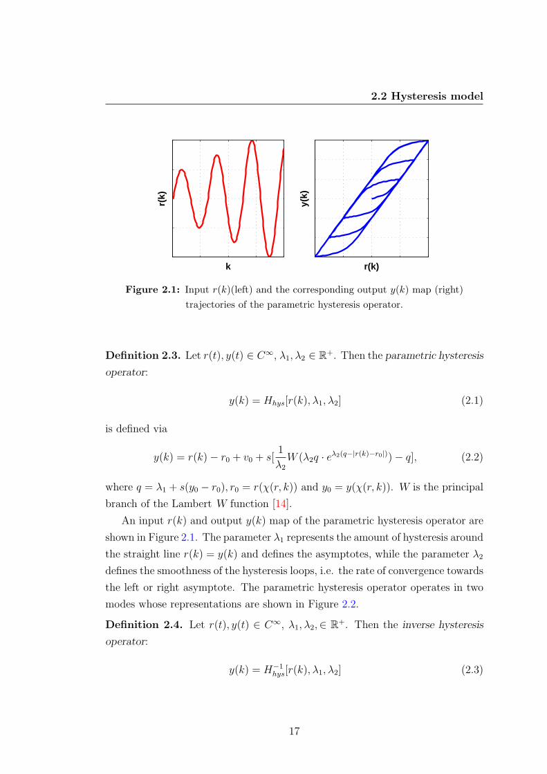
Figure 2.1: Input r(k)(left) and the corresponding output y(k) map (right)

trajectories of the parametric hysteresis operator.

Definition 2.3. Let r(t), y(t) ∈ C∞, λ1, λ2 ∈ R+. Then the parametric hysteresis

operator:

y(k) = Hhys[r(k), λ1, λ2] (2.1)

is defined via

y(k) = r(k)− r0 + v0 + s[1

λ2

W (λ2q · eλ2(q−|r(k)−r0|))− q], (2.2)

where q = λ1 + s(y0 − r0), r0 = r(χ(r, k)) and y0 = y(χ(r, k)). W is the principal

branch of the Lambert W function [14].

An input r(k) and output y(k) map of the parametric hysteresis operator are

shown in Figure 2.1. The parameter λ1 represents the amount of hysteresis around

the straight line r(k) = y(k) and defines the asymptotes, while the parameter λ2

defines the smoothness of the hysteresis loops, i.e. the rate of convergence towards

the left or right asymptote. The parametric hysteresis operator operates in two

modes whose representations are shown in Figure 2.2.

Definition 2.4. Let r(t), y(t) ∈ C∞, λ1, λ2,∈ R+. Then the inverse hysteresis

operator:

y(k) = H−1hys[r(k), λ1, λ2] (2.3)

17


2 0

0 0

( ( ) )2

2

( 1) ( 1)

1( )

ll

l

+ -

+ = + + - +

- ×m r k r

y k r k y r m

W m e

( 1)y k +

( 1)r k +

Yes

No

2 0

0 0

( ( ) )2

2

( 1) ( 1)

1( )

ll

l

- +

+ = + + - -

+ ×n r k r

y k r k y r n

W n e

[ ( 1) ( )][ ( ) ( 1)] 0+ - - - <r k r k r k r k

1 0 0l= - +m r y 1 0 0l= + -n r y

0 0=0, =0, 0*=r y k

( 1) ( ) 0+ - ³r k r k

Yes

No

0 0, ( ), ( )* * *= = =k k r r k y y k

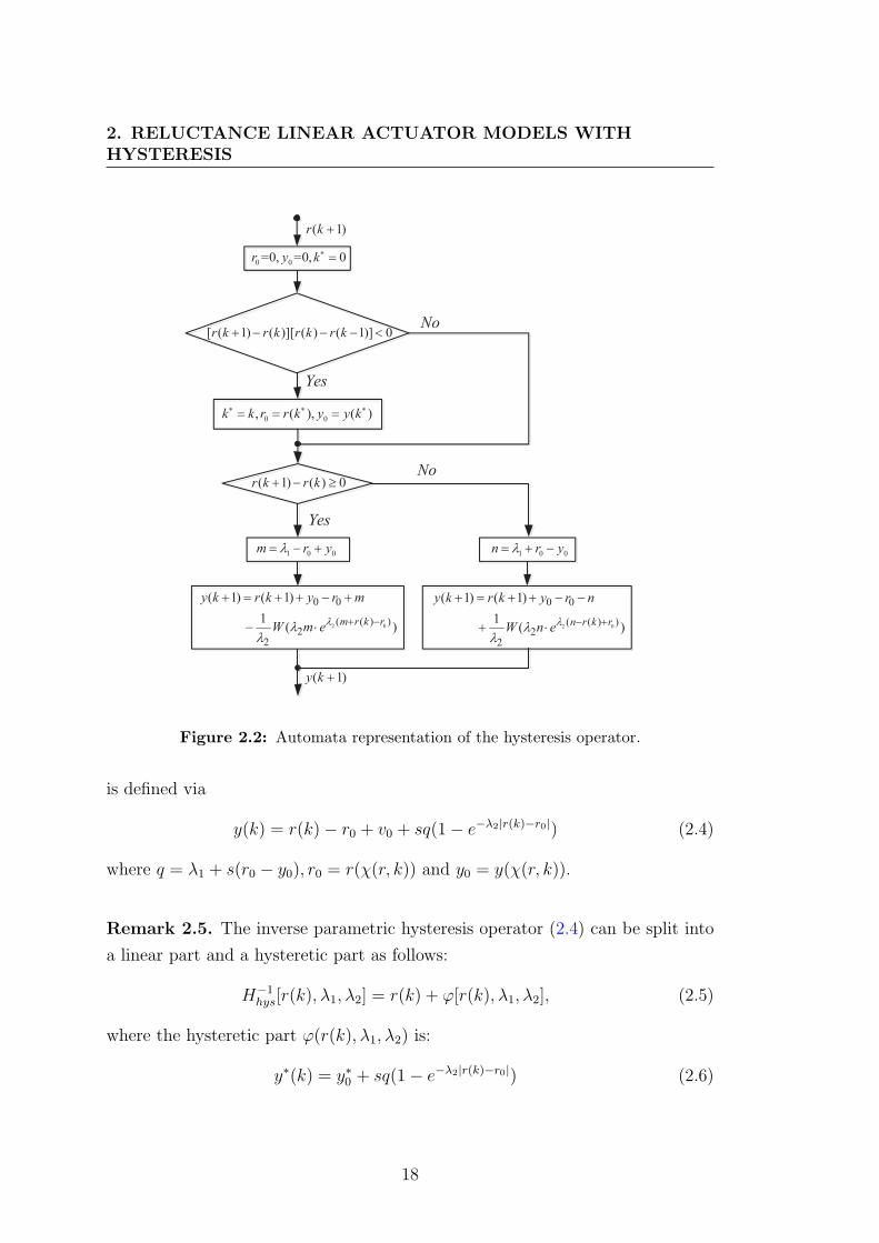
Figure 2.2: Automata representation of the hysteresis operator.

is defined via

y(k) = r(k)− r0 + v0 + sq(1− e−λ2|r(k)−r0|) (2.4)

where q = λ1 + s(r0 − y0), r0 = r(χ(r, k)) and y0 = y(χ(r, k)).

Remark 2.5. The inverse parametric hysteresis operator (2.4) can be split into

a linear part and a hysteretic part as follows:

H−1hys[r(k), λ1, λ2] = r(k) + φ[r(k), λ1, λ2], (2.5)

where the hysteretic part φ(r(k), λ1, λ2) is:

y∗(k) = y∗0 + sq(1− e−λ2|r(k)−r0|) (2.6)

18


H

B

Figure 2.3: H and B curve.

with q = λ1 − sv∗0, r0 = r(χ(r, k)) and v∗0 = v∗(χ(r, k)).

Propostion 2.6. For the hysteretic part φ of the inverse parametric hysteresis

operator defined in (2.6), ∀a, b > 0 the following holds:

limr→∞

{a · φ[b · r(k), λ1, λ2]− φ[r(k), a · λ1, b · λ2]} → 0 (2.7)

under the persistent excitation criterion that r(k) − r(k − 1), only at a finite

number of time instants k, i.e. the input u(k) is non-constant.

2.2.3 H and B model using hysteresis operator

However, the E-core coil uses the soft magnetic material, which has magnetic

hysteresis [6] between the magnetic field Hfe and the bulk magnetic flux density

Bfe. The typical Bfe−Hfe curve is illustrated in Figure 2.3. It is assumed that

the hysteretic Bfe−Hfe curve and the Hfe−Bfe curve of the core material can be

modeled [39] by the parametric hysteresis operator Equation (2.1) and the inverse

hysteresis operator Equation (2.3). Furthermore, since the input and output of

the hysteresis operators have to be in the same physical units, Bfe will be scaled

with 1µ0µr

. Then, we get the Bfe−Hfe curve model:

Bfe = Hhys(µ0µrHfe, λ1, λ2) (2.8)

and Hfe−Bfe curve model:

Hfe = H−1hys(

Bfe

µ0µr

, λ1, λ2). (2.9)

19


2.3 Models for reluctance linear actuator with

C-core

2.3.1 Magnetism principle

A brief introduction or review of magnetism will establish the basic ideas and

nomenclature exploited in the remainder of this discussion of electromagnets.

The total magnetic flux Φ passing through a surface A is the integral of flux

density B over the surface:

Φ =

∫∫A

B · dA. (2.10)

The magnetic field H and the magnetic induction (flux density) B are linked

by the constitutive law :

B = µ0µrH. (2.11)

Here, µ0 = 4π×10−7V s/Am stands for themagnetic permeability of a vacuum.

The relative permeability µr depends on the medium upon which the magnetic

field acts. For a vacuum, µr equals 1 and is also approximately unity in the air.

The SI unit of the magnetic field H is A/m.

2.3.2 Magnetic circuit

In the magnetic bearing technology, electromagnets or permanent magnets cause

the flux to circulate in a magnetic loop. When analyzing such magnetic loops, an

exact theoretical computation of the field is rarely possible and seldom required.

One usually works with analytic methods of approximation, based on the simpli-

fying assumption that the flux, except for in the air gap, runs entirely through

the iron (no leakage flux).

The field within the magnetic loop is assumed to be homogeneous both in the

iron and in the air gap. Therefore, we base our calculation on a mean length lfe

of the magnetic path and an air gap length of 2xg.

For the magnetic circuit in Figure 2.4∮H · dl = lfeHfe + 2xgHa = Ni (2.12)

20

2.3 Models for reluctance linear actuator with C-core

gx

i N

feA

B

/ 2F

/ 2F

aA

2+fe gl x

Figure 2.4: C-core I Magnetic circuit.

Follows from Amperes circuital law. From the flux density Bfe in the iron and Ba

in the air gap, field intensities Hfe and Ha from Equation (2.12) can be replaced

by Equation (2.11):

lfeµ0µr

·Bfe +2xg

µ0

·Ba = Ni. (2.13)

2.3.3 Flux density without hysteresis

Since the permeability µ = µ0µr of iron is considerably larger than that of air, the

magnetic field lines leave the iron almost perpendicularly to its surface. Both for

constant and alternating fields the computational methods used for static fields

are applied, which is admissible as long as the alternating fields have a very large

wavelength, compared with the geometry of the field.

For the computation of flux density B, the following simplifying assumptions

are made: Flux Φ runs entirely within the magnetic loop with iron cross section

Afe which is assumed to be constant along the entire loop and equal to cross-

21


section Aa in the air gap. From

Φ = BfeAfe = BaAa (2.14)

and

Afe = Aa, (2.15)

it follows that

Bfe = Ba. (2.16)

Solving Equation (2.13) for Ba yields

Ba = µ0Ni

(lfeµr

+ 2xg). (2.17)

In the iron, µr ≫ 1, so the magnetization of the iron is often neglected. In this

case, Equation (2.17) may be simplified to:

Ba = µ0Ni

2xg

. (2.18)

2.3.4 Energy in the air gaps

In this section, the simple reluctance actuator with a C-Core, as shown in Figure

2.4 is discussed.

The attraction force of magnets is generated at the boundaries between dif-

fering permeability µ. The calculation of these forces is based on the field energy.

We consider the energy Wa stored in the volume of the air gap, Va = 2xgAa.

In the case of the homogeneous field in the air gap of the magnetic loop, as

represented in Figure 2.4, the stored energy Wa obeys

Wa =1

2BaHaVa (2.19)

=1

2BaHaAa(2xg). (2.20)

In the following, we will discuss how to get the Ba(i, xg).

22

2.3 Models for reluctance linear actuator with C-core

2.3.5 Magnetic force without hysteresis

The force acting on the ferromagnetic body (µr ≫ 1) is generated by a change of

the field energy in the air gap, as a function of the body displacement. For small

displacements ds the magnetic flux BaAa remains constant.

When the air gap s increases by dxg, the volume increases by dVa = 2dxgAa,

and the energy Wa in the field increases by dWa. This energy has to be provided

mechanically, i.e. an attractive force has to be overcome. Thus, the force F

equals the partial derivative of the field energy Wa with respect to the air gap xg

(principle of virtual displacement):

F = −∂Wa

∂xg

(2.21)

= BaHaAa =B2

aAa

µ0

. (2.22)

In the case of a closed system, the force F can be derived from the principle

of virtual displacement. For electromagnets (Figure 2.4), electric energy is intro-

duced into the system through the coil terminals to set up the magnetic field. In

order for Equation (2.22) to remain valid, the differentiation has to be carried out

as if there is no electric energy exchange between the coil and its power supply,

i.e. when the flux density B remains constant. To derive force F as a function

of coil current and the air gap, Ba(i, xg) is inserted into Equation (2.22) after

differentiating.

To include the effect of iron with a constant, finite permeability µr, Equation

(2.18) will replace Ba in Equation (2.22). The force F resulting in this case, is

F = µ0

( Ni

lfe/µr + 2xg

)2

Aa. (2.23)

Neglecting the Iron

In the simplest case where the iron is neglected, Ba is replaced by Equation (2.17).

From Equation (2.22), the resulting force F is

F = µ0Aa(Ni

2xg

)2 =1

4µ0N

2Aai2

x2g

= ηi2

x2g

(2.24)

in which η = 14µ0N

2Aa, and the area Aa is assumed to be the projected area of

the pole face, rather than the curved surface area.

23


2.3.6 Flux density with hysteresis

From Ha = Ba

µ0and by substituting Equation (2.9), Equation (2.13) is rewritten

as:

i =2xg

µ0N·Ba +

lfeN

·H−1hys(

Bfe

µ0µr

, λ1, λ2). (2.25)

From Equation (2.16), Equation (2.25) can be rewritten as:

i =2xg

µ0N·Ba +

lfeN

·H−1hys(

Ba

µ0µr

, λ1, λ2). (2.26)

Splitting the hysteresis operator in Equation (2.26) as in Equation (2.5) yields:

i =Ba

µ0N(2xg +

lfeµr

) +lfeN

· φ( Ba

µ0µr

, λ1, λ2). (2.27)

After appling Proposition 2.6, Equation (2.27) becomes:

i =Ba

µ0N(2xg +

lfeµr

) + φ( Ba

µ0N(2xg +

lfeµr

), λ∗1, λ

∗2

)= H−1

hys

( Ba

µ0N(2xg +

lfeµr

), λ∗1, λ

∗2

). (2.28)

where λ∗1 =

lfeNλ1 and λ∗

2 =1

(2xgµrAfe

Aa+lfe)

λ2. Then from Equation (2.28), we get:

Ba =µ0N

2xg +lfeµr

·Hhys(i, λ∗1, λ

∗2). (2.29)

In the iron, µr ≫ 1, so the magnetization of the iron is often neglected, then

Equation (2.29) may be simplified as:

Ba =µ0N

2xg


∗2). (2.30)

2.3.7 Magnetic force with hysteresis

Then by substituting Equation (2.30) into Equation (2.22), a new reluctance

actuator model with hysteresis is obtained as:

F =µ0AaN

2

4· (Hhys(i, λ

∗1, λ

∗2))

2

x2g

. (2.31)

24

2.4 Models for reluctance linear actuator with E-core

i

a

b

a

a

a

w

a a

w

1l

1l

2l

1l

1l

gx

Figure 2.5: E-core structure.

Neglecting the Iron

By substituting Equation (2.29) into Equation (2.22), a new reluctance actuator

model with hysteresis is obtained as:

F = µ0AaN2 · (Hhys(i, λ

∗1, λ

∗2))

2

(2xg +lfeAa

µrAfe)2

. (2.32)

2.4 Models for reluctance linear actuator with

E-core

In this section, the models for reluctance linear actuator with E-core as shown in

figure 2.5 is discussed.

2.4.1 Magnetic circuit

For the magnetic circuit in Figure 2.5, it follows from Amperes circuital law that

Ni = Hfe1 · l2 +Hfe5 · l1 +Hfe7 · l1 +Ha1 · xg

25


1F

1F

1F

1F

1F

1F

1F

2F

1F

1aA1feA

2aA2feA

3aA3feA4feA

6feA

5feA

7feA

Figure 2.6: E-core flux circuit

+ Hfe2 · l2 +Ha2 · xg

+ Hfe4 · l1 +Hfe3 · l2 +Hfe6 · l1 +Ha3 · xg

+ Hfe2 · l2 +Ha2 · xg (2.33)

From the flux density Bfe in the iron and Ba in the air gap, field intensities

Hfe and Ha from Equation (2.33) can be replaced by Equation (2.11):

Ni =Bfe1

µ0µr

· l2 +Bfe5

µ0µr

· l1 +Bfe7

µ0µr

· l1 +Ba1

µ0

· xg

+Bfe2

µ0µr

· l2 +Ba2

µ0

· xg

+Bfe4

µ0µr

· l1 +Bfe3

µ0µr

· l2 +Bfe6

µ0µr

· l1 +Ba3

µ0

· xg

+Bfe2

µ0µr

· l2 +Ba2

µ0

· xg. (2.34)

26


2.4.2 Flux density without hysteresis

For the computation of flux density B, from Figure 2.5, a flux circuit as shown in

Figure 2.6, the following simplifying assumptions are made: Flux Φ runs entirely

within the magnetic loop with iron cross section Afe1, Afe3, Afe4, Afe5,Afe6, Afe7,

which are assumed to be constant along the entire loop and equal to cross-section

Aa1 and Aa3 in the air gap, we get:

Φ1 = Bfe1Afe1

= Bfe3Afe3

= Bfe4Afe4

= Bfe5Afe5

= Bfe6Afe6

= Bfe7Afe7

= Ba1Aa1

= Ba3Aa3 (2.35)

Aa = Afe1

= Afe3

= Afe4

= Afe5

= Afe6

= Afe7

= Aa1

= Aa3, (2.36)

Let Bfe be the flux density in the iron, then

Bfe = Bfe1

= Bfe3

= Bfe4

= Bfe5

27


1F

1F

1F

2F

1F

1aA1feA

2aA2feA

3aA3feA

Figure 2.7: Simplified flux circuit

= Bfe6

= Bfe7. (2.37)

Further, Ba be the flux density in the air gap and

Ba = Ba1

= Ba3. (2.38)

Then from Equations (2.35), (2.36), (2.37) and (2.38), we get

Bfe = Ba. (2.39)

From Equations (2.35), (2.36), (2.37), (2.38) and (2.39) and Figure 2.6, a simpli-

fied flux circuit is shown in Figure 2.7, in which

Φ1 = BfeAa

= BaAa. (2.40)

28


Then from Figure 2.6, we get:

Φ2 = 2Φ1

= 2BfeAa

= 2BaAa. (2.41)

When b = a as shown in Figure 2.5:

Afe2 = Aa2 = Aa (2.42)

Then from Equation (2.41) and (2.42), we get:

Bfe2 = Ba2 (2.43)

Bfe2 = 2Bfe (2.44)

Ba2 = 2Ba (2.45)

From Equations (2.37), (2.38), (2.44) and(2.45), Equation (2.34) can be rewrit-

ten as:

Ni =Bfe

µ0µr

· l2 +Bfe

µ0µr

· l1 +Bfe

µ0µr

· l1 +Ba

µ0

· xg

+2Bfe

µ0µr

· l2 +2Ba

µ0

· xg

+Bfe

µ0µr

· l1 +Bfe

µ0µr

· l2 +Bfe

µ0µr

· l1 +Ba

µ0

· xg

+2Bfe

µ0µr

· l2 +2Ba

µ0

· xg. (2.46)

Define lm1 = 4l1 + 6l2. Equation (2.46) can be rewritten as:

Ni =Bfe

µ0µr

· lm1 +Ba

µ0

· 6xg. (2.47)

Then, from Equation (2.47) and (2.39), Ba becomes:

Ba =Niµ0

lm1

µr+ 6xg

. (2.48)


case, Equation (2.48) may be simplified:

Ba =Niµ0

6xg

(2.49)

29


When b = 2a as shown in Figure 2.5:

Afe2 = Aa2 = 2Aa (2.50)

Then from Equation (2.41) and (2.50), we get:

Bfe2 = Ba2 (2.51)

Bfe2 = Bfe (2.52)

Ba2 = Ba. (2.53)

From Equations (2.37), (2.38), (2.52) and(2.53), Equation (2.34) can be rewrit-

ten as:

Ni =Bfe

µ0µr

· l2 +Bfe

µ0µr

· l1 +Bfe

µ0µr

· l1 +Ba

µ0

· xg

+Bfe

µ0µr

· l2 +Ba

µ0

· xg

+Bfe

µ0µr

· l1 +Bfe

µ0µr

· l2 +Bfe

µ0µr

· l1 +Ba

µ0

· xg

+Bfe

µ0µr

· l2 +Ba

µ0

· xg. (2.54)

Define lm2 = 4l1 + 4l2. Equation (2.54) can be rewritten as:

Ni =Bfe

µ0µr

· lm2 +Ba

µ0

· 4xg, (2.55)

From Equation (2.55) and (2.39), Ba turns to:

Ba =Niµ0

lm2

µr+ 4xg

. (2.56)


case, Equation 2.56 may be simplified as:

Ba =Niµ0

4xg

. (2.57)

30


2.4.3 Energy in the air gaps

In the case of homogeneous field in the air gap of the magnetic loop, as represented

in Figure 2.5, the stored energy Wa obeys:

Wa =1

2Ba1Ha1Va1 +

1

2Ba2Ha2Va2 +

1

2Ba3Ha3Va3

=1

2

(Ba1Ha1Aa1 +

1

2Ba2Ha2Aa2 +

1

2Ba3Ha3Aa3

)xg

=1

2

(B2a1

µ0

Aa1 +B2

a2

µ0

Aa2 +B2

a3

µ0

Aa3

)xg (2.58)


From (2.36), (2.38), (2.42), (2.45), Equation (2.58) can be rewritten as

Wa =1

2

[B2a

µ0

Aa +(2Ba)

2

µ0

Aa +B2

a

µ0

Aa

]xg

=3B2

aAaxg

µ0

. (2.59)


From (2.36), (2.38), (2.50), (2.53), Equation (2.58) can be rewritten as

Wa =1

2

[B2a

µ0

Aa +B2

a

µ0

2Aa +B2

a

µ0

Aa

]xg

=2B2

aAaxg

µ0

. (2.60)

2.4.4 Magnetic force without hysteresis


From Equation (2.59), force F equals the partial derivative of the field energy Wa

with respect to the air gap xg (principle of virtual displacement):

F = −∂Wa

∂xg

=3B2

aAa

µ0

. (2.61)

From Equation (2.48) and (2.61), we get:

F = 3N2µ0Aai2

( lm1

µr+ 6xg)2

. (2.62)

31


Neglecting the Iron


F =1

12N2µ0Aa

i2

x2g

. (2.63)


From Equation (2.60), force F equals the partial derivative of the field energy Wa

with respect to the air gap xg (principle of virtual displacement):

F = −∂Wa

∂xg

=2B2

aAa

µ0

(2.64)


F = 2N2µ0Aai2

( lm2

µr+ 4xg)2

. (2.65)

Neglecting the Iron


F =1

8N2µ0Aa

i2

x2g

. (2.66)

2.4.5 Flux density with hysteresis


By substituting Equation (2.9), Equation (2.47) becomes:

i =Ba

µ0N· 6xg +

lm1

N·H−1

hys

( Bfe

µ0µr

, λ1, λ2

). (2.67)

Splitting the hysteresis operator in Equation (2.67) as in Equation (2.5) yields

i =Ba

µ0N(6xg +

lm1

µr

) +lm1

N· φ( Ba

µ0µr

, λ1, λ2). (2.68)

After applying Proposition 1.6, Equation (2.68) becomes

i =Ba

µ0N(6xg +

lm1

µr

) + φ(Ba

µ0N(4xg +

lm1

µr

), λ∗1, λ

∗2)

= H−1hys

( Ba

µ0N(4xg +

lm1

µr

), λ∗1, λ

∗2

)(2.69)

32


where λ∗1 =

lm1

Nλ1 and λ∗

2 =1

(4xgµr+lm1)λ2. From Equation (2.69), we get:

Ba =µ0N

(6xg +lm1

µr)·Hhys(i, λ

∗1, λ

∗2). (2.70)


case, Equation 2.70 may be simplified to:

Ba =µ0N

6xg


∗2). (2.71)


By substituting Equation (2.9), Equation (2.55) can be rewritten as:

i =4xg

µ0N·Ba +

lm2

N·H−1

hys(Ba

µ0µr

, λ1, λ2). (2.72)

Splitting the hysteresis operator in Equation (2.72) as in Equation (2.5) yields

i =Ba

µ0N(4xg +

lm2

µr

) +lm2

N· φ( Ba

µ0µr

, λ1, λ2). (2.73)

After applying Proposition 1.6, Equation (2.73) becomes

i =Ba

µ0N(4xg +

lm2

µr

) + φ( Ba

µ0N(4xg +

lm2

µr

), λ∗1, λ

∗2

)= H−1

hys

( Ba

µ0N(4xg +

lm2

µr

), λ∗1, λ

∗2

)(2.74)

where λ∗1 =

lm2

Nλ1 and λ∗

2 =1

(4xgµr+lm2)λ2. From Equation (2.74), we get:

Ba =µ0N

(4xg +lm2

µr)·Hhys(i, λ

∗1, λ

∗2). (2.75)


case, Equation (2.70) may be simplified to:

Ba =µ0N

4xg


∗2). (2.76)

33


2.4.6 Magnetic force with hysteresis



F = 3N2µ0Aa(Hhys(i, λ

∗1, λ

∗2))

2

( lm1

µr+ 6xg)2

. (2.77)

Neglecting the Iron


F =1

12N2µ0Aa

(Hhys(i, λ∗1, λ

∗2))

2

x2g

. (2.78)



F = 2N2µ0Aa(Hhys(i, λ

∗1, λ

∗2))

2

( lm2

µr+ 4xg)2

. (2.79)

Neglecting the Iron


F =1

8N2µ0Aa

(Hhys(i, λ∗1, λ

∗2))

2

x2g

= η(Hhys(i, λ

∗1, λ

∗2))

2

x2g

(2.80)

This model contains both the hysteresis and obvious square linearity between

the input and output. If the reluctance actuator is modeled by Equation (2.80),

the curves of input current and the corresponding output force are obtained as

shown in Figure 2.8. It can be seen that the hysteresis model Equation (2.80)

provides a good approximation for the hysteresis phenomenon between the input

current i and output force F .

2.5 Conclusion

The reluctance linear actuator models are discussed in this chapter. The para-

metric hysteresis operator is reviewed firstly. Further, the models without hys-

teresis for reluctance linear actuator with C-core and E-core are reviewed; the

34

2.5 Conclusion

0 30 600

1

2

t

curr

ent

0 1 20

100

180

current

Fo

rce

Figure 2.8: Curve of an input current and the corresponding output force based

on the current-driven reluctance actuator model with hysteresis

models with hysteresis for reluctance linear actuator with C-core and E-core are

proposed.

35


36

3

Nonlinear Control for Reluctance

Linear Actuator

3.1 Introduction

In this chapter, the basic control method and nonlinear current control for reluc-

tance actuator are reviewed.

3.2 Control of reluctance linear actuator

3.2.1 Nonlinear current compensation

A typical structure of the current-driven reluctance linear actuator control is

shown in Figure 3.1. Due to the unstable nature of the electromagnetic forces,

Set

PointdF idiNonlill nii ear

CoCC mpensator

Nonlinear

Compensator

Power

Amplill fii iff er

Power

Amplifier

Reluctance

Actuator

Reluctance

ActuatorCC MassMassF

Position

Sensor

Position

Sensor

gx

Figure 3.1: Typical current-driven reluctance actuator control loop.

37

3. NONLINEAR CONTROL FOR RELUCTANCE LINEARACTUATOR

a feedback control loop is required to achieve stable performance. In Figure

3.1, “C”denotes a linear position controller such as the proportional-integral-

derivative (PID) controller, which guarantees the stability of the closed loop. The

position controller uses the position in the air gap measured by a position sensor

to generate the force command Fd. The power amplifier supplies the current for

the reluctance actuator.

From Equation (2.24), a nonlinear current compensator can be obtained [80]

as

id =

√Fd · x2

g

ηd(3.1)

where ηd is the estimate of real constant η.

The above nonlinear current compensator does not consider the hysteresis in

the reluctance force. From the analysis of the hysteresis influence in the introduc-

tion, it is necessary to find a hysteresis compensation method for the reluctance

linear actuator in the high-precision positioning.

3.2.2 Control of a stage having paired reluctance linear

actuator

Usually, six motion directions of the fine stage in a lithographic tool are defined

in a coordinate system [8] and six separate single-input single output controller

can be decoupled for each motion direction. In this section, only one motion

direction is considered, such as the scanning direction. The fine stage is supported

vertically by anti-friction bearings such as air bearings. The size of the wafer

stage is corresponding to the circular wafer having a diameter of 200, 300, or

450 mm. Due to the nature of reluctance force, an E/I core actuator can only

generate a unidirectional attractive force. To generate an active force in the

opposite direction, a second actuator needs to be placed on the opposite side.

Figure 3.2 illustrates a simplified one motion direction fine stage [80] having

paired reluctance actuators E-core 1 and E-core 2. The material of fine stage is

the carbon fiber to reduce the weight for the higher acceleration. The material

of the E-core and the I-target is the Cobalt-Iron.

38

3.2 Control of reluctance linear actuator

stage

E-core 2 E-core 1

1gx2gx

1i2i1F2F

x

Fine

stage

Figure 3.2: Paired E/I core actuator.

The gaps between the E-core 1,2 and the stage are xg1 and xg2, which can

be measured by suitable sensors such as capacitor sensor. The force F1 and F2

are nonnegative, while the difference between F1 and F2 can take any value and

direction. In the initial state, the gaps are xg1 = xg0 and xg2 = xg0, where xg0

is the initial gap. In Figure 3.2, we define the right as the positive direction.

Furthermore, when the stage moves to the positive direction, the gaps become

xg1 = xg0 − x and xg2 = xg0 + x respectively where x is the global placement and

can be measured by position sensor such as a laser interferometer [80].

A conventional control scheme is depicted in Figure 3.3, in which the controller

C(s) is formed by a proportional-integral-derivative (PID) controller, a lowpass

filte and a lead compensatorr. In the feedback loop, the controller uses the

position of the stage measured by a position sensor to generate the applied force

command. The filter Q(s) generates a feedforward force based on the setpoint

position. When P (s) is described by 1/ms2, Q(s) = ms2 generats a force that is

proportional to the setpoint acceleration.

The final position accuracy is determined by measurement system errors, dis-

turbance forces including the nonlinearity force caused by the hysteresis, which

have an effect on the closed loop performance. Rejection of output (measure-

ment) disturbances and input (force) disturbances is judged by, respectively, the

39


( )P s( )C s

( )Q s

+

+

setpoint

position

+-

Figure 3.3: Basic control scheme.

output sensitivity

Gos =1

1 + P (s)C(s)(3.2)

and the process sensitivity

Gps =P (s)

1 + P (s)C(s). (3.3)

Based on the conventional controller shown in Figure 3.3, a control loop for

the fine stage having paired E/I core actuator is shown in Figure 3.4. Gs(s)

denotes the position controller, Qs(s) denotes the feedforward controller, Ps(s)

denotes the fine stage process, “EI1”and “EI2”denote the E-core 1 and E-core2,

“NC1”and “NC2”denote nonlinear current compensator and “FD”denotes the

force distribution.

In Figure 3.4, “FD”distributes the desired force to each E/I core actuator as

follows:

Fd1=F0 + Fd/2, (3.4)

Fd2=F0 − Fd/2 (3.5)

where F0 is the bias force generated by paired E/I core actuator respectively in the

opposite direction, which provides a zero net force on the stage, thus maintaining

the position of the stage. In this chapter, F0 is determined as F0 = Fmax/2,

in which Fmax is the maximum force corresponding the maximum acceleration.

More details about how to select the bias force F0 can be found in patent [12].

40

3.3 Conclusion

( )sC s

+

+

setpoint

position

+-

seFD

NC1

NC2

( )sP s

EI1

EI2

+

-

sx

2gx

Acceleration

feedforward

x

dF F1dF

2dF

1i

2i

1F

2F

1gx

( )Q s

Figure 3.4: Paired E/I core actuator control.

Since there exits strong linearity between the input current i and output force

F , from Equation (3.1), nonlinear current compensators “NC1”and “NC2”can be

obtained as

i1 =

√Fd1 · x2

g1

ηd, (3.6)

i2 =

√Fd2 · x2

g2

ηd, (3.7)

where ηd is the estimate of real constant η. However, the reluctance actuator

use the soft magnet material, which has a hysteresis between the input current

i and output force F in reluctance actuators “EI1”and “EI2”as shown in Figure

3.4. Since the nonlinear current compensators “NC1”and “NC2”can not com-

pensate the hysteresis between the input current i and output force F in each

E/I actuator, a hysteresis force results in between the position controller force

command Fd and the real output force F . However, the hysteresis influence must

be considered in the high-precision positioning [39], so it is necessary to find a

hysteresis compensation method for the reluctance linear actuator.

3.3 Conclusion

In this chapter, the basic control method and nonlinear current control for reluc-

tance actuator are reviewed.

41


42

4

Hysteresis Compensation for a

Current-driven Reluctance Linear

Actuator Using Adaptive MNN

4.1 Introduction

A variety of models and compensation algorithms have been developed for the

hysteresis [36][32][1][87]. The classical approach is to construct a hysteresis in-

verse and use it as a feed-forward compensator [32] together with a feedback

control. The hysteresis compensation method via Preisach model inversion has

been proposed in [55]. An inverse parametric hysteresis model [39] was used in

current-mode operated reluctance force actuator. However, the above methods

need precise hysteresis model, which is usually complex and hard to obtain.

Owing to the online self-learning and estimation capability of the neural net-

work, it provides a good solution for solving nonlinear problems. Especially, the

multi-layer neural network (MNN) is effectively used in nonlinear discrete-time

system identification and control [49]. Although a lot of researches have been

done on the neural network application to the hysteresis [61] [20], the neural net-

work compensation for the current-driven reluctance actuator with hysteresis has

yet to be studied.

The main contributions of this section is a hysteresis compensator for current-

driven reluctance linear actuator using the adaptive MNN proposed for the first

43

4. HYSTERESIS COMPENSATION FOR A CURRENT-DRIVENRELUCTANCE LINEAR ACTUATOR USING ADAPTIVE MNN

time. Concretely speaking, based on the input-output feature of the hysteresis in

reluctance force and the learning and approximation ability of neural network, a

hysteresis current compensator is proposed for the current-driven reluctance ac-

tuator with hysteresis using the adaptive MNN [49], whose weight is updated by

the error between the desired force and the actual force. The main advantage of

the proposed compensation method is that the inverse hysteresis model does not

be required. Simulations are conducted on the reluctance actuator model with

hysteresis and the results show that the adaptive MNN is effective in overcom-

ing the hysteresis and promising in high precision and high acceleration control

applications.

4.2 Neural network

Since McCulloch and Pitts [62] introduced the idea of studying the computa-

tional abilities of networks composed of simple models of neurons in the 1940s,

neural network techniques have been successfully applied in many fields such

as learning, pattern recognition, signal processing, modelling and system con-

trol. The approximation abilities of neural networks have been proven in many

research works [15][22][13][71][31]. The early works on neural network applica-

tions to controller design were reasearched in [86][2][69][35][64]. In the late 1980s,

the popularization of backpropagation (BP) algorithm [70] greatly boosted the

development of neural control and many neural control approaches have been

developed [60][59]. The analytical results obtained in [21][46] showed that using

multi-layer neural networks as function approximators could guarantee the sta-

bility of the systems when the initial network weights chosen were sufficiently

close to the ideal weights.

Recently, neural networks have been made particularly attractive and promis-

ing for applications to modelling and control of nonlinear systems. For neural

network controller design of general nonlinear systems, several researchers have

suggested to use neural networks as emulators of inverse systems. Using the im-

plicit function theory, the NN control methods proposed in [28] [46] have been

used to emulate the ”inverse controller” to achieve the desired control objectives.

Based on this idea, an adaptive controller has been developed using high order

44

4.2 Neural network

neural networks with stable internal dynamics in [90] and applied in [25]. As an

alternative, neural networks have been used to approximate the implicit desired

feedback controller in [24].

In nonlinear system control, neural networks can be applied as a function

approximators to emulate the ”inverse” control. For example, neural networks

combined backstepping design are reported in [27][85], using neural networks to

construct observers can be found in [57][16], neural network control in robot

manipulators are reported in [76][81][82], neural control for distillation column

are reported in [72].

HONN(high order neural networks), RBF(Radial basis function neural net-

works) and MNN(multi-layer neural network) are three kinds of frequently used

neural networks in nonlinear system control and identification[85][3]. HONN and

RBF networks can be considered as two-layer networks, in which the input space

is mapped on to a new space. The output layer combines the outputs in the latter

space linearly. MNN is a static feed-forward network that consists of a number

of layers, each layer having a number of McCulloch-Pitts neurons [62]. Due to its

hidden layers, the MNN has an important character that it can approximate any

continuous nonlinear function. Once the hidden layers have been selected, only

the adjustable weights have to be determined to specify the networks completely.

Since each node of any layer is connected to all the nodes of the following layer, it

follows that a change in a single parameter at any one layer will generally affect

all the outputs in the following layers. MNNs with one or more hidden layers are

capable of approximating any continuous nonlinear function, which was shown

independently by [22][13][71]. This important character makes it one of the most

widely used neural networks in system modelling and control.

In this thesis, the MNN will be used to compensate the hysteresis in the

reluctance linear actuator.

45


MassMassdF i

F

di

ci

Adaptive laws

e

WV

Hysteresis Current Compensator

Nonlill nii ear

CoCC mpensator

Nonlinear

Compensator

ddi ower

Amplill fi iff er

Power

Amplifier

Reluctance

Actuator

Reluctance

Actuator

MNN

AccelerometerAccelerometerma

Figure 4.1: Structure of hysteresis current compensator using adaptive MNN.

4.3 Design of nonlinear current compensator us-

ing adaptive MNN

A typical structure of the current-driven reluctance linear actuator control is

shown in Figure 3.1. Due to the unstable nature of the electromagnetic forces, a

feedback control loop is required to achieve stable performance.

The nonlinear current compensator (3.1) does not consider the hysteresis in

the reluctance force. From the analysis of the hysteresis influence in introduc-

tion, it is necessary to find a hysteresis compensation method for the reluctance

linear actuator in the high-precision positioning. In the following, a hysteresis

compensator for the reluctance linear actuator based on the adaptive MNN will

46

4.3 Design of nonlinear current compensator using adaptive MNN

be apposed.

Owing to the advantages of MNN, a hysteresis current compensator using the

adaptive MNN can be obtained as shown in Figure 4.1 for the current-driven

reluctance actuator force. The feedback force F can be estimated from the rela-

tion F = ma, with m being the stage mass and a the actual acceleration. The

actual acceleration a can be measured by an accelerometer or computed from the

measured gap position xg by a digital double differentiator. The double differ-

entiation may introduce a noise. However, when a filter such as the least-square

method and considering the noise level makes double differentiation acceptable as

a method to calculate the stage acceleration [9]. In this section, the acceleration

a is assumed to be measured by the accelerometer. The detail of the adaptive

MNN is as follows.

The current command id(k) is compensated by the output ic(k) of the adaptive

MNN

idd(k) = id(k) + ic(k). (4.1)

At instant k, the nonlinear term ic(k) in Equation (4.1) is estimated by the

following MNN

ic(k) = WT(k)S(VT(k)x(k)). (4.2)

Here, W(k) ∈ Rl+1 and V(k) ∈ R(2n+1)×l are weighting matrices, l is the num-

ber of hidden-layer neurons, x(k) = [xT (k), 1]T denotes the input vector of the

neural network, xT (k) = [Fd(k+ 1), Fd(k), F (k+ 1), F (k)], and S(VT(k)x(k)) =

[s(vT1 (k)x(k)), · · · , s(vT

l (k)x(k)),1]T with s(x) = 1/(1 + e−x).

The MNN estimation error is

ε(k + 1) = Fd(k)− F (k). (4.3)

The adaptive update law of the neural network weight is chosen as

W(k + 1) = W(k)− ProjW [γwS(k)ε(k + 1)] (4.4)

V(k + 1) = V(k)− ProjV[γvzlWT (k)S′(t)ε(k + 1)] (4.5)

47


where γw and γv are the learning rates with positive constants, S(k) = diag{s1(k), · · · , sl(k)}with si(k) = s(vTi x(k)), zl = [1/

√l, · · · , 1/

√l]T (∥z∥ = 1) is a vector compati-

ble with V(k). S′(k) = diag{s′1(k), · · · , s′l(k)} is a diagonal matrix with s′i(k) =

s′(vTi x(k)). Since the output of the hidden layer neural network is directly related

to the input of the output weight, the output weight is introduced in Equation

4.5. The projection function Projθ(∗) is defined as Projθ(∗) = {Projθ(∗jk)} whose

element in the j-th row and k-th column is:

Projθ(∗jk) =

−∗jk(

θjk = ρθjk,max and ∗jk < 0θjk = ρθjk,min and ∗jk > 0,

)jk otherwise

(4.6)

where ∗ is either a vector or matrix with its element being ∗jk, ρθjk,min and ρθjk,max

are presumed upper and lower bound of θij, and θ denotes W and V. However,

due to the fact that those bounds may not be known a priori, certain fictitious

large enough bounds can be used [29]. We just need to limit the output amplitude

of the output of adaptive MNN (4.1), e.g. limit the power amplifier input within

±10 v.

4.4 Simulations

Example 1: A simulation for the current-driven reluctance actuator is conducted

to verify the performance of the proposed hysteresis compensation configuration

shown in Figure 4.1.

Items Values

the maximum force 200 N

the maximum gap xg 0.4 mm

the E/I constant k = 7.73× 10−6

Table 4.1: E/I core parameters.

In this simulation, since the linear power amplifier has a high bandwidth and

rapid response, it is ignored. When a force command Fd is imposed without a

counter balance force, the I-target would be pulled to the E-core. For this reason,

it is assumed that the I-target is fixed, so that we may investigate the force

48

4.4 Simulations

0 2 4 6 8 10 12 14 160

50

100

150

200

t [s]

Ref

eren

ce F

orc

e [N

]

Figure 4.2: Reference force.

0 50 100 150 200−2

−1.5

−1

−0.5

0

0.5

1

1.5

2

Reference force

Fo

rce

erro

r [N

]

Without Hysteresis CompensationWith Hysteresis Compensation

Figure 4.3: Comparison of the force error between force generations without

hysteresis compensation and with hysteresis compensation.

49


tracking performance. The reluctance linear actuator with hysteresis is modeled

by Equation (2.80), whose parameters chosen as in the patent [12] as shown in

table (4.1):

To reproduce a reluctance actuator model with non-smooth hysteresis, the

parameter λ2 of the hysteretic operator Equation (2.80) would have to be infinitely

large. Here, the hysteresis operator parameters are chosen as λ1 = 0.02 and

λ2 = 10.

The control objective is to make the system output F following the reference

force Fd. A non-trivial reference force depicted in Figure 4.2. This profile is

used to test the proposed nonlinear controller with hysteresis compensation with

respect to higher order reversal curves. The adaptive MNN compensator (4.1)

is designed to compensate the hysteresis. The parameters of the adaptive MNN

are determined as: the input vector of the neural network is chosen as x(k) =

[Fd(k + 1), Fd(k), F (k + 1), F (k)], the number of hidden-layer neurons is l = 40,

the initial neural network weighting matrices are w(0) = 0 and v(0) = 0, the

learning rate are selected as γw = 0.0006 and γv = 0.01 respectively.

The maps between the reference force Fd(k) and the output force F (k) track-

ing error with nonlinear current control without hysteresis compensation and with

hysteresis compensation are shown in Figure 4.3. The largest force tracking error

without hysteresis compensation is about ±2 N . With hysteresis compensation,

it is about ±0.1 N . Furthermore, Figure 4.4 shows that the ratio between the

output force F (k) and its reference command Fd(k) with and without hysteresis

compensator, and the ratio with hysteresis compensation is very close to 1 with

compensation. From the simulation results, it is clear that the force with hystere-

sis compensation has a much smaller force tracking error than without hysteresis

compensation.

Example 2: In order to verify if the proposed hysteresis compensation method

can be applied in high-precision systems, we do the following simulation using

the reluctance actuator to drive a one degree of freedom stage.

Due to the nature of the reluctance force, an E/I core actuator can only

generate a unidirectional attractive force. To generate an active force in the

opposite direction, a second actuator needs to be placed on the opposite side of

the I-Target as shown in Figure 3.2, in which including electromagnetic actuators

50

4.4 Simulations

0 20 40 60 80 100 120 140 160 180 2000

20

40

60

80

100

120

140

160

180

200

Reference Force

Ou

tpu

t F

orc

e


80 100 12050

100

150

Figure 4.4: Comparison of the force hysteresis loop between force generations

without hysteresis compensation and with hysteresis compensation.

E-core 1 and E-core 2 as well as a stage [12]. Choose Equation (2.80) as the

E/I core actuator model with hysteresis. The gap xg1 separates the E-core 1

and the I-target 1 and the gap xg2 separates E-core 2 and I-target 2. The stage

parameters are shown in table (4.2)

Items Values

the stage mass 10 kg

the position sensor resolution 1 nm

the sampling time 0.5ms

the bias force F0 = 15 N

The E-core electromagnetic constant k = 7.73× 10−6

Table 4.2: E/I stage simulation parameters.

The gap xg1 and xg2 between the E-core 1,2 and the I-target1,2 are in the

range of 0 µm to 400 µm and the initial gap is xg0 = 400 µm. The parameters

of hysteresis operator are set as in Example 1.

The stage control system uses the proportional-integral (PI) controller to guar-

51


0 0.01 0.02 0.03 0.04 0.05 0.06 0.07 0.080

0.2

0.4P

ositi

on [m

m]

0 0.01 0.02 0.03 0.04 0.05 0.06 0.07 0.080

5

10

t (sec)

Vel

ocity

[mm

/s]

Figure 4.5: Reference position and velocity.

antee the stability of the closed-loop position system, while the adaptive MNN

hysteresis compensator is employed to reduce the influence of the hysteresis and

improve the performance of the closed-loop position system. The adaptive MNN

parameters for the two E/I actuators are the same as Example 1.

The control objective is to make the stage position x follow the reference

position. The reference trajectory is determined by the 3rd order trajectory

planning method [43]. The position and velocity are shown in Figure 4.5. The

trajectory values are shown in table (4.3).

Items Values

the largest displacement 350 µm

the maximum velocity 10 mm/s

the maximum acceleration 1 m/s2

the jerk 200 m/s3

Table 4.3: Trajectory values.

The position tracking errors of control without hysteresis compensation and

with hysteresis compensation are shown in Figure 4.6. We define the constant

velocity settling time and the stop time as the time instants after which the po-

sition tracking error is less than 1 µm. From the enlarged view of the constant

velocity segment shown in Figure 4.7, it can be seen that the constant veloc-

52

4.4 Simulations

0 0.01 0.02 0.03 0.04 0.05 0.06 0.07 0.08−30

−20

−10

0

10

20

30

t (sec)

Tra

ckin

g E

rro

r [u

m]


ConstantVelocity Stop

Figure 4.6: Comparison of the position tracking error between controls without

hysteresis compensation and with hysteresis compensation.

0.015 0.02 0.025 0.03 0.035−4

−3

−2

−1

0

1

2

3

4

t (sec)

Tra

ckin

g E

rro

r [u

m]


0.015s 0.0198s


hysteresis compensation and with hysteresis compensation in the constant

velocity segment.

53


0.05 0.055 0.06 0.065 0.07 0.075 0.08−4

−3

−2

−1

0

1

2

3

4

t (sec)

Tra

ckin

g E

rro

r [u

m]


0.516s

0.5945s


hysteresis compensation and with hysteresis compensation in the stop segment.

ity settling time without hysteresis compensation (0.0198 s) is about 1.32 times

longer than with hysteresis compensation (0.015 s), and from the enlarged view of

the stop segment shown in Figure 4.8, the stop time without hysteresis compen-

sation (0.5945 s) is about 1.1521 times longer than with hysteresis compensation

(0.516 s).

From the simulation results of the one degree E/I stage, it is verified that the

adaptive MNN hysteresis compensator provides a feasible solution to reduce the

influence of reluctance actuator with hysteresis.

4.5 Conclusion

A hysteresis compensation control configuration has been proposed for the reluc-

tance actuator using the discrete-time adaptive MNN, which is used as a hys-

teresis learning machine of nonlinearity. The proposed hysteresis compensator

compensates the current based on the desired force and the actual force using the

adaptive MNN. This hysteresis compensator does not need the inverse hysteresis

model. Due to the simplicity of the compensation configuration, it may have a

54

4.5 Conclusion

wider range of applications. Simulation results show that the proposed methods

are effective in overcoming the hysteresis and promising in high-precision control

applications.

55


56

5

A Direct Adaptive MNN Control

Method for Stage Having Paired

Reluctance Linear Actuator with

Hysteresis

5.1 Introduction

As has been stated in the previous chapter, owing to its online self-learning abil-

ity, the neural network provides a good solution for solving nonlinear problems.

Especially, the multi-layer neural network (MNN) is effectively used in nonlinear

discrete-time system identification and control [49] [26]. Although a lot of re-

searches have been done on the neural network application to the hysteresis [61]

[20], there is few hysteresis compensation algorithms for the reluctance actuator

from the available information. A hysteresis compensation configuration for the

current-driven reluctance actuator with hysteresis using adaptive MNN has been

proposed in paper [89] by the authors in Chapter 4, but this method has to use

the reluctance actuator model.

In this chapter, a new and direct adaptive MNN [47] controller is proposed for

the current-driven reluctance linear actuator with hysteresis. The main advantage

of the proposed adaptive MNN controller is that the reluctance linear actuator

57

5. A DIRECT ADAPTIVE MNN CONTROL METHOD FORSTAGE HAVING PAIRED RELUCTANCE LINEAR ACTUATORWITH HYSTERESIS

dF

F

Adaptive laws

MNN

Adaptive Controller

di Power

Amplifier

Reluctance

ActuatorStage

Accelerometerma

Figure 5.1: Direct adaptive MNN control for reluctance linear actuator.

model and the inverse hysteresis model are not required. Then, a control con-

figuration is proposed for stages having paired E/I core actuator with hysteresis

using the proposed adaptive MNN controller. Simulations are conducted on a

stage having paired reluctance actuator with hysteresis and the results show that

the adaptive MNN controller is effective in overcoming the nonlinearity and pa-

rameter uncertainty of the reluctance linear actuator.

5.2 Direct adaptive MNN control for reluctance

linear actuator

5.2.1 Nonlinear control using adaptive neural network

Figure 3.1 shows a typical feedback control loop for a current-driven reluctance

linear actuator, but the current compensator (3.1) does not consider the hysteresis

in the reluctance force and is highly sensitive to the parameter ηd. However,

hysteresis effect must be considered for high-precision motion control. In the

following, a direct hysteresis compensator for the reluctance actuator based on

the adaptive MNN is proposed.

A nonlinear controller using the adaptive MNN [26] for the current-driven

reluctance actuator is proposed as shown in Figure 5.1. This structure state the

difference from Chapter 4 treats the nonlinearity between the force command Fd

and the output force F directly and overcomes the robustness issue with respect to

parameter uncertainty. The feedback force F can be estimated from the relation

F = ma, with m the stage mass and a the actual acceleration. The acceleration a

58

5.2 Direct adaptive MNN control for reluctance linear actuator

is measured by the accelerometer. The detail of the adaptive MNN is as follows.

At instant k, the command current id(k) is given by:

id(k) = WT (k)ξ(VT (k)p(k)) (5.1)

where W(t) = [w1, · · · , wl+1] ∈ Rl+1 and V(t) = [v1, · · · , vl] ∈ R(n+1)×l are

weighting matrices, l is the number of hidden-layer neurons, select p(k) = [Fd(k+

1), Fd(k), F (k + 1), F (k)] , then p(k) = [p(k), 1]T denotes the neural network

input, ξ(VT p(k)) = [ξ(vT1 p(k)), · · · , ξ(vTl p(k)), 1]T with ξ(p) = 1/(1 + e−p). The

force tracking error is:

ε(k + 1) = Fd(k)− F (k). (5.2)

The neural network weights are updated online based on the adaptive laws using

the force tracking error Equation (5.2). The adaptive update laws are chosen as

W(k + 1) = W(k)− ProjW [Γwξ(k)ε(k + 1)], (5.3)

V(k + 1) = V(k)− ProjV[ΓvzlWT (k)ξ′(k)ε(k + 1)] (5.4)

where γw and γv are the positive learning rates, ξ(k) = diag{ξ1(k), · · · , ξl(k)} withξi(k) = ξ(vTi p(k)), zl = [1/

√l, · · · , 1/

√l]T (∥z∥ = 1) is a vector compatible with

V(k). ξ′(k) = diag{ξ′1(k), · · · , ξ′l(k)} is a diagonal matrix with ξ′1(k) = ξ′(vTi p(k)).

Since the output of the hidden layer neural network is directly related to the

input of the output weight, so the output weight W is introduced in Equation

5.4. Define the projection function as Projθ(∗) = {Projθ(∗jk)}, whose element in

the j-th row and k-th column is:

Projθ(∗jk) =

−∗jk(

θjk = ρθjk,max and ∗jk < 0θjk = ρθjk,min and ∗jk > 0,

)jk otherwise

(5.5)

where ∗ is either a vector or matrix with its element being ∗jk, ρθjk,min and ρθjk,max

are presumed upper and lower boundaries of θij, and θ denotes W and V.

5.2.2 Application to 1-DOF stage having paired reluc-

tance linear actuator

Due to the nature of reluctance force, an E/I core actuator can only generate

a unidirectional attractive force. To generate an active force in the opposite

59


1dF

Adaptive

laws1

MNN1

Adaptive Controller 1

1i 1di Power

Amplifier1

Reluctance

Actuator1

StageC

Position

Sensor

x

2dF

Adaptive

laws2

MNN2

Adaptive Controller 2

2i 2di Power

Amplifier2

Reluctance

Actuator2

F1F

2F

Force

Distributor

dF

Accelerometera

0F

0F

a

0i

SetPoint

Position

0i

1F

2F

2

m

2

m

Figure 5.2: Nonlinear control structure for stage having paired E/I core

actuator using adaptive MNN.

direction, a second actuator needs to be placed on the opposite side. A control

loop for one-degree-of-freedom stage having paired E/I core actuator as shown

in Figure 3.2 using adaptive MNN is shown in Figure 5.2. Since two reluctance

actuators are used, we need two adaptive MNN controllers to compute the desired

current for each of them.

In Figure 5.2, the controller “C ”uses the position error between the set-point

and the measured position to determine the desired force Fd which should be

exerted to reach desired stage position. The force distributor distributes the

desired force to each E/I actuator as follows:

Fd1=F0 + Fd/2, (5.6)

Fd2=F0 − Fd/2 (5.7)

where F0 is the bias force generated by paired E/I actuator respectively in the

opposite direction, which provides a zero net force on the stage, thus maintaining

the position of the stage. In this paper, F0 is determined as F0 = Fmax/2,

in which Fmax is the maximum force corresponding the maximum acceleration.

More details about how to select the bias force F0 can be found in patent [12].

60

5.3 Simulations

The feedback force F1 and F2 are defined as follows:

F1=F0 +ma

2, (5.8)

F2=F0 −ma

2. (5.9)

Following Equation (5.2), the force tracking errors are defined as follows:

ε1(k + 1) = Fd1(k)− F1(k), (5.10)

ε2(k + 1) = Fd2(k)− F2(k). (5.11)

The currents i1 and i2 with adaptive MNN controller are computed from Equation

(5.1) and the corresponding network weights in (5.3) and (5.4), which are updated

by the force tracking errors (5.10) and (5.11). Then the desired currents id1 and

id2 are obtained as follows:

id1 = i1 + i0, (5.12)

id2 = i2 + i0 (5.13)

where the current i0 corresponds to the bias force F0 and can be determined

experimentally.

The real net force F acting on the stage is the difference between the real forces

F1 and F2:

F = F1 − F2. (5.14)

5.3 Simulations

Example 1: A simulation for the current-driven reluctance linear actuator is con-

ducted to verify the performance of the proposed adaptive MNN control configu-

ration shown in Figure 5.1. For comparison the nonlinear compensator Equation

(3.1) is selected.

In this simulation, since the linear power amplifier has a high bandwidth and

rapid response, it is ignored. For this reason, it is assumed that the I-target is

fixed, so that we may investigate the force tracing performance. The reluctance

linear actuator with hysteresis is modeled by Equation (2.80), whose parameters

are chosen as in the patent [80] and shown in table (5.1).

61


0 1000 2000 3000 4000 5000 6000 7000 8000 9000 100000

50

100

150

200

k

Fo

rce

Co

mm

and

[N

]

Figure 5.3: Force command.

0 2000 4000 6000 8000 10000−15

−10

−5

0

5

10

15

20

k

Fo

rce

Err

or

[N]

η

d=0.95*η

ηd=η

ηd=1.05*η

Figure 5.4: Force error with nonlinear compensator.

62

5.3 Simulations

Items Values




the hysteresis operator parameters λ1 = 0.02 and λ2 = 10


0 1000 2000 3000 4000 5000 6000 7000 8000 9000 10000−0.4

−0.3

−0.2

−0.1

0

0.1

0.2

0.3

0.4

0.5

0.6

k

Fo

rce

Err

or

[N]

0.8*ηη1.2*η

0 100 200−0.2

−0.1

0

Figure 5.5: Force error with adaptive MNN controller.

The control objective is to make the system output F following the reference

force Fd. The adaptive MNN controller Equation (5.1) is designed to reduce the

influence of the nonlinearity including the hysteresis. Parameters of the adaptive

MNN are determined as follows: the hidden-layer neurons are l = 40, the initial-

ization neural network weighting matrices are W(0) = 0 and V(0) = 0. Equation

(5.3) and Equation (5.4) are used to update the neural network weights, and the

learning rate are selected as γw = 0.00085 and γv = 0.01.

The force tracking error between the input Fd and output F with nonlinear

controller (3.1) is shown in Figure 5.4. When ηd = η, the force tracking error is

about ±4 N ; when ηd = 0.95η, force tracking error is about from −12.5 N to

0.5 N ; when ηd = 1.05η, force tracking error is about from −0.5 N to 11 N . It can

63


0 50 100 150 2000

20

40

60

80

100

120

140

160

180

200

Reference Froce [N]

Ou

tpu

t F

orc

e [N

]

Nonlinear compensatorAdaptive MNN controller

80 82 8475

80

85

90

Figure 5.6: Comparison of the force hysteresis loop between nonlinear

compensator and adaptive controller.

be seen that the force error increases with the error of ηd increases quickly. The

force tracking error with adaptive MNN controller Equation 5.1 is shown in Figure

5.5. The force tracking error is about ±0.25 N even if the E/I model parameter

η varies up ±20%. The reason is that the current command id is determined

independent of the force model (2.66). Furthermore, Figure 5.6 shows that the

ratio between the output force and its command is very close to 1 with adaptive

controller. For comparison the nonlinear compensator (3.1) with parameter ηd =

η is selected. From the simulation results, it can be seen that the force with

adaptive MNN control has a better tracking performance and robustness against

parameter uncertainty than with nonlinear controller.

Example 2: In order to verify whether the proposed hysteresis compensation

using adaptive MNN controller Equation (5.3) can be applied in high-precision

systems, we do the following simulation on the one-degree-of-freedom stage as

shown in Figure 5.3. Again, the nonlinear compensator (3.1) is used.

The gaps xg1 and xg2 between the E-core 1,2 and the stage are in the range of

64

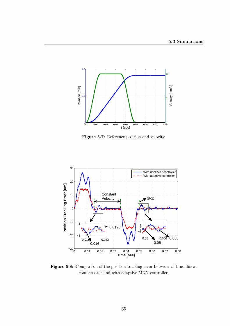
5.3 Simulations

0 0.01 0.02 0.03 0.04 0.05 0.06 0.07 0.080

0.2

0.4

Pos

ition

[mm

]

0 0.01 0.02 0.03 0.04 0.05 0.06 0.07 0.080

5

10

t (sec)

Vel

ocity

[mm

/s]


0 0.01 0.02 0.03 0.04 0.05 0.06 0.07 0.08−30

−20

−10

0

10

20

30

Time [sec]

Po

siti

on

Tra

ckin

g E

rro

r [u

m]

With nonlinear controllerWith adaptive controller

0.016 0.022−4

4

0.05 0.056

−2020.0198

0.016 0.05

Stop

0.055

ConstantVelocity

Figure 5.8: Comparison of the position tracking error between with nonlinear

compensator and with adaptive MNN controller.

65


Items Values

the stage mass 10 kg






0 µm to 400 µm and the initial gap is xg0 = 400 µm. The E-core electromagnetic

constant and parameters of hysteresis operator are set as in Example 1. The

adaptive MNN parameters for the two E/I actuators are the same as in Example

1. The control objective is to make the stage position x follow the reference

position. The reference trajectory is determined by the 3rd order trajectory

planning method [43]. The position and velocity are shown in Figure 5.7. The

trajectory values are shown in table (5.3).

Items Values

the largest displacement 350 µm

the maximum velocity 10 mm/s

the maximum acceleration 1 m/s2

the jerk 200 m/s3

Table 5.3: Trajectory values.

The position tracking errors of control with nonlinear compensator (3.1) and

with adaptive MNN controller (5.3) are shown in Figure 5.8. We define the con-

stant velocity settling time and the stop time as the time instants after which the

position tracking error is less than 1 µm. From the constant velocity segment, it

can be seen that the constant velocity settling time with nonlinear compensator

(0.0198 s) is about 1.22 times longer than of adaptive MNN controller (0.0162 s).

From the stop segment, the stop time with nonlinear compensator (0.055 s) is

about 1.1 times longer than that of adaptive MNN controller (0.05 s). The out-

puts of adaptive MNN controllers are shown in Figure 5.9 and the corresponding

66

5.3 Simulations

0 0.01 0.02 0.03 0.04 0.05 0.06 0.07 0.08−0.5

0

0.5

1

Time [sec]

Ad

apti

ve C

on

tro

ller

Ou

tpu

t [A

]

Adaptive controller 1Adaptive controller 2

0 1 2 3

x 10−3

0

0.1

0.2

Figure 5.9: Outputs of the adaptive controllers.

0 0.01 0.02 0.03 0.04 0.05 0.06 0.07 0.08−15

−10

−5

0

5

10

15

20

25

Time [sec]

Ou

tpu

t F

orc

e [N

]

E/I core 1E/I core 2Net Force

Figure 5.10: Output net force using the adaptive controller.

67


output force of the E/I core actuator 1, E/I core actuator 2 and difference in

Figure 5.10.

5.4 Conclusion

This chapter has proposed a new direct adaptive MNN controller for the reluc-

tance linear actuator with hysteresis. The direct adaptive MNN controller gets

the desired current based on the desired force and actual force using an adaptive

MNN, whose weights are updated using the projection function. Then the adap-

tive MNN controller is applied to a stage having paired E/I core actuator. Due to

the simplicity of the nonlinear control configuration, it has a wider range of ap-

plications. The simulation results show that the proposed method is effective in

over-coming the hysteresis parameter uncertainty and promising in high-precision

control applications.

68

6

Acceleration Feedback in a Stage

Having Paired Reluctance Linear

Actuator with Hysteresis

6.1 Introduction

Conventionally, the positioning control design of a stage falls into two parts: (1)

the actuator dynamics is omitted and the force is designed, (2) the current refer-

ence is computed from the designed force based on their static nonlinear relation

[12]. But it does not consider the effect of hysteresis and parameter uncertainty on

the force accuracy. For the hysteresis compensation, using the inverse hysteresis

model [32] is the most noticeable. Reference [39] proposed an inverse hystere-

sis model and obtained a good performance for the reluctance linear actuator.

However, these methods both need precise hysteresis model, which is generally

complex and hardly to obtain. Owing to its online self-learning ability, the adap-

tive neural network can be used to hysteresis compensation methods proposed

in Chapter 4 and Chapterg 5. However the neural network has a complex

algorithm, so it cannot be easily applied in the real-time digital controller.

Acceleration feedback increases the mass of a system as experienced by dis-

turbance force. Acceleration feedback has been applied to land gears [42] and the

voice coil actuator [5] as an auxiliary to position control. The acceleration feed-

back complemented in an existing position controller for a wafer stage control has

69

6. ACCELERATION FEEDBACK IN A STAGE HAVING PAIREDRELUCTANCE LINEAR ACTUATOR WITH HYSTERESIS

been proposed in [10], which splits the acceleration controller into a forward and

a backward path to create the original process behavior for position controller,

and removes the high-bandwidth requirement.

In this paper, since the hysteresis influence on reluctance actuator is mainly in

the low frequencies [38], by regarding the hysteresis force as a disturbance force, an

acceleration feedback can be designed for the fine stage having paired reluctance

linear actuator with hysteresis. The proposed method can improve the process

sensitivity for low frequencies and remove the high-bandwidth requirement. Fur-

thermore, acceleration feedback implementation in digital controller and control

of the fine stage and coarse stage are discussed. The proposed method does not

need the inverse hysteresis model and can be easily applied in the real time dig-

ital controller. Simulation results show that the proposed method is effective in

overcoming the hysteresis force and promising in precision stage control.

6.2 Acceleration feedback control

6.2.1 Basic idea

Consider the relationship between the force command Fd(d) and output force F

in Figure 3.4, the hysteresis force error Fhys is defined as Fhys = Fd − F . Then

from Figure 3.4, a simplified control scheme is shown in Figure 6.1, in which

the stage transfer function Ps(s) is simplified into two integrators and the fine

stage mass m, ignoring extra dynamics in Ps(s) and the other disturbance force.

From Equation (3.3), if the mass of the fine stage is increased, while keeping

the position control band width equal, we get the same output sensitivity but

an improved process sensitivity. Since a larger mass is generally not expected

for high acceleration control in the fine stage, increasing the virtual mass instead

by the feedback of the acceleration in addition to the position, may improve the

process sensitivity by reducing the influence of the force hysteresis.

6.2.2 Design of acceleration feedback in frequency domain

The idea of acceleration control introduced in [10] is reviewed below. A control

structure using the acceleration feedback method as shown in Figure 6.2 is applied

70


( )sC s

+

+setpoint

position

+-

se sx

Acceleration

feedforward

x

1

s

1

sm

1

s

Acceleration

Velocity

dF F

hysF

Figure 6.1: Simplified virtual control scheme.

to reduce the influence of the hysteresis in paired reluctance linear actuator. It is

better that the position controller does not have any change in process behavior

when the acceleration feedback loop is introduced. So the acceleration loop filter

H1(s) and H2(2) are designed as such that the transfer function from the position

controller output to stage acceleration remains the same, namely 1/ms:

H1(s)/ms

1 +H1(s)H2(s)/ms

=1

ms

. (6.1)

From Equation (6.1), it follows that

H1(s) = 1 +1

ms

Ha(s), (6.2)

H2(s) =Ha(s)

1 +Ha(s)/ms

(6.3)

where Ha(s) = H1(s)H2(s) and the hysteresis force rejection only depends on

Ha(s), which can be designed as a second-order lowpass filter or an integrator.

6.2.3 Acceleration feedback implementation for discretiza-

tion

So far, the acceleration feedback used in paired reluctance actuator is considered

in continuous-time domain. The sampling effects must be taken into account

when the digital controller is applied in reality. Usually, there exits a delay of p

71


1

sm

Acceleration

(s)aH

-

dF F

hysF

1

sm(s)aH

1

sm

1(s)H

2 (s)H

( )sC s

+

+setpoint

position

+

se

x

sx1

s

1

s

Velocity

+

+

+

+

+

Acceleration

feedforward

-

Figure 6.2: Using H1(s) and H2(s) in the acceleration feedback loop.

samples in the process transfer function and a delay of q samples caused by the

acceleration measured. From Equation (6.1), we have:

z−p

msH1(z)

1 + z−(p+q)

msH1(z)H2(z)

=z−p

ms

. (6.4)

The discrete acceleration feedback filter H1(z) and H2(z) corresponding to the

delay p and q can be obtained as:

H1(z) = 1 +z−(p+q)

ms

Ha(z), (6.5)

H2(z) =Ha(z)

1 + z−(p+q)

msHa(z)

. (6.6)

In reality the feedback acceleration am is calculated from the measured posi-

tion xs by a digital double differentiator as well

am = T (z)xs =(1− z−1)2

T 2s

xs, (6.7)

where Ts is the sampling period. A disadvantage of double differentiation is a

possible introduction of noise. Since the closed acceleration loop has a lowpass

72


characteristic, it can reduce the noise. In addition, the least-squared method

function used as filter may also reduce the noise impact [9].

From Figure 6.2, an original discrete form of acceleration feedback is shown in

Figure 6.3. However, the acceleration feedforward signal will pass the increased

order system caused by the acceleration feedback instead of passing through Ps(z).

This results in an increased position settling error compared to the situation with-

out acceleration feedback [10]. Instead of increasing the feedforward order to cope

with the process dynamics for reducing the position settling error, we shift the

feedforward entry point towards the force command input into the acceleration

feedback loop as shown in Figure 6.4. However, the feedforward force now enters

the system loop at the same point as the hysteresis force. To avoid this problem,

a relative acceleration is used by the deviation between the acceleration feedfor-

ward and the acceleration feedback [10]. A delay of p + q samples must be used

to match the acceleration feedback delay from the acceleration feedforward, and

define M(z) = z−(p+q)

ms.

6.2.4 Acceleration feedback in a fine stage connected to a

coarse stage

The practical reluctance linear actuator has a moving rang of only about 1mm,

which is insufficient for the stage in the lithographic equipment. This problem is

solved by introducing a coarse stage actuated by the linear motor [8], which can

travel over large distances with moderate micrometer-rang accuracy, and moves

the fine stage actuated by the reluctance linear actuator [12]. Usually the E/I

core part is connected to the coarse stage to avoid crossover of cables and cooling

hoses to the accurate fine stage.

Based on Figure 6.3, a totally basic control scheme which combines the fine

stage and coarse stage controllers with acceleration feedback loop is shown in

Figure 6.5. Since the fine stage has a key roll in the final position accuracy, the

acceleration feedback is added into the fine stage control loop. In Figure 6.5,

Pl(z) represents the coarse stage process system. The coarse stage is required to

track the fine stage to keep the E/I core and fine stage close together. To this

end, the gap sensors measure the gap distance between the coarse stage and fine

73


( )sC z+

setpoint

position

+-

se sx

( )T z

( )1H z

( )2H z

-

++

Acceleration

feedforward

( )sP zdF F

hysF

ma

Figure 6.3: Discrete form of acceleration feedback.

( )sC z+

setpoint

position

+-

se sx

( )T z

( )M z

( )1H z

( )2H z

-

+

+

+

-

Acceleration

feedforward

( )sP zdF F

hysF

ma

Figure 6.4: The final discrete form of acceleration feedback.

stage by the “gd”signal. As the fine stage is decoupled from the coarse stage by

tracking the interferometer, the coarse stage controller Cl(z) is designed for the

dynamics of the coarse stage without taking the fine stage into account. In the

feedforward path, since a reaction force is added to the coarse stage while the

fine stage accelerates, the mass of the fine stage must be included to accelerate

the coarse stage.

6.3 Simulations

In order to verify whether the proposed acceleration feedback configuration can be

applied in high-precision systems, we do the following simulations on the scheme

as shown in Figure 6.5. For comparison, the no acceleration feedback case is used.

74

6.3 Simulations

gd

+s lm m

( )lP z

+

+( )lC z

+-

-

le l

x

( )sC z

+setpoint

position

+-

sm

se

FD

NC1

NC2

( )sP z

EI1

EI2

+

-

sx

Acceleration

feedforwarda

x

dF F

1dF

2dF

1i

2i

( )T z1F

2F

+

( )T z

( )M z

( )1H z

( )2H z

-

+

+-

ma

Figure 6.5: Total feedback scheme for coarse stage and fine stage using

acceleration feedback.

The reluctance linear actuator with hysteresis is modeled by Equation (2.80),

whose parameters are chosen as in the patent [80] and shown in table (6.1).

Items Values




the hysteresis operator parameters λ1 = 0.02 and λ2 = 10


The gaps xg1 and xg2 between the E-core 1,2 and the stage are in the range

of 0 µm to 400 µm and the initial gap is xg0 = 400 µm. The stage parameters

are shown in table (6.2).

A typical setpoint position profile [8], which is used during exposing in litho-

graphic equipment, is determined by the 3rd order trajectory planning method

[43]. The position and velocity are shown in Figure 6.6, the scanning velocity

settling time is defined as the time instants after which the position tracking er-

ror is less than 10 nm . The scanning velocity is 0.25 m/s, the acceleration is

75


Items Values

the fine stage mass 10 kg

the coarse stage mass 20 kg






10 m/s2.

In the practical application, the position controller is designed as a PI+lead

compensator, which makes the position-controlled fine stage system having about

a 100 Hz bandwidth corresponding the mechanical structure. The acceleration

feedback filters H1(z) and H2(z) are designed as follows. Hz(z) is chosen as

an integrator with a gain that creates a closed acceleration loop bandwidth of

fabw = 130Hz, leading to

Ha(z) =2πmsfabwTs

1− z−1. (6.8)

By assuming that the process delay is p = 1 and the acceleration measurement

delay is q = 1, then M(z) = z−2/ms. From Equation (6.5) and Equation (6.6),

it follows that

H1(z) = 1 +2πfabwTs

1− z−1z−2, (6.9)

H2(z) =2πmsfabwTs

1− z−1 + 2πfabwTsz−2. (6.10)

The control objective is to make the stage position xs follow the reference

position x and have a quick scanning velocity settling time. Figure 6.7 shows the

position tracking errors with and without acceleration feedback. The scanning

velocity settling time is about 56 ms without acceleration feedback slower than

with acceleration feedback 46 ms.

Figure 6.8 shows the fine stage position loop process sensitivity. we define

the transfer function following Equation (3.3), which is added to the real force

F as shown in Figure 6.5. From Figure 6.8, the fine stage position loop process

76

6.3 Simulations

0 0.05 0.1 0.15 0.2 0.25 0.3 0.35 0.4−0.02

−0.01

0

0.01

0.02

0.03

0.04

0.05

0.06

Po

siti

on

[m

]

Time [sec]

Setpoint positionVelocity/10Acceleration/500

settling time


0 0.05 0.1 0.15 0.2 0.25 0.3 0.35 0.4−2

−1

0

1

2x 10

−5

Po

siti

on

Err

or[

m]

0.08 0.1 0.12 0.14 0.16 0.18−1

−0.5

0

0.5

1x 10

−7

Time [sec]

Po

siti

on

Err

or[

m]

No acc. FeedbackAcc. Feedback


0.71s

0.81s

Figure 6.7: Position tracking error.

77


100

101

102

103

−300

−280

−260

−240

−220

−200

−180

−160

−140

−120

−100

Frequency [Hz]

Mag

nit

ud

e [d

B]


Figure 6.8: Position loop process sensitivity of the fine stage.

100

101

102

103

−90

−80

−70

−60

−50

−40

−30

−20

−10

0

10

Frequency [Hz]

Mag

nit

ud

e [d

B]

Fine stage closed loop bode plot

No acc. feedbackAcc. feedback

Figure 6.9: Fine stage closed control loop bode plots.

78

6.4 Comparison of the proposed hysteresis compensation methods

100

101

102

103

−90

−80

−70

−60

−50

−40

−30

−20

−10

0

10

Frequency [Hz]

Mag

nit

ud

e [d

B]

Coarse stage closed loop bode plot

No acc. feedbackAcc. feedback

Figure 6.10: Coarse stage closed control loop bode plots.

sensitivity without acceleration feedback is about −170 dB and with acceleration

feedback decreases to about −230 dB for low frequencies. It is clear that, the

acceleration feedback introduced into the system provides a low process sensitivity

for the hysteresis force.

The closed control loop bode plots of the fine stage with and without accel-

eration feedback are shown in Figure 6.9. It can be seen that, the acceleration

feedback loop added into the system loop does not change the fine stage close

loop for low frequencies, the magnitude increases a little at high frequencies. And

closed control loop bode plots of the coarse stage with and without acceleration

feedback is shown in Figure 6.10.

6.4 Comparison of the proposed hysteresis com-

pensation methods

In the following, the comparison for the performance of the proposed hysteresis

compensation methods in Chapter 4 -6 will be discussed by the simulations.

79


0 2000 4000 6000 8000 10000−0.4

−0.3

−0.2

−0.1

0

0.1

0.2

0.3

0.4

Time

Fo

llow

ing

fo

rce

erro

r [N

]

MNN compensatorDirect MNN

Figure 6.11: Comparison of the force following error.

Example 1 : A simulation for the current-driven reluctance linear actuator is con-

ducted to verify the performance of the proposed adaptive MNN compensator

shown in Figure 4.1 in Chapter 4. For comparison the direct adaptive MNN

shown in Figure 5.1 in Chapter 5. In this simulation, the reluctance actuator

parameters and the adaptive MNN compensator parameters are selected as in

Chapter 4 simulation Example 1. The parameters for the direct adaptive MNN

compensation method proposed in Chapter 5 are selected as in Chapter 5 simula-

tion example 1. The control objective is to make the system output F following

the reference force Fd. A reference force depicted in Figure 5.3.

The comparison of the following force errors with adaptive MNN compensator

proposed in Chapter 4 and direct adaptive MNN proposed in Chapter 5 is shown

in Figure 6.11. We can find that the following force error with adaptive MNN

compensator proposed in Chapter 4 has a smaller following force error and a

quicker convergence time than the direct adaptive MNN proposed in Chapter 5.

The main reason for difference of the following force error is that the nonlinear

compensator is used in Chapter 4. Example 2 : In order to verify the performance

80

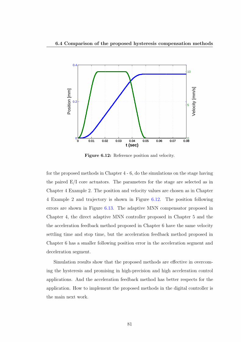
6.4 Comparison of the proposed hysteresis compensation methods

0 0.01 0.02 0.03 0.04 0.05 0.06 0.07 0.080

0.2

0.4P

ositi

on [m

m]

0 0.01 0.02 0.03 0.04 0.05 0.06 0.07 0.080

5

10

t (sec)

Vel

ocity

[mm

/s]


for the proposed methods in Chapter 4 - 6, do the simulations on the stage having

the paired E/I core actuators. The parameters for the stage are selected as in

Chapter 4 Example 2. The position and velocity values are chosen as in Chapter

4 Example 2 and trajectory is shown in Figure 6.12. The position following

errors are shown in Figure 6.13. The adaptive MNN compensator proposed in

Chapter 4, the direct adaptive MNN controller proposed in Chapter 5 and the

the acceleration feedback method proposed in Chapter 6 have the same velocity

settling time and stop time, but the acceleration feedback method proposed in

Chapter 6 has a smaller following position error in the acceleration segment and

deceleration segment.

Simulation results show that the proposed methods are effective in overcom-

ing the hysteresis and promising in high-precision and high acceleration control

applications. And the acceleration feedback method has better respects for the

application. How to implement the proposed methods in the digital controller is

the main next work.

81


0 200 400 600 800 1000 1200 1400 1600−30

−20

−10

0

10

20

30

Time

Fo

llow

ing

err

or

[N]

Acceleration FeedbackMNN compensatorDirect MNN

Figure 6.13: Comparison of the position tracking error.

6.5 Conclusion

This chapter has proposed a new acceleration feedback control method for the

fine stage having paired reluctance linear actuator with hysteresis. By consid-

ering the fine stage force error caused by the hysteresis in the reluctance linear

actuator, as a disturbance force and since the main hysteresis influence is in the

low frequencies, the acceleration feedback loop can be design. The practical im-

plementation has been discussed for the digital controller. The simulation results

show that by properly choosing H1 and H2, the acceleration feedback can provide

a low process sensitivity and a fast scanning velocity settling time. The proposed

method is effective in overcoming the reluctance linear actuator with hysteresis

and promising in high-precision control applications.

82

7

Conclusions

In this thesis, we introduce the thesis background, the challenge to the next-

generation fine stage actuator and the main contributions in Chapter 1. In

order to study the reluctance actuator, the models without hysteresis for the C-

core and E-Core reluctance actuators are reviewed and the models with hysteresis

for the C-core and E-Core reluctance actuators are proposed in Chapter 2. The

reluctance models and the basic control method that introduced in Chapter 3

are the basic for this thesis works.

The main existing compensation methods for the reluctance actuator with

hysteresis usually uses the inverse hysteresis models, which is complex and not

easily to be implement. Owing to the online self-learning and estimation capa-

bility of the neural network, a hysteresis current compensation configuration for

the reluctance actuator with hysteresis based on the adaptive multi-layer neural

network is proposed in Chapter 4. The main contributions of this method is

a hysteresis compensator for current-driven reluctance linear actuator using the

adaptive MNN proposed for the first time and the inverse hysteresis model is not

used.

Although the compensation method proposed in Chapter 4 may reduce the

influence caused by the hysteresis on the reluctance force, the reluctance model is

also used. A new nonlinear control method is proposed for the stage having paired

reluctance linear actuator with hysteresis using the direct adaptive neural network

is proposed in Chapter 5. The main advantage of the proposed adaptive MNN

83

7. CONCLUSIONS

controller is that the reluctance linear actuator model and the inverse hysteresis

model are not required.

The compensation methods proposed in Chapter 4 and Chapter 5 are both

used the adaptive MNN, but the complex structure and algorithm are difficultly

implemented in the digital controller now. The acceleration feedback for the

fine stage having paired reluctance linear actuator with hysteresis is designed in

Chapter 6. The feature of this method lies in that by considering the hysteresis

force as a disturbance force to design the acceleration feedback loop to reduce the

influence of the hysteresis force. The proposed method can improve the process

sensitivity for low frequencies and remove the high-bandwidth requirement. This

acceleration feedback method could easily implemented in the digital controller.

Simulation results show that the proposed methods are effective in overcom-

ing the hysteresis and promising in high-precision and high acceleration control

applications. And the acceleration feedback method has better respects for the

application. How to implement the proposed methods in the digital controller is

the main next work.

84

References

[1] M. Al Janaideh, Feng Ying, S. Rakheja, Su Chun-Yi, and C. A. Rab-

bath. Hysteresis compensation for smart actuators using inverse generalized

prandtl-ishlinskii model. In American Control Conference, 2009. ACC ’09.,

pages 307–312, 2009. 43

[2] J. S. Albus. A new approach to manipulator control: the cerebellar model

articulation controller (cmac). Journal of Dynamic Systems, pages 220–227,

1975. 44

[3] A. Alessandri and T. Parisini. Nonlinear modeling of complex large-scale

plants using neural networks and stochastic approximation. IEEE Trans-

actions on Systems, Man and Cybernetics, Part A: Systems and Humans,

27(6):750–757, 1997. 45

[4] B Appelbe. Rate independent hysteresis in terrestrial hydrology. IEEE

Control Systems, 29(1):44–69, 2009. 16

[5] A. Babinski and Tsao Tsu-Chin. Acceleration feedback design for voice coil

actuated direct drive. In American Control Conference, 1999. Proceedings

of the 1999, volume 5, pages 3713–3717 vol.5, 1999. 69

[6] Giorgio Bertotti. Hysteresis in magnetism: for physicists, materials scien-

tists, and engineers. Academic press, 1998. 11, 19

[7] H. Butler. Scanning stage technology for exposure tools. Microlithogr, 8(2):8–

16, 1999. 4

85

REFERENCES

[8] H. Butler. Position control in lithographic equipment. IEEE Control Sys-

tems, 31(5):28–47, 2011. 2, 3, 5, 6, 7, 8, 38, 73, 75

[9] H. Butler. Adaptive feedforward for a wafer stage in a lithographic tool.

IEEE Transactions on Control Systems Technology, PP(99):1–7, 2012. 47,

73

[10] Hans Butler. Acceleration feedback in a lithographic tool. Control Engineer-

ing Practice, 20(4):453–464, 2012. 70, 73

[11] A. Cavallo, C. Natale, S. Pirozzi, and C. Visone. Effects of hysteresis com-

pensation in feedback control systems. IEEE Transactions on Magnetics,

39(3):1389–1392, 2003. 11

[12] Ping-Wei Chang. E/i core actuator commutation formula and control

method, 2007. 40, 50, 51, 60, 69, 73

[13] V. Cherkassky, D. Gehring, and F. Mulier. Comparison of adaptive meth-

ods for function estimation from samples. IEEE Transactions on Neural

Networks, 7(4):969–984, 1996. 44, 45

[14] R. M. Corless, G. H. Gonnet, D. E. G. Hare, D. J. Jeffrey, and D. E.

Knuth. On the lambertw function. Advances in Computational Mathematics,

5(1):329–359, 1996. 17

[15] G. Cybenko. Approximation by superpositions of a sigmoidal function. Math-

ematics of Control, Signals and Systems, 2(4):303–314, 1989. 44

[16] A. M. Dabroom and H. K. Khalil. Output feedback sampled-data control of

nonlinear systems using high-gain observers. IEEE Transactions on Auto-

matic Control, 46(11):1712–1725, 2001. 45

[17] Avinash Dixit. Hysteresis, import penetration, and exchange rate pass-

through. The Quarterly Journal of Economics, pages 205–228, 1989. 16

[18] A. A. Eielsen, J. T. Gravdahl, and K. Y. Pettersen. Adaptive feed-

forward hysteresis compensation for piezoelectric actuators. Rev Sci Instrum,

83(8):085001, 2012. 11

86

REFERENCES

[19] James Alfred Ewing. On the production of transient electric currents in iron

and steel conductors by twisting them when magnetised or by magnetising

them when twisted. Proceedings of the Royal Society of London, 33(216-

219):21–23, 1881. 15

[20] Lin Faa-Jeng, Shieh Hsin-Jang, and Huang Po-Kai. Adaptive wavelet neural

network control with hysteresis estimation for piezo-positioning mechanism.

IEEE Transactions on Neural Networks, 17(2):432–444, 2006. 43, 57

[21] Chen Fu-Chuang and H. K. Khalil. Adaptive control of a class of nonlinear

discrete-time systems using neural networks. IEEE Transactions on Auto-

matic Control, 40(5):791–801, 1995. 44

[22] Kenchi Funahashi. On the approximate realization of continuous mappings

by neural networks. Neural Networks, 2(3):183–192, 1989. 44, 45

[23] William S Galinaitis and Robert C Rogers. Control of a hysteretic actuator

using inverse hysteresis compensation. In 5th Annual International Sym-

posium on Smart Structures and Materials, pages 267–277. International

Society for Optics and Photonics, 1998. 16

[24] S. S. Ge, C. C. Hang, and Zhang Tao. Adaptive neural network control

of nonlinear systems by state and output feedback. IEEE Transactions on

Systems, Man, and Cybernetics, Part B: Cybernetics, 29(6):818–828, 1999.

45

[25] S. S. Ge, C. C. Hang, and T. Zhang. Nonlinear adaptive control using neural

networks and its application to cstr systems. Journal of Process Control,

9(4):313–323, 1999. 45

[26] S S Ge, Chang C Hang, Tong H Lee, and Tao Zhang. Stable adaptive neural

network control. Springer Publishing Company, Incorporated, 2010. 57, 58

[27] S. S. Ge and C. Wang. Adaptive control of uncertain chua’s circuits. IEEE

Transactions on Circuits and Systems I: Fundamental Theory and Applica-

tions, 47(9):1397–1402, 2000. 45

87

REFERENCES

[28] C. J. Goh. Model reference control of non-linear systems via implicit function

emulation. Int. J. Control, 60(90-115), 1994. 44

[29] J. Q. Gong and Yao Bin. Adaptive robust control without knowing bounds

of parameter variations. In Decision and Control, 1999. Proceedings of the

38th IEEE Conference on, volume 4, pages 3334–3339 vol.4, 1999. 48

[30] William B Haines. Studies in the physical properties of soil. v. the hysteresis

effect in capillary properties, and the modes of moisture distribution asso-

ciated therewith. The Journal of Agricultural Science, 20(01):97–116, 1930.

15

[31] Kurt Hornik, Maxwell Stinchcombe, and Halbert White. Multilayer feedfor-

ward networks are universal approximators. Neural Networks, 2(5):359–366,

1989. 44

[32] R. V. Iyer and Tan Xiaobo. Control of hysteretic systems through inverse

compensation. IEEE Control Systems, 29(1):83–99, 2009. 11, 43, 69

[33] R. V. Iyer and Tan Xiaobo. Control of hysteretic systems through inverse

compensation. IEEE Control Systems, 29(1):83–99, 2009. 11

[34] Ram V Iyer and Matthew E Shirley. Hysteresis parameter identification with

limited experimental data. IEEE Transactions on Magnetics, 40(5):3227–

3239, 2004. 16

[35] L. Jin, P. N. Nikiforuk, and M. M. Gupta. Direct adaptive output track-

ing control using multilayered neural networks. IEEE Proceedings Control

Theory and Applications, 140(6):393–398, 1993. 44

[36] Oh Jinhyoung, B. Drincic, and D. S. Bernstein. Nonlinear feedback models

of hysteresis. IEEE Control Systems, 29(1):100–119, 2009. 43

[37] Oh Jinhyoung, B. Drincic, and Bernstein D S. Nonlinear feedback models of

hysteresis. IEEE Control Systems, 29(1):100–119, 2009. 16

88

REFERENCES

[38] A. Katalenic, J. de Boeij, H. Butler, and P. P. J. van den Bosch. Lineariza-

tion of a current-driven reluctance actuator with hysteresis compensation.

Mechatronics, 23(2), 2013. 11, 70

[39] Boeij J. Katalenic A. Linearization of the reluctance force actuator based on

the parametric hysteresis inverse and a 2d spline. In Proceedings of the 8th

International Symposium on Linear Drives for Industry Applications (LDIA

2011), 2011. 16, 19, 41, 43, 69

[40] Pavel Krejci and Vladimir Lovicar. Continuity of hysteresis operators in

sobolev spaces. Aplikace matematiky, 35(1):60–66, 1990. 16

[41] Klaus Kuhnen. Modeling, identification and compensation of complex hys-

teretic nonlinearities: A modified prandtl ishlinskii approach. European

Journal of Control, 9(4):407–418, 2003. 16

[42] Seung-Keon Kwak, Gregory Washington, and Rama K Yedavalli. Acceler-

ation feedback-based active and passive vibration control of landing gear

components. Journal of Aerospace Engineering, 15(1):1–9, 2002. 69

[43] Paul Lambrechts, Matthijs Boerlage, and Maarten Steinbuch. Trajectory

planning and feedforward design for electromechanical motion systems. Con-

trol Engineering Practice, 13(2):145–157, 2005. 52, 66, 75

[44] K. K. Leang and S. Devasia. Iterative feedforward compensation of hysteresis

in piezo positioners. In Proceedings. 42nd IEEE Conference on Decision and

Control, 2003, volume 3, pages 2626–2631 Vol.3, 2003. 16

[45] K K Leang, Zou Qingze, and S. Devasia. Feedforward control of piezoactua-

tors in atomic force microscope systems. IEEE Control Systems, 29(1):70–82,

2009. 16

[46] A. U. Levin and K. S. Narendra. Control of nonlinear dynamical systems

using neural networks. ii. observability, identification, and control. IEEE

Transactions on Neural Networks, 7(1):30–42, 1996. 44

89

REFERENCES

[47] Yu-Ping Liu, Kang-Zhi Liu, and Xiaofeng Yang. A direct adaptive mnn

control method for stage having paired reluctance linear actuator with hys-

teresis. Intelligent Control and Automation, 5(04):213, 2014. 12, 57

[48] Yu-Ping Liu, Kang-Zhi Liu, and Xiaofeng Yang. Nonlinear current control

for reluctance actuator with hysteresis compensation. Journal of Control

Science and Engineering, 4, 2014. 12

[49] Yuping Liu, Lianfei ZHAI, and Tianyou Chai. Nonlinear adaptive pid control

using neural networks and multiple models and its application. Journal of

Chemical Industry and Engineering (China), 7:013, 2008. 43, 44, 57

[50] Erwin Madelung. Uber magnetisierung durch schnellverlaufende strome und

die wirkungsweise des rutherford marconischen magnetdetektors. Annalen

der Physik, 322(10):861–890, 1905. 15

[51] I. Mayergoyz. Mathematical Models of Hysteresis. New York: SpringerVerlag,

1991. 16

[52] John C. McCallum. Historical cost of computer memory and storage, 2013.

8, 9

[53] Chen Min and C. R. Knospe. Feedback linearization of active magnetic bear-

ings: current-mode implementation. IEEE/ASME Transactions on Mecha-

tronics, 10(6):632–639, 2005. 11

[54] S. Mittal and C. H. Menq. Hysteresis compensation in electromagnetic ac-

tuators through preisach model inversion. IEEE/ASME Transactions on

Mechatronics, 5(4):394–409, 2000. 11

[55] S. Mittal and C. H. Menq. Hysteresis compensation in electromagnetic ac-

tuators through preisach model inversion. IEEE/ASME Transactions on

Mechatronics, 5(4):394–409, 2000. 43

[56] G. E. Moore. Cramming more components onto integrated circuits. Electron.

Mag., 38(8):4–7, 1965. 9

90

REFERENCES

[57] P. E. Moraal and J. W. Grizzle. Observer design for nonlinear systems

with discrete-time measurements. IEEE Transactions on Automatic Control,

40(3):395–404, 1995. 45

[58] van Eijk J. Munnig Schmidt S., Schitter G. The design of high performance

mechatronics. Delft University Press, Netherlands, 2011. 1, 2, 4

[59] K. S. Narendra and S. Mukhopadhyay. Adaptive control of nonlinear mul-

tivariable systems using neural networks. In Proceedings of the 32nd IEEE

Conference on Decision and Control, 1993, volume 4, pages 3066–3071, 1993.

44

[60] K. S. Narendra and K. Parthasarathy. Identification and control of dynamical

systems using neural networks. IEEE Transactions on Neural Networks,

1(1):4–27, 1990. 44

[61] San Phyo Phyo, Ren Beibei, S. S. Ge, Lee Tong-Heng, and Liu Jin-Kun.

Adaptive neural network control of hard disk drives with hysteresis friction

nonlinearity. IEEE Transactions on Control Systems Technology, 19(2):351–

358, 2011. 43, 57

[62] W. S. McCulloch Pitts and W. A logical calculus of the ideas immanent in

nervous activity. Bull. Math. biophys, 5:115–133, 1943. 44, 45

[63] M. Krasnoselskii Pokrovskii and A. M. Krasnoselskii and A. Pokrovskii. New

York: Springer-Verlag, 1989. 16

[64] M. M. Polycarpou and P. A. Ioannou. Learning and convergence analysis of

neural-type structured networks. IEEE Transactions on Neural Networks,

3(1):39–50, 1992. 44

[65] F. Preisach. Uber die magnetische nachwirkung. Zeitschrift fur Physik,

94(5-6):277–302, 1935. 15

[66] ASML Products. Pas 5500/100d, i-line stepper, 2014. 3

[67] ASML Products. Pas 5500/1150c, 193-nm step-and-scan, 2014. 5

91

REFERENCES

[68] ASML Products. Twinscan nxe:3300b, 2014. 6, 7

[69] D. Psaltis, A. Sideris, and A. A. Yamamura. A multilayered neural network

controller. IEEE Control Systems Magazine, 8(2):17–21, 1988. 44

[70] D E Rumelhart. Learning internal representations by error propagation.

Parallel Distributed Processing, 1(362-378), 1986. 44

[71] N. Sadegh. A perceptron network for functional identification and control

of nonlinear systems. IEEE Transactions on Neural Networks, 4(6):982–988,

1993. 44, 45

[72] Andre M. Shaw and Francis J. Doyle Iii. Multivariable nonlinear control

applications for a high purity distillation column using a recurrent dynamic

neuron model. Journal of Process Control, 7(4):255–268, 1997. 45

[73] Ralph C Smith. Smart material systems: model development, volume 32.

Siam, 2005. 16

[74] G. Song, Zhao Jinqiang, Zhou Xiaoqin, and J. A. De Abreu-Garcia. Tracking

control of a piezoceramic actuator with hysteresis compensation using inverse

preisach model. IEEE/ASME Transactions on Mechatronics, 10(2):198–209,

2005. 16

[75] M. Brokate Sprekels and J. Hysteresis and Phase Transitions. New York:

Springer-Verlag, 1996. 16

[76] Fu-Chun Sun, Han-Xiong Li, and Lei Li. Robot discrete adaptive control

based on dynamic inversion using dynamical neural networks. Automatica,

38(11):1977–1983, 2002. 45

[77] Xiaobo Tan and John S. Baras. Modeling and control of hysteresis in mag-

netostrictive actuators. Automatica, 40(9):1469–1480, 2004. 16

[78] Gang Tao and Petar V Kokotovic. Adaptive control of systems with actuator

and sensor nonlinearities. John Wiley Sons, Inc., 1996. 16

92

REFERENCES

[79] Intel technology news. Toshiba starts mass production of world’s first 15nm

nand flash memorie, 2014. 9

[80] Ting-Chien Teng and Bausan Yuan. Stage having paired e/i core actuator

control, 2000. 38, 39, 61, 75

[81] A. T. Vemuri and M. M. Polycarpou. Neural-network-based robust fault

diagnosis in robotic systems. IEEE Transactions on Neural Networks,

8(6):1410–1420, 1997. 45

[82] A. T. Vemuri, M. M. Polycarpou, and S. A. Diakourtis. Neural network based

fault detection in robotic manipulators. IEEE Transactions on Robotics and

Automation, 14(2):342–348, 1998. 45

[83] Augusto Visintin. Differential models of hysteresis, volume 1. Springer

Berlin, 1994. 15

[84] J. W. Vrijsen, N. H. Jansen. Comparison of linear voice coil and reluctance

actuators for high-precision applications. In 2010 14th International Power

Electronics and Motion Control Conference (EPE/PEMC), pages S3–29–S3–

36, 2010. 10

[85] C. Wang and S. S. Ge. Adaptive synchronization of uncertain chaotic systems

via backstepping design. Chaos, Solitons Fractals, 12(7):1199–1206, 2001. 45

[86] Smith F W Widrow B. Pattern-recognizing control systems. Computer and

Information Sciences (COINS) Proceedings, 1964. 44

[87] Qingsong Xu and Yangmin Li. Dahl model-based hysteresis compensation

and precise positioning control of an xy parallel micromanipulator with piezo-

electric actuation. Journal of Dynamic Systems, Measurement, and Control,

132(4):041011, 2010. 43

[88] X. Xue and J. Tang. Robust and high precision control using piezoelectric

actuator circuit and integral continuous sliding mode control design. Journal

of Sound and Vibration, 293(1-2):335–359, 2006. 11

93

REFERENCES

[89] Liu Yu-Ping, Liu Kang-Zhi, and Yang Xiaofeng. Hysteresis compensation

control for reluctance actuator force using neural network. In 2013 32nd

Chinese Control Conference (CCC), pages 3354–3359, 2013. 57

[90] T. Zhang. Neural-based direct adaptive control for a class of general non-

linear systems. International Journal of Systems Science, 28(10):1011–1020,

1997. 45

94

List of Publications

International Journal Papers

• Yu-Ping Liu, Kang-Zhi Liu, and Xiaofeng Yang, (2014) Non-

linear Current Control for Reluctance Actuator with Hysteresis

Compensation, Journal of Control Science and Engineering, vol.

2014.

• Liu, Y. P., Liu, K. Z., Yang, X. (2014). A Direct Adaptive

MNN Control Method for Stage Having Paired Reluctance Lin-

ear Actuator with Hysteresis. Intelligent Control and Automa-

tion, 5(04), 213.

International Conference Papers

• Yu Ping Liu, kang Zhi Liu and Xiaofeng Yang, (2014) Hysteresis

Compensation Control for a Current-driven Reluctance Actua-

tor Using the Adaptive MNN. Applied Mechanics and Materials,

643, 60.

• Liu, Y. P., Liu, K. Z., Yang, X. (2013). Hysteresis compensation

control for reluctance actuator force using neural network. In

Control Conference (CCC), 2013 32nd Chinese (pp. 3354-3359).

Nonlinear Control Methods for Reluctance Actuator with ...

Documents

Transcript of Nonlinear Control Methods for Reluctance Actuator with ...