Nonlinear Analysis of a Single Stage Pressure Relief Valve · 2009-11-10 · Nonlinear Analysis of...

Nonlinear Analysis of a Single Stage Pressure Relief

Valve

Gábor Licskó ∗ Alan Champneys † Csaba Hős ‡

Abstract—A mathematical model is derived that

describes the dynamics of a single stage relief valve

embedded within a simple hydraulic circuit. The aim

is to capture the mechanisms of instability of such

valves, taking into account both fluid compressibil-

ity and the chattering behaviour that can occur when

the valve poppet impacts with its seat. The initial

Hopf bifurcation causing oscillation is found to be ei-

ther super- or sub-critical in different parameter re-

gions. For flow speeds beyond the bifurcation, the

valve starts to chatter, a motion that survives for a

wide range of parameters, and can be either periodic

or chaotic. This behaviour is explained using recent

theory of nonsmooth dynamical systems, in particu-

lar an analysis of the grazing bifurcations that occur

at the onset of impacting behaviour.

Keywords: relief valve, chaos, grazing, piecewise-

smooth

1 Instabilities in relief valves

Hydraulic relief valves are widely used to limit pressurein hydraulic power transmission and control systems.There is a rich literature that describes their usage in hy-draulic circuits and gives information on their design andapplication. A brief overview on elements of hydraulicsystems can be found in the book of Bolton [1]. Moredetailed information on hydraulic elements can be foundin Steward’s book [10] together with lots of industrialexamples mostly from the area of manufacturing. Kay[8] focuses more on industrial pneumatics again withmany application examples.

In hydraulic circuits that are in steady operating condi-tions, and the constant flow rate input of the system isless than the delivered flow rate of the pump then thedifference will flow through the by-pass line secured bya relief valve. Such situations arise when economic op-eration is not so important. The other case when reliefvalves interact in most of the hydraulic equipments (suchas those installed on excavators, etc.) is when transient

∗Department of Applied Mechanics, Budapest University ofTechnology and Economics, [email protected]

†Department of Engineering Mathematics, University of Bristol,[email protected]

‡Department of Hydrodynamic Systems, Budapest University ofTechnology and Economics, [email protected]

phenomena occur (e.g. the scoop sticks in a rocky layerbelow the soil) and the pressure rises much above the tol-erable limit. The relief valve has to intervene and limitthe pressure so that other parts of the circuit are notdamaged. These are the main reasons why designers ofsuch systems have to insert pressure limitters into thecircuit.Figure 1 shows a so called direct operated pressure relief

valve. The simplest configuration of such a relief valveis when an orifice is closed by a poppet or similar ele-ment. The closing force can be adjusted by pre-stressinga spring that presses the poppet towards the valve seat.This force divided by the cross-sectional area of the ori-fice also represents the opening pressure, the treshold atwhich the safety valve will come into operation.There are numerous examples in industry where thesekinds of valves can vibrate when their equilibria lose sta-bility and many researchers have been interested in theinvestigation of this phenomenon. As far back as the1960’s researchers suspected that the piping to and fromthe relief valve cannot be neglected. Kasai [7] carriedout a very detailed investigation of a simple poppet valveand he deduced a stability criterion analytically. He alsoproposed that circumstances other than just nonlinear-ity such as the poppet geometry or the change in the oiltemperature can also lead to stability loss. Moreover heperformed experiments and found good coincidence withhis analytical results. Thomann [11] was also interestedin the analysis of a pipe-valve system. He used a sim-ple poppet type valve but analysed how different poppetgeometries affect the stability. He investigated a conical

Figure 1: Direct operated pressure relief valve (1- valve housing; 2 - spring; 4 - poppet; 5 - ad-justing wheel; P - inlet; T - outlet) (image source:http://www.boschrexroth.com/).

IAENG International Journal of Applied Mathematics, 39:4, IJAM_39_4_12______________________________________________________________________________________

(Advance online publication: 12 November 2009)

and a cylindrical poppet together with conical or cylin-drical seats, and their combination. Hayashi et al.[5, 6],built up a model with a constant supply pressure and in-vestigated the valve’s response and stability, finding thata Hopf bifurcation occurs.

This report shall consider a modern analysis of reliefvalve chatter using ideas from nonsmooth dynamicalsystems. See e.g. [2]. A simple set-up will be chosenthat considers the dynamics of the valve in the contextof a hydraulic circuit.The rest of the work is organized as follows: firstin Section 2 we present a mathematical model thatis believed to accurately describe the behaviour of apressure relief valve. In Subsection 2.2 we continue witha linear stability analysis of the derived equations andtry to show that in certain cases self-excited limit cyclevibration occur. In Subsection 2.3 we carry out a nonlin-ear analysis, since we wish to determine the stability ofthe limit cycle found. We will also be interested in thepossible change of this stability by varying parametersalong the critical curve where dynamical stability lossoccurs.Exciting nonsmooth phenomena can be exhibited bythese kinds of mechanical systems when moving partscollide with standing ones. Such impacts can affect thesystem’s behaviour globally and we wish to understandmore about how nonsmooth bifurcations occur in thisparticular example (e.g. grazing bifurcation). Towardsthis we will use numerical techniques in Section 3 andcompute bifurcation diagrams using an appropriate sim-ulator. Then in Section 4 we will also try to investigatethe dynamics of grazing analytically.

2 The mathematical model

Figure 2 depicts a sketch of the analyzed system, whichis similar to those used by Kasai [7] and Hayashi [6].The system consists of a hydraulic aggregate and a safetyvalve connected by fluid conveying tubes, the fluid is redi-rected into an oil chamber after leaving the test valve.The oil is supplied by an aggregate that consist of thegear pump and an additional safety valve for the protec-tion of the system. This hydraulic aggregate provides thesystem the flow rate Qp. However, due to compressibil-ity of the fluid and elasticity of the tubes, the flow rateat the test valve can be different from that one at theexit to the pump. To model the compressibility effects, ahypothetical chamber is added whose volume is equal tothe total volume of oil in the system. This chamber willrepresent the stiffness of our system.The mass balance equation for this chamber (labeled 3 inFig. 2) can be written as follows:

d

dt(ρV ) = ρ [Qp − Q (x, p)] , (1)

��

��

��

��

��

��

��

��

��

Aggregate

V ,

Test valve

1

2

3

4

5

p

s k

m

Qp

Q(x, p)

0

x

Figure 2: Schematic diagram of a simple hydraulic sys-tem consisting of a gear pump (1), a relief valve (2), ahypothetical chamber (3) that represents the total tub-ing in a real system, the pressure relief valve (4) we wishto test and an oil tank (5).

where V represents the total volume of the system, ρdenotes the density of the fluid and p is the oil pressureat the relief valve, Qp is the flow rate delivered by thepump and Q is the flow rate through the valve, whichis a function of both the valve displacement x and thesystem pressure p:

Q(x, p) = A(x)Cd

√2

ρp. (2)

Let us suppose that the valve is partly open. The flow-through area between the valve body and the seat willbe calculated via the simplification that the normal dis-tance h of the cone to the valve seat (see Fig.3) is revolvedaround the symmetry axis of the cone along the circum-ference at an average radius. With these assumptions, weobtain

A(x) = dπh = (D − h cosα)πh,

where d and D are defined in the figure and α is the semi-angle of the cone. With the substitution of h = x sin αwe finally obtain:

A(x) = (D − x sin α cosα)πx sin α =

(1 − x

Dsin α cosα)Dπx sin α. (3)

See Figure 3 for the geometry of the valve’s interior. Withthe assumption that the fluid is barotropic, i.e. its densitydepends only on the pressure, the left-hand side of Eq.(1)can be written as follows:

d

dt(ρV ) = V

dρ

dt+ ρ

dV

dt= V

dρ

dp

dp

dt= V

ρ

E

dp

dt,

where a stands for sonic velocity: a2 = dpdρ = E

ρ . The dy-namics of the valve body is described by Newton’s second



��

��

��

��

��

s k

m α

h

x

x

d

D

0

Figure 3: Geometry of the valve for calculation of therelationship between the efective orifice area A(x) anddisplacement x.

law, together with the usual impact law modelling the en-ergy loss of the impact via the restitution coefficient r.Finally, the system’s behaviour is described be the fol-lowing system of ordinary differetial equations (ODEs):

x =v,

v =pA

m− k

mv − s

m(x + x0), (4)

p =E

V

[

Qp − A(x)Cd

√2

ρp

]

and

v+ =R(v−

)= −rv−.

Here x and v denote the displacement and velocity of thevalve body, k is the damping coefficient, s is the springstiffness, m is the total mass of the moving parts andx0 denotes the pre-stress of the spring. A is the area onwhich the fluid force originating from the pressure withinthe system acts, p denotes the excess pressure in the sys-tem compared to atmospheric pressure p0 (the pressure inthe oil tank) and E is the reduced modulus of elasticity ofthe system after taking account of the oil compressibilityand the expansion of the tubes. Qp denotes the oil flowrate generated by the gear pump, V is the overall volumeof the system filled with oil. Cd (Re) is a discharge coef-ficient at the valve inlet which in general depends on theReynolds number, although this dependence will be ne-glected in our subsequent analytical and numerical inves-tigation. A(x) denotes the effective orifice cross-sectionalarea when the valve is partly open and ρ is the density ofthe oil respectively. The expression of the orifice cross-sectional area A(x) shown in Eq. (3) is very complicatedso it is worth to linearise and write A(x) = c1x, wherec1 refers to the linear coefficient that describes the crosssectional area of the orifice as the function of the valvestem displacement. Since we experienced very small dis-placements during the experiments, the linearisation isbelieved to be an accurate approximation and so we can

restrict the nonlinearity to the third equation.The last equation represents a simple impact law wherev− is the velocity before impact, v+ is the velocity afterimpact and r is the coefficient of restitution.

2.1 Dimensionless equations

In order to treat the system in a more convenient way letus transform the equations into a non-dimensional form.We introduce the dimensionless variables yi(τ) i = 1, .., 3,where:

τ =t

tref, y1 =

x

xref, y2 =

tref

xrefv, y3 =

p

pref,

tref =

√m

s, pref = p0 and xref =

Ap0

s.

Eq.(4) can then be written in the nondimensional form

y′1 = y2

y′2 = −κy2 − (y1 + δ) + y3 (5)

y′3 = β (q −√

y3y1)

y+2 = −ry−

2 ,

where the nondimensional parameters are

κ =k

m

√m

s(nondimensional damping coefficient)

β =E

V

Cdc1A

ρ

√2p0m

ρs(nondimensional stiffness param.)

δ =sxp

Ap0(nondimensional pre-stress parameter)

q =Qp

Cdc1Ap0

s

√

2 p0

ρ

(nondimensional flow rate).

Table 1 contains the physical parameters of the test rig

Par. Description Value

m mass of moving parts 0.45 [kg]s stiffness of valve spring 15000 [N/m]k damping coefficient 10-100 [Ns/m]p0 reference pressure 1e5 [Pa]A valve inlet cross section 1.767e-4 [m2]E bulk modulus 0.435e9 [Pa]V total system volume 4.42e-4 [m3]Cd discharge coefficient 0.86 [−]ρ medium density 870 [kg/m3]c1 orifice opening parameter 0.0408 [m2]

Table 1: Physical parameters of the test rig used for cal-culation of the nondimensional parameters.

built up in the laboratory of the Department of Hydrody-namic Systems at the Budapest University of Technologyand Economics. We use these to calculate the nondi-mensional parameters. We obtain that κ = 1.2172 [−] ,



β = 19.5062 [−] and δ = 10 [−] corresponds to an opening pressure of popening = 10 [bar] of the relief valve.From now on let us symplify the calculation and useκ = 1.25 [−], β = 20 [−] and δ = 10 [−] instead. Thenondimensional damping coefficient is only a rough ap-proximation as it is highly nontrivial how to estimate thisparameter.

2.2 Linear stability analysis

When investigating dynamical systems we are inter-ested in finding equilibria and determining their stabil-ity. Therefore our first step will be to solve the governingequations when all the derivatives on the left-hand-sideare zero. We then try to find cases when dynamical sta-bility loss occur, e.g. when self excited oscillations arise.In these cases a pair of complex conjugate eigenvalues ofthe system cross the imaginary axis with non-zero veloc-ity, e.g. their real part changes sign and become positive.We will search for a stability criterion using the system’scharacteristic equation.

2.2.1 Equilibrium of the system

To calculate the equilibrium of the system we shall putthe equations (5) in the form y′ = f(y) = 0. With thesubstitution

√y3 = z we obtain the following third order

equation

z(z2 − δ

)− q = 0. (6)

We find that the real solution is

y1 =y3 − δ,

y2 =0,

y3 =

[(

108q + 12√

−12δ3 + 81q2)2/3

+ 12δ

]2

36(

108q + 12√

−12δ3 + 81q2)2/3

.

For simplicity of the analytical calculations let us neglectthe nondimensional prestress (δ = 0) so that the equilib-rium of Eq.(5) simplifies to

(ye1, y

e2, y

e3) = (q

2

3 , 0, q2

3 )

After linearisation around this equilibrium the Jacobianof the system is:

J =

0 1 0−1 −κ 1

−βq1

3 0 − 12βq

1

3

, (7)

which has the characteristic equation

λ3 + a2λ2 + a1λ + a0 = 0, (8)

where a2 = κ + 12βq

1

3 , a1 = 1 + κβ 12q

1

3 and a0 = 32βq

1

3 .Now let us to substitute λ = 0 into Eq.(8) and concludethat steady stability loss (a fold bifurcation) can occurwhen following condition is true:

a0 =3

2βq

1

3 = 0.

Of course this case is meaningless, since β > 0 and wealways assume a flow rate greater than zero.We furthermore expect that the system undergoes a dy-namical stability loss, so now we substitute λ = iω intoEq.(8) in order to obtain the criterion a1a2 = a0 for theHopf-bifurcation. From this condition we can computethe curve of stability loss for the nondimensional damp-ing coefficient as the function of the nondimensional flowrate analytically:

κ =−β2q

2

3 − 4 +

√

β4q4

3 + 40β2q2

3 + 16

4βq1

3

(9)

Figure 4(a) shows the curve as a stability diagram. Herewe substituted β = 1 into the equation above, resultsfor other β values are qualitatively similar. The vibra-tion frequency at the critical points (i.e. on the curve)can also be derived from the same condition. We obtainω =

√a1, where a1 is the coefficient of λ in the character-

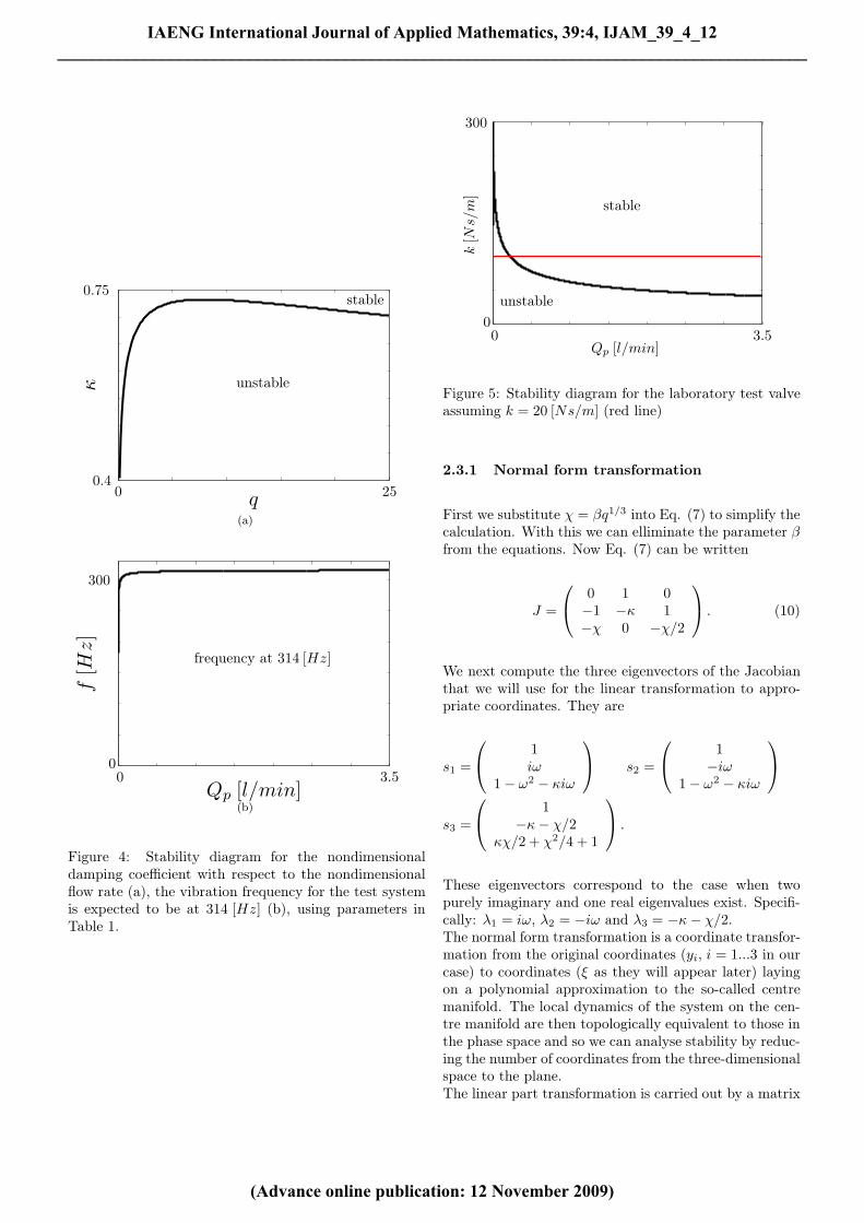
istic polinomial. With the transformation to dimensionalcoordinates we reach to the diagram shown in Figure 4(b)for the system’s vibration frequencies. Here we used pa-rameters that corresponds to the test equipment again(see Table 1). Figure 5. depicts the same stability dia-gram as 4(a) but in this case with physical parameters.We notice that the curve begins at the origin and has alocal extremum (maximum) at Qp = 0.05 [l/min]. If weassume, that our test valve can be characterized by a vis-cous damping coefficient of k = 20[Ns/m] (marked with ared line on Fig.5) then the unstable region obtained fromthe diagram is below Qp

∼= 0.25 [l/min]. Here again weshould mention that measuring the damping ratio is oneof the most difficult tasks when investigating dynamicalsystems experimentally.

2.3 Nonlinear analysis

Having found the presence of a Hopf bifurcation, we areinterested in the stability of the limit cycle. To do this,we will apply the normal form theory described for exam-ple in [4] and use the centre manifold reduction. We thencompute the first Lyapunov coefficient to determine sta-bility. We also compute the coefficient along the stabilitycurve obtained in Section 2.2 to see how it will changewhen varying some parameter. For simplicity we stick tothe case δ = 0.



q

κ

stable

unstable

0.75

0.40 25

(a)

Qp [l/min]

f[H

z]

frequency at 314 [Hz]

300

00 3.5

(b)

Figure 4: Stability diagram for the nondimensionaldamping coefficient with respect to the nondimensionalflow rate (a), the vibration frequency for the test systemis expected to be at 314 [Hz] (b), using parameters inTable 1.

300

00 3.5

Qp [l/min]

k[N

s/m

]

unstable

stable

Figure 5: Stability diagram for the laboratory test valveassuming k = 20 [Ns/m] (red line)

2.3.1 Normal form transformation

First we substitute χ = βq1/3 into Eq. (7) to simplify thecalculation. With this we can elliminate the parameter βfrom the equations. Now Eq. (7) can be written

J =

0 1 0−1 −κ 1−χ 0 −χ/2

. (10)

We next compute the three eigenvectors of the Jacobianthat we will use for the linear transformation to appro-priate coordinates. They are

s1 =

1iω

1 − ω2 − κiω

s2 =

1−iω

1 − ω2 − κiω

s3 =

1−κ − χ/2

κχ/2 + χ2/4 + 1

.

These eigenvectors correspond to the case when twopurely imaginary and one real eigenvalues exist. Specifi-cally: λ1 = iω, λ2 = −iω and λ3 = −κ − χ/2.The normal form transformation is a coordinate transfor-mation from the original coordinates (yi, i = 1...3 in ourcase) to coordinates (ξ as they will appear later) layingon a polynomial approximation to the so-called centremanifold. The local dynamics of the system on the cen-tre manifold are then topologically equivalent to those inthe phase space and so we can analyse stability by reduc-ing the number of coordinates from the three-dimensionalspace to the plane.The linear part transformation is carried out by a matrix



of the form

T =(

Re (s1) Im (s1) s3

)=

=

1 0 10 ω −κ − χ/2

1 − ω2 −κω κχ/2 + χ2/4 + 1

.

Here the columns of T represent the real and imaginaryparts of the first and the real third eigenvector. Our aimby choosing the elements of the transformation matrix isto obtain a system with real parameters after the trans-formation.

Before being able to do the transformation it is simplestto replace all nonlinear equations with their third orderTaylor expansion around the equilibrium to put the sys-tem into the following form

η′ = Jη + p3 (η) ,

where J is the linear coefficient matrix, e.g. the Jaco-bian of the system and p3 contains all the higher orderterms. Here we also consider small disturbances aroundthe equilibrium and put therefore η = y − y0 into theequations.The coordinate transformation is then following

η = Tξ, (11)

and the equation will have the form

Tξ′ = ATξ + p3 (Tξ) .

We can write such a system in first order form as

ξ′ = T−1AT︸︷︷︸

B

ξ + H (ξ) ,

or more conveniently in matrix form

ξ′1ξ′2ξ′3

=

0 ω 0−ω 0 00 0 −λ3

ξ1

ξ2

ξ3

+

H1 (ξ)H2 (ξ)H3 (ξ)

.

(12)Note that elements of the nonlinear vector H (ξ) maycontain any combination of products of the transformedcoordinates.

2.3.2 Centre manifold reduction

A problem arises when we wish to apply normal formtheory to our three-degrees-of-freedom system, since itis only applicable for systems of two degrees of freedom.Therefore we express the third coordinate ξ3 with theother two as a second-order Taylor series

ξ3 = h11ξ21 + h12ξ1ξ2 + h22ξ

22 + O

(ξ3

)(13)

We now need to find equations for the coefficients h11, h12

and h22. The idea we will use is to compute the derivative

of Eq. (13) and make it equal to the third equation ofour system in Eq. (12). Then we can express these coeffi-cients with those used for the third-order approximationof the nonlinear equation in the following way

2h11ξ1 ξ′1︸︷︷︸

ωξ2

+h12(xi′1ξ2 + ξ1 ξ′2︸︷︷︸

−ωξ1

) + 2h22ξ2ξ′2 =

= λ3

(h11ξ

21 + h12ξ1ξ2 + h22ξ

22

)+

+ H311ξ21 + H312ξ1ξ2 + H322ξ

22

︸︷︷︸

H3(ξ1,ξ2)

Here we can substitute ξ′1 and ξ′2 from the first two equa-tions of Eq. (12) as shown. This yields a linear system

for the unknown vector h = (h11 h12 h22)T

−λ3 −ω 02ω −λ3 −2ω0 ω −λ3

h11

h12

h22

=

H311

H312

H322

Now we know all the coefficients for the second order ex-pression of our third coordinate ξ3 that we can substituteinto the first two equations of Eq. (12) and collect all thecoefficients of the higher order terms. These we have tosubstitute into the so called Bautin formula [9] to obtainthe value for the first Lyapunov coefficient. The formulawe will use is as follows:

l(0) = 18

1ω [(a20 + a02) (−a11 + b20 − b02) +

(b20 + b02) (a20 − a02 + b11)]

+ 18 [3a30 + a12 + b21 + 3b03] ,

where aij and bij (i+j = 2, 3) are coefficients of the higherorder terms in the transformed equations. If l(0) < 0then the Hopf bifurcation is supercritical, e.g. a stablelimit cycle is born, and if l(0) > 0 then the bifurcation issubcritical and the limit cycle will be non-attracting.

2.3.3 Results

Figure 6 shows the Lyapunov coefficient along the stabil-ity curve obtained by the linear analysis. Note that thereis a change in the sign around κ = 0.67, below whichthe second Hopf bifurcation point will become subcriti-cal. Later we will present numerical continuation resultsshowing this to be the case.Now let we discuss further the values of the vibration fre-quency. As we obtained earlier in Section 2.2 there is ananalytical expression for the frequency

ω =√

a1 =

√

1 + χ−χ2 − 4 +

√

χ4 + 40χ2 + 16

8χ,

where χ = βq1/3.The limits of ω for large and small flow rates are

limχ→0

ω = 1 and limχ→∞

ω =√

3.



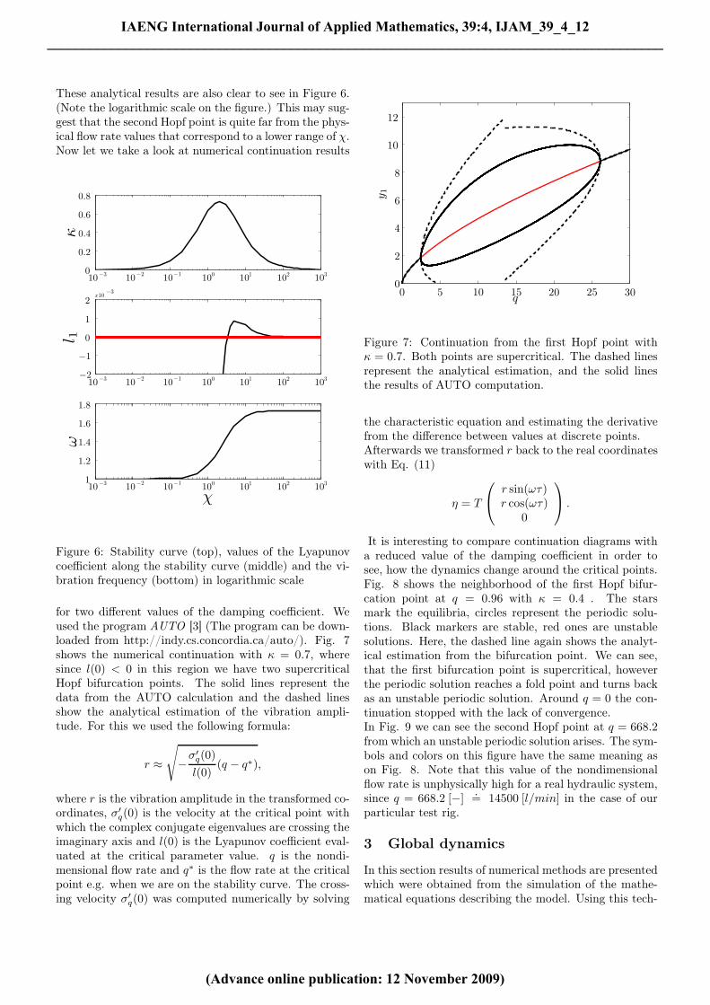
These analytical results are also clear to see in Figure 6.(Note the logarithmic scale on the figure.) This may sug-gest that the second Hopf point is quite far from the phys-ical flow rate values that correspond to a lower range of χ.Now let we take a look at numerical continuation results

χ

κl 1

ω

0

0

0

1

1

1

2

2

2

3

3

3

10101010101010

10101010101010

10101010101010

−1

−1

−1

−2

−2

−2

−3

−3

−3

1.2

1.4

1.6

1.8

0

0

0.2

0.4

0.6

0.8

−1

−2

1

1

2x10

−3

Figure 6: Stability curve (top), values of the Lyapunovcoefficient along the stability curve (middle) and the vi-bration frequency (bottom) in logarithmic scale

for two different values of the damping coefficient. Weused the program AUTO [3] (The program can be down-loaded from http://indy.cs.concordia.ca/auto/). Fig. 7shows the numerical continuation with κ = 0.7, wheresince l(0) < 0 in this region we have two supercriticalHopf bifurcation points. The solid lines represent thedata from the AUTO calculation and the dashed linesshow the analytical estimation of the vibration ampli-tude. For this we used the following formula:

r ≈

√

−σ′

q(0)

l(0)(q − q∗),

where r is the vibration amplitude in the transformed co-ordinates, σ′

q(0) is the velocity at the critical point withwhich the complex conjugate eigenvalues are crossing theimaginary axis and l(0) is the Lyapunov coefficient eval-uated at the critical parameter value. q is the nondi-mensional flow rate and q∗ is the flow rate at the criticalpoint e.g. when we are on the stability curve. The cross-ing velocity σ′

q(0) was computed numerically by solving

q

y 1

12

10

8

6

4

2

00 5 10 15 20 25 30

Figure 7: Continuation from the first Hopf point withκ = 0.7. Both points are supercritical. The dashed linesrepresent the analytical estimation, and the solid linesthe results of AUTO computation.

the characteristic equation and estimating the derivativefrom the difference between values at discrete points.Afterwards we transformed r back to the real coordinateswith Eq. (11)

η = T

r sin(ωτ)r cos(ωτ)

0

.

It is interesting to compare continuation diagrams witha reduced value of the damping coefficient in order tosee, how the dynamics change around the critical points.Fig. 8 shows the neighborhood of the first Hopf bifur-cation point at q = 0.96 with κ = 0.4 . The starsmark the equilibria, circles represent the periodic solu-tions. Black markers are stable, red ones are unstablesolutions. Here, the dashed line again shows the analyt-ical estimation from the bifurcation point. We can see,that the first bifurcation point is supercritical, howeverthe periodic solution reaches a fold point and turns backas an unstable periodic solution. Around q = 0 the con-tinuation stopped with the lack of convergence.In Fig. 9 we can see the second Hopf point at q = 668.2from which an unstable periodic solution arises. The sym-bols and colors on this figure have the same meaning ason Fig. 8. Note that this value of the nondimensionalflow rate is unphysically high for a real hydraulic system,since q = 668.2 [−]

.= 14500 [l/min] in the case of our

particular test rig.

3 Global dynamics

In this section results of numerical methods are presentedwhich were obtained from the simulation of the mathe-matical equations describing the model. Using this tech-



nique enables us to study the global dynamics of the sys-tem.

3.1 Numerical simulation

Numerical simulation is a simple and effective methodfor analysing dynamical systems and can be one step of adeeper investigation. It also enables us to treat systemswith discontinuity, e.g. when the solution trajectory or itsderivative is non continuous in the phase space. Of coursethere are several issues that we should take into consider-ation in order to obtain accurate results. For example thetype of ODE solver. There are numerous computer en-vironments that provide a numerical ODE solver such assome computer algebra packages or numerical mathemat-ical packages. We chose this latter environment since itprovides a wide range of solvers with adjustable error tol-erance and gives us a convenient way to manipulate dataand results using an effective programming language. Italso enables us to use the so called event handling featurethat is needed when treating impacting systems. We willuse this for the detection of crossings with the Poincarèsection as well.

In our simulation code we solve the nondimensional equa-tions. For this we use the physical parameters of the testrig mentioned earlier that was built up in the laboratory.Let us now present some results and in so doing explainsome of the particular features of our implementation.Fig. 10(a) shows impacting solutions. The red solutionline in the pressure plot is the equidistant qubic inter-polation of the solution that can be used for harmonicanalysis. An example spectrum of the pressure solutionof Fig. 10(a) is presented in Fig. 10(b). The pressure

q

y 1

3

00 0.2

Figure 8: Continuation from the first Hopf point with κ =0.4. The stable limit cycle is reaching a fold point, turnsback an become unstable. The dashed line represents theanalytical estimate.

q

y 1

0 10000

200

Figure 9: Continuation from the second Hopf point withκ = 0.4 showing the unstable limit cycle. The dashedline represents the analytical estimation.

time history is not sinusoidal, so we find higher frequencycomponents as well.

Now let us take a look at the phase space and see the sta-ble impacting limit cycle that exist for particular param-eters. This can be seen in Fig. 11. The nondimensionalparameters here are q = 3, κ = 1.25, β = 20 and δ = 10.Our program is capable of treating outer excitation inthe form of an explicit time-dependent flow rate distur-bance around a given value. This can be useful whencomparing numerical and experimental data. The rea-son of this feature comes from the experiments with thetest rig. We experienced that the influence of the peri-odic excitation of our gear pump unfortunately cannot beneglected. Furthermore, we extended our program withthe capability of producing so called brute force bifurca-tion diagrams that will be presented in the next section.These diagrams basically show how trajectory crossingswith a given Poincarè section changes when varying aparameter.

3.2 Numerical bifurcation diagrams

One of the earliest methods we can use during the inves-tigation of dynamical systems is to compute bifurcationdiagrams numerically. This can be performed by solv-ing the set of equations with an appropriate ODE solverin forward time. We should choose a suitable Poincarèmap in the phase space and let the solution trajectoriesbe recorded when crossing this surface. Starting multipleiterations with random initial conditions for each valueof the bifurcation parameter can lead us to the so called‘Monte Carlo’ diagram.

For all computation the following parameters were cho-



t [s]

t [s]

t [s]

x[m

m]

v[m

/s]

p[b

ar]

0.9

0.9

0.9

1.1

1.1

1.1

0

0

0

4

−1

30

(a)

x 1010

f [Hz]0 1000

0

3.5

(b)

Figure 10: A typical impacting solution of the system(a). Displacement (top), velocity (middle) and systempressure (bottom). The spectrum is depicted showingthe vibration frequency and its higher harmonical com-ponents (b).

sen unless otherwise stated: κ = 1.25, β = 20, δ = 10,r = 0.8. After an impact the velocity can be written asv+ = −rv−. Here v− is the velocity before and v+ after aparticular impact. The bifurcation parameter (the nondi-mensional flow rate) was varied between q = 0.01 − 10and for each q three random iterations were started froma 30×20×80 subset of phase space. Figure 12 shows thechosen Poincarè section in the phase space that is simplythe y2 = 0 plane.Now we should take a closer look at the results of thecomputation that can be seen in Figure 13. There aresome interesting regions in the figure that should be dis-cussed. Let us consider reducing q from a high value to-wards zero. At about q = 9.18 a stable limit cycle is bornand it grows quick in amplitude with further decrease ofthe bifurcation parameter. This extreme growth can beexplained from the fact that the first Lyapunov coefficientremains relative close to zero but is clearly negative for

y1y2

y 3

0

25

−5

5

0

3

Figure 11: Impacting limit cycle for a nondimensionalflow rate of q = 3. The constant parameters are κ = 1.25,β = 20 and δ = 10.

Figure 12: Solution trajectories impacting at the y1 =0 plane. The yellow plane depicts the chosen Poincarèsection, the y2 = 0 plane.

values of q lower than about q ∼= 17338 as we obtained insubsection 2.3. A typical solution trajectory within thisregion is depicted in Figure 14(a).At q ∼= 7.54 a grazing bifurcation occurs. This meansthat the amplitude of the vibration grows and reachesthe impacting barrier y1 = 0 which means that the dis-placement x of the valve poppet has reached 0, the valueat the valve seat in our physical system. At grazing, onlyzero velocity impacts occur, this also means that the re-set map that is used for determining the velocity afterimpact is the identity map itself, the velocity before andafter the impact are both equal to zero.With further decrease of the dimensionless flow rate,period-three and period-two impacting solutions can beseen between q = 6.1− 7.54. Parts of this region seem to



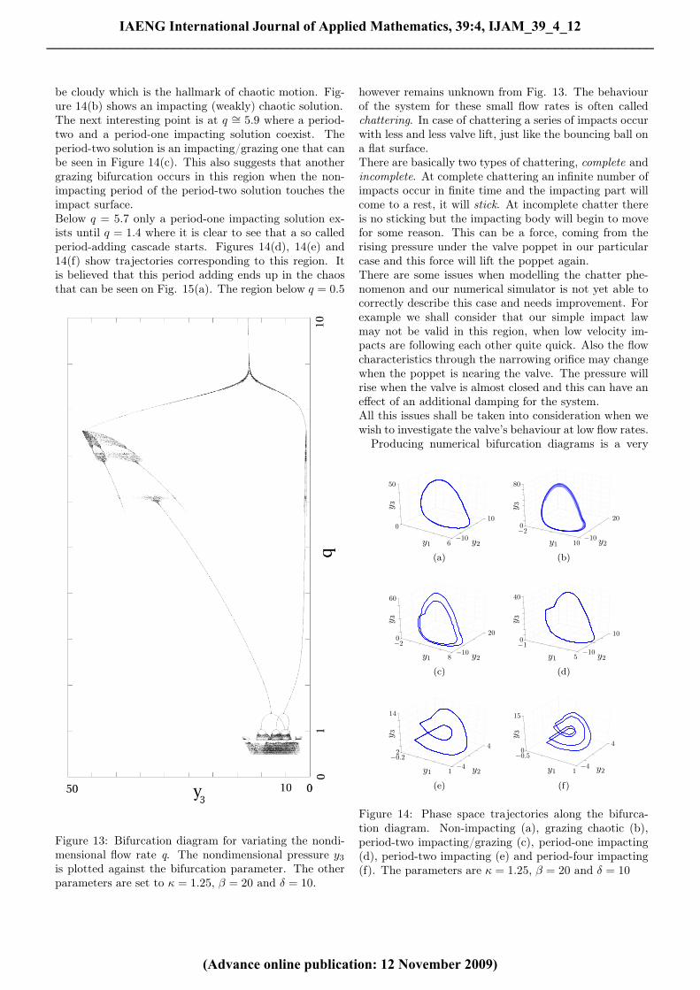
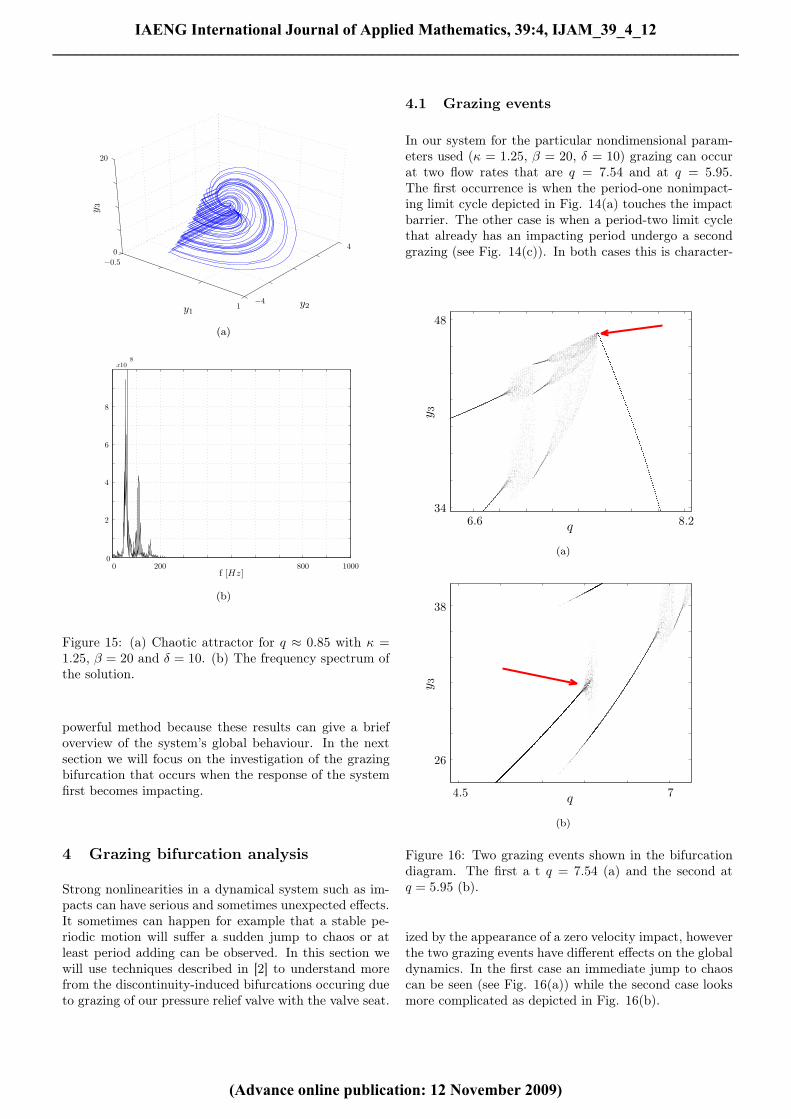
be cloudy which is the hallmark of chaotic motion. Fig-ure 14(b) shows an impacting (weakly) chaotic solution.The next interesting point is at q ∼= 5.9 where a period-two and a period-one impacting solution coexist. Theperiod-two solution is an impacting/grazing one that canbe seen in Figure 14(c). This also suggests that anothergrazing bifurcation occurs in this region when the non-impacting period of the period-two solution touches theimpact surface.Below q = 5.7 only a period-one impacting solution ex-ists until q = 1.4 where it is clear to see that a so calledperiod-adding cascade starts. Figures 14(d), 14(e) and14(f) show trajectories corresponding to this region. Itis believed that this period adding ends up in the chaosthat can be seen on Fig. 15(a). The region below q = 0.5

Figure 13: Bifurcation diagram for variating the nondi-mensional flow rate q. The nondimensional pressure y3

is plotted against the bifurcation parameter. The otherparameters are set to κ = 1.25, β = 20 and δ = 10.

however remains unknown from Fig. 13. The behaviourof the system for these small flow rates is often calledchattering. In case of chattering a series of impacts occurwith less and less valve lift, just like the bouncing ball ona flat surface.There are basically two types of chattering, complete andincomplete. At complete chattering an infinite number ofimpacts occur in finite time and the impacting part willcome to a rest, it will stick. At incomplete chatter thereis no sticking but the impacting body will begin to movefor some reason. This can be a force, coming from therising pressure under the valve poppet in our particularcase and this force will lift the poppet again.There are some issues when modelling the chatter phe-nomenon and our numerical simulator is not yet able tocorrectly describe this case and needs improvement. Forexample we shall consider that our simple impact lawmay not be valid in this region, when low velocity im-pacts are following each other quite quick. Also the flowcharacteristics through the narrowing orifice may changewhen the poppet is nearing the valve. The pressure willrise when the valve is almost closed and this can have aneffect of an additional damping for the system.All this issues shall be taken into consideration when wewish to investigate the valve’s behaviour at low flow rates.

Producing numerical bifurcation diagrams is a very

y1 y2

y 3

0

50

−10

10

6

(a)

y1 y2

y 30

80

−10

20

−2

10

(b)

y1 y2

y 3

0

60

−10

20

−2

8

(c)

y1 y2

y 3

0

40

−10

10

−1

5

(d)

y1 y2

y 3

2

14

−4

4

−0.2

1

(e)

y1 y2

y 3

0

15

−4

4

−0.5

1

(f)

Figure 14: Phase space trajectories along the bifurca-tion diagram. Non-impacting (a), grazing chaotic (b),period-two impacting/grazing (c), period-one impacting(d), period-two impacting (e) and period-four impacting(f). The parameters are κ = 1.25, β = 20 and δ = 10



y1y2

y 3

0

20

−4

4

−0.5

1

(a)

f [Hz]0 200 800 1000

x108

0

2

4

6

8

(b)

Figure 15: (a) Chaotic attractor for q ≈ 0.85 with κ =1.25, β = 20 and δ = 10. (b) The frequency spectrum ofthe solution.

powerful method because these results can give a briefoverview of the system’s global behaviour. In the nextsection we will focus on the investigation of the grazingbifurcation that occurs when the response of the systemfirst becomes impacting.

4 Grazing bifurcation analysis

Strong nonlinearities in a dynamical system such as im-pacts can have serious and sometimes unexpected effects.It sometimes can happen for example that a stable pe-riodic motion will suffer a sudden jump to chaos or atleast period adding can be observed. In this section wewill use techniques described in [2] to understand morefrom the discontinuity-induced bifurcations occuring dueto grazing of our pressure relief valve with the valve seat.

4.1 Grazing events

In our system for the particular nondimensional param-eters used (κ = 1.25, β = 20, δ = 10) grazing can occurat two flow rates that are q = 7.54 and at q = 5.95.The first occurrence is when the period-one nonimpact-ing limit cycle depicted in Fig. 14(a) touches the impactbarrier. The other case is when a period-two limit cyclethat already has an impacting period undergo a secondgrazing (see Fig. 14(c)). In both cases this is character-

q

y 3

6.6 8.234

48

(a)

q

y 3

4.5 7

26

38

(b)

Figure 16: Two grazing events shown in the bifurcationdiagram. The first a t q = 7.54 (a) and the second atq = 5.95 (b).

ized by the appearance of a zero velocity impact, howeverthe two grazing events have different effects on the globaldynamics. In the first case an immediate jump to chaoscan be seen (see Fig. 16(a)) while the second case looksmore complicated as depicted in Fig. 16(b).



4.2 Bifurcation scenario at grazing

We carried out an analytical investigation for the firstcase (where q = 7.54) to find out what type of grazingbifurcation we have to deal with. For this we used thetheory for nonsmooth systems described in [2]. First wehave to find the grazing limit cycle exactly. Our bifurca-tion diagram in Fig.13 is very helpful, because it containsthe critical flow rate q and the nondimensional pressurey3 can also be obtained. Since we chose the zero velocityplane as our Poincarè section y2 = 0 and at grazing ourdisplacement is also zero. We now have initial conditionsthat correspond to the last non-impacting limit cycle.The next step is to solve the so called linear variationalequations along the limit cycle, to obtain the monodromymatrix. These equations can be written in following form:

w = Jw, (14)

where J is the linear part of the nonlinear system definedin Eq. (5) but without substituting the equilibrium. So(14) can be written in the form:

w1

w2

w3

=

0 1 0−1 −κ 1

−β√

y3 0 − 12

βy1√y3

w1

w2

w3

,

and J is linear with respect to w. We have to solve(14) together with the system’s equations for the periodT of the grazing limit cycle three times with the initialconditions

(w01

1 , w012 , w01

3

)= (1, 0, 0),

(w02

1 , w022 , w02

3

)=

(0, 1, 0) and(w03

1 , w032 , w03

3

)= (0, 0, 1). We can then com-

pose the monodromy matrix M from the solution w (T )after one complete period in following way:

M =(w01 (T )w02 (T )w03 (T )

)

We now have to compute the eigenvalues of M and applythe theory described in [2].For the grazing flow rate q = 7.54 we can find(y01 , y

02 , y

03

)(0, 0, 47.07) as initial condition of the graz-

ing limit cycle. When we integrate for one period (T =2.6547 for this flow rate) and solve the linear variationalequations we obtain that

M =

0.5972 0.0450 −0.011113.4466 1.5311 −0.130640.8328 5.1828 −0.2744

,

whose eigenvalues are ν1 = 1, ν2 = 0.8537 and ν3 = 0. Itis necessary to have one eigenvalue that is equal to 1. ν3

does not necessarily have to be zero, but presumably itis close to and the difference may be beyond the compu-tation tolerance.The second eigenvalue gives us important informationabout the scenario after the grazing event. First of allit has to be less than 1 because the grazing limit cycle isattracting, e.g. it is stable.According to theory there are three scenarios:

1. If 0 < ν < 1/4 then grazing is followed by a periodadding, in which the periodic bands overlap,

2. if 1/4 < ν < 2/3 then chaotic and stable periodicsolutions are alternating and periodic motion formsa period adding cascade,

3. if 2/3 < ν < 1 then there is a sudden jump to chaosto obtain, and the chaotic attractor’s size is squareroot proportional to the bifurcation parameter.

Since we have 2/3 < ν2 < 1, a robust chaotic attractorarises, as it can also be seen in Fig. 16(a). It is also easyto notice that it is growing like a square root function.According to literature [2] this behaviour is characteristicto impacting systems. Note that this approach is onlyvalid if we assume that the discontinuity map has quasione-dimensional behaviour. The literature [2] containslots of examples and presents various bifurcation dia-grams, also ones that refer to the other two scenarios. Anexample figure for the first case, e.g. when 0 < ν < 1/4looks very similar to our second grazing scenario thatarises at q = 5.95. This could be analysed with the sametechnique in a latter investigation.

4.3 The three-dimensional square root map

Impacting systems have a so called square root-type non-linearity. This means that the bifurcation scenario thatoccur at grazing can be described by a square root map.Such a map can be written in general form

x 7→ Mx + Nµ + Ey ,if H (x, µ) < 0, (15)

andx 7→ Mx + Nµ ,if H (x, µ) > 0.

M is the monodromy matrix mentioned earlier, N is acolumn vector that is obtained by the same linear vari-ational equations as the matrix M but we have to addthe partial derivative with respect to the bifurcation pa-rameter. In our case this only means the addition of β to

the third equation since∂y′

3

∂q = β. At this time we haveto solve the equations around the grazing periodic orbitwith the initial conditions (0, 0, 0). In our particular casewe obtain

N = (0.2269− 0.1939− 7.3400)T

.

The term Ey in Eq.(15) contains the square root singu-larity in general and H (x, µ) in our case is the minimumdisplacement of the trajectory if we would not allow anyimpact at all. There are basically two types of discon-tinuity maps that are used when investigating grazingbifurcations, the Poincarè-section discontinuity mappingand the Zero time discontinuity mapping. In our investi-gation we will only focus on the zero time discontinuitymap, e.g. ZDM. It can be composed by taking an initial



H (x, µ)

v

x1

x2 x3

x4

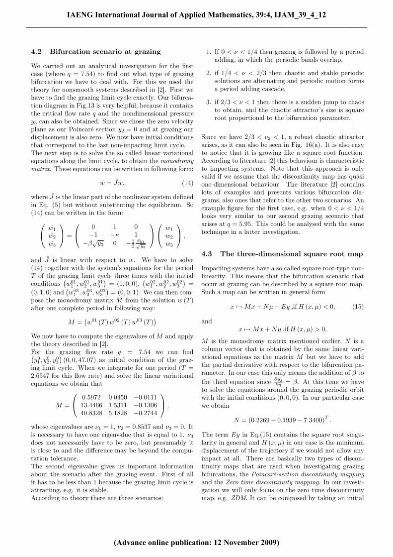
Figure 17: The ZDM maps in practice. The point x1 ismapped to the point x4 in which the solution is integratedbackward time from x3 for the time that elapsed betweenthe points x1 and x2.

point arbitrary close to the grazing point and integratingit forward in time until we stop at the impact surface andmeasure the elapsed time. Then we apply the impact lawbut this time we integrate backward in time for the sametime period that was recorded. See Fig.17 that shows animpacting trajectory together with the important points.For our investigation we will use following analytical ap-proach of the ZDM that can be found in [2]

x 7→ Mx + Nµ ,if H (x, µ) > 0 and

x 7→ Mx +√

2a∗W (x)y + Nµ ,if H (x, µ) < 0 ,

where a∗ is the acceleration at the graing point, W (x)contains the coefficient of restitution, µ = q − qcrit isthe bifurcation parameter and y =

√−x represents the

square root singularity. In our particular case we cansubstitute

a∗ = p∗ − δ and

W (x) =

01 + r

0

,

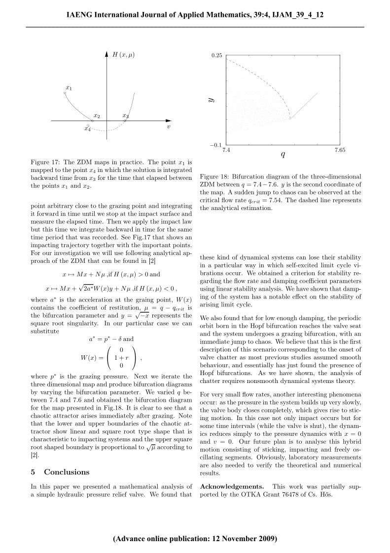
where p∗ is the grazing pressure. Next we iterate thethree dimensional map and produce bifurcation diagramsby varying the bifurcation parameter. We varied q be-tween 7.4 and 7.6 and obtained the bifurcation diagramfor the map presented in Fig.18. It is clear to see that achaotic attractor arises immediately after grazing. Notethat the lower and upper boundaries of the chaotic at-tractor show linear and square root type shape that ischaracteristic to impacting systems and the upper squareroot shaped boundary is proportional to

√µ according to

[2].

5 Conclusions

In this paper we presented a mathematical analysis ofa simple hydraulic pressure relief valve. We found that

q

y

7.4 7.65−0.1

0.25

Figure 18: Bifurcation diagram of the three-dimensionalZDM between q = 7.4−7.6. y is the second coordinate ofthe map. A sudden jump to chaos can be observed at thecritical flow rate qcrit = 7.54. The dashed line representsthe analytical estimation.

these kind of dynamical systems can lose their stabilityin a particular way in which self-excited limit cycle vi-brations occur. We obtained a criterion for stability re-garding the flow rate and damping coefficient parametersusing linear stability analysis. We have shown that damp-ing of the system has a notable effect on the stability ofarising limit cycle.

We also found that for low enough damping, the periodicorbit born in the Hopf bifurcation reaches the valve seatand the system undergoes a grazing bifurcation, with animmediate jump to chaos. We believe that this is the firstdescription of this scenario corresponding to the onset ofvalve chatter as most previous studies assumed smoothbehaviour, and essentially has just found the presence ofHopf bifurcations. As we have shown, the analysis ofchatter requires nonsmooth dynamical systems theory.

For very small flow rates, another interesting phenomenaoccur: as the pressure in the system builds up very slowly,the valve body closes completely, which gives rise to stic-ing motion. In this case not only impact occurs but forsome time intervals (while the valve is shut), the dynam-ics reduces simply to the pressure dynamics with x = 0and v = 0. Our future plan is to analyse this hybridmotion consisting of sticking, impacting and freely os-cillating segments. Obviously, laboratory measurementsare also needed to verify the theoretical and numericalresults.

Acknowledgements. This work was partially sup-ported by the OTKA Grant 76478 of Cs. Hős.



References

[1] W. Bolton. Pneumatic and hydraulic systems.Butterworth-Heinemann, 1997.

[2] M. di Bernardo, C. J. Budd, A. R. Champneys, andP. Kowalczyk. Piecewise-smooth dynamical systems.Springer, 2007.

[3] E. J. Doedel, R. C. Paffenroth, A. R. Champneys,T. R. Fairgrieve, Y. A. Kuznetsov, B. E. Oldeman,B. Sanstede, and X. Wang. AUTO 2000 : Continu-ation and Bifurcation Software for Ordinary Differ-ential Equations, 2006.

[4] J. Guckenheimer and P. Holmes. Nonlinear oscilla-tions, dynamical systems, and bifurcations of vectorfields. Springer, 1983.

[5] S. Hayashi. Instability of poppet valve circuit. JSMEInternational Journal, 38(3), 1995.

[6] S. Hayashi, T. Hayase, and T. Kurahashi. Chaosin a hydraulic control valve. Journal of fluids andstructures, (11):693–716, 1997.

[7] K. Kasai. On the stability of a poppet valve with anelastic support. Bulletin of JSME, 11(48), 1968.

[8] F. X. Kay. Pneumatics for industry. The MachineryPublishing Co. Ltd., 1959.

[9] Yuri A. Kuznetsov. Elements of applied bifurcationtheory. Springer, 1997.

[10] H. L. Stewart. Hydraulic and pneumatic power forproduction. The Industrial Press, 1963.

[11] H. Thomann. Oscillations of a simple valve con-nected to a pipe. Journal of Applied Mathematicsand Physics, 1976.



Nonlinear Analysis of a Single Stage Pressure Relief Valve · 2009-11-10 · Nonlinear Analysis of...

Documents

Transcript of Nonlinear Analysis of a Single Stage Pressure Relief Valve · 2009-11-10 · Nonlinear Analysis of...