Nonhomogeneous Linear Systems of Differential...
57
Nonhomogeneous Linear Systems of Differential Equations: the method of variation of parameters Xu-Yan Chen
Transcript of Nonhomogeneous Linear Systems of Differential...

Nonhomogeneous Linear Systems of
Differential Equations:
the method of variation of parameters
Xu-Yan Chen

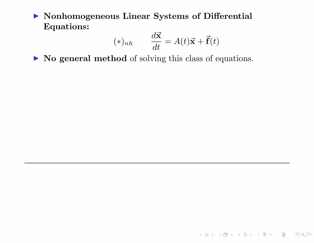
◮ Nonhomogeneous Linear Systems of DifferentialEquations:
(∗)nh
d~x
dt= A(t)~x +~f(t)
◮ Nonhomogeneous Linear Systems of DifferentialEquations:
(∗)nh
d~x
dt= A(t)~x +~f(t)
◮ No general method of solving this class of equations.

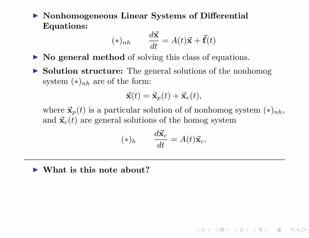
◮ Nonhomogeneous Linear Systems of DifferentialEquations:
(∗)nh
d~x
dt= A(t)~x +~f(t)
◮ No general method of solving this class of equations.
◮ Solution structure: The general solutions of the nonhomogsystem (∗)nh are of the form:
~x(t) = ~xp(t) + ~xc(t),
where ~xp(t) is a particular solution of of nonhomog system (∗)nh,and ~xc(t) are general solutions of the homog system
(∗)h
d~xc
dt= A(t)~xc.
◮ What is this note about?

◮ Nonhomogeneous Linear Systems of DifferentialEquations:
(∗)nh
d~x
dt= A(t)~x +~f(t)
◮ No general method of solving this class of equations.
◮ Solution structure: The general solutions of the nonhomogsystem (∗)nh are of the form:
~x(t) = ~xp(t) + ~xc(t),
where ~xp(t) is a particular solution of of nonhomog system (∗)nh,and ~xc(t) are general solutions of the homog system
(∗)h
d~xc
dt= A(t)~xc.
◮ What is this note about?Variation of Parameters.
If the solutions ~xc(t) ofthe homogeneous system(∗)h have been providedor prepared,
⇒we can solve the nonhomogsystem (∗)nh.
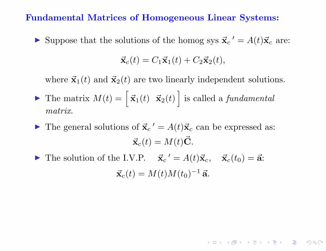
Fundamental Matrices of Homogeneous Linear Systems:

Fundamental Matrices of Homogeneous Linear Systems:
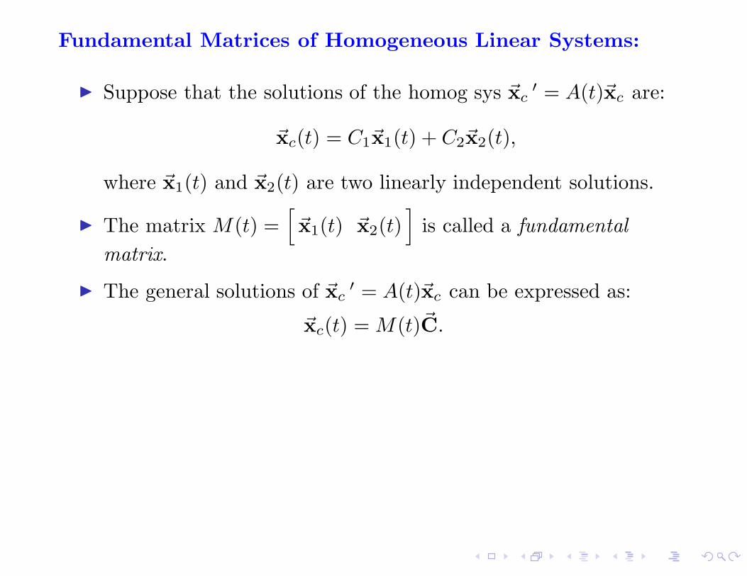
◮ Suppose that the solutions of the homog sys ~xc′ = A(t)~xc are:
~xc(t) = C1~x1(t) + C2~x2(t),
where ~x1(t) and ~x2(t) are two linearly independent solutions.

Fundamental Matrices of Homogeneous Linear Systems:
◮ Suppose that the solutions of the homog sys ~xc′ = A(t)~xc are:
~xc(t) = C1~x1(t) + C2~x2(t),
where ~x1(t) and ~x2(t) are two linearly independent solutions.
◮ The matrix M(t) =[
~x1(t) ~x2(t)]
is called a fundamental
matrix.

Fundamental Matrices of Homogeneous Linear Systems:
◮ Suppose that the solutions of the homog sys ~xc′ = A(t)~xc are:
~xc(t) = C1~x1(t) + C2~x2(t),
where ~x1(t) and ~x2(t) are two linearly independent solutions.
◮ The matrix M(t) =[
~x1(t) ~x2(t)]
is called a fundamental
matrix.
◮ The general solutions of ~xc′ = A(t)~xc can be expressed as:
~xc(t) = M(t)~C.
Since
~xc(t) = C1~x1(t) + C2~x2(t) =
[
~x1(t) ~x2(t)
] [
C1
C2
]
= M(t)~C
Fundamental Matrices of Homogeneous Linear Systems:
◮ Suppose that the solutions of the homog sys ~xc′ = A(t)~xc are:
~xc(t) = C1~x1(t) + C2~x2(t),
where ~x1(t) and ~x2(t) are two linearly independent solutions.
◮ The matrix M(t) =[
~x1(t) ~x2(t)]
is called a fundamental
matrix.
◮ The general solutions of ~xc′ = A(t)~xc can be expressed as:
~xc(t) = M(t)~C.
◮ The solution of the I.V.P. ~xc′ = A(t)~xc, ~xc(t0) = ~a:
~xc(t) = M(t)M(t0)−1 ~a.
Since
~xc(t0) = M(t0)~C = ~a ⇒ ~C = M(t0)−1 ~a
⇒ ~xc(t) = M(t)M(t0)−1 ~a.
Fundamental Matrices of Homogeneous Linear Systems:
◮ Suppose that the solutions of the homog sys ~xc′ = A(t)~xc are:
~xc(t) = C1~x1(t) + C2~x2(t),
where ~x1(t) and ~x2(t) are two linearly independent solutions.
◮ The matrix M(t) =[
~x1(t) ~x2(t)]
is called a fundamental
matrix.
◮ The general solutions of ~xc′ = A(t)~xc can be expressed as:
~xc(t) = M(t)~C.
◮ The solution of the I.V.P. ~xc′ = A(t)~xc, ~xc(t0) = ~a:
~xc(t) = M(t)M(t0)−1 ~a.
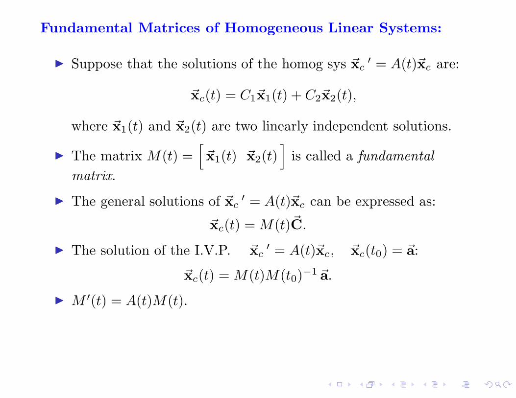
◮ M ′(t) = A(t)M(t).
◮ M(t) is an invertible matrix for any t.
◮ The fundamental matrices are not unique.

Nonhomogeneous Linear Systems of Differential Equations:
(∗)nh ~x′ = A(t)~x +~f(t).
The Method of Variation of Parameters:

Nonhomogeneous Linear Systems of Differential Equations:
(∗)nh ~x′ = A(t)~x +~f(t).
The Method of Variation of Parameters:
◮ Suppose that the homogeneous system ~x′c = A(t)~xc is solved,
with
{
a fundamental matrix M(t),
the complementary solutions ~xc(t) = M(t)~C.

Nonhomogeneous Linear Systems of Differential Equations:
(∗)nh ~x′ = A(t)~x +~f(t).
The Method of Variation of Parameters:
◮ Suppose that the homogeneous system ~x′c = A(t)~xc is solved,
with
{
a fundamental matrix M(t),
the complementary solutions ~xc(t) = M(t)~C.
◮ Set ~x(t) = M(t)~u(t).
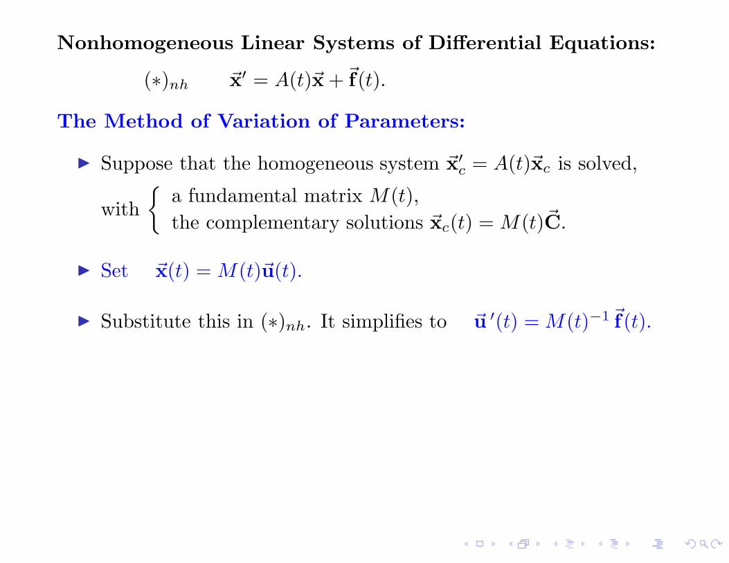
Nonhomogeneous Linear Systems of Differential Equations:
(∗)nh ~x′ = A(t)~x +~f(t).
The Method of Variation of Parameters:
◮ Suppose that the homogeneous system ~x′c = A(t)~xc is solved,
with
{
a fundamental matrix M(t),
the complementary solutions ~xc(t) = M(t)~C.
◮ Set ~x(t) = M(t)~u(t).
◮ Substitute this in (∗)nh. It simplifies to ~u ′(t) = M(t)−1~f (t).
Proof:`
M(t)~u(t)´′
= A(t)M(t)~u(t) +~f(t)
⇒ M ′(t)~u(t) + M(t)~u ′(t) = A(t)M(t)~u(t) +~f(t).
Since M ′(t) = A(t)M(t), we obtain M(t)~u ′(t) = ~f(t).
Take the inverse: ~u ′(t) = M(t)−1 ~f(t).
◮ Integrate to get ~u(t).
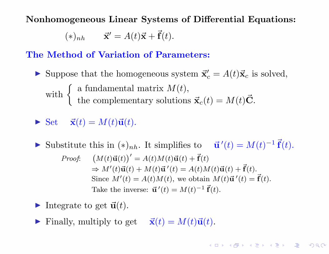
◮ Finally, multiply to get ~x(t) = M(t)~u(t).

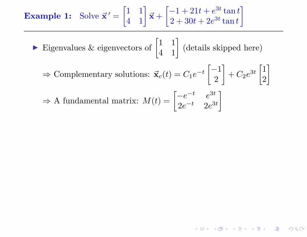
Example 1: Solve ~x ′ =
[
1 14 1
]
~x +
[
−1 + 21t + e3t tan t
2 + 30t + 2e3t tan t
]
Example 1: Solve ~x ′ =
[
1 14 1
]
~x +
[
−1 + 21t + e3t tan t
2 + 30t + 2e3t tan t
]
◮ Eigenvalues & eigenvectors of
[
1 14 1
]
(details skipped here)
⇒ Complementary solutions: ~xc(t) = C1e−t
[
−12
]
+ C2e3t
[
12
]
⇒ A fundamental matrix: M(t) =
[
−e−t e3t
2e−t 2e3t
]

Example 1: Solve ~x ′ =
[
1 14 1
]
~x +
[
−1 + 21t + e3t tan t
2 + 30t + 2e3t tan t
]
◮ Eigenvalues & eigenvectors of
[
1 14 1
]
(details skipped here)
⇒ Complementary solutions: ~xc(t) = C1e−t
[
−12
]
+ C2e3t
[
12
]
⇒ A fundamental matrix: M(t) =
[
−e−t e3t
2e−t 2e3t
]
◮ Set ~x(t) = M(t)~u(t)
Example 1: Solve ~x ′ =
[
1 14 1
]
~x +
[
−1 + 21t + e3t tan t
2 + 30t + 2e3t tan t
]
◮ Eigenvalues & eigenvectors of
[
1 14 1
]
(details skipped here)
⇒ Complementary solutions: ~xc(t) = C1e−t
[
−12
]
+ C2e3t
[
12
]
⇒ A fundamental matrix: M(t) =
[
−e−t e3t
2e−t 2e3t
]
◮ Set ~x(t) = M(t)~u(t)
◮ The original system is simplified to ~u ′(t) = M(t)−1~f(t):
~u ′(t) =
[
−e−t e3t
2e−t 2e3t
]−1 [
−1 + 21t + e3t tan t
2 + 30t + 2e3t tan t
]
=1
−4e2t
[
2e3t −e3t
−2e−t −e−t
] [
−1 + 21t + e3t tan t
2 + 30t + 2e3t tan t
]
=
[
(1 − 3t)et
18te−3t + tan t
]
.

Example 1 (continued): ~x ′ =
[
1 14 1
]
~x +
[
−1 + 21t + e3t tan t
2 + 30t + 2e3t tan t
]
◮ Integrate ~u ′(t) =
[
(1 − 3t)et
18te−3t + tan t
]
:
R
(1 − 3t)etdt = (1 − 3t)et −R
(−3)etdt = (1 − 3t)et + 3et + C,R
18te−3tdt = −6te−3t −R
(−6)e−3tdt = −6te−3t − 2e−3t + C,R
tan t dt = − ln | cos t| + C.
⇒ ~u(t) =
[
(4 − 3t)et + C1
(−2 − 6t)e−3t − ln | cos t| + C2
]
.
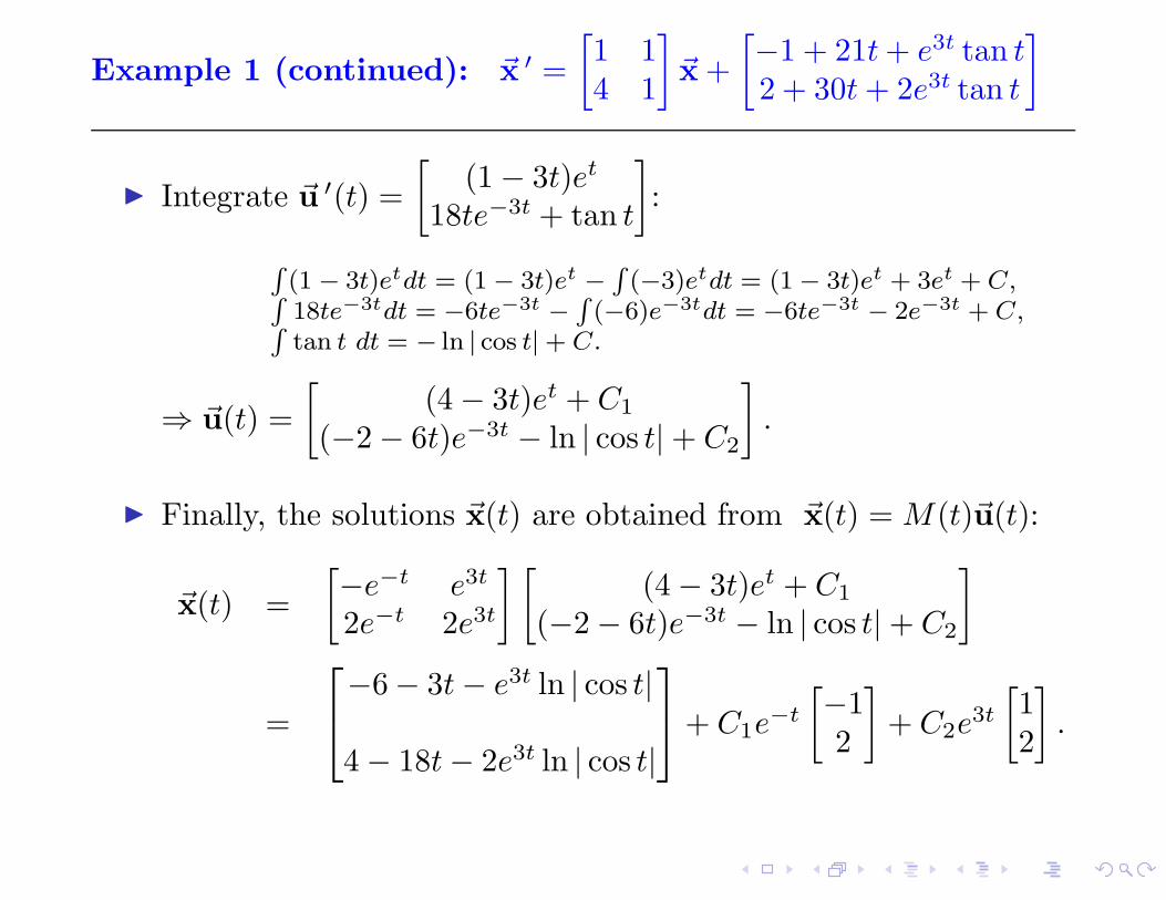
Example 1 (continued): ~x ′ =
[
1 14 1
]
~x +
[
−1 + 21t + e3t tan t
2 + 30t + 2e3t tan t
]
◮ Integrate ~u ′(t) =
[
(1 − 3t)et
18te−3t + tan t
]
:
R
(1 − 3t)etdt = (1 − 3t)et −R
(−3)etdt = (1 − 3t)et + 3et + C,R
18te−3tdt = −6te−3t −R
(−6)e−3tdt = −6te−3t − 2e−3t + C,R
tan t dt = − ln | cos t| + C.
⇒ ~u(t) =
[
(4 − 3t)et + C1
(−2 − 6t)e−3t − ln | cos t| + C2
]
.
◮ Finally, the solutions ~x(t) are obtained from ~x(t) = M(t)~u(t):
~x(t) =
[
−e−t e3t
2e−t 2e3t
] [
(4 − 3t)et + C1
(−2 − 6t)e−3t − ln | cos t| + C2
]
=
−6 − 3t − e3t ln | cos t|
4 − 18t − 2e3t ln | cos t|
+ C1e−t
[
−12
]
+ C2e3t
[
12
]
.

Example 2: Solve 2y′′ − y′ − y =3e
3
2t
1 + et.

Example 2: Solve 2y′′ − y′ − y =3e
3
2t
1 + et.
◮ Set ~x =
[
x1
x2
]
=
[
y
y′
]
:
2y′′ − y′ − y = 3e3
2t
1+et ⇔ ~x ′ =
[
0 112
12
]
~x +
[
03e
3
2t
2(1+et)
]

Example 2: Solve 2y′′ − y′ − y =3e
3
2t
1 + et.
◮ Set ~x =
[
x1
x2
]
=
[
y
y′
]
:
2y′′ − y′ − y = 3e3
2t
1+et ⇔ ~x ′ =
[
0 112
12
]
~x +
[
03e
3
2t
2(1+et)
]
◮ Characteristic roots ⇒ yc(t) = C1e− 1
2t + C2e
t

Example 2: Solve 2y′′ − y′ − y =3e
3
2t
1 + et.
◮ Set ~x =
[
x1
x2
]
=
[
y
y′
]
:
2y′′ − y′ − y = 3e3
2t
1+et ⇔ ~x ′ =
[
0 112
12
]
~x +
[
03e
3
2t
2(1+et)
]
◮ Characteristic roots ⇒ yc(t) = C1e− 1
2t + C2e
t
◮ yc(t) ⇒ complem. solutions of the system & a fund. matrix:
~xc(t) = C1
[
e−1
2t
− 12e−
1
2t
]
+ C2
[
et
et
]
, M(t) =
[
e−1
2t et
− 12e−
1
2t et
]
.
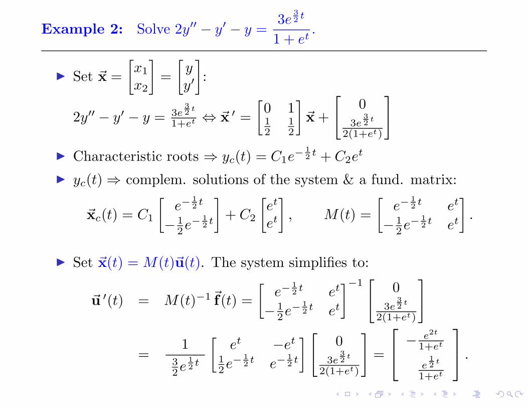
Example 2: Solve 2y′′ − y′ − y =3e
3
2t
1 + et.
◮ Set ~x =
[
x1
x2
]
=
[
y
y′
]
:
2y′′ − y′ − y = 3e3
2t
1+et ⇔ ~x ′ =
[
0 112
12
]
~x +
[
03e
3
2t
2(1+et)
]
◮ Characteristic roots ⇒ yc(t) = C1e− 1
2t + C2e
t
◮ yc(t) ⇒ complem. solutions of the system & a fund. matrix:
~xc(t) = C1
[
e−1
2t
− 12e−
1
2t
]
+ C2
[
et
et
]
, M(t) =
[
e−1
2t et
− 12e−
1
2t et
]
.
◮ Set ~x(t) = M(t)~u(t). The system simplifies to:
~u ′(t) = M(t)−1~f(t) =
[
e−1
2t et
− 12e−
1
2t et
]−1[
03e
3
2t
2(1+et)
]
=1
32e
1
2t
[
et −et
12e−
1
2t e−
1
2t
]
[
03e
3
2t
2(1+et)
]
=
− e2t
1+et
e1
2t
1+et
.

Example 2 (continued): 2y′′ − y′ − y = 3e3
2t
1+et
◮ Integrate ~u ′(t) =
− e2t
1+et
e1
2t
1+et
:
R
e2t
1+et dt =R
s1+s
ds =R
(1 − 1
1+s)ds = s − ln |1 + s| + C
(substituted s = et),R
e1
2t
1+etdt =
R
2
1+s2ds = 2arctan s + C (substituted s = et/2).
⇒ ~u(t) =
[
−et + ln(1 + et) + C1
2 arctan(e1
2t) + C2
]
.
◮ Finally, the solutions ~x(t) are obtained from ~x(t) = M(t)~u(t):
~x(t) =
[
e−1
2t et
− 12e−
1
2t et
] [
−et + ln(1 + et) + C1
2 arctan(e1
2t) + C2
]
= · · · ,
y(t) = x1(t)
= −e1
2t + e−
1
2t ln(1 + et) + 2et arctan(e
1
2t) + C1e
− 1
2t + C2e
t.
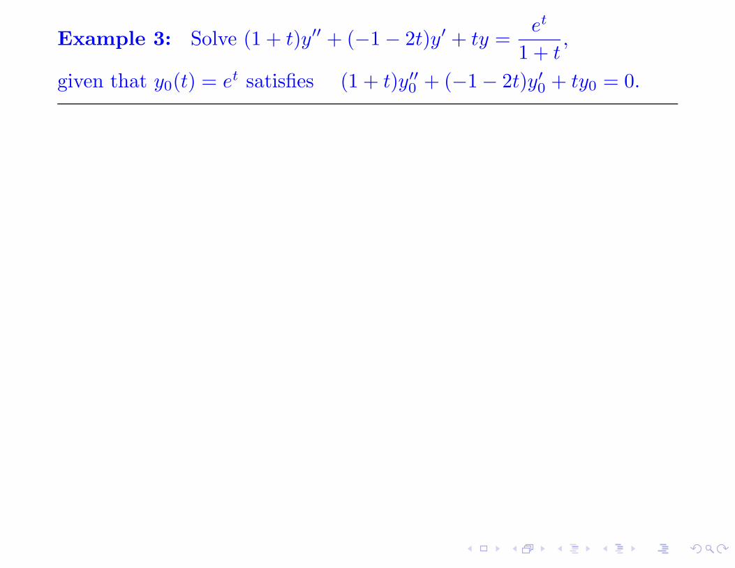
Example 3: Solve (1 + t)y′′ + (−1 − 2t)y′ + ty =et
1 + t,
given that y0(t) = et satisfies (1 + t)y′′0 + (−1 − 2t)y′
0 + ty0 = 0.

Example 3: Solve (1 + t)y′′ + (−1 − 2t)y′ + ty =et
1 + t,
given that y0(t) = et satisfies (1 + t)y′′0 + (−1 − 2t)y′
0 + ty0 = 0.
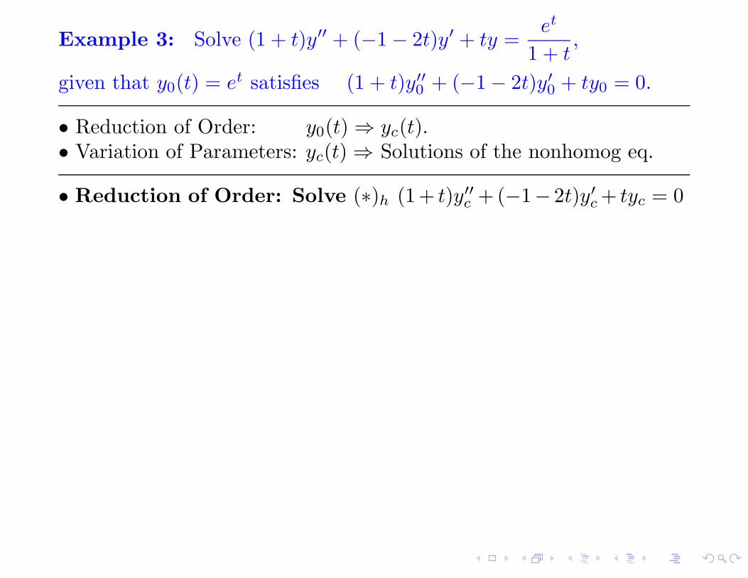
• Reduction of Order: y0(t) ⇒ yc(t).• Variation of Parameters: yc(t) ⇒ Solutions of the nonhomog eq.
Example 3: Solve (1 + t)y′′ + (−1 − 2t)y′ + ty =et
1 + t,
given that y0(t) = et satisfies (1 + t)y′′0 + (−1 − 2t)y′
0 + ty0 = 0.
• Reduction of Order: y0(t) ⇒ yc(t).• Variation of Parameters: yc(t) ⇒ Solutions of the nonhomog eq.
• Reduction of Order: Solve (∗)h (1+ t)y′′c +(−1− 2t)y′
c + tyc = 0

Example 3: Solve (1 + t)y′′ + (−1 − 2t)y′ + ty =et
1 + t,
given that y0(t) = et satisfies (1 + t)y′′0 + (−1 − 2t)y′
0 + ty0 = 0.
• Reduction of Order: y0(t) ⇒ yc(t).• Variation of Parameters: yc(t) ⇒ Solutions of the nonhomog eq.
• Reduction of Order: Solve (∗)h (1+ t)y′′c +(−1− 2t)y′
c + tyc = 0
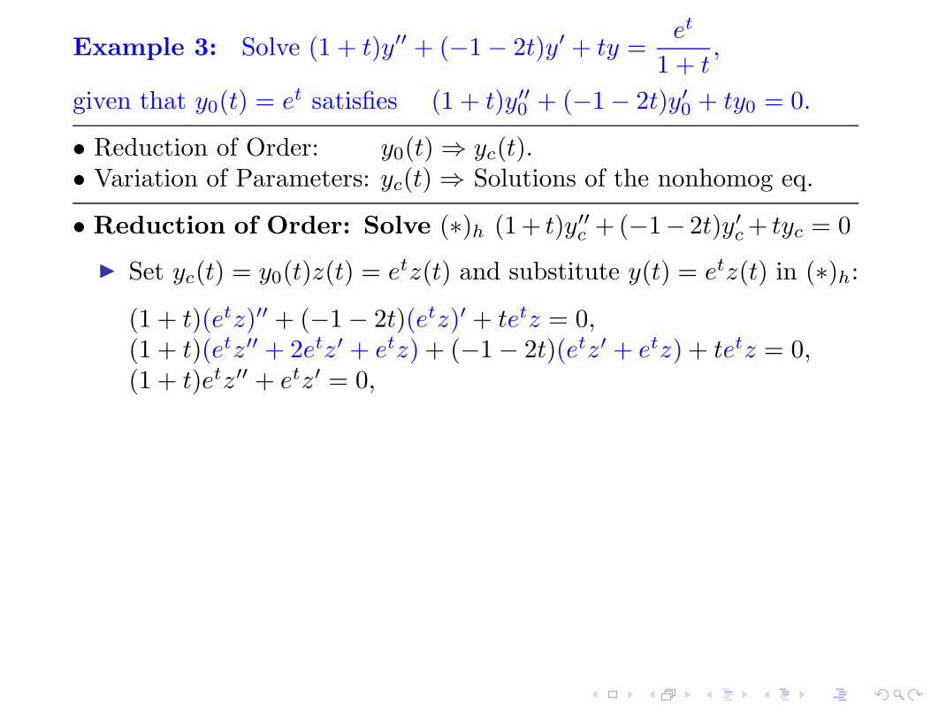
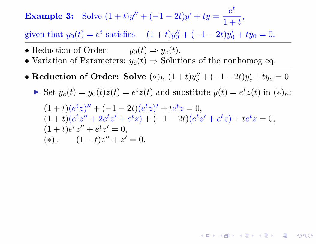
◮ Set yc(t) = y0(t)z(t) = etz(t) and substitute y(t) = etz(t) in (∗)h:
(1 + t)(etz)′′ + (−1 − 2t)(etz)′ + tetz = 0,
(1 + t)(etz′′ + 2etz′ + etz) + (−1 − 2t)(etz′ + etz) + tetz = 0,
Example 3: Solve (1 + t)y′′ + (−1 − 2t)y′ + ty =et
1 + t,
given that y0(t) = et satisfies (1 + t)y′′0 + (−1 − 2t)y′
0 + ty0 = 0.
• Reduction of Order: y0(t) ⇒ yc(t).• Variation of Parameters: yc(t) ⇒ Solutions of the nonhomog eq.
• Reduction of Order: Solve (∗)h (1+ t)y′′c +(−1− 2t)y′
c + tyc = 0
◮ Set yc(t) = y0(t)z(t) = etz(t) and substitute y(t) = etz(t) in (∗)h:
(1 + t)(etz)′′ + (−1 − 2t)(etz)′ + tetz = 0,
(1 + t)(etz′′ + 2etz′ + etz) + (−1 − 2t)(etz′ + etz) + tetz = 0,
(1 + t)etz′′ + etz′ = 0,
(∗)z (1 + t)z′′ + z′ = 0.

Example 3: Solve (1 + t)y′′ + (−1 − 2t)y′ + ty =et
1 + t,
given that y0(t) = et satisfies (1 + t)y′′0 + (−1 − 2t)y′
0 + ty0 = 0.
• Reduction of Order: y0(t) ⇒ yc(t).• Variation of Parameters: yc(t) ⇒ Solutions of the nonhomog eq.
• Reduction of Order: Solve (∗)h (1+ t)y′′c +(−1− 2t)y′
c + tyc = 0
◮ Set yc(t) = y0(t)z(t) = etz(t) and substitute y(t) = etz(t) in (∗)h:
(∗)z (1 + t)z′′ + z′ = 0.
◮ Set w(t) = z′(t). The eq (∗)z becomes a 1st order linear eq:
(∗)w (1 + t)w′ + w = 0.
◮ Solve (∗)w ⇒ w(t) =C1
1 + t.
◮ z′ = w ⇒ z(t) =∫
w(t)dt =∫ C1
1 + tdt = C1 ln |1 + t| + C2
◮ yc(t) = y0(t)z(t) = etz(t) = et [C1 ln |1 + t| + C2].
Or, equivalently, yc(t) = C1et ln |1 + t| + C2e
t.

Example 3 (continued): (1 + t)y′′ + (−1 − 2t)y′ + ty =et
1 + t.
• Reduction of Order: y0(t) = et ⇒ yc(t) = C1et ln |1 + t| + C2e
t.
• Variation of Parameters: yc(t) ⇒ Solve the nonhomog eq.

Example 3 (continued): (1 + t)y′′ + (−1 − 2t)y′ + ty =et
1 + t.
• Reduction of Order: y0(t) = et ⇒ yc(t) = C1et ln |1 + t| + C2e
t.
• Variation of Parameters: yc(t) ⇒ Solve the nonhomog eq.
◮ yc(t) gives a fundamental matrix:
M(t) =
[
y1 y2
y′1 y′
2
]
=
[
et ln |1 + t| et
et ln |1 + t| + et
1+tet
]

Example 3 (continued): (1 + t)y′′ + (−1 − 2t)y′ + ty =et
1 + t.
• Reduction of Order: y0(t) = et ⇒ yc(t) = C1et ln |1 + t| + C2e
t.
• Variation of Parameters: yc(t) ⇒ Solve the nonhomog eq.
◮ yc(t) gives a fundamental matrix:
M(t) =
[
y1 y2
y′1 y′
2
]
=
[
et ln |1 + t| et
et ln |1 + t| + et
1+tet
]
◮ ~x =
[
x1
x2
]
=
[
y
y′
]
satisfies ~x ′ = A(t)~x +
[
0et
(1+t)2
]
.
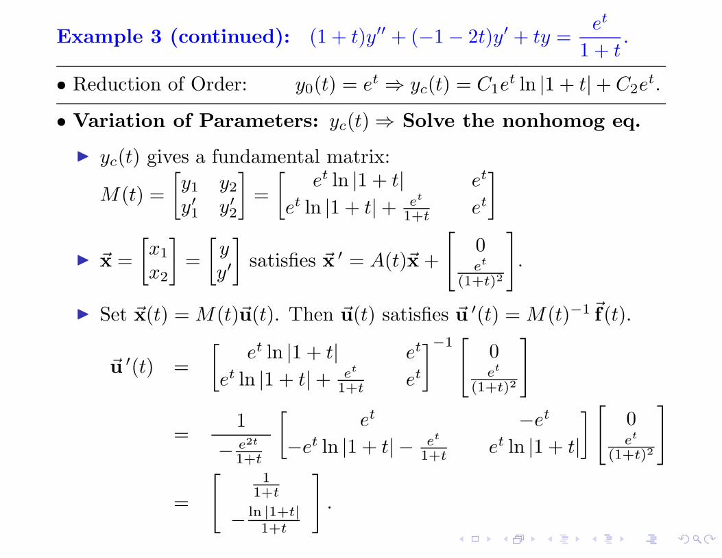
◮ Set ~x(t) = M(t)~u(t). Then ~u(t) satisfies ~u ′(t) = M(t)−1~f(t).
~u ′(t) =
[
et ln |1 + t| et
et ln |1 + t| + et
1+tet
]−1[
0et
(1+t)2
]
=1
− e2t
1+t
[
et −et
−et ln |1 + t| − et
1+tet ln |1 + t|
]
[
0et
(1+t)2
]
=
[
11+t
− ln |1+t|1+t
]
.
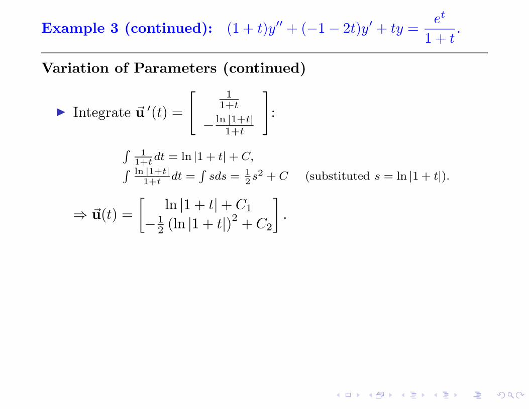
Example 3 (continued): (1 + t)y′′ + (−1 − 2t)y′ + ty =et
1 + t.
Variation of Parameters (continued)
◮ Integrate ~u ′(t) =
[
11+t
− ln |1+t|1+t
]
:
R
1
1+tdt = ln |1 + t| + C,
R ln |1+t|1+t
dt =R
sds = 1
2s2 + C (substituted s = ln |1 + t|).
⇒ ~u(t) =
[
ln |1 + t| + C1
− 12 (ln |1 + t|)2 + C2
]
.

Example 3 (continued): (1 + t)y′′ + (−1 − 2t)y′ + ty =et
1 + t.
Variation of Parameters (continued)
◮ Integrate ~u ′(t) =
[
11+t
− ln |1+t|1+t
]
:
R
1
1+tdt = ln |1 + t| + C,
R ln |1+t|1+t
dt =R
sds = 1
2s2 + C (substituted s = ln |1 + t|).
⇒ ~u(t) =
[
ln |1 + t| + C1
− 12 (ln |1 + t|)2 + C2
]
.
◮ Finally, we can get ~x(t) = M(t)~u(t) and y(t) = x1(t):
y(t) = u1(t)et ln |1 + t| + u2(t)e
t
= ln |1 + t| · et ln |1 + t| − 12 (ln |1 + t|)
2· et
+C1et ln |1 + t| + C2e
t
= 12et (ln |1 + t|)
2+ C1e
t ln |1 + t| + C2et.