December 1990 Report No. STAN-CS-90- 1345

Nonholonomic Motion Planning versus Controllabilityvia the Multibody Car System Example

Jean-Paul Laumond

Department of Computer Science

Stanford University

Stanford, California 94305

Nonholonomic Motion Planning versus Controllability via theMultibody Car System Example

Jean-Paul Laumond *

Robotics LaboratoryDepartment of Computer Science

Stanford University, CA 94305

(Working paper)Abstract

A multibody car system is a non-nilpotent, non-regular, triangularizable and well-controllablesystem. One goal of the current paper is to prove this obscure assertion. But its main goal isto explain and enlighten what it means.

Motion planning is an already old and classical problem in Robotics. A few years ago a newinstance of this problem has appeared in the literature : motion planning for nonholonomicsystems. While useful tools in motion planning come from Computer Science and Mathematics(Computational Geometry, Real Algebraic Geometry), nonholonomic motion planning needssome Control Theory and more Mathematics (Differential Geometry).

First of all, this paper tries to give a computational reading of the tools from DifferentialGeometric Control Theory required by planning. Then it shows that the presence of obstaclesin the real world of a real robot challenges Mathematics with some difficult questions whichare topological in nature, and have been solved only recently, within the framework of Sub-Riemannian Geometry.

This presentation is based upon a reading of works recently developed by Murray and Sastry[39], Lafferiere and Sussmann [55], and Bellaiche, Jacobs and Laumond [5] [33].

*On leave from Laas/Cnrs. His stay at Stanford was funded by DARPA/Army contract DAAA21-89-C0002.Permanent address : Laas/Cnrs, 7 Avenue du Colonel Roche, 31077 Toulouse, France. e-mail : jpl@laas.laas.fr

1

Contents

1 Introduction 4

2 From Planning to Control 7

3 The Modeling of a Multibody Car System 9

3.1 Geometric Model . . . . . . . . . . . . . . . . . . . . . . . . . . . . . . . . . . . . . . 9

3.2 Differential Model . . . . . . . . . . . . . . . . . . . . . . . . . . . . . . . . . . . . . 10

3.3 Control Models . . . . . . . . . . . . . . . . . . . . . . . . . . . . . . . . . . . . . . . 12

3.3.1 The Convoy is Driven by Gofer . . . . . . . . . . . . . . . . . . . . . . . . . . 12

3.3.2 The Convoy is Driven by Hilare . . . . . . . . . . . . . . . . . . . . . . . . . . 13

3.3.3 The Convoy is Driven by a Real Car . . . . . . . . . . . . . . . . . . . . . . . 13

3.3.4 The Convoy is Oddly Driven . . . . . . . . . . . . . . . . . . . . . . . . . . . 14

4 From Control to Planning : a Computational Point of View 16

4.1 What is the Problem ? . . . . . . . . . . . . . . . . . . . . . . . . . . . . . . . . . . . 16

4.2 A Controllability Algorithm . . . . . . . . . . . . . . . . . . . . . . . . . . . . . . . . 17

4.2.1 Phillip Hall Families . . . . . . . . . . . . . . . . . . . . . . . . . . . . . . . . 18

4.2.2 The Algorithm . . . . . . . . . . . . . . . . . . . . . . . . . . . . . . . . . . . 19

4 . 3 GrowthVector . . . . . . . . . . . . . . . . . . . . . . . . . . . . . . . . . . . . . . . 21

4.4 Singularities and Regular Systems . . . . . . . . . . . . . . . . . . . . . . . . . . . . 22

4.5 Well-Controllability . . . . . . . . . . . . . . . . . . . . . . . . . . . . . . . . . . . . . 22

4.6 Geometric Models and Singularities : some Examples . . . . . . . . . . . . . . . . . . 24

4.7 Nilpotent and Nilpotentizable Systems . . . . . . . . . . . . . . . . . . . . . . . . . . 25

4.8 Triangular Systems . . . . . . . . . . . . . . . . . . . . . . . . . . . . . . . . . . . . . 26

5 The Multibody Car System is Well-Controllable 28

6 The Complete Problem 30

6.1 From Vector Fields to Trajectories . . . . . . . . . . . . . . . . . . . . . . . . . . . . 30

6.2 Obstacle Avoidance : the Topological Question . . . . . . . . . . . . . . . . . . . . . 32

6.2.1 What Kinds of Topologies ? An Informal Statement . . . . . . . . . . . . . . 32

6.2.2 Of Sub-Riemannian Metrics, Shortest Paths and Geodesics . . . . . . . . . . 32

2

6.2.3 Geodesics and Shortest Paths : Elementary Computational Aspects . . . . . 34

6.3 A Planner Using Philipp Hall Coordinate Systems . . . . . . . . . . . . . . . . . . . 34

6.4 A Planner Using Shortest Paths. . . . . . . . . . . . . . . . . . . . . . . . . . . . . . 35

6.5 Complexity of the Complete Problem . . . . . . . . . . . . . . . . . . . . . . . . . . . 36

7 Appendix 1 : Related Work and Background 43

7.1 Car-like and Trailer-like Robots . . . . . . . . . . . . . . . . . . . . . . . . . . . . . . 43

7 . 2 SmoothPaths. . . . . . . . . . . . . . . . . . . . . . . . . . . . . . . . . . . . . . . . 43

7.3 Shortest Paths . . . . . . . . . . . . . . . . . . . . . . . . . . . . . . . . . . . . . . . 44

7.4 Time-Optimal Paths . . . . . . . . . . . . . . . . . . . . . . . . . . . . . . . . . . . . 44

7.5 Control-Oriented Approaches . . . . . . . . . . . . . . . . . . . . . . . . . . . . . . . 44

8 Appendix 2 : The 2- and &Body Car Systems 46

9 Appendix 3 : Proof of the Lemma in Section 5. 49

1 Introduction

The motion planning problem (MP) is certainly one of the best formulated ones in Robotics. Itraises two questions :

l Can a robot reach a given goal while avoiding the obstacles of its environment ? This is thedecision problem.

l If the answer to the previous question is yes, what path may it follow ? This is the completeproblem.

The geometric formulation of this problem is known as the piano mover problem. This formu-lation considers the motion of rigid bodies amidst obstacles in the 3-dimensional Euclidean space.The placement (translation and rotation) of a body in the Euclidean space is given by a point ina 6-dimensional space. Some geometric relationship between the bodies may appear for a givenrobotic system (as is typical for a robot arm). They are translated into equations between theplacement parameters of the bodies. These are called the holonomic links. They restrict the spaceof the allowed placements to a subspace of the placement spaces of all the bodies. This subspaceis called the configuration space. Finally, a configuration of the robot is represented by a point ofthe configuration space that defines precisely the domain occupied by the robot in Euclidean space.A point-path in the configuration space corresponds to a motion of the robot. For a holonomicsystem, we have as many degrees of freedom as is needed to follow any path.

Therefore, for holonomic systems, the existence of a collision-free trajectory is characterized bythe existence of a connected component in the admissible (i.e., collision-free) configuration space. Tosolve MP, it is enough to compute the admissible configuration space (i.e., transform the obstaclesin the Euclidean space into “obstacles” in the configuration space), and then explore its connectedcomponents.

Since the seventies this problem has attracted many researchers working in Robotics and beyond,in Computational Geometry and Algebraic Geometry. See [48] for a recent overview, [60] for areview of the various approaches of the problem, and [27] as the first genuine book on the subject .

However, there are cases in which this formulation of motion planning is not sufficient. In thelast four years, an example of the limitation of the piano mover formulation has been investigated :planning constrained motions where constraints are nonholonomic in nature. A nonholonomic linkis expressed as a non-integrable equation involving derivatives of the configuration parameters.Such constraints are expressed in the tangent space at each configuration; they define the allowablevelocities of the system, and they cannot be eliminated by defining a more restricted configurationspace manifold. Thus, the main consequence of a nonholonomic constraint is that an arbitrarypath in the admissible configuration space does not necessarily correspond to a feasible trajectoryfor the robot. Therefore, the existence of a collision-free trajectory is not a priori characterized bythe existence of a connected component in the admissible configuration space.

Planning motions for nonholonomic systems is not as new in other communitiescommunity working on obstacle avoidance for robotsr. This problem is well known in

as in theNonlinear

‘Notice that nonholonomic motion planning appears also in some spatial applications, forstations or satellite) using internal motion and submitted to conservation laws (see [40] [42]).

systems (like space-

4

Control and in Differential Geometry. Important results have been obtained over the last twodecades, while the first results seem dated from the thirties with Chow’s work [12].

Notwithstanding, Robotics brings to the front an important constraint which is not usually takeninto consideration : the planner has to produce trajectories that avoid the obstacles. Moreover, byits applications to the real world, it requires effective and efficient computational tools, rather thanjust proofs of existence.

Results useful to our problem can be found in publications-often difficult ones-from othercommunities than the Robotics one. Because the viewpoints are different, they at tack only someaspects of the problem, and use different terminologies. The goal of this paper is to enlightenthese points of view by a computational one (the right point of view for the planning problem)and to stress the connections between motion planning and differential geometric control theory.This study has to be viewed as an informal statement of these connections, hopefully readableby a non-specialist in control theory or in differential geometry (as the author is). A spotlightwill be focused on some concepts from these theories, using a minimal formalism while trying tounderstand where and why these are pertinent as far as the motion planning problem is concerned.It is clear that an in-depth study of these concepts needs the precision given by the mathematicalformalism : for each concept there will be references introducing or using it.

Along this study we take a multibody car system (i.e., like a luggage carrier in an airport) asan example of application. The results (Section 3 and Section 5) for this example constitute acontribution by themselves. They can be read independently of the rest.

The decision problem of planning for nonholonomic systems is related to their controllability2 :more precisely the existence of a collision-free trajectory for a controllable nonholonomic robotis characterized by the existence of an open connected component of the admissible configurationspace. The decision problem is then similar to that of the piano mover problem. This resultconstitutes the first main link; it has been studied simultaneously in several research groups : [31][34] [3] [38]. It is based upon the Lie algebra rank condition, and will be recalled in Section 2.

Section 3 presents a three-step modeling of the multibody car system, from a purely geometricmodel leading to the definition of the configuration space (Section 3.1), to four distinct controlmodels, all corresponding to practical applications (Section 3.3), via a differential model (Section3.2). The differential model finally enables us to give a unified proof of controllability encompassingall the envisaged systems (Section 5).

Section 4 refines the presentation of Section 2, by considering the computational aspects of theproblem : is a system controllable ? There is a semi-decidable procedure for this problem, which issupported by several concepts of differential geometric control theory. Then this paper introducesthe well-controllability notion, in relation to the planning problem.

Nevertheless, at this stage the complete problem of nonholonomic motion planning remainsunsolved.

5

Section 6 considers the complete problem. We will see that the key question is topological innature. While motion planners for nonholonomic systems have blossomed through the last twoyears (see Appendix l), very recent contributions pursue a deep study of the differential geomet-ric tools available for solving the complete problem. [33] p resents an efficient planner for mobilerobots and shows that its strategy can be generalized. [55] presents a general planner based upona general constructive proof of controllability. These results let us stress the main difficulty forbuilding efficient planners : while obstacle avoidance requires us to consider the “natural” Rieman-nian topology of the configuration space (i.e., induced by the natural Hausdorff metric workingin the robot environment), the trajectories allowed by the nonholonomic constraints compel usto consider another topology in this space : the topology induced by the length of the shortestallowed path between two points. Such a metric is known as a sub-Riemannian (or singular, orCarnot-Caratheodory) metric. In fact, using sub-Riemannian geometry (see [7] [51] [58] [36]), itis possible to show that both topologies are the same. This result enables us to conclude on thegenerality of the approaches presented in [33] and [55]. Nevertheless, because we are interested inthe computational point of view, we have to study more deeply the shape of the sub-Riemannianmetrics in order to estimate the combinatorial complexity of the planners. This study has beendone in [33] for the case of the car-like robot. This section points at the reference [58] that givesprecisely the general and finest form of the sub-Riemannian metric we need to conclude on thecomplexity of the complete problem.

Appendix 1 overviews other results related to nonholonomic motion planning : they do notuse intensively the tools we present in this paper, but they are interesting nonetheless from eithera theoretical or a practical point of view. Following appendices give the various computationsfor the examples presented along the paper (Appendix 2), together with the tedious proof of thecontrollability result presented in Section 5 (Appendix 3).

Two starting points are at the origin of this working paper. The first one has been the work ofBarraquand and Latombe on the controllability of multibody systems (see [4]). This report yieldsa proof of controllability in a general case involving up to n trailers. The second point has been areading of papers written by Murray and Sastry [38] [39] and by Lafferiere and Sussmann [55]. Itseemed interesting to clarify the relationship between these approaches of the planning problem,taking also into account the approach ([30] [33]) developed within the Hilare mobile robot project[16] [lo] by Jacobs and the author.

2 From Planning to Control

Until a very recent period, the main contribution to nonholonomic motion planning (independentlydeveloped in [31] and [34]) has been to solve the decision part of the nonholonomic motion plan-ning problem, via differential geometry and control theory. See [3] for a clear presentation of thenecessary tools that we examine here.

While the constraints due to the obstacles are expressed directly in the manifold of configura-tions, nonholonomic constraints deal with the tangent space. In the presence of a link between therobot’s parameters and their derivatives, two questions arise :

l Is this link holonomic ? (i.e., does it reduce the dimension of the configuration space ?)

l If not, does it reduce the accessible configuration space ?

In the case of r links corresponding to r equations linear in the derivatives of the n parameters,these equations determine what is called an (n- r)-distribution A on the manifold of configurations.The answer to the first question is then given by Frobenius’ theorem (see for instance [49]): theequations are integrable if and only if the distribution A is closed under the Lie bracket operation.Let us recall that the Lie bracket of two vector fields X and Y is defined as [X, Y] = 8X.Y - dY.X.A sample of computation examples appears in Appendix 2.

From a control theory perspective, a control is a function which allows us to choose the systemstate velocity at each instant by a careful weighting of smooth vector fields. The control Lie algebraassociated with A, denoted by LA(A), is the smallest distribution which contains A and is closedunder the Lie bracket operation. The answer to the second question is then given by the non-linearsystem controllability theorem (see for instance [53] [35] [17]): if the rank of the Lie algebra isfull at a given configuration c, then there exists a neighborhood N of c whose points representconfigurations reachable by the system moving from c along an admissible path. Moreover, thispath stays in N. This condition is known as the “rank condition”; it is a local condition.

If the rank condition holds everywhere in the configuration space, then the robot is termedcon trolla ble 3. From our planning point of view, the main consequence is that the existence of acollision-free trajectory is characterized by the existence of a connected component in the free (i.e.,with neither collision nor contact) configuration space.

Therefore, apart from topological subtleties dealing with motions in contact, the decisionproblem of motion planning for controllable systems is the same as for holonomicones4.

The difference is more involved with the complete problem. The previous result answers thequestion of the existence of a feasible trajectory, that is, the decision problem, but does not solve the

31n fact a controllable system requires only that the rank condition holds nearly everywhere, that is on a densesubset of the manifold. Various precise controllability concepts appear involving the “size” of reachable sets and the“size” of sets where the rank condition holds (see [54]). Omitting them does not affect our purpose.

‘Section 3 highlights the difficulty for proving the controllability of a system. Since we are interested in thecomputational point of view, we are looking for a procedure that allows us to conclude. As we will see, this problemis not trivial.

problem of efficiently producing an admissible trajectory. To the extent of the author’s knowledge,there was no general constructive proof of the result mentionned above until the recent contributionof Lafferiere and Sussmann [5515. Their proof leads to the design of a general nonholonomic motionplanner in the absence of obstacles (see Section 6).

At this stage we can just hope that the search for a solution for a nonholonomic system canbe guided by a collision-free trajectory for the associated holonomic system. Indeed, thanks to thelocal property above, a controllable robot can be steered close to any path as long as there is a“small gap” between the reference path and the obstacles. This idea is precisely the basis of thetwo strategies defined in [55] and [33] that we will study in Section 6. It appears clearly that thekey question for developing such a strategy deals with the size of the “gap”, i.e., with the topologyinduced by the nonholonomic constraints. This aspect is detailed in Section 6.

Now let us define the multibody car system.

5Specific constructive proofs appear in [28] for the car-like robot and in [32] for the car-like robot pulling a trailer.

8

3 The Modeling of a Multibody Car System

Figure 1 shows what we call a multibody car system. It corresponds to a car-like robot pullingand pushing trailers (like a luggage carrier in an airport). In order to grasp the planning pointof view, we will build along three modeling levels for this system : a geometric model (Section3.l), a differential model (Section 3.2) and a control model (Section 3.3) respectively. Then aclose examination shows that four different control systems correspond to the same differentialmodel; this is the differential model that we will use to solve the decision part of the planningproblem (Section 5).

Figure 1: A multibody car system

3.1 Geometric Model

Let us consider a multibody system (Be, Br, . . . , f3,> constituted by a car f?e and n trailers B;. Wetake the midpoint between the rear wheels as the reference point for each body; its coordinates are

9

denoted by x; and y; in some fixed Cartesian frame of the plane; the angle 8; is taken between themain axis of .13; and the x-axis of the frame. The space of possible placements of the n + 1 bodiesis then 3(n + 1)-dimensional.

In order to form a convoy (e.g., the car pulling the n trailers B;, each hooked up to the nextlike for a luggage carrier), each trailer L?; is assumed to be hooked up to the midpoint between therear wheels of the preceding body f?;-r 6. This means that the system is submitted to 2n holonomiclinks which yield the following equations in the placement space7 :

Xi -Xi-l = -case;,

Yi - y;-1 = -sine;.

The configuration space of the convoy is a submanifold of dimension 3(n + 1) - 2n = n + 3 in theplacement space of all the bodies. A possible parameterization of this submanifold is to pick outthe (n + 3)-tuple (x0, yn, 80,8r, . . . ,B,) belonging to R2 x (S’)n+l. For the sake of simplicity, wewill set x = x0, y = yo, 0 = e. and cp; = 8; - &-I, so that p; is the angle between the axes of B;and Bi-1, and use (x,y,Ql, . . . , cpn) as an alternative parameterization.

3.2 Differential Model

Each body is rolling on the ground without sliding; thus it is submitted to the classical nonholonomiclink :

ii sin 8; - ~j; cos ei = 0.

Remark : This equation is obvious. We just want to mention the following fact : it has beenobtained without any reference to a control system; we have just used some elementary kinematicconsiderations (i.e., a moving rigid body has only one instantaneous center of rotation).

The system is subject to n + 1 such constraints. Since the number of degrees of freedom of amechanical system is defined as the difference between the dimension of its configuration space andthe number of independent nonholonomic links, the number of degrees of freedom of our convoy is(n + 3) - (n + 1) = 2 (obviously, the 2 degrees of freedom of the car. . . ).

These constraint equations are expressed in the tangent space of the placement space of all thebodies. In order to translate them into the tangent space of the configuration space, we have to getrid of the variables i; and jl; for i # 0’ . By combining these n + 1 equations with the derivativesof the 2n holonomic equations, we obtain the following system of n + 1 linear equations :

i0 sin 8; - $0 cos 8; - C ij cos(Bj - 0;) = 0.j=l

A configuration c being given, this system defines a plane in the tangent space at this point; thismeans that, for a possible motion passing through c, the velocity vector at c-whenever defined-has to lie in that plane8. If we compute the solution of the resulting system, we obtain :

‘The hooking system is important. The equations do not simplify if the trailers are hooked behind the rear axles.-Moreover the problem is unsolved for this generalization.

7We assume that all the links have the same length 1; obviously, this does not affect the generality of the followingresults.

‘The set of all these planes has the structure of what is called a distribution on the manifold.

10

i0 = a cos 80$0 = a sin 00e, = p.

01 = ct sin(81 - e,).

e2 = 0 cOs(el - eo) sin(& - e,)

e, = a sin@, - 0,-l) n$ cos(8; - 9i-1)i=l

with cy and p any two reals. Setting ((Y, /3) = (1,0) and (cr, /3) = (0,l) yields a basis of the plane,namely :

-L = (cOseo, sineo, 0, sin(& - e,), cOs(el - e,j sin(& - e,), . . .n - l

-** 7 sin(8, - On-l> n cOs(oj - 8,-l)),j=l

Xb = (0, 0, 1, 0, . . . ,o).

If we use the change of variable pi = 0; - Oi-1, the same computation yields9 :

2 = cx cos 0

j, = asines = p

+1 = p-crsincpl

$52 = cx (sin ‘p1 - cos $01 sin 92)

$53 = a cos 91 (sin (p2 - cos +92 sin p3 j

.n - 2

.Pn = (Y (sin (Pn-l - COS (Pn-1 sin pn) n COS Cpi

i=l

as the parameterized equations of the plane, and

x, = (cos0, sin 0, 0, - sinql, sin91 - cosvl sin+92, . . .n - 2

. . . , (sin+9,-1 - COS (Pn-1 sin Cpn) I-J COS Pj) 7j=l

& = 0, 0, 1, 1, 0, . . .

Unfortunately the general shape appears only from the 6th coordinate

11

as a distinguished basis.

Recall that all this system modeling has been done without reference to any control system.It has been built just from the non-sliding hypothesis applied to each body of the convoy. So anycontrol system will apply to the framework above. We will use the generality of the differentialmodel in order to prove the controllability of the convoy for several control systems.

3.3 Control Models

At this moment, we have not mentioned yet how the system moves. We have just suggested thatthe first body drives the convoy. But we can imagine that the car is in the middle of the convoy;better it may be possible that there is no car, and just some effecters controlling the angularjoints between the bodies (as in some japanese snake-robots). We examine here four examples ofcontrol systems and prove that, in all cases, the proof of controllability of these systems amountsto computing exactly the same Lie algebra, namely the Lie algebra spanned by the vector fields X,and Xb introduced above.

3.3.1 The Convoy is Driven by Gofer

The Stanford mobile robot Gofer [ 1 l] is very interesting for our purpose. Indeed it leads to intro-ducing a distinction between the control variables and the parameters which is pertinent from thepoint of view of the planning. Gofer’s locomotion system is clever : three parallel driving wheelsare linked together by some mechanical system; their velocities are controlled by a same motor(which produces forward or backward motions), while a second motor can control their directions.Such a design requires that there be a part of the vehicle whose direction remains fixed.

If the non-rotating part has a geometric shape whose projection on the plane contains theprojection of the whole robot, then the robot appears, from the planning point of view, as atranslating, but non-rotating body. In this case the reference frame of the robot is linked to thefixed part and the configuration space is only 2-dimensional.

Otherwise, if the projection of the non-rotating part is included in the projection of the otherparts, the robot appears (always from the planning point of view) as a 2-dimensional translatingand rotating body. The configuration space is thus 3-dimensional. The robot looks closely likewhat is called a unicycle : this means that the speed of the vehicle and its direction are directlycontrolled by two independent motors”.

Therefore, with (x, y, 0) designating a configuration of the robot, the control system is :

“The distinction we have introduced is meaningless for the true robot, since Gofer is circular ! However, this isan example of the subtle links that may appear between a geometric model for planning and a differential model forcontrol : think of the case where none of the projected parts would be included in the other; in that case the planningproblem would concern a translating, rotating and deformable 2-dimensional body. As a matter of fact, Gofer is but apretext to introduce the interesting case of the unicycle. . . And, in order to be exhaustive with the Stanford RoboticsLaboratory, there is also a robot called Mobi whose sophisticated locomotion system endows with the privilege ofbeing one of the few existing holonomic mobile robots.

12

(34 :i++( gu2.

Thus if we attach 12 trailers at Gofer’s rear its control system expresses directly as the two vectorfields X, and Xb defined in the preceding section, so that the controllability of the system will beestablished by computing the Lie algebra spanned by {X,, Xb}.

3.3.2 The Convoy is Driven by Hilare

Consider now the Hilare family, dwelling at Laas [16] [lo]. The three mobile robots have the sameclassical locomotion system : two parallel driving wheels, the acceleration of both being controlledby two independent motors. Assume that the distance between the wheels is 2, that the referencepoint of the robot is the midpoint of the wheels and that the main direction of the vehicle is thedirection of the wheels. With ~1 and ~12 as their respective speeds, the control system is :

In fact, from the planning point of view that we take in this paper ;he speed at a configuration isnot considered as a part of the problem), this system can be rewritten in the following way :

If we add the trailers, the vector fields corresponding to the controls are clearly Y, = X, + Xband Yb = X, - Xb. In order to prove the controllability of the convoy we have to compute thedimension of the Lie algebra spanned by {Y,, Yb}. Due to the bilinearity of the Lie bracket, it isequivalent to start with {X,, Xb}.

3.3.3 The Convoy is Driven by a Real Car

The case of a real car is a little bit more complicated. Indeed, in addition to the nonholonomic link,a specific constraint appears : the turning radius is lower bounded (we will see that this constraintdoes not cause any trouble).

From the driver point of view, a car has two degrees of freedom : the accelerator and the steeringwheel (the brake is a kind of reverse accelerator and the clutch pedal is reserved to European

13

drivers . . . ). Take the midpoint of the rear wheels as the reference point. Assuming that thedistance between the rear and the front axle is 1, we denote by v the speed of the car and by cp theangle between the front wheels and the main direction of the car rl. Simple arguments show thatthe control system is the following :

[ i)=( y!?j+( #+[ gu2.

Again we are only interested in the geometric planning problem. Then, since the position of thefront wheels is not relevant to the problem, as well as the speed of the vehicle, the system simplifiesinto :

(S) = (Ef$cos~+( +sin+2

This is a non-linear system whose controls are w and 9. Anyway, as shown by the form of theequation, if we add trailers, the controllability of the convoy will still be proven by a close study ofthe Lie algebra spanned by X, and Xb.

Remark : We did not take the constraint on the turning radius into account. This constraintcan be expressed as 191 < ve,where ‘pe is a strictly positive real. From the point of view ofthe complete control model, this constraint has exactly the same meaning as an obstacle in theenvironment (an obstacle in the environment constrains the variables x, y and 0 to lie in somedomain); therefore, it does not affect the controllability of the complete system and, consequently,it does not affect the controllability of the simplified system either12.

3.3.4 The Convoy is Oddly Driven

The following system is no longer classical. Unlike the previous ones the driver system does notinvolve the first body alone but also the second one. These bodies being articulated, a configurationwill be denoted by (x, y, 0, cp). The specificity of the system lies in its controls : the linear speedof the first body, and the angle cp between the bodies. This system actually corresponds to somevehicles used in civil engineering13.

“More precisely, the front wheels being not exactly parallel (else they would slide), we take the average of theirangles as the turn angle.

“Barraquand and Latombe [4] 1 be a orate on this point and take advantage of it to exhibit a motion planner that caneven manage constraints of the form 0 < cpr < cp 5 972 (i.e., the car can only turn right !); independently Bellaiche,Jacobs and Laumond give a proof in [5] for a Hilare-like system verifying ]vr ] 5 ]vz] ,e.g., equivalent to a car-likerobot: the vehicle turns (]vz] > 0) only if its linear speed is not zero (1~1 I > 0).

13R. Hurteau from Polytechnical Scholl of Montreal mentioned this example to the author: that kind of vehicle isused in the conveyance of ore in some Canadian salt mines.

14

Let ur be the speed control of the first body; let u2 be the control of the angular joint of thebodies. Since both are independent, ur is applied onto a vector field Ya = (cos 8, sin 0, a, 0) while u2is applied onto a vector field Yb = (O,O, b, 1). A 1c ose study of the differential model above (section3.2) leads us to find a = sin cp and b = 1. The control system is :

2

O(

cos 0 0i sin 8 04 = sin cp Ul + 1 u2*

+ 0 i 01

Therefore the system is controllable if the Lie algebra spanned by Y, and Yb is four-dimensional.Furthermore, Yb is equal to the vector field Xb instantiated with only one trailer. Moreover :

cos 8

Y, =sin 0

i 1sin cp

0.yiq [)00 t sincp l

- sin cp 1

= x, + sinpxb.

Hence, Y, ends up to be a linear combination of X, and Xb. The Lie algebra spanned by Ya and Ybis the same as the Lie algebra spanned by X, and Xb. These results obviously hold if we add trailersto this strange vehicle and the controllability of the convoy remains subject to the computation ofthe Lie algebra spanned by X, and Xb as in the previous cases.

Conclusion

The decision part of the planning problem for the four multibody systems above is the same. We justhave to study the distribution appearing in the differential model. This study appears in Section 5.We now discuss some computational aspects of the general tools we can use to achieve this.

15

4 From Control to Planning : a Computational Point of View

4.1 What is the Problem ?

Proving the controllability of an n-dimensional system using the rank condition involves showingthat, for any point c in the manifold, there exists a family of n vectors fields in the Control LieAlgebra that spans R” when applied to c. This stirs two difficulties due to the local and globalcharacteristics of the problem :

l At any specific point c, finding such a family enables us to conclude. Not being able to finda suitable family does not imply that there is none. An exhaustive enumeration of possiblefamilies is impossible since there is an infinity of potential choices. We will see (Section 4.2)that this number can be reduced to a countable one, but not further, leading to the design ofsome semi-decidable procedures. We will proceed then to giving an estimate of the complexityof procedures testing the controllability of a system at a point.

l One may succeed in finding bases that work somewhere, but not necessarily everywhere. Theremay be some singularities. An interesting problem is to know whether such singularities havean intrinsic nature, or depend upon the choice we make (Sections 4.4 and 4.6).

As far as we know, testing controllability is not a decidable problem. Nevertheless, the procedurewe define always terminates provided we don’t encounter any singularities (Sections 4.7 and 4.8).

The material of this section uses the concepts of a distribution, also known as a Pfaffian system(see for instance [58]), and of the Free Lie Algebra (see [S]).

Let us recall that every Lie operator has to verify skew-symmetry [X, Y] = -[Y, X] and theJacobi identity [X, [Y, Z]] + [Y, [Z, X]] + [Z, [X, Y]] = 0.

Consider the (n - r)-distribution A associated with a robotic system. We want to define analgorithm for testing the controllability of that system at a point. Precisely, we are interested inthe rank of LA(A) ( i.e., the distribution spanned by all the combinations of Lie brackets of vectorfields in A). We can consider a basis X of A together with all the combinations of Lie bracketsbuilt upon that basis.

To do this, one may consider a brute force strategy consisting in building iteratively the followingincreasing sequence of distributions : Ai = Ai-1 + [Ai-,, A;-r] where [A;-,, A;-r] is the linearspace spanned by all the brackets [X, Y] for X and Y in A;-,. By putting A = A,, the ControlLie Algebra LA(A) pis recisely defined as Ui Ai. But in fact, a more efficient strategy can be used.First of all, let us define a parameter estimating the complexity of a combination of Lie brackets.The degree of a combination is the number of elements in X defining the combination. For examplethe degree of [. , [. , [. , .]], [. , [. , .I]] is 7. Now, our strategy will consist in building all the brackets ofa given degree, step by step. This strategy is founded on the following iterative construction. Wedenote A by A,. Then Ai is defined by :

Ai = k-1 t C [Aj,Ak]-j+k=i

16

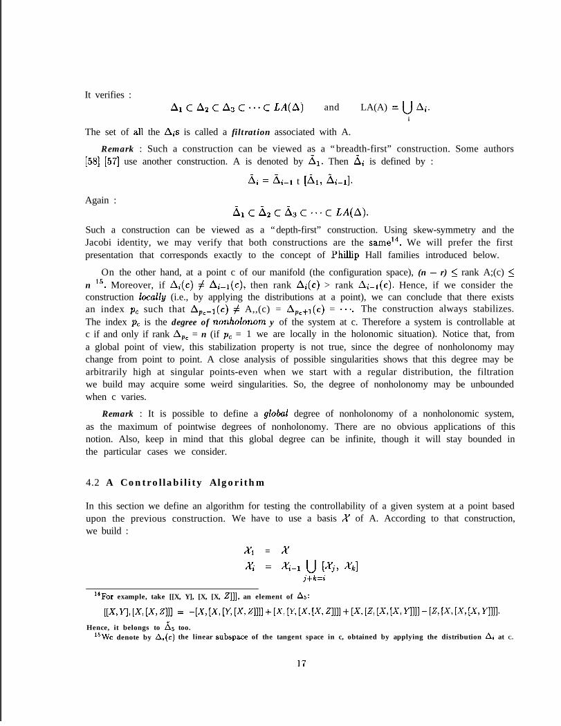
It verifies :&c&cA3c-~cLA(A) and LA(A) = U Ai.

i

The set of all the Ais is called a filtration associated with A.

Remark : Such a construction can be viewed as a “breadth-first” construction. Some authors[58] [57] use another construction. A is denoted by Ai. Then Ai is defined by :

lii = L&i-l t [Al) &-11.

Again :

Such a construction can be viewed as a “depth-first” construction. Using skew-symmetry and theJacobi identity, we may verify that both constructions are the same14. We will prefer the firstpresentation that corresponds exactly to the concept of Phillip Hall families introduced below.

On the other hand, at a point c of our manifold (the configuration space), (n - r) 5 rank A;(c) 5n 15. Moreover, if A;(c) # A;-,(c), then rank A;(c) > rank A;-r(c). Hence, if we consider theconstruction locally (i.e., by applying the distributions at a point), we can conclude that there existsan index p, such that Ap,_r(c) # A,,(c) = Ap,+i(c) = a... The construction always stabilizes.The index p, is the degree of nonholonom y of the system at c. Therefore a system is controllable atc if and only if rank Ape = n (if p, = 1 we are locally in the holonomic situation). Notice that, froma global point of view, this stabilization property is not true, since the degree of nonholonomy maychange from point to point. A close analysis of possible singularities shows that this degree may bearbitrarily high at singular points-even when we start with a regular distribution, the filtrationwe build may acquire some weird singularities. So, the degree of nonholonomy may be unboundedwhen c varies.

Remark : It is possible to define a global degree of nonholonomy of a nonholonomic system,as the maximum of pointwise degrees of nonholonomy. There are no obvious applications of thisnotion. Also, keep in mind that this global degree can be infinite, though it will stay bounded inthe particular cases we consider.

4.2 A Controllability Algorithm

In this section we define an algorithm for testing the controllability of a given system at a point basedupon the previous construction. We have to use a basis X of A. According to that construction,we build :

Xl = xXi = X-1 U [xj, xk]

j+k=i

“For example, take [[X, Y], [X, [X, Z]]], an element of AS:

[[X, Y], [X, [X -q]] = -[X [X [Y, [X, 4111+ K K K [X7 ~1111+ K K K K y3111 - K WY K K yl111~Hence, it belongs to &, too.

15We denote by A;(c) the linear subspace of the tangent space in c, obtained by applying the distribution Ai at C.

17

where, now, [Xj, &] is no longer viewed as a linear space, but as a finite family of brackets. EachXi contains of course a basis of Ai. Again, we can define the union U(X) of all theses familiesand we have :

Xl c X2 c X3 c l . - c LA(X)This is clearly an infinite family, but, during the real process, we can check out the added elementsif they happen to be linearly dependent on the previous ones.

Even if we know only about the relations pertinent to the concept of a Lie Algebra, we can takeadvantage of these to compute only relevant elements of what is called the Free Lie Algebra.

4.2.1 P hillip Hall Families

In this section l6 the elements of LA(X) are considered as formal expressions produced by theconstruction above, i.e., they are not actually evaluated as vector fields belonging to a distribution.From this point of view, LA(X) is considered as a Free Lie Algebra. Our current problem is toenumerate a basis of this algebra, i.e., to get rid of redundant elements using only skew-symmetryand the Jacobi identity. Such a basis can be found via a Phillip Hall family.

The degree of an element X in LA(X) is denoted by degree(X) : this is the degree of themonomial defining X 17. According ot our notations, a Phillip Hall family (PH-family for short)of U(X), is any totally ordered subset (W-t, 4) such that :

l If X E Px, Y E PB and degree(X) < degree(Y) then X 4 Y;

. XcP?i;l m7Xz = {[x,YI, x 4 Y);l An element X E LA(X) with degree(X) 2 3 belongs to 7% if and only if X = [U, [V, W]]

with U, V, W in P3t, [V,W] in P�F I, V 5 U 4 [V,W] and V 4 W.

The main property of a PH-family is that, taking skew-symmetry and the Jacobi identity intoaccount, it yields a basis of the free Lie algebra ,CA( X) [6].

The proof of existence of such a family is easy; it is an iterative one. In the context of ourcontrol problem, it can be extended into the following algorithm.

“The material used in this section comes from [6]. We want just to give a rough idea of the concept and of itspertinence with respect to our problem. Interested readers will find a more rigorous presentation in this reference.

l7 We use the word “degree” with two different meanings, according to whether we speak of a bracket or of anonholonomic system. This may introduce some confusion, but both terms are already used in the literature (see forinstance [57]).

18

4.2.2 The Algorithm

The idea is to build a PH-family, based upon a graded family of sets IFI;, where 3-1; is a part of Xi.We wilI also build a total order 4 on the union Ni. Assume first that X is totally ordered by < andset 7ii = X. The order 4 on tir is the same as the order < on X. The next set ‘FI;! is defined asthe set of all [X, Y], with X,Y elements of Ni and X 4 Y. Endow ti2 with any total order, anddefine 4 on tii U Ff2 by setting X 4 Y, for X in xi and Y in 1Fl2.

The rest of the algorithm consists in building the sets ‘Mi iteratively. Suppose the family‘Fll, 7f2, . . . , Xi-1 is given. Denote it as 7-1. Define wi according to the definition of a PH-family.That is, ?& is the set of all X = [U, [V, W]] verifying : U E ‘Mj, [V, W] E 7fi-j, V 5 U 4 [V, W] andV 4 W. Choose a total order on xi and extend it to ti U7-1; : X + Y if X E ‘FI and Y E ‘.Mi. It isalmost obvious that the family 7f.i is a PH-family and, furthermore, that the degree of an elementof ai is precisely i.

We can use this construction to design an algorithm for testing the controllability of a systemat a point c of the manifold. Our algorithm adds new brackets to the PH-family step by step, butnow, we check further the value of each new bracket as a potential member of a basis at c. If weultimately obtain a basis, the system is controllable at c.

In the following procedure, B denotes the free family that will eventually become a basis, cnt is thecurrent number of element of that basis. The initial distribution is (n - r)-dimensional at the point c. Foran order on ‘H, we assume that we have an initial order on X; then we simply take the order of chronologicalcomputation. Finally 1x is the integer part (floor function) of the real x.]

Procedure ControZlabiZi~y(c)(initialize 311)T-l1 txa txcnt 4- n - r(build 312)ForX,YinZl,X+Ydo

add [X, Y] in 7i2;If {[X, Y](c)} U B(c) is a free family (l)

thenadd [X, Y] in Bcnt + cnt + 1

it2While cnt < n do

iti+l(build 7-t;)For 1 5 j 5 L;/2] do

For X EZ~, Y = [U,V] E’Hi-j doIf u 5 x t2)

thenadd [X, Y] in 7&If {[X, Y](c)} U 23(c) is a free family t3)

thenadd [X, Y] in Bcnt t cnt + 1

1 9

One can verify that the procedure builds sets 3-1; defining a PH-family. Therefore, it appears clearlythat the system is controllable at c if and only if Controllability(c) terminates. This also meansthat the procedure never stops otherwise.

Example Part 1 : For a classical example [6] [55], take X = {Xi, X2). The first 14 elementsof the PH-family generated by the procedure (if it does not stop before) are:

X1 x3 = [xl, x2] x4 = [xl, [xl, x,]] & = [xl, [xl, [xl 3 x2111 xg = Lx1 ’ Ix,) Lx’) Ix” x21111x2 x5 = [X2, [Xl, X2]] x7 = [X2, [ X l , [ X l , x2]]] Xl0 = [X2> [Xl> [Xl, [Xl, x21111

X8 = [X, ) [X,, [XI, X2]]] x11 = [X2 9 1x2 3 [Xl 9 [Xl 9 x~llllx12 = [X2, [X2, [X2, [Xl > x21111x13 = [[Xl, x21, [Xl 7 [Xl, x2111x14 = [[Xl, x21 9 [X2, [Xl 9 x2111

Example Part 2 : Consider now the controllability aspect. Replace Xr and X2 by the vectorfields X, and Xb defining the nonholonomic distribution of the 2-trailer convoy (see Section 3.2).The configuration space is a 5-dimensional manifold. Let c be a point of coordinates (2, y, 6, ~1, (~2).Yields :

cos 8sin 9

x1 =

i I

0- sin cpr

sin ~1 - cos ‘pl sin cp2

The first elements of a PH-family are displayed in Example Part 1 (see Appendix 2 for the coordi-nates of the various vector fields). We can verify that the algorithm stops with {Xl, X2, X3, X4, X6)as a basis for every point c verifying cpi $ t mod 7r. The algorithm stops with {Xl, X2, X3, X4, X9}for the remaining hyperplane”.

Remark : Finally, the rank condition holds everywhere and we can conclude that the corre-sponding system is controllable.

In this example, notice that the algorithm checks 6 - 2 = 4 “candidates” in the first case, and9 - 2 = 7 in the second one. What happens in the general case ?

The core of the algorithm is the construction of a PH-family. The dimension n of the manifoldbeing a constant integer of our problem, the only tests needing a subroutine depending on n are (1)and (3). Their complexity is asymptotically negligible. Therefore the worst-case complexity of thealgorithm is dominated by the complexity of building a PH-family. The relevant parameter is thevalue of i when the algorithm stops. Because of the test (a), our procedure for building a PH-familyis not optimal lg . But, here, we just want to find the minimal complexity of any algorithm that

“More precisely : x5 = X1, det(X1, X2, X~,XI,XS} = -cos(q~), X7 = 0 , Xs = -X3 a n d f i n a l l ydet{X1,XS,X3,Xh,X9} = - 1 -cos2(~~)cos(~~).

lgIt seems possible to define an optimal one. Maybe such a procedure already exists in the literature ?

20

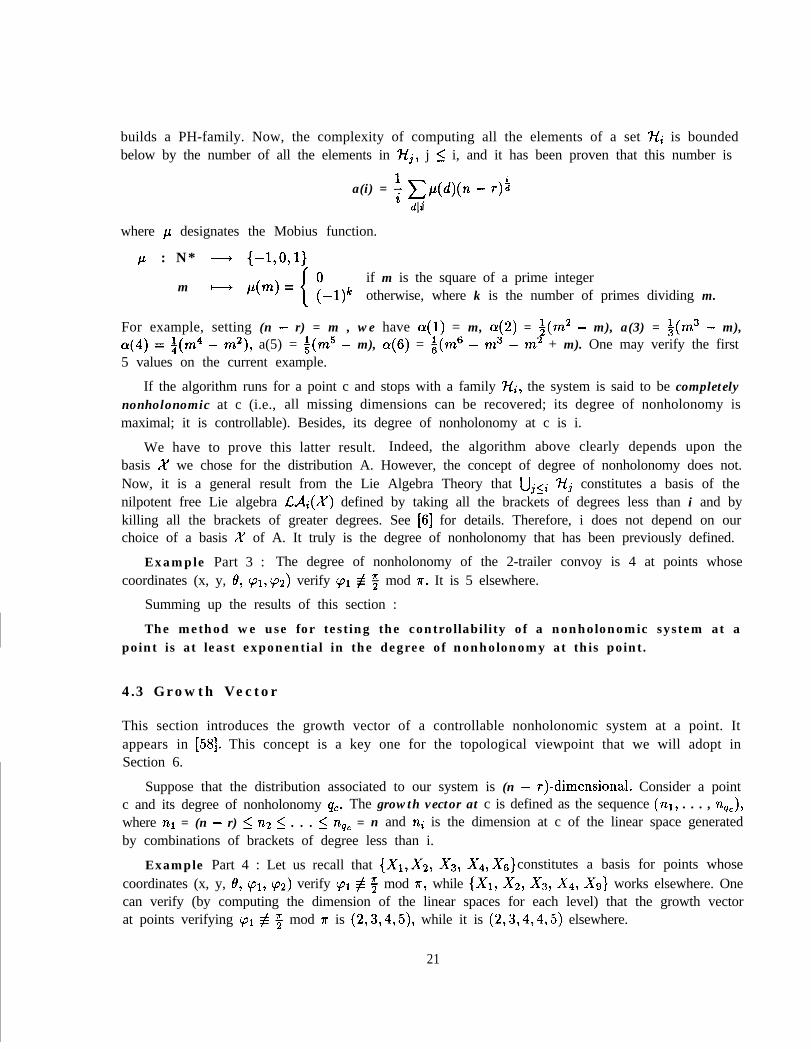
builds a PH-family. Now, the complexity of computing all the elements of a set ti; is boundedbelow by the number of all the elements in 3-1i, j 5 i, and it has been proven that this number is

a(i) = + gp(d)(n - r);i

where p designates the Mobius function.

P : N* - I-1,OJl

mif m is the square of a prime integerotherwise, where k is the number of primes dividing m.

For example, setting (n - r) = m , we have o(1) = m, a(2) = f(m2 - m), a(3) = i(m3 - m),o(4) = a(m4 - m2), a(5) = $(m5 - m), o(6) = i(m6 - m3 - m2 + m). One may verify the first5 values on the current example.

If the algorithm runs for a point c and stops with a family 3-t;, the system is said to be completelynonholonomic at c (i.e., all missing dimensions can be recovered; its degree of nonholonomy ismaximal; it is controllable). Besides, its degree of nonholonomy at c is i.

We have to prove this latter result. Indeed, the algorithm above clearly depends upon thebasis X we chose for the distribution A. However, the concept of degree of nonholonomy does not.Now, it is a general result from the Lie Algebra Theory that Uj<; tij constitutes a basis of thenilpotent free Lie algebra L&(X) defined by taking all the brackets of degrees less than i and bykilling all the brackets of greater degrees. See [6] for details. Therefore, i does not depend on ourchoice of a basis X of A. It truly is the degree of nonholonomy that has been previously defined.

Example Part 3 : The degree of nonholonomy of the 2-trailer convoy is 4 at points whosecoordinates (x, y, 6, ~1,92) verify cpr $ t mod 7r. It is 5 elsewhere.

Summing up the results of this section :

The method we use for testing the controllability of a nonholonomic system at apoint is at least exponential in the degree of nonholonomy at this point.

4.3 Growth Vector

This section introduces the growth vector of a controllable nonholonomic system at a point. Itappears in [58]. This concept is a key one for the topological viewpoint that we will adopt inSection 6.

Suppose that the distribution associated to our system is (n - r)-dimensional. Consider a pointc and its degree of nonholonomy qC. The growth vector at c is defined as the sequence (nl, . . . , nq,),where n1 = (n - r) 5 n2 5 . . . 5 nq, = n and n; is the dimension at c of the linear space generatedby combinations of brackets of degree less than i.

Example Part 4 : Let us recall that {X1,X2, X3, X4,X6 constitutes a basis for points whose}coordinates (x, y, 8, (~1, (~2) verify cpl + g mod 7r, while {Xi, X2, X3, X4, X9) works elsewhere. Onecan verify (by computing the dimension of the linear spaces for each level) that the growth vectorat points verifying 91 $ f mod r is (2,3,4,5), while it is (2,3,4,4,5) elsewhere.

21

4.4 Singularities and Regular Systems

All the above tools work only locally. For instance, we have just seen that the growth vector is notthe same everywhere in the manifold. The global viewpoint is not easy to reach. A first step is tostudy what happens in a neighborhood of a point.

A filtration {Ai} is regular at a point c if the growth vector is constant in a neighborhood ofc [58] [57]. This means that all the ranks of A;(.) are constant in the neighborhood. Otherwise,the filtration is singulcrr and the corresponding point is a singularity. Most of the problems weencounter when we try to define growth vectors and degrees of nonholonomy derive from thepresence of singularities. By extension, we will say that a system is regular if the correspondingfiltration is regular everywhere.

Example Part 5 : The 3 body system is not regular; more precisely the corresponding filtrationis regular at points verifying 91 + 5 mod ?r . It is singular at the remaining points. Remark thatthe growth vector is strictly increasing for regular points.

For regular systems, the degree of nonholonomy is a constant. It can also be shown (see [51])that the growth vector is strictly increasing, so the procedure we designed always stops in thatparticular case.

4.5 Well-Controllability

At this stage of the presentation, let us return to the planning problem. This section introduces theconcept of well-controllability. As the regularity concept, it deals with the existence of singularities,but this is a more global one.

As we have seen in Section 2, a general idea for devising a nonholonomic motion planner forcontrollable systems is to define a procedure that searchs for an admissible collision-free path,taking any collision-free path as a seed for the search2’.

Very recently Lafferiere and Sussmann proved that this principle is a general one. A collision-free path is first computed without taking the nonholonomic constraints into account. Lafferiereand Sussman’s method [55] ( see Section 6.3 for more details) roughly consists of expressing thefirst holonomic path into some “local coordinate system” (a precise definition will be given inSection 6.1); from these coordinates, because the system is controllable, the authors show that itis possible to explicitely define an admissible control (and then an admissible path) that locallysteers the system from a given point (on the first path) to any other on the first path inside a givenneighborhood. Because the planner has to work a priori everywhere, one has to define a procedurethat guarantees to find a local coordinate system everywhere. The existence of such a coordinatesystem is a technical point essential for the method. It is solved by considering an extended systemassociated with the original one; this new system is obtained by adding virtual controls working onvector fields defined from a PH-family of the original system. Since the nonholonomic distribution A

is (n - k)-dimensional, it seems a priori that k additional controls would suffice to make the systemholonomic. In fact, in order to avoid singularities (understood as points where the transformation

20[28] pinpointed this method for the car-like robot, while [32] p resents a planner using this principle for this case.

22

matrix would be non invertible), one has generally to add more controls. Lafferriere and Sussmannnote also that additional controls make easier the choice of a transformation matrix with a goodcondition number.

Let us illustrate this point using our example.

Example Part 6 : Recalling Example Part 2, a local coordinate system defined from {Xl, X2,x3, x4, x6} will encounter singularities. Following Lafferiere and Sussmann’s method, a possibleextended control system is defined by {Xl, X2, X3, X4, X6, .X9}; in the process, four controls areadded to the original ones. The previous results show that it is everywhere possible to choose inthis family a basis that spans R5.

Now, consider the following family :

UO = x1 vo = x2

J5 = [Xl 7 x21 Ul = cos CplXl + sin cpr Yr VI = sin (~1x1 - cos cplY1yz = [hvl] U2 = cos (p2Ul + sin cp2Y2 V2 = sin (p2Ul - cos (p2Y2y3 = [U2, v21

It is easy to check (see Appendix 3 for the general case) that the determinant of {‘I/o, VI, V2, U2, Y3)is equal to 1. Therefore { Vo, VI, V2, U2, Y3) spans R5 everywhere21. According to the previouscomments, we can define a minimal extended system that never meets with any singularity. More-over, the transformation matrix has a good condition number. We introduce the concept of awell-controllable system.

Definition 1 : An n-dimensional nonholonomic system defined by a distribution A is well-controllable, if there exists a basis of n vectors fields in the Control Lie Algebra LA(A) such thatthe determinant of the basis is constant.

Obviously well-controllability implies controllability. The converse does not hold. Indeed, as wementionned in Section 4.1, a system can be controllable while the local degrees of nonholonomy areunbounded. This means that the filtration {A;} stabilizes locally, but not globally. In this case, itis impossible to define a basis verifying the conditions of our definition.

The well-controllability concept is a global one and it is related to the planning problem. In-deed, for well-controllable systems, the same “local” coordinate system can work everywhere. Thissimplifies Lafferiere and Sussmann’s planning method. But, though we have a general procedure fortesting controllability, we have no general procedure for testing well-controllability. For instance,there is no obvious argument leading to reducing the search of a good basis to a small family, likea P H-Hall family.

Definition 2 : Let f? be a basis of the control Lie Algebra verifying the conditions of Defini-tion 1. The degree of well-controllability of the system is the maximum degree of all the elementsof a.

Remark : If the system is well-controllable, it is obvious that the global degree of nonholonomyis finite.

21Be careful * the degree of Ys equals 8, when it is viewed as a polynomial function with indeterminates XI and.X2 in Cd({Xl,&}).

23

Example Part 7 : The 2-trailer convoy is a well-controllable nonholonomic system. Its degreeof nonholonomy is 5, while its degree of well-controllability is at most 8.

4 .6 Geometric Models and Singularities : some Examples

Singularities typically come from the geometry of the system, though in some cases a bad choice ofbasis might create artificial singularities. Let us illustrate this point with three examples.

Consider once again the case of the l-trailer convoy. It appears (see Appendix 2) that this is aregular, well-controllable system of degree 3; its growth vector is (2,3,4) everywhere. Now considerthe same convoy, but with another hooking system. Instead of hooking the trailer exactly at themiddle of the rear wheels, we hook it to a point behind the rear axle (see Figure 2)22. Solving theequations yields the basis:

If we consider this basis only, we find a growth vector of (2,3,4) at points verifying sin cp # 0.The points verifying sin cp = 0 seem to constitute a singularity. But, checking our provisional basis,we find that the vector fields are collinear at these points, though the distribution is regular atthese points too. It is just awkward to find two vector fields which stay independent everywhere.For the record, any vector field of the form

is a valid vector field. With some ingenuity, for any value of a and u’, it is possible to obtain aglobal basis.

Now let us pinpoint a stranger case. We have seen that the 3-body convoy we study is con-trollable with degree 5 . Appendix 2 shows that the 2-body convoy is controllable with degree 3.The l-body convoy (i.e., the unicycle) is controllable with degree 2. Because of the singularity wementioned, there is no 4th degree. What is the fundamental difference between one trailer and twotrailers ? Furthermore, we prove in Section 5 that a n-body convoy is well-controllable and thatits nonholonomy degree is at most 2”. What is its precise nonholonomy degree ? What kind ofsingularities do we stumble upon ?

Finally, our third example doesn’t model any robotics systems whatsoever23 . Rather, it triesto capture the flavor of problems encountered in practice without any tedious computations: for

22[31] gives a constructive proof of controllability for this system.23This example was suggested by Marc Espie.

24

Figure 2: Another l-trailer car system

instance, the example of the 2-trailer system is quite similar to this one. Let us work in Euclideanspace (x, y, 2). Choose an integer n and consider the following vector fields :

and the distribution they engender.computing

Computing the associated filtration obviously sums up to

Now, this system is regular almost everywhere but not everywhere : the point (0, 0,O) is a majorinconvenience. At that point, for any k less than n, the vector field Yk vanishes altogether, so thatthe growth vector at (O,O,O) is (2,2, . . . ,3), giving thus a generic case where the nonholonomydegree is arbitrarily high. Furthermore, using standard techniques (Partitions of Unity), it is easyto piece together a denumerable infinity of such singular patches, so that the resulting distributionhas an unbounded degree.

This is the typical case where our Algorithm will not terminate. A finer study of the problemwould be a tremendous help.

4.7 Nilpotent and Nilpotentizable Systems

We have seen that the controllability testing procedure does not necessarily terminate in the generalcase. Notwithstanding, consider the following special case.

25

Suppose that al.l the Lie brackets of degree greater than k vanish. In this case, the sequence Xistabilizes :

xl c & c --’ c ctfk = &t(x).

We can stop the procedure Controllability as soon as alI the Lie brackets of degree k or less aregenerated. If the procedure does not yield a basis, then the system is not controllable.

Such systems are called nilpotent of oder k (see [6] for a general definition of the concept inthe Lie Algebra framework).

Example Part 8 : In our example, we may verify (see Appendix 2) that [X2, [X2, Xr]] = -Xl.Set adx(Y) = [X,Y]. Then24: adx2 ““(Xi) = (-1)” X1. The system is not nilpotent.

In some cases, a non-nilpotent system can be transformed into a nilpotent one via a linearchange of controls called a feedback tnxnsformation. Quite logically, such systems are called feedbacknilpotentizable. [55] gives some examples of feedback nilpotentizations (e.g., the unicycle, a car-likesystem and a car-like system with a trailer). See also [18] for sufficient conditions for a system tobe nilpotentizable.

Conjecture : Nilpotent and nilpotentizable systems are well-controllable.

The study of this conjecture, currently in progress, should help the quest for a general test ofwell-controllability.

4.8 Triangular Systems

The concept of a triangular system is used by Murray and Sastry in [39]. A system is triangular ifit can be defined as :

k, = v

22 = f2(21)2'

i3 = f3(2172)~.

with xi E Rmi and Cm; = n.

.2P = fp(x1,. * .,xp)v

Because of the triangular form, there exists simple sinusoidal control that may be used forgenerating motions affecting the ith set of coordinates while leaving the previous sets of coordinatesunchanged. It is possible to use these sinusoidal controls for planning trajectories (see [39] fordetails).

Even if a system is not triangular, it may be possible to transform it into a triangular one byfeedback transformations. Recent work [37] shows that a regular nilpotent controllable system can

. be t riangularized.

24This example appears in [55] for the unicycle and the car-like robot, i.e., systems equivalent to our current systemwithout trailers (see Section 4).

26

Conjecture : Triangularizable systems are well-controllable.

The next section will mention as an apurte that the multibody car system we consider alongthis paper is triangularizable.

27

5 The Multibody Car System is Well-Controllable

Let us return now to the general case of our convoy with n trailers. We know a basis {Xa,Xb} ofthe distribution A of the system (see Section 3.2) and we want to prove the existence of a family offields in LA(A) that spans the full tangent space when applied anywhere. To solve this problem,the only difficulty is to find a good family. Moreover, a minimal family that works everywhere (cfthe concept of well-controllability) is highly desirable.

Since the number of trailers is not fixed, we have to compute the general form of the (n + 3)coordinates of the vector fields we use.

Recall the form of X, and Xb :

x, =

cos 9sin e

0- sin ‘pi

sin cpi - cos y1 sin 92

.i - 2

(sin vi-1 - cos (pi-1 sin cp;) n cos ‘pjj=l

n - 2(sin (Pn-i - COS (Pn-l sin $C&,) JJ COS Q9j

j=l

Xb =

0 '0110...0 ,

The vector fields of the basis are obtained through the use of the same combinations as in Section4.6 (Example Part 5).

We build iteratively three brackets of degree 2i from brackets of degree 2i-1 :

Step0 Yo = x, 20 = Xb1 Xl = [yo, 201 fi = cos ylY0 + sin ~1x1 21 = sin qrY0 - cos qiXi2 x2 = [K, &I y2 = cos 92Yl + sin q2X2 22 = sin 92Yr - cos (~2x2. . . .. . . ..i Xi zL [x-l, Zi-11 Y; lz COS CpiE;:-1 + sin CpiXi 2; i sin viY;:-r - COS CpiXi. . . .. . . .. . . .

The general form of the vector fields coordinates is given by a lemma (Lemma 1, in Appendix 3).It remains for us to choose n + 3 vector fields that constitute a basis of Rn+3.

Lemma 2 : For any point c, {Ze,Zi, 22, . . . , Zn,Yn,Xn+r} (c) spans R.n+3.

28

Proof : We just have to exhibit the following determinant :

0 /3 p /? . . . p cosa -sine0 p /? /? . . . p sin (Y coscy1 0 0 0 . . . 0 0 01 - 1 0 0 . . . 0 0 00 1 - 1 0 . . . 0 0 00 0 1 - 1 . . . 0 0 0

. . .. . .. . .0 0 0 0 1 - 1 0 0

nwhere a = (0 - C 9;) (we do not need to express /3). It appears clearly that this determinant

i=lequals (-1)“. Q.E.D.

Finally, since the determinant does not vanish anywhere, we can conclude :

Property : The multibody car systems defined in Section 3.3 are well-controllable, with degreeat most 2n+1.

. . . and the driver of our luggage carrier can play rambling through the airport in search of a parkingplace ! An estimate of the time he needs to park his vehicle is the subject of the following section.

Remark: We have seen that such a system is not nilpotent. Because of the presence ofsingularities, it is not regular either. Nonetheless, the form we obtained for the determinant clearlyshows that such a system is triangularizable.

29

6 The Complete Problem

In Section 2 we saw that the existence of an admissible collision-free trajectory for a controllablenonholonomic system is characterized by the existence of a collision-free trajectory for the associatedholonomic system. Planning a trajectory can thus be achieved through the following steps:

l using a geometric planner for finding a trajectory without taking into account nonholonomicconstraints25 , and then

l steering the system as close by as possible to this trajectory along an admissible trajectory.

Such a general strategy has been refined into two different approaches that we will examinein Sections 6.3 [55] and 6.4 [33]. The first one uses a constructive proof of local controllabilityfounded on fundamental tools of differential geometry introduced in the next section (Section 6.1).The second one uses an explicit form for canonical feasible trajectories (e.g., shortest trajectories).

Both approaches come up against the following key problem : how to guarantee that theadmissible trajectory lies as close to the steering trajectory as the obstacles require ? The topologicalnature of this question is discussed in Section 6.2.

6.1 From Vector Fields to Trajectories

In this subsection we will investigate the delicate problem of finding trajectories that are compatiblewith our nonholonomic constraints. We need some precise concepts of differential geometry, whichare thoroughly studied in [50] [57] [51] [52].

Let us first take the very simple example of an Euclidean plane. At any point, the tangent spaceis a two-dimensional Euclidean vector space, though one should not confuse the tangent space withthe manifold itself. Pictorially, just view the Euclidean plane as a table and the tangent space ata point as a sheet of paper glued to the table at this very precise point. Considering the tangentspace at another point just involves sliding the sheet and gluing it at the other point. One can thentake a distinguished system of coordinates in these tangent spaces, namely the constant vectors Xand Y. These vectors induce a system of coordinates on the manifold in a straightforward way.Starting from a given point (the origin), just move in the X direction for a given time, say a, thenin the Y direction for a time b. You have reached the point of Cartesian coordinates a and 13. Thereare some alternate ways to achieve that : you could have first followed Y for a time b, then Xfor a time a or, with self-assurance, have directly taken the direction of choice, the straight linealong aX + bY. We can deduce some interesting facts from these simple manipulations. First, eachof these procedures gives rise to a system of coordinates. That means that we have a one-to-onecorrespondence: every point is defined by its coordinates and reciprocally. That also means thatthe correspondence is smooth, two neighboring points have neighboring coordinates and the wholescheme is thoroughly unsurprising.

25Finding such a trajectory corresponds to the classical Piano Mover problem. This problem is decidable. From atheoretical point of view, general algorithms exist in the literature. Notwithstanding, at this time, there is no generalsoftware that runs efficiently in practice. This is due to the intrinsic combinatorial complexity of the problem.

30

We are now going to use the same scheme for our purposes. The main difference is that ourvector fields won’t be constant any longer, and won’t even need to be globally defined. We couldsay that, instead of dealing with a flat Euclidean space, we will now work in a skewed space, wherevector fields are allowed to behave horribly. But, nonetheless, the same constructions will worklocally and give rise to some systems of coordinates-these are no longer equivalent.

Choose a point p in our manifold and a vector field X defined around this point. There isexactly one trajectory r(t) starting at this point and following X. In a formal notation, it verifiesY(O) = P and w = x,(t).

One defines the exponential of X (denoted by eX) to be the point y(l). This gives a corre-spondence between the space of vector fields and a neighborhood of p. It is obvious that one hasetX = r(t), namely this definition doesn’t describe a peculiar point of a trajectory but, more ac-curately, links every point of the trajectory to a specific vector field. Let us translate our previousexample to this formalism. Following aX + bY for a given time (the unit time) simply means totake eaX+bY. Following X for a time a amounts to following aX for the unit time, that is takingeaX, and following Y for a time b is the same as taking e bY This is still a slightly different point of.view : instead of considering the exponential to define a specific point of a trajectory with regardto an origin point p, we understand it as describing a motion from a point to another on a giventrajectory. Thus, starting at the origin o, following aX for a given time, then bY leaves us at thepoint ebY . eaX . o Therefore the exponential of a vector field X appears as an operation on themanifold, meaning “slide from the given point along the vector field X for unit time.”

In that setting, everything works nearly as smoothly as in the Euclidean case, at least locally.The main difference is that, whenever [X, Y] # 0, following directly aX + bY or following firstaX then bY are no longer equivalent. Intuitively, [X, Y] measures the variation of Y along thetrajectories of X; in other words, the field Y we follow in aX + bY has not the same value as thefield Y we follow after having followed aX (indeed Y is not evaluated at the same points in bothcases). The main result is the following :

Assume that X1, . . .,X, are vector fields defined in a neighborhood U of a point p suchthat at each point of U, X1, . . . , X, constitutes a basis of the tangent space. Then there is asmaller neighborhood V of p on which the correspondences (al, . . . , a,) I-+ ealX1+‘*‘+anXn . p and(%*.., a,) +.+ eanxn . . . @1X1 l p are two coordinate systems, called the first and the second normalcoordinate system associated to {Xi,. . . , X,}.

The Campbell-Haussdorf-Baker-Dynkin formula states precisely the difference between the twosystems :

For a sufficiently small t, one has : etX . etY = e~X+tY-~t2[X~Y]+t2E(t), where c(t> -+ 0 whent + 0.

Actually, the whole Campbell-Haussdorf-Baker-Dynkin formula as proved in [57] gives an ex-plicit form for the c function. More precisely, E yields a formal series whose coefficients lie inLA({X, Y}) : the coefficient of t” is a combination of brackets of degree k. In the case of a nilpotentsystem of order k, since brackets of degrees greater than k vanish, the Campbell-Haussdorf-Baker-Dynkin gives an exact development of the exponential. This property is used in the Lafferiere andSussmann’s planner presented below.

31

Roughly speaking, the Campbell-Haussdorf-Baker-Dynkin formula tells us how a nonholonomicsystem can reach any point in a neighborhood of a starting point. This formula is the hard coreof the local controllability concept. It yields a method for explicitly computing trajectories in aneighborhood of a point.

Now we take a closer look at the problem of obstacle avoidance.

6 .2 Obstacle Avoidance : the Topological Question

6.2.1 What Kinds of Topologies ? An Informal Statement

Let us come back to the sources. Motion planning in Robotics deals with obstacle avoidance. Realobstacles get transformed into “obstacles” in the configuration space. The Hausdorff metric26 onthe bodies, which are closed compact subsets, in the environment (that is to say, 3-dimensionalEuclidean space) induces a metric in the configuration space. Therefore, the reference open setsin the configuration space are the open sets in the topology induced by the Hausdorff metric inEuclidean space. This is the topology needed for solving placement problems27. A path appearsas a continuous function from a closed interval of R to the configuration space equipped with thistopology.

In some cases, the very act of considering motions can lead to a finer topology. If we introducethe distance induced by the best trajectory(ies) between two points with respect to a given cost(length, energy, time taken, etc), differential considerations take the scene. Consider the case ofenergy for instance. For holonomic systems, since every smooth path in the configuration space isan admissible trajectory, this cost induces a natural Riemannian distance. In that case, the inducedtopology remains the same.

For general nonholonomic systems, there may exists points at an infinite distance of each other.The non-holonomic constraints partition the configuration space into disconnected submanifolds,and the resulting topology has little ressemblance to the natural one. However, for controllablenonholonomic systems, any two points can be joined by an admissible trajectory; considering thebest trajectory leads once again to a well-defined metric. This is the origin of sub-Riemanniangeometry. Recent contributions show that Riemannian and sub-Riemannian metrics are equivalent.Therefore both topologies are the same. The next section state these results more thoroughly.

6.2.2 Of Sub-Riemannian Metrics, Shortest Paths and Geodesics

This section makes use of the ideas given in [58] for the case of regular systems. Consider acontrollable nonholonomic system (i.e., a completely nonholonomic one) defined on a n-dimensional

26A Hausdorff metric can be defined for any space equipped with a distance d. It yields the following topology oncompact subsets :

&(A, B) = ~~~~Ex(w+,EY d(z, Y)).

27See the problem of cloth orGeometry.

leather cutting as an example of such a problem in the context of Computational

32

manifold CM (for “Configuration Manifold”) by a distribution A. The nonholonomic metric28[58]is defined by

’&c,c’) = i n fJ-ES(c,c’) 0

(W, +w) 3 dt,

whereS(c, c’) = (7 1 [0, l] + CM, ~(0) = c, y(l) = c’, 9 E A} .

In that setting, geodesics are admissible trajectories that locally solve the variational problem.

The proof of the equivalence of the Riemannian and the sub-Riemannian metric resides in atwo-sided estimate of the size of sub-Riemannian balls. Denote by B,(c) the sub-Riemannian c-ball,i.e., the set of points reachable from c by an admissible trajectory of length less than 6’. Assumethat the system is regularr at c (see Section 4.8). Let {c;} be the local coordinate system definedin Section 6.1. Now consider the parallelepiped P,,c(c) = {c’ E CM 1 Ica( c’)I 5 odi)) where cp( i)is derived from the growth vector {n 1, . . . , npc} of A at c as cp(;) = j for nj-1 < i < nj2’. A twosided-estimate of B,(c) is given by the parallelepiped theorem [5813’ : there are positive constantscyi, ~2, ~0, such that for E < ~0,

P,l,&) c B,(c) c KY2,E(C).

Therefore, for regular systems, Riemannian and sub-Riemannian topologies are the same.

Remark : The parallelepiped theorem holds only at regular points. There are some technicalproblems at singular points (e.g., as at the singularities appearing in the 2-body system). It seemspossible to extend the proofs (using a local coordinate system, i.e., valid everywhere in a neighbor-hood of a regular point) to well-controllable systems by using a local coordinate system holding forsingular points as well as for regular points (such a system exists by definition). Nevertheless, asalways with singularities, some care will have to be taken.

Strange phenomena appear in this sub-Riemannian geometry framework. We know that, ingeneral, if shortest paths are geodesics, geodesics are not necessarily shortest paths-indeed, theyonly minimize length locally. One of the main features of Riemannian geometry is that, locally,geodesics are shortest paths. Consider the e-ball B,(c) ba ove, and S,(c) its boundary sphere. InRiemannian geometry, for E sufficiently small, the sphere S, is in one to one correspondence withthe ends of geodesics of length c (the so-called wave front). No similar property does hold fornonholonomic systems. [58] holds two drawings illustrating the strange relationship between thespheres and the wave fronts in the Heisenberg group case.

28This metric is also known as a singular [7], a Carnot-Carutheodory [36], or a sub-Riemannian [5l] metric.2gExample Part 9 : For the Z-trailer convoy at c = (O,O, O,O, 0), the growth vector is (2,3,4,5) (see Example Part

4). Therefore :

3o Bibliographic note : the proof of this theorem does not appear in [58]. A proof using different terminologyappears in [51].

33

Another strange phenomenon can be illustrated by the study of the car-like system31. In thisparticular case, the shortest paths have an explicit form (see the following section). Figure 3 is arendering of one of the corresponding spheres. Just notice that this sphere is not smooth and lookat the planes cutting the smooth part.

6.2.3 Geodesics and Shortest Paths : Elementary Computational Aspects

The classical way for computing geodesics is to use the maximum principle of Pontryagin [43].This is a powerful tool from classical Optimal Control Theory, which provides necessary conditionsfor the existence of an optimal control. The bang-bang principle is its direct consequence [l].Under some hypotheses, this principle gives the form of the optimal controls, if they exist. It hasbeen applied in [19] for Hilare-like robots (see Section 3.3.2) : in this case, geodesics are piecewiseclothoids or anticlothoids. Using the same ideas, we may verify that the geodesics for car-like robots(see Section 3.3.3) are piecewise arcs of circle or straight lines.

How to compute shortest paths is a much more difficult problem, even when an explicit formfor the geodesics (local shortest paths) is known. The problem is basically a combinatorial one :how to piece smooth geodesic parts together in order to produce a shortest path ? As far as theauthor knows, this question has only been answered for the car-like robot by Reeds and Shepp[44]. They extend the work of Dubins on the form of smooth shortest paths [14] and they establishprecisely which combinations of arcs of circle and straight line segments can produce shortest paths.Since the number of used combinations is finite, this gives birth to an efficient method to computeshortest paths.

6.3 A Planner Using Philipp Hall Coordinate Systems

This section is only a sketch of the general approach developed by Lafferiere and Sussmann in[55]. First, they study nilpotent and nilpotentizable systems. For such systems we have seenthat it is possible to compute a basis a of the Control Lie Algebra LA(A) from a Philipp Hallfamily. Their method assumes that a holonomic trajectory y is given. If we express locally thistrajectory on B, i.e., if we write the tangent vector T(t) as a linear combination of vectors in a(y(t)),the resulting coefficients define a control that steers the holonomic system along y. Using theCampbell-Haussdorf-Baker-Dynkin formula, it is then possible to compute an admissible controlu for the nonholonomic system that steers the system exactly to the goal (indeed, since all thebrackets vanish after a given level k, the Campbell-Haussdorf-Baker-Dynkin formula gives an exactdevelopment of the exponential on brackets of degree less than k, so the synthetized trajectory endsexactly at the same point.

For a general system, Lafferiere and Sussmann reason as if the system were nilpotent of order k.In this case, the synthetized trajectory deviates from the goal. Nevertheless, thanks to a topologicalproperty, this basic method is used in an iterated algorithm that produces a trajectory ending asclose to the goal as wanted.

311f we allow further inequalityto the sub-Riemannian geometry

constraints on the controls (see Remark in Section 3.3.3), [5] shows how to relateframework.

34

In both cases, the nonholonomic trajectory is a local approximation of y. In the presence ofobstacles, the “gap” due to the approximation has to be estimated in order to avoid the obstacles.This point is not clearly mentioned in the preliminary version of [55]. In fact, their algorithm canbe used as is by performing a recursive subdivision on the holonomic trajectory until all endpointscan be linked by collision-free trajectories synthetized by their algorithm above (this idea is alsoused in the second planner described below). It also seems that the parallelepiped theorem couldbe used to prove that the subdivision procedure always stops.

Remark : Lafferiere and Sussmann’s strategy can be extended to well-controllable systems byreplacing the Philip Hall local coordinate system by another one built from any basis workingeverywhere. This extension is currently under study.

6 .4 A Planner Using Shortest Paths

The planner developed by Jacobs and Laumond [33] uses a shortest paths approach. The threesteps of the algorithm are as follows :

l Plan a trajectory y for the corresponding holonomic system. If one does not exist, then nofeasible trajectory exists.

l Subdivide y until all endpoints can be linked by a minimal length collision-free feasible tra-jectory.

l Run through an “optimization” routine to reduce the length of the trajectory.

The convergence of the algorithm is a consequence of the parallelepiped theorem. Indeed, considera point c on y and NC a neighborhood of c included in the collision-free configuration space. Theparallelepiped theorem guarantees that there is a neighborhood NL of c, such that for each pointc’ E n/l the shortest trajectory between c and c’ lies in NC. Therefore since y can be covered by afinite number of such neighborhoods NC, the subdivision procedure will stop.

This planner has been totally implemented in an exact version for the special case of a polyg-onal car-like robot. This means we had to implement a geometric planner for computing an exactrepresentation of the collision-free configuration space. To do this, we used Avnaim and Boisson-nat’s algorithm [2]. We a so implemented a procedure for computing the shortest trajectories in1the absence of obstacles based upon Reeds and Shepp’s work. Finally, we designed a fast collisionchecking procedure. Figure 4, an excerpt from [33], hs ows how the algorithm responds to the clas-sical example of the parking problem. The three drawings give the trajectories produced by thethree steps of the algorithm.

An advantage of such a strategy is that it optimizes locally the trajectory (in terms of thetrajectory length). Indeed, the third step finds a quasi-optimal solution. Notice that finding theoptimal one is a problem known to be very difficult, and computationally very complex.

The main drawback of this general strategy is that we need to compute the shortest paths (seeSection 6.3.3). We are working on the Hilare-like system : at this time we know an explicit formfor the geodesics [19], but not for the shortest paths.

35

Notwithstanding, using general mathematical techniques for proofs of controllability and com-plexity analysis, we have laid a theoretical basis for a study of systems of greater complexity.Essentially, the method consists in establishing a catalogue of canonical trajectories having thenecessary topological properties, then in using them together with the subdivision motion planningtechnique. Clearly, the main question is : how to compute a sufficient set of canonical trajectories ?In the general case, the only way out seems to be the use of discretization techniques, but even inthis case, the theoretical background is required to find a discretization fine enough to solve theproblem. This latter aspect is currently under investigation.

6 . 5 Complexity of the Complete Problem

As discussed in Section 2, the decision part of the motion planning problem for controllable systemsis equivalent to the decision problem for the associated holonomic system. Hence the complexityof this problem is a polynomial function of the complexity of the environment (i.e., the numberof geometric primitives required to describe it), and the classical algorithms for the piano moversproblem can be applied.

Notwithstanding, the complexity of the complete problem (i.e., actually producing a trajectory)is more difficult to grasp. As a rule, any measure of complexity for this problem ought to be boundedfrom below by the complexity of the solution, which in turn ought to account for the number ofsingular points (cusps, loops,. . . ) it contains. Unfortunately, this number bears no relationship tothe customary description of the input data used for the piano movers problem. It actually dependson the inner size of the free space, measured in the sub-Riemannian setting adapted to the problem.

Before giving a formal definition of the complexity of a trajectory, as it appears in [5], we willfirst introduce the concept for a continuous function f: [a, b] ---) R. A good measure of what we callthe geometric complexity GC(f > fo such a function is the number of changes of variation. Moreprecisely, this complexity is defined as the quotient of the total variation of the function (see [45])by the amplitude of the function.

In the current context, our trajectories depend on the associated controls, which are continuousreal valued functions. Consequently, we define the complexity of a trajectory according to thecomplexity of the associated controls. If a trajectory y is defined by a control function u, itsgeometric complexity GC(y) is :

GC ((u, S)) denoting the geometric complexity of the continuous real valued function (u, 0, projec-tion of u along the axis supporting ,$ (see [5] for details).

This definition grasps every critical point of a trajectory, and so matches closely the outputcomplexity of any motion planner. In the current context, it also includes the number of maneuversas well as the number of loops and inflexion points.

This definition hints at some lower bounds for the complexity of complete motion planners. Forinstance [5] solves the case of the car-like robot. Given c and c’ two configurations in the same

36

connected component of configuration space, we proceed to define c. Choose an admissible pathbetween c and c’. At a point Q of that path, find the Euclidean diameter of the largest ball centeredat Q and wholly contained in the free configuration space. Take the infimum of this diameter forall points of the path. Then c is defined as the supremum of this quantity over all possible pathslinking c and c’.

Then the complexity of a trajectory of a car-like robot going between c and c’ is proportionalto O(r-2).

Roughly speaking, this means that, in the car parking problem (as shown in Figure 4), thenumber of necessary maneuvers asymptotically varies as the square of the inverse of the margin ofmaneuver.

The proof of this result is based upon the Campbell-Haussdorf-Baker-Dynkin development ofthe exponential. A detailed study of the general case exhibits very close relationship between thiscomplexity model and the degree of nonholonomy of the system. Everything depend upon the shapeof the parallelepipeds derived from the growth vectors (Section 6.2.2). A general proof, currentlyunder study, should lead to the following property :

Property : Given c, c’ two configurations in the same arcwise-connected component of theconfiguration space. Define c as the supremum, over all continuous paths from c to c’, of theinfimum, over all configurations q along that path, of the Euclidean diameter of the largest ballcentered at q and wholly contained in the free configuration space. The problem of finding thetrajectory for a regular controllable nonholonomic system of degree k between c and c’ is in O(c-“).

Conjecture : The problem is in O(c-“) for well-controllable systems whose well-controllabilitydegree equals k.

If our conjectures hold, this would mean that our luggage carrier driver would have todo 0 (,++“) maneuvers in order to park his machine in the neighborhood of regularpoints, and in O(E-~(“$~)) in the worst case . . .

37

Acknowledgments

In this study, I have benefited from an advanced preliminary collaboration with Paul Jacobs.I thank Marc Espie for rummaging with me through Stanford’s libraries, for a first writing ofSection 6.1, and for a critical reading of this report. I also thank Jean-Claude Latombe for severaluseful discussions on the controllability of a multibody system and for his invitation to stay in hislaboratory.

I wish also to thank Andre Bellaiche for introducing me to the sub-Riemannian Geometry,Richard Murray for pinpointing the reference [58], Shankar Sastry for discussions about triangularsystems, Philippe Soueres who has verified the computations of Appendix 3 and Michel Taix whohas implemented a main part of the planner for car-like robots and computed the shape of the sub-Riemannian ball shown in the paper. Finally, thanks to Georges Giralt who has felt the fecundityof the nonholonomic problem a few years ago, and presented it to me.

References

[l] M. Athans, and P.L. Falb. Optimal Control. McGraw-Hi& 1966.

[2] F. Avnaim, J.D. Boissonnat, and B. Faverjon. A practical exact motion planning algorithm forpolygonal objects amidst polygonal obstacles. In IEEE International Conference on Roboticsand Automation, Philadelphia (USA), pages 1656-1661, April 1988.

[3] J. Barraquand and J.C. Latombe. On non-holonomic mobile robots and optimal maneuvering.Revue d’lntelligence Artijkielle, 3(2), 1989.

[4] J. Barraquand and J.C. Latombe. Controllability of mobile robots with kinematic constraints.Technical Report STAN-CS-90-1317, Stanford University, June 1990.

[5] A. Bellaiche, J.P. Laumond and P. Jacobs Controllability of car-like robots and complexity ofthe motion planning problem with kinematic constraints. Int. Symp. on Intelligent Robotics,Bengalore, January 199 1.

[6] N. Bourbaki. Groupes et Alggbres de Lie : chapitres 2 et 3 CCLS Diffusion, Paris, 1972.

[7] R.W. Brockett. Control theory and singular Riemannian geometry. In New Directions inApplied Mathematics, Springer-Verlag, 1981.

[8] John Canny, Bruce Donald, John Reif, and Patrick Xavier. On the complexity of kinodynamicplanning. In 2gth Symposiurn on the Foundations of Computer Science, pages 306-316, WhitePlains, NY., October 1988.

[9] J. Canny, A. R ge e, and J. Reif. An exact algorithm for kinodynamic planning in the plane.6th ACM Symp. on Computational Geometry, Berkeley, 1990.

38

[lo] R. Chatila. Mobile Robot navigation: space modeling and decisional processes. In RoboticsResearch : The Third International Symposium, 0. Faugeras and G. Giralt (Eds), MIT Press,Cambridge, Massachusetts, 1986.

[ll] P. Calou, W. Choi, J.C. Latombe, C. Lepape and M. Yim. Indoor automation with manymobile robots. In IEEE IROS, 1989.

[12] W.L. Chow. Uber systeme von lenearen partiellen Differetialgleichungen ester ordung. Math.Ann., 117, pp 98-105, 1939.

[13] C. A. Desoer and Y. T. Wang. Linear-time-invariant servomechanism problem: A self-contained exposition. In C. T. Leondes, editor, Control and Dynamic Systems, pages 81-129.Academic, New York, 1980.

[14] L. E. Dubins. On curves of minimal length with a constraint on average curvature and withprescribed initial and terminal positions and tangents. American Journal of Mathematics,79:497-516, 1957.

[15] S.J. Fortune and G.T. Wilfong. Planning constrained motions. In ACM STOCS, pages 445-459, Chicago IL, May 1988.

[16] G. Giralt, R. Chatila, and M. Vaisset. An integrated navigation and motion control systemfor autonomous multisensory mobile robots. In Robotics Research : The First InternationaESymposium, M. Brady and R. P. Paul (Eds), MIT Press, Cambridge, Massachusetts, 1984.

[ 171 Hermann and Krener. Nonlinear controllability and observability. IEEE Transactions onAutomatic Control, 22(5), 1977.

[18] H. Hermes, A. Lundell, and D. Sullivan. Nilpotent bases for distributions and control systems.J. of Diflerential Equations, 55, 385-400, 1984.

[19] P. Jacobs, A. Rege, and J.P. Laumond. Non-holonomic motion planning for Hilare-like mobilerobots. In Int. Symp. on Intelligent Robotics, Bengalore, January 1991.

[20] Paul Jacobs. Minimal length curvature constrained paths in the presence of obstacles.LAAS/CNRS Report 90042, Laboratoire d’Automatique et d’Analyse des Systemes, Febru-ary 1990.

[21] Paul Jacobs and John Canny. Planning smooth paths for mobile robots. In Proceedings of the1989 International Conference on Robotics and Automation, pages 2-7. IEEE, May 11989.

[22] Paul Jacobs and John Canny. Robust motion planning for mobile robots. In Proceedings ofthe 1990 International Conference on Robotics and Automation, Cincinnati, Ohio, May 1990.IEEE.

[23] Paul Jacobs, Greg Heinzinger, John Canny, and Brad Paden. Planning guaranteed near-time-optimal trajectories for a manipulator in a cluttered workspace. Tech. Rep. RAMP 89-15,University of California, Berkeley, Engineering Systems Research Center, September 1989.

39

[24] K. Kedem and M. Sharir. An efficient motion-planning algorithm for a convex polygonal objectin two-dimensional polygonal space. Discrete and Computational Geometry, 5:43-75, 1990.

[25] Oussama Khatib. Real-time obstacle avoidance for manipulators and mobile robots. Interna-tional Journal of Robotics Research, 5(1):90-99, Spring 1986.

[26] B.H. Krogh and D. Feng. Dynamic generation of subgoals for autonomous mobile robots usinglocal feedback information. Transactions on Automatic Control, 34(5):483-493, May 1989.

[27] J.C Latombe. Robot Motion Planning. Kluwer Pub., to appear, 1990.

[28] J.P. Laumond. Feasible trajectories for mobile robots with kinematic and environment con-straints. In Intelligent Autonomous Systems, North Holland, 1987.

[29] J.P. Laumond. Finding collision-free smooth trajectories for a non-holonomic mobile robot. In10th International Joint Conference on Artificial Intelligence (IJCAI), Milan (Italy), 1987.

[30] J.P. Laumond, M. Taix, and P. Jacobs. A motion planner for car-like robots based on a mixedglobal/local approach. In IEEE IROS, July 1990.

[31] J.P. Laumond and T. Simeon. Motion planning for a two degrees of freedom mobile robotwith towing. LAAS/CNRS Report 89148 , Toulouse, April 1989.

[32] J.P. Laumond, T. Simeon, R. Chatila, and G. Giralt. Trajectory planning and motion controlfor mobile robots. In Geometry and Robotics, J.D. Boissonnat and J.P. Laumond (Eds), pages133-149. Lecture Notes in Computer Science, Vol 391, Springer Verlag, 1989.

[33] P. Jacobs, J.P. Laumond, M. Tayx, and R. Murray. Fast and exact trajectory planning for mo-bile robots and other systems with non-holonomic constraints. Technical Report LAAS/CNRS90318, September 1990.

[34] 2. Li and J. Canny. Motion of two rigid bodies with rolling constraint. IEEE Trans. onRobotics and Automation, 6, 1990.

[35] C. Lobry. Controlabilite des systkmes non lineaires. SIAM J. of Control, 8:573-605, 1979.

[36] J. Mitchell On Carnot-Caratheodory metrics. J. Diflerential Geometry, 21, pp 35-45, 1985.

[37] R. Montgomery, R.M. Murray, and S.S. Sastry. Triangulating differential equations on homo-geneous nilpotent Lie groups. (work in progress).

[38] R.M. Murray and S.S. Sastry. Mathematical Questions in Robotics, chapter MathematicalProblems in Grasping and Manipulation by Multifingered Robot Hands. American Mathe-matical Society, January 1990.

[39] R.M. Murray and S.S. Sastry. Steering nonholonomic systems using sinuoids. 29th C.D.C.,Honolulu, Dec. 1990

[40] Y. Nakamura and R. Mukherjee. Nonholonomic path planning of space robots via bi-directionalapproach. IEEE International Conference on Robotics and Automation, 1990.

40

[41] Colm 6’Dtinlaing. Motion planning with inertial constraints. Robotics Report 73, New YorkUniversity, July 1986.

[42] E. P p d p ula a o o OS and S. Dubowsky. On the nature of control algorithms for space manipulators.IEEE International Conference on Robotics and Automation, 1990.

[43] L. Pon r at y gin et al. The Mathematical Theory of Optimal Processes. L.S. Pontryagin SelectedWorks, Vol. 4, Gordon and Breach SC. Pub., 1986.

[44] J.A. Reeds and L.A. Shepp. Optimal paths for a car that goes both forwards and backwards.Pacific J. Mathematics, to appear.

[45] H.L. Royden. Real Analysis. The Macmillan Company, New York, 1968.

[46] E. Rimon and D.E. Koditschek. The construction of analytic diffeomorphisms for exact robotnavigation on star worlds. In Proceedings of the 1989 IEEE Int. Conference on Robotics andAutomation, pages 21-26, Scottsdale, May 1989.

[47] C. Samson and K. Ait-Abderrahim. Mobile Robot Control Part 1 : Feedback Control ofa Nonholonomic Wheeled Cart in Cartesian Space. Technical Report 1288, INRIA, SophiaAntipolis, 1990.

[48] M. Sharir. Algorithmic motion planning in robotics. Technical Report 392, Courant Institute,New-York University, 1988.

[49] M. Spivak. A Comprehensive Introduction to Differential Geometry, volume 1. Publish orPerish, Berkeley, CA, 1979.

[50] S. Sternberg Lectures on Diflerential Geometry Chelsea Pub., 1983.

[51] R.S. Strichartz. Sub-riemannian geometry. J. Diflerential Geometry, 24, 221-263, 19%.

[52] R.S. Strichartz. The Campbell-Baker-Hausdorff-Dynkin formula and solutions of differentialequations. J. of Functional Analysis, 72, 320-345, 1987.

[53] H.J. Sussmann and Jurdjevic. Controllability of nonlinear systems. J. of Diflerential Equations,12, 1972.

[54] H.J. Sussmann. Lie brackets, real analyticity and geometric control. In Diflerential GeometricControl Theory, Brockett, Millman, Sussmann Eds, Birkhauser, 1982.

[55] G. Lafferriere and H.J. Sussmann. Motion planning for controllable systems without drift : apreliminary report. Technical Report SYCON-90-04, Rutgers Univ., June 1990.

[56] P. Tournassoud. Motion planning for a mobile robot with a kinematic constraint. In Geometryand Robotics, J.D. Boissonnat and J.P. Laumond (Eds), pages 150-171. Lecture Notes inComputer Science, Vol 391, Springer Verlag, 1989.

[57] V.S. vara ara’an. Lie Groups, Lie Algebra, and their Representations, Springer-Verlag, 1984.d J

41

[58] A.M. Vershik and V.Ya. Gershkovich. Nonholonomic problems and the theory of distributions.Acta Applicandae Mathematicae, 12, pp 181-209, 1988.

[59] G.T. Wilfong. Motion planning for an autonomous vehicle. In IEEE Int. Conf. on Roboticsand Automation, 1988.

[60] C.K. Yap. Algorithmic and geometric aspects of Robotics, chapter Algorithmic motion plan-ning. J.T. Schwartz and C.K. Yap (eds), Lawrence Erlbaum Associates, London, 1987.

42

7 Appendix 1 : Related Work and Background

This section presents an overview of results recently obtained in constrained motion planning.They are complementary to those mentioned in the main paper, in the extent that they take acomputational point of view into account.

7.1 Car-like and Trailer-like Robots

[28] envisaged the controllability of a car-like robot. The main result is that the existence of acollision free trajectory for such a system is characterized by the existence of a connected componentin the free configuration space. The constructive proof of this result has led to the implementationof a planner [32]. This planner uses an approximate representation of the free configuration spacedecomposed into parallelepipeds.

The planner described in [3] uses a discretization of the phase space, the adjacency relationbetween two cells taking kinematic constraints into account. Collision tests are obtained from abitmap representation of the 2D environment. The search algorithm applies a best-first searchstrategy whose cost function is the number of maneuvers. The planner then produces paths witha minimal (for the discretized representation) number of maneuvers.

Notice the heuristic approach developed in [56] : the 2D environment is decomposed into aset of corridors in which a specific technique for planning smooth paths is applied. Finally [59]proposes an algorithm that produces a motion with the minimum number of turns for a set of lanesextracted from the environment.

The case of trailer-like robots was attacked by Laumond and Sirneon [31]; they establishedthe controllability of such systems by applying the Lie Algebra formalism briefly recalled in theintroduction. They also give a second constructive proof, but this one does not lead to an efficientalgorithm.

The Barraquand and Latombe planner cited above also applies to the case of a robot withtrailers. Their planner is thus the first to produce paths for such a system.

7.2 Smooth Paths

Planning smooth, maneuver-free, paths for a mobile robot appears to be a more difficult problemthan when we allow maneuvers. In fact, there is no comparable controllability result. It is indeedpossible that a path exists for a holonomic system, and yet no smooth path exists. The specificproblem was first addressed by Dubins [14], who gives the form of the shortest bounded curvaturepath in the absence of obstacles. The problem of obstacle avoidance appears more recently in [28].In [29], the environments consist of closed curves which are not necessarily polygons. Unfortunately,the method presented there is not guaranteed to find a path. In Fortune and Wilfong [15], a decisionalgorithm is given to decide if a path exists under given conditions. The algorithm is exact, butdoes not generate the path in question. This algorithm runs in exponential time and space. Thealgorithm in [al] is a provably-good approximate algorithm solving the problem. It depends on asimplification of the set of smooth trajectories to a sufficient subset of canonical trajectories.

43

7.3 Shortest Paths

The study of shortest paths for constrained systems began with the seminal work of Dubins [14],who found the form of minimal length smooth paths with bounded average curvature for thenonholonomic system we study in this work. He established his result in the case that there areno obstacles. The algorithm presented in [21] is a provably good approximate algorithm, whichdepends upon an extension of the results of Dubins to the case where there are obstacles in theenvironment. This extension has been presented in a rigorous manner in [20]. When there areobstacles, minimal-length smooth paths consist of paths of the forms given by Dubins, alternatingwith parts of the obstacle boundaries. Finally, the same proof holds for a polygonal robot moving ina polygonal environment. However, in this case the portions of the obstacle boundaries are replacedby logarithmic curves which we call generalized tractrices. These curves are those that maintaincontact between an obstacle edge and a robot vertex while satisfying nonholonomic kinematicconstraints [56]. A study is currently in progress to exploit this characterization of the minimal-length paths and develop a provably good algorithm finding smooth paths for a polygonal robot.

Recently Reeds and Shepp extended the work of Dubins to piecewise smooth paths with boundedcurvature, alas without obstacles [44]. That is, they allow maneuvers and cusps along the path.

Essentially they proceed to show that any path holding more than two cusps is reducible to apath with at most two cusps, no longer and possibly shorter. It is clear that between cusps, thepath must be of the form given by Dubins. Then they discard some of the allowable curves by theuse of a homotopy argument.

Because, in this paper, we have concentrated on the case in which maneuvers are allowed, wehave used these curves as the basis for the development of our algorithms.

7.4 Time-Optimal Paths

There has also been some work on planning time-optimal trajectories for systems with constrainedaccelerations. Fundamental work in trajectory planning with dynamic constraints is presentedin [41]. That paper introduces the idea of planning trajectories for a particle with constraintson its acceleration. Unfortunately, the analysis is restricted to the case of one dimension motion.In [B] the same problem is addressed in the multiple dimension case. That work discusses finding anear-time-optimal safe trajectory for a moving particle subject to uniform L, acceleration boundson each axis. Unfortunately, the constraints on accelerations which are allowed in such approaches,while they may be state-dependent [23], do not apply to the systems we study here. More recently,[9] presents the first exact algorithm for time-optimal kinodynamic motion planning in the two-dimensional case.

7.5 Control-Oriented Approaches

There are sound arguments for applying ideas from Control Theory to motion planning. Controltheoreticians have long been interested in finding controllers which would be robust to modelingerrors, would reject disturbances and cope with parameter fluctuations (for example, see [13]).

44

There is a small body of literature on the obstacle avoidance problem using some ideas from ControlTheory. Most of this work centers on the technique of potential fields introduced by Khatib [25].In such problems, a potential function is set up so that the system will travel to the goal state bymoving in the direction of the negative gradient. Obstacles are avoided by making them areas ofhigh potential. This work suffers from being a local method that can abort before reaching thedesired goal state. However, an advantage is that these techniques are inherently robust. Extensionshave been proposed by Rimon and Koditschek [46] in an attempt to use this approach for globalpath planning. Krogh and Feng [26] have also proposed a method of global planning in which thelocation of a subgoal is continuously changed to lead the system around local minima generated bya set of convex obstacles to the actual goal.

45

8 Appendix 2 : The 2- and 3-Body Car Systems

This appendix presents the listings in Mathematics of computations of the various vector fieldscorresponding to the examples of the 2- and 3-Body Systems respectively.

(** A definition for Jacobians and Lie derivatives*(>

Clear[Jac, Lie]

Jac [x,, vect,1 := Table[D[x[[i]], vect[[j]ll, <i, Length[x]),(j, Length[vectlH

Lie[x,, y,, vect,] := Jac[y, vect1.x - JacCx, vect1.y

(** The 2-body system*I

vect = (x, y, theta, phi)(* a "simple" lie function, that simplifies brackets along the way *)<<Trigonometry.mdie CL, y-1 := Map[TrigCanonical, ExpandAll[Lie[x, y, vect]]]

(* Phillip Hall Family Hl *)xl = (Cos[theta], Sin[theta], 0, - Sin[phi])x2 = (0, 0, 1, 1)

(* Phillip Hall Family H2 *(>x3 = slie[xl, x2](* Phillip Hall Family H3 *)x4 = slie[xl, x3]x5 = slie [x2, x31

This yields the following results:

X l = {cos(@,sin(8),0,- sin(v)}x2 = w4171~X 3 = {sin(e),- cos(I?),O,cos(cp>}X 4 = w40,l~

46

det(x1, x2, x3,x4) =

(** The 3-body system*I

1

vect = (x, y, theta, Phil, phi21

(* Phillip Hall Family Hl *(>xl = (Cos[theta], Sin[theta], 0, - Sin[phil], Sin[phil] - Cos[phil] Sin[phi2])x2 = (0, 0, 1, 1, 03(* Phillip Hall Family H2 *)x3 = slie[xl, x21(* Phillip Hall Family H3 *(>x4 = slie[xl, x3]x5 = slieCx2, x33(* Phillip Hall Family H4 *(>x6 = slie[xl, x4]x7 = slie[x2, x4]x8 = slie[x2, x5](* Phillip Hall Family H5 *>x9 = sliecxl, x6](* an actual controllability algorithm would stop here *>

x10 = slie[x2, x6]xl1 = slieCx2, x7]xl2 = slie[x2, x8]xl3 = slieCx3, x43xl4 = slieCx3, x53

In that case, we obtain the following vector fields.

xl =x2 =x3 =x4 =x5 =x6 =

x7 =x8 =

{Cos(Qsin(WJ- sin(cp&sin(pl)- cos(cpI)sin(cpa)}{o,o, 1, l,O}{sin(8), - C4%O,COS(cpl),- co&%) - sin(cpl)sin(Q)}04 070, 1, -1 - cos(cp2)){cos(Qsin(QO,- sin(cp&sin(cpl) - cos(cpI)sin(cpa)}{O,(), 0, CO+pl), -2 COS(cpl) - c0s(cp1) cos(cp2))UA 0, 0, (40){ - sin(O), cos(O), 0, - COS(d,cos(W) + sin(a) sin(w)}

47

x9 = {O,O,O, 1, -2 - ~COS(~I)~ COS(cp2) - cos(p2)sin(pl)2}x10 = UA 0, 0, - sin(w), 2 sin(y$ + cos(cp2) sin(cpl)}xl1 = o-Ao,o,o,o}x l 2 = {- COSW, - sin(e), 0, sin(w), - sin(cpl) + cos(cpl) sin(&)xl3 = t0, ho, Sin(W), -2 sin(w) - cos(cp2) sin(cpl)}xl4 = {o,o,o,--1,l t cos(p2))

det(x1, x2, x3, x4, x6) = - cos(‘p~)

det(x1, x2, x3, x4, x9) = -1 - cos(cp~)~ cos(v2)

48

9 Appendix 3 : Proof of the Lemma in Section 5.

Note X[x] the x-coordinate of the vector field X.

Lemma 1 : The general form of X;, x and 2; is :

xi [xl = sin(8 - zpj)j=l

Xi[Y] = - COS(0 - gpj)j=l

X;[8] = 0

Xi[cp,] = 0...

Xi[Cpi-l] = 0

Xi[$9i] = COS $9;

Xi[Cpi+l] = - COS Cpi - sin Cpi sin Cpi+lXi[Vi+2] = sin $9;[Sin pi+1 - COS Vi+1 Sin (pi+21

...k - 2

xi [Vk] = [sin $9k-l - COS 9k-l sin pk] sin pi n COS pjj=i+l

.

E[xl = COS(0 - 6 vj)j=l

K[Yl = sin(8 - 2 vj)j=l

lq8] = 0

~[[cpol = 0

Y;[Cpi-11 = 0Y;[Cpi] = 0

Y;[Cpi+l] = - s i n pi+1K[‘Pi+2] = [Sin pi+1 - COS pi+1 sin vi+21

..k - 2

k;: k’k] = [ S i n yk-1 -COS $9k-1 Sin pk] n COS vjj=i+l

...

zi [X]

Z;[Ylzi [fl]zi [%I

Z;[Cpi-1]

Z;[Cpi]zi[Vi+l]

Z;[Vi+Z]

zi[Vk] =

= - sin@ - 5 pj)j=l

= cos(e - 6 pj)j=l

= 0= 0

= 0= - 1= 1= 0

..

0

Proof : As in the special case n = 2 developed in Section 4.6, we can verify that the lemmaholds for i = 1 (to do this, simply add n - 2 trailers and check the coordinates from ‘p1 to cpn).

49

Assume now that the lemma holds for Xi-l, Yi-1 and Zi-1. we will just verify the x, Cpi and (Pkcoordinates of Xi = [Yi-1,Zi-1], other computations being similar.

First, Zi-1 yields only four non-null coordinates, of which two are constant :

Zi-l[X] = sin(B - ‘2 Yj) Z;-l[Cp;-1] = -1j=l

zi-1 [Y] = COS(6- *ff pj) zi-l[Cpi] = 1j=l

Moreover all the partial derivatives with respect to x and y vanish. Therefore :

Xi[X] = zi-1 [X] - zi-1 [ph]

d= -zi-l [Vi-l]GK-1 [X]

d= G cos(e - 2 $9j)

t- j=l

= sin@ - &j)j=l

Xi[Cpi] = 2 (x-1 k’h$--& zi-1 [pi] - zi-1 [vh] ah=l

Y&K-l [Vi]>

= -zi-1 [Pi] kY,-1 [Vi]i

d= --dVi

( - SiIlv;)

= COS $9;

xi[vk] = 2 (=&hl~zi-1 [vk] - zi-1 [ph] ah=l

&$i-1 bi’k]>

= -zi-1 [Vk]dTX-1 [%I

a

= -b(ki cos vj)[sin vk-1 - cos yk-1 sin yk]’ j=i

k - 2= sin pi( n cos vj)[sin pk-1 - cos yk-1 Sin yk]

j=i+l

Q.E.D.

50

Figure 3: A S;HII(\ IAl under three different points of view.51

Computation of Holonomic path: 4.150

Computation of feasible

Time for optimization : 3.782 s

Figure 4: ‘I‘he three steps of the algorithm.52