
Non-recovery of two spotted and spinner dolphin ... · ery in the eastern tropical Pacific Ocean...
21
MARINE ECOLOGY PROGRESS SERIES Mar Ecol Prog Ser Vol. 291: 1–21, 2005 Published April 28 INTRODUCTION The bycatch of dolphins by the purse-seine tuna fish- ery in the eastern tropical Pacific Ocean (ETP), also known as the ‘tuna–dolphin issue’ (Gerrodette 2002), has been the subject of considerable scientific study and management actions over the past 30 years. Purse- seine fishing for tuna in the ETP can be carried out in 3 ways, only one of which has significant bycatch of dol- phins; the other modes of fishing have bycatch of fishes, sharks and turtles, but rarely dolphins (Edwards & Perkins 1998, Hall 1998). The part of the fishery that affects dolphins utilizes the association of seabirds, dolphins and fishes to locate and catch schools of yel- lowfin tuna Thunnus albacares (Au & Pitman 1986, NRC 1992). The large bycatch of dolphins in the 1960s and early 1970s led to the decline of several stocks of pantropical spotted and spinner dolphins, Stenella attenuata and S. longirostris (Smith 1983, Wade 1993). The 1972 passage of the USA Marine Mammal Protec- tion Act and its subsequent amendments led, by 1980, to a 95% reduction of dolphin bycatch by USA fishing © Inter-Research 2005 · www.int-res.com * *Email: [email protected] **Order of authorship determined by flip of a coin FEATURE ARTICLE Non-recovery of two spotted and spinner dolphin populations in the eastern tropical Pacific Ocean Tim Gerrodette 1, * , **, Jaume Forcada 1, 2 1 NOAA Fisheries, Southwest Fisheries Science Center, 8604 La Jolla Shores Drive, La Jolla, California 92037, USA 2 Present address: British Antarctic Survey, Natural Environment Research Council, Madingley Road, Cambridge CB3 0ET, UK Spotted dolphins Stenella attenuata and tuna purse-seine net in the eastern tropical Pacific. Fishermen use the association of tunas, dolphins and seabirds to locate large yellowfin tuna Thunnus albacares. The dolphin bycatch, which earlier led to population declines, is now much lower, but the dolphin populations have not yet recovered ABSTRACT: Populations of northeastern offshore spotted dolphins Stenella attenuata attenuata and eastern spin- ner dolphins S. longirostris orientalis have been reduced because the dolphins are bycatch in the purse-seine fish- ery for yellowfin tuna in the eastern tropical Pacific Ocean (the ‘tuna–dolphin issue’). Abundance and trends of these dolphin stocks were assessed from 12 large-scale pelagic surveys carried out between 1979 and 2000. Esti- mates of abundance were based on a multivariate line- transect analysis, using covariates to model the detection process and group size. Current estimates of abundance are about 640 000 northeastern offshore spotted dolphins (CV = 0.17) and 450 000 eastern spinner dolphins (CV = 0.23). For the whole period from 1979 to 2000, annual estimates of abundance ranged from 494 000 to 954 000 for northeastern offshore spotted dolphins and from 271 000 to 734 000 for eastern spinner dolphins. Manage- ment actions by USA and international fishing agencies over 3 decades have successfully reduced dolphin by- catch by 2 orders of magnitude, yet neither stock is show- ing clear signs of recovery. Possible reasons include underreporting of dolphin bycatch, effects of chase and encirclement on dolphin survival and reproduction, long- term changes in the ecosystem, and effects of other spe- cies on spotted and spinner dolphin population dynamics. KEY WORDS: Bycatch · Tuna–dolphin issue · Abundance · Eastern tropical Pacific · Stenella attenuata · Stenella longirostris · Population recovery · Fishery interactions Resale or republication not permitted without written consent of the publisher
Transcript of Non-recovery of two spotted and spinner dolphin ... · ery in the eastern tropical Pacific Ocean...

MARINE ECOLOGY PROGRESS SERIESMar Ecol Prog Ser
Vol. 291: 1–21, 2005 Published April 28
INTRODUCTION
The bycatch of dolphins by the purse-seine tuna fish-ery in the eastern tropical Pacific Ocean (ETP), alsoknown as the ‘tuna–dolphin issue’ (Gerrodette 2002),has been the subject of considerable scientific study
and management actions over the past 30 years. Purse-seine fishing for tuna in the ETP can be carried out in 3ways, only one of which has significant bycatch of dol-phins; the other modes of fishing have bycatch offishes, sharks and turtles, but rarely dolphins (Edwards& Perkins 1998, Hall 1998). The part of the fishery thataffects dolphins utilizes the association of seabirds,dolphins and fishes to locate and catch schools of yel-lowfin tuna Thunnus albacares (Au & Pitman 1986,NRC 1992). The large bycatch of dolphins in the 1960sand early 1970s led to the decline of several stocks ofpantropical spotted and spinner dolphins, Stenellaattenuata and S. longirostris (Smith 1983, Wade 1993).The 1972 passage of the USA Marine Mammal Protec-tion Act and its subsequent amendments led, by 1980,to a 95% reduction of dolphin bycatch by USA fishing
© Inter-Research 2005 · www.int-res.com**Email: [email protected]**Order of authorship determined by flip of a coin
FEATURE ARTICLE
Non-recovery of two spotted and spinner dolphinpopulations in the eastern tropical Pacific Ocean
Tim Gerrodette1,*,**, Jaume Forcada1, 2
1NOAA Fisheries, Southwest Fisheries Science Center, 8604 La Jolla Shores Drive, La Jolla, California 92037, USA
2Present address: British Antarctic Survey, Natural Environment Research Council, Madingley Road, Cambridge CB3 0ET, UK
Spotted dolphins Stenella attenuata and tuna purse-seine netin the eastern tropical Pacific. Fishermen use the associationof tunas, dolphins and seabirds to locate large yellowfin tunaThunnus albacares. The dolphin bycatch, which earlier ledto population declines, is now much lower, but the dolphin
populations have not yet recovered
ABSTRACT: Populations of northeastern offshore spotteddolphins Stenella attenuata attenuata and eastern spin-ner dolphins S. longirostris orientalis have been reducedbecause the dolphins are bycatch in the purse-seine fish-ery for yellowfin tuna in the eastern tropical PacificOcean (the ‘tuna–dolphin issue’). Abundance and trendsof these dolphin stocks were assessed from 12 large-scalepelagic surveys carried out between 1979 and 2000. Esti-mates of abundance were based on a multivariate line-transect analysis, using covariates to model the detectionprocess and group size. Current estimates of abundanceare about 640 000 northeastern offshore spotted dolphins(CV = 0.17) and 450 000 eastern spinner dolphins (CV =0.23). For the whole period from 1979 to 2000, annualestimates of abundance ranged from 494 000 to 954 000for northeastern offshore spotted dolphins and from271 000 to 734 000 for eastern spinner dolphins. Manage-ment actions by USA and international fishing agenciesover 3 decades have successfully reduced dolphin by-catch by 2 orders of magnitude, yet neither stock is show-ing clear signs of recovery. Possible reasons includeunderreporting of dolphin bycatch, effects of chase andencirclement on dolphin survival and reproduction, long-term changes in the ecosystem, and effects of other spe-cies on spotted and spinner dolphin population dynamics.
KEY WORDS: Bycatch · Tuna–dolphin issue · Abundance· Eastern tropical Pacific · Stenella attenuata · Stenellalongirostris · Population recovery · Fishery interactions
Resale or republication not permitted without written consent of the publisher

Mar Ecol Prog Ser 291: 1–21, 2005
vessels, due to a combination of scientific studies,increased regulations, observers on fishing boats, gearinspections and reviews of captain performance(Gosliner 1999). Similar programs, which were volun-tary at first and later became formal agreements, wereinitiated in the 1980s and 1990s under the auspices ofthe Inter-American Tropical Tuna Commission to coverfishing vessels of the international fleet (Joseph 1994).During the 1990s the USA restricted the importationand sale of canned tuna caught by setting on dolphins.As a result of these combined actions, dolphin bycatchin the ETP has declined by 99% in the internationalfishing fleet, and has been eliminated by the USA fleet,which does not set on dolphins. The annual numberof dolphins reported killed by the purse-seine tunafishery is currently <0.1% of the population size foreach ETP dolphin stock (Bayliff 2004).
Estimates of dolphin abundance are used to setannual limits on the dolphin bycatch under an inter-national agreement to conserve dolphin populations(Hedley 2001). Abundance estimates are also used inpopulation models to assess the status of the dolphinstocks (Wade et al. 2002, Hoyle & Maunder 2004).The surveys from 1998 to 2000 were part of a largerresearch effort to determine whether the fishery ishaving a significant adverse impact on the dolphinpopulations (Reilly et al. 2005). The answer to thisquestion has biological and economic consequences,because if the fishery is not having a significantimpact, the USA may adopt a less restrictive definitionof ‘Dolphin-Safe’ tuna.1 Under current fishing prac-tices, this re-definition would allow more canned tuna,particularly yellowfin tuna caught by the large Mexi-can fleet, to be sold as Dolphin-Safe in the USA andother countries. On Dec. 31, 2002, the Secretary ofCommerce of the USA decided that the fishery is nothaving a significant adverse impact. However, thisdetermination was challenged in court and overturnedin August, 2004, on the basis that the decision was notbased on science.
To assess the results of management actions,research vessel surveys to estimate abundance of theaffected dolphin stocks have been carried out periodi-cally since the 1970s by the National Oceanic andAtmospheric Administration (NOAA Fisheries). Thelatest series of cruises were undertaken in 1998 to2000. Abundance estimates based on cruises from
1986 to 1990 have been published as annual estimatesfor dolphins (Wade & Gerrodette 1992) and as pooledestimates over the entire 5 yr period for all cetaceanspecies (Wade & Gerrodette 1993). These estimateswere based on conventional line-transect analysis(Buckland et al. 2001).
Recent advances in line-transect analysis permitmodeling the probability of detecting objects along thetrackline as a function of factors other than perpendic-ular distance alone (Ramsey et al. 1987, Marques &Buckland 2003, Forcada et al. 2004, Royle et al. 2004).In addition, improved estimates of distances from shipto sighting (Lerczak & Hobbs 1998, Kinzey & Gerro-dette 2001, 2003) and group size (Gerrodette et al.2002) are now available. In this study we used multi-variate methods to estimate the abundance of spottedand spinner dolphins most affected by the ETP tunafishery. The estimates were based on data collectedfrom 1998 to 2000, together with a reanalysis of datafrom past cruises dating back to 1979. The entire setof estimates was analyzed for temporal trends, sincerecovery of the populations is expected after fishery-related mortality has been reduced to a low level.
MATERIALS AND METHODS
Stocks and survey design. Dolphin species in theeastern tropical Pacific have been divided into stocksfor management purposes, using data on distribution,population dynamics, morphology and genetics (Dizonet al. 1994). Two stocks designated as depleted underthe USA Marine Mammal Protection Act, and there-fore of primary interest in designing the surveys, werethe northeastern offshore stock of pantropical spotteddolphins Stenella attenuata attenuata north of 5° Nand east of 120° W (Perrin et al. 1994), and the ETPendemic eastern subspecies of spinner dolphins S. lon-girostris orientalis (Perrin 1990). These stocks will bereferred to as NE offshore spotted (NEOS) and easternspinner (ES) dolphins, respectively. The stratificationof the 1998–2000 surveys (Fig. 1D) was based on thedistribution of these stocks. The core stratum includesthe entire range of NE offshore spotted dolphins bydefinition, and most of the range of eastern spinnerdolphins. The boundary of the outer stratum wasdrawn well beyond the known range of easternspinner dolphins to be certain to include the entirepopulation.
Stratification of the surveys from 1986 to 1990(Fig. 1C) was different, based on the understanding ofstock structure and distribution at that time (Holt et al.1987). In this analysis, the original 4 strata of this serieswere increased to 6 by subdividing the Inshore andMiddle strata to match the currently defined boundary
2
1Under US law, the definition of Dolphin-Safe tuna is tunacaught by methods that do not involve the intentional chaseand encirclement of dolphins. The proposed change in de-finition would allow tuna caught by chasing and encirclingdolphins to be labelled Dolphin-Safe as long as no dolphinswere killed or seriously injured on that particular set ofthe purse seine. In either case the fishing vessel must carryan observer to certify that the standard has been met

Gerrodette & Forcada: Non-recovery of Pacific dolphin populations 3
160°
W14
0°W
120°
W10
0°W
80°W
20°S0°
20°N
A.
1979
NE
OS
= N
E O
FFS
HO
RE
SP
OTT
ED
ES
= E
AS
TER
N S
PIN
NE
R
NE
OS
2
NE
OS
1
NE
OS
3E
S 2
ES
1
160°
W14
0°W
120°
W10
0°W
80°W
20°S
0°20°N
B.
1980
-198
3
NE
OFF
SH
OR
E S
PO
TTE
D
EA
STE
RN
SP
INN
ER
160°
W14
0°W
120°
W10
0°W
80°W
20°S0°
20°N
C.
1986
-199
0
WE
ST
MID
DLE
1
MID
DLE
2
SO
UTHIN
SH
OR
E 2
INS
HO
RE
1
160°
W14
0°W
120°
W10
0°W
80°W
20°S
0°20°N
D.
1998
-200
0
CO
RE
OU
TER
NO
RTH
CO
ASTA
L
SOUTH COASTAL
Fig
. 1.
Stu
dy
area
s in
th
e ea
ster
n t
rop
ical
Pac
ific
du
rin
g 4
mar
ine
mam
mal
su
rvey
per
iod
s b
etw
een
197
9 an
d 2
000.
Geo
gra
ph
ic a
reas
are
str
ata
of s
urv
ey e
ffor
t (c
f. F
ig. 2
an
d T
able
1)

Mar Ecol Prog Ser 291: 1–21, 2005
of NE offshore spotted dolphins at 5° N. In 1980, 1982and 1983, a single stratum was used for each stock(Fig. 1B), and the amount of transect effort within thesestrata was less than in other years. In 1979, effort wasconcentrated in a smaller ‘calibration’ area (Fig. 1A,areas NEOS 1 and ES 1).
The surveys were conducted with 4 vessels: RV‘David Starr Jordan’, ‘Townsend Cromwell’, ‘McArthur’and ‘Endeavor’, which are similar in length (52 to 57 m)and observer eye height (10.4 to 10.7 m). In 1979 and1980, the surveys were conducted in January toMarch. The 1982 cruise took place in May to Augustand the 1983 cruise in January to April. Surveys in1986 to 1990 and 1998 to 2000 were carried out fromlate July to early December. Time of year, however,should not be an important factor affecting abundanceestimates, because the surveyed areas were largeenough to include any seasonal movements of the dol-phin populations (Reilly 1990).
Pre-determined transect lines were random withineach stratum, with the constraint that spatial coveragebe as even as possible. Ships moved at night, andthe starting point of each day’s transect effort waswherever the ship happened to be at dawn along theoverall trackline. Further details of survey design andtracklines are discussed in Gerrodette & Forcada(2002, and references therein).
Field methods. Weather permitting, a visual searchfor cetaceans was conducted on the flying bridge dur-ing all daylight hours as the ship moved along thetrackline at a speed of 10 knots (18.5 km h–1). On eachship, 3 marine mammal observers stood watch at atime, 2 using pedestal-mounted 25× marine binocularsand 1 using hand-held 7× binoculars and the nakedeye. When marine mammals were sighted, observersmeasured the angle and distance to the animals. Thepedestals of the 25× binoculars were fitted withazimuth rings for measurement of horizontal anglesfrom the trackline to the animals. Vertical angles fromthe horizon to the animals were measured with reticlescales in the ocular lenses of the binoculars. Reticlevalues were converted to angular values (Kinzey &Gerrodette 2001) and to distance from the observer,based on height above the water (Gordon 1990,Lerczak & Hobbs 1998). Reticle measurements of dis-tance were checked against radar under a varietyof field conditions; a slight tendency to underestimatedistances beyond 4 km, primarily due to atmosphericrefraction of light, was corrected by regression (Kinzey& Gerrodette 2003). Perpendicular distance d of thesighting from the trackline was computed as d = r sin θ,where r was the radial distance to the sighting and θthe horizontal angle of the sighting from the trackline.In addition to angle and reticle, Beaufort sea state,visibility, sun angle, swell height, presence of birds
and other factors that might affect detection probabil-ity were recorded with each sighting.
A data entry program automatically recorded theposition of the ship with a GPS signal from the ship. Ifthe sighting was <5.6 km (3 n miles) from the trackline,the observer team went ‘off effort’ and directed theship to leave the trackline and to approach the animalssighted (closing mode survey). The observers identi-fied the sighting to species or subspecies and madegroup size estimates. Observers discussed distinguish-ing field characteristics in order to obtain the best pos-sible identification, but they estimated group sizes and,in the case of mixed-species schools, group composi-tion independently. After completing the sighting,search effort was resumed toward the next waypoint.Further details of data collection procedures are givenin Kinzey et al. (2000).
On cruises before 1998, the same basic data (posi-tions at beginning and end of searching effort, anglesand distances to sightings, and school sizes) werecollected, although methods of collecting the dataevolved over the years. For example, previous datawere recorded on paper rather than on a laptop com-puter, and ship positions were measured with Loran orSatNav before the GPS system was available. On the1979 and 1980 cruises, distance and angle from track-line were estimated by eye rather than with binocularreticles and angle rings.
School size. From 1987 to 2000, RV ‘David StarrJordan’ carried a helicopter equipped with medium-format, motion-compensated, military reconnaissancecameras. In suitable conditions of sea state, sun angleand school configuration, entire schools of dolphinswere photographed from the helicopter and the num-ber of dolphins was counted directly from the nega-tives (Gilpatrick 1993). However, aerial photographswere available for only a subset of schools seen fromRV ‘David Starr Jordan’ and none of the schools seenfrom the other ships. For most schools, school size wasestimated from the best, high and low estimates madeby each observer.
By comparing each observer’s estimates of thephotographed schools to the counts from the negatives,individual correction or ‘calibration’ coefficients for 52observers were estimated (Barlow et al. 1998, Ger-rodette et al. 2002). These coefficients were used toproduce a calibrated estimate of school size when anobserver’s original (‘best’) estimate of school size fellin the range of photographed schools for which s/hehad been calibrated. Calibration coefficients were notavailable for every observer, either because (1) theobserver worked prior to the start of the aerial calibra-tion program in 1987, or (2) the observer had ≤ 5 photo-graphed schools to estimate the regression coeffi-cients. For school size estimates made by uncalibrated
4

Gerrodette & Forcada: Non-recovery of Pacific dolphin populations
observers, or for schools which fell outside the range ofschool sizes for which an observer had been calibrated,we divided the observer’s best estimate by 0.860, themean ratio of best estimate to photo count for the52 calibrated observers (Gerrodette et al. 2002).
We combined the individual estimates made by eachobserver, adjusted as described above, to obtain asingle estimate of size for each school. Because thecalibration procedure was based on the logarithm ofthe estimates, the weighting and averaging was alsocarried out on the logarithms, using the inverse of thevariance of each observer’s estimates as weights. Thelogarithm of the final calibrated estimate of school sizes for each sighting was:
(1)
with variance
(2)
where n is the number of calibrated estimates C for theschool, wi = vi
–1�Σvi–1 and vi = var(ln Ci) is the residual
variance of the log-log regression of school size esti-mates on photo counts for the observer making the i thestimate.
Abundance estimation. Estimation of abundancewas based on distance sampling (Buckland et al. 2001).A multivariate extension of conventional line-transectanalysis (Marques & Buckland 2003, Forcada et al.2004; see Appendix 1) estimated abundance as:
(3)
where Aj is the area and Lj is the length of search effortin stratum j, ƒij(0,cij) is the estimated probability densityevaluated at zero perpendicular distance of the i thsighting in stratum j under conditions cij, and sij is theestimated group size of the i th sighting in stratum j (orsubgroup size of the species of interest in the caseof mixed-species schools). Estimation was based onsearch effort and sightings that occurred during on-effort periods, in conditions of Beaufort <6 and visi-bility >4 km. The vector of covariates cij included thecontinuous variables: group size, Beaufort sea stateand time of day; and the categorical variables: species,ship, stratum, sighting cue, whether the school wasa single- or mixed-species group, presence/absenceof glare on the trackline, and presence/absence ofseabirds. Sea state measured on the Beaufort scale wasactually a discrete variable, but the ordinal scale couldbe modeled satisfactorily as a continuous variable(Barlow et al. 2001). The continuous variable swellheight was also recorded on the 1998–2000 cruises. Alldolphin schools on or near the trackline were assumedto be detected, i.e. g (0) = 1.0.
We explored half-normal and hazard-rate models,each with variable numbers and types of covariates.Hazard-rate models gave highly variable estimates ofeffective strip width among years, and unpublishedanalyses suggested grounds for biased ƒij (0,cij) esti-mates using this model for the study data. For consis-tency we used only the half-normal model, with sight-ings truncated at 5.5 km. For each species or stock ineach year, covariates were tested singly and in addi-tive combination, and a set of best models was chosenon the basis of Akaike’s Information Criterion cor-rected for sample size (AICc) (Hurvich & Tsai 1989). Forcomputational efficiency, we retained as reasonablemodels all models with an AICc difference (ΔAIC) ≤2from the best model. Final estimates of ƒij (0,cij) utilizedmodel averaging, with the AICc scores as weightingfactors. The weight of the estimate from the j thmodel was exp(–0.5ΔAICj)�Σ jexp(–0.5ΔAICj) (Burn-ham & Anderson 1998).
Pooled components of the abundance estimates werecomputed to provide additional summary and diagnos-tic statistics. Pooled components ƒ(0), expected schoolsize , school encounter rate n/L, and percentage ofthe total abundance estimate due to the prorated abun-dance of unidentified sightings (see next section) werecalculated across all sightings i and strata j as:
(4)
(5)
(6)
(7)
for each stock and year, where, for stratum j, nj is thenumber of sightings, Nid,j is the estimated abundancebased on identified sightings, Nunid,j is the proratedabundance estimate based on unidentified sightings,and other terms are defined in Eq. (3).
Specific code in S was written to implement theanalysis. The S code included calls to FORTRAN rou-tines for the maximum likelihood optimization of thecovariate density models. These routines consisted ofmodifications of Buckland’s (1992) algorithm to fitmaximum-likelihoods of density functions using theNewton-Raphson method.
Unidentified sightings. Not all sightings could beidentified to stock with certainty. The number of sight-ings recorded as unidentified was first reduced byassigning sightings recorded as ‘probable’ to that iden-tified category. For the remaining unidentified sight-ings, we estimated abundance for the unidentifiedcategory and prorated abundance among appropriate
ƒ( ) ƒ ( , )
( ) ƒ ( ,
0 0
0
=
=
∑∑ ∑ij ijij
jj
ij
c n
E s c�iij ij
ijij ij
ij
jj
jj
s c
n L n L
) ˆ ƒ ( , )
/
%
∑∑ ∑∑
∑ ∑=
0
prro ˆ ( ˆ ˆ ), , ,= +∑ ∑100 N N Nunid jj
unid jj
id j
E s( )�
ˆ ƒ ( , ) ˆNA
Lc sj
jij ij ij
ij
= ∑∑ 20
var(ln ˆ) var(ln )s w C vi ii
n
ii
n
= = ⎛⎝=
−
=∑ ∑2
1
1
1⎜⎜
⎞⎠⎟
−1
ln ˆ lns w Ci ii
n
==
∑1
5

Mar Ecol Prog Ser 291: 1–21, 2005
stocks in proportion, by stratum, to the estimatedabundance from identified sightings of those stocksthat were included in the broader unidentified cate-gory. The general form of the proration was:
(8)
where Nij is the revised abundance estimate of stock iin stratum j, N*ij is the abundance of stock i in stratumj estimated from identified sightings of stock i, Nuj isthe abundance of the unidentified category estimatedfrom unidentified sightings in stratum j, and N*kj is theabundance estimate of stock k in stratum j for stocksother than i included in the unidentified sighting cate-gory. This proration made the assumption that all taxawithin the unidentified category were equally easy toidentify. While probably unrealistic, this assumptionwas the simplest in the absence of data on ease ofidentification.
We estimated abundance of 3 unidentified sightingcategories: unidentified spotted dolphins (prorated toNE offshore spotted, western/southern offshore spot-ted, and coastal spotted dolphins), unidentified spinnerdolphins (prorated to eastern spinner and whitebellyspinner dolphins), and unidentified dolphins (proratedamong several species including spotted and spinnerdolphins). For example, to prorate the abundancerepresented by sightings of unidentified dolphins, weestimated abundance of spotted, spinner, striped (S.coeruleoalba), common (Delphinus spp.), bottlenose(Tursiops truncatus), rough-toothed (Steno bredanen-sis) and Risso’s (Grampus griseus) dolphins in eachstratum, and distributed the abundance of unidentifieddolphins proportionally among them.
Precision. Precision of the abundance estimates andpooled abundance components was estimated by bal-anced nonparametric bootstrap (Davison & Hinkley1997). Within each stratum, a balanced bootstrap sam-ple was constructed by sampling transects (days oneffort) with replacement, so that all transects wereselected the same number of times in total. To includethe variability due to school size estimation and thecalibration procedure, for each school size estimate s inthe bootstrap sample, the logarithm of a new schoolsize was chosen from a normal distribution with meanln(s) and variance var[ln(s)], equal to the estimatedmean and variance of the sighting’s school size esti-mate obtained by calibration. For each bootstrap sam-ple, the full estimation procedure was carried out,including proration and model averaging. To includemodel selection uncertainty and to avoid overestimat-ing precision, multiple models were used in each boot-strap. Models for ƒij (0,cij) estimation were restricted tothe set of models with ΔAIC ≤ 2, based on the original
data, plus the univariate half-normal model. From 1000bootstrap estimates, the standard errors (SE), coeffi-cients of variation (CV) and bias corrected and acceler-ated (BCa) (Efron & Tibshirani 1993) 95% confidenceintervals of the estimates of total abundance andpooled abundance components were computed.
Trend estimation. To examine trends in the time-series, we fitted weighted linear and quadratic (2nd-order) models to the estimates of NE offshore spottedand eastern spinner dolphins, using the inverse ofthe variance of each point estimate as the weightingfactor. The statistical significance of each model wastested against the null hypothesis of no change in pop-ulation size with time, using a Type 1 error rate of α =0.05. The statistical power (1 – Type 2 error rate) ofdetecting a change in population size, given the actualnumber of estimates at the observed intervals and pre-cision, was evaluated for simple exponential growth,using a modified version of Trends, a program to esti-mate power for linear regression (Gerrodette 1987,1993). The power analysis assumed a 2-tailed test ofsignificance with α = 0.05, rates of population growthfrom 1 to 5% and the mean CV for NE offshore spotteddolphins. To provide visual summaries of the time-series, the estimates were smoothed with nonparamet-ric LOESS smoothers, using the same inverse-varianceweights.
RESULTS
Sightings and effort
Total transect effort was 42 000 km in 1998 with 3ships, and 30 000 km each in 1999 and 2000 with 2 ships(Table 1). During the 1986–1990 cruises, total search ef-fort ranged from about 24 000 to 30 000 km each year,while total effort in 1983 and earlier was from 8600 to16 100 within the strata shown in Fig. 1. Total effort forall years was 295 000 km, but the amount and distribu-tion varied among years (Fig. 2, Table 1).
The annual number of sightings (schools) of NE off-shore spotted dolphins ranged from 107 to 184 in 1998to 2000 (core and north coastal strata), from 60 to 88 in1986 to 1990 (Inshore 1 and Middle 1 strata) and from20 to 56 from 1979 to 1983 (Table 1, Fig. 2). The annualnumber of sightings of eastern spinner dolphin schoolsranged from 67 to 94 in 1998 to 2000, from 38 to 71 in1986 to 1990 and from 14 to 30 in 1979 to 1983. Bydesign, more effort was concentrated in the range ofNE offshore spotted and eastern spinner dolphins in1998 to 2000 compared to previous years (Table 1,Fig. 2). The number of sightings of these dolphin stockstherefore tended to be higher, particularly in 1998when 3 ships were used.
ˆ ˆ * ˆˆ *
ˆ * ˆ *N N N
N
N Nij ij uj
ij
ij kjk
= ++
⎛
⎝
⎜⎜
⎞
⎠
⎟⎟∑
6

Gerrodette & Forcada: Non-recovery of Pacific dolphin populations
In addition to the identified sightings in Table 1,there was a large number of unidentified dolphinsightings each year. An unidentified dolphinsighting could potentially be any of a number ofspecies, including spotted and spinner dolphins.Unidentified dolphin sightings were usually smallgroups of animals seen at large radial distancesfrom the ship that subsequently could not be relo-cated, or groups seen at >5.6 km from the track-line that were not approached for identification.Although the number of unidentified dolphinschools was large, the contribution of these sight-ings to total abundance was small (see ‘Abun-dance’ below) because many of the sightingswere beyond the truncation distance of 5.5 km,group size was small, and only a fraction of theestimated unidentified dolphin abundance wasprorated to the stocks of interest.
Model selection, detection function, andgroup size
Models including school size, sea state, sightingcue and other covariates were important in mod-eling the probability of detecting schools of spot-ted and spinner dolphins (Table 2). The numberof plausible models (ΔAIC ≤ 2) ranged from 1 to 5,with multiple models chosen in most years. A uni-variate model with perpendicular distance as theonly predictor was chosen as the best model inabout half the cases, but it was never the onlymodel chosen. The number of covariates selectedranged from 1 to 3, with group size being the mostfrequently selected covariate. In general, estima-tion of ƒij(0,cij) was based on sightings of a partic-ular stock (Table 1). However, if the number ofsightings of a single stock was not adequate (usu-ally a minimum of about 40), sightings of allstocks within species were combined for ƒij(0,cij)estimation. In 1980, 1982 and 1983, when theamount of survey effort and number of sightingswere small, we combined spotted and spinnersightings for ƒij(0,cij) estimation, because the spe-cies are similar in body and school size and,indeed, often occur together in the same school.Although different models were generallyselected (Table 2), the mean estimates of ƒ(0)were similar (Table 3).
The histograms of sighting frequency byperpendicular distance for spotted (Fig. 3) andspinner (Fig. 4) dolphins frequently showed aspike in the frequency of sightings near the track-line. As noted in ‘Materials and methods’, fittingthe probability density function to this spike with
7
Table 1. Size of study area for surveys of Stenella attenuata attenu-ata and S. longirostris orientalis, amount of survey effort and num-ber of sightings, by year and stratum. Sightings: number of identi-fied dolphin schools within 5.5 km perpendicular distance of thetrackline during periods of searching effort in conditions of Beaufort< 6 and visibility > 4 km. Strata are shown in Fig. 1. Distribution of
effort and sightings is shown in Fig. 2
Stratum Area Effort Sightings (no. of schools)(106 km2) (km) Offshore Eastern
spotted spinner
1979NEOS 1 2.302 8785 51 –NEOS 2 3.895 3758 5 –NEOS 3 0.371 62 0 –ES 1 2.398 9135 – 29ES 2 7.232 4397 – 1
1980NE offshore spotted 6.568 6103 36 –Eastern spinner 9.630 9965 – 14
1982NE offshore spotted 6.568 5631 20 –Eastern spinner 9.630 6575 – 15
1983NE offshore spotted 6.568 4347 24 –Eastern spinner 9.630 4209 – 14
1986Inshore 1 4.603 9077 59 42Inshore 2 1.400 2630 10 1Middle 1 2.000 3345 18 15Middle 2 1.810 4317 15 0West 5.218 3848 16 3South 4.539 3882 5 0
1987Inshore 1 4.603 8361 58 38Inshore 2 1.400 2934 2 0Middle 1 2.000 4327 21 14Middle 2 1.810 3655 23 0West 5.218 3823 15 2South 4.539 4492 12 0
1988Inshore 1 4.603 7336 49 31Inshore 2 1.400 2065 4 2Middle 1 2.000 3530 11 4Middle 2 1.810 2648 7 0West 5.218 3209 16 1South 4.539 5019 5 0
1989Inshore 1 4.603 9006 72 54Inshore 2 1.400 2719 7 0Middle 1 2.000 4303 16 14Middle 2 1.810 3597 16 2West 5.218 3659 15 1South 4.539 4788 7 0
1990Inshore 1 4.603 7321 60 29Inshore 2 1.400 2727 3 0Middle 1 2.000 4652 19 12Middle 2 1.810 4211 18 2West 5.218 5484 11 2South 4.539 6556 8 0
1998Core 5.869 195080 1580 74Outer 14.7780 171030 44 8North coastal 0.535 4403 26 12South coastal 0.171 762 2 0
1999Core 5.869 157550 1010 63Outer 14.7780 117320 31 0North coastal 0.535 2001 6 4South coastal 0.171 89 0 0
2000Core 5.869 150050 1020 60Outer 14.7780 113550 28 0North coastal 0.535 2786 5 7South coastal 0.171 415 0 0

Mar Ecol Prog Ser 291: 1–21, 2005
hazard-rate models gave unreasonable values for theeffective strip width, and unpublished simulations sug-gested that estimates of ƒij (0,cij) based on these modelscould be biased. Therefore, we used the half-normalmodel in all years for both species, with the scalemodified by the covariates cij for each sighting. Thisapproach also enabled a more consistent series ofabundance estimates to evaluate trends in abundance.The ƒ(0) values shown in Figs. 3 & 4 were fit with a uni-variate half-normal model for a visual summary only,and thus do not necessarily agree with the values inTable 3, which include the effects of the covariates.
Dolphin school sizes were large, highly variable, andhad strongly skewed distributions (Fig. 5). Occasionallarge schools of up to 2600 dolphins were observed. Asingle very large dolphin school can significantly influ-ence mean group size, and the presence or absence ofthese large but rarely encountered schools contributed tovariability among years. An adaptive kernel densityestimator was used to improve the bootstrap sampling ofgroup size (Forcada 2002). Across all years, the meanobserved school size was slightly larger for spinner thanfor spotted dolphins (122 vs. 114). The school size valuesshown in Fig. 5 include bias correction due to school sizeestimation tendencies (the calibration procedure) only,and thus do not agree exactly with the values in Table 3,which include the effects of the covariates.
Abundance
Estimated abundance of NE offshore spotted dolphinsranged from 494 000 in 1986 to 954 000 in 1989, while es-timated abundance of eastern spinner dolphins rangedfrom 271 000 in 1980 to 734 000 in 1989 (Table 3, Fig. 6).Coefficients of variation (CVs) ranged from 13.5 to37.1% for NE offshore spotted dolphins, and from 21.8 to
40.9% for eastern spinner dolphins. In general, estimateswere more precise in the recent (1998 to 2000) surveysthan in the earlier surveys, and estimates of NE offshorespotted dolphins were more precise than estimates ofeastern spinner dolphins (Table 3, Fig. 6).
Estimates of pooled components of abundance indi-cated the contribution of effective strip width, schoolsize, encounter rate and proration of unidentifiedsightings to each abundance estimate (Table 3).Annual ƒ(0)s ranged from 0.25 to 0.46 km–1, implyingeffective strip widths of 2 to 4 km on either side of thetrackline, depending on the conditions each year.Spotted and spinner dolphins had similar effectivestrip widths each year; the mean annual difference was0.13 km. Averaged across years, the effective stripwidth was 3.1 km on either side of the trackline forboth spotted and spinner dolphins. Annual meanschool sizes ranged from 62 to 220 for NE offshorespotted and from 73 to 151 for eastern spinner dolphins(corrected for bias due to school size and other sightingcovariates, as well as bias due to individual observerestimation tendency). The average of the annualmeans for these 2 stocks was 108.5 and 109.3, respec-tively. Encounter rates were 0.385 to 0.934 schools per100 km for NE offshore spotted dolphins and 0.141to 0.333 for eastern spinner dolphins. Unlike ƒ(0) andschool size, encounter rates varied greatly by stratumdue to the distribution of the stocks (Fig. 2). Therefore,pooled encounter rates were less informative thanpooled ƒ(0) and school size. In particular, becauseeffort and encounter rate varied by stratum, multiplica-tion of the pooled abundance components in Table 3may not approximate the estimates of abundance. Thecontribution of unidentified sightings to the estimatedabundance of each stock varied by year, but averaged4.5% for NE offshore spotted and 4.8% for easternspinner dolphins.
8
Table 2. Models for ƒij (0,cij) estimation of the abundance of dolphins Stenella attenuata and S. longirostris, by year and species.Entries in the table show the variables (perpendicular distance plus covariates) of the models, in the order selected by AICc, usedwith the half-normal model for estimation of ƒij (0,cij) for that species and year. If more than one model is shown, model averagingwas used. Variables within a model are connected with ‘+’. pd: perpendicular distance, st: stratum, sp: species (stock), gs: group
(total school) size, t: time of day, s: ship, bf: Beaufort sea state, sh: swell height, b: birds present and sc: sighting cue
Year Spotted dolphins Spinner dolphins
1979 pd, pd+t, pd+gs pd, pd+bf, pd+t1980 pd+gs pd+gs1982 pd, pd+gs, pd+b pd, pd+gs, pd+b1983 pd, pd+bf pd, pd+bf1986 pd+s, pd+s+gl pd, pd+s, pd+b, pd+gl, pd+bf, pd+s+t1987 pd+b+bf+gl, pd+b+bf, pd+b, pd+b+t, pd+b+gl pd+s, pd+s+t, pd+s+bf1988 pd, pd+gl, pd+bf, pd+gs pd, pd+gs, pd+bf1989 pd+s, pd+s+b, pd+s+gs, pd+s+t pd+s, pd+s+gl, pd, pd+s+t1990 pd+gs, pd pd, pd+gs, pd+bf, pd+b1998 pd+sc pd, pd+gs1999 pd+gs, pd, pd+bi, pd+bf pd, pd+gs2000 pd+gs+t, pd+gs pd, pd+sh, pd+b, pd+gs

Gerrodette & Forcada: Non-recovery of Pacific dolphin populations 9
Table 3. Stenella attenuata attenuata and S. longirostris orientalis. Estimates of abundance, pooled components of abundance,and measures of their precision, by stock and year. N: abundance, ƒ(0): pooled probability density function of detection evaluatedat zero perpendicular distance in km–1, E(s): pooled expected school size, 100 × n/L: pooled encounter rate in sightings per100 km, %pro: pooled percentage of abundance estimate contributed by unidentified sightings, SE: standard error, %CV:
coefficient of variation expressed as a percentage, and LCL and UCL are lower and upper 95% confidence limits
NE offshore spotted Eastern spinnerEstimate SE CV (%) LCL UCL Estimate SE CV (%) LCL UCL
1979 N (103) 708 200 27.6 378 1176 449 169 35.4 199 843ƒ(0) 0.334 0.033 9.8 0.278 0.407 0.310 0.051 15.6 0.244 0.449E(s) 219.8 30.0 13.7 161.5 277.0 129.7 20.7 16.0 89.4 171.7100 × n/L 0.385 0.060 15.5 0.276 0.506 0.222 0.063 28.5 0.109 0.353%pro 5.0 2.2 36.5 2.9 11.4 4.5 1.6 33.8 2.4 8.5
1980 N (103) 740 187 24.8 426 1144 271 106 38.2 92 506ƒ(0) 0.348 0.049 14.2 0.256 0.448 0.324 0.050 14.9 0.248 0.448E(s) 94.2 12.7 13.0 73.9 123.6 111.4 27.0 23.9 61.4 167.2100 × n/L 0.934 0.169 18.1 0.617 1.301 0.141 0.048 33.9 0.061 0.247%pro 12.2 5.0 39.3 5.2 24.1 10.0 4.1 40.2 5.2 17.1
1982 N (103) 605 165 28.8 262 908 285 117 38.7 107 563ƒ(0) 0.279 0.049 15.9 0.238 0.433 0.267 0.038 13.5 0.224 0.367E(s) 124.0 23.4 21.6 67.7 157.1 86.5 22.9 26.7 43.2 133.5100 × n/L 0.728 0.136 18.6 0.497 1.022 0.228 0.073 31.9 0.101 0.388%pro 7.0 3.1 40.0 3.2 14.8 11.2 4.9 41.9 5.5 22.2
1983 N (103) 548 189 33.5 250 983 619 261 40.3 217 1218ƒ(0) 0.464 0.074 15.6 0.361 0.651 0.446 0.070 15.1 0.358 0.629E(s) 62.0 11.8 18.9 41.8 86.2 82.1 22.7 27.3 41.9 132.1100 × n/L 0.874 0.167 19.0 0.574 1.251 0.333 0.101 30.2 0.155 0.547%pro 3.1 1.4 42.3 1.4 6.7 5.2 2.7 47.7 2.0 11.3
1986 N (103) 494 109 22.0 328 781 536 189 34.7 271 1043ƒ(0) 0.328 0.022 6.9 0.291 0.378 0.304 0.034 10.8 0.250 0.377E(s) 71.8 8.8 12.3 55.7 92.2 92.9 21.9 24.1 65.1 160.7100 × n/L 0.620 0.099 15.9 0.441 0.835 0.225 0.033 14.6 0.160 0.285%pro 2.1 0.8 36.7 1.0 4.1 4.3 3.9 84.2 1.6 26.1
1987 N (103) 501 100 19.4 336 730 443 123 30.1 266 839ƒ(0) 0.304 0.021 6.9 0.269 0.349 0.382 0.045 12.9 0.327 0.512E(s) 76.2 9.5 12.4 58.9 96.9 73.1 19.5 24.9 48.7 130.4100 × n/L 0.623 0.104 16.8 0.461 0.856 0.196 0.041 21.2 0.133 0.307%pro 2.5 0.6 25.3 1.6 4.1 5.1 2.3 58.7 2.8 16.7
1988 N (103) 868 207 23.6 541 1363 636 184 28.0 321 1029ƒ(0) 0.327 0.023 7.1 0.284 0.374 0.349 0.052 13.9 0.289 0.429E(s) 139.9 17.7 12.7 108.4 178.3 150.9 28.5 19.3 112.1 231.0100 × n/L 0.552 0.102 18.5 0.383 0.801 0.160 0.040 24.9 0.097 0.254%pro 1.9 1.0 51.0 0.7 5.0 1.3 0.5 40.2 0.6 2.8
1989 N (103) 954 235 23.7 582 1474 734 320 40.9 298 1479ƒ(0) 0.295 0.016 5.2 0.263 0.319 0.316 0.049 15.7 0.258 0.478E(s) 143.7 29.3 20.0 100.6 220.7 131.9 34.5 26.1 84.9 235.0100 × n/L 0.661 0.105 15.9 0.486 0.908 0.253 0.041 16.2 0.177 0.334%pro 3.1 2.8 84.1 0.6 15.9 3.3 2.7 80.6 0.7 17.1
1990 N (103) 666 246 37.1 366 1538 459 136 29.1 252 804ƒ(0) 0.254 0.020 7.8 0.212 0.292 0.300 0.035 11.4 0.253 0.396E(s) 106.1 35.3 33.9 66.0 267.7 98.3 14.9 15.2 73.5 133.2100 × n/L 0.660 0.104 15.7 0.479 0.876 0.145 0.027 18.5 0.098 0.203%pro 5.4 1.9 33.8 2.6 9.7 6.2 2.2 34.0 3.0 11.9
1998 N (103) 676 94 13.5 510 888 557 127 22.1 362 854ƒ(0) 0.379 0.022 5.8 0.341 0.426 0.337 0.024 7.2 0.287 0.386E(s) 67.8 6.2 8.8 54.8 78.0 123.4 15.3 12.2 97.3 157.3100 × n/L 0.770 0.089 11.6 0.601 0.958 0.225 0.036 15.8 0.165 0.308%pro 4.9 1.4 28.5 3.1 8.8 2.5 0.5 20.5 1.7 3.8
1999 N (103) 600 94 16.5 401 763 361 89 24.8 196 534ƒ(0) 0.293 0.020 6.6 0.254 0.325 0.278 0.025 8.6 0.228 0.315E(s) 95.9 8.9 10.0 85.4 119.0 107.2 19.6 19.0 79.8 174.1100 × n/L 0.603 0.086 14.2 0.461 0.821 0.227 0.045 19.8 0.161 0.348%pro 4.5 1.4 29.6 2.6 8.3 2.9 0.8 26.8 1.7 4.8
2000 N (103) 647 151 20.6 459 1040 428 95 21.8 255 639ƒ(0) 0.301 0.021 6.6 0.275 0.355 0.301 0.024 7.7 0.267 0.358E(s) 100.9 14.2 13.0 84.1 137.3 124.3 23.9 19.3 86.4 176.2100 × n/L 0.601 0.086 14.3 0.441 0.794 0.227 0.039 17.2 0.150 0.305%pro 2.7 1.0 37.2 1.1 5.1 1.0 0.2 24.6 0.6 1.5

Mar Ecol Prog Ser 291: 1–21, 200510
1979
Off
shor
e sp
otte
d d
olp
hin
Eas
tern
sp
inne
r d
olp
hin
1980
Off
shor
e sp
otte
d d
olp
hin
Eas
tern
sp
inne
r d
olp
hin
1982
Off
shor
e sp
otte
d d
olp
hin
Eas
tern
sp
inne
r d
olp
hin
1983
Off
shor
e sp
otte
d d
olp
hin
Eas
tern
sp
inne
r d
olp
hin
20°S0°
20°N
20°S0°
20°N
160°
W14
0°W
120°
W10
0°W
80°W
160°
W14
0°W
120°
W10
0°W
80°W
160°
W14
0°W
120°
W10
0°W
80°W
160°
W14
0°W
120°
W10
0°W
80°W
20°S
0°20°N
20°S
0°20°N
Fig
. 2.
Ste
nel
la a
tten
uat
a at
ten
uat
aan
d S
. lo
ng
iros
tris
ori
enta
lis.
Su
rvey
eff
ort
(— —
—)
and
sig
hti
ng
s of
off
shor
e sp
otte
d d
olp
hin
s an
d e
aste
rn s
pin
ner
dol
ph
ins.
G
ray
lin
es in
dic
ate
stra
ta s
how
n in
Fig
. 1
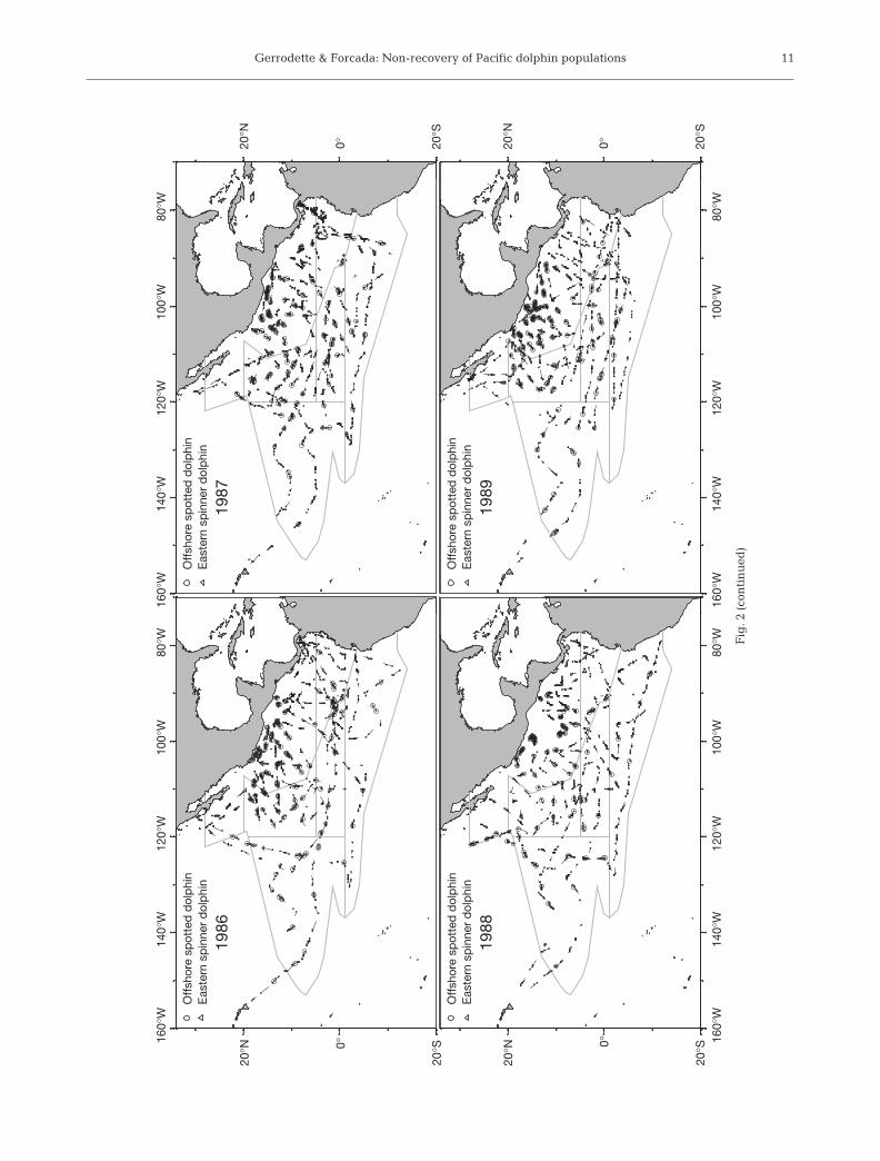
Gerrodette & Forcada: Non-recovery of Pacific dolphin populations 11
1986
Off
shor
e sp
otte
d d
olp
hin
Eas
tern
sp
inne
r d
olp
hin
1987
Off
shor
e sp
otte
d d
olp
hin
Eas
tern
sp
inne
r d
olp
hin
1988
Off
shor
e sp
otte
d d
olp
hin
Eas
tern
sp
inne
r d
olp
hin
1989
Off
shor
e sp
otte
d d
olp
hin
Eas
tern
sp
inne
r d
olp
hin
20°S0°
20°N
20°S0°
20°N
160°
W14
0°W
120°
W10
0°W
80°W
160°
W14
0°W
120°
W10
0°W
80°W
160°
W14
0°W
120°
W10
0°W
80°W
160°
W14
0°W
120°
W10
0°W
80°W
20°S
0°20°N
20°S
0°20°N
Fig
. 2 (
con
tin
ued
)

Mar Ecol Prog Ser 291: 1–21, 200512
1990
Off
shor
e sp
otte
d d
olp
hin
Eas
tern
sp
inne
r d
olp
hin
1998
Off
shor
e sp
otte
d d
olp
hin
Eas
tern
sp
inne
r d
olp
hin
Off
shor
e sp
otte
d d
olp
hin
Eas
tern
sp
inne
r d
olp
hin
1999
Off
shor
e sp
otte
d d
olp
hin
Eas
tern
sp
inne
r d
olp
hin
2000
20°S0°
20°N
20°S
0°20°N
160°
W14
0°W
120°
W10
0°W
80°W
20°S0°
20°N
160°
W14
0°W
120°
W10
0°W
80°W
160°
W14
0°W
120°
W10
0°W
80°W
160°
W14
0°W
120°
W10
0°W
80°W
20°S
0°20°N
Fig
. 2 (
con
tin
ued
)

Gerrodette & Forcada: Non-recovery of Pacific dolphin populations
Trends
Linear weighted least-squares regressions indicatedpositive but small increases for both NE offshorespotted (0.3% yr–1, SE = 0.7%) and eastern spinner(0.1% yr–1, SE = 1.0%) dolphins over the period 1979 to2000 (Fig. 6). Quadratic regressions indicated a con-cave-upward curve for NE offshore spotted dolphins,and a concave-downward curve for eastern spinnerdolphins. None of the regressions was statisticallysignificant at the α = 0.05 level. A weighted LOESSsmooth with span 1.5 through the NE offshore spottedestimates indicated a slight decline through the late1980s and a slight increase (<1% yr–1) since then (Fig.7). A similar smooth through the eastern spinner esti-mates indicated an increasing population until 1990,followed by a decline of 2 to 3% yr–1 until 2000.
Given the number of estimates at the observed inter-vals and variance, the statistical power of detecting a 1,2, 3, 4 or 5% annual rate of change between 1979 and2000 using ordinary least-squares regression was esti-mated to be 0.26, 0.67, 0.95, 1.0 and 1.0, respectively.
DISCUSSION
Abundance
Based on averages of the estimates from the 1998 to2000 surveys, the current size of the NE offshore spot-ted dolphin population is about 640 000 animals, andthe current size of the eastern spinner dolphin popula-tion is about 450 000 animals (Table 3). The estimatesfrom the 3 most recent surveys agreed well with eachother for both populations within the precision of theestimates (CVs of about 17 and 23%, respectively;Fig. 6). The survey effort for eastern spinner dolphinsin the outer stratum was small, relative to the largerange of the dolphin stocks, in 1980, 1982 and 1983,and in 1999–2000 (Fig. 2). Estimates based on thissparse effort were less certain than in other years, andthe bootstrap process probably underestimated thetrue uncertainty in these estimates.
The estimates of NE offshore spotted and easternspinner dolphin abundance prior to 1998 presented inTable 3 differed from past estimates. Although some
13
1979n = 81
1980n = 62
1982n = 45
1983n = 38
1986n = 131
1987n = 140
1988n = 92
1989n = 143
0.6
0.4
0.2
0.0
0.6
0.4
0.2
0.0
Pro
bab
ility
den
sity
0.6
0.4
0.2
0.0
1990n = 122
1998n = 310
1999n = 175
0 1 2 3 4 5 60 1 2 3 4 5 6
Perpendicular distance (km)
0 1 2 3 4 5 60 1 2 3 4 5 6
2000n = 216
Fig. 3. Stenella attenuata. Frequency of sightings by perpendicular distance. Half-normal model fitted to the observations (without covariates)

Mar Ecol Prog Ser 291: 1–21, 2005
estimates were higher and others lower, the main fea-ture was that the estimates presented here were lessvariable among years than previous estimates. The dif-ferences between the old and new estimates were dueto a number of changes, updates and improvements,both to the data and to the analysis. These included:
(1) explicit modeling of other factors (covariates) thataffected probability of detection (Appendix 1); (2) im-plicit handling of school size detection bias; (3) AIC-weighted averaging of estimates from different mod-els; (4) use of the half-normal model for the detectionfunction across all years; (5) bias correction of school
14
600
500
400
300
200
100
0
1979 1980 1982 1983 1986 1987 1988 1989 1990 1998 1999 20001979 1980 1982 1983 1986 1987 1988 1989 1990 1998 1999 2000
Dol
phi
n sc
hool
siz
e
600
500
400
300
200
100
0
Northeastern offshore spotted dolphins Eastern spinner dolphins
Fig. 5. Stenella attenuata attenuata and S. longirostris orientalis. Box-and-whisker plots of school size distributions, with means( ), medians (thick horizontal lines), 95% confidence intervals on the medians (hatched boxes), interquartile ranges (openboxes), and standard spans (whiskers and staples). Thin horizontal lines are outliers; both plots contain additional outliers that are
not shown
1979n = 45
1980n = 30
1982n = 31
1983n = 23
1986n = 99
1987n = 94
1988n = 77
1989n = 100
0 1 2 3 4 5 6 0 1 2 3 4 5 6 0 1 2 3 4 5 6 0 1 2 3 4 5 6
Perpendicular distance (km)
1990n = 66
1998n = 146
1999n = 105
2000n = 102
0.5
0.4
0.3
0.2
0.1
0.0
Pro
bab
ility
den
sity
0.5
0.4
0.3
0.2
0.1
0.0
0.5
0.4
0.3
0.2
0.1
0.0
Fig. 4. Stenella longirostris. Frequency of sightings by perpendicular distance. Half-normal model fitted to the observations (without covariates)

Gerrodette & Forcada: Non-recovery of Pacific dolphin populations
size estimates based on aerial photography; (6) moreaccurate measurements of distance and area; (7) im-proved bootstrap procedures for estimating measuresof precision; and (8) additional checking and editing ofdata for all years. Gerrodette & Forcada (2002) discussthese factors in more detail.
Conventional line-transect methods use perpendicu-lar distance from the trackline to estimate an effectivestrip width and rely on ‘pooling robustness’ to accountfor the multiple factors affecting whether an object isdetected or not (Burnham et al. 1980). While they arewidely used and generally robust, these methods havelimitations (Ramsey & Harrison 2004), and modelingthe effects is an improved approach (Marques & Buck-land 2003, Forcada et al. 2004, Royle et al. 2004). Forthe dolphins considered here, the effects of covariatessuch as school size, sea state and sighting cue, in-
cluding the presence of a bird flock, were importantin modeling the probability of detection of a school(Table 2). Using generalized additive modeling for awide variety of cetaceans, Barlow et al. (2001) alsofound school size, sea state and cue to be importantpredictors of mean perpendicular distance of detec-tion. Similarly, Marques & Buckland (2003), analyzingfishing vessel data for NE offshore spotted dolphins,found school size and sighting cue to be important fac-tors. Sea state did not seem to be an important factor,but this may have been due to the more restrictedrange of Beaufort conditions considered by Marques &Buckland (0 to 3, as opposed to 0 to 5 in this study andin Barlow et al.). Sea state is particularly importantfor less conspicuous species such as harbor porpoisesPhocoena spp. (Jaramillo-Legorreta et al. 1999, Teil-mann 2003).
15
Ab
und
ance
(in
thou
sand
s)
1980 1985 1990 1995 2000
1500
1000
500
0
1500
1000
500
0
Northeastern offshore spotted dolphins
1980 1985 1990 1995 2000
Eastern spinner dolphins
Fig. 6. Stenella attenuata attenuata and S. longirostris orientalis. Estimates of abundance 1979–2000, with 95% confidence intervals (vertical lines), linear model (solid line) and quadratic model (dashed line)
Ab
und
ance
(in
thou
sand
s)
1980 1985 1990 1995 2000
Northeastern offshore spotted dolphinsResearch vessel estimates (this paper)Fishing vessel index, half-normal modelFishing vessel index, modes-of-search modelFishing vessel index, covariate model
1980 1985 1990 1995 2000
Eastern spinner dolphins
Research vessel estimates (this paper)Fishing vessel index, half-normal model
2000
1500
1000
500
0
Fig. 7. Stenella attenuata attenuata and S. longirostris orientalis. Comparison of estimates of abundance 1979–2000, based ondata from research vessel surveys (this study) with indices of abundance based on data collected by observers on fishing vessels.
A weighted LOESS smoothed line is shown for each set of estimates

Mar Ecol Prog Ser 291: 1–21, 2005
Bias
For this study, the key assumptions of line-transectanalysis were:
(1) Objects on the trackline are detected with cer-tainty. For these large dolphin schools, the assumptionis reasonable and generally supported (Brandon et al.2002). However, a small percentage of schools wereprobably missed, leading to a slight underestimation ofabundance.
(2) Objects are detected at their initial location.While these dolphins move away from survey vessels(Au & Perryman 1982), most dolphin schools weresighted with 25× binoculars before they reacted signif-icantly (Hewitt 1985, Brandon et al. 2002). Frequenciesof sightings by perpendicular distance did not indicateavoidance prior to detection (Figs. 3 & 4). Randommovement of schools can cause a positive bias (Hiby1982), but the speed of the vessel was high enoughrelative to normal dolphin movement for this effect tobe small.
(3) Measurements are exact. On a moving ship, mea-surements of angles and distances to sightings are notexact. Use of angle rings and reticle scales improvedaccuracy, and the small systematic underestimation ofdistance due to refraction of light, with resulting over-estimation of abundance, was corrected (Kinzey &Gerrodette 2003). Even without systematic error, vari-ability in distance measurements can lead to under-estimation of abundance (Chen 1998); variability inthis study (Kinzey & Gerrodette 2003) was sufficientlylow for this bias to be small. Exact determination ofdolphin school sizes was not possible. However, theaccuracy of group size estimates in this study wasestablished by comparing estimates with aerial pho-tographs. The general tendency to underestimategroup size, with resulting negative bias in abundanceestimates, was reduced by calibrating the estimates ofindividual observers (Gerrodette et al. 2002).
These surveys were conducted in closing mode,meaning that the ship left the trackline to approachdolphin sightings. This break in search effort was nec-essary to identify species and obtain accurate schoolsize estimates, but may lead to undersampling of highdensity areas. Estimates of abundance using closingmode were negatively biased compared to passingmode, in which the ship does not leave the trackline,for Antarctic minke whales (Haw 1991, Branch & But-terworth 2001a), but positively biased for most othercetaceans (Branch & Butterworth 2001b). In surveysup to 1990, we closed on spotted and spinner schoolsonly, whereas in 1998 to 2000, we closed on allcetacean sightings within 3 n miles of the trackline.Because spotted and spinner dolphins have differenthabitat characteristics than other dolphins (Reilly &
Fiedler 1994), this implies that the effect would havebeen weaker in the 1998 to 2000 surveys than earlier, ifclosing mode does create a negative bias by under-sampling.
Trends and recovery
Contrary to the claim of Hall et al. (2000, p 210) that‘recovery [of these dolphin stocks] is under way,’ thedata show that the stocks are not recovering at ratesconsistent with the estimated levels of depletion andcurrent low reported levels of bycatch. Dolphin popu-lations are estimated to be capable of growing at 4%yr–1 or more (Reilly & Barlow 1986). For both stocks, theestimates did not show any statistically significanttrend, either upwards or downwards, during the 21 yrperiod (Fig. 6). The power analysis showed that if thedolphin populations had been growing (or declining)at a rate of ≥ 3% yr–1 from 1979 to 2000, there was highpower (>0.95) to detect that change. There was inter-mediate power (0.67) to detect a 2% yr–1 change, andlow power (0.26) to detect a 1% yr–1 change. Thus, thenon-significant regression analysis was not very infor-mative about the smaller rates of change, as the stan-dard errors also indicated. The lack of recovery ofthese dolphin stocks is in sharp contrast to 3 decades ofactions (Gosliner 1999, Hall et al. 2000), which havereduced the dolphin bycatch by 2 orders of magnitude,from several hundred thousand dolphins per year(Wade 1995) to <2000 (Bayliff 2004).
Lennert-Cody et al. (2001) reached a similar conclu-sion about the lack of recovery based on analysis ofdata collected by observers on the fishing vessels. ForNE offshore spotted dolphins, several indices of abun-dance were calculated, including estimates based on aunivariate half-normal model (Lennert-Cody et al.2001), a modes-of-search model which stratified dataaccording to searching method (Lennert-Cody et al.2001), and a sighting-covariate model (Marques 2001).For this stock, all fishing vessel indices showed anincreasing population until about 1990, followed by adecline (Fig. 7). In contrast, the research vessel esti-mates (this study) did not indicate a decline in the lastdecade. For eastern spinner dolphins, the fishingvessel index was based on the half-normal model onlyand showed a similar trajectory to the estimatesreported in this study (Fig. 7). Indices were positivelycorrelated with abundance estimates for both NE off-shore spotted and eastern spinner dolphins (r = 0.34,SE = 0.30 and r = 0.51, SE = 0.27, respectively). For allindices derived from fishing vessel data, Lennert-Codyet al. (2001) cautioned that the data contain time-varying biases. After considering the possible size ofthese biases, however, the authors concluded that ‘it
16

Gerrodette & Forcada: Non-recovery of Pacific dolphin populations
seems unlikely that either of the stocks … are in-creasing at rates that might be expected if they hadbeen well below carrying capacity through the 1980s’(p 318).
Hypotheses for lack of recovery
There are several possible reasons why the dolphinpopulations are not recovering at expected rates.
(1) Dolphin bycatch is higher than reported. TheInter-American Tropical Tuna Commission, the fish-eries commission which runs the international ob-server program and produces the bycatch estimates,reports that recent dolphin bycatch is known withouterror (Bayliff 2004). Observer coverage is close to100% for the large (>363 mt) vessels which set on dol-phins. Nevertheless, the reported number of dolphinskilled is an underestimate, because: (a) smaller boats,which may sometimes set on dolphins, do not haveobservers; (b) observers do not see all of the net at alltimes on all sets; (c) some injured dolphins may dielater (observers record ‘severely injured’ dolphins asmortalities); (d) dead dolphins, when observed, maynot always be reported. The magnitude of under-reporting due to these effects is not known. Further-more, there is unobserved mortality of orphaned calveswhen lactating females are killed without their calves(Archer et al. 2004).
(2) Effects of the fishery go beyond bycatch. Theannual number of dolphins chased, captured andreleased during fishing operations is high (Archer et al.2002). Individual NE offshore spotted dolphins interactwith the fishery between 2 and 50 times yr–1, depend-ing on size of the school (Perkins & Edwards 1999). It islikely that this rate of interaction has negative effectson survival and/or reproduction through stress (Curry1999, Appendix 7 in Reilly et al. 2005), increased pre-dation (Perryman & Foster 1980), and separation ofmothers and calves (Archer et al. 2001). Separation ofmothers and calves may be due to disruption of thehydrodynamic drafting relationship between motherand calf during chase (Weihs 2004). In response tofishing activity, ETP dolphins have changed their be-havior, becoming more evasive (Schramm Urrutia1997, Heckel et al. 2000, Mesnick et al. 2002, San-turtún Oliveros & Galindo Maldonado 2002, Lennert-Cody & Scott 2005). Seemingly small changes inbehavior can have strong demographic effects (Ger-rodette & Gilmartin 1990). Differences in testes sizeindicate that eastern spinner dolphins have a morestructured mating system than other subspecies ofspinner dolphins, which may make them more vulner-able to frequent harassment (Perrin & Mesnick 2003).Calf production has been declining since 1987 for both
eastern spinner and NE offshore spotted dolphins (K.Cramer, W. Perryman, T.G. unpubl.). Although thereare many probable cryptic effects of the fishery on dol-phin vital rates, the actual magnitudes of these effectsare not known.
(3) Dolphin habitat is not constant. NE offshore spot-ted and eastern spinner dolphins occur in the warm,stratified waters of the central part of the ETP (Reilly &Fiedler 1994). Decadal-scale ‘regime shifts’ have beendescribed in the North Pacific (Francis et al. 1998, Hare& Mantua 2000, Chavez et al. 2003) and equatorialPacific (McPhaden & Zhang 2002). In the ETP, how-ever, decadal variability is relatively low, El Niño-scalevariability (2 to 7 yr) predominates, and average pri-mary production does not appear to have declinedsince the late 1960s (Fiedler 2002). Since these dolphinpopulations are currently at 20 to 30% of their pre-fishery levels (Wade et al. 2002), a large decline indolphin habitat would be necessary to explain the lackof dolphin recovery. Such a large change is not indi-cated by temporal patterns in oceanographic variables,ichthyoplankton, fish, squid, seabirds, other cetaceans,or dolphin habitat (reviewed in Appendix 6 of Reilly etal. 2005), although biological data are not availableprior to 1986. A longer time-series from the fisheryindicates an increase around 1985 in the abundance ofyellowfin tuna (Maunder & Harley 2004), which mayindicate a change to more, not less, favorable habitat atthat time for dolphins that associate with the tuna.Nevertheless, given fragmentary data and our limitedunderstanding of how environmental changes affectdolphin abundance, we cannot rule out that ecosystemchanges have negatively affected the recovery of thedolphin populations.
(4) Expectations of immediate recovery are over-simplified. Relatively simple single-species populationmodels do not account for a variety of factors thatmight lead to a delay in, or perhaps even a failure of,dolphin recovery. Such factors could include competi-tive displacement by fish, sharks, or other cetaceans,depensatory (‘Allee’) effects at low population sizes,and disruptions to the age or social structure by pastdolphin bycatch. Fisheries have a wide variety ofeffects on marine ecosystems (Dayton et al. 1995, Jen-nings & Kaiser 1998, Pauly et al. 1998). In the oligo-trophic ETP, competitive interactions are important instructuring the seabird community (Ballance et al.1997), but other interspecific dynamics are poorlyknown. Most centrally, the ecological association ofdolphins and yellowfin tuna, which forms the basis ofthe fishery, is still so little understood that we do notknow whether the large removal of tuna biomass bythe fishery in the last 40 yr has had a positive, negativeor neutral effect on dolphin population dynamics.Hutchings (2000) noted little evidence of recovery in
17

Mar Ecol Prog Ser 291: 1–21, 2005
90 fish stocks after >15 yr since fishing was reduced.On the other hand, Best (1993) described recovery inmost baleen whale stocks after cessation of whaling.Modeling of the ETP ecosystem (Watters et al. 2003)may provide some insights about the effects of inter-specific interactions as well as environmental changeon recovery.
These hypotheses are not mutually exclusive. Morethan one may be responsible for the lack of dolphin re-covery. Continued monitoring and ongoing research areaimed at evaluating which factors are most important.
Acknowledgements. Projects of this magnitude rely onthe cooperative work of many people over many years.T. D. Smith led dolphin assessment studies in the 1970s.D. W. K. Au (1979), R. S. Holt (1980–1988), and L. T. Ballance(1999–2000) were chief scientists for the cruises (T.G. waschief scientist in other years). We collectively thank thedozens of observers who collected the data, the cruise leaderson various legs of the cruises, and the officers and crews of theresearch vessels. At the Southwest Fisheries Science Center,thanks to colleagues J. P. Barlow, J. R. Brandon, K. L. Cramer,R. C. Holland, A. R. Jackson, S. L. Martin, W. L. Perryman,and S. B. Reilly. The analysis benefited from the input of S. T.Buckland and T. Schweder at an October 2000 review spon-sored by the Inter-American Tropical Tuna Commission. Thefinal manuscript was improved by comments by T. D. Smith,W. F. Perrin, S. J. Chivers, P. C. Fiedler, and 3 anonymousreviewers. The 1998–2000 surveys were supported by theU.S. International Dolphin Conservation Program Act.
LITERATURE CITED
Archer F, Gerrodette T, Dizon A, Abella K, Southern 2 (2001)Unobserved kill of nursing dolphin calves in a tuna purse-seine fishery. Mar Mamm Sci 17:540–554
Archer F, Gerrodette T, Jackson A (2002). Preliminary esti-mates of the annual number of sets, number of dolphinschased, and number of dolphins captured by stock in thetuna purse-seine fishery in the eastern tropical Pacific,1971–2000. Admin Rep LJ-02-10, Southwest FisheriesScience Center, La Jolla (available at: swfsc.ucsd.edu/IDCPA/TunaDol_rep)
Archer F, Gerrodette T, Chivers S, Jackson A (2004) Annualestimates of the unobserved incidental kill of pantropicalspotted dolphin (Stenella attenuata attenuata) calves inthe tuna purse-seine fishery of the eastern tropical Pacific.Fish Bull 102:233–244
Au D, Perryman W (1982) Movement and speed of dolphinschools responding to an approaching ship. Fish Bull 80:371–379
Au DWK, Pitman RL (1986) Seabird interactions with dolphinsand tuna in the eastern tropical Pacific. Condor 88:304–317
Ballance LT, Pitman RL, Reilly SB (1997) Seabird communitystructure along a productivity gradient: importanceof competition and energetic constraint. Ecology 78:1502–1518
Barlow J, Gerrodette T, Perryman W (1998). Calibratinggroup size estimates for cetaceans seen on ship surveys.Admin Rep LJ-98-11, Southwest Fisheries Science CenterLa Jolla (available at: swfsc.ucsd.edu/IDCPA/TunaDol_rep)
Barlow J, Gerrodette T, Forcada J (2001) Factors affecting
perpendicular sighting distances on shipboard line-transect surveys for cetaceans. J Cetacean Res Manag3:201–212
Bayliff WH (ed) (2004) 2002 annual report. Inter-AmericanTropical Tuna Commission, La Jolla
Best PB (1993) Increase rates in severely depleted stocks ofbaleen whales. ICES J Mar Sci 50:169–186
Borchers DL, Buckland ST, Goedhart PW, Clarke ED, HedleySL (1998) Horvitz-Thompson estimators for double-platform line transect surveys. Biometrics 54:1221–1237
Borchers DL, Buckland ST, Zucchini W (2002) Estimatinganimal abundance: closed populations. Springer-Verlag,London
Branch TA, Butterworth DS (2001a) Southern hemisphereminke whales: standardised abundance estimates fromthe 1978/79 to 1997/98 IDCR-SOWER surveys. J CetaceanRes Manag 3:143–174
Branch TA, Butterworth DS (2001b) Estimates of abundancesouth of 60°S for cetacean species sighted frequently onthe 1978/79 to 1997/98 IWC/IDCR-SOWER sighting sur-veys. J Cetacean Res Manag 3:251–270
Brandon J, Gerrodette T, Perryman W, Cramer K (2002). Re-sponsive movement and g(0) for target species of researchvessel surveys in the eastern tropical Pacific Ocean.Admin Rep LJ-02-02, Southwest Fisheries Science Center,La Jolla (available at: swfsc.ucsd.edu/IDCPA/TunaDol_rep)
Buckland ST (1992) Maximum likelihood fitting of hermiteand simple polynomial densities. Appl Stat 41:241–266
Buckland ST, Anderson DR, Burnham KP, Laake JL, BorchersDL, Thomas L (2001) Introduction to distance sampling:estimating abundance of biological populations. OxfordUniversity Press, New York
Burnham KP, Anderson DR (1998) Model selection andinference: a practical information-theoretic approach.Springer-Verlag, New York
Burnham KP, Anderson DR, Laake JL (1980) Estimation ofdensity from line transect sampling of biological popula-tions. Wildl Monogr 72:1–202
Chavez FP, Ryan J, Lluch-Cota SE, Ñiquen CM (2003) Fromanchovies to sardines and back: multidecadal change inthe Pacific Ocean. Science 299:217–221
Chen SX (1998) Measurement errors in line transect surveys.Biometrics 54:899–908
Curry BE (1999) Stress in mammals: the potential influence offishery-induced stress on dolphins in the eastern tropicalPacific Ocean. NOAA Tech Memo NMFS-SWFSC-260,NOAA, La Jolla
Davison AC, Hinkley DV (1997) Bootstrap methods and theirapplication. Cambridge University Press, Cambridge
Dayton PK, Thrush SF, Agardy MT, Hofman RJ (1995)Environmental effects of marine fishing. Aquat Conserv5:205–232
Dizon AE, Perrin WF, Akin PA (1994). Stocks of dolphins(Stenella spp. and Delphinus delphis) in the eastern tropi-cal Pacific: a phylogeographic classification. NOAA TechRep NMFS 119, US Dept of Commerce, Seattle
Edwards EF, Perkins PC (1998) Estimated tuna discard fromdolphin, school, and log sets in the eastern tropical PacificOcean, 1989–1992. Fish Bull 96:210–222
Efron B, Tibshirani R (1993) An introduction to the bootstrap.Chapman & Hall, New York
Fiedler PC (2002) Environmental change in the easterntropical Pacific Ocean: review of ENSO and decadal vari-ability. Admin Rep LJ-02-16, Southwest Fisheries ScienceCenter, La Jolla (available at: swfsc.ucsd.edu/IDCPA/TunaDol_rep)
Forcada J (2002) Multivariate methods for size-dependent
18

Gerrodette & Forcada: Non-recovery of Pacific dolphin populations
detection in conventional line transect sampling. AdminRep LJ-02-07, Southwest Fisheries Science Center, La Jolla(available at: swfsc.ucsd.edu/IDCPA/TunaDol_rep)
Forcada J, Gazo M, Aguilar A, Gonzalvo J, Fernández-Contr-eras M (2004) Bottlenose dolphin abundance in the NWMediterranean: addressing heterogeneity in distribution.Mar Ecol Prog Ser 275:275–287
Francis RC, Hare SR, Hollowed AB, Wooster WS (1998)Effects of interdecadal climate variability on the oceanicecosystems of the NE Pacific. Fish Oceanogr 7:1–21
Gerrodette T (1987) A power analysis for detecting trends.Ecology 68:1364–1372
Gerrodette T (1993) TRENDS: software for a power analysis oflinear regression. Wildl Soc Bull 21:515–516
Gerrodette T (2002) The tuna–dolphin issue. In: Perrin WF,Würsig B, Thewissen JGM (eds) Encyclopedia of marinemammals. Academic Press, San Diego, p 1269–1273
Gerrodette T, Forcada J (2002) Estimates of abundance ofnortheastern offshore spotted, coastal spotted, and easternspinner dolphins in the eastern tropical Pacific Ocean.Admin Rep LJ-02-06, Southwest Fisheries Science Center,La Jolla (available at: swfsc.ucsd.edu/IDCPA/TunaDol_rep)
Gerrodette T, Gilmartin WG (1990) Demographic conse-quences of changed pupping and hauling sites of theHawaiian monk seal. Conserv Biol 4:423–430
Gerrodette T, Perryman W, Barlow J (2002) Calibrating groupsize estimates of dolphins in the eastern tropical PacificOcean. Admin Rep LJ-02-08, Southwest Fisheries ScienceCenter, La Jolla (available at: swfsc.ucsd.edu/IDCPA/TunaDol_rep)
Gilpatrick JW Jr (1993) Method and precision in estimation ofdolphin school size with vertical aerial photography. FishBull 91:641–648
Gordon JCD (1990) A simple photographic technique formeasuring the length of whales from boats at sea. Rep IntWhal Comm 40:581–588
Gosliner ML (1999) The tuna–dolphin controversy. In: TwissJR Jr, Reeves RR (eds) Conservation and management ofmarine mammals. Smithsonian Institution Press, Washing-ton, DC, p 120–155
Hall MA (1998) An ecological view of the tuna–dolphin prob-lem: impacts and trade-offs. Rev Fish Biol Fish 8:1–34
Hall MA, Alverson DL, Metuzals KI (2000) By-catch: problemsand solutions. Mar Poll Bull 41:204–219
Hare SR, Mantua NJ (2000) Empirical evidence for NorthPacific regime shifts in 1977 and 1989. Prog Oceanogr47:103–145
Haw MD (1991) An investigation into the differences inminke whale school density estimates from passing modeand closing mode survey in IDCR Antarctic assessmentcruises. Rep Int Whal Comm 41:313–330
Hayes RJ, Buckland ST (1983) Radial distance models for theline transect method. Biometrics 39:29–42
Heckel G, Murphy KE, Compeán Jiménez GA (2000) Evasivebehavior of spotted and spinner dolphins (Stenella attenu-ata and S. longirostris) during fishing for yellowfin tuna(Thunnus albacares) in the eastern Pacific Ocean. FishBull 98:692–703
Hedley C (2001) The 1998 Agreement on the InternationalDolphin Conservation Program: recent developments inthe tuna–dolphin controversy in the eastern PacificOcean. Ocean Dev Int Law 32:71–92
Hewitt RP (1985) Reaction of dolphins to a survey vessel:effects on census data. Fish Bull 83:187–193
Hiby AR (1982) The effect of random whale movement ondensity estimates obtained from whale sighting surveys.Rep Int Whal Comm 32:791–793
Holt RS, Gerrodette T, Cologne JB (1987) Research vessel sur-vey design for monitoring dolphin abundance in the east-ern tropical Pacific. Fish Bull 85:435–446
Hoyle SD, Maunder MN (2004) A Bayesian integrated pop-ulation dynamics model to analyze data for protectedspecies. Anim Biodiv Conserv 27.1:247–266
Hurvich CM, Tsai CL (1989) Regression and time series modelselection in small samples. Biometrika 76:297–307
Hutchings JA (2000) Collapse and recovery of marine fishes.Nature 406:882–885
Jaramillo-Legorreta AM, Rojas-Bracho L, Gerrodette T (1999)A new abundance estimate for vaquitas: first step forrecovery. Mar Mamm Sci 15:957–973
Jennings S, Kaiser MJ (1998) The effects of fishing on marineecosystems. Adv Mar Biol 34:201–352
Joseph J (1994) The tuna–dolphin controversy in the easternPacific Ocean: biological, economic, and political impacts.Ocean Dev Int Law 25:1–30
Kinzey D, Gerrodette T (2001) Conversion factors for binocu-lar reticles. Mar Mamm Sci 17:353–361
Kinzey D, Gerrodette T (2003) Distance measurements usingbinoculars from ships at sea: accuracy, precision andeffects of refraction. J Cetacean Res Manag 5:159–171
Kinzey D, Olson P, Gerrodette T (2000) Marine mammal datacollection procedures on research ship line-transectsurveys by the Southwest Fisheries Science Center.Admin Rep LJ-00-08, Southwest Fisheries Science Center,La Jolla (available at: swfsc.ucsd.edu/IDCPA/TunaDol_rep)
Lennert-Cody CE, Scott MD (2005) Spotted dolphin evasiveresponse in relation to fishing effort. Mar Mamm Sci 21:13–28
Lennert-Cody CE, Buckland ST, Marques FFC (2001) Trendsin dolphin abundance estimated from fisheries data: acautionary note. J Cetacean Res Manag 3:305–319
Lerczak JA, Hobbs RC (1998) Calculating sighting distancesfrom angular readings during shipboard, aerial and shore-based marine mammal surveys. Mar Mamm Sci 14:590–599
Marques FFC (2001) Estimating wildlife distribution andabundance from line transect surveys conducted fromplatforms of opportunity. PhD thesis. University of St.Andrews
Marques FFC, Buckland ST (2003) Incorporating covariatesinto standard line transect analyses. Biometrics 59:924–935
Maunder MN, Harley SJ (2004) Status of yellowfin tuna in theeastern Pacific Ocean in 2002 and outlook for 2003. IATTCStock Assess Rep 4:5–91
McPhaden MJ, Zhang D (2002) Slowdown of the meridionaloverturning circulation in the upper Pacific Ocean. Nature415:603–608
Mesnick SL, Archer FI, Allen AC, Dizon AE (2002) Evasivebehavior of eastern tropical Pacific dolphins relative toeffort by the tuna purse-seine fishery. Admin Rep LJ-02-30, Southwest Fisheries Science Center, La Jolla (availableat: swfsc.ucsd.edu/IDCPA/TunaDol_rep)
NRC (National Research Council) (1992) Dolphins and thetuna industry. National Academy Press, Washington, DC
Pauly D, Christensen V, Dalsgaard J, Froese R, Torres F Jr(1998) Fishing down marine food webs. Science 279:860–863
Perkins PC, Edwards EF (1999) Capture rate as a function ofschool size in pantropical spotted dolphins, Stenella atten-uata, in the eastern tropical Pacific Ocean. Fish Bull97:542–554
Perrin WF (1990) Subspecies of Stenella longirostris (Mam-malia: Cetacea: Delphinidae). Proc Biol Soc Wash 103:453–463
Perrin WF, Mesnick SL (2003) Sexual ecology of the spinner
19

Mar Ecol Prog Ser 291: 1–21, 2005
dolphin, Stenella longirostris: geographic variation in mat-ing system. Mar Mamm Sci 19:462–483
Perrin WF, Schnell GD, Hough DJ, Gilpatrick JW Jr, Kashi-wada JV (1994) Reexamination of geographic variation incranial morphology of the pantropical spotted dolphin,Stenella attenuata, in the eastern Pacific. Fish Bull 92:324–346
Perryman WL, Foster TC (1980) Preliminary report on preda-tion by small whales, mainly the false killer whale,Pseudorca crassidens, on dolphins (Stenella spp. and Del-phinus delphis) in the eastern tropical Pacific. Admin RepLJ-80-05, Southwest Fisheries Science Center, La Jolla(available at: swfsc.ucsd.edu/IDCPA/TunaDol_rep)
Quinn TJ II, Gallucci VF (1980) Parametric models for line-transect estimators of abundance. Ecology 61:293–302
Ramsey FL, Harrison K (2004) A closer look at detectability.Environ Ecol Stat 11:73–84
Ramsey FL, Wildman V, Engbring J (1987) Covariate adjust-ments to effective area in variable-area wildlife surveys.Biometrics 43:1–11
Reilly SB (1990) Seasonal changes in distribution and habitatdifferences among dolphins in the eastern tropical Pacific.Mar Ecol Prog Ser 66:1–11
Reilly SB, Barlow J (1986) Rates of increase in dolphin popu-lation size. Fish Bull 84:527–533
Reilly SB, Fiedler PC (1994) Interannual variability of dolphinhabitats in the eastern tropical Pacific. I: Research vesselsurveys, 1986–1990. Fish Bull 92:434–450
Reilly SB, Donahue MA, Gerrodette T, Forney K and 8 others(2005) Report of the scientific research program under theInternational Dolphin Conservation Program Act. NOAATech Memo NMFS-SWFSC-372. (also available at http://swfsc.nmfs.noaa.gov/IDCPA/TunaDol_rep/)
Royle JA, Dawson DK, Bates S (2004) Modeling abundanceeffects in distance sampling. Ecology 85:1591–1597
Santurtún Oliveros E, Galindo Maldonado F (2002) Copingbehaviors of spotted dolphins during fishing sets. AdminRep LJ-02-36C, Southwest Fisheries Science Center, La
Jolla (available at: swfsc.ucsd.edu/IDCPA/TunaDol_rep)Schramm Urrutia Y (1997) Nivel de actividad de los delfines
manchado Stenella attenuata y tornillo oriental S. lon-girostris, en redes atuneras, en el Océano Pacífico Orien-tal. MS thesis, Universidad Autónoma de Baja California,Ensenada, BC
Smith TD (1983) Changes in size of three dolphin (Stenellaspp.) populations in the eastern tropical Pacific. Fish Bull81:1–13
Teilmann J (2003) Influence of sea state on density estimatesof harbour porpoises (Phocoena phocoena). J CetaceanRes Manag 5:85–92
Wade PR (1993) Estimation of historical population size of theeastern spinner dolphin (Stenella longirostris orientalis).Fish Bull 91:775–787
Wade PR (1995) Revised estimates of incidental kill ofdolphins (Delphinidae) by the purse-seine tuna fishery inthe eastern tropical Pacific, 1959–1972. Fish Bull 93:345–354
Wade PR, Gerrodette T (1992) Estimates of dolphin abun-dance in the eastern tropical Pacific: preliminary analysisof 5 years of data. Rep Int Whal Comm 42:533–539
Wade PR, Gerrodette T (1993) Estimates of cetacean abun-dance and distribution in the eastern tropical Pacific. RepInt Whal Comm 43:477–493
Wade PR, Reilly SB, Gerrodette T (2002) Assessment of thepopulation dynamics of the northeast offshore spottedand the eastern spinner dolphin populations through2002. Admin Rep LJ-02-13, Southwest Fisheries ScienceCenter, La Jolla (available at: swfsc.ucsd.edu/IDCPA/TunaDol_rep)
Watters GM, Olson RJ, Francis RC, Fiedler PC and 7 others(2003) Physical forcing and the dynamics of the pelagicecosystem in the eastern tropical Pacific: simulations withENSO-scale and global-warming climate drivers. Can JFish Aquat Sci 60:1161–1175
Weihs D (2004) The hydrodynamics of dolphin drafting. J Biol 3:8
20

Gerrodette & Forcada: Non-recovery of Pacific dolphin populations 21
Editorial responsibility: Otto Kinne (Editor-in-Chief), Oldendorf/Luhe, Germany
Submitted: October 8, 2004; Accepted: January 15, 2005Proofs received from author(s): April 20, 2005
Appendix 1. Detection function models and abundance estimators
The multivariate detection probability model g (x,c) isdefined as the conditional probability of sighting a dolphingroup given its perpendicular distance x from the transectline and c, a vector with its size (number of individuals) andadditional detection covariates (sea state, sighting cue, sur-vey platform, etc). Perpendicular distances are assumed tofollow a uniform distribution between the transect line andtruncation distance W: x~I (0,W). With transect lines allo-cated randomly in the survey area, perpendicular distancesare assumed to be independent of group size and othercovariates. Thus, the unconditional probability of detectinga group is
(A1)
where ƒ(x,c) is the joint probability density function (pdf) ofobserved perpendicular distances and group size and addi-tional covariates, c, expressed as
(A2)
This function requires knowledge of the form of ƒ(c). Inorder to avoid this problem the function is better expressedas a conditional pdf of x given c, i.e., ƒ(x |c), as
(A3)
The integral in Eq. (A3) is μ(c), the effective strip half-widthunder conditions c, which divided byW is the average prob-ability that a dolphin school with covariates c is detected.
Assuming perfect detection on the transect line, the condi-tional pdf can be evaluated at 0 to estimate μ(c)
(A4)
Estimates ƒ(0|c) were obtained with conditional multivariatedetection function models in which covariates affect the scaleparameter (Ramsey et al. 1987, Forcada 2002, Marques &
ƒ( | )( | )ˆ ( ) ˆ ( )
00 1
cg c
c c= =
μ μ
ƒ( | )( , )
( , )
( , )( )
x cg x c
g x c x
g x ccW
= =∫ d
0
μ
ƒ( , )( , )ƒ( )
( , )ƒ( )x c
g x c c
g x c c x cW
=∫∫ d d
P g x c x c x c W g x c cW W
( , )ƒ( , ) ( , )ƒ( )= =∫∫ ∫∫−d d 1 dd dx c
Buckland 2003). Covariates c were assumed to have multi-plicative effects (additive in a log scale) of the form
(A5)
in 2 competing parametric models, the hazard rate detectionmodel (Hayes & Buckland 1983)
(A6)
where b is a shape parameter, and the half-normal model(Quinn & Gallucci 1980)
(A7)
Horvitz-Thompson-like (Borchers et al. 1998) line-transectestimators have the general form
(A8)
where A is the total area, aw = 2LW is the area surveyed,obtained by combining total transect length L and right-truncation distance W, and E is the expectation operator.Inverse detection probabilities p are summed over the ndetected groups during the sampling of area A.
Expressed as a conditional probability, from Eqs. (A1) to(A3),
(A9)
Using this term in Eq. (A8), the abundance of dolphinschools is
(A10)
and the estimators of dolphin abundance and bias-correctedmean group size are derived similarly.
ˆ ƒ ( | )NAL
ci ii
n
==
∑20
1
E p x c W g x c x
W c
W c
W| ( | )
ƒ( |
( )[ ] =
= ( )
=
−
−
∫1
0
1
0
d
μ
))[ ] −1
ˆ,
NAa E p x cw i ii
n
=( )[ ]=
∑ 1
1
g x cxc
( | ) exp( )
= − ⎡⎣⎢
⎤⎦⎥
⎧⎨⎩
⎫⎬⎭
12
2
α
g x cxc
b
( | ) exp( )
= − −⎡⎣⎢
⎤⎦⎥
⎧⎨⎩
⎫⎬⎭
−
1α
α α α( ) exp log( )c ckk
k= +{ }∑0


![Predictive Modeling of Spinner Dolphin (Stenella ... · spinner), S.l. centroamericana (Central American spinner) and S.l. roseiventris (Dwarf spinner) [19,20]. The Gray’s spinner](https://static.fdocuments.in/doc/165x107/5f87e3e5d2d3037d75174768/predictive-modeling-of-spinner-dolphin-stenella-spinner-sl-centroamericana.jpg)