Non-LTE stellar parameters and abundances of metal-poor ...

Non-LTE stellar parameters and abundances of metal-poor stars in the Galaxy

Rana Ezzeddine (JINA-CEE /MIT postdoctoral fellow)

Photo: Magellan Twin Telescopescredit: Yuri Beletzky

@AstroRana

Cosmic Timeline (Not to Scale)

massive First Stars

0 s~300 MyrsNow: 13.7 Gyrs

First Supernovae

low mass (0.6-0.8Mo) metal-poor stars

First Galaxies

low mass Pop II (metal-poor) stars still around

~1 Gyr

Pop I and Pop II stars in the Milky way

Big Bang

▸ Stellar Archeology: uses stellar relics of the early universe.

▸ Most metal-poor stars preserve records of “First” Population III stars in their atmospheres

Refresher: What are Metal-poor stars?

Metals Z

Periodic TableAstronomers’

H: X He: Y

Withtime,moreandmoreofallelementsweremade!


RANA EZZEDDINE COOL STARS 20 1/AUGUST/2018

๏ Metal-poor [Fe/H] < -1

๏ Very metal-poor (VMP)-3 < [Fe/H] < -2

๏ Extremely metal-poor (EMP) -4 < [Fe/H] < -3

๏ Ultra metal-poor (UMP) -5 < [Fe/H] < -4

๏ Hyper metal-poor (HMP)[Fe/H] < -5

๏ Mega metal-poor (MMP) [Fe/H] < -7 (Keller star 2014)

๏ Ridiculously metal-poor [Fe/H] < -10 Beers & Christlieb (2005) Frebel (2018)



ABUNDANCES ARE ONLY AS GOOD AS THEIR MODELS

B. Gustafsson, Astronomical Observatory, Uppsala (2009)

Abundances are not measured BUT determined using approximations: ๏ Plane-parallel vs. spherical ๏ Homogeneity ๏ Stationarity ๏ Hydrostatic equilibrium ๏1D vs. 3D atmospheres

๏ Local thermodynamic equilibrium (LTE)

REFRESHER: SPECTRAL LINE FORMATION

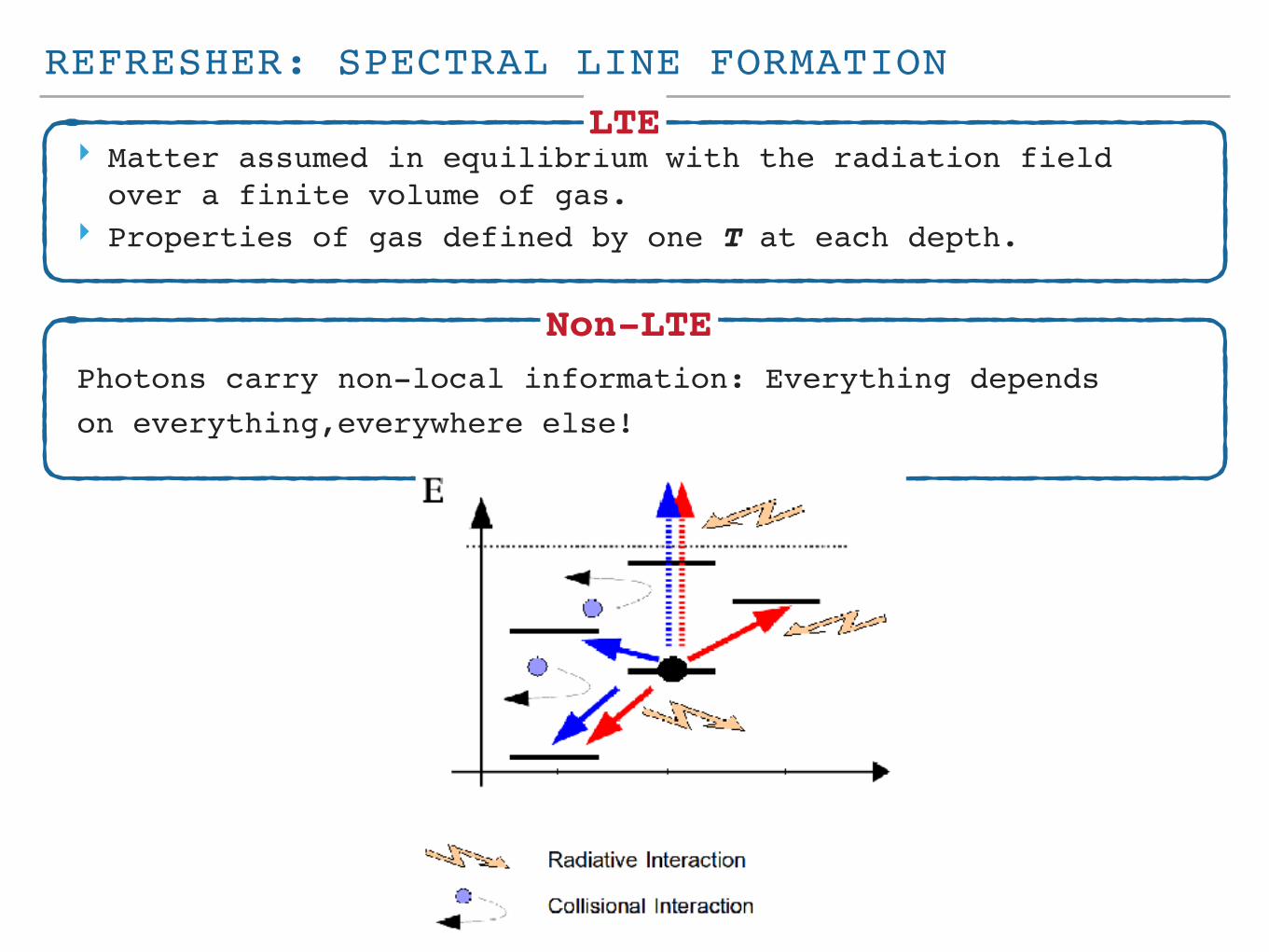
‣ Matter assumed in equilibrium with the radiation field over a finite volume of gas.

‣ Properties of gas defined by one T at each depth.

LTE

REFRESHER: SPECTRAL LINE FORMATION

‣ Matter assumed in equilibrium with the radiation field over a finite volume of gas.

‣ Properties of gas defined by one T at each depth.

LTE

Non-LTEPhotons carry non-local information: Everything depends on everything,everywhere else!

LTE VS NLTE

LTE Fe I

nlow

nhigh1 line : 1 transition

LTE VS NLTE

RANA EZZEDDINE (UNIVERSITE DE MONTPELLIER) PHD PRESENTATION DECEMBER 7th , 2015 31 / 57

Rana Ezzeddine, PhD, 2015 FORMATO2.0 (Merle et al. in prep)

NLTE

LTE

1 line : 81,162 transitions!

1 line : 1 transition

nlow

nhigh

Fe I

Energy

Atomic levels

LTE VS NLTE

LTE


nlow

nhigh

Fe II

LTE VS NLTE

RANA EZZEDDINE (UNIVERSITE DE MONTPELLIER) PHD PRESENTATION DECEMBER 7th , 2015 31 / 57

NLTE

LTE

1 line : 56,981 transitions


nlow

nhigh

Fe II

Energy

Atomic levels

Rana Ezzeddine, PhD, 2015 FORMATO2.0 (Merle et al. in prep)

NON-LOCAL THERMODYNAMIC EQUILIBRIUM EFFECTS

Ezzeddine et al 2017a

level population density (NLTE) level population density (LTE)

Deviations from LTE increase toward lower metallicities

LTE

NLTE

departure coefficient =

NLTE NLTE

NLTE EFFECTS : STELLAR PARAMETERS

20 Standardmetal-poor halo stars

Ezzeddine et al. (in prep)

NLTE EFFECTS : IRON

10

dance uncertainties because the standard errors of Fe Iwould be unrealistically small (e.g., 0.02 and less). (�stdv)are reported in Table 2. Second, systematic uncertain-ties arising from varying the stellar parameters Te↵ , log gand ⇠t by about their uncertainty of ±100K, ±0.2 cgsand ±0.2km s�1 respectively. The resulting changes inthe average Fe abundances typically are ±0.07dex in Fe Iand ±0.01dex for Fe II for changes in changes in Te↵ ,±0.05dex for Fe I and ±0.2dex for Fe II for changes inlog g and finally ±0.1dex for Fe I and ±0.02dex for Fe IIfor changes in ⇠t. Total Fe abundance uncertainties areobtained by summing individual uncertainties (�std and�sys) in quadrature. This leads to a typical total averagevalue of 0.13 dex.

Similarly, the total uncertainties in the other stellar pa-rameters are obtained by summing individual uncertain-ties (�fit, �slope, and �var) in quadrature. This leads totypical total uncertainties of 112 K in Te↵ , 0.45 dex in log gand 0.4 km s�1in ⇠t. These uncertainties well reflect thechallenge of having available only a limited number of Felines in these most iron-poor stars.

5. NLTE CORRECTIONS

We now discuss the differences between our NLTE and LTEiron abundances [Fe/H] for the UMP stars. We also report thedifferences between previously determined stellar parameters(Te↵ , log g and ⇠t) from the literature (where either full LTEor partial LTE and photometric methods were used). TheseNLTE corrections for [Fe/H] are shown in Table 2, while thosefor log g, Te↵ and ⇠t are listed in Table 1.

5.1. [Fe/H] abundance corrections

We define the NLTE Fe line abundance correction for a spe-cific spectral line as the difference between the NLTE andLTE Fe abundance for a given measured equivalent width. Wecalculate �[Fe/H] = [Fe/H]NLTE - [Fe/H]LTE, based on theaverage abundance differences across all individual Fe lines.The results as well as the number of Fe I and Fe II lines usedfor each UMP star are listed in Table 2. The corrections arefound to increase with decreasing [Fe/H] which can be under-stood due to the increasing magnitude of the over-ionization(J⌫ � B⌫ excess) in the UV. This over-ionization shifts theionization-recombination balance towards more efficient ion-ization, thus de-populating the lower levels relative to LTE.This effect grows larger at lower metallicities as radiativerates become more efficient due to the decrease in electronnumber densities in the optically transparent atmospheric lay-ers (Mashonkina et al. 2011; Lind et al. 2012; Mashonkinaet al. 2016). The deviation from LTE in the line formationwithin the depth of the stellar atmosphere can be seen in Fig-ure 2, where the relative populations (NLTE to LTE) of theground Fe I level for the UMP stars with [Fe/H] < 4.00 aredisplayed along their atmospheric depths at 5000 A (⌧5000).While the departures from LTE increase with decreasing Fe

abundances, other factors such as lower gravities and highereffective temperatures can also play a role in the populationdeviations from LTE throughout the stellar atmospheres (Lindet al. 2012; Mashonkina et al. 2016).

The NLTE corrections as a function of [Fe/H](LTE) for theUMP stars are shown in Figure 1. The data are easily fit witha linear relation:

�[Fe/H] = �0.14± 0.04 [Fe/H]LTE

� 0.15± 0.18 (1)

The upper limit correction of �[Fe/H] = 0.72 forSMSS J0313�6708 was excluded from the fit as no ironlines detection were made in this star. Nevertheless, thestar lies within the error bar slope region of the fit (grayshaded region of ±0.04). It can be seen that all the starslie within this region.

This tight relation allows extending the NLTE correctionsto other stars, and potentially also towards higher metallici-ties ([Fe/H] > �4.00). We test this on the benchmark metal-poor stars HD 84937 ([Fe/H](LTE) = �2.12), HD 140283([Fe/H](LTE) = �2.66) and G 64�12 ([Fe/H](LTE) =

�3.21) (Amarsi et al. 2016). Using Equation 1, we calcu-late NLTE corrections of 0.14 dex, 0.22 dex and 0.29 dex forHD 84937, HD 140283 and G 64�12, respectively. Amarsiet al. (2016) studied these three stars using a full 3D and 1DNLTE analyses, using for the first time quantum mechan-ical atomic data for hydrogen collisions, and reliable non-spectroscopic atmospheric parameters. The authors report0.14 dex and 0.21 dex and 0.24 dex as 1D NLTE correctionsfor HD 84937, HD 140283 and G 64�12, respectively. Thesevalues are in excellent agreement with our values. Our fit canthus be used to predict NLTE corrections of metal-poor starsthough the whole range of metallicities [Fe/H] from at least-8.00 to -2.00 dex, which further asserts that our relation canbe used and applied to LTE Fe abundances of a variety ofmetal-poor stars.

5.2. Consequences for spectroscopic determination of stellar

parameters Te↵ and log g

We present in Table 2 the difference in stellar parametersTe↵ , log g and ⇠t between our NLTE and previously derivedLTE spectroscopic or photometric values, whenever possi-ble. This illustrates the changes by going to a full NLTE Feline analysis. We obtain positive � log g = log g (NLTE) �log g (lit. value) of 0.1 - 0.5 dex for all UMP stars when-ever a NLTE log g derivation was possible. An importantconsequence is that surface gravities derived by LTE anal-yses tend to be lower than what is expected in NLTE. LTEvalues should thus be corrected before any further elementalabundance determination. Our positive NLTE log g correc-tions are in agreement with previous studies, e.g., Thevenin& Idiart (1999) who have found positive � log g for a largenumber of metal-poor stars. Their values were found to bein agreement with spectroscopic independent log g determi-

Ezzeddine et al. (2017)

Departure from LTE can be severe toward the most metal-poor stars!

X


Applies well to less metal-poor stars

10

dance uncertainties because the standard errors of Fe Iwould be unrealistically small (e.g., 0.02 and less). (�stdv)are reported in Table 2. Second, systematic uncertain-ties arising from varying the stellar parameters Te↵ , log gand ⇠t by about their uncertainty of ±100K, ±0.2 cgsand ±0.2km s�1 respectively. The resulting changes inthe average Fe abundances typically are ±0.07dex in Fe Iand ±0.01dex for Fe II for changes in changes in Te↵ ,±0.05dex for Fe I and ±0.2dex for Fe II for changes inlog g and finally ±0.1dex for Fe I and ±0.02dex for Fe IIfor changes in ⇠t. Total Fe abundance uncertainties areobtained by summing individual uncertainties (�std and�sys) in quadrature. This leads to a typical total averagevalue of 0.13 dex.

Similarly, the total uncertainties in the other stellar pa-rameters are obtained by summing individual uncertain-ties (�fit, �slope, and �var) in quadrature. This leads totypical total uncertainties of 112 K in Te↵ , 0.45 dex in log gand 0.4 km s�1in ⇠t. These uncertainties well reflect thechallenge of having available only a limited number of Felines in these most iron-poor stars.

5. NLTE CORRECTIONS

We now discuss the differences between our NLTE and LTEiron abundances [Fe/H] for the UMP stars. We also report thedifferences between previously determined stellar parameters(Te↵ , log g and ⇠t) from the literature (where either full LTEor partial LTE and photometric methods were used). TheseNLTE corrections for [Fe/H] are shown in Table 2, while thosefor log g, Te↵ and ⇠t are listed in Table 1.

5.1. [Fe/H] abundance corrections

We define the NLTE Fe line abundance correction for a spe-cific spectral line as the difference between the NLTE andLTE Fe abundance for a given measured equivalent width. Wecalculate �[Fe/H] = [Fe/H]NLTE - [Fe/H]LTE, based on theaverage abundance differences across all individual Fe lines.The results as well as the number of Fe I and Fe II lines usedfor each UMP star are listed in Table 2. The corrections arefound to increase with decreasing [Fe/H] which can be under-stood due to the increasing magnitude of the over-ionization(J⌫ � B⌫ excess) in the UV. This over-ionization shifts theionization-recombination balance towards more efficient ion-ization, thus de-populating the lower levels relative to LTE.This effect grows larger at lower metallicities as radiativerates become more efficient due to the decrease in electronnumber densities in the optically transparent atmospheric lay-ers (Mashonkina et al. 2011; Lind et al. 2012; Mashonkinaet al. 2016). The deviation from LTE in the line formationwithin the depth of the stellar atmosphere can be seen in Fig-ure 2, where the relative populations (NLTE to LTE) of theground Fe I level for the UMP stars with [Fe/H] < 4.00 aredisplayed along their atmospheric depths at 5000 A (⌧5000).While the departures from LTE increase with decreasing Fe

abundances, other factors such as lower gravities and highereffective temperatures can also play a role in the populationdeviations from LTE throughout the stellar atmospheres (Lindet al. 2012; Mashonkina et al. 2016).

The NLTE corrections as a function of [Fe/H](LTE) for theUMP stars are shown in Figure 1. The data are easily fit witha linear relation:

�[Fe/H] = �0.14± 0.04 [Fe/H]LTE

� 0.15± 0.18 (1)

The upper limit correction of �[Fe/H] = 0.72 forSMSS J0313�6708 was excluded from the fit as no ironlines detection were made in this star. Nevertheless, thestar lies within the error bar slope region of the fit (grayshaded region of ±0.04). It can be seen that all the starslie within this region.

This tight relation allows extending the NLTE correctionsto other stars, and potentially also towards higher metallici-ties ([Fe/H] > �4.00). We test this on the benchmark metal-poor stars HD 84937 ([Fe/H](LTE) = �2.12), HD 140283([Fe/H](LTE) = �2.66) and G 64�12 ([Fe/H](LTE) =

�3.21) (Amarsi et al. 2016). Using Equation 1, we calcu-late NLTE corrections of 0.14 dex, 0.22 dex and 0.29 dex forHD 84937, HD 140283 and G 64�12, respectively. Amarsiet al. (2016) studied these three stars using a full 3D and 1DNLTE analyses, using for the first time quantum mechan-ical atomic data for hydrogen collisions, and reliable non-spectroscopic atmospheric parameters. The authors report0.14 dex and 0.21 dex and 0.24 dex as 1D NLTE correctionsfor HD 84937, HD 140283 and G 64�12, respectively. Thesevalues are in excellent agreement with our values. Our fit canthus be used to predict NLTE corrections of metal-poor starsthough the whole range of metallicities [Fe/H] from at least-8.00 to -2.00 dex, which further asserts that our relation canbe used and applied to LTE Fe abundances of a variety ofmetal-poor stars.

5.2. Consequences for spectroscopic determination of stellar

parameters Te↵ and log g

We present in Table 2 the difference in stellar parametersTe↵ , log g and ⇠t between our NLTE and previously derivedLTE spectroscopic or photometric values, whenever possi-ble. This illustrates the changes by going to a full NLTE Feline analysis. We obtain positive � log g = log g (NLTE) �log g (lit. value) of 0.1 - 0.5 dex for all UMP stars when-ever a NLTE log g derivation was possible. An importantconsequence is that surface gravities derived by LTE anal-yses tend to be lower than what is expected in NLTE. LTEvalues should thus be corrected before any further elementalabundance determination. Our positive NLTE log g correc-tions are in agreement with previous studies, e.g., Thevenin& Idiart (1999) who have found positive � log g for a largenumber of metal-poor stars. Their values were found to bein agreement with spectroscopic independent log g determi-

X

NLTE EFFECTS : IRON

Departure from LTE can be severe toward the most metal-poor stars!

Ezzeddine et al. (2017)


NLTE EFFECTS : MG & CASitnova, Ezzeddine et al. (submitted)


NLTELTE

NLTE EFFECTS : MG & CASitnova, Ezzeddine et al. (submitted)

Agreement between Ca I and Ca II in NLTE vs. LTE in UMP stars! This highlights that NLTE works for extreme cases as well as less metal-poor stars!

[Ca I/H] — [Ca II/H]

Teff


TAKE AWAY POINTS

▸ Stellar abundances are only as good as our models

▸ Departures from LTE abundances in metal-poor stars can be severe

‣ Accurate modeling of atmospheres in iron-poor stars (NLTE) is important. Ignoring NLTE effects can:

- overestimate Teff ~ 50- 600 K - underestimate log g ~ 0.2 - 1 dex - underestimate [Fe/H] ~ 0.2 – 1.0 dex - underestimate [Mg/H] up to 0.5 dex - underestimates [Ca/H] from Ca II lines up to 0.5 dex

‣ NLTE effects important to include in abundance determinations of large samples, i.e, large spectroscopic surveys. Possible with our new dense NLTE metal-poor abundance grid! If interested, talk to me on coffee break :)


3D important for CNO elements : large 3D effects

Matthias Steffen 3D COBOLD simulations

STELLAR ATMOSPHERES ASSUMPTIONS : IS 1D OKAY VS 3D?


Fe in late-type stars — III 9

4.50

5.00

5.50

6.00

6.50

4.50

5.00

5.50

6.00

6.50

log 1

0(εFe

)

1D

ξLTE = 1.73 km s−1

(∂y/∂x)LTE = −0.03 ± 0.01

1D

Teff = 6356 Klog10(g / cm s−2) = 4.06

ξNLTE = 1.77 km s−1

(∂y/∂x)NLTE = −0.01 ± 0.01

<3D>

ξLTE = 1.09 km s−1

(∂y/∂x)LTE = −0.01 ± 0.01

<3D>

Teff = 6356 Klog10(g / cm s−2) = 4.06


(∂y/∂x)NLTE = −0.02 ± 0.01

3D

HD84

937

(∂y/∂x)LTE = 0.10 ± 0.02

3D

HD84

937

Teff = 6356 Klog10(g / cm s−2) = 4.06

(∂y/∂x)NLTE = −0.03 ± 0.01

4.00

4.50

5.00

5.50

log 1

0(εFe

)

ξLTE = 1.88 km s−1

(∂y/∂x)LTE = −0.08 ± 0.02

Teff = 4587 Klog10(g / cm s−2) = 1.61


(∂y/∂x)NLTE = −0.07 ± 0.02

ξLTE = 1.41 km s−1

(∂y/∂x)LTE = −0.04 ± 0.02

Teff = 4587 Klog10(g / cm s−2) = 1.61


(∂y/∂x)NLTE = −0.06 ± 0.02

HD12

2563

(∂y/∂x)LTE = 0.05 ± 0.02

HD12

2563

Teff = 4587 Klog10(g / cm s−2) = 1.61

(∂y/∂x)NLTE = −0.04 ± 0.02

4.00

4.50

5.00

5.50

6.00

log 1

0(εFe

)ξLTE = 1.60 km s−1

(∂y/∂x)LTE = −0.02 ± 0.01

Teff = 5591 Klog10(g / cm s−2) = 3.65


(∂y/∂x)NLTE = −0.02 ± 0.01

ξLTE = 0.75 km s−1

(∂y/∂x)LTE = 0.05 ± 0.01

Teff = 5591 Klog10(g / cm s−2) = 3.65


(∂y/∂x)NLTE = −0.02 ± 0.01

HD14

0283

(∂y/∂x)LTE = 0.16 ± 0.01

HD14

0283

Teff = 5591 Klog10(g / cm s−2) = 3.65

(∂y/∂x)NLTE = −0.03 ± 0.01

0.00 2.00 4.00 6.00 8.00 10.00Elow / eV

3.50

4.00

4.50

5.00

log 1

0(εFe

)

ξLTE = 1.44 km s−1

(∂y/∂x)LTE = −0.07 ± 0.04

Teff = 6435 Klog10(g / cm s−2) = 4.26


(∂y/∂x)NLTE = −0.06 ± 0.04

0.00 2.00 4.00 6.00 8.00 10.00Elow / eV

ξLTE = 0.78 km s−1

(∂y/∂x)LTE = −0.04 ± 0.04

Teff = 6435 Klog10(g / cm s−2) = 4.26


(∂y/∂x)NLTE = −0.07 ± 0.04

0.00 2.00 4.00 6.00 8.00 10.00Elow / eV

G64−1

2

(∂y/∂x)LTE = 0.14 ± 0.04

G64−1

2

Teff = 6435 Klog10(g / cm s−2) = 4.26

(∂y/∂x)NLTE = −0.07 ± 0.04

Figure 2. Inferred iron abundance against excitation energy for selected Fe i and Fe ii lines. The excitation energies for both speciesare given relative to the ground state of Fe i, such that the ground state of Fe ii has Elow = 7.9024 eV. Rows from top to bottom showthe di↵erent benchmark stars: HD84937, HD122563, HD140283, and G64-12. Columns from left to right show the di↵erent paradigms:1D radiative transfer with theoretical 1D marcs model atmospheres, 1D radiative transfer with ⟨3D⟩ stagger model atmospheres, andfull 3D radiative transfer with 3D stagger model atmospheres. Fe i lines are indicated with black triangles (non-LTE) and red triangles(LTE); Fe ii lines are indicated with black circles (non-LTE) and red circles (LTE). The least-squares trend with excitation energy of theFe i lines is overdrawn; the standard error in the gradient reflects the uncorrelated errors arising from measurement errors in the observedequivalent widths as well as correlated errors arising from errors in the e↵ective temperatures and surface gravities (Sect. 2.5).

1D and ⟨3D⟩ model atmospheres (Sect. 3.2). Also notewor-thy are the hotter mean temperature stratifications in themarcs model atmospheres in the outer layers (compared tothe mean temperature stratification of the 3D model atmo-spheres; Fig. 1). The theoretical low-excitation Fe i lines areweaker in higher temperature conditions in LTE, meaningthat a larger iron abundance is required to reproduce the ob-servations. This flattens the trend in inferred iron abundancewith excitation energy obtained with the marcs model at-mospheres in LTE.

In summary, it is particularly important to carry outnon-LTE calculations when using 3D model atmospheres atlow metallicity for elements susceptible to non-LTE e↵ects.

3.4 Best inferred iron abundances

We provide our best inferred iron abundances for the fourbenchmark stars in Table 4. These were computed from themean of the iron abundances inferred from the Fe i andFe ii lines using a 3D non-LTE analysis (i.e. by combin-ing the last two columns and last four rows of Table 3),weighted by their standard errors (and without system-atic errors included). Although the inferred abundances areconsistent with those of Bergemann et al. (2012), listed inTable 1, to within the standard errors, our results are typi-cally higher than their results. This can be attributed to 3De↵ects (Sect. 4.2) as well as larger non-LTE e↵ects result-

MNRAS 000, 1–18 (—)

Fe in late-type stars — III 9

4.50

5.00

5.50

6.00

6.50

4.50

5.00

5.50

6.00

6.50

log 1

0(εFe

)

1D

ξLTE = 1.73 km s−1

(∂y/∂x)LTE = −0.03 ± 0.01

1D

Teff = 6356 Klog10(g / cm s−2) = 4.06


(∂y/∂x)NLTE = −0.01 ± 0.01

<3D>

ξLTE = 1.09 km s−1

(∂y/∂x)LTE = −0.01 ± 0.01

<3D>

Teff = 6356 Klog10(g / cm s−2) = 4.06


(∂y/∂x)NLTE = −0.02 ± 0.01

3D

HD84

937

(∂y/∂x)LTE = 0.10 ± 0.02

3D

HD84

937

Teff = 6356 Klog10(g / cm s−2) = 4.06

(∂y/∂x)NLTE = −0.03 ± 0.01

4.00

4.50

5.00

5.50

log 1

0(εFe

)

ξLTE = 1.88 km s−1

(∂y/∂x)LTE = −0.08 ± 0.02

Teff = 4587 Klog10(g / cm s−2) = 1.61


(∂y/∂x)NLTE = −0.07 ± 0.02

ξLTE = 1.41 km s−1

(∂y/∂x)LTE = −0.04 ± 0.02

Teff = 4587 Klog10(g / cm s−2) = 1.61


(∂y/∂x)NLTE = −0.06 ± 0.02

HD12

2563

(∂y/∂x)LTE = 0.05 ± 0.02

HD12

2563

Teff = 4587 Klog10(g / cm s−2) = 1.61

(∂y/∂x)NLTE = −0.04 ± 0.02

4.00

4.50

5.00

5.50

6.00

log 1

0(εFe

)

ξLTE = 1.60 km s−1

(∂y/∂x)LTE = −0.02 ± 0.01

Teff = 5591 Klog10(g / cm s−2) = 3.65


(∂y/∂x)NLTE = −0.02 ± 0.01

ξLTE = 0.75 km s−1

(∂y/∂x)LTE = 0.05 ± 0.01

Teff = 5591 Klog10(g / cm s−2) = 3.65


(∂y/∂x)NLTE = −0.02 ± 0.01

HD14

0283

(∂y/∂x)LTE = 0.16 ± 0.01

HD14

0283

Teff = 5591 Klog10(g / cm s−2) = 3.65

(∂y/∂x)NLTE = −0.03 ± 0.01

0.00 2.00 4.00 6.00 8.00 10.00Elow / eV

3.50

4.00

4.50

5.00

log 1

0(εFe

)

ξLTE = 1.44 km s−1

(∂y/∂x)LTE = −0.07 ± 0.04

Teff = 6435 Klog10(g / cm s−2) = 4.26


(∂y/∂x)NLTE = −0.06 ± 0.04

0.00 2.00 4.00 6.00 8.00 10.00Elow / eV

ξLTE = 0.78 km s−1

(∂y/∂x)LTE = −0.04 ± 0.04

Teff = 6435 Klog10(g / cm s−2) = 4.26


(∂y/∂x)NLTE = −0.07 ± 0.04

0.00 2.00 4.00 6.00 8.00 10.00Elow / eV

G64−1

2

(∂y/∂x)LTE = 0.14 ± 0.04

G64−1

2

Teff = 6435 Klog10(g / cm s−2) = 4.26

(∂y/∂x)NLTE = −0.07 ± 0.04

Figure 2. Inferred iron abundance against excitation energy for selected Fe i and Fe ii lines. The excitation energies for both speciesare given relative to the ground state of Fe i, such that the ground state of Fe ii has Elow = 7.9024 eV. Rows from top to bottom showthe di↵erent benchmark stars: HD84937, HD122563, HD140283, and G64-12. Columns from left to right show the di↵erent paradigms:1D radiative transfer with theoretical 1D marcs model atmospheres, 1D radiative transfer with ⟨3D⟩ stagger model atmospheres, andfull 3D radiative transfer with 3D stagger model atmospheres. Fe i lines are indicated with black triangles (non-LTE) and red triangles(LTE); Fe ii lines are indicated with black circles (non-LTE) and red circles (LTE). The least-squares trend with excitation energy of theFe i lines is overdrawn; the standard error in the gradient reflects the uncorrelated errors arising from measurement errors in the observedequivalent widths as well as correlated errors arising from errors in the e↵ective temperatures and surface gravities (Sect. 2.5).

1D and ⟨3D⟩ model atmospheres (Sect. 3.2). Also notewor-thy are the hotter mean temperature stratifications in themarcs model atmospheres in the outer layers (compared tothe mean temperature stratification of the 3D model atmo-spheres; Fig. 1). The theoretical low-excitation Fe i lines areweaker in higher temperature conditions in LTE, meaningthat a larger iron abundance is required to reproduce the ob-servations. This flattens the trend in inferred iron abundancewith excitation energy obtained with the marcs model at-mospheres in LTE.

In summary, it is particularly important to carry outnon-LTE calculations when using 3D model atmospheres atlow metallicity for elements susceptible to non-LTE e↵ects.

3.4 Best inferred iron abundances

We provide our best inferred iron abundances for the fourbenchmark stars in Table 4. These were computed from themean of the iron abundances inferred from the Fe i andFe ii lines using a 3D non-LTE analysis (i.e. by combin-ing the last two columns and last four rows of Table 3),weighted by their standard errors (and without system-atic errors included). Although the inferred abundances areconsistent with those of Bergemann et al. (2012), listed inTable 1, to within the standard errors, our results are typi-cally higher than their results. This can be attributed to 3De↵ects (Sect. 4.2) as well as larger non-LTE e↵ects result-

MNRAS 000, 1–18 (—)

1D 3D

STELLAR ATMOSPHERES ASSUMPTIONS : IS 1D OKAY VS 3D?

NLTE LTE

1D, NLTE better than 3D, LTE!

Amarsi et al. (2016)


Non-LTE stellar parameters and abundances of metal-poor ...

Documents

Transcript of Non-LTE stellar parameters and abundances of metal-poor ...