Portland State University Portland State University

PDXScholar PDXScholar

Dissertations and Theses Dissertations and Theses

1980

Non-linear behavior of unbraced two-bay reinforced Non-linear behavior of unbraced two-bay reinforced

concrete frames concrete frames

Mehdi Shadyab Portland State University

Follow this and additional works at: https://pdxscholar.library.pdx.edu/open_access_etds

Part of the Engineering Science and Materials Commons

Let us know how access to this document benefits you.

Recommended Citation Recommended Citation Shadyab, Mehdi, "Non-linear behavior of unbraced two-bay reinforced concrete frames" (1980). Dissertations and Theses. Paper 2974. https://doi.org/10.15760/etd.2969

This Thesis is brought to you for free and open access. It has been accepted for inclusion in Dissertations and Theses by an authorized administrator of PDXScholar. Please contact us if we can make this document more accessible: pdxscholar@pdx.edu.

AN ABSTRACT OF THE THESIS OF Mehdi Shadyab for the Master of Science

in Applied Science presented November 20, 1980.

Title: Non-Linear Behavior of Unbraced Two-bay Reinforced Concrete

Frames

APPROVED BY MEMBERS OF THE THESIS COMMITJEE~-"-__?

H. ~ue 11 er, I II

In this investigation, the to study the non-

linear behavior of unbraced two-bay concrete frames and to determine

the extent to which ultimate load theory or limit design can be applied

to these structures. The frame behavior was investigated analytically

by two methods. In the first method the frame stability equation was

derived assuming that members of the frame possess an elasto-plastic

moment-curvature relationship. This stability analysis was also carried

out by another model consisting of a column attached to a linear spring

and carrying the total frame load. The second method was through a

computer program which took material and geometric nonlinearities of

concrete frames into account. A model concrete frame, with a scale

factor of approximately one-third was considered. Variable parameters ·

were loading condition, column reinforcement ratio, and beam to column

load ratio. For each frame, the gravity loads were increased propor­

tionally until 75% of the frame ultimate capacity under gravity loads

was reached. Then; while these gravity loads were held constant, lat­

eral load was applied and increased to failure. The overall geometry,

21-in high columns and 84-in long beam, were kept the same for all of

model frames investigated. The computer study and the stability model

analysis indicated that all frames remained stable until four plastic

hinges (two in each bay) formed, thus producing a combined sway mechan­

ism. Based on the scope of this study, it appears that limit design may

be employed for unbraced reinforced concrete structures.

NON-LINEAR BEHAVIOR OF UNBRACED TWO-BAY

REINFORCED CONCRETE FRAMES

by

MEHDI SHADYAB

A thesis submitted in partial fulfillment of the requirements for the degree of

MASTER OF SCIENCE in

APPLIED SCIENCE

Portland State University

1980

TO THE OFFICE OF GRADUATE STUDIES AND RESEARCH:

The members of the Committee approve the thesis of Mehdi

Shadyab presented November 20, 1980.

~enaelin H. Mueller, III

Fr.tflz N. ~

Engine-er-i ng

Stanl~y . auch, Dean of Graduate SYud i es and Ke-s-earch

SlN3~U'd AW 01

ACKNOWLEDGMENTS

This research was conducted under the supervision of Dr. Franz N.

Rad. The author wishes to express his grateful appreciation and grati­

tude to Dr. Rad for his continued leadership, priceless advice and

encouragement throughout this investigation.

The author is indebted to the other members of his thesis commi­

ttee, Dr. Wendelin Mueller, Dr. Selma Tauber and Mr. Tom Gavin for their

helpful comments and suggestions.

Thanks is due to the Division of Engineering and Applied Science,

especially Civil-Structural Engineering. The help of the Comp~ter

Center staff at Portland State University, especially Mr. Wes Brenner

and Mr. Dave Dinucci is also acknowledged and appreciated. Special

thanks are due to Mrs. Donna Mikulic for the fine job she did in typing

this thesis.

Finally, the author wishes to acknowledge heartful gratitude to

his parents and his sisters for their encouragement, love and under­

standing throughout the author's graduate work.

TABLE OF CONTENTS

PAGE

ACKNOWLEDGMENTS. . . . . . . . . . . . . . . . . . . . . . . . . • . . . • . • . . . . . . . . . . . . . . . . . . iv

LIST OF TABLES ............................................•..•..• vii

LIST OF FIGURES ....................................•............. viii

CHAPTER

I INTRODUCTION .........•...................•..............

1.1 General ........................................... .

1.2 Objective.......................................... 3

1.3 Organization....................................... 3

II MODELING CONSIDERATIONS................................. 4

2.1 General ............................................ 4

2 . 2 The Mode 1 Frame . . . . . . . . . . . . . . . . . . . . . . . . . . . . . . . . . . . . 4

2.3 Description of the Types of Frame Failure.......... 10

2.4 Loading of the Prototype v.s. Model Frames......... 13

2.4.l Frame Loading............................... 13

2.4.2 Column Strength............................. 13

2.4.3 Beam Strength............................... 15

2.4.4 The Structural Analysis..................... 17

III ELASTO-PLASTIC MODEL·................................... 21

3.1 General............................................ 21

3.2 Frame Loading, Assumptions, and Notation··········· 21

3.3 Condition of the Frame at the First Hinge·········· 25

3.4 Condition of the Frame After the First Hinge······· 27

3.4.l Shear Distribution by Using a Spring Model • • . • . . . • . • . . • . • . . . . . . • . . . . . • . . . • . . . . . . • 28

vi

3.4.2 Shear Distribution by Yura's Method......... 28

3.5 Condition of the Frame when the Second Hinges Form at (K) and (M)................................ 31

3.6 The Inelastic Buckling Load by Bolton's Method..... 40

3.7 Elastic Instability of the Frame................... 43

3.7.l A for Exterior Columns ....................•. 45

3.7.2 A for Interior Column....................... 48

3.8 Elastic Stability Equations for Multi-Bay Frames. . . . . . . . . . . . . . . . . . . . . . . . . . . . . . . . . . . . . . . . . . . . . 50

3.9 Stability Domains Defined by the Elasto-Plastic Analysis................................... 51

3.10 Comparison of Inelastic Stability Equation of Two-Bay Frames with Single-Bay Frames.............. 55

IV COMPUTER ANALYSIS....................................... 57

4.1 General ............................................ 57

4.2 Description of the Computer Program................ 57

4.3 Parametric Study of the Model Frame................ 58

4.3.l Frame Description........................... 58

4.3.2 Design of Beams............................. 60

4.3.3 Design of the Columns....................... 62

4.3.4 Procedure and Computer Results.............. 66

V COMPARISON OF RESULTS BY TWO METHODS.................... 73

5.1 General............................................ 73

5.2 Computer Results vs. Stability Domain Analysis..... 73

5.3 Summary of Results................................. 83

VI SUMMARY, CONCLUSIONS AND RECOMMENDATIONS................ 84

REFERENCES • • • • • • • • • • • • • • • • • • . • • • • • . • . • • • • . • • • . . . • • • . • • • . • . • • • • • • 87

1

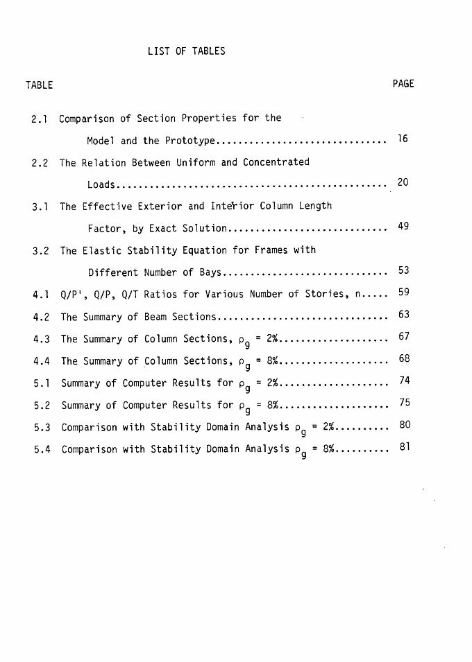
LIST OF TABLES

TABLE PAGE

2.1 Comparison of Section Properties for the

Model and the Prototype ..•............................ 16

2.2 The Relation Between Uniform and Concentrated

Loads.. . . . . . . . . . . . . . . . . . . . . . . . . . . . . . . . . . . . . . . . . . . . . . . . 20

3. 1 The Effective Exterior and Interior Column Length

Factor, by Exact Solution ..•.........................• 49

3.2 The Elastic Stability Equation for Frames with

Different Number of Bays .........••.....•............. 53

4. 1 Q/P', Q/P, Q/T Ratios for Various Number of Stories, n ..... 59

4.2 The Summary of Beam Sections ............................... 63

4.3 The Summary of Column Sections, Pg= 2% .................... 67

4.4 The Summary of .Column Sections, Pg= 8% .................... 68

5.1 Summary of Computer Results for Pg= 2% .•...............•.. 74

5.2 Summary of Computer Results for Pg= 8% ................•... 75

5.3 Comparison with Stability Domain Analysis Pg= 2% .••....... 80

5.4 Comparison with Stability Domain Analysis Pg= 8% .......... 81

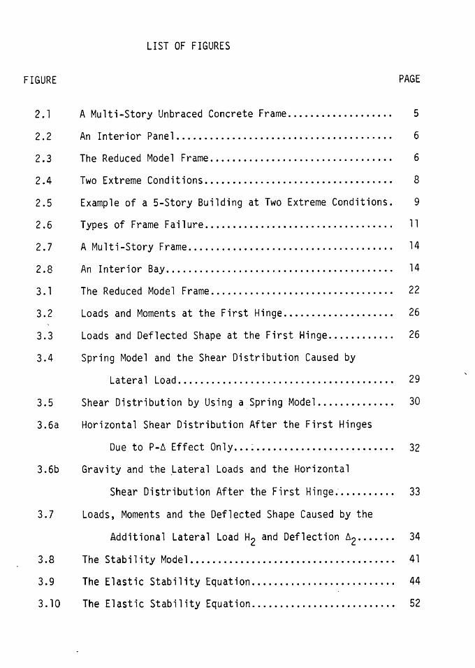
LIST OF FIGURES

FIGURE PAGE

2.1 A Multi-Story Unbraced Concrete Frame................... 5

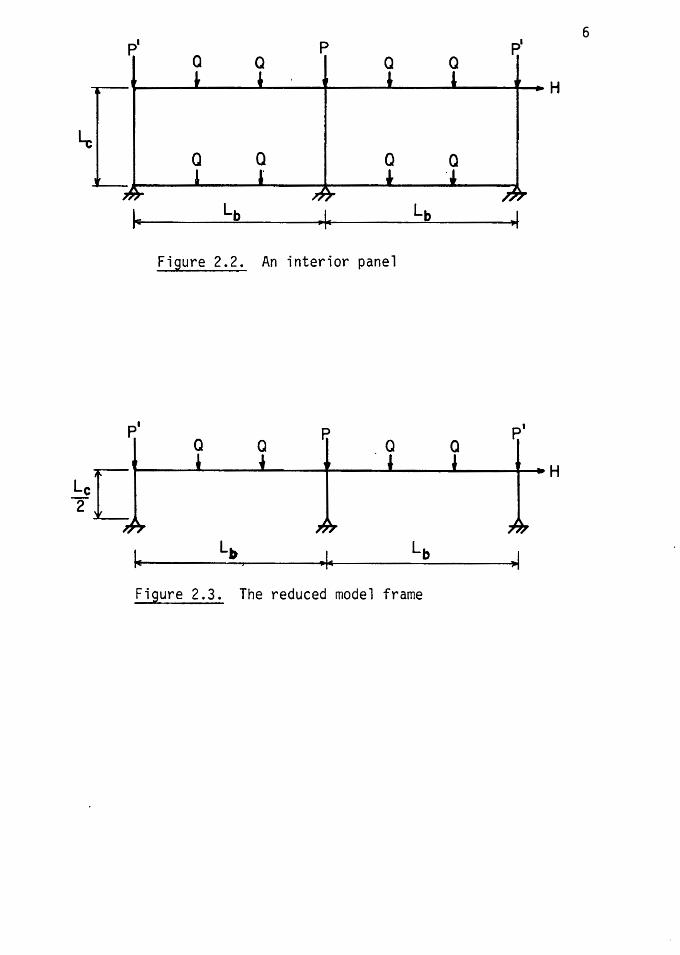
2.2 An Interior Panel....................................... 6

2.3 The Reduced Model Frame................................. 6

2.4 Two Extreme Conditions.................................. 8

2.5 Example of a 5-Story Building at Two Extreme Conditions. 9

2.6 Types of Frame Failure.................................. 11

2.7 A Multi-Story Frame..................................... 14

2.8 An Interior Bay......................................... 14

3.1 The Reduced Model Frame................................. 22

3. 2 Loads and Moments at the First Hinge......... . . . . . . . . . . . 26

3.3 Loads and Deflected Shape at the First Hinge............ 26

3.4 Spring Model and the Shear Distribution Caused by

Latera 1 Load. . . . . . . . . . . . . . . . . . . . . . . . . . . . . . . . . . . . . . . 29

3.5 Shear Distribution by Using a.Spring Model.............. 30

3.6a Horizontal Shear Distribution After the First Hinges

Due to P-~ Effect Only ... :......................... 32

3.6b Gravity and the ~ateral Loads and the Horizontal

Shear Distribution After the First Hinge;.......... 33

3.7 Loads, Moments and the Deflected Shape Caused by the

Additional Lateral Load H2 and Deflection ~2 ....... 34

3.8 The Stability Model ..................................... 41

3.9 The Elastic Stability Equation.......................... 44

3.10 The Elastic Stability Equation.......................... 52

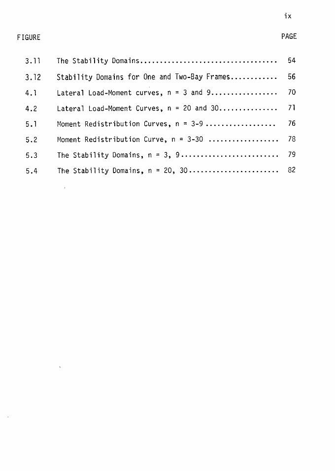
ix

FIGURE PAGE

3.11 The Stability Domains................................... 54

3.12 Stability Domains for One and Two-Bay Frames ............ 56

4.1 Lateral Load-Moment curves, n = 3 and 9................. 70

4.2 Lateral Load-Moment Curves, n = 20 and 30............... 71

5.1 Moment Redistribution Curves, n = 3-9..... .. . . . . . . . . . . . 76

5.2 Moment Redistribution Curve, n = 3-30 .................• 78

5.3 The Stability Domains, n = 3, 9 ......................... 79

5.4 The Stability Domains, n = 20, 30 ....................... 82

CHAPTER I

INTRODUCTION

1.1 GENERAL

The inelastic behavior of reinforced concrete structures has been

recognized for several decades (1,2), and the related research which

spans over half a century (3) have clarified a number of important pro­

blems. However, despite the fact that there are some available theore­

tical and experimental data, the adoption of inelasticity concept in

structural design of reinforced concrete remains elusive. Convention-'

ally, the analyses of indeterminate reinforced concrete structures has

been based on elastic method. The elastic method consists of determin-

ing the bending moments shear and axial thrusts by assuming that the

structure is perfectly elastic, i.e., the material's stress-strain

relationship varies linearly.

Since 1963, the American Concrete Institute (4), through the use

of Ultimate Strength Design (USO), has allowed designing individual

members and sections by recognizing their inelastic response, while the

elastic structure is assumed to determine the moments and forces. In

USO, the required strength to resist loads is found by multiplying the

service loads by load factors, corresponding to the type of loading

conditions. These load factors for a number of loading combinations

have been determined based on the probability of the combination occurr­

ing and on the safety of the structure. The USO method is also used by

codes of practice in several other countries such as Great Britain· and

the Soviet Union (5,6).

2

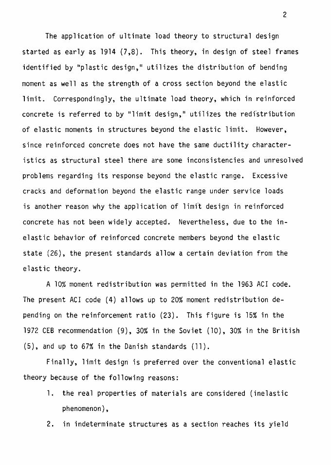
The application of ultimate load theory to structural design

started as early as 1914 (7,8). This theory, in design of steel frames

identified by 11 plastic design," utilizes the distribution of bending

moment as well as the strength of a cross section beyond the elastic

limit. Correspondingly, the ultimate load theory, which in reinforced

concrete is referred to by "limit design," utilizes the redfstribution

of elastic moments in structures beyond the elastic limit. However,

since reinforced concrete does not have the same ductility character­

istics as structural steel there are some inconsistencies and unresolved

problems regarding its response beyond the elastic range. Excessive

cracks and deformation beyond the elastic range under service loads

is another reason why the application of limit design in reinforced

concrete has not been widely accepted. Nevertheless, due to the in­

elastic behavior of reinforced concrete members beyond the elastic

state (26), the present standards allow a certain deviation from the

elastic theory.

A 10% moment redistribution was permitted in the 1963 ACI code.

The present ACI code (4) allows up to 20% moment redistribution de­

pending on the reinforcement ratio (23). This figure is 15% in the

1972 CEB recommendation (9), 30% in the Soviet (10), 30% in the British

(5), and up to 67% in the Danish standards (11).

Finally, limit design is preferred over the conventional elastic

theory because of the following reasons:

1. the real properties of materials are considered (inelastic

phenomenon),

2. in indeterminate structures as a section reaches its yield

3

point, the structure will not collapse,

3. the reserved strength, beyond the elastic point to failure,

is usually considerable, and

4. reduction of negative moments reduces the steel concentration.

1.2 OBJECTIVE

The general objective of this investigation is to determine the

applicability of limit design to multistory multibay unbraced concrete

frames. The primary objective is to study the behavior of such frames

under gravity and gravity plus lateral loading for the following con­

ditions:

(a) as the loading increases

(b) as the relative flexural stiffness of the columns and beams

varies

(c) as the beam to column load ratio increases

(d) as the reinforcement ratio varies

This investigation is carried out using two analytical techniques.

1.3 ORGANIZATION

The remaining part of this thesis is divided into five chapters.

In Chapter II, the modeling consideration is discussed. In Chapter III,

analytical treatment of frames using the mathematical solution of

an elasto-plastic stability model frame is discussed.

The computer analysis of these model frames, using a computer

program which takes material and geometry nonlinearities into account,

is discussed in Chapter IV. Chapter V discusses the comparison of the

two methods of analysis used for selected model frames, and finally

Chapter VI includes the summary and conclusions of this study, along

with some recommendations for future research.

CHAPTER II

MODELING CONSIDERATIONS

2. 1 GENERAL

ln this chapter, overall loading patterns, load relationships

with some simplifying assumptions, different types of frame failure,

and some general requirements of structural similitude will be discussed.

The purpose of this chapter is to set the background stage for the

analytical treatment which follows in Chapters III and IV.

2.2 THE MODEL OF UNBRACED FRAME

In designing a reinforced concrete building frame, several loading

patterns must be considered. A critical condition for frame in­

stability exists when all floors are fully loaded, thus creating

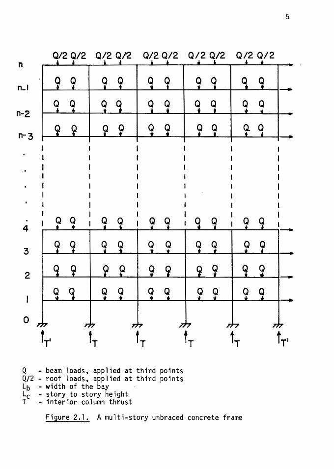
full axial loads in columns. An unbraced n-story concrete frame is shown

in Fig. 2.1. The width of each bay (beam length) and the story to

story height (column length) are Lb and Lc respectively. It is assumed

that the center to center distance between frames is also equal to Lb.

A two bay interior panel which represents a typical interior

panel is shown in Fig. 2.2. Due to symmetry of the frame points of

inflection are at column midheights and for simplicity a reduced model

as shown in Fig. 2.3 will be analyzed. According to Rad (12) for a

single panel the relationship between column load P (applied at top)

and beam load Q, neglecting the increased column load due to lateral

load, can be expressed as:

Q/P = 1/(2n-2) (2. 1)

5

Q/2 Q/2 Q/2 Q/2 Q/2 Q/2 Q/2 Q/2 Q/2 Q/2

I I

n

I Q Q

I Q Q

I : Q I Q Q I Q Q I: "-' ~ ~ ~ n-2. ~ ~ ~ ~ ~ ;

n-3 I • • I • I I • • I I: • I I • 1--.

Q Q Q Q Q Q Q 4 ,_ __ ..... ____ ._ ____ pm-__ ..... ____ ..._ ____ +-__ _. __________ ...,.. __ _. ____ ..... ____ ..... __ ..... ________ ..... ~

3 Q Q Q Q Q Q Q Q Q Q

2 .,.. __ .... ._ __ _....._ ____ ,.... __________ .... ____ ...., __________ .._ ____ .,. ____ ...,~ __ ..... ____ ....,~--------.-.----.... --..

Q Q Q Q Q Q Q Q Q I - • I • • I • r I T Y I I • 1--..

0

fT, f T f T

Q - beam loads, applied at third points Q/2 - roof loads, applied at third points Lb - width of the bay Le - story to story height T - interior column thrust

f T f T

Figure 2.1. A multi-story unbraced concrete frame

h·

9

awEJJ lapow pa~npaJ a41

,.,. 41 1

H--+----------------+--~------~--~J~

0 0 0 0 d

7

And the relationship between the column thrust T and the beam load Q as:

Q/T = l/(2n-l) (2.2)

where n = number of stories. Considering the reduced model shown in

Fig. 2.3, equation 2.1 is not valid for 2-bay frame, however, it will

be shown later that Equation 2.2 is still true. For a 2-bay frame,

the applied column loads P and P' must be chosen such that the column

thrusts T are all the same. For the exterior and interior column loads

P' and P at the first floor, the corresponding equations become:

Q/P' = l/(2n-2); and

Q/P = l/(2n-3)

(2.3)

(2.4)

Equation 2.2 will remain unchanged. Again, for Equation 2.3 and 2.4

the increased column load ~aused by the lateral load H is neglected.

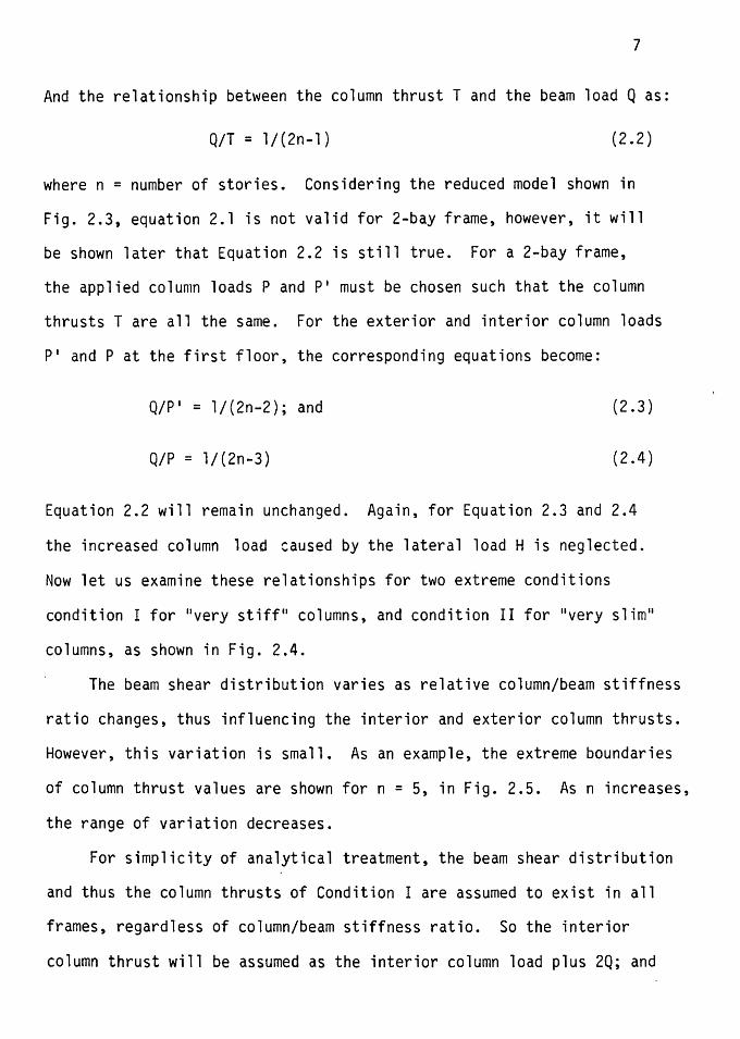
Now let us examine these relationships for two extreme conditions

condition I for "very stiff 11 columns, and condition II for "very slim"

columns, as shown in Fig. 2.4.

The beam shear distribution varies as relative column/beam stiffness

ratio changes, thus influencing the interior and exterior column thrusts.

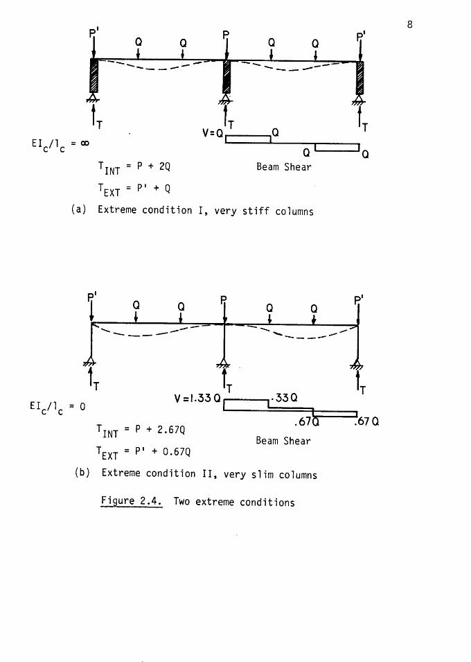
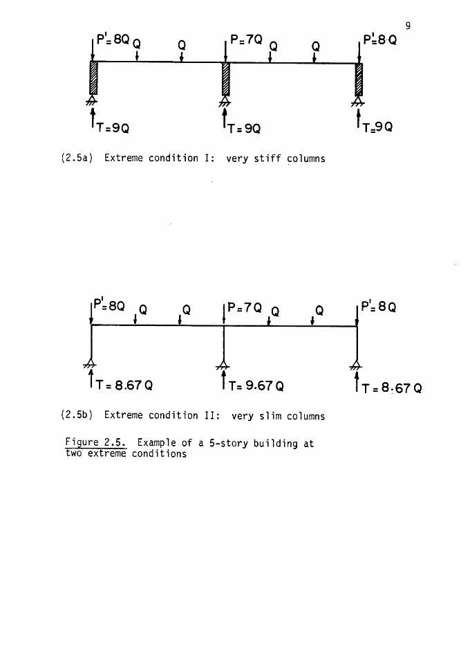
However, this variation is small. As an example, the extreme boundaries

of column thrust values are shown for n = 5, in Fig. 2.5. As n increases,

the range of variation decreases.

For simplicity of analytical treatment, the beam shear distribution

and thus the column thrusts of Condition I are assumed to exist in all

frames, regardless of column/beam stiffness ratio. So the interior

column thrust will be assumed as the interior column load plus 2Q; and

P.' a a P. a a P.'

-- ................... _ - ---- ---

f T fr a 'T V=Q I EI /1 = ex> I

a' 'a c c

TINT = p + 2Q Beam Shear

TEXT = P' + Q

(a) Extreme condition I, very stiff columns

a a P. a a P.'

1T Eic/lc = 0

TINT = P + 2.67Q

TEXT = P' + 0.67Q

I r33Q

.67h .'67 a Beam Shear

(b) Extreme condition II, very slim columns

Figure 2.4. Two extreme conditions

8

P1:8Q Q

J

tT:9Q

a P:7Q Q Q

'T=9Q

(2.5a) Extreme condition I: very stiff ~olumns

I t=BQ 1a Q

l T = 8.67Q

ip= 7Q Q

f T= 9~67Q

Q I

(2.5b) Extreme condition II: very slim columns

Figure 2.5. Example of a 5-story building at two extreme conditions

9 P~S·Q

tT:9Q

P1:8Q

f T=8~67Q

10

the exterior column thrust as the exterior column load plus Q.

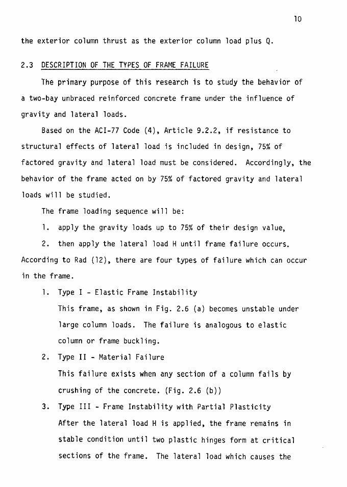
2.3 DESCRIPTION OF THE TYPES OF FRAME FAILURE

The primary purpose of this research is to study the behavior of

a two-bay unbraced reinforced concrete frame under the influence of

gravity and lateral loads.

Based on the ACI-77 Code (4), Article 9.2.2, if resistance to

structural effects of lateral load is included in design, 75% of

factored gravity and lateral load must be considered. Accordingly, the

behavior of the frame acted on by 75% of factored gravity and lateral

loads will be studied.

The frame loading sequence will be:

1. apply the gravity loads up to 75% of their design value,

2. then apply the lateral load H until frame failure occurs.

According to Rad (12), there are four types of failure which can occur

in the frame.

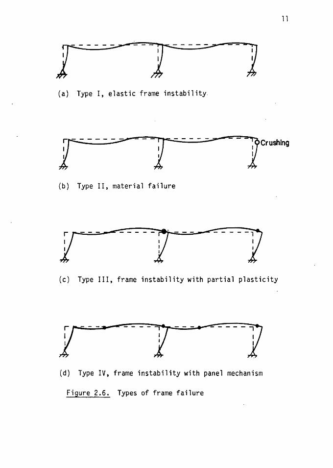
1. Type I - Elastic Frame Instability

This frame, as shown in Fig. 2.6 (a) becomes unstable under

large column loads. The failure is analogous to elastic

column or frame buckling.

2. Type II - Material Failure

This failure exists when any section of a column fails by

crushing of the concrete. (Fig. 2.6 (b))

3. Type III - Frame Instability with Partial Plasticity

After the lateral load H is applied, the frame remains in

stable condition until two plastic hinges form at critical

sections of the frame. The lateral load which causes the

1l

r----=----·r---~ 1 (a) Type I, elastic frame instability.

r---:;..;:>"'"" y-----~ --1Crushir

(b) Type II, material failure

y---- --~7

(c) Type III, frame instability with partial plasticity

r (d) Type IV, frame instability with panel mechanism

Figure 2.6. Types of frame failure

12

first set of plastic hinge to form is designated by H1. In

this type of failure, due to the loss of frame stiffness after

the first hinges, the frame can no longer stay in stable equi-

1 ibrium position. (Fig. 2.6 (c))

4. Type IV - Frame Instability with Development of a Panel

Mechanism

The frame will stay in a stable equilibrium until enough

plastic hinges form in the frame to produce an, unstable mech­

anism. The extra lateral load beyond H1 that is necessary

to produce a mechanism is designated by H2. (Fig. 2.6 {d))

In this present study, we will not focus on Types I and II failure,

but the boundary between Types III and IV failure will be examined.

The lateral load terminology will be as follows:

H = H1 + H2

where: H = Total lateral load which is resisted by the frame

H1 = Lateral load to produce the first set of two plastic hinges

H2 = Lateral load in excess of H1 to produce the panel mech­

anism

Also, a useful index can be introduced as the percentage of moment

redistribution, defined as s,

S = (H2/H){l00) (2.5)

for Type III failure:

H2 = 0, S = 0, and H = H1

13

for Type IV failure:

H2 > 0, S > 0, and H = H1 + H2

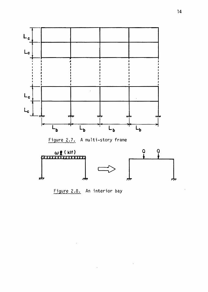
2.4 LOADING OF THE PROTOTYPE VS. MODEL FRAMES

In this section an interior bay of a multistory structure will be

considered (Fig. 2.7) and the loading relationship between the proto­

type and the model with regard to scale factor (SF), structural analysis,

and member strength will be determined.

2.4.l Frame Loading. Considering Fig. 2.8, one may write:

Total beam load = (w£)Lb = 2Q, and

Column thrust, T = (w£)Lb for each floor

where: w = uniform load per unit area

~ = bent spacing

As discussed before:

Q/T = 1/2n-1-

or 2Q/2T = l/2n-1

or (w~)Lb/2T = l/2n-1

(2.2)

(2.6)

Equation 2.6 establishes the relationship between column thrust T

and number of stories n for a uniform surface load w.

2.4.2 Column Strength. In this section, the relation between the

column axial capacities of the model and the prototype is determined.

I

Pno = pure axial load capacity= 0.85 f c Ac+ (pA9)f Y

I

Le I

Le

Le

~

Lb

I

• I I I I I I r I

Lb Lb

Figure 2.7. A multi-story frame

wt. (kif)

I"llflOB*"l c::::>

Figure 2.8. An interior bay

14

Lb

a a

15

I

p 0.85 f c (A9 - Pm A ) + (p A )f no(m) _ m 9m m 9m Y

pno(p) - 0.85 f~ (Ag - pp A ) + (pp A )fy m 9p 9p

(2. 7)

where 11 m11 and 11 p11 refer to model and prototype respectively. The

comparison of the section properties between prototype and the model

is summarized in Table 2. 1.

By substituting for A9P in terms of A9m in Equation 2.7, the

following is obtained:

p Ag [ 0 .85 < ( 1-p) + pfy J no(m) _ m

p no ( p) - -( 1-/-SF_)...,,...2 _A __ [ 0-.-8~5 -f-1 -(-1--p-) _+_p_f_.1 gm c ~

or P = (l/SF) 2 (P ) no(p) no(m) (2.8)

For example, for a scale factor of 1/3, we get:

Pno(p) = gpno(m)

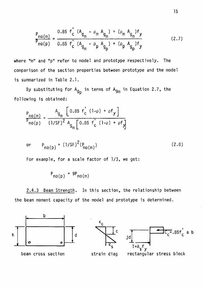
2.4.3 Beam Strength. In this section, the relationship between

the beam moment capacity of the model and prototype is determined.

,. b ., e:c

I hI 0 OJd ~=re jC ~ T=Af

c=.85f c a b

s y beam cross section strain diag rectangular stress block

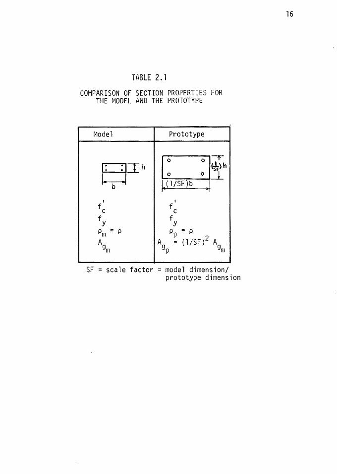
TABLE 2.1

COMPARISON OF SECTION PROPERTIES FOR THE MODEL AND THE PROTOTYPE

Model Prototype

:IIh I : 0 l~h I: 1. .f 0 ~

~(l/SF)b ~I b

I I

f c f c f f y y Pm = p p = p p A A = (l/SF) 2 A

gm gp gm

SF = scale factor = model dimension/ prototype dimension

16

1

I

if M = A5

f Y (jd), and p = As/bd

Mm = A5 f j dm m y

and MP = A f j d Sp y p

Mp/M = A5

fy j dp/A5

f j d m p m y m

or Mp_~ (l/SF * bm)(l/SF * dm)J fy (j) (l/SF * dm) Mm - [P ( bm )( dm) J f y ( j ) ( dm)

or M = (l/SF) 3 (M ) p m

For example, for a scale factor of 1/3, we get:

Mp = 27 (Mm)

17

(2.9)

2.4.4 The Structural Analysis. In this section, the structural

analysis with regard to the column axial thrust and beam moment will

be considered. Let us consider column load first.

pp = (wpR-p)Lbp and P = (w o. ) Lb m nrm m

Pp/Pm = (wp~p)Lb /(wm~m)Lb p m

or (l/SF)2 R-m Lb l

~ = (wp/wm)[ R- Lb m] m m m

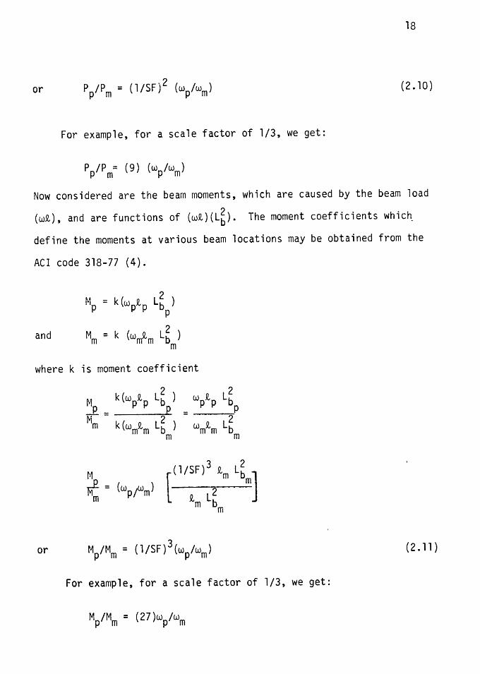
18

or - 2 Pp/Pm - (l/SF) (wp/wm) (2.10)

For example, for a scale factor of 1/3, we get:

Pp/Pm= (9) (wp/wm)

Now considered are the beam moments, which are caused by the beam load

(w£), and are functions of (w£)(L~). The moment coefficients whic~

define the moments at various beam locations may be obtained from the

ACI code 318-77 (4).

2 Mp = k (w p£ p Lb )

p

and Mm = k (wm£m L~ ) m

where k is moment coefficient

2 2 M k(wp£p Lb ) wp£p Lb Mp = 2p = 2p m k (wm£m Lb ) wm£m Lb

m m

(l/SF)3

£m L~ ] M m Ft-= (wp/ilm) [ ~ L2

m m bm

or Mp/Mm = (1/SF) 3(wp/wm)

For example, for a scale factor of 1/3, we get:

Mp/Mm = (27)wp/wm

(2.11)

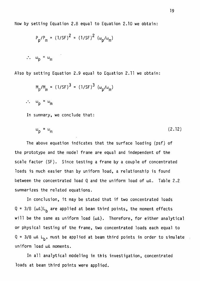
19

Now by setting Equation 2.8 equa1 to Equation 2.10 we obtain:

Pp/Pm= (1/SF) 2 = (l/SF) 2 (wp/wm)

wp = wm

Also by setting Equation 2.9 equal to Equation 2. 11 we obtain:

M /M = (l/SF) 3 = (l/SF) 3 (w /w ) p m p m

wp = wm

In summary, we conclude that:

w = w P m (2.12)

The above equation indicates that the surface loading (psf) of

the prototype and the model frame are equal and independent of the

scale factor (SF). Since testing a frame by a couple of concentrated

loads is much easier than by uniform load, a relationship is found

between the concentrated load Q and the uniform load of wi. Table 2.2

summarizes the related equations.

In conclusion, it may be stated that if two concentrated loads

Q = 3/8 (w1)Lb are applied at beam third points, the moment effects

will be the same as uniform load (w1). Therefore, for either analytical

or physical testing of the frame, two concentrated loads each equal to

Q = 3/8 w1 Lb' must be applied at beam third points in order to simulate

uniform load wi moments.

In all analytical modeling in this investigation, concentrated

loads at beam third points were applied.

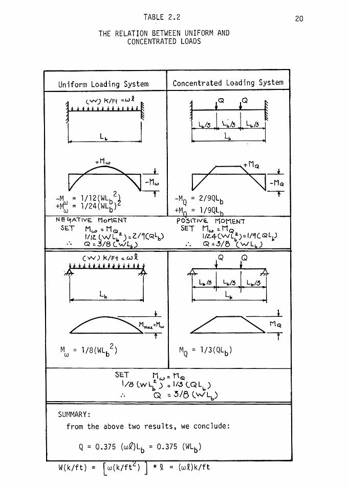
1 TABLE 2.2

THE RELATION BETWEEN UNIFORM AND CONCENTRATED LOADS

Uniform Loading System Concentrated Loading System

~ <. -H) k/ff ~wR !HH!HHHH~

I. L. J

-t-M(A,)

~ _!_ v '\J-M~ -Mw = l/12(WL 2) ----r +Mw = l/24(WL~)2 NE C;AilVE. MoM~NT

SET Mc..:>= MQ l//Z. lWL1:,z) = Z/1(Qlb)

· • Q :3/8 LwLb)

( vv) k/Fi :. w ~ ,kt tJ it H ft H t HJ

I Lb I • •

1 iQ ,a ~

L.ls l L~f.5 J, Lb/.5

-MQ = 2/9Qlb +Mn = l/9QLh

L,,

P05\"TIVE. MOMENI SEI Mw =- MQ

l/Z.4(VVL:)= 1/'i(G2LJ . . Q =-3/B (WL6 )

.Q 'Q ~ L" /.5 J Lb/.5 J Lb/.5 .,lit.

-..-'I

LP

+ ~--~~ -,-

l

L s-;: MW= l/8(WLb2) MQ = l/3(QLb)

SE.T M(,..J = nQ \/a (wl:) =-II~ (QL'=) :. Q :. 3/5 (WLb)

SUMMARY: from the above two results, we conclude:

Q = 0.375 (wQ)Lb = 0.375 (WLb)

W(k/ft) = [ w(k/ft~) ] * ~ = (w~)k/ft

20

3.1 GENERAL

CHAPTER III

ELASTO-PLASTIC MODEL

The stability of unbraced frames using an analytical method will be

discussed in this chapter. This method consists of the mathematical

solution of an elasto-plastic stability model. This solution will define

the boundaries where limit design may be feasible.

In this stability analysis, the reduced model of Fig. 3.1 is investi­

gated. The behavior of the model frame as acted upon by column loads,

beam loads, and lateral force is studied. The stability equation of the

frame, when frame becomes unstable is determined by the principle of

neutral equilibrium. The stability equation is also determined by Bolton's

{15) method.

The stability equation of the frame when it becomes unstable under

the action of gravity loads alone without lateral load is also determined.

3.2 FRAME LOADING, ASSUMPTIONS, AND NOTATION

The loading sequence for this model frame is in accordance with ACI

318-77, Art. 9.2.2, as discussed in Sec. 2.3. Axial column loads P and

beam loads Q are first applied proprotionally up to 75% of the predicted

ultimate capacity of the frame. Next, lateral load H is applied until total

failure of the frame is reached. The lateral deflection of the model is

half that of the actual frame.

In the stability analysis of the model, the following assumptions (12)

are made:

1. The beam members and column members possess an elasto-plastic

3 1

d 0 d

22

23

moment-curvature (M-~) relationship. Also, the flexural

rigidities of the column (Elc) and the beam (Eib) do not vary

along the length of the members.

2. The change in the magnitude of column thrust caused by the

lateral force H, is neglected.

3. The change in moment due to the product of column axial thrust

and the column deflection from the chord connecting the column

ends is neglected, i.e., the moment diagram is triangular.

4. The beam bending moment capacity, MP, for the negative and

positive bending is the same.

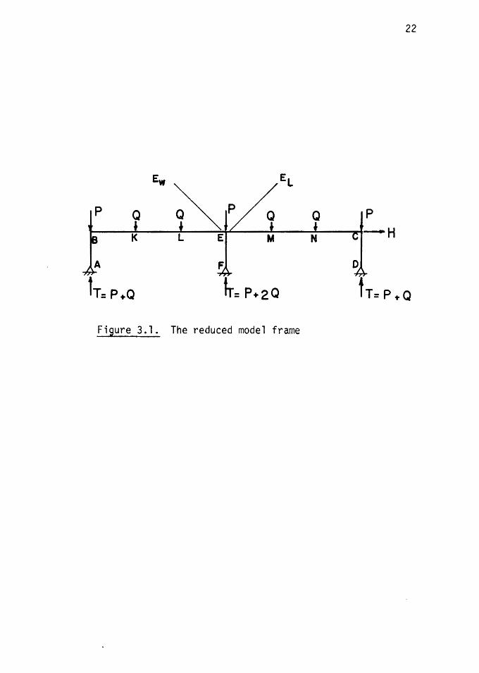
The reduced model frame of Fig. 2.3 is used for analysis with the

difference that, for simplicity, all column axial loads are assumed to

be equal to Pas shown in Fig. 3.1. This frame is examined at two stages

of loading:

1. The first stage exists until the first hinges are developed at

corner C and section Ew due to gravity loads P, Q, and the

horizontal load H1.

2. The second stage exists after plastic hinges form at point k

and M due to the additional horizontal force H2.

The definitions of symbols used in the following discussion are

given below:

P axial load on the column

Q applied load on the beam third points

Lb length of the beam

Lc length of the column

MP plastic moment capacity of the beam (or column)

Elb flexural stiffness of the beam

Eic flexural stiffness of the column

w relative flexural stiffness of the column and beam

EI/Le = Eib/Lb

H lateral load applied at corner C

24

H1 lateral load required for the formation of the first hinges

in the frame (at corner C and Ew)

H2 additional lateral load required for the formation of the

second hinges in the frame (at k and M)

~ horizontal deflection of the frame

~l horizontal deflection of the frame at the formation of first

hinges

~2 additional horizontal deflection of the frame at the formation

of second hinges.

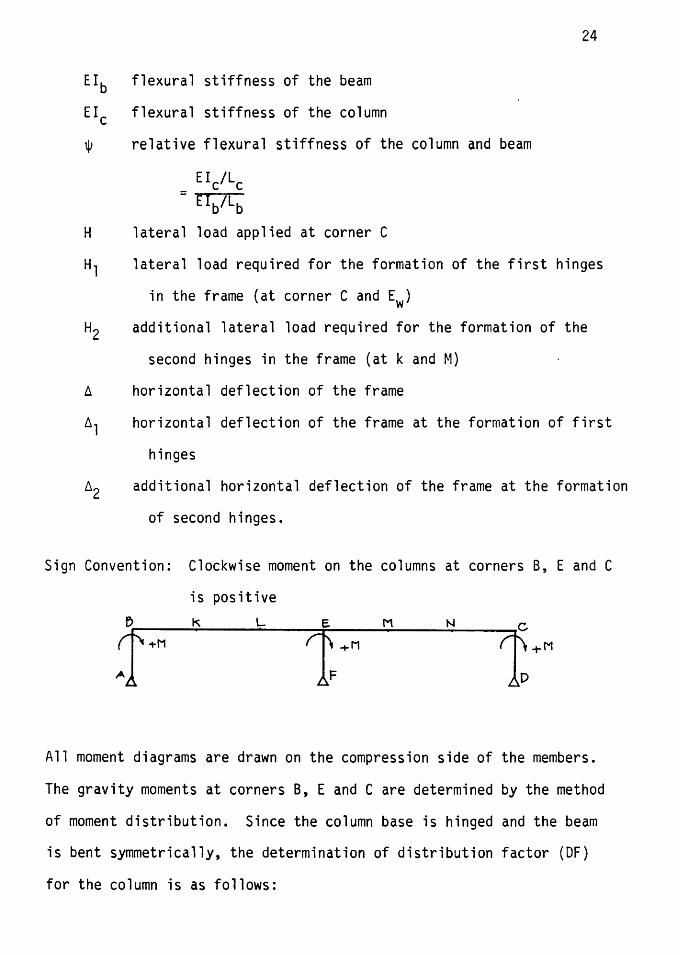
Sign Convention: Clockwise moment on the columns at corners B, E and C

is positive J +M k L 1F +M M N t +M

All moment diagrams are drawn on the compression side of the members.

The gravity moments at corners B, E and C are determined by the method

of moment distribution. Since the column base is hinged and the beam

is bent symmetrically, the determination of distribution factor (OF)

for the column is as follows:

25

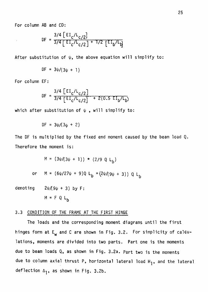
For column AB and CD:

3/4 [ Elc/Lc/2] DF = 3/4 [ Ef c/Lc/2] + l/2 [ E Ib/L~

After substitution of w, the above equation will simplify to:

oF = 3wl( 3w + 1 )

For column EF:

3/4 [ Elc/Lc/2 J OF = 3/4 [Eic/Lc/2] + 2(0.5 Elb/lb)

which after substitution of w , will simplify to:

oF = 3w/(3w + 2)

The OF is multiplied by the fixed end moment caused by the beam load Q.

Therefore the moment is:

M = ( 3w I( 3w + 1 ) ) * ( 2 I 9 Q Lb )

or M = (6w/27W + 9)Q Lb = (2w/(91'J + 3)) Q Lb

denoting 2wA9w + 3) by F:

M = F Q Lb

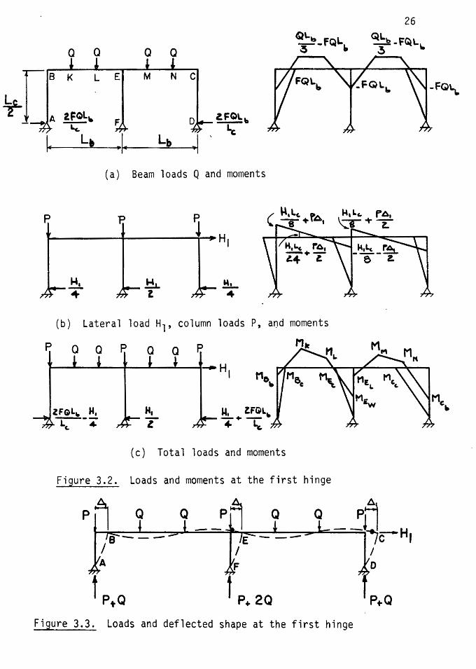
3.3 CONDITION OF THE FRAME AT THE FIRST HINGE

The loads and the corresponding moment diagrams until the first

hinges form at E and C are shown in Fig. 3.2. For simplicity of calcu-w

lations, moments are divided into two parts. Part one is the moments

due to beam loads Q, as shown in Fig. 3.2a. Part two is the moments

due to column axial thrust P, horizontal lateral load H1, and the lateral

deflection~,, as shown in Fig. 3.2b.

118 -'f-L.JA 2FQL"

- Le.

1, Ltt

p

M, ...

F D ~ .. ~

(a) Beam loads Q and moments

P.

M, l

~ H1

.!h.. 4

(b) Lateral load H1, column loads P, and moments

1aa1aa1 l J l i .....-H I

M. ZFGL'-- + -... '-c.

(c) Total loads and moments

Figure 3.2. Loads and moments at the first hinge

A Q Q Pil Q Q -~LI

E---- ljCHI I I

A ! ,o

t PtQ t P+ 2Q f P+Q

Figure 3.3. Loads and deflected shape at the first hinge

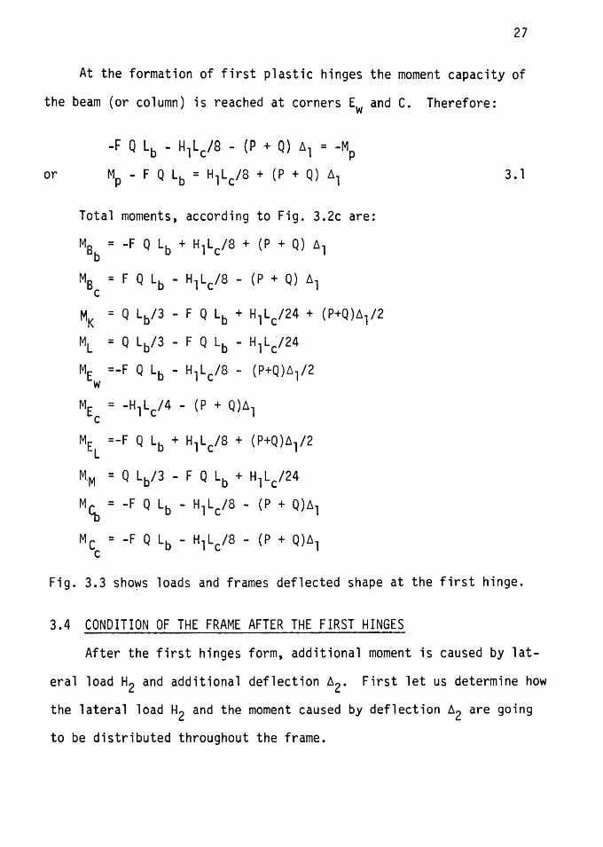
27

At the formation of first plastic hinges the moment capacity of

the beam (or column) is reached at corners Ew and C. Therefore:

or

-F Q Lb - H1Lc/S - (P + Q) Al = -MP

Mp - F Q Lb = H1Lc/8 + (P + Q) Al

Total moments, according to Fig. 3.2c are:

M8b = -F Q Lb + HlLc/8 + (P + Q) ~l

M8 = F Q Lb - H1Lc/8 - (P + Q) ~l c

MK = Q Lb/3 - F Q Lb + H1Lc/24 + (P+Q)~ 1 /2

ML = Q Lb/3 - F Q Lb - H 1 L~/24

ME =-F Q Lb - H1Lc/8 - (P+Q)~ 1 /2 w ME = -H1Lc/4 - (P + Q)~l

c

MEL =-F Q Lb + H1Lc/8 + (P+Q)Al/2

MM = Q Lb/3 - F Q Lb + H1Lc/24

MCb = -F Q Lb - HlLc/8 - (P + Q)Al

Mc = -F Q Lb - H1L /8 - (P + Q)Al c c

3. 1

Fig. 3.3 sho~s loads and frames deflected shape at the first hinge.

3.4 CONDITION OF THE FRAME AFTER THE FIRST HINGES

After the first hinges form, additional moment is caused by lat­

eral load H2 and additional deflection A2• First let us determine how

the lateral load H2 and the moment caused by deflection A2 are going

to be distributed throughout the frame.

28

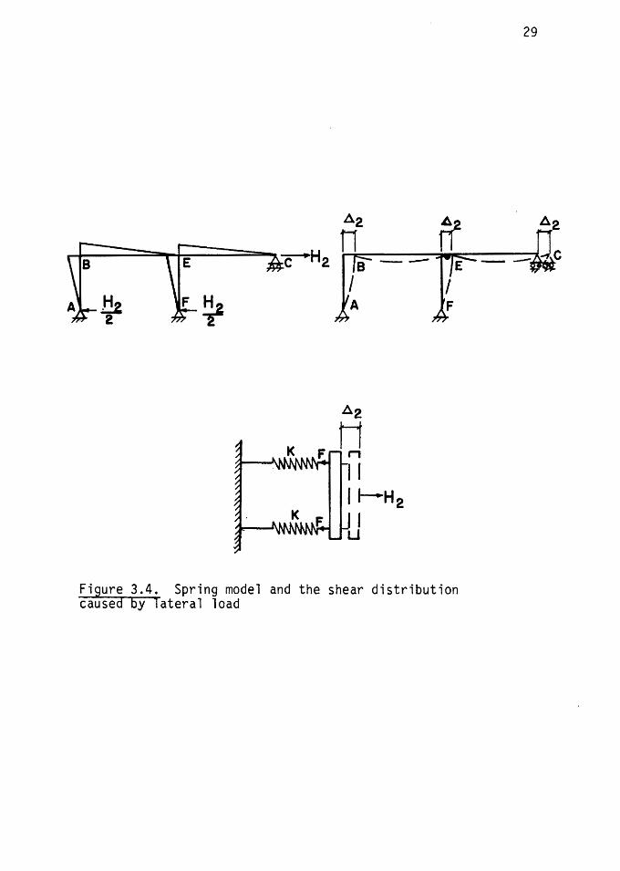
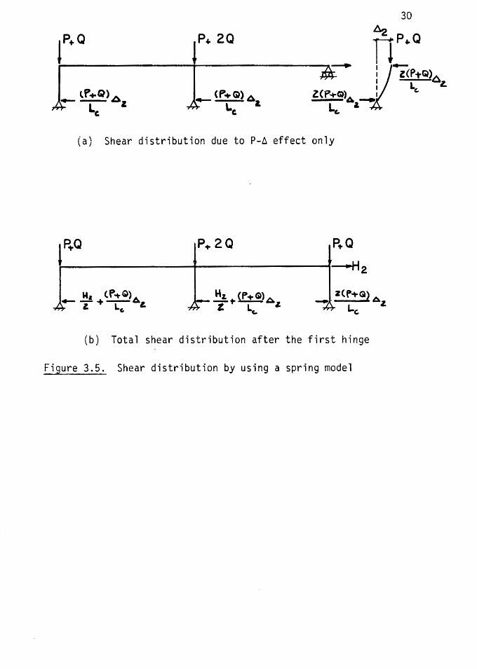
3.4.1 Shear Distribution by Using a Spring Model. Let us consider

the (~ 2 ) effect only which is caused by lateral force H2. Since moment

at joint C has reached its capacity Mp, the model can be reduced to what

is shown in Fig. 3.4. This reduced model can be further simplified to

a set of springs having a stiffness of k. As the tensile force H2 is

applied, both springs will be stretched the same amount of ~ 2 . The

tensile force in each spring will be equal to H212. Therefore by this

reasoning the horizontal shear distribution at the column supports of A

and F due to lateral force H2 will be equal to H212.

As the frame deflects, the moment at corner Ew and C must remain

constant at moment capacity, MP. Therefore the added moment, (P+Q)~ 2 ,

on the column CD must be opposed by a horizontal shear force equal to

2(P+Q)~ 2/Lc. This shear force is transferred to column EF and AB such

as to keep the frame in equilibrium.

Again by considering the spring model shown in Fig. 3.4 and the

analogy explained above, this shear force must be distributed equally

at the column supports A and F, as shown in Fig. 3.Sa.

By combining the P-~ 2 and the lateral load H2 effects, the shear

distribution as shown in Fig. 3.Sb is obtained.

3.4.2 Shear Distribution by Yura's ,Method. A second technique

presented by Yura (13) may be used to determine the horizontal shear

distribution at the supports of A, F and D.

In general, the total gravity load which produces sidesway can be

distributed among the columns in a story in any manner. Sidesway will

not occur until the total frame load on a story reaches the sum of the

potential individual column loads for the unbraced frame. In our model

~

~H2 c --

A2

Ii n ·1 I

I ,_..H2 I u

Figure 3.4. Spring model and the shear distribution caused by lateral load

29

l 1

(•Q P.a. 2Q

lf+Q) A ..--~,

LC <P+Gl) 61.

~ L. c

(a) Shear distribution due to P-~ effect only

lP+Q

Ma <.P""t Q) A .... -+--.a&. Z L,

P+ 2Q

Hz. (P+&)Az -to L z c.

(b) Total shear distribution after the first hinge

Figure 3.5. Shear distribution by using a spring model

30

31

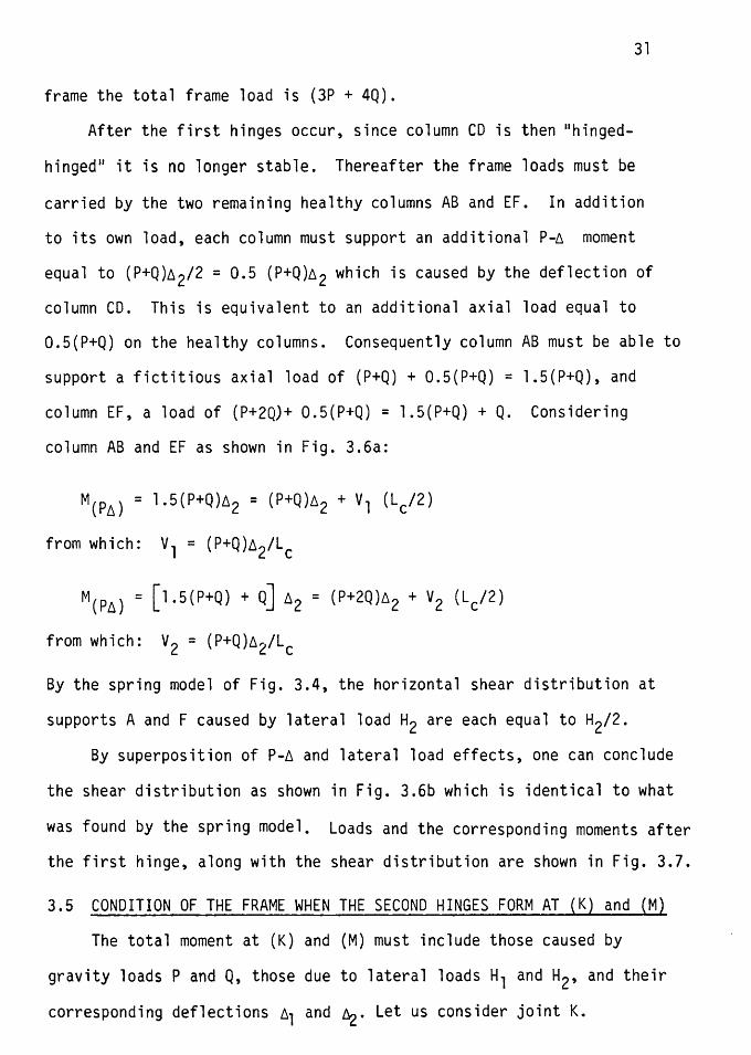
frame the total frame load is (3P + 4Q).

After the first hinges occur, since column CD is then "hinged­

hinged" it is no longer stable. Thereafter the frame loads must be

carried by the two remaining healthy columns AB and EF. In addition

to its own load, each column must support an additional P-6 moment

equal to (P+Q)6 2/2 = 0.5 (P+Q)6 2 which is caused by the deflection of

column CD. This is equivalent to an additional axial load equal to

O.S(P+Q) on the healthy columns. Consequently column AB must be able to

support a fictitious axial load of (P+Q) + 0.5(P+Q) = l.5(P+Q), and

column EF, a load of (P+2Q)+ 0.5(P+Q) = l.5(P+Q) + Q. Considering

column AB and EF as shown in Fig. 3.6a:

M(P6) = l.5(P+Q)62 = (P+Q)62 + v1 (Lc/2)

from which: v1 = (P+Q)A2/Lc

M(PA) = [1.5(P+Q) + Q] 62 = (P+2Q)62 + v2 (Lc/2)

from which: v2 = (P+Q)62/Lc

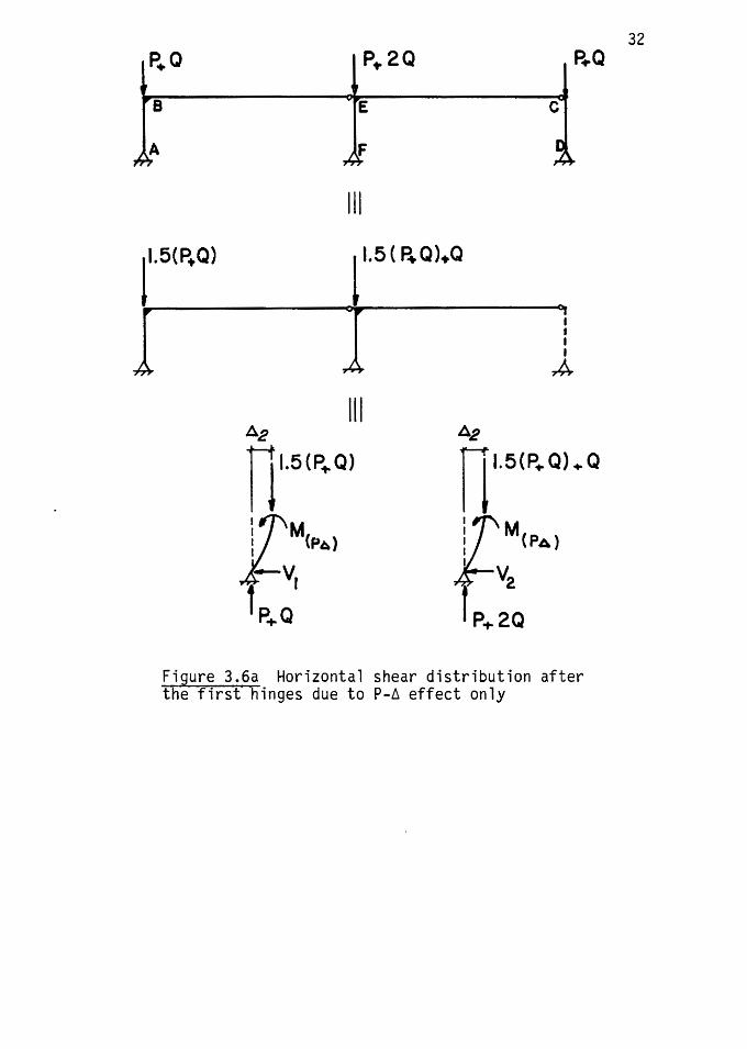
By the spring model of Fig. 3.4, the horizontal shear distribution at

supports A and F caused by lateral load H2 are each equal to H2/2.

By superposition of P-A and lateral load effects, one can conclude

the shear distribution as shown in Fig. 3.6b which is identical to what

was found by the spring model. Loads and the corresponding moments after

the first hinge, along with the shear distribution are shown in Fig. 3.7.

3.5 CONDITION OF THE FRAME WHEN THE SECOND HINGES FORM AT (K) and (M)

The total moment at (K) and (M) must include those caused by

gravity loads P and Q, those due to lateral loads H1 and H2, and their

corresponding deflections 61 and ~· Let us consider joint K.

P.Q

B

(5(P+Q)

l

P+2Q P,..Q

E

F

111

1"5 ( P+O)+Q

°I

I 111

'12

nl.5(P+Ql

i M (PA)

v r f P+Q

I

• • I

A

A2

nl.5(P+Q).Q

i.M (PA)

V, 2

r P+2Q

Figure 3.6a Horizontal shear distribution after the first hinges due to P-~ effect only

32

P+O

~

nl.5(P.Q)

¥8

A <l' ... Q) A. --- --~ t Le P+Q

A2 n 1.5( eQ).Q

JLE

F .-- <P~) Az. L,

lP'i-2 Q

Due to P-~ effect only

+

J_ ~2 El H2 vl--2

Due to lateral and H2, only

111

33

r+ 2Q r~Q

__., H2

.,._ (P .... Q) 4 -t M& L 2 2. c:.

. .- ~z crTCal)Az. + 2 L

' Z(P+Q)A.z

'-t.

Figure 3.6b. Gravity and the lateral loads, and the horizontal-shear distribution after the first hinge

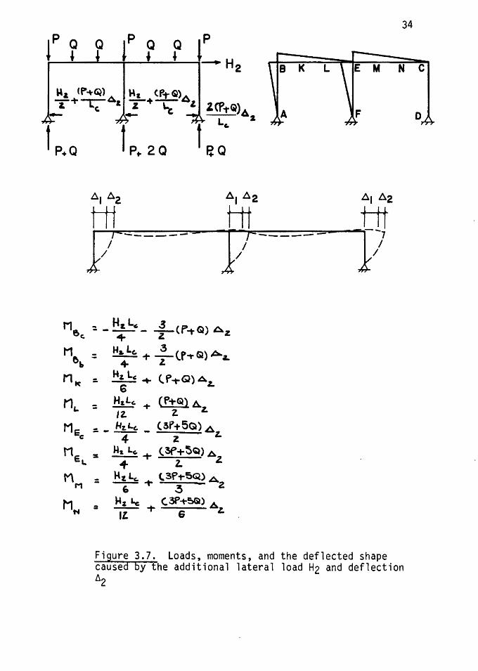
34

(? ? ( Q

p

---+H2 L

M~ (Po+~) Al~' <P...-&)A z:--t--rz- & z+\:t -zl Z(f1"Q)A r..,_ 4- ~ L s ~ t ' t P+ Q t P .. 2 Q P. Q

Al ~2 Al A2 A1 .6.2

Hi Hi tit l/'----- - I/r------ J? M ... H&L~ .3 CP. I!!>------ ;-G)Az.

c. + z M~ : Ha. Le. + 2-_ (f ;- Q) Az..

~ + z. n ec :. Hz. Le: + <. P"1-Q) Az.

6 M : H&L, + (P+Gl) A

&. 12. z. z. Me :. _ kz.L.c. _ (aP+5Q) .6,_

c 4 z M - M1 Le. + (3P+5Q) A

eL - T z. z. n _ H~L, <.3f'..-SQ) A

M - ~T 3 2

M ~% Le (.3P+5Gi) A ...,=IL-t- 6 L

Figure 3.7. Loads, moments, and the deflected shape caused by the additional lateral load H2 and deflection ~2

35

The moment caused by gravity loads P and Q, lateral load H1 and its

respective deflection A1, is:

MK = Q Lb/3 - F Q Lb + Hl Lc/24 + (P+Q)~l/2 3.2

The moment caused by lateral load H2 and its respective deflection A2,

is:

MK = H2 Lc/6 + (P+Q)A 2 3.3

Therefore the total moment at K is found by addition of equations 3.2

and 3.3. Since at collapse this total is equal to MP:

Mp = [o Lb/3 - F Q Lb + Hilc/24 + (P+Q)A,/2

[H2Lc/6 + (P+Q)A 2]

which after simplifying ~nd rearranging gives:

H2Lc/2 = 3Mp - Q Lb + 3F Q Lb + [-H1L/8 - (P+Q)Al] -

[(P+Q)A 1/2] - 3(P+Q)A2 3.4

Now substitute for the value of [H1Lc/8 + (P+Q)6 1] and [(P+Q)6 1;2J

from equation 3.1 into equation 3.4:

or

H2Lc/2 = 3Mp - Q Lb + 3 F Q Lb - Mp + F Q Lb - Mp/2 ~ FQLb/2 +

Hllc/16 - 3(P+Q)A2

H2Lc/2 = 1.5 Mp - Q Lb+ 4.5 ~QLb + Hllc/16 - 3(P+Q)A2 3.5

The lateral load H2 and the lateral deflection A2 can be related by

applying the moment-area theorem to the triangular moment diagram

shown in Fig. 3.7. It has been shown, that for single story, single

36

bay frame ( 12 ) :

~ 2 = M Lb Lc/6 Eib + M Lc2/12 Eic

But considering the model of the frame after the first hinge, shown

in Fig. 3.4, the deflection equation relating ~2 to moment for single

story-two bay frame is one-half as much. Therefore

~ 2 = M Lb Lc/ ll Elb + M Lc2/24 Elc 3.6

This is true since by addition of one bay we have doubled the stiffness •

of the structure. Therefore the deflection due to lateral load is only

one-half. From Fig. 3.7:

M = H2 Lc/4 + 3/2 (P+Q)~2

Therefore:

fH 2 L c + ~ ( P+Q ) ll 2 J Lb L c + ~ _l £4~~~--=~~

2 - 12 Elb

But since Elc/Lc

1V = Elb/Lb

fH2 LC + ~ (P+Q)t.2 J Lc 2 t 4 z 24 Elc

The above equation can be simplified and rearranged to:

(H2 L/ )(2w + 1)

~2 = 96 EIC/Lc - 6 LC (P+Q)(2w + 1)

Now by substitution of equation 3.8 into equation 3.5:

= Hl Le

1.5 Mp - Q Lb+ 4.S·F Q Lb+ 1 ~ - 3(P+Q)

(H2 Lc2)(2w + 1) [Y6 EI_/[_ - 6 L_ (P+0)(2w + l)J

3.7

3.8

37

or after simplifying and solving for H2, gives:

1 H l L c ( P+Q ) L / ( 2'11 + 1 ) H

2 = [ ( 1. 5 Mp - Q Lb + 4 • 5 F Q Lb + """"T6) [ 2 - g EI ]

c c

Now, the index value for the critical buckling load, defined as

2 TI EIC

PE = 2

may be substituted into the above equation. LC

1 H L 2 H2 = C ( 1. 5 Mp - Q Lb + 4. 5 F Q L + --!r£) [2 _ rr ( P+Q) ( ?f + 1) J

c b 16 8 PE

3.9

By applying the condition of neutral equilibrium, if the frame is un­

stable after the first hinges form, then H2 is equal to zero. Therefore,

from equation 3.9, when [ 2 _ n 2 (P+Q~(~ + llJ = O.O, E

H2 will be zero. Therefore:

and

n2 (P+Q){~ + 1) = 2

8 E

(P+Q)/PE = 16/n2(2¢ + 1)) 3. 10

Now, let us consider the condition of the frame when the second hinge

forms at joint M.

The moment caused by gravity loads P, Q and the lateral load H1

and its respective deflection ~,, is:

Mm = Q Lb/3 - F Q L0 + Hllc/24 3. 11

38

The moment caused by lateral load H2 and its respective deflection ~2is:

MM = H2Lc/6 + l/3(3P + 5Q)~z 3. 12

Setting the total moment at M, at collapse equal to MP:

Mp = [ Q Lb/3 - F Q Lb + H1L/24 J + [ H2L/6 + 1/3 (3P + 5Q)~2 ]

3. 13

which after simplifying and rearranging gives:

H2Lc/2 = 3 Mp - Q Lb + 3 F Q Lb - H1Lc/8 -

(3P + 5Q)~2 3.14 2

. M Lblc M Le . Now, from equation 3.6, ~2 = i 2 Elb + 24 Elc and from Fig. 3.7,

ME = H2Lc/4 + l/2(3P + 5Q)~2 , therefore:

H L H L r_££ + 3 ( P + 5/3 Q )~ J L L C£...£ + 3 ( P + 5/3 Q )~ J L 2

~ =l 4 "2" 2 b c +[ 4 2 2 c 2 12 Elb 24 Elc

Elc/Lc · for Substituting ~ = 'E"fb7Cb

The above equation may be simplified and rearranged to:

. (H2Lc2)(2w + 1) ~2 = 96 EIC/Lc - 6 LC (P + 5/3 Q)(2w + 1)

Now by substitution of equation 3.15 into equation 3.14:

3. 15

1 I ~

39

H2Lc Hile ~ = 3 Mp - Q Lb + 3 F Q Lb - -S-- - 3(P + 5/3 Q)

. (H2L/ )(2~ + 1) [96 Elc/Lc - 6 Le (P + 5/3 Q)(2~ + 1)]

or after simplifying and solving for H2, gives:

H2 = i-- (3 Mp - Q Lb+ 3 F Q L H1Lc)[' (P + 5/3 Q)(2w + l)L 2 C b--8-~- CJ 8 EI c

Now the index value for the critical buckling load PE = n2Eic/Lc~ is substituted into the above equation:

l Hllc [ H2 = L"9 (3 Mp - Q Lb + 3 F Q Lb - -8~) 2

c n

2 (P + 5/3 Q)(2W + l)J

8 PE

3. 16

Again, by applying the condition of neutral equilibrium, if the frame

is unstable after the first hinges form, then H2 must be equal to zero.

Therefore, from equation 3.16

or

[ 2 - i ( p + ~I~ E Q )( 2~ + 1 ~ ~ 0. 0

n2

(P + 5/3 Q)(2W + 1) = 2 8 PE

which simplifies to: 5 p + j Q i6

PE = n2(2w + 1) 3. 17

1 ! ~

40

Equation 3.10 represents the stability equation when the second hinge

forms at K, and equation 3.17 is the stability equation when the second

hinge forms at M. Since the stability of a frame is a "total story"

phenomenon (13), the average of these two equations will represent the

frame stability equation, when the second hinges form at Kand M.

Therefore,

1 [ (P + Q) + 2 PE

( p + 5/3 Q) J - 16 PE - -7T2-( 2-w-+ 1-)

or 16 p + 1.33 Q = ~ 1) PE 7T (2w+

3. 18

This value of inelastic buclking load for single story two bay

frame is 167% greater in comparison with one bay frame (12).

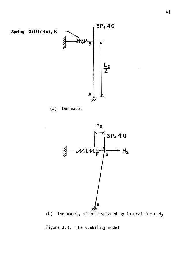
3.6 THE INELASTIC BUCKLING LOAD BY BOLTON'S METHOD

In a paper presented recently by A. Bolton (15) he has shown that

the elastic critical buckling load of a structure can be investigated

and calculated by using a simple model. The important matter is that

whatever is true for this model of the structure is also true for the

whole structure.

This model consists of a vertical rigid bar which is freely

pivotted at its base A, carries an axial load of (3P + 4Q) (the total

load in that story, which should be carried by the frame) at its upper

end B, and is supported by a linear spring of stiffness k connected at

B, Fig. 3.8a. The vertical bar AB is then displaced by a lateral force

of H2, causing a deflection of ~2 which in effect causes overturning

moment (P-~ effects) and elastic restoring forces from the linear spring.

1 ~

~ 41

Spring Stiffness, K ~3P+4Q

B

Le 2

(a) The model

A2

n3P .. 4Q

B • H2

(b) The model, after displaced by lateral force H2

Figure 3.8. The stability model

l i

42

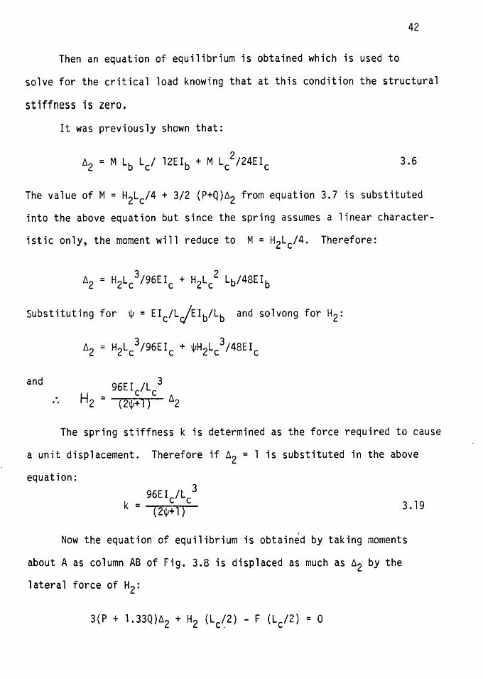
Then an equation of equilibrium is obtained which is used to

solve for the critical load knowing that at this condition the structural

stiffness is zero.

It was previously shown that:

A2 = M Lb Lc/ 12Elb + M Lc2/24Elc 3.6

The value of M = H2Lc/4 + 3/2 (P+Q)A2 from equation 3.7 is substituted

into the above equation but since the spring assumes a linear character-

istic only, the moment will reduce to M = H2Lc/4. Therefore:

3 2 A2 = H2Lc /96Elc + H2Lc Lb/48Elb

Substituting for ~ = EiclL/Eib/Lb and solvong for H2:

and .

A2 = H2Lc3/96Elc + wH 2Lc3/48Eic

3 96Elc/Lc

H 2 = ( 2'1.1+ 1) A2

The spring stiffness k is determined as the force required to cause

a unit displacement. Therefore if A2 = 1 is substituted in the above

equation:

k = --r=-- - 3. 19

Now the equation of equilibrium is obtained by taking moments

about A as column AB of Fig. 3.8 is displaced as much as A2 by the

lateral force of H2:

3(P + 1.33Q)A2 + H2 (Lc~2) - F (Lc/2) = 0

43

where F = the elastic restoring force in the spring = k * /j2

substituting for F = k * /j2 and simplifying

H2Lc/62 = klc - 6 (P + l.33Q)

But when axial load reaches its critical value, the structural stiffness

H 2 1~2 is zero, therefore

0 = klc - 6 (P + l.33Q)

or (P + l.33Q) = klc/6

substituting fork from equation 3.19

P + l.33Q = 16=Ic/L/

This equation is now divided by the critical buckling load, PE =

n2Eic/Lc2 to result the inelastic buckling load

i6 p + l.33Q = ~ 1) p TI ( 2o/+ E

3.20

which is the same as the previous solution.

3.7 ELASTIC INSTABILITY OF THE FRAME

Now let us examine the condition under which the frame will buckle

elastically, prior to formation of any hinges.

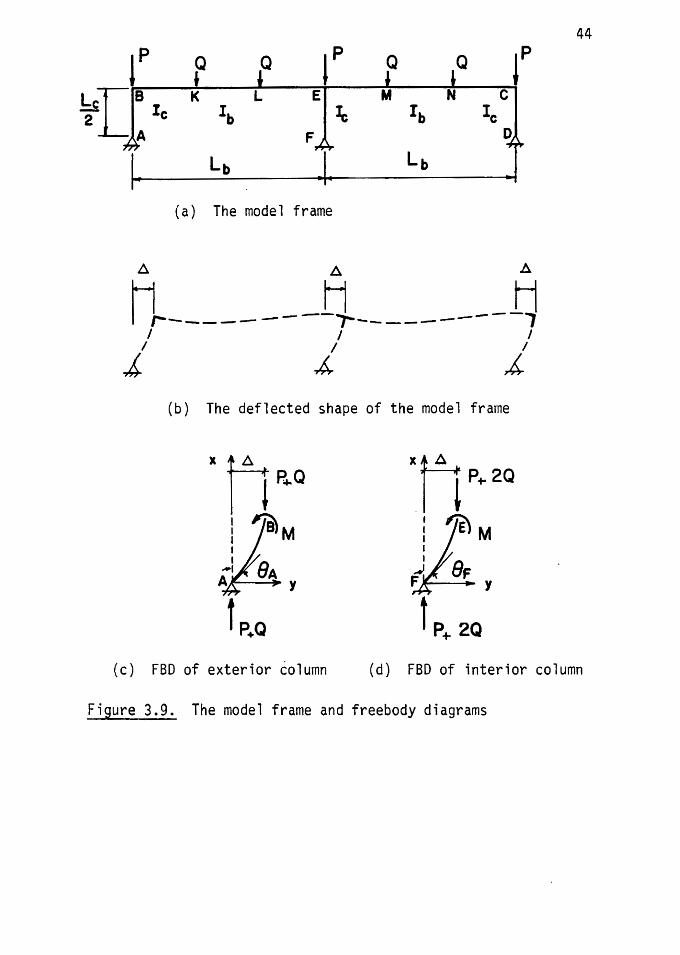
The model frame with its respective deflected shape and the free

body diagrams of exterior and interior columns are shown in Fig. 3.9.

Of course, knowing ~bottom and ~top' by means of Jackson and Moreland

nomograph one can find the effective column length factor A. But for

1

! I I . .

44

( Q !Q ( Q Q ( I I l ~c[~ le

K L

Fl~ M N c

Ib Ib IC D

Lb I Lb

(a) The model frame

~ ~ A

H _H __ ti I J.-. _____ -- ..,_______________ 1 I I I

I I I

_£_ A- £ (b) The deflected shape of the model frame

XH I i p+- 2a

y ~'ie)M

F F y

f P.Q t p+- 2Q

(c) FBD of exterior column (d) FBD of interior column

Figure 3.9. The model frame and freebody diagrams

I ! 1

45

more accuracy an exact solution is presented in the following.

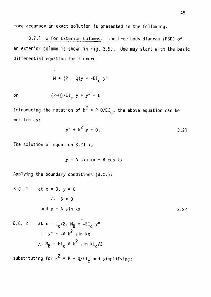
3.7.l A for Exterior Columns. The free body diagram (FBD) of

an exterior column is shown in Fig. 3.9c. One may start with the basic

differential equation for flexure

or

M = (P + Q)y = -Eic Y11

(P+Q)/EI y + y" = 0 c

Introducing the notation of k2 = P+Q/Elc, the above equation can be

written as:

y" + k2 y = 0.

The solution of equation 3.21 is

y = A sin kx + B cos kx

Applying the boundary conditions (B.C.):

B.C. 1

B. C. 2

at x = 0, y = 0

S = 0

and y = A sin kx

/

at x = Lc/2, Ms = -EIC y"

if y" = -A k2 sin kx

:. Ms = EIC A k2 sin kLC/2

substituting for k2 = P + Q/Eic and simplifying:

3.21

3.22

46

A = Ms/(P+Q) Sin KLC/2 3.23

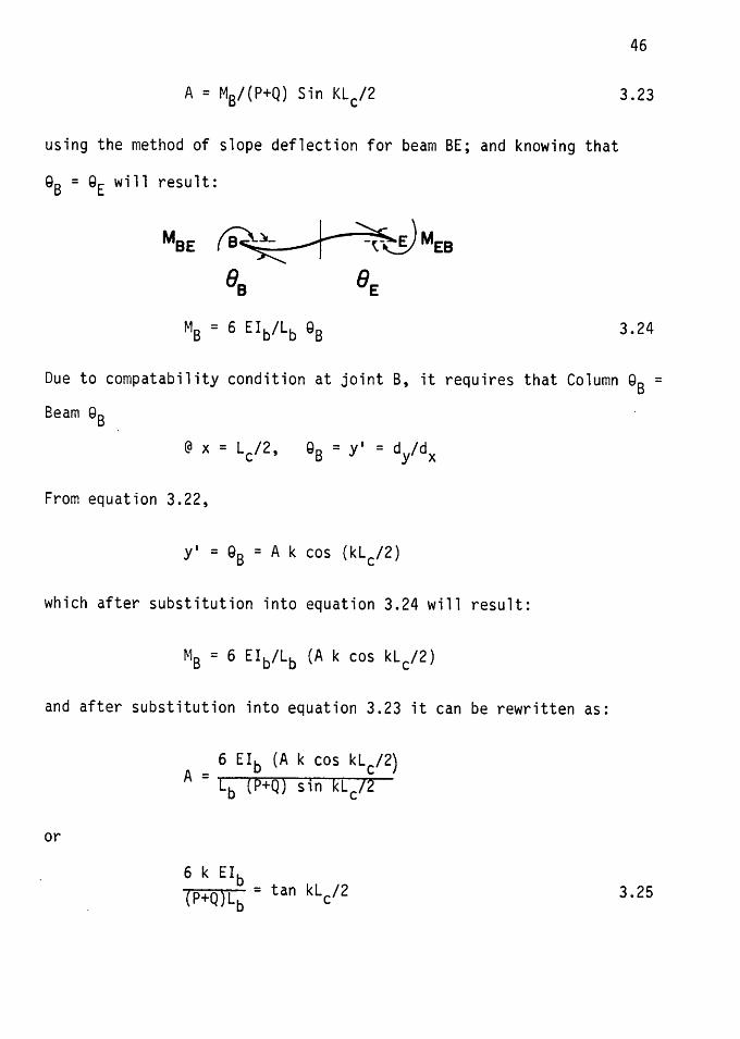
using the method of slope deflection for beam BE; and knowing that

QB = QE will result:

MBE ~~MEB 88 BE

MB = 6 Elb/Lb QB 3.24

Due to compatability condition at joint B, it requires that Column QB = Beam 98

@ x = L /2 Q = y' = d /d c ' B y x

From equation 3.22,

y' = QB = A k cos (kLc/2)

which after substitution into equation 3.24 will result:

M8 = 6 Elb/Lb (A k cos klc/2)

and after substitution into equation 3.23 it can be rewritten as:

or

6 Eib (A k cos klc/2) A = ..-[ b----.-(-p+-=Q-) -s ...... i n--....-k L-c-7-2 -

6 k Elb (P+Q)L = tan kl /2 b c

3.25

l i

47

now substituting for (P+Q)

3.25 it may be shown that:

into equation

(kLc/2)tan (klc/2)= 3/w 3.26

which is the stability equation for the exterior columns.

For example, if~= 2; substituting into equation 3.26:

(klc/2)tan (klc/2) = 3/2 = 1.5

Now by trial and error solution, one may find (klc/2) such that

the above equation is equal to 1.5.

or

klc/2 = 0.988 (radians)

k2 - 0.9761 - (Lc/2)2

substituting for k2 = Pcr/Elc, (where Per is the exterior column critical

load):

Per 0.9761 Eic = (L /2)2

c

or (0.976l)EIC p = --~,..._ er (L 12 )2

c

Equating the critical buckling load,

(0.976l)EIC n2 EIC

( L c /2) 2 = -( A-e~) 2=--(-L c-/-2 )-x-2

n2Eic with above: P - 2' er - ·). L /2) { e c

l I

48

will result, Ae to be equal to 3.18.

A summary of Ae for variety of~ values are shown in table 3.1.

3.7.2 A for Interior Column. The free body diagram of the interior

column is shown in Fig. 3.9d. Following the same procedure,as described

in the previous section, it may be shown that,

MEF A = (P+2Q) sin klc/2

3.27

By condition of equilibrium at joint E,

MEF + MEB + MEC = O

and due to symmetry of the frame,

QB = QEB = QEC = QC

by using the slope deflection method:

MEF = 12 Elb/Lb QE 3.28

Due to compatability condition at joint E, it requires that:

@ x = Lc/2, QE = y' = dy/dx

or y' = QE = A k cos klc/2

which after substituting into equation 3.28 and back substituting into

equation 3.27 it can be rewritten as:

12 Eib A k cos klc/2 A - --------=""T---....-..._. - Lb (P + 2Q) sin kLc/2

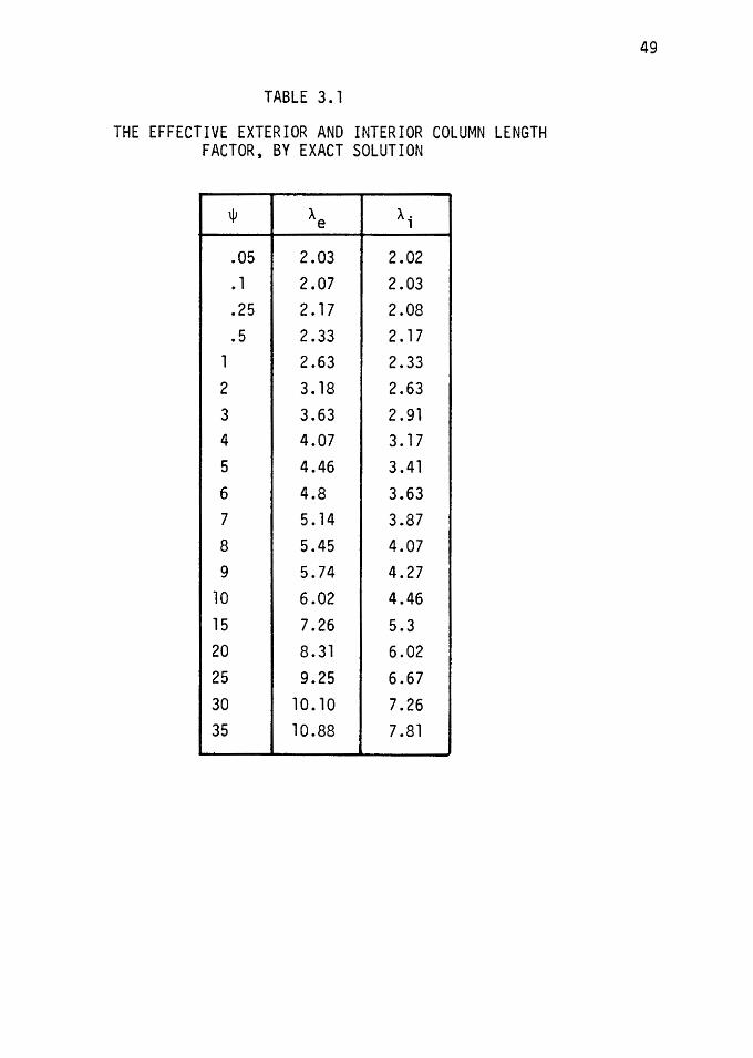
TABLE 3. 1

THE EFFECTIVE EXTERIOR AND INTERIOR COLUMN LENGTH FACTOR, BY EXACT SOLUTION

\jJ "'e A· 1

.05 2.03 2.02

. 1 2.07 2.03

.25 2. 17 2.08

.5 2.33 2. 17 1 2.63 2.33 2 3. 18 2.63 3 3.63 2.91 4 4.07 3. 17 5 4.46 3.41 6 4.8 3.63 7 5. 14 3.87 8 5.45 4.07 9 5.74 4.27

10 6.02 4.46 15 7.26 5.3 20 8.31 6.02 25 9.25 6.67 30 10.10 7.26 35 10.88 7.81

49

or klc

=tan~

50

3.29

2 Elc/Lc now, substituting for (P + 2Q) = k Eic and the value of ¢ = tI /L ,

b b

into equation 3.29, it may be shown that :

kl klc _ 6 (-f-) tan (~) - \j)

3.30

which is the stability equation for the interior column.

Again, for example if¢= 2, it will be determined that Ai = 2.63.

A summary of A; for variety of¢ values are shown in Table 3.1.

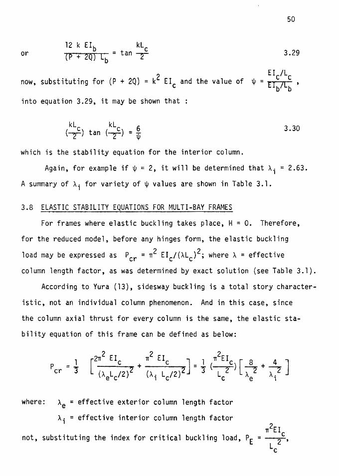
3.8 ELASTIC STABILITY EQUATIONS FOR MULTI-BAY FRAMES

For frames where elastic buckling takes place, H = O. Therefore,

for the reduced model, before any hinges form, the elastic buckling

load may be expressed as Per= n2 Elc/(ALc) 2; where A =effective

column length factor, as was determined by exact solution (see Table 3.1).

According to Yura (13), sidesway buckling is a total story character­

istic, not an individual column phenomenon. And in this case, since

the column axial thrust for every column is the same, the elastic sta­

bility equation of this frame can be defined as below:

2 2 2 l [2n E I c n EI c J l n E I c . [ B 4 J p = + =-;:-( ) -+

er ! (A L /2)"'! (A· L /2) 2 J L 2 A 2 ~ ec 1 c c e 1

where: Ae = effective exterior column length factor

Ai = effective interior column length factor n2EI

not, substituting the index for critical buckling load, PE = ----i-' LC

1

51

Per 2 -=";It" PE j

(4)+.!.{4) ~ j ~

e i

3.31

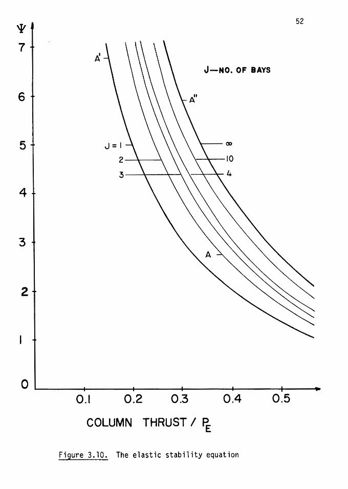
The graphical solution of the above equation, as a function of w, is

shown by curve A in Fig. 3.10, which represents the elastic stability

equation of a two-bay frame.

The elastic stability equation of frames with 3, 4, 10, or in

general J number of bays may be found and is summarized in Table 3.2.

These equations are all shown graphically in Fig. 3.10. It is important

to recognize that curve A' (for an exterior column or single-bay frame)

and curve A11 (for an interior column or many-bay frame) represent the

lower and upper bounds of the elastic stability equation. As the number

of bays increase, the elastic stability equation gets closer and closer

to the upp·er bound, as the effect of two exterior columns diminish.

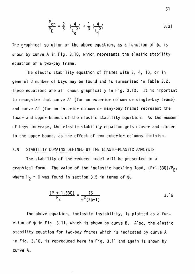
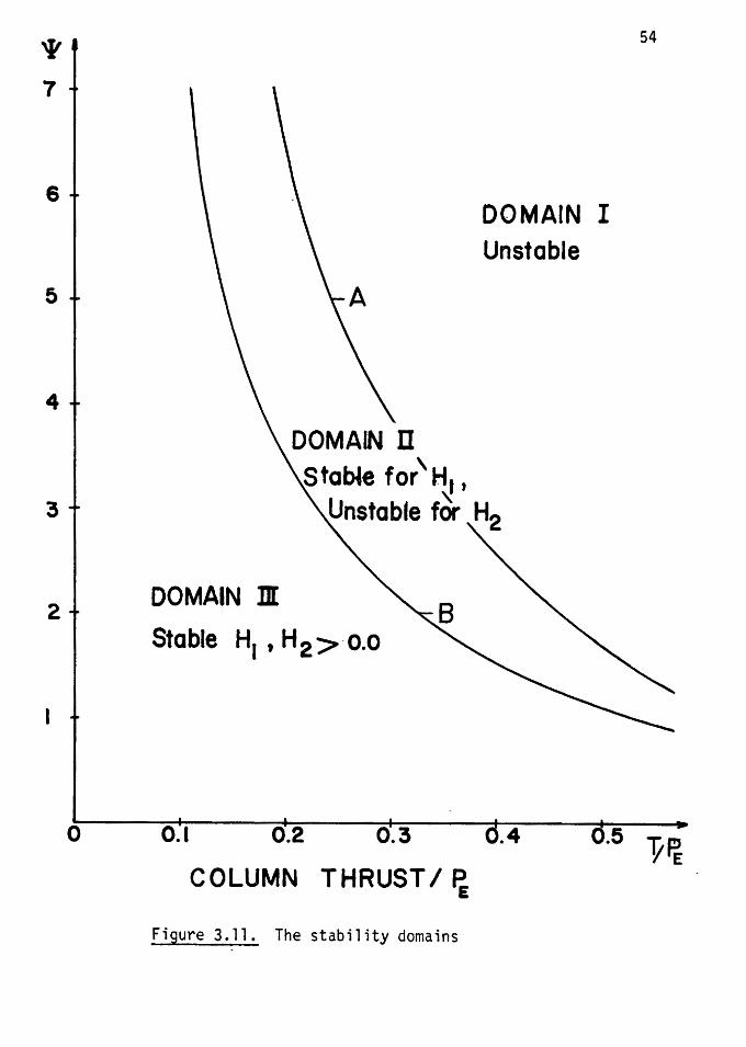
3.9 STABILITY DOMAINS DEFINED BY THE ELASTO-PLASTIC ANALYSIS

The stability of the reduced model will be presented in a

graphical form. The value of the inelastic buckling load, (P+l.33Q)/PE,

where H2 = 0 was found in section 3.5 in terms of ~,

3. 18

The above equation, inelastic instability, is plotted as a fun­

ction of win Fig. 3.11, which is shown by curve B. Also, the elastic

stability equation for two-bay frames which is indicated by curve A

in Fig. 3. 10, is reproduced here in Fig. 3.11 and again is shown by

curve A.

'I' 7

6

5

4

3

2

52

/!.. J-NO. OF BAYS

---00

~ \ \\\ll~

0 ...__ _ __...,_ __ .,____--+---+------+-----

0.1 0.2 0.3 0.4 0.5

COLUMN THRUST I Ff:

Figure 3.10. The elastic stability equation

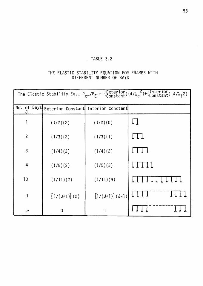
TABLE 3.2

THE ELASTIC STABILITY EQUATION FOR FRAMES WITH DIFFERENT NUMBER OF BAYS

53

. . . p /P _ (Exterior)( 4/ ~) (Interior)( 4/ 2) The Elastic Stab1l1ty Eq., er E - Constant Ae +Constant Ai

No. of Bays J

Exterior Constant Interior Constant

1 ( 1 /2) ( 2) ( 1/2)(0) f1

2 (l/3)(2) (1/3)(1) m 3 (1/4)(2) (1/4)(2) 1 11 l

4 (1/5)(2) (1/5)(3) 11111

10 (1/11) (2) (1/11)(9) 11111111111

J [ 1 I ( J+ 1 )] ( 2 ) [ 1 I ( J+ 1 ) J ( J- l ) I 111-·- ---·- l I 11

00 0 l 1 I I i-·-------rn

'I' 7

6

5

4

3

2

0

DOMAIN m

DOMAIN ll

DOMAIN I Unstable

\ Sta~ for H1,

'= Unstable for H2

Stable H1 , H2 >·o.o

54

OJ 0-.2 o-.3 .4 .5 v~ COLUMN THRUST I~

Figure 3.11. The stability domains

1

Curves A and B divide the total spectrum into three separate

domains. Domain I is to the right of curve A which represents the

frames that are unstable before any lateral load can be applied.

55

Therefore H1 and H2 = O. Domain II, which is the region which lies

between curves A and B, represent the frames that are stable only for

lateral loads up to H1. Therefore H2 = 0.

Domain III, which is to the left of curve B, represents the

frames that are stable until a mechanism forms. Therefore H1 and H2 > 0.

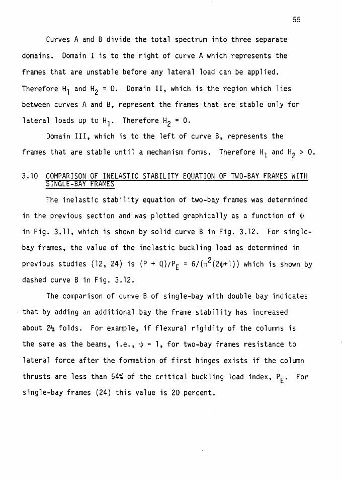
3. 10 COMPARISON OF INELASTIC STABILITY EQUATION OF TWO-BAY FRAMES WITH SINGLE-BAY FRAMES

The inelastic stability equation of two-bay frames was determined

in the previous section and was plotted graphically as a function of w

in Fig. 3. 11, which is shown by solid curve Bin Fig. 3.12. For single­

bay frames, the value of the inelastic buckling load as determined in

previous studies (12, 24) is (P + Q)/PE = 6/(n2(2w+l)) which is shown by

dashed curve Bin Fig. 3.12.

The comparison of curve B of single-bay with double bay indicates

that by adding an additional bay the frame stability has increased

about 2~ folds. For example, if flexural rigidity of the columns is

the same as the beams, i.e., w = 1, for two-bay frames resistance to

lateral force after the formation of first hinges exists if the column

thrusts are less than 54% of the critical buckling load index, PE. For

single-bay frames (24) this value is 20 percent.

'It 7

6

5

4

3

2

0

I I I I

' ' ' \ \ \ \

KEY - - - One Bay Frame - Two Bay Frame

DOMAIN I Unstable

56

\ \ \ \ DOMAIN II \ rB

\ \

' '

\ Sta~e for H1 , "\'.

Unstabie for H2

DOMAIN m Stable

OJ

HI , H2> o.o

' ' ' ' ', ', --..........._,

0-.2 o-.3 ..._--. .__ -- -- - - --

.4

COLUMN THRUST I~

Figure 3.12. Stability domains for one and two bay frames

CHAPTER IV

COMPUTER ANALYSIS

4.1 GENERAL

In this chapter, the stability of unbraced frames will be investi­

gated using a computer program. This program is applied to twenty rec­

tangular model frames with the same overall geometry. Fourteen frames

have the same low column reinforcement ratio of 2% but different loading

conditions and cross sections. The remaining six frames have the

same high reinforcement ratio of 8% but different loading conditions

and cross sections.

The column reinforcement ratio (Pg) of 2% was chosen to represent

a practical value representative of columns in buildings. The maximum

value of 8% was chosen to represent the upper limit of column reinforce-

ment according to ACI 318-77, Art. 10.9.l (4). All beams were assumed

to possess a reinforcement ratio p = 1%.

4.2 DESCRIPTION OF THE COMPUTER PROGRAM

The computer program used in this investigation is program

NONFIX7 (12), which is a version of the computer program NONFIX5, ori­

ginally developed by Gunnin (16) and later modified by Rad (12). The

program is a generalized computational method for nonlinear analysis of

planar frames, and takes nonlinear geometry and nonlinear force defor­

mation properties (thrust-moment-curvature, P-M-0) of the members into

account. The P-M-0 relationships for individual members are constructed

using a computer program originally dev~loped by Breen (17) which assumes

the Hognestad's (18) stress-strain curve relationship for concrete in

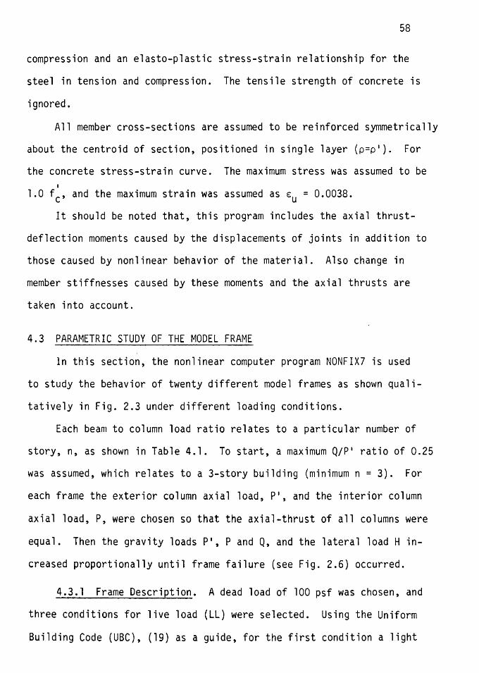
58

compression and an elasto-plastic stress-strain relationship for the

steel in tension and compression. The tensile strength of concrete is

ignored.

All member cross-sections are assumed to be reinforced symmetrically

about the centroid of section, positioned in single layer (p=p'). For

the concrete stress-strain curve. The maximum stress was assumed to be I

1.0 fc, and the maximum strain was assumed as €u = 0.0038.

It should be noted that, this program includes the axial thrust-

deflection moments caused by the displacements of joints in addition to

those caused by nonlinear behavior of the material. Also change in

member stiffnesses caused by these moments and the axial thrusts are

taken into account.

4.3 PARAMETRIC STUDY OF THE MODEL FRAME

In this section, the nonlinear computer program NONFIX7 is used

to study the behavior of twenty different model frames as shown quali­

tatively in Fig. 2.3 under different loading conditions.

Each beam to column load ratio relates to a particular number of

story, n, as shown in Table 4.1. To start, a maximum Q/P' ratio of 0.25

was assumed, which relates to a 3-story building (minimum n = 3). For

each frame the exterior column axial load, P', and the interior column

axial load, P, were chosen so that the axial-thrust of all columns were

equal. Then the gravity loads P', P and Q, and the lateral load Hin­

creased proportionally until frame failure (see Fig. 2.6) occurred.

4.3.l Frame Description. A dead load of 100 psf was chosen, and

three conditions for live load (LL) were selected. Using the Uniform

Building Code (UBC), (19) as a guide, for the first condition a light

59

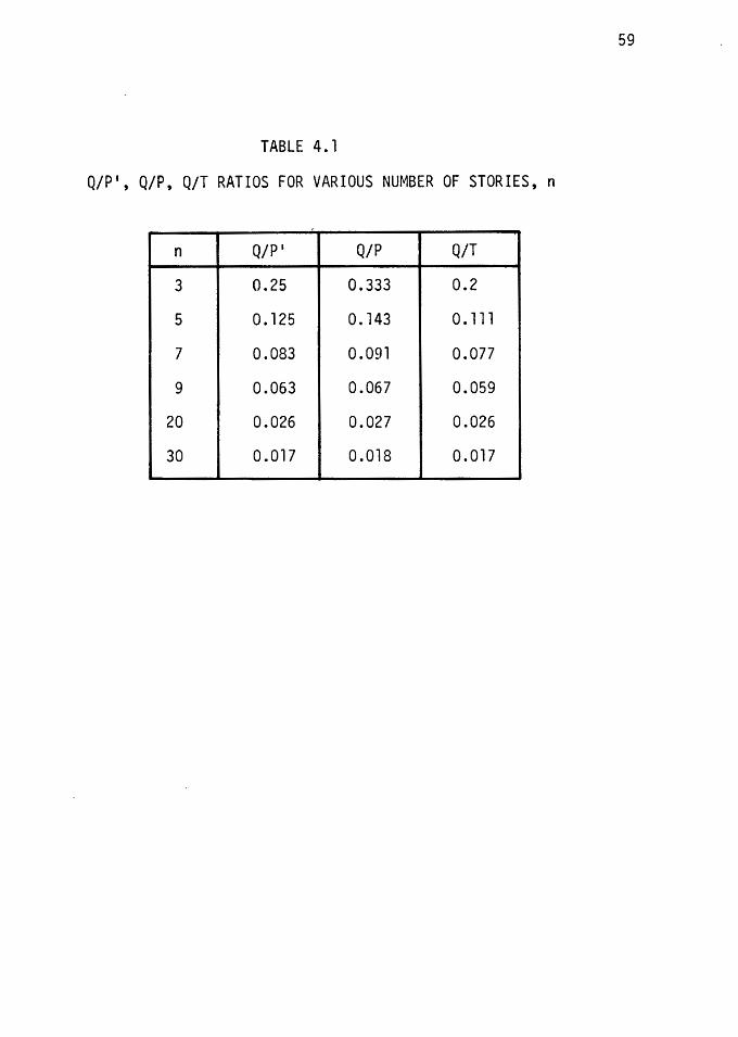
TABLE 4. 1

Q/P', Q/P, Q/T RATIOS FOR VARIOUS NUMBER OF STORIES, n

n Q/P' Q/P Q/T

3 0.25 0.333 0.2

5 0.125 0. 143 0. 111

7 0.083 0.091 0.077

9 0.063 0.067 0.059

20 0.026 0.027 0.026

30 0.017 0.018 0.017 I

60

live load of 50 psf, for the second condition a medium live load of

150 psf, and for the third condition a heavy live load of 250 psf were

selected.

The height of the columns (Lc) and the length of the beams (Lb)

were 42-in and 84 in respectively. Column and beam sections were rein­

forced symmetrically with respect to the centroid of the section on

two opposite faces in a single layer, throughout the length of the

member (p=p'). The thickness of concrete cover, measured from face

to center of the nearest steel bar, de, was assumed as 0.75 in. A

width b = 6 in was assumed for both beam and column sections. For

the cases of 20 and 30 stories for the beam section, a width b = 7"

and for the column sections a width b = 811 and b = 10" were assumed

respectively.

The center to center spacing of the frames was assumed to be equal

to 84-in, i.e., same as Lb. Grade 60 steel reinforcement (fy = 60 ksi)

and the concrete strength f~ = 4000 psi were used. All frames were

chosen to approximate a one-third scale factor (SF= 1/3).

Design of beams and columns of a typical frame is discussed in

the following sections. The only variables were Q/P' ratio, loading

condition, and column reinforcement ratio.

4.3.2 Design of Beams. All beam sections were designed to carry

the gravity load. After the desired loading condition was selected,

using equations 9-1 of the ACI-Code (4), the ultimate loads were deter-

mined~ Then by moment distribution method, moments were calculated and

beams were designed. An example of the above design procedure for con-

dition of light live load, i.e., LL= 50 psf; is shown below. Note that,

an equal reinforcement ratio of one percent, p = 1%, for bottom and top

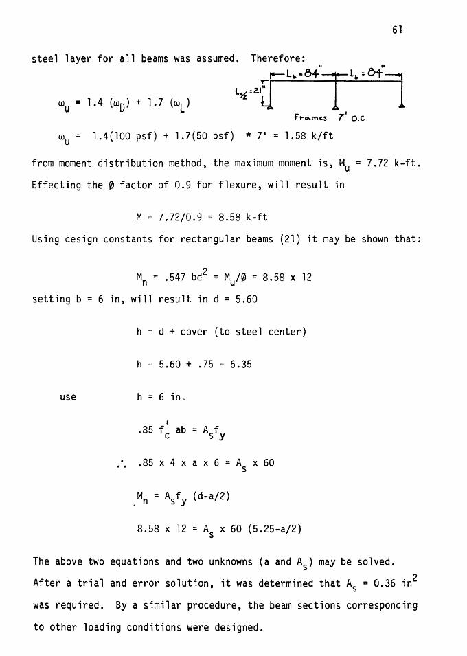
61

steel layer for all beams was assumed. Therefore: II "

wu = 1.4 (w0) + 1.7 (wl)

.,._1-L •• e+ i L• = o+ ----, L~·~·~ 1

Ft"o..IT'l~S 7' o.c..

wu = 1.4(100 psf) + 1.7(50 psf) * 71 = 1.58 k/ft

from moment distribution method, the maximum moment is, Mu = 7.72 k-ft.

Effecting the 0 factor of 0.9 for flexure, will result in

M = 7.72/0.9 = 8.58 k-ft

Using design constants for rectangular beams (21) it may be shown that:

2 Mn = .547 bd = Mu/0 = 8.58 x 12

setting b = 6 in, will result in d = 5.60

h = d + cover (to steel center)

h = 5.60 + .75 = 6.35

use h = 6 in.

I

.85 f cab= Asf y

:. .85 x 4 x a x 6 = As x 60

.Mn= Asfy {d-a/2)

8.58 x 12 = As x 60 (5.25-a/2)

The above two equations and two unknowns (a and As) may be solved.

After a trial and error solution, it was determined that As = 0.36 in2

was required. By a similar procedure, the beam sections corresponding

to other loading conditions were designed.

62

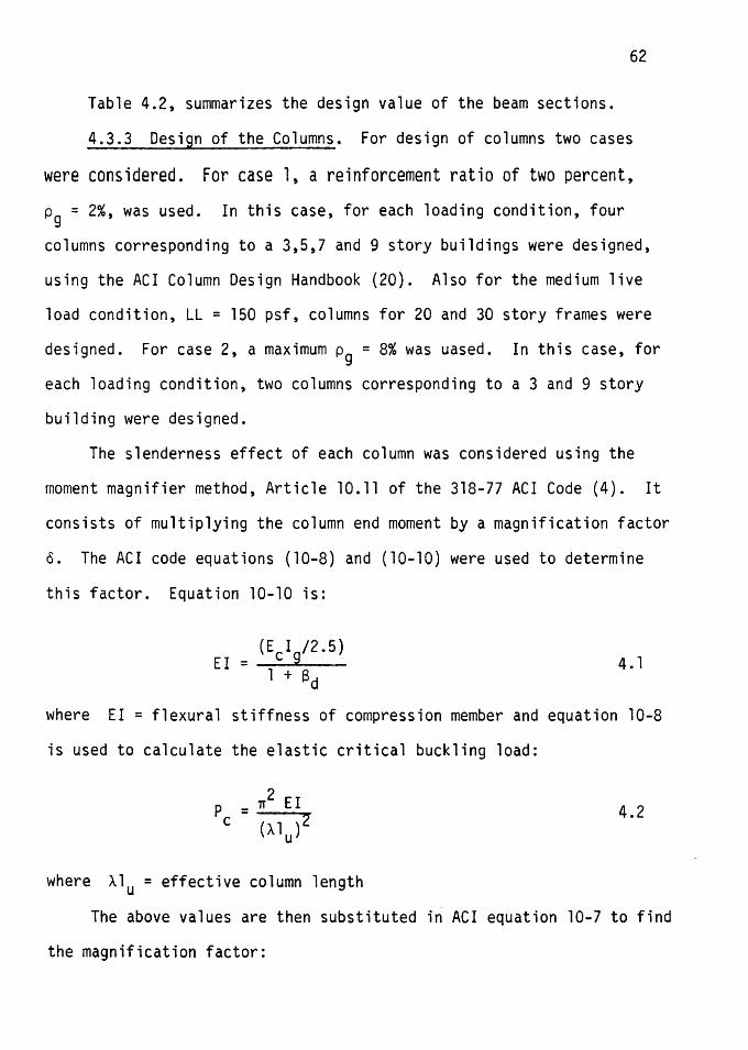
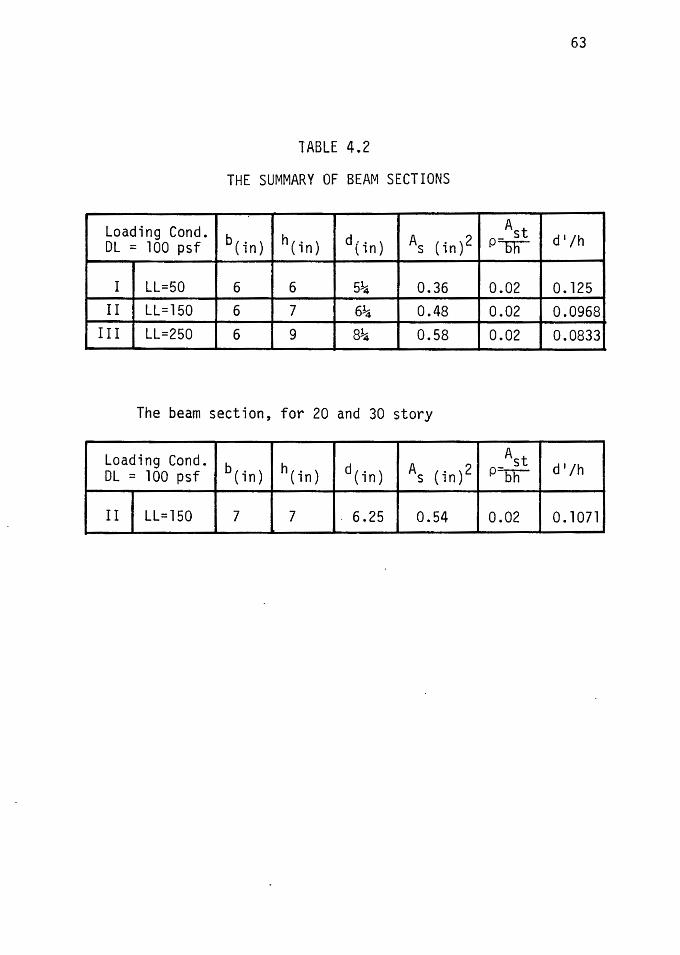
Table 4.2, summarizes the design value of the beam sections.

4.3.3 Design of the Columns. For design of columns two cases

were considered. For case 1, a reinforcement ratio of two percent,

Pg = 2%, was used. In this case, for each loading condition, four

columns corresponding to a 3,5,7 and 9 story buildings were designed,

using the ACI Column Design Handbook (20). Also for the medium live

load condition, LL = 150 psf, columns for 20 and 30 story frames were

designed. For case 2, a maximum Pg = 8% was uased. In this case, for

each loading condition, two columns corresponding to a 3 and 9 story

building were designed.

The slenderness effect of each column was considered using the

moment magnifier method, Article 10.11 of the 318-77 ACI Code (4). It

consists of multiplying the column end moment by a magnification factor

c. The ACI code equations (10-8) and (10-10) were used to determine

this factor. Equation 10-10 is:

(E I /2 EI = c g .5~ 1 + B d

4. 1

where EI = flexural stiffness of compression member and equation 10-8

is used to calculate the elastic critical buckling load:

p c

where Alu = effective column length

4.2

The above values are then substituted in ACI equation 10-7 to find

the magnification factor:

63

TABLE 4.2

THE SUMMARY OF BEAM SECTIONS

Loading Cond. A t DL = 100 psf b (in) h (in) d (in) As (in) 2 p=oF- d'/h

I LL=50 6 6 5~ 0.36 0.02 0. 125 II LL=l50 6 7 6~ 0.48 0.02 0.0968

III LL=250 6 9 8~ 0.58 0.02 0.0833

The beam section, for 20 and 30 story

Loading Cond. b (in) h(in) d(in) A s (in) 2

Ast d'/h DL = 100 psf p-bh

II LL=l50 7 7 . 6.25 0.54 0.02 0. 1071

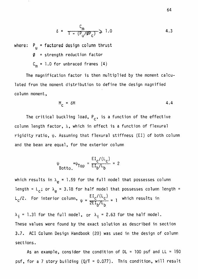
cm o = l _ ( p 70P ) ~ 1. o

u c

where: Pu = factored design column thrust

0 = strength reduction factor

cm= 1.0 for unbraced frames (4)

64

4.3

The magnification factor is then multiplied by the moment calcu­

lated from the moment distribution to define the design magnified

column moment,

M = 6M c 4.4

The critical buckling load, Pc, is a function of the effective

column length factor, A, which in effect is a function of flexural

rigidity ratio, ~. Assuming that flexural stiffness (EI) of both column

and the beam are equal, for the exterior column

w =w = EIC/(Lc) Botto. Top Elb/Lb = 2

which results in Ae = 1.59 for the full model that possesses column

length= Lc; or Ae = 3.18 for half model that possesses column length=

Lc/2. For interior column, ~ _ Eic/(Lc) _ 1 which results in - 2Eib/Lb -

Ai = 1.31 for the full model, or Ai = 2.63 for the half model.

These values were found by the exact solution as described in section

3.7. ACI Column Design Handbook (20) was used in the design of column

sections.

As an example, consider the condition of DL = 100 psf and LL = 150

psf, for a 7 story building (Q/T = 0.077). This condition, will result

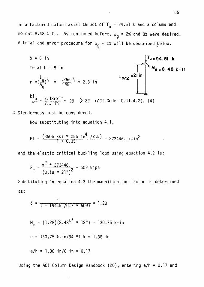
65

in a factored column axial thrust of Tu = 94.51 k and a column end ·

moment 8.48 k-ft. As mentioned before, Pg = 2% and 8% were desired.

A trial and error procedure for Pg = 2% will be described below.

b = 6 in

Trial h = 8 in

r =(:g)~ = (~)~ = 2.3 in g

1Tu:94.51 k

~Mu =8.48 k-ft

L :21 in C/2

klu = 3.18*:21"= 29 ) 22 (ACI Code 10.11.4.2), (4) r '5 ') ., ...

~ Slenderness must be considered.

Now substituting into equation 4.1,

(3605 ksi * 256 in4

/2.5) = 273446. k-in2 EI = · ~ ~~

and the elastic critical buckling load using equation 4.2 is:

TI2 * 273446. = 609 kips Pc=. 18 * 21")2 (3.

Substituting in equation 4.3 the magnification factor is determined

as:

l 0: 1 JnA r-11"., _._ ,-"X\: 1.28

Mc = ( 1. 28 )( 8. 48k 1 * 12 11

) = 130: 75 k-i n

e = 130.75 k-in/94.51 k = 1.38 in

e/h = 1.38 in/8 in= 0.17

Using the ACI Column Design Handbook (20), entering e/h = 0.17 and

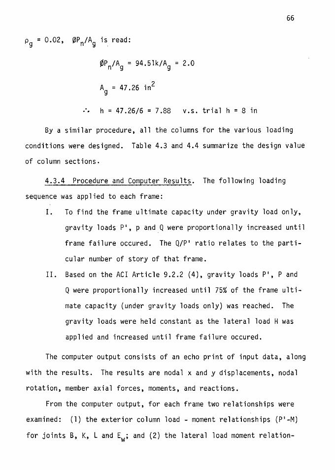
66

Pg = 0.02, 0Pn/A9 is read:

¢Pn/A9

= 94.51k/A9 = 2.0

A9

= 47.26 in2

.. h = 47.26/6 = 7.88 v.s. trial h = 8 in

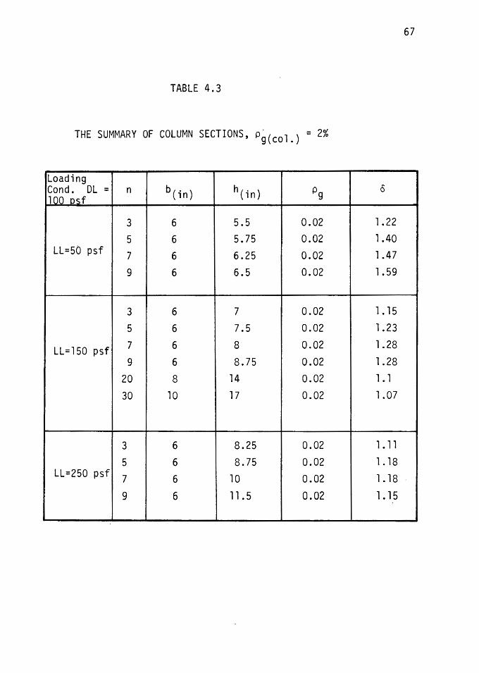
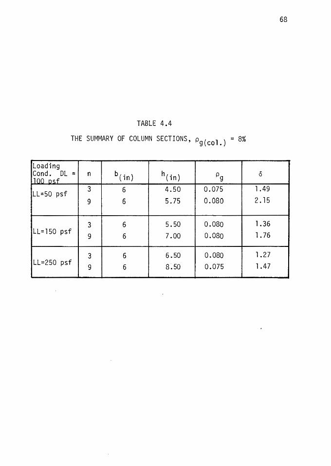
By a similar procedure, all the columns for the various loading

conditions were designed. Table 4.3 and 4.4 summarize the design value

of column sections.

4.3.4 Procedure and Computer Results. The following loading

sequence was applied to each frame:

I. To find the frame ultimate capacity under gravity load only,

gravity loads P', p and.Q were proportionally increased until

frame failure occured. The Q/P' ratio relates to the parti­

cular number of story of that frame.

II. Based on the AC! Article 9.2.2 (4), gravity loads P', P and

Q were proportionally increased until 75% of the frame ulti­

mate capacity (under gravity loads only) was reached. The

gravity loads were held constant as the lateral load H was

applied and increased until frame failure occured.

The computer output consists of an echo print of input data, along

with the results. The results are nodal x and y displacements, nodal

rotation, member axial forces, moments, and reactions.

From the computer output, for each frame two relationships were

examined: (1) the exterior column load - moment relationships (P'-M)

for joints B, K, L and Ew; and (2) the lateral load moment relation-

67

TABLE 4.3

THE SUMMARY OF COLUMN SECTIONS, Pg(col.) = 2%

Loading Cond. DL = n b (in) h (in) Pg 8 100 osf

3 6 5.5 0.02 1.22

5 6 5.75 0.02 1.40 LL=5b psf 7 6 6.25 0.02 1.47

9 6 6.5 0.02 1.59

3 6 7 0.02 1. 15

5 6 7.5 0.02 1.23

LL=l50 psf 7 6 8 0.02 1.28

9 6 8.75 0.02 1.28

20 8 14 0.02 1. 1

30 10 17 0.02 1.07

3 6 8.25 0.02 1.11

5 6 8.75 0.02 1. 18 LL=250 psf 7 6 10 0.02 1.18

9 6 11. 5 0.02 l. 15

68

TABLE 4.4

THE SUMMARY OF COLUMN SECTIONS, Pg(col.) = 8%

Loading b (in) h(in) Pg cS Cond. DL = n

100 nd

3 6 4.50 0.075 1.49 LL=50 psf

6 5.75 0.080 2. 15 9

3 6 5.50 0.080 1.36 LL=l50 psf

9 6 7.00 0.080 1. 76

3 6 6.50 0.080 1.27 LL=250 psf

9 6 8~50 0.075 1.47

l 69

ships (H-M) for joints B, K, L, E, M, N and C. From the P'-M relation­

ships, it was determined whether the plastic hinges form in the beam

or column at corners E and C.

The most useful plots are the H-M curves, which is used to study

the inelastic behavior of the frames. From these curves the level

of lateral load (H1) causing the first hinges at corners Ew and C,

and the level of lateral load (H2) causing the second hinges at K and M

to produce a combined mechanism were determined.

For some particular cases, the lateral load-deflection relationship

(H-~) were studied. The H-~ relationship does give some idea about

the level of lateral load (H2) but not as accurately as the H-M response

(14).

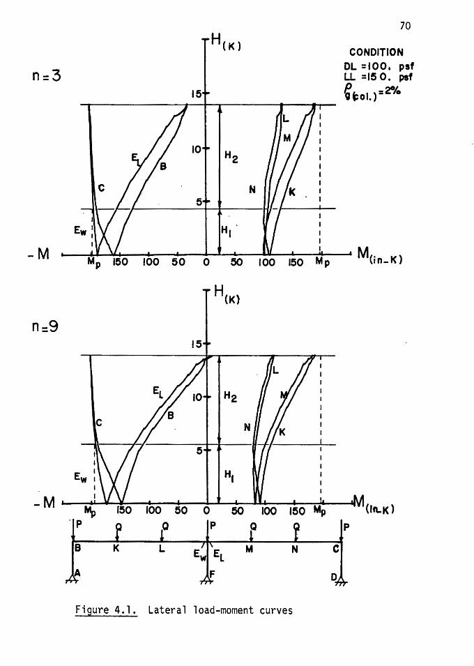
The response of each individual frame was studied by plotting a

set of (H-M) curves for corners B, C and E and joints K, L, M and H.

Each of these sets is identified by a different Q/P 1 ratio (n stories),

and were plotted by using a Tektronix 4051 plotter. As an example,

let us consider the behavior of the frames in medium loading condition

(DL = 100 psf, LL = 150 psf) and column Pg = 2% which are shown in

Fig. 4.1 and 4.2. It appears that the curves essentially consist of

two approximately linear parts which are connected together by a curved

segment. The bending moment capacity for a particular condition is

MP and is shown by a single value. At zero lateral load, the moments

are at 75% of frame capacity under gravity loads. With increasing

lateral load, the moments at B, C, E and K, L, M, N change almost

linearly until the bending moment capacity is reached at Ew and C.

The lateral load at this level is denoted by (H 1). As the lateral load

n:3

-M

n:9

H( K)

15

70

CONDITION DL =100. psf LL =15 0. psf

~ tol.) :2°/o

' u 'f5o 100 510 o ' 5o 1~~ 150 Mp ' M(in-K)

H(K)

15

- M ' ~ v r!o rbo ~o & ' 5o "100 1~0 M:i •rvi Clll-K l ·•p p

Figure 4.1. Lateral load-moment curves

n= 20 H (K)

15

Ew

CONDITION

DL = 100. pat LL =150. p1f

e< ,>=2% g co.

I I I I I

- M' ~P ifo 100 5o ), t 510

1 100 150 M~ ·M (in_ Kl

n:30 H (K)

15

10

I

Ew 1 N,L

71

-M • ~ }If • , I i , 1 , • :, • Mc . ~ 150 100 50 0 50 100 150 Mp '"- K)

p p p

B

A

Figure 4.2. Lateral Load-moment curves

72

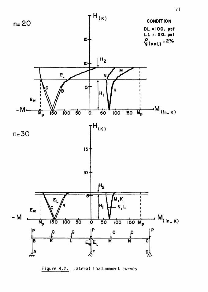
increases, the moments· at K and M increase more rapidly due to the

reduced frame stiffness caused by hinging at Ew and C, while the moments

at the later nodes remain unchanged at MP. Also the moments at B and

EL unwind rapidly to approximately zero. The moments at L and N slightly

increase. After the plastic moment capacity MP is reached at K and M,

these locations constitute the second set of plastic hinges. A combined

mecranism is then developed and frame is no longer stable failing in a

swa motion.

The studies made from behavior of n = 9 stories in Fig. 4.1 in­

dicate that in comparison with n = 3 stories, the lateral load capacity

of frame at the level which first hinges form (H 1) increases but the·

level at which second hinges form (H2) decreases.

The behavior of 20 and 30 stories are shown in Fig. 4.2. Their

response in comparison with 3 and 9 stories indicate that as the

number of stories increases, the lateral load capacity of frame at the

level which second hinges form (H 2) to produce a combined mechanism

decreases. For the case of 30 stories in Fig. 4.2, H2 is approximately

zero, which indicates the frame after the formation of first hinges

becomes unstable and fails.

These differences from 3 to 30 stories are due to the higher

column thrust-deflection (P-~) moments which are caused by the higher

column thrusts in the frame.

CHAPTER V

COMPARISON OF RESULTS BY TWO METHODS

5.1 GENERAL

In this section the frames analyzed in Chapter IV by computer pro­

gram NONFIX7 are compared with the stability domain of Fig. 3.11.

For all the frames, dead load was kept constant at 100 psf, but three

live load conditions (1) light LL = 50 psf, medium LL = 150 psf, and

heavy LL = 250 psf were selected. Columns in fourteen frames contai-

ned reinforcement ratio of 2%, and the remaining six frames had a

reinforcement ratio of 8% which is the maximum reinforcement ratio

permitted by the ACI Code.

5.2 COMPUTER RESULTS VS. STABILITY DOMAIN ANALYSIS

lhe computer results for each condition are shown in Tables 5.1

and 5.2. These tables give the column thrust T, lateral load capacity

H along with H1, H2, and the redistribution index S = H2/H.

Plots of moment redistribution index S as a function of the

number of stories, n, for 3 to 9 story frames with column Pg = 2%

and 8% are shown in Fig. 5.1. This figure shows the capacity of the

frame after the first hinge decreases as stories vary from 3 to 9.

The slope of each line appears to be approximately constant. As

loading becomes heavier, the p~rcent of moment redistribution appears

to increase slightly. Also for a specific n, S decreases as percent

reinforcement varies from 2% to 8%.

To determine the behavior of these frames beyond n = 9,

S vs. n is plotted for medium loading condition (DL = 100 psf, LL =

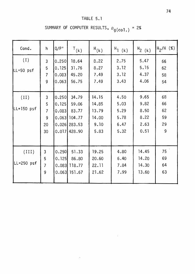
74

TABLE 5.1

SUMMARY OF COMPUTER RESULTS, Pg(col.) = 2%

Cond. h Q/P' T(k) H(k) Hl ( k) H2 ( k) H2/H (%)

( I) 3 0.250 18.64 8.22 2.75 5.47 66

LL=50 psf 5 0.125 31. 76 8.27 3. 12 5. 15 62

7 0.083 45.20 7.49 3. 12 4.37 58 9 0.063 56.75 7.49 3.43 4.06 54

(II) 3 0.250 34.79 14. 15 4.50 9.65 68

5 0. 125 59.06 14.85 5.03 9.82 66 LL=l50 psf 7 0.083 83. 77 13.79 5.29 8.50 62

9 0.063 104. 77 14.00 5.78 8.22 59

20 0.026 283.53 9. 10 6.47 2.63 29

30 0.017 428.90 5.83 5.32 0.51 9

(I II) 3 0.250 51.33 19.25 4.80 14.45 75

5 0. 125 86.80 20.60 6.40 14.20 69 LL=250 psf

7 0.083 118.77 22.11 7.84 14.30 64

9 0.063 151.67 21.62 7.99 13.60 63

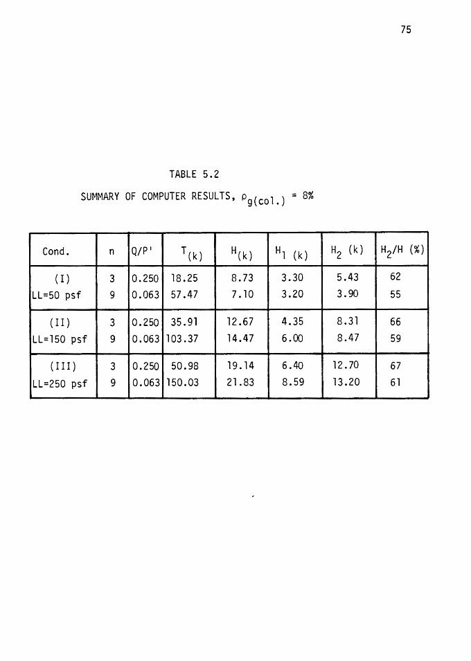
75

TABLE 5.2

SUMMARY OF COMPUTER RESULTS, Pg(col.) = 8%

Cond. n Q/P' T(k) H(k) Hl ( k) H2 ( k) H2/H (%)

(I) 3 0.250 18.25 8.73 3.30 5.43 62

LL=50 psf 9 0.063 57.47 7. 10 3.20 3.90 55

(II) 3 0.250 35.91 12.67 4.35 8.31 66

LL=l50 psf 9 0.063 103.37 14.47 6 .oo 8.47 59

(I II) 3 0.250 50.98 19. 14 6 .40 12.70 67

LL=250 psf 9 0.063 150.03 21.83 8.59 13.20 61

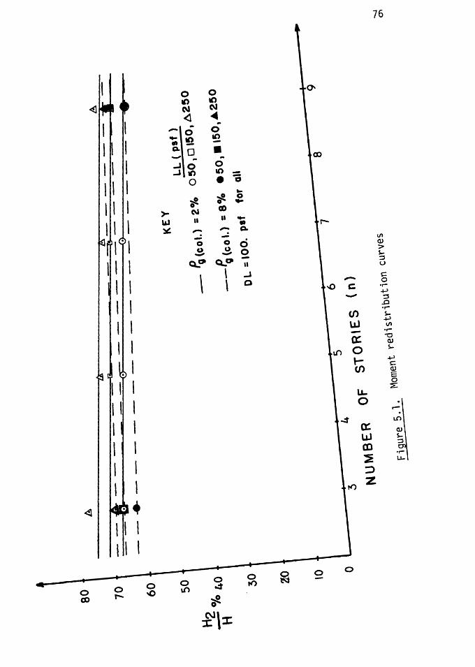
80

70

60

50

~O/o

40

H

30 ao

\0 0

A

.----~

.. -

----

·-·-

--

---

----------

KEY

L

L (

psf

)

-P

otco

l.)

:20

/o

05

0,0

l50

,A2

50

--~{

col.

) =

80/o

e5

0,

• 15

0,.A

.250

0 L

= \0

0.

psf

fo

r a\

\

3 4

NU

MB

ER

O

F

5 6

sT

OR

\ES

{

n)

7 8

9

f_]g

ure

s.1.

M

omen

t re

dist

ribu

tion

cur

ves

-.l

O

'

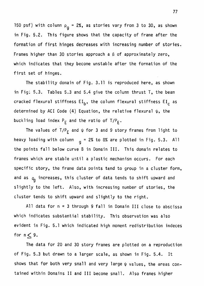
77

150 psf) with column Pg = 2%, as stories vary from 3 to 30, as shown

in Fig. 5.2. This figure shows that the capacity of frame after the

formation of first hinges decreases with increasing number of stories.

Frames higher than 30 stories approach a 6 of approximately zero,

which indicates that they become unstable after the formation of the

first set of hinges.

The stability domain of Fig. 3.11 is reproduced here, as shown

in Fig: 5.3. Tables 5.3 and 5.4 give the column thrust T, the beam

cracked flexural stiffness Elb, the column flexural stiffness Elc as

determined by ACI Code (4) Equation, the relative flexural ~' the

buckling load index PE and the ratio of T/PE.

The values of T/PE and ~for 3 and 9 story frames from light to

heavy loading with column g = 2% to 8% are plotted in Fig. 5.3. All

the points fall below curve B in Domain III. This domain relates to

frames which are stable u:1til a plastic mechanism occurs. For each

specific story, the frame data points tend to group in a cluster form,

and as Pg increases, this cluster of data tends to shift upward and

slightly to the left. Also, with increasing number of stories, the

cluster tends to shift upward and slightly to the right.

All data for n = 3 through 9 fall in Domain III close to abscissa

which indicates substantial stability. This observation was also

evident in Fig. 5.1 which indicated high moment redistribution indeces

for n< 9.

The data for 20 and 30 story frames are plotted on a reproduction

of Fig. 5.3 but drawn to a larger scale, as shown in Fig. 5.4. It

shows that for both very small and very large¢ values, the areas con­

tained within Domains II and III become small. Also frames higher

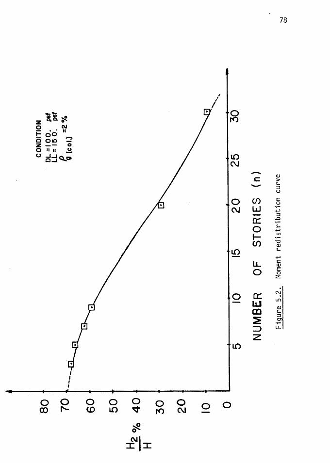
80

10

r----

60

50

H2

0; 0

4

0

H

30

20

10 0

----~·---

---·

---

-----· ---~·-----

CO

ND

ITIO

N

. D

L =

I 0 0

. ps

f L

L=

15

0.

psf

~(co

l.)

=2 %

5 I 0

15

2

0 2

5

30

NU

MB

ER

O

F S

TO

RIE

S

(n)

Fig

ure

5.2.

M

omen

t re

dis

trib

uti

on

cur

ve

,, .....

..

.......

co

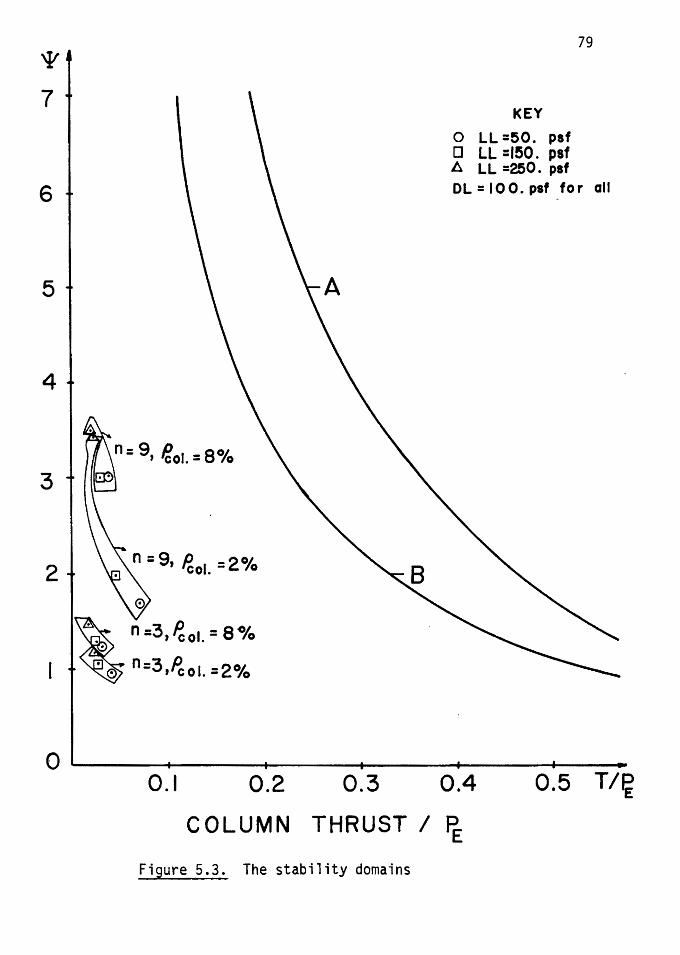
l

'1'

7

6

5

4

3

2 n = 9, Pco1. = 2°/o

0 \l

~ "=3,~01.=8% ·~ "=3,Pco1. =2%

KEY 0 LL =50. psf D LL =150. psf ~ LL =250. psf

79

DL = 100. psf for all

0-------+------+-----_._------+---~~-----0.1 0.2 0.3 0.4 0.5 Tl~

COLUMN THRUST I fE:

Figure 5.3. The stability domains

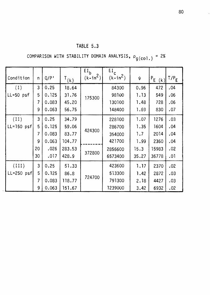
80

TABLE 5.3

COMPARISON WITH STABILITY DOMAIN ANALYSIS, Pg(col.) = 2%

Eib Eic Condition n Q/P' T(k) (k-in2) (k-in2) w PE (k) T/PE

(I) 3 0.25 18.64 84300 0.96 472 .04 LL=50 psf 5 o. 125 31. 76 175300 98100 1.13 549 .06

7 0.083 45.20 130100 1.48 728 .06 9 0.063 56.75 148400 1.69 830 .07

(II) 3 0.25 34.79 228100 1.07 1276 .03 LL=l50 psf 5 0. 125 59.06 286700 1.35 1604 .04

7 0.083 83. 77 424300

1. 7 2014 .04 354000 9 0.063 104.77 421700 1.99 2360 .04

~-------·

20 .026 283.53 2856600 15.3 15983 .02 30 .017 428.9

372800 6573400 35.27 36778 .01

(I I I) 3 0.25 51.33 423600 1. 17 2370 .02 LL=250 psf 5 0. 125 86.8 513300 1.42 2872 .03

7 0.083 118.77 724700

791300 2. 18 4427 .03 9 0.063 151.67 1239000 3.42 6932 .02

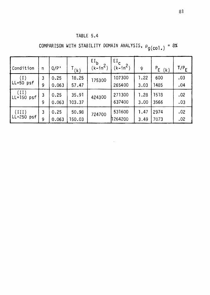
81

TABLE 5.4

COMPARISON WITH STABILITY DOMAIN ANALYSIS, Pg(col.) = 8%

Elb Elc Condition n Q/P' T(k) (k-in2) (k-in2) w PE (k) T/PE

( I ) 3 0.25 18.25 175300 107300 l.22 600 .03 LL=50 psf 9 0.063 57.47 265400 3.03 1485 .04

(I I) 3 0.25 35.91 271300 1.28 1518 .02 LL=l50 psf 424300 9 0.063 103.37 637400 3.00 3566 .03

(I I I) 3 0.25 50.98 724700 531600 1.47 2974 .02 LL=250 psf 9 0.063 150.03 1264200 3.49 7073 .02

'!'

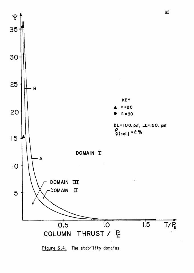
35

30

25

20

15

10

5

8

DOMAIN I

DOMAIN m n

0.5 1.0

KEY .._ n=20

• n =30

82

DL= 100. psf, LL=l!SO. paf

~(col.)= 2 %

1.5 T/~ COLUMN THRUST I fE

Figure 5.4. The stability domains

83

than 30 stories tend to fall close to Domain II, which indicates that

they become unstable after the first hinges form. This was also evi­

dent in Fig. 5.2 which indicated low 8 for n = 20, and S tending to

zero as n increased beyond 30.

From the above comparison, it appears that good correlation exists

between the elasto-plastic stability domain analysis and the nonlinear

computer results.

5.3 SUMMARY OF RESULTS

From the computer results, all 3 to 9 story frames, from light to

heavy loading with minimum to maximum column reinforcement ratio, were

stable until a plastic mechanism occured. As the case was examined

for 20 to 30 story frames for medium loading with column Pg = 2%,

results indicated that frames higher than 30 stories are unstable

after the first hinges form and thus unable to resist additional lateral

load. Therefore, it appears that for frames up to 30 stories, redistri­

bution of moments, which is the essential requirement in limit design,

does take place.

Also, these frames were examined using the mathematically derived

stability domains. There is good agreement between the results of the

two methods of analysis.

Comparison of this investigation with previous investigations on

low rise unbraced single-gay frames (14), indicates that by addition

of a bay, the stability of the frame is considerably increased.

1

CHAPTER VI

SUMMARY, CONCLUSIONS AND RECOMMENDATIONS

In this investigation, a scale model frame of a typical prototype

unbraced reinforced concrete structure was considered. The primary

objective of this study was to determine whether ultimate load theory

or limit design can be applied to these structures. The behavior of

these model frames was investigated by two methods. In the first method,

a mathematical solution was used which assumed the members of the frame

possess an elasto-plastic moment-curvature (M-0) relationship, and

flexural rigidities of beam (Eib) and column (Eic) do not vary along

the length of the members.

From this mathematical solution a stability equation was derived;

which exhibited the frame stability as a function of the relative

flexural stiffness (~) and the column thrust/critical buckling load

index (T/PE). The stability equation was also derived by another model

described as a column attached to a linear spring which carries the

total frame load from which an identical solution was obtained.

In the second method, the computer analysis of the model frames

was accomplished by a computer program which takes material and geo­

metric nonlinearities into account. The variable parameters were the

loading condition, reinforcement ratio, and different beam-column load

ratio which is a function of the number of stories n. A dead load

of 100 psf was chosen constant, and three live load conditions as light

50 psf, medium 150 psf, and heavy 250 psf, were selected. Two cases

of column reinforcement ratio, as minimum 2% and maximum 8%, were chosen.

85

Each frame was designed for a particular number of stories (n), for a

specific loading condition, and a percent reinforcement. For each of

these frames the gravity loads were increased proportionally until 75%

of the frame ultimate capacity under gravity loads are reached. Then,

while these gravity loads were held constant, the lateral load was

applied and increased to failure.

The overall geometry and width of the columns and beams were the

same for all of the model frames.

According to this investigation, the following results and conclu-

sions can be presented:

1. The computer study indicated that all frames from light to

heavy loading conditions, remained stable until a combined

mechanism failure (Type IV) occurred. The variation in live

load did not appreciably affect frame behavior. ·

2. The computer study for 3 to 9 story frames, indicated that as

the column reinforcement ratio varied from 2% to 8% they

remained in stable position until a combined mechanism failure

occured. The variation in column reinforcement did not appre-

ciably affect frame behavior.

3. Redistribution of moments, which constitutes the basis for ,

limit design, occured for all frames up to about 30 stories.

4. Comparison of stability equations between unbraced two bay

frame and unbraced single-story frame, indicates that

the addition of one bay increases the stable domain by

167 percent.

5. Good agreement was observed between the two methods, i.e.,

the nonlinear computer method, and the elasto-plastic stability

86

model analysis.

6. It appears that ultimate load theory or limit design may be

applied to multibay unbraced reinforced concrete structures

up to 10 to 12 stories high, with a moment redistribution

index of 50% or better.

The following recommendations are made:

1. The inelastic stability of frames containing three or more bays

should be investigated.

2. Behavior of two bay frames representing 10 to 12 story high

structures should be investigated experimentally, in order to

verify the high moment redistribution index determined ana­

lytically in this investigation.

1.

2.

3.

4.

5.

6.

7.

8.

9.

10.

11.

12.

REFERENCES

Bach, C., and Graf, 0., Experimental Studies on Fixed-Ended Beams, Heft 45t W. Ernstand Sohn, Berlin, Germany, 1920.

Kazinczy, G., Plasticity of Reinforced Concrete, Seton and Eisen, Berlin, Germany, Heft 5, Vol. 32, 1933, pp. 74-80.

Brumfitt, E., 11 Inelasticity and Nonlinearity of Structural Con­crete,11 SM Study No. 8, Bibliography 1968-72, Solid Mechan­ics Division, University of Waterloo Press, Waterloo, Ontario, Canada, 1972, pp. 513-522.

ACI Committee 318, Building Code Requirements for Reinforced Concrete, ACI 318-63, Act 318-71, ACI 318-77, American Concrete Institute Publications, Detroit, Michigan, 1963, 1971, 1977.

Code of Practice for the Structural Use of Concrete, BSI, CPll0-72, British Standard Institution, London, England, 1972.

Technical Norms for the Design of Concrete and Reinforced Concrete Numbers, N & TU 123-55, Gosstrojizadt, Moskow, USSR, 1955.

ICE Committee Report, 1958, Ultimate Load Design of Concrete Structures, The Institution of Civil Engineers, Proc., Feb. 1962, Vol. 21, pp. 400-442.

Beedle, L. S., Plastic Design of Steel Frames, John Wiley & Sons, Inc., New York, 1958.

International Recommendations for the Design and Construction of Reinforced Concrete Structures, CEB, No. 84, 1972.

Instructions for the Desifn of Hyperstatic Reinforced Concrete Structures Allowing or Stress Redistribution, I 123-50, N.I.I.Zh.B, Moskow, USSR, 1961.

Danish Engineering Norms for Civil En~ineers, Concrete and Reinforced Concrete Structures, S, 411-49, Danish Standard Institution, Copenhagen, Denmark, 1948.

Rad, F. N., "Behavior of Single Story Two-Column Reinforced Concrete Frames Under Combined Loading," Ph.D. Dissertation, The University of Texas, Dec., 1972.

13 .. Yura, J. A., "The Effective Length of Columns in Unbraced Frames, 11

AISC Engineering Journal, April, 1971, pp. 37-42.

14. Gavin, T. J., 11 Limit Design of Unbraced Reinforced Concrete Frames," M.S. Thesis, Portland State University, 1977.

88

15. Bolton, A., 11 A Simple Understanding of Elastic Critical Loads," The Structural Engineer, Vol. 54, No. 6, June, 1976, pp. 213-218.

16. Gunnin, B. L., "Nonlinear Analysis of Planar Frames," Ph.D. Dissertation, The University of Texas, January, 1970.

17. .Breen, J. E., "The Restrained Long Concrete Co 1 umn as a Part of a Rectangular Frame, 11 Ph.D. Dissertation, The University of Texas, June, 1962.

18. Hognestad, E., 11 Study of Combined Bending and Axial Load in Reinforced Concrete Members, 11 University of Illinois Bulletin, Engineering Experiment Station Bulletin Series No. 399, November, 1951 .

19. Uniform Building Code (UBC), International Conference of Building Officials, Whittier, California, 1979.

20. Design Handbook in Accordance with the Strength Design Method of ACI 318-77, Vol. 2, Columns, American Concrete Institute Publications, SP-17A (78), Detroit, Michigan, 1977.

21. Ferguson, P. M., Reinforced Concrete Fundamentals, John Wiley & Sons, Inc., New York, 1973.

22. Nawy, E., "Cracking and nonlinear Behavior of Reinforced Concrete," Rutgers University, New Brunswick, N.J., SM Study No. 8, Solid Mechanics Division, University of Waterloo Press, Waterloo, Ontario, Canada, 1972, pp. 95-109.

23. ACI Committee 318, Commentary on Building Code Requirements for Reinforced Concrete, ACI 318-71, American Concrete Institute Publications, Detroit, Michigan, 1971.

24. Rad, F. N., and Furlong, R. W., "Behavior of Unbraced Reinforced Concrete Frames, 11 Journal of the American Concrete Institute, ACI Publications, Proc. No. 4, Vol. 77, July-August 1980, pp. 269-278.

25. Rad, F. N., and Gavin, T. J., "Plastic Mechanism Design of Unbraced Low-Rise Concrete Frames," Journal of the American Concrete Institute, ACI Publications, Proc. No. 5, Vol. 77, September-October 1980, pp. 321-328.

26. Sawyer, H. A. , Jr. , 11 Design of Concrete Frames by Two Failure Stages," Proc. International Symposium on Flexural Mechanics of Reinforced Concrete, ACI Publications, Detroit, Michigan, SP-12, 1965.