1

Non-GPS Navigation for Security Personnel and First Responders1

Lauro Ojeda and Johann Borenstein*

University of Michigan, 2260 Hayward Street, Ann Arbor MI, 48109 lojeda@umich.edu, *POC: johannb@umich.edu

ABSTRACT

This paper introduces a “Personal Dead-reckoning” (PDR) navigation system for walking persons. The system is useful for monitoring the position of emergency responders inside buildings, where GPS is unavailable. The PDR system uses a six-axes Inertial Measurement Unit attached to the user’s boot. The system’s strength lies in the use of a technique known as “Zero Velocity Update” (ZUPT) that virtually eliminates the ill-effects of drift in the accelerometers. It works very well with different gaits, as well as on stairs, slopes, and generally on 3-dimensional terrain. This paper explains the PDR and presents extensive experimental results, which illustrate the utility and practicality of the system.

1 INTRODUCTION

This paper describes our Personal Dead-reckoning (PDR) system for measuring and tracking the momentary location and trajectory of a walking person, even if GPS is not available. Such a system is of value for military and security personnel, as well as for emergency responders. For example, fire fighters entering a burning building are at risk to be injured and unable to report their position. With the PDR system reporting the user’s position to a central command post, each emergency responder’s location could be tracked in real-time. Another application involves the “clearing” of a large building by emergency or security personnel. Their challenge often is to keep track of rooms already cleared and areas that have not yet been cleared. Our system’s ability to track each person’s location provides a useful solution for this problem. Other applications for the PDR system are the interior mapping of buildings, and improved situation awareness for soldiers.

As mentioned, our proposed PDR system does not require GPS. This is an important distinction, since GPS is not available indoors. Furthermore, GPS is unreliable under

1 Parts of this paper were presented at the 2006 International Joint Topical Meeting:“Sharing Solutions for Emergencies and Hazardous Environments,” February 12-15, 2006, Salt Lake City, Utah, USA

Journal of Navigation. Vol. 60 No. 3, September 2007, pp. 391-407

2

dense foliage, in so-called “urban canyons,” and generally in any environment, in which a clear view of a good part of the sky is not available.

There are some approaches to personal position estimation without GPS. Typically, these systems require external references, also called “fiducials,” such as preinstalled active beacons, receivers, or optical retroreflectors. Common to all fiducial-based position estimation systems is that the fiducials must be installed in the work space at precisely surveyed locations before the system can be used. This installation is time consuming and expensive, and in the case of emergency response completely unfeasible. Fiducial-based systems also require an active radiation source, such as infrared light (Butz et al., 2000), ultrasound (Cho and Park, 2006), or magnetic fields (Newman et al, 2001), which may be undesirable in security-related applications.

Generally, fiducial-based systems perform well and are able to provide absolute position and orientation in real-time. If the application permits the installation of fiducials ahead of time, then these systems have the significant advantage that errors don’t grow with time, as is the case in our PDR system.

Another way of implementing absolute position estimation is computer vision (Liu et al., 2004)( Kourogi and Kurata, 2003). Images are compared and matched against a pre-compiled database. Computer vision has the advantage that the environment does not need to be modified, but the approach requires potentially very large databases. Work is also being done on so-called Simultaneous Location and Mapping (SLAM) methods, which don’t require a precompiled database. However, SLAM systems are not as reliable, may accrue errors over time and distance, and poor visibility and unfavorable light conditions can result in completely false position estimation (Aoki et al., 1999) (Galindo et al., (2005).

The scientific literature offers only very few approaches that do not require external references. The simplest one of them is the pedometer, that is, a device that counts steps. Pedometers must be calibrated for the stride length of the user and they produce large errors when the user moves in any other way than his or her normal walking pattern. One commercially available personal navigation system based on this principle is the Dead Reckoning Module (DRM). The DRM was originally developed by, but it appears that it is now marketed by Honeywell under the names DRMcoreTM and DRM®-5 (PointResearch/Honeywell, 2006). The DRM uses accelerometers to identify steps, and linear displacement is computed assuming that the step size is constant. Orientation is measured using a digital compass, which is combined with the traveled distance (step counts) to estimate 2-D position. The performance of this system depends on the accuracy of determining the stride length, which is computed by an initialization procedure using GPS. As is evident, this system is reasonably accurate only if users walk always with the same stride length. Under this condition, Pointresearch/Honeywell claim accuracies up to 5% of the traveled distance. However, the constant stride-length condition cannot be met at all times. For example, emergency responders may run, climb over debris, or may alter their stride length as a function of the weight of their gear. A very sophisticated pedometer-like approach was introduced by Cho and Park (2006). His system uses a two-axes accelerometer and a two-axes magnetometer located on the user’s shoe. Step length is estimated from accelerometers readings that are passed through a neural network, and advanced Kalman Filter techniques are aimed at reducing the effect of magnetic disturbances. While the reported results in an outdoor environment are very good, we found that indoors, especially in large steel structures,

3

magnetic disturbances are omnipresent and varying, making it virtually impossible to filter them out. We also believe that the estimation of step length with a neural net is less accurate when users vary their step length arbitrarily. This may be the case when emergency responders carry different equipment loads, climb up stairs, or climb over rubble.

Other solutions actually measure the length of every stride in real-time. One such solution using ultrasonic sensors attached to the user’s boots is explained in (Saarinen et al, 2004). Ultrasonic sensors require a direct line of “sight” between the boots, which may be a problem on rough terrain. In straight-line walking experiments the authors report an average and maximum error of 1.3% and 5.4%, respectively. Another approach measures the RF phase change between a reference signal located in a waist pack and the one coming from a transmitter located on each boot (Brand and Phillips, 2003). A significant drawback of these technologies is that position estimation is restricted to 2-D environments since these systems cannot determine altitude changes and assume that any change is horizontal. Another potential problem is that these technologies use active emissions, which are undesirable for military applications, and they are vulnerable to external interference from the environment or from other units.

2 THE PDR SYSTEM – OVERVIEW

Our PDR system does not require any external references. Rather, it uses data from a six-Degree-of-Freedom (6-DOF) Inertial Measurement Unit (IMU) sensor attached to the user’s boot, as shown in Figure 1.2 From this data the PDR system computes the complete trajectory of the boot during each step. On first glance it appears that this approach is destined to fail, since measuring linear displacement using accelerometers is not very feasible. That’s because data sampled from accelerometers must be integrated twice to yield linear displacement and this process tends to amplify even the smallest error measurement (e.g. bias drift, noise). However, we use a practical method that almost completely eliminates this problem – under certain operational conditions. We found that such operational conditions exist in legged motion; such as when people walk, run, or even climb. Conversely, our method does not work at all with wheeled, sea-, or airborne motion.

Our PDR system offers these features:

2) Our currently used IMU serves the purpose of proving our concept. Practical applications will require a much smaller unit, ideally embedded in the sole of the boot.

Figure 1: BAE SiIMU01 Inertial measurement unit (IMU) mounted to the foot of a walking subject. Of course, this IMU is too large for most practical uses. Our intention is to implement the PDR system with a much smaller IMU in the near future.

4

1. Linear displacement (i.e., odometry): This is the most important and most basic function of our system – the measurement of distance traveled, but without measuring the direction. This function works like the odometer of a car, which also does not measure the direction of travel. Our PDR system performs this function with an error of less than 2% of distance traveled; regardless of duration or distance. The PDR system is also indifferent to the stride length and pace, as well as to the gait, such as walking or running. There is also no need for calibration or fitting our system to the walking pattern of a specific user.

2. Position estimation (i.e., navigation or dead-reckoning): This capability includes odometry as well as the measurement of direction. Position estimation allows our system to determine the subject’s actual location in terms of x, y, and z coordinates, relative to a known starting location. The measurement of direction is based on the use of gyroscopes, which are known to have errors, just as accelerometers do. However, the correction method that we apply to the accelerometers in not effective for gyros. Therefore, our system is currently susceptible to the accumulation of heading errors over time. Our currently used gyros have a quoted bias drift error of 5.0 degrees per hour and, consequently, our PDR system develops heading errors of this magnitude. Our system also measures vertical position, but less accurately so.

A positioning system with these capabilities can be of great use wherever GPS is denied, including inside buildings, dense forest, tunnels, caves, sewer systems, urban canyons, etc. Emergency responders and security personnel, as well as (eventually) the blind and elderly can benefit from this technology.

We should also note that our PDR system has a zero-radiation signature, i.e., it does not emit any signals. This makes our system “invisible” to sensors in hostile environments and immune to interference or jamming.

3 PDR SYSTEM HARDWARE

Our current prototype uses a high-quality IMU (see Table 1), which is quite expensive and too large to fit in the sole of a boot. Our intention, of course, is to implement our system with a smaller IMU, later-on in this project.

Our current bulky IMU is strapped to the side of the subject’s foot, as was shown in Figure 1. The IMU is connected to a tablet-style laptop computer through an RS-485 communication port. Each gyroscope was calibrated using the method explained in (Ojeda, Chung and Borenstein, 2002). The IMU is powered using a small external 12-Volt battery, making the whole system portable. The computer runs the Linux operating system patched with a real-time extension and our algorithm runs in real-time.

Table 1: BAE SiIMU01 characteristics

Gyroscopes Range (deg/sec) ±1,000Angle Random Walk (deg/rt-hr) 1.0Bandwidth (Hz) 75Bias drift (deg/hr) 5.0

Accelerometers Range (g) ±50Random Walk (m/s/rt-hr) 1.0Bandwidth (Hz) 75

5

4 PDR SYSTEM SOFTWARE

The software for the PDR system has three modules:

• Position estimation module

• Step detection module

• Zero Velocity Update” module (ZUPT)

These modules will be explained in more detail in the remainder of this section.

4.1 Position Estimation

In this section we give a brief summary of the navigation equations used in our system. For a more detailed explanation see (Titerton and Westaon, 2004).

We follow the convention used in aeronautics for the designation of the navigation and body frames. In mobile robotics, the so-called Euler equations are commonly used for attitude representation. However, Euler equations have singularities at ±90° – a limitation that is irrelevant in most ground-based mobile robot applications. However, since in our application the IMU is attached directly to the boot of a walking or running person, tilt angles of 90° or more are possible and likely. For this reason we chose the Quaternion representation, which handles any tilt angles.

The Quaternion, q, is a vector that defines attitude using four parameters, a, b, c and d. q propagates as a function of the body angular rates, ωb, according to:

2

pqq ⋅=& (1)

where p = [0, ωb] and ωb = [ωx, ωy, ωz].

Once attitude is computed, the body acceleration, ab, can be computed in terms of the navigation reference frame, an, using the quaternion vector

*qaqa bn = (2)

where q*=(a –b –c –d) is the complex conjugate of q.

In order to minimize the errors associated with the digital implementation of these algorithms, we used optimized discrete-time algorithms as explained by Savage (1998a).

Velocity, vn, can be computed by integrating the accelerations in the navigation frame after eliminating the local gravity component gl

( )dtgadtvv lnnn ∫∫ +== & (3)

Finally, position can be computed as the integral of the velocity over time

dtvp nn ∫= (4)

6

4.2 Zero Velocity Updates (ZUPT)

Figure 2 shows some of the phases of a stride during normal walking. As is evident from the motion sequence, Point A on the bottom of the sole is in contact with the ground for a short portion of time, ΔT. ΔT lasts roughly from just before Midstance (T1= 0.48 sec) to just after Terminal Stance3 (T2 = 0.72 sec) and is ~0.24 sec in the example here. During that time and unless the sole is slipping on the ground, ‘A’ is not moving relative to the ground and the velocity vector of ‘A’ is VA = 0. The non-slip assumption is warranted because during that phase almost all of the body’s weight rests solely on the area of the sole around ‘A’, thereby increasing traction.

Since the condition VA = 0 is maintained for the significant period of time ΔT and not just for an instance, we reason that at least sometime during ΔT the acceleration vector of Point A is also zero. We expect the three velocities to show readings of zero during this time. If the reading is not zero, then we assume that the difference between zero and the momentary reading is the result of accumulated errors during the step interval. It is now trivial to reset the velocity error to the known zero condition. This way we can effectively remove the accumulated errors from the accelerometer output, at least for a few seconds. Luckily, it is the nature of walking or running that the next footstep is just a second away, allowing us to repeat this cycle over and over without accumulating significant errors. This frequent resetting of velocities to the known and absolutely true value of zero assures that any error produced during one step is not carried over to the next ones. For example, if the subject’s foot actually slipped during one step, then the resulting error in velocities exists for just the duration of this one step. Subsequent steps are again error-free. The resulting error in position is just a few centimeters and it remains constant for the remainder of the walk, unless new errors occur.

In the scientific literature, this method of counteracting drift is called “Zero Velocity Updates” (ZUPT) and is commonly used in underwater navigation (Huddle, 1998). ZUPT is also used in oil drilling, where it provides real-time monitoring of the position and orientation of the bottom hole assembly (Ledroz et al. 2005). In these applications, ZUPT has been used successfully with update intervals between 2 to 10 minutes

3 Terminology based on (Ayyappa, 1997)

T

Ground speed of point ‘A’

VT=0.12 sec T=0.24 sec T=0.36 sec T=0.48 sec T=0.60 sec T=0.72 sec

T1 T2

Figure 2: Key phases in a stride. During ΔT, all velocities and accelerations of point A in the sole of the boot are zero.

7

depending on the quality of the sensors. The accuracy of the ZUPT based solution depends on the time interval between ZUPT points. As mentioned, for walking or running these conditions occur once on every footfall, that is, about once every second. A detailed explanation of ZUPT can be found in (Grejner-Brzezinska, Yi and Toth, 2001).

Figure 3 shows the computed velocities during a few strides of a subject walking at walking speed. Note how quickly the uncorrected velocities (interrupted green line) diverge from ground truth, which should be zero in all directions during a period of time during each step.

The elegance of this approach lies in the fact that in each stride we know at least once the true velocity and acceleration of Point A. Our knowledge of the velocity and acceleration being zero and the resulting ZUPT correction is always absolute, not relative to the previous correction. Therefore, at least once during every step the accumulated errors can be removed or bounded.

4.3 Step Detection

For the ZUPT algorithm to work properly, it is not necessary to identify correctly the exact onset and end of ΔT. Rather, it is sufficient to identify a single instance, Ts, within ΔT, in which all accelerations and velocities are zero. In practice, this is not trivial, because the accelerometers suffer from drift, so they never show zero exactly. Experimentally we found that the best indication for Ts can be obtained by observing the three components (ωx, ωy, ωz) of the angular velocity vector, ω. During ΔT, the absolute values of these components have a local minimum and their absolute value is small (close to zero). Of course, ω is directly measured by the three gyroscopes of the IMU, so that data is readily available.

We implement these two empiric rules in our algorithm as follows:

1. The gyro signals, ωb, are divided in segments of n = 100 samples, which correspond to 0.5 seconds worth of data. The exact size of the segment is not critical, but for best results the segment should be short and comparable to the duration of the fastest step. This assures that there is at least one period ΔT in each segment.

In each segment we compute an array of n = 100 scalars, ωs. Each element in ωs is a scalar representing the amplitude of the ωb for that sample.

2,

2,

2,, iziyixis ωωωω ++= (5)

Figure 3: Linear velocity of the boot. Dotted green line: without ZUPT; solid blue line: with ZUPT correction. The ‘x’ direction is forward.

8

2. Next we determine which elements of ωs are smaller than a certain threshold, Ω. We copy all elements that meet this test into a new array, ωT

⎪⎩

⎪⎨⎧

Ω≥Ω<

=is

isisiT forK

for

,

,,, ω

ωωω (6)

where K is some large number. If all elements ωT,I = K, then we conclude that there was no period ΔT in this segment of n = 100 samples and we investigate the next segment. If there are one or more ωT,i ≠ K in a given segment, then we search for the smallest one and denote the time associated with this sample Ts. Ts is the instance, at which the locally and absolutely smallest rotation was measured and for ZUPT it signifies the instance, at which all accelerations and velocities of Point A should have been zero.

In practice we found that in very rare cases this algorithm may detect false footfalls when the foot is actually in mid-air and its total rate of rotation is lower than the threshold Ω. In order to eliminate this ambiguity, we are currently implementing an enhanced detection technique that confirms a footfall by looking at accelerometer data.

After applying the Step detection and ZUPT algorithm, there is an additional stage of conditioning the sensor data. A detailed discussion of this stage is beyond the scope of this paper. The experimental results of the following section, however, reflect the application of the additional data conditioning stage.

5 EXPERIMENTAL RESULTS

In this section we present extensive experimental results from testing our system in a number of scenarios of varying complexity:

• Straight-line experiments.

• 2-D closed-loop experiments.

• Simple 3-D closed-loop experiments.

• Complex 3-D closed-loop experiments

• Longer-duration experiment.

Experimental results for each of these scenarios are presented and explained in the remainder of this section.

5.1 Straight Line Experiments

We performed two sets of experiments with a subject walking along a straight line. In the first set the subject walked at a normal pace of about 1 m/sec. In the second set the subject walked at a brisk pace of about 1.8 m/sec. In both cases the subject stopped at a distance D = 40 m ahead of the starting position.

9

For the straight line experiment we performed n=5 runs and we computed the absolute average error, Xa:

∑=

−=n

iia Dx

nX

1

1 (7)

We also computed the relative average error, Xr, which expresses the average error as a percentage of total travel distance:

DXX a

r 100= (8)

Figure 4 shows the final errors for the 10 runs. Averages of the results of these runs are summarized in Table 2. We recall that in this experiment we evaluate the accuracy of our PDR system in measuring linear displacement only. The average errors with the PDR system are 0.8% and 0.3% of distance traveled for the fast and slow walk, respectively.

5.2 2-D Closed-loop Path Experiments

As explained in Section 2, our PDR system can measure not only distance traveled, but also the momentary position in X-Y-Z coordinates – relative to a known starting position. In addition, our system records the trajectory and transmits the user’s coordinates to a remote base station, in real-time.

The accuracy of the relative position computation depends on the characteristics of the attitude sensors, that is, the gyros. With the high-quality gyros in our current system, walks of up to 15 minutes produce good results. For longer walks or when using a lower-quality IMU, additional absolute updates or programmed stops for ZUPT measurements are needed. While we are currently working on such enhancements, this paper focuses on the results obtained only with the currently used high-quality IMU. Hence, the results reported in this paper are all from relatively short walks (<15 minutes).

In the closed-loop 2-D experiment, the subject walked along a square-shaped path. Each leg of the square was just over 16 meters in length, resulting in a total path length of D = 65 m. We ran five experiments in clockwise (CW) and five experiments in counter-clockwise (CCW) direction. In all cases the subject walked at the

40-m Straight Line Walk

0

10

20

30

40

50

60

70

80

1 2 3 4 5Experiment #

Erro

r [cm

]

Fast Walk (1.8 m/s)

Slow Walk (1.0 m/sec)

2.0%

1.0%

1.5%

0.5%

Errorrelative to distance traveled

Figure 4: Position errors after walking straight ahead for exactly 40 meters.

Table 2: Absolute and relative averages of final errors in 10 experiments of walking straight ahead for 40 m. “Conventional” means conventional dead-reckoning using the IMU, without ZUPT correction.

Fast Walk Slow Walk Method Xa [m] Xr [%] Xa [m] Xr [%]

Conventional 126.1 315.2 41.25 103.1PDR system 0.3 0.8 0.1 0.3

10

normal walking pace of 1 m/sec.

The absolute return position error in the x-y plane was computed as 22eea yxe += (9)

where

xe – return position error in X-direction.

ye – return position error in Y-direction.

The absolute average error was computed as:

∑=

=n

iiaa e

nE

1,

1 (10)

We also computed the relative average error, Er, which expresses the average error as a percentage of total travel distance, D

DEE a

r 100= (11)

Figure 5 shows the final position errors for these 10 runs. Averages of the results of these runs are summarized in Table 3. The final positioning error in this type of experiments is affected by two sources, the error in the linear displacement estimation and the heading error. Because of the relatively short duration of this walk, the gyros did not contribute much to the final error, and the errors of the linear displacement estimation are small, anyway.

5.3 Simple 3-D Closed-loop Path Experiments

In the PDR system, the ZUPT corrections are applied to all three components of the velocity vector. Therefore, the PDR system computes not only the X-Y position, but also the Z-position.

We ran several experiments to assess the accuracy of the PDR system with regard to position estimation in three dimensions. In a set of experiments called “simple 3-D closed-loop path” a subject walked along a closed-loop path inside a building included walking up and down two different flights of stairs. Figure 7a shows the 3-D view of the trajectory for a typical experiment, and Figure 7b shows the 2-D projection onto the X-Y plane.

Figure 5: Position errors in the vicinity of the target point (0, 0) after walking along the square-shaped closed-loop 2-D path in CW (Ο) and CCW (Δ) direction.

Table 3: Absolute and relative averages of return position errors for the square-shaped closed-loop path of 65 m total length on horizontal terrain.

CW Direction CCW DirectionMethod Ea [m] Er [%] Ea [m] Er [%]

Conventional 808 1,230 554 851PDR system 0.6 0.9 0.4 0.6

11

The approximated total traveled distance was about 104 m. We ran three experiments in CW and three experiments in CCW direction. In all cases the subject walked at the normal walking pace of 1 m/sec.

Figure 6 shows the final position errors for these six runs. Averages of the results of these runs are summarized in Table 4. The absolute position error, Ea, was computed using Eqs. 9 and 10. We took into account only the X- and Y-components of the error, since those are the most relevant components in most applications. The relative error, Er, was computed using Eq. 11. The absolute error in Z-direction was computed separately as

∑=

=n

iiea z

nZ

1,

1 (11)

And the relative error in Z-direction was computed as

DZZ a

r 100= (12)

Figure 6: Return position errors in the vicinity of the target point (0, 0) after walking along the simple 3-D closed-loop path in either: (Ο-light color) CW or (Δ-dark color) CCW direction.

a Figure 7: Trajectory of a subject walking along the simple 3-D closed-loop path. (a) 3-D plot; (b) 2-D projection of the same trajectory onto the X-Y plane.

b

Table 4: Summary of return position errors for the simple 3-D closed-loop path of 104 m total length.

CW Direction CCW Direction Absolute [m] Relative [%] Absolute [m] Relative [%]Method

Ea Za Er Zr Ea Za Er Zr Conventional 2,367 601 2,268 578 2,726 560 2,614 538PDR system 1.5 1.7 1.4 1.6 0.9 1.2 0.9 1.2

12

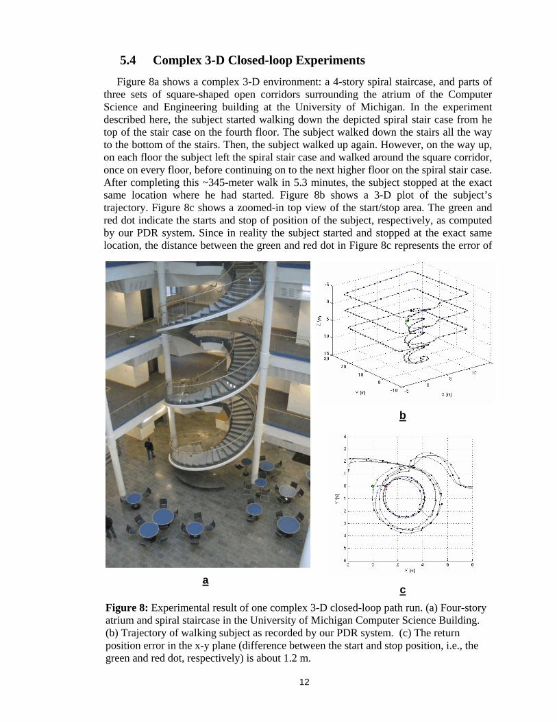
5.4 Complex 3-D Closed-loop Experiments

Figure 8a shows a complex 3-D environment: a 4-story spiral staircase, and parts of three sets of square-shaped open corridors surrounding the atrium of the Computer Science and Engineering building at the University of Michigan. In the experiment described here, the subject started walking down the depicted spiral stair case from he top of the stair case on the fourth floor. The subject walked down the stairs all the way to the bottom of the stairs. Then, the subject walked up again. However, on the way up, on each floor the subject left the spiral stair case and walked around the square corridor, once on every floor, before continuing on to the next higher floor on the spiral stair case. After completing this ~345-meter walk in 5.3 minutes, the subject stopped at the exact same location where he had started. Figure 8b shows a 3-D plot of the subject’s trajectory. Figure 8c shows a zoomed-in top view of the start/stop area. The green and red dot indicate the starts and stop of position of the subject, respectively, as computed by our PDR system. Since in reality the subject started and stopped at the exact same location, the distance between the green and red dot in Figure 8c represents the error of

b

a c

Figure 8: Experimental result of one complex 3-D closed-loop path run. (a) Four-story atrium and spiral staircase in the University of Michigan Computer Science Building. (b) Trajectory of walking subject as recorded by our PDR system. (c) The return position error in the x-y plane (difference between the start and stop position, i.e., the green and red dot, respectively) is about 1.2 m.

13

our system in the x-y plane. In the case here, the error in our three runs averaged about 1.7 m, or 0.5% of the total travel distance of 335 meters. This is especially remarkable in light of the excessive vertical travel, and in light of the fact that the subject’s gait differed significantly in the three modes of walking during this experiment: horizontal walking, as well as climbing up and down the spiral stair case. The error in vertical direction was larger, averaging 4.2 m or 1.2%. Results of these runs are summarized in Table 5 and in Figure 9.

5.5 3-D Closed-loop Experiment on Rugged Terrain

In this experiment we tested our system during the traverse of a rubble pile, about 5 meters high and comprising of chunks of broken concrete and soft soil (see Figure 10a and b). Under these conditions, detecting the footfall is more difficult because of foot slippage and because the key assumption in our ZUPT-based method – zero velocities during ΔT, does not always hold on this terrain. The final positioning error for this experiment was X = 2.0 m and Y = -0.6 m for a total traveled distance of 74.14 m. This amounts to an error of about 2.8% of the traveled distance. We believe we can improve upon this result in the future by using a more effective footfall detection algorithm. We performed only one single run on this terrain, due to logistic limitations.

Figure 9: Position errors in the vicinity of the target point (0, 0) after walking along the complex 3-D closed-loop path.

Table 5: Summary of return position errors for the complex 3-D closed-loop path experiment.

Absolute [m] Relative [%] Event Duration

[min:sec]Distance

[m] X-Y

planeZ-

directionX-Y

planeZ-

direction Walk 1 7:42 358 1.8 4.6 0.50% 1.3% Walk 2 7:36 340 2.1 4.0 0.62% 1.2% Walk 3 7.27 337 1.1 4.1 0.33% 1.2% Average 7:35 345 1.7 4.2 0.49% 1.2%

14

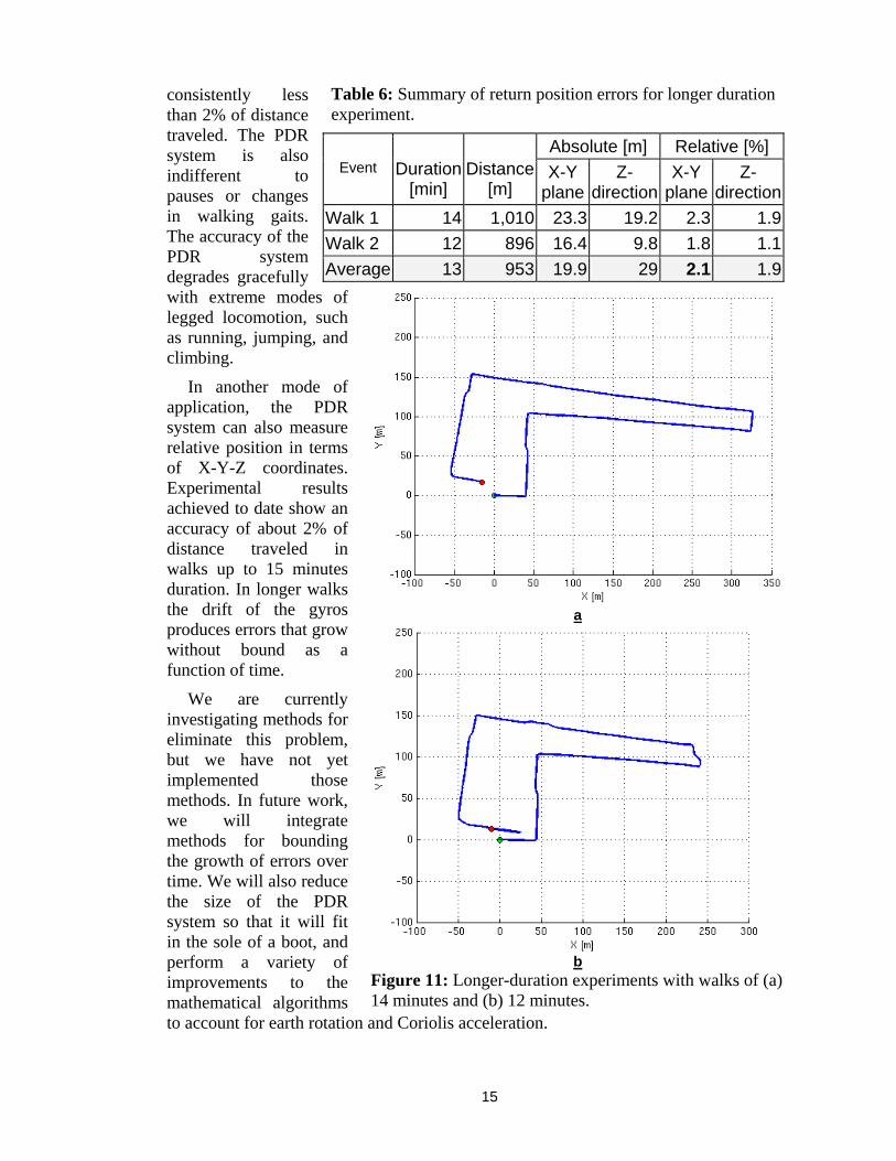
5.6 Longer-duration Experiment

We performed two longer-duration experiments, in which the subject walked for 14 minutes and 12 minutes along mostly horizontal city streets. The travel distances were 1,010 meters and 896 meters, respectively. Figure 11 shows the resulting trajectories and errors, and Table 6 summarized the results.

6 CONCLUSIONS

This paper presented a sophisticated personal dead-reckoning system (PDR system) for emergency responders and security personnel. The PDR system does not require any external references, such as GPS or other pre-positioned fiducials.

The system is very accurate in measuring linear displacements (i.e., distance traveled, a measure similar to that provided by the odometer of a car) with errors being

c

Figure 10: (a) Ruble pile comprising broken-up chunks of concrete and asphalt, as well as dirt; (b) subject climbing up the rubble pile; (c) subject’s trajectory as estimated by the PDR system.

a

b

15

consistently less than 2% of distance traveled. The PDR system is also indifferent to pauses or changes in walking gaits. The accuracy of the PDR system degrades gracefully with extreme modes of legged locomotion, such as running, jumping, and climbing.

In another mode of application, the PDR system can also measure relative position in terms of X-Y-Z coordinates. Experimental results achieved to date show an accuracy of about 2% of distance traveled in walks up to 15 minutes duration. In longer walks the drift of the gyros produces errors that grow without bound as a function of time.

We are currently investigating methods for eliminate this problem, but we have not yet implemented those methods. In future work, we will integrate methods for bounding the growth of errors over time. We will also reduce the size of the PDR system so that it will fit in the sole of a boot, and perform a variety of improvements to the mathematical algorithms to account for earth rotation and Coriolis acceleration.

Table 6: Summary of return position errors for longer duration experiment.

Absolute [m] Relative [%] Event Duration

[min] Distance

[m] X-Y

planeZ-

direction X-Y

plane Z-

directionWalk 1 14 1,010 23.3 19.2 2.3 1.9Walk 2 12 896 16.4 9.8 1.8 1.1Average 13 953 19.9 29 2.1 1.9

a

b

Figure 11: Longer-duration experiments with walks of (a) 14 minutes and (b) 12 minutes.

16

Acknowledgements

This work was funded by the Department of the Army via sub-contract No. S-8844-UM-03 administered by General Dynamics Corporation. Funding was also provided by the U.S. Dept. of Energy under Award No. DE FG52 2004NA25587.

7 BIBLIOGRAPHY

Aoki, H., Schiele, B. and Pentland, A. (1999). “Realtime Personal Positioning System for Wearable Computers.” Proceedings of the International Symposium on Wearable Computers, pp. 37-43. Ayyappa, E. (1997). “Normal Human Locomotion, Part 1: Basic Concepts and Terminology.” Journal of Prosthetics & Orthotics, vol. 9, no. 1, pp. 10-17. Brand, T. And Phillips, R. (2003). “Foot-to-Foot Range Measurement as an Aid to Personal Navigation.” 59th Institute of Navigation Annual Meeting. Albuquerque, NM. Butz, A. Baus, J. And Kruger A. (2000). “Augmenting buildings with infrared information.” Proceedings of the International Symposium on Augmented Reality, IEEE Computer Society Press, pp. 93-96. Cho, S.Y. and Park (C.G., 2006). “MEMS Based Pedestrian Navigation System.” This Journal, vol. 59, pp. 135–153. Galindo, C. et al. (2005). “Vision SLAM in the measurement subspace.” Proceedings of the IEEE International Conf. on Robotics and Automation, Barcelona, Spain, pp. 30-35. Grejner-Brzezinska D. A., Yi Y, and Toth C. K. (2001). “Bridging GPS Gaps in Urban Canyons: Benefits of ZUPT”, Navigation Journal, vol. 48, no. 4, pp. 217-225. Huddle, J. (1998). “Trends in inertial systems technology for high accuracy AUV navigation.” Proceedings of the 1998 Workshop on Autonomous Underwater Vehicles. AUV'98. pp. 63-73. Kourogi M. and Kurata T. (2003). “Personal positioning based on walking locomotion analysis with self-contained sensors and a wearable camera.” Proc. of the Second IEEE and ACM International Symposium on Mixed and Augmented Reality, pp. 103-112. Ledroz, A. et al. (2005). “FOG-based navigation in downhole environment during horizontal drilling utilizing a complete inertial measurement unit: directional measurement-while-drilling surveying.” IEEE Transactions on Instrumentation and Measurement, vol. 54, no. 5, pp. 1997-2006. Liu, Y., Wang, Y., Dayuan Y. And Zhou Y. (2004). “DPSD algorithm for AC magnetic tracking system.” IEEE Symposium on Virtual Environments, Human-Computer Interfaces and Measurement Systems, pp. 101-106. Newman, J., Ingram, D. and Hopper A. (2001). “Augmented reality in a wide area sentient environment.” Proceedings of the IEEE and ACM International Symposium on Augmented Reality, pp. 77-86. Ojeda, L., Chung, H., and Borenstein, J. (2002). "Precision Calibration of Fiber-optics Gyroscopes for Mobile Robot Navigation." Proc. 2000 IEEE International Conference on Robotics and Automation, San Francisco, CA, pp. 2064-2069, April 24-28. PointResearch/Honeywell, (2006), http://pointresearch.com/products.html#DRM, last accessed: 10/2006. Saarinen, J., Suomela, J., Heikkila, Elomaa, M., and Halme, A. (2004). “Personal navigation system.” Proceedings of the 2004 IEEE/RSJ International Conference on Intelligent Robots and Systems, vol 1, pp. 212-217.

17

Savage, P. (1998a). “Strapdown Inertial Navigation Integration Algorithm Design. Part 1: Attitude Algorithms”, Journal of guidance, control, and dynamics, vol. 21, no. 1, pp. 19-28 Savage, P. (1998b). “Strapdown Inertial Navigation Integration Algorithm Design Part 2: Velocity and Position Algorithms”. Journal of Guidance, Control, and Dynamics, vol. 21, no. 2, pp. 208-221. Titerton, D. and Westaon, J. (2004). “Strapdown Inertial Navigation Technology, 2nd Edition.” Progress in Astronautics and Aeronautics Series, Published by AIAA.