Non-Gaussian signatures in Non-Gaussian signatures in cosmic shear fieldscosmic shear fields

Masahiro Takada

(Tohoku U., Japan)

Oct 26th 07 @ ROE

Based on collaboration with

Bhuvnesh Jain (Penn) (MT & Jain 04, MT & Jain 07 in prep.)

Sarah Bridle (UCL) (MT & Bridle 07, astro-ph/0705.0163)

Some part of my talks is based on the discussion of WLWG

Outline of this talkOutline of this talk

• What is cosmic shear tomography?

• Non-Gaussian errors of cosmic shear fields and the higher-order moments

• Parameter forecast including non-Gaussian errors

• Combining WLT and cluster counts

• Summary

Cosmological weak lensing – cosmic shearCosmological weak lensing – cosmic shear

present

z=zs

z=zl

z=0

past

Large-scale structureϕγγϕγγ

γ

2sin

2cos

2

1

=

=+

−=

ba

baobservables

• Arises from total matter clustering– Not affected by galaxy bias uncertainty

– well modeled based on simulations (current accuracy, <10% White & Vale 04)

• A % level effect; needs numerous (~108) galaxies for the precise measurements

Weak Lensing Tomography Weak Lensing Tomography

• Subdivide source galaxies into several bins based on photo-z derived from multi-colors (e.g., Massey etal07)

• <zi> in each bin needs accuracy of ~0.1%

• Adds some ``depth’’ information to lensing – improve cosmological paras (including DE)

＋ m(z)

(e.g., Hu 99, 02, Huterer 01, MT & Jain 04)

Tomographic Lensing Power SpectrumTomographic Lensing Power Spectrum

• Tomography allows to extract redshift evolution of the lensing power spectrum.

• A maximum multipole used should be like l_max<3,000

Tomographic LensiTomographic Lensing Power Spectrum ng Power Spectrum

(contd.)(contd.)

• Lensing PS has a less feature shape, not like CMB– Can’t better constrain inflation parameters (n_s and alp

ha_s) than CMB– Need to use the lensing power spectrum amplitudes t

o do cosmology: the amplitude is sensitive to A_s, de0

(or m0), w(z).

),()(

)(),(00 èL

SS

LLSLLSz

Lm zzd

zdzzddz

S γ ∫∝

Lenisng tomography (condt.)Lenisng tomography (condt.)

• WLT can be a powerful probe of DE energy density and its redshift evolution.• Need 3 z-bins at least, if we want to constrain DE model with 3 parameters (_

de,w0, wa)• Less improvement using more than 4 z-bins, for the 3 parameter DE model

An example of survey parameters An example of survey parameters (on a behalf of HSCWLWG)(on a behalf of HSCWLWG)

• PS measurement error (survey area)^-1• Requirements: expected DE constraints should be comparable wit

h or better than those from other DE surveys in same time scale (DES, Pan-Starrs, WFMOS)

• Note: optimization of survey parameters are being investigated using the existing Suprime-Cam data (also Yamamoto san’s talk)

222

1)12(

2)(⎟⎟⎠

⎞⎜⎜⎝

⎛+

Δ+=⎟⎟

⎠

⎞⎜⎜⎝

⎛

lgskyl

l

CnlflCC εσσ

Area: ~2,000 deg^2

Filters: B~26,V~26,R~26, i’~25.8, z’~24.3

Nights: 150-300 nights

Non-linear clusteringNon-linear clustering

• Most of WL signal is from small angular scales, where the non-linear clustering boosts the lensing signals by an order of magnitude (Jain & Seljak97).

• Large-scale structures in the non-linear stage are non-Gaussian by nature.

• 2pt information is not sufficient; higher-order correlations need to be included to extract all the cosmological information

• Baryonic physics: l>10^3

Non-linear clustering

l_max~3000

Non-Gaussianity induced by structure formationNon-Gaussianity induced by structure formation• Linear regime O()<<1; all the Fourier modes of the

perturbations grow at the same rate; the growth rate D(z)– The linear theory, based on FRW + GR, gives robust, secure predictions

• Mildly non-linear regime O()~1; a mode coupling between different Fourier modes is induced– The perturbation theory gives the specific predictions for a CDM model

• Highly non-linear regime; a more complicated mode coupling– N-body simulation based predictions are needed (e.g., halo model)

)1000()()( == zzDz kk

0)()(

)(),(

)(

4)1()2(2)1(3

21)1()1(

2123

13)2(

)3()2()1(

21

≠∝∝⇒

−−=

+++=

∫∫

kkkkkkk kkk Fdd

z L

,....], ;),([),( LNLbmi zkPfzkP =

• Correlations btw density perturbations of different scales arisCorrelations btw density perturbations of different scales arise as a consequence of non-linear structure formation, originate as a consequence of non-linear structure formation, originating from the initial Gaussian fieldsing from the initial Gaussian fields

• However, the non-Gaussianity is fairly accurately predictable However, the non-Gaussianity is fairly accurately predictable based on the CDM modelbased on the CDM model

Aspects of non-Gaussianity in cosAspects of non-Gaussianity in cosmic shearmic shear

• Cosmic shear observables are non-Gaussian– Including non-Gaussian errors degrades the cosmologic

al constraints?– Realize a more realistic ability to constrain cosmologic

al parameters– The dependences for survey parameters (e.g., shallow s

urvey vs. deep survey)

• Yet, adding the NG information, e.g. carried by the bispectrum, is useful?

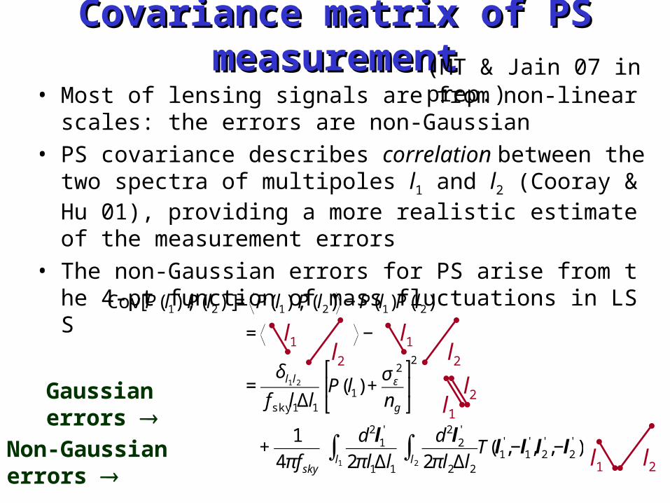
Covariance matrix of PS measurementCovariance matrix of PS measurement

• Most of lensing signals are from non-linear scales: the errors are non-Gaussian

• PS covariance describes correlation between the two spectra of multipoles l1 and l2 (Cooray & Hu 01), providing a more realistic estimate of the measurement errors

• The non-Gaussian errors for PS arise from the 4-pt function of mass fluctuations in LSS

€

Cov[P(l1),P(l2)] = P(l1),P(l2) − P(l1)P(l2)

= −

=δl1l2

fsky l1Δl1P(l1) +

σ ε2

ng

⎡

⎣ ⎢

⎤

⎦ ⎥

2

+1

4πfsky

d2l1'

2πl1Δl1l1∫ d2l2

'

2πl2Δl2l2

∫ T(l1',−l1

',l2' ,−l2

' )

l1l2

l1l2

l2l1

l1 l2

Gaussian errors

Non-Gaussian errors

(MT & Jain 07 in prep.)

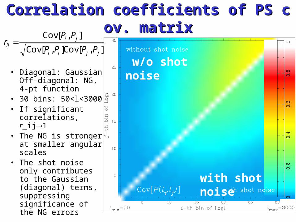
Correlation coefficients of PS cov. matrixCorrelation coefficients of PS cov. matrix

],[Cov],[Cov

],[Cov

jjii

jiij

PPPP

PPr =

• Diagonal: Gaussian Off-diagonal: NG, 4-pt function

• 30 bins: 50<l<3000• If significant

correlations, r_ij1• The NG is stronger at

smaller angular scales• The shot noise only

contributes to the Gaussian (diagonal) terms, suppressing significance of the NG errors

w/o shot noise

with shot noise

Correlations btw Correlations btw Cl’Cl’s at different s at different l’l’ss

• Principal component decomposition of the PS covariance matrix

€

SiaC(li){ } S jbC(l j ){ } = λ aδab

Power spectrum with NG errorsPower spectrum with NG errors

• The band powers btw different ells are highly correlated (also see Kilbinger & Schneider 05)

• NG increases the errors by up to a factor of 2 over a range of l~1000

• ell<100, >10^4, the errors are close to the Gaussian cases

(in z-space as well for WLT)

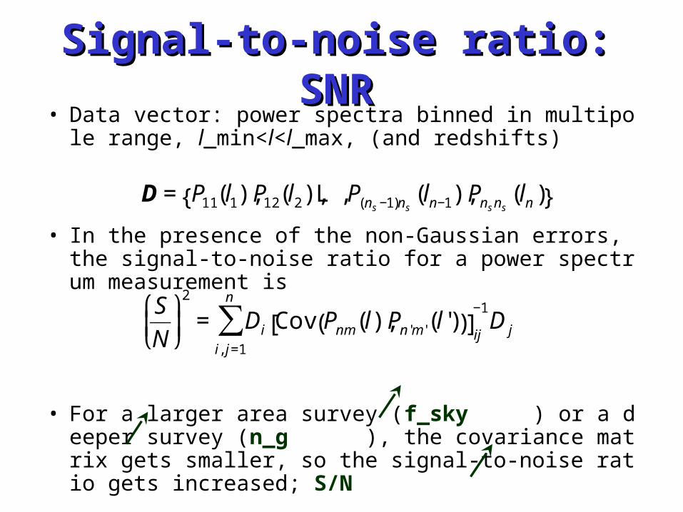
Signal-to-noise ratio: SNRSignal-to-noise ratio: SNR• Data vector: power spectra binned in multipole range, l_

min<l<l_max, (and redshifts)

• In the presence of the non-Gaussian errors, the signal-to-noise ratio for a power spectrum measurement is

• For a larger area survey (f_sky ) or a deeper survey (n_g ), the covariance matrix gets smaller, so the signal-to-noise ratio gets increased; S/N €

S

N

⎛

⎝ ⎜

⎞

⎠ ⎟2

= Di Cov Pnm (l),Pn'm '(l')( )[ ]ij

−1D j

i, j=1

n

∑

€

D = P11(l1),P12(l2),L ,P(ns −1)ns(ln−1),Pns ns

(ln ){ }

Signal-to-noise ratio: SNR (contd.)Signal-to-noise ratio: SNR (contd.)

• Multipole range: 50<l<l_max

• Non-gaussian errors degrade S/N by a factor of 2

• This means that the cosmic shear fields are highly non-Gaussian (Cooray & Hu 01; Kilbinger & Schneider 05)

GaussianNon-Gaussian

50<l<l_max

The impact on cosmo para errorsThe impact on cosmo para errors

_de

w_0

w_a

n_s

….

_mh^2

_bh^2

• We are working in a multi-dimensional parameter space (e.g. 7D)

error ellipse _de

w_0

w_a

n_s

….

_mh^2

_bh^2

Non-Gaussian Error

• Volume of the ellipse: VNG2VG

• Marginalized error on each parameter length of the principal axis: σNG ～ 2^(1/Np)σG (reduced by the dim. of para space)– Each para is degraded by slightly different amounts

– Degeneracy direction is slightly changed

1l2l

3l

1l2l

3l

1l2l

3l

l

An even more direct use of NAn even more direct use of NG: bispectrumG: bispectrum

:)( 22)()()( κκ PWlC GLijji ⇐⇒

:),,( 43321)()()()( κκκ PWB GLijkkji ⇐⇒ lll given as a function of triangles

given as a function of separation l

1l2l

3l

l

1sz2sz

Bernardeau+97, 02, Schneider & Lombardi03, Zaldarriaga & Scoccimarro 03, MT & Jain 04, 07, Kilbinger & Schneider 05

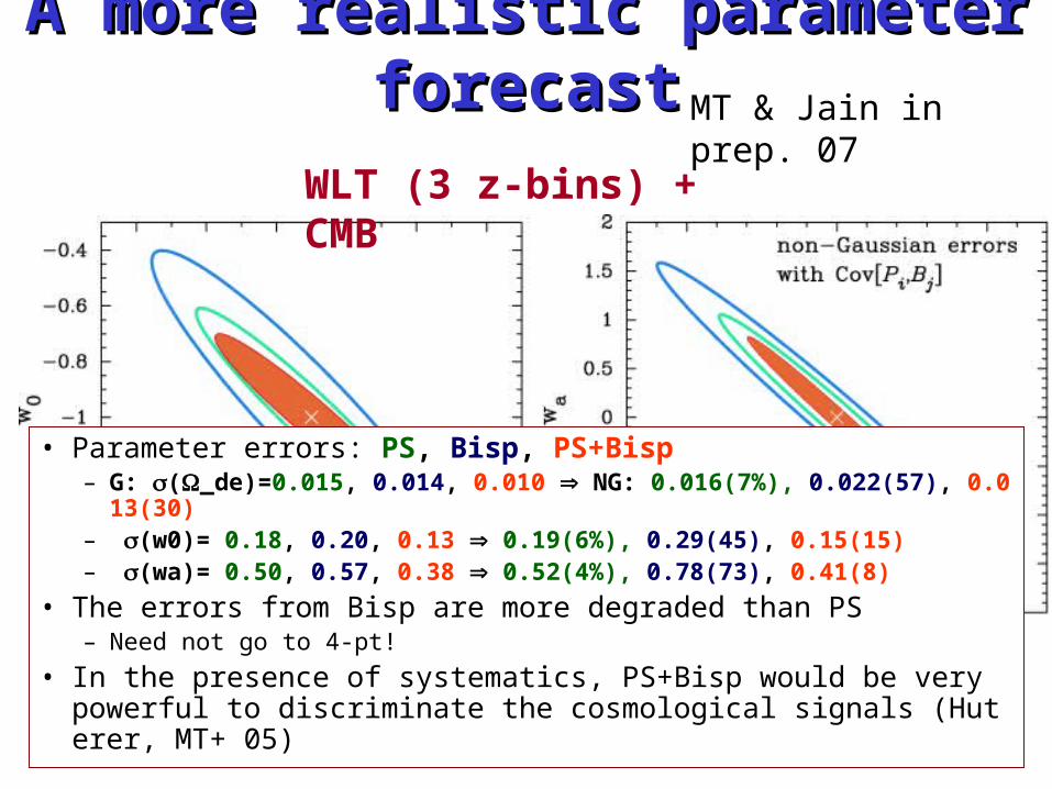
A more realistic parameter forecastA more realistic parameter forecastMT & Jain in prep. 07

WLT (3 z-bins) + CMB

• Parameter errors: PS, Bisp, PS+Bisp – G: σ(_de)=0.015, 0.014, 0.010 NG: 0.016(7%), 0.022(57), 0.013(30) – σ(w0)= 0.18, 0.20, 0.13 0.19(6%), 0.29(45), 0.15(15) – σ(wa)= 0.50, 0.57, 0.38 0.52(4%), 0.78(73), 0.41(8)

• The errors from Bisp are more degraded than PS– Need not go to 4-pt!

• In the presence of systematics, PS+Bisp would be very powerful to discriminate the cosmological signals (Huterer, MT+ 05)

WLT + Cluster CountsWLT + Cluster Counts

• Clusters are easy to find from WL survey itself: mass peaks (Miyazaki etal.03; see Hamana san’s talk for the details)

• Synergy with other wavelength surveys (SZ, X-ray…) – Combining WL signal and other data is very useful to discriminate real clu

sters from contaminations

• Combing WL with cluster counts is useful for cosmology?– Yes, would improve parameter constraints, but how complementary?

• Cluster counts is a powerful probe of cosmology, established method (e.g., Kitayama & Suto 97)

MT & S. Bridle astro-ph/0705.0163

)obs;()( 2

cl mSmndmdzd

VddzN ∫∫

=Angular number counts:

w0=-1 w0=-0.9

Mass-limited cluster counts vs. lenMass-limited cluster counts vs. lensing-selected countssing-selected counts

• Mass-selected sample (SZ) vs lensing-based sample

Halo distribution Convergence map

Hamana, MT, Yoshida 04

2 d

egre

es

Miyazaki, Hamana+07

QuickTime˛ Ç∆TIFFÅià≥èkǻǵÅj êLí£ÉvÉçÉOÉâÉÄ

ǙDZÇÃÉsÉNÉ`ÉÉÇ å©ÇÈÇΩÇflÇ…ÇÕïKóvÇ≈Ç∑ÅB

Mass

Light (galaxies)

X-ray

Secure candidates

A closer look at nearby clusters (z<0.3)A closer look at nearby clusters (z<0.3)

QuickTime˛ Ç∆TIFFÅià≥èkǻǵÅj êLí£ÉvÉçÉOÉâÉÄ

ǙDZÇÃÉsÉNÉ`ÉÉÇ å©ÇÈÇΩÇflÇ…ÇÕïKóvÇ≈Ç∑ÅB

~30 clusters (Okabe, MT, Umetsu+ in prep.)

• Subaru is superb for WL measurement• A detailed study of cluster physics (e.g. the nature of dark matter)

Redshift distribution of cluster samplesRedshift distribution of cluster samples

Cross-correlation between CC and WLCross-correlation between CC and WL

• If the two observables are drawn from the same survey region, the two probe the same cosmic mass density field in LSS

• Around each cluster, stronger shear signal is expected: up to ~10% in induced ellipticities, compared to a few % for typical cosmic shear

• A positive cross-correlation is expected: Clusters happen to be less/more populated in a given survey region than expected, the amplitudes of <γγ> are most likely to be smaller/greater

• Note that < γγ >: 2pt, cluster counts (CC): 1pt =>no correlation for Gaussian fields

A patch of the observed sky

Cluster

Shearing effect on background galaxies

Cross-correlation btw CC and WL (contd.)Cross-correlation btw CC and WL (contd.)

• Shown is the halo model prediction for the lensing power spectrum

• A correlation between the number of clusters and the ps amplitude at l~10^3 is expected.

M/M_s>10^14

M/M_s>10^13

M/M_s>10^15

Cross-covariance between CC + WLCross-covariance between CC + WL• Cross-covariance between PS binned in l and z and the cluster c

ounts binned in z

• The cross-correlation arises from the 3-pt function of the cluster distribution and the two lensing fields of background galaxies– The cross-covariance is from the non-Gaussianity of LSS

• The structure formation model gives specific predictions for the cross-covariance

SNR for SNR for CC+WLCC+WL

• The cross-covariance leads to degradation and improvement in S/N up to ~20%, compared to the case that the two are independent

Parameter forecasts for CC+WLParameter forecasts for CC+WL

• Lensing-selected sample with detection threshold S/N~10 contains clusters with >10^15Msun

• Lensing-selected sample is more complementary to WLT, than a mass-selected one? Needs to be more carefully addressed

lensing-selected sample mass-selected sample

WLCC+WLCC+WL with Cov

HSCWLS performance (WLT+CC+CMBHSCWLS performance (WLT+CC+CMB) )

• Combining WLT and CC does tighten the DE constraints, due to their different cosmological dependences

• Cross-correlation between WLT and CC is negligible; the two are considered independent approximately

Real world: issues on systematic errorsReal world: issues on systematic errors• E/B mode separation as a diagnostics of systematics• Non-gaussian signals in weak lensing fields• Theoretical compelling theoretical modeling of DE• Shape measurement accuracies vs. galaxy types, morphology, magnitudes…• Data reduction pipelines optimized for weak lensing analyses• Exploring a possibility to self-calibrate systemtaics, by combining different methods• Non-linearities in lensing; reduced shear needs to be included?• Intrinsic alignments• Source clustering, source-lens coupling• Usefulness of Flexions?• Develop a sophisticated photo-z code• Photo-z vs. color space? • Requirement on spec-z sub-sample; from which data?• N-body simulations (initial conditions, how to work in multi-dimenaional parameter space for N-body simulations, the

strategy…)• DE vs. modified gravity• Fourier space vs. real-space; explore an optimal method to measure power spectrum from actual data, with complex su

rvey geometry• Exploring a code of likelihood surface in a multi-dimensional parameter space (MCMC); how to combine with other p

robes such as CMB, 2dF/SDSS, ….• Can measure DE clustering or neutrino mass from WL or else with HSC?• Defining survey geometry: a given total survey area, many small-patched survey regions vs. continuous survey region• Adding multi-color info for WL based cluster finding; color properties of member ellipticals would be useful to discri

minate real lensing mass peaks as well as know the redshift • How to calibrate mass-observable relation for cluster experiments? WL + colors + SZ + X-ray?• Constraining mass distribution within a cluster with HSC WL survey; mass profile, halo shape, etc• Strong lens statistics• Imaging BAO• Man power problem: who and when to work on these issues? • …

Issues on systematics: self-calibrationIssues on systematics: self-calibration

,..... , 222111 jjjiii SCOSCO +=+=

jijiji CCOOOO 212121 ],[Cov ==

• If several observables (O1,O2,…) are drawn from the same survey region: e.g., WLPS, WLBisp, CC,…– Each observable contains two contributions (C: cosmological signal and

S: systematics)

• Covariances (or correlation) between the different obs.– If the systematics in different obs are uncorrelated

– The cosmological covariances are fairly accurately predictable

• Taking into account the covariances in the analysis could allow to discriminate the cosmological signals from the systemacs – self-calibration– Working in progress

SummarySummary• The non-Gaussian errors in cosmic shear fields arise from non

-linear clustering in structure formation– The CDM model provides the specific predictions, so the NG errors ar

e in some sense accurately predictable

• Bad news: the NG errors are very important to be included for current and, definitely, future surveys– The NG degrades the S/N for the lensing power spectrum measuremen

t up to a factor of 2

• Good news: the NG impact on cosmo para errors are less significant if working in a multi-dimensional parameter space– ~10% for 7-D parameter space

• WLT and cluster counts, both available from the same imaging survey, can be used to tighten the cosmological constraints