NON-GAUSSIAN 4D VAR STEVEN J. FLETCHER and MANAJIT SENGUPTA · NON-GAUSSIAN 4D VAR STEVEN J....

NON-GAUSSIAN 4D VAR

STEVEN J. FLETCHER and MANAJIT SENGUPTA

With thanks to Milija and Dusanka Zupanski, Andy Jones, Laura Fowlerand Thomas Vonder Haarand Thomas Vonder Haar

DoD Center for Geosciences/Atmospheric Research (CG/AR)p ( )

COOPERATIVE INSTITUTE FOR RESEARCH IN THE ATMOSPHERE

COLORADO STATE UNIVERSITY

CSU/CIRA Steven J. Fletcher 8th Adjoint Workshop, May 21st 2009 1

PRESENTATION OUTLINE

MOTIVATION FOR THE WORK

REAL LIFE EXAMPLES OF NON-GAUSSIAN VARIABLES

MATHEMATICAL ILLUSTRATIONS OF THE DRAWBACKS OF CURRENT METHODSMETHODS

PROBABILISTIC APPROACH USING CONDITIONAL INDEPENDENCE

4 D HYBRID LOGNORMAL NORMAL DATA ASSIMILATION4-D HYBRID LOGNORMAL – NORMAL DATA ASSIMILATION


MOTIVATION

An important assumption made in variational and ensemble data assimilation is that the state variables and observations are Gaussianassimilation is that the state variables and observations are Gaussian distributed

Note: The difference between two Gaussian variables is also a Gaussian variable.

Is this true for all state variables?

Is this true for all observations of the atmosphere?


REAL LIFE EXAMPLES

This data is column water vapour climatologies from the Oklahoma ARM-SGP site from 1997-2000 where the data are of when a boundary layer cloud was presentcloud was present

We have taken the observations and have sorted them by season as well as for the whole year. The data was collected using a microwave radiometer.


1

BEST LOGNORMAL AND NORMAL FITS FOR CWV FOR DJF

CWV DJFBEST LOGNORMAL FITBEST NORMAL FIT

0.6

0.8

sity

BEST LOGNORMAL AND NORMAL FITS FOR CWV FOR MAM

CWV MAM

0.4

0.6

Den

si

0.4

0.5

CWV MAMBEST LOGNORMAL FITBEST NORMAL FIT

1 2 3 4 5 60

0.2

0.3

0.4

Den

sity

1 2 3 4 5 6COLUMN WATER VAPOR

0.2

De

1 2 3 4 5 60

0.1

COLUMN WATER VAPOR


1 2 3 4 5 6COLUMN WATER VAPOR

0.35

0.4

0.45

BEST LOGNORMAL AND NORMAL FITS FOR CWV FOR JJA

0.25

0.3

0.35

ensi

ty

0.1

0.15

0.2Den

CWP JJA

BEST LOGNORMAL FIT BEST LOGNORMAL AND NORMAL FITS FOR CWV FOR SON

1.5 2 2.5 3 3.5 4 4.5 5 5.5 60

0.05

COLUMN WATER VAPOR

BEST LOGNORMAL FIT

BEST NORMAL FIT

0.35

0.4

BEST LOGNORMAL AND NORMAL FITS FOR CWV FOR SON

CWV SONBEST LOGNORMAL FITBEST NORMAL FIT

0.2

0.25

0.3en

sity

0.1

0.15

0.2Den

CSU/CIRA Steven J. Fletcher 8th Adjoint Workshop, May 21st 2009 61 2 3 4 5 60

0.05

COLUMN WATER VAPOR

BEST LOGNORMAL AND NORMAL FITS FOR CWV FOR ALL SEASONS

0.4

0.45

BEST LOGNORMAL AND NORMAL FITS FOR CWV FOR ALL SEASONS

CWV ALL SEASONSBEST LOGNORMAL FITBEST NORMAL FIT

0.25

0.3

0.35

sity

0.15

0.2

0.25

Den

sit

0.05

0.1

1 2 3 4 5 60

COLUMN WATER VAPOR


Current Techniques used with non-Gaussian Variables

1) Transform by taking the LOGARITHM of the original state variable. This then makes the new variable ALMOST GAUSSIAN. Minimize the cost function with respect to this variable, TRANSFORM BACK and initialize with this state. STATE FOUND IS A NON-UNIQUE MEDIAN OF THE ORIGINAL VARIABLE, (Fletcher and Zupanski 2006a, 2007).

2) Assumed Gaussian assumption and BIAS CORRECT2) Assumed Gaussian assumption and BIAS CORRECT.

3) Using a Markov-Chain Monte-Carlo approaches (Posselt et al. 2008)


1.8PLOT OF LOGNORMAL DISTRIBUTIONS

σ=0.25

1.4

1.6σ=0.25σ=0.5σ=1σ=1.5

1

1.2

DF

=1.5

0.6

0.8PD

F

0.2

0.4

0.6

0 0.5 1 1.5 2 2.5 30

0.2

x


x

1.8PLOT OF TRANSFORMED NORMAL DISTRIBUTIONS

σ=0.25

1.4

1.6σ=0.25σ=0.5σ=1σ=1.5

1

1.2

DF

0.6

0.8PD

F

0.2

0.4

0.6

−2 −1.5 −1 −0.5 0 0.5 1 1.5 20

0.2

ln x


ln x

1.8PLOT OF LOGNORMAL DISTRIBUTIONS

1.8PLOT OF TRANSFORMED NORMAL DISTRIBUTIONS

1.4

1.6

1.8σ=0.25σ=0.5σ=1σ=1.51.4

1.6

1.8σ=0.25σ=0.5σ=1σ=1.5

0.8

1

1.2

PD

F

0.8

1

1.2

PD

F

0.2

0.4

0.6

0.2

0.4

0.6

0 0.5 1 1.5 2 2.5 30

0.2

x−2 −1.5 −1 −0.5 0 0.5 1 1.5 20

0.2

ln x

All skewness information is lost


0.2

0.22

0.24

RANDOM LOGNORMAL SAMPLE WITH μ=0, σ=0.5, SAMPLE=20,000

a) FIRST SAMPLELOGNORMAL BEST FIT 0.16

0.18

RANDOM LOGNORMAL SAMPLE WITH μ=0, σ=1, SAMPLE=20,000

b) SECOND SAMPLELOGNORMAL BEST FIT

0.1

0.12

0.14

0.16

0.18

0.2

PD

F

0.08

0.1

0.12

0.14

PD

F

0.02

0.04

0.06

0.08

0.1

0.02

0.04

0.06

0.08

0 1 2 3 4 5 60

0.02

X0 1 2 3 4 5 6 7 8 9 10

0

X

0.12DIFFERENCE BETWEEM THE TWO LOGNORMAL SAMPLES

d)DIFFERENCES

0.06

0.08

0.1

DF

DIFFERENCES

NOTE: DIFFERNCE IS NOT

ASSUMED GAUSSIAN APPROACH

0.02

0.04

0.06

PD

A GAUSSIAN


−10 −8 −6 −4 −2 0 2 40

X

0.2

0.22

0.24RANDOM LOGNORMAL SAMPLE WITH μ=0, σ=0.5, SAMPLE=20,000

a) FIRST SAMPLELOGNORMAL BEST FIT

0.07

0.08

0.09RANDOM LOGNORMAL SAMPLE WITH μ=1, σ=0.5, SAMPLE=20,000

b) SECOND SAMPLELOGNORMAL BEST FIT

0.1

0.12

0.14

0.16

0.18

PD

F

0.04

0.05

0.06

0.07

PD

F

0.02

0.04

0.06

0.08

0.1

0.01

0.02

0.03

0 1 2 3 4 5 60

0.02

X

0 1 2 3 4 5 6 7 8 9 100

X

0.07

0.08DIFFERENCE BETWEEM THE TWO LOGNORMAL SAMPLES

d) DIFFERENCES

0.04

0.05

0.06

0.07

DF

NOTE: DIFFERNCE IS NOT

0.02

0.03

0.04

PD

F

A GAUSSIAN

CSU/CIRA Steven J. Fletcher 8th Adjoint Workshop, May 21st 2009 13−10 −9 −8 −7 −6 −5 −4 −3 −2 −1 0 1 2 3 4 50

0.01

X

PROBLEMS ASSOCIATED WITH CURRENT TECHNIQUESQ

ASSUMED GAUSSIAN:

IMPACT 1: Wrong probabilities assigned to outliers.

IMPACT 2: Probabilities assigned to unphysical values.

IMPACT 3: Wrong statistic used to approximate the true distribution of the random variable.


MISCONCEPTIONS ABOUT LOGNORMAL DATAMISCONCEPTIONS ABOUT LOGNORMAL DATA ASSIMILATION

1) The theor holds as the backgro nd sol tion is independent of the tr e1) The theory holds as the background solution is independent of the true solution, it is only an approximation and statistically has no information about the true solution.

2) The theory holds for the observational component as the observations are independent of the observations operator and vice-versa.

3) If two solutions have a relative error of 50% then we are still out by a factor of two in both cases no matter what order of magnitude.


4D LOGNORMAL DATA ASSIMILATIONUnlike with the three dimensional version of variational data assimilation, the four dimensional version is defined as a weighted least squares problem.

Th G i i ht d l t h t 4D VARThe Gaussian weighted least squares approach to 4D VAR is defined through a calculus of variation problem with initial conditions found through the adjoint.

This weighted least squares approach can be defined for aThis weighted least squares approach can be defined for a lognormal framework, which is defined by the following inner product

N

( ) ( )( ) ( )( )( )∫∫∫∑=

− −−=A

N

iiiiiiii

o

g1

01

01 lnln,lnln21 xMhyRxMhyx0


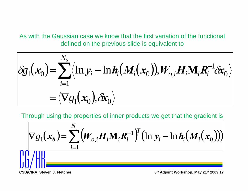
As with the Gaussian case we know that the first variation of the functionalAs with the Gaussian case we know that the first variation of the functional defined on the previous slide is equivalent to

0N

( ) ( )( )1

01

,001 ,lnln0

xRHWxMhyx δδgN

iiiiioiii −=∑

=

−M

( ) 001

1

, xx δgi

∇==

Through using the properties of inner products we get that the gradient is

( ) ( ) ( )( )( )1N

To

∑( ) ( ) ( )( )( )01

1,1 lnln xMhyRHWx0 iii

i

Tiiiiog −=∇ ∑

=

−M


The solution is a median and not the mode and hence is independent of the variance.

We need to define the functional as

( ) =g x( )

( )( ) ( )( )( )∫∫∫∑ − −+−

=N

iiiiT

iii

o

g

01

0

2

lnln,lnln21 xMhyR1RxMhy

x0

( )( ) ( )( )( )∫∫∫∑=A i

iiiiiii1

00 ,2

yy

Which then has a gradient of

( ) ( ) ( )( )( )1RxMhyRHWx T+∇ ∑ −1 lnlnN

To

g M

Which then has a gradient of

( ) ( ) ( )( )( )1RxMhyRHWx i0 +−=∇ ∑=

01

,2 lnln iiii

iiiiog M


Current Gaussian approachN

I d T f t h i

( ) ( )( )( ) ( )( )( )∑=

− −−=0

10,00,0

1,0 ,

N

iiiiiiiiGG MMJ xhyxhyRx

Improved Transform technique

( ) ( )( )( )( ) ( )( )( )( )∑ − −−=0

0,00,01,0 lnln,lnln

N

iiiiiiiLTR MMJ xhyxhyRx

New Lognormal 4D VAR approach:

( ) ( )( )( )( ) ( )( )( )( )∑=1

,,,i

( ) ( )( )( )( ) ( )( )( )( )∑=

− −+−=0

1,01

0,0,0,01,0 lnln,lnln

N

iiiiNiLiiiiLLN MMJ xhy1RxhyRx

Term that gives the mode


PROBABILITY APPROACH


( )N321N210 y,,y,y,yx,,x,x,x0

KK =Po

( ) ( ) ( ) ( )( )

0112011010 x,xyxx,xyxxx0

PPPPo

,

( )011N1NNN x,x,y,,x,y,xyooKK −oP

The expression above is Bayes theorem for a multi-event probability situation. It can be simplified through using conditional independence.

( ) ( ) ( )∏=oN

PPP xyxyyyyxxxx( ) ( ) ( )∏=

=o

iiPPP

100N321N210 xyxy,,y,y,yx,,x,x,x

0KK


Taking the negative logarithm of the circled pdf in the previousTaking the negative logarithm of the circled pdf in the previous slide results in

⎫⎧ N

( ) ( ) ( )⎭⎬⎫

⎩⎨⎧

−−= ∑=

0

1000 lnlnmin

N

iiPPJ xyxx

This can now be used to derive a 4D VAR system for any distributed random variable


( )( )( )

=

∏

N321N210 y,,y,y,yx,,x,x,x0

N

P

o

oKK

( ) ( )=∏ 00 xyxi

iPP1

hG il i iF h

( ) ( ) ( )⎭⎬⎫

⎩⎨⎧ −−−∝ −

b 00b 000 xxBxxx TP 10

1exp

havewecaseGaussian temultivaria For the

( ) ( ) ( )

( ) ( )( )( ) ( )( )( )⎬⎫⎨⎧ −−−∝

⎭⎬

⎩⎨∝

−

b,00b,000

xMhyRxMhyxy

xxBxxx

TP

P

1

0

1exp

2exp

( ) ( )( )( ) ( )( )( )⎭⎬

⎩⎨ −−−∝ 0i0i0 xMhyRxMhyxy iiiiiiP

2exp


( ) ⎟⎞

⎜⎛∏ i0,x

N

P

havewecaselognormaltemultivariaFor the

( )

( ) ( )⎫⎧

×⎟⎟⎠

⎜⎜⎝

∝=∏

jb,0,

i0,0 xx

T

j

P

1

1

1 ( ) ( )

( )( )⎟⎞⎜⎛

⎭⎬⎫

⎩⎨⎧ −−− −

b,00b,00

xM

xxBxx

N

T

io h

10 lnlnlnln

21exp

,

( ) ( )( )

⎫⎧

×⎟⎟⎠

⎞⎜⎜⎝

⎛∝

=∏0

xMxy

k ki

kii y

hP

1 ,

0,,

( )( )( ) ( )( )( )⎭⎬⎫

⎩⎨⎧ −−− −

0i0i xMhyRxMhy iiiT

ii1

21exp


Results with the Lorenz 1963 modelResults with the Lorenz 1963 model


We are going to be using the hybrid Gaussian-lognormal distribution andWe are going to be using the hybrid Gaussian lognormal distribution and comparing it with the transform approach. The associated cost function is

( ) ( ) ⎞⎛T1 0( ) ( ) ( ) ⎟⎠

⎞⎜⎝

⎛+−−= −

NN

qb

pbTbb

Tb

Tb

TbJ

,

,102

110

εεεBεεx

( ) ( ) ⎟⎠

⎞⎜⎝

⎛+−−+ ∑∑

==

−

iqo

ipoN

i

Tioio

Tio

N

ii

Tio

Tio

oo

,,

,,

1,,,

1

1,, 1

0εεεRεε

ii 11

( )( )⎟

⎞⎜⎛ −

=⎟⎟⎞

⎜⎜⎛ −

= hxhy

εxx

ε ipipi

pbpb

,,,llll

1

( )⎟⎠⎜⎝ −⎟⎟

⎠⎜⎜⎝ − xhyεxxε o

iqiqi

qbqb

,,,

, lnlnlnln1


Example with the Lorenz 1963 model

The three non-linear differential equations are given by (Lorenz 1963)

yxx σσ +−=&28AND108β

zxyzyxxzy

y

βρ

=−+−=

&

&28AND10,

3=== ρσβ

zxyz β−=

5606.22 AND 4841.5,4458.5 000 =−=−= zyx

Going to assume x and y components and the associated obs are Gaussian z is lognormalGaussian, z is lognormal

(Fletcher and Zupanski 2007)


Plots of the differences in the trajectories with manytrajectories with many

accurate obs with short assimilation windows

Note transform andNote: transform and hybrid approach

quite similar

BEST CASE SCENERIO


SCENERIO

When assimilation window is l (1000t ) ith f dlarge (1000ts) with fewer and

less accurate obs, hybrid approach is more accurate

Transform approach converges quickly toconverges quickly to the wrong solution


Conclusions and Further WorkCareful which statistic to use to analyses yMode is closer to the true trajectory in the Lorenz 63 modelPossible to assimilate variables of mixed types simultaneously Combine other distributions?? i.e. Gamma, Normal, LognormalMore consistent methods for finding positive definite variablesN d t h b k d i t i (if l dNo need to change background error covariance matrix (if already

using the transform approach)


NON-GAUSSIAN 4D VAR STEVEN J. FLETCHER and MANAJIT SENGUPTA · NON-GAUSSIAN 4D VAR STEVEN J....

Documents

Transcript of NON-GAUSSIAN 4D VAR STEVEN J. FLETCHER and MANAJIT SENGUPTA · NON-GAUSSIAN 4D VAR STEVEN J....