ROCKIN’ IT FOR JESUS!. Nothing, nothing, Absolutely nothing! Nothing, nothing, Absolutely nothing!
Upload
ethel-woodCategory
view
230download
0
(Non) Equilibrium Selection, (Non) Equilibrium Selection, Similarity Judgments and the Similarity Judgments and the
“Nothing to Gain / Nothing to Lose” “Nothing to Gain / Nothing to Lose” EffectEffect
Jonathan W. LelandJonathan W. LelandThe National Science Foundation*The National Science Foundation*
June 2007June 2007*The research discussed here was funded by an Italian *The research discussed here was funded by an Italian
Ministry of Education “Ministry of Education “Rientro dei Cervelli” fellowship. Rientro dei Cervelli” fellowship. Views expressed do not necessarily represent the views the Views expressed do not necessarily represent the views the
National Science Foundation nor the United States National Science Foundation nor the United States government. Not for quote without permissiongovernment. Not for quote without permission

MotivationMotivation
““Many interesting games have Many interesting games have more than one Nash equilibrium. more than one Nash equilibrium. Predicting which of these Predicting which of these equilibria will be selected is equilibria will be selected is perhaps the most important perhaps the most important problem in behavioral game problem in behavioral game theory.” (Camerer, 2003)theory.” (Camerer, 2003)
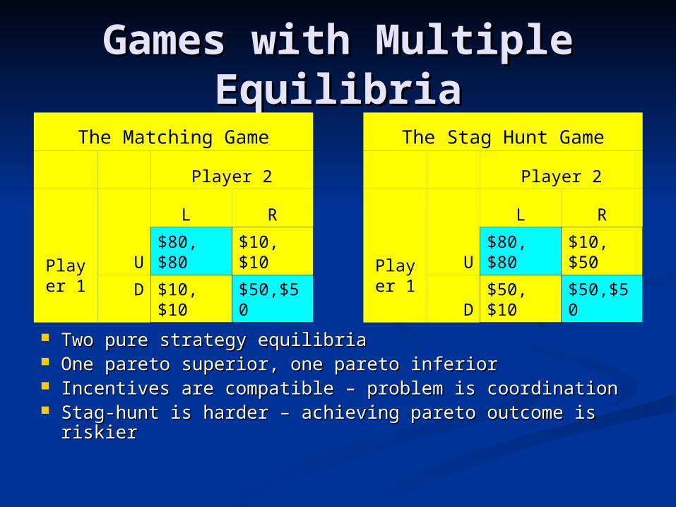
Games with Multiple Games with Multiple EquilibriaEquilibria
Two pure strategy equilibriaTwo pure strategy equilibria One pareto superior, one pareto inferiorOne pareto superior, one pareto inferior Incentives are compatible – problem is coordinationIncentives are compatible – problem is coordination Stag-hunt is harder – achieving pareto outcome is Stag-hunt is harder – achieving pareto outcome is
riskierriskier
The Matching Game The Stag Hunt Game
Player 2 Player 2
L R L R
Player 1
U $80, $80 $10, $10 Player 1
U $80, $80 $10, $50
D$10, $10 $50,$50 D $50, $10 $50,$50

Equilibrium Selection Equilibrium Selection CriteriaCriteria
Payoff DominancePayoff Dominance choose choose the equilibriumthe equilibrium offering all players their offering all players their highest payoffhighest payoff – predicts UL – predicts UL
Security-mindedness Security-mindedness choose choose the strategythe strategy that that minimizes the worst possible payoff – predicts DRminimizes the worst possible payoff – predicts DR
Risk DominanceRisk Dominance choose the strategy that minimizes loses choose the strategy that minimizes loses
incurred by players as a consequence of incurred by players as a consequence of unilaterally deviating from their eq. strategy – unilaterally deviating from their eq. strategy – predicts DRpredicts DR
The Stag Hunt Game
Player 2
L R
Player 1
U $8, $8 $1, $5
D $5, $1 $5,$5

An Alternative Approach An Alternative Approach Similarity Judgments in ChoiceSimilarity Judgments in Choice
R:{$XR:{$X ,, pp ;; $Y$Y ,, 1-p1-p } } S:{$MS:{$M,, qq ;; $N$N ,, 1-q1-q }}
Choose R (S) if it is favored in some Choose R (S) if it is favored in some comparisons and not disfavored in any, comparisons and not disfavored in any, otherwise choose at random.otherwise choose at random.
X similar / X similar / dissimilar Mdissimilar M
p similar / p similar / dissimilar qdissimilar q
Y similar / Y similar / dissimilar dissimilar
NNFavor R, Favor S,
Inconclusive, Inconsequential
Favor R, Favor S,
Inconclusive, Inconsequenti
al
1-p similar / 1-p similar / dissimilar 1-dissimilar 1-

Similarity Judgments Similarity Judgments The “Nothing to Gain/Nothing to Lose” The “Nothing to Gain/Nothing to Lose”
EffectEffectR:{$10R:{$10 ,, .90.90 ;; $0$0 ,, .10.10
} }
S:{$9S:{$9 ,, .90.90 ;; $9$9 ,, .10.10 }}
R’:{$10R’:{$10 ,, .10.10 ;; $0$0 ,, .90.90} }
S’:{$1S’:{$1 ,, .10.10 ;; $1$1 ,, .90.90 }}
10 ~10 ~xx 9 9 .90 ~ .90 ~ pp .90 .90 9 >9 >xx 0 0
.90 ~.90 ~pp .90 .90
Inconsequential Favors S
ntgntg
10 >10 >xx 1 1 .10 ~ .10 ~ pp .10 .10
Favors R’
1 ~1 ~xx 0 0
.10 ~ .10 ~ pp .10 .10
Inconsequential
ntlntl
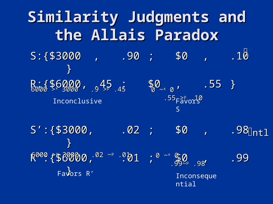
Similarity Judgments and Similarity Judgments and the Allais Paradoxthe Allais Paradox
S:{$3000S:{$3000 ,, .90.90 ;; $0$0 ,, .10.10} }
R:{$6000,R:{$6000, .45.45 ;; $0$0 ,, .55.55 }}
S’:{$3000,S’:{$3000, .02.02 ;; $0$0 ,, .98.98 } }
R’:{$6000,R’:{$6000, .01.01 ;; $0$0 ,, .99.99 } }
6000 >6000 >xx 3000 .9 > 3000 .9 >pp .45 .45 0 ~0 ~xx 0 .55 > 0 .55 >pp .10 .10 Inconclusive Favors
S
Favors R’ Inconsequential
ntlntl
6000 >6000 >xx 3000 .02 ~ 3000 .02 ~pp .01 .01 0 ~0 ~xx 0 .99~0 .99~pp .98 .98

Similarity Judgments and Similarity Judgments and Intertemporal ChoiceIntertemporal Choice
T1:{$20,T1:{$20, 1 month1 month }}
T2:{$25T2:{$25 ,, 2 months2 months }}
T11:{$20,T11:{$20, 11 month11 month }}
T12:{$25T12:{$25 ,, 12 months12 months }}
S or D?$25 >$25 >xx $20 $20
S or D?2 >2 >tt 1 1 Inconclusi
ve Choose either
Nothing to lose Choose T12
S or D?$25 >$25 >xx $20 $20
S or D?12 ~12 ~tt 11 11

Sources of prediction in Sources of prediction in Similarity based modelsSimilarity based models
Intransitivity of the similarity relation Intransitivity of the similarity relation E.g., 20 ~E.g., 20 ~xx 17, 17 ~ 17, 17 ~xx 15 but 20 > 15 but 20 >xx 15 15 Theoretically inconsequential manipulation of Theoretically inconsequential manipulation of
prizes, probabilities, dates of receipt may have prizes, probabilities, dates of receipt may have consequences if they influence perceived consequences if they influence perceived similarity or dissimilarity.similarity or dissimilarity.
Framing of the choiceFraming of the choice Framing determines what is compared with Framing determines what is compared with
what – theoretically inconsequential changes what – theoretically inconsequential changes in the description of the choice may influence in the description of the choice may influence what is compared with what. what is compared with what.

Application to Games - Application to Games - PreliminariesPreliminaries
AssumeAssume Players all have the same Bernoullian Players all have the same Bernoullian
utility functionutility function Let:Let:
>>xx mean “is dissimilar and greater than” mean “is dissimilar and greater than” A strict partial order (asymmetric and A strict partial order (asymmetric and
transitive)transitive) ~~xx mean “is similar to” mean “is similar to”
Symmetric but not necessarily transitive (e.g., Symmetric but not necessarily transitive (e.g., 20 ~20 ~xx 15, 15 ~ 15, 15 ~xx 10 but 20 > 10 but 20 >xx10.10.

Similarity Judgments in Similarity Judgments in GamesGames
L R
U h, t l, c
D m, b m, c
Player 2
Player 1
L R
U 8, 8 2, 5
D 5, 2 5, 5
Player 2
Player 1
Payoffs to Player 1: h(igh) > m(edium) > l(ow)Payoffs to Player 1: h(igh) > m(edium) > l(ow) Payoffs to Player 2: t(op) > c(enter) > b(ottom)Payoffs to Player 2: t(op) > c(enter) > b(ottom) Decision processDecision process
Do I have a dominating strategy, if so, choose it.Do I have a dominating strategy, if so, choose it. Do I have dominating strategy in similarity – if so, choose it.Do I have dominating strategy in similarity – if so, choose it. Does Other have dominating strategy, if so, best respondDoes Other have dominating strategy, if so, best respond Does Other have dominating strategy in similarity, if so, best respondDoes Other have dominating strategy in similarity, if so, best respond ??
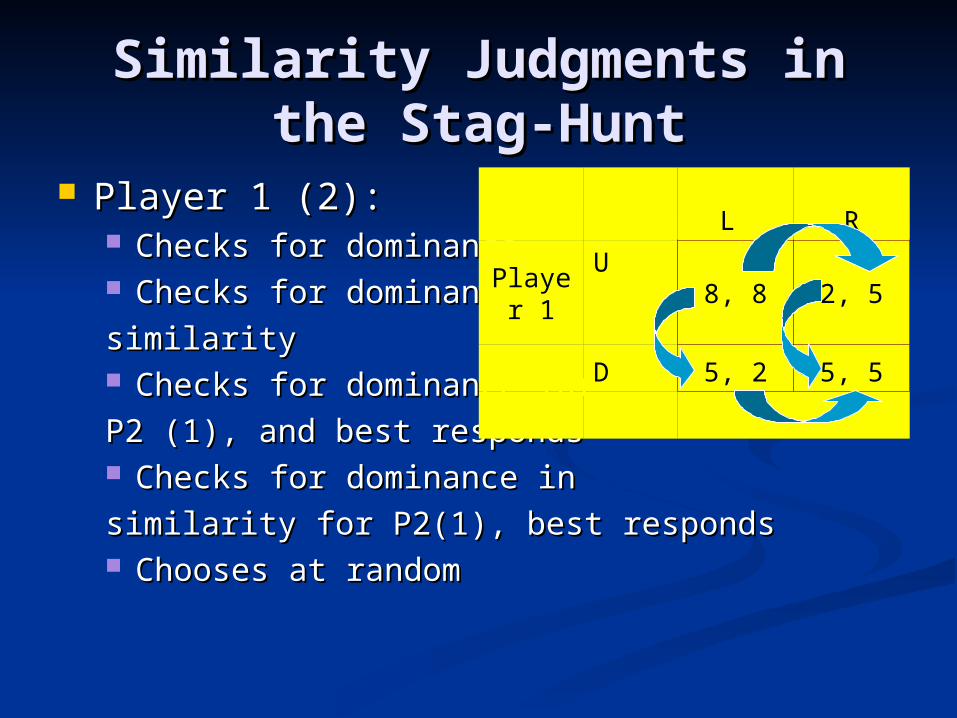
Similarity Judgments in the Similarity Judgments in the Stag-HuntStag-Hunt
Player 1 (2):Player 1 (2): Checks for dominanceChecks for dominance Checks for dominance in Checks for dominance in
similaritysimilarity Checks for dominance for Checks for dominance for
P2 (1), and best respondsP2 (1), and best responds Checks for dominance in Checks for dominance in
similarity for P2(1), best respondssimilarity for P2(1), best responds Chooses at randomChooses at random
L R
Player 1
U 8, 8 2, 5
D 5, 2 5, 5
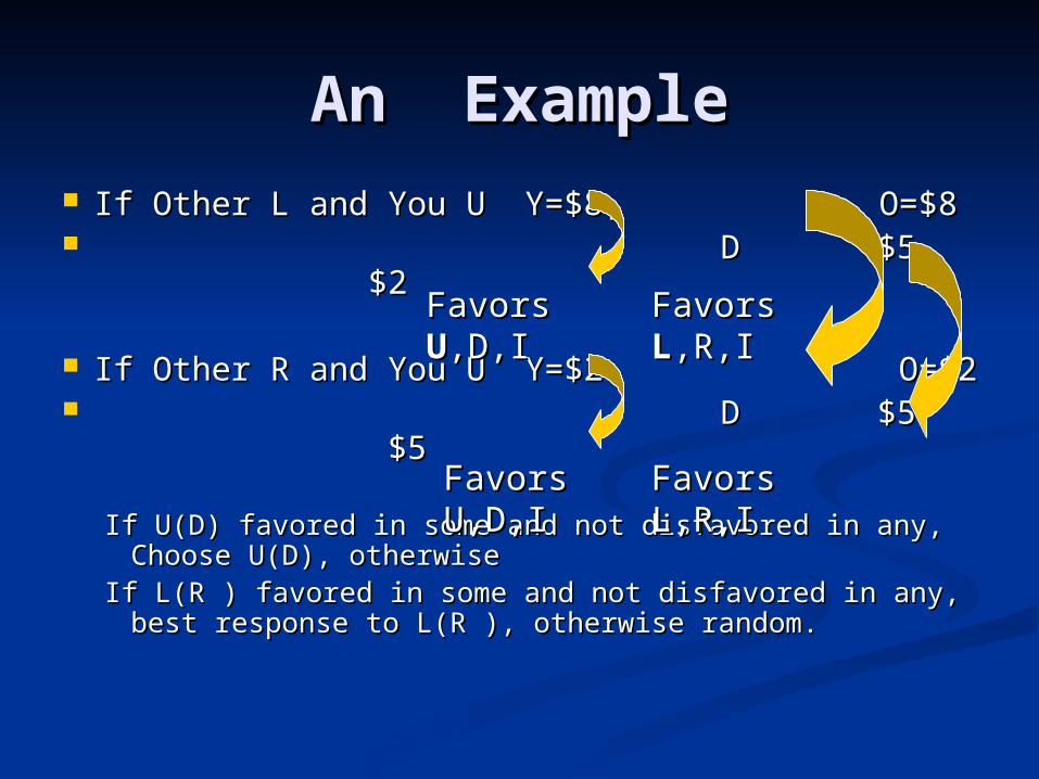
An ExampleAn Example If Other L and You U Y=$8,If Other L and You U Y=$8, O=$8 O=$8 D $5 $2D $5 $2
If Other R and You U Y=$2If Other R and You U Y=$2 O=$2 O=$2 D $5 $5D $5 $5
If U(D) favored in some and not disfavored in any, If U(D) favored in some and not disfavored in any, Choose U(D), otherwiseChoose U(D), otherwise
If L(R ) favored in some and not disfavored in any, If L(R ) favored in some and not disfavored in any, best response to L(R ), otherwise random.best response to L(R ), otherwise random.
Favors Favors UU,D,I,D,I
Favors Favors LL,R,I,R,I
Favors Favors U,D,IU,D,I
Favors L,R,IFavors L,R,I
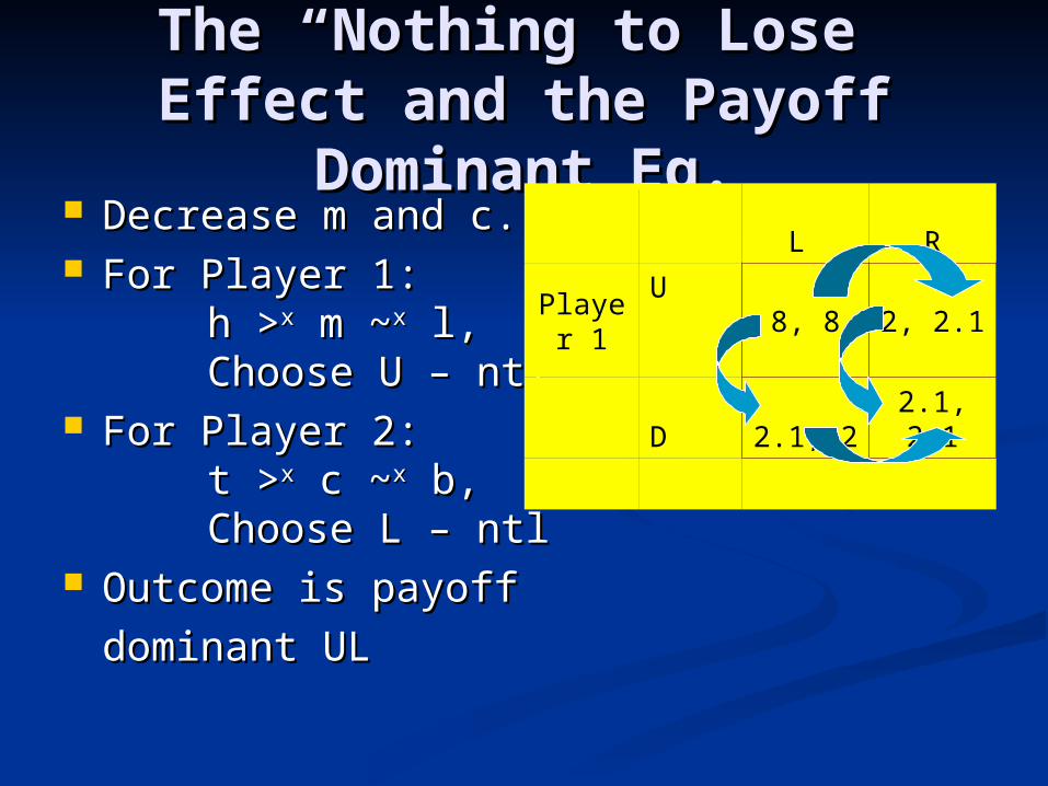
The “Nothing to Lose” The “Nothing to Lose” Effect and the Payoff Effect and the Payoff
Dominant Eq.Dominant Eq. Decrease m and c.Decrease m and c. For Player 1:For Player 1:
h >h >xx m ~ m ~xx l, l,Choose U – ntlChoose U – ntl
For Player 2:For Player 2:t >t >xx c ~ c ~xx b, b,Choose L – ntlChoose L – ntl
Outcome is payoffOutcome is payoff
dominant ULdominant UL
L R
Player 1
U 8, 8 2, 2.1
D 2.1, 2 2.1, 2.1

The “Nothing to Gain” The “Nothing to Gain” Effect and the Security-Effect and the Security-
minded Eq.minded Eq. Increase m and cIncrease m and c For Player 1:For Player 1:
h ~h ~xx m > m >xx l, l,Choose D – ntgChoose D – ntg
For Player 2:For Player 2:t ~t ~xx c > c >xx b, b,Choose R – ntgChoose R – ntg
Outcome is security-Outcome is security-
minded DRminded DR
L R
Player 1
U 8, 8 2, 7.9
D 7.9, 2 7.9, 7.9

The “Nothing to The “Nothing to Gain/Nothing to Lose” Gain/Nothing to Lose”
Effect and Non-eq. Effect and Non-eq. OutcomesOutcomes Increase m, decrease c.Increase m, decrease c.
For Player 1:For Player 1:h ~h ~xx m > m >xx l, l,Choose D – ntgChoose D – ntg
For Player 2:For Player 2:t >t >xx c ~ c ~xx b, b,Choose L – ntlChoose L – ntl
Outcome is non-equilibriumOutcome is non-equilibriumDLDL
L R
Player 1
U 8, 8 2, 2.1
D 7.9, 2 7.9, 2.1
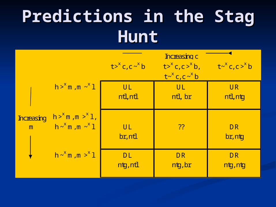
Predictions in the Stag Predictions in the Stag HuntHunt
t >x c, c ~x b t >x c, c >x b,
t ~x c, c ~x b
t ~x c, c >x b
h >x m, m ~x l UL UL URntl, ntl ntl, br ntl, ntg
Increasing m
h >x m, m >x l ,
h ~x m, m ~x l UL ?? DRbr, ntl br, ntg
h ~x m, m >x l DL DR DRntg, ntl ntg, br ntg, ntg
Increasing c

Testing the Ntg/Ntl Effect – Testing the Ntg/Ntl Effect – Experiment DetailsExperiment Details
76 students at the University of Trento 76 students at the University of Trento Experiment consisted of 3 parts, 1Experiment consisted of 3 parts, 1stst of of
which involved games.which involved games. 9 games – 5 stag hunts, 3 matching 9 games – 5 stag hunts, 3 matching
pennies games, 1 additional stag hunt pennies games, 1 additional stag hunt (always last)(always last)
Order otherwise randomizedOrder otherwise randomized Subjects played 1 of games at end of Subjects played 1 of games at end of
session – payouts between 1.20 and 8.00 session – payouts between 1.20 and 8.00 euro.euro.

Games and Individual Games and Individual ResultsResults
L RU 8.00, 8.00 2.00, 2.10 37 (97%)D 2.10, 2.00 2.10, 2.10 1 (3%)
37 (97%) 1 (3%)ntl ntl
L RU 8.00, 8.00 2.00, 5.00 18 (47%)D 5.00, 2.00 5.00, 5.00 20 (53%)
26 (68%) 12 (32%)? ?
L R L R L RU 8.00, 8.00 2.00, 2.10 17 (45%) U 8.00, 8.00 2.00, 5,00 11 (29%) U 8.00, 8.00 2.00, 7.90 14 (37%)D 7.90, 2.00 7.90, 2.10 21 (55%) D 7,90, 2.00 7,90, 5.00 27 (71%) D 7.90, 2.00 7.90, 7.90 24 (63%)
35 (92%) 3 (8%) 20(53%) 18 (47%) 13 (34%) 25 (66%)
Increase
m
Increase c
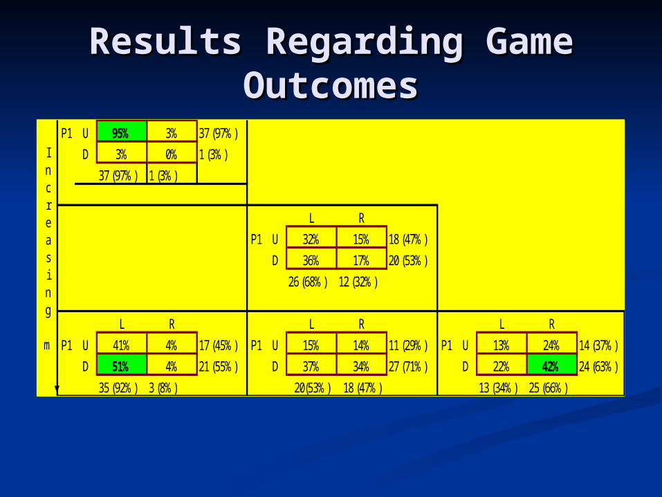
Results Regarding Game Results Regarding Game OutcomesOutcomes
P1 U 95% 3% 37 (97%)
D 3% 0% 1 (3%)
37 (97%) 1 (3%)
L R
P1 U 32% 15% 18 (47%)
D 36% 17% 20 (53%)
26 (68%) 12 (32%)
L R L R L R
P1 U 41% 4% 17 (45%) P1 U 15% 14% 11 (29%) P1 U 13% 24% 14 (37%)
D 51% 4% 21 (55%) D 37% 34% 27 (71%) D 22% 42% 24 (63%)
35 (92%) 3 (8%) 20(53%) 18 (47%) 13 (34%) 25 (66%)
Increasing
m

Performance Relative to Performance Relative to Proposed Selection CriteriaProposed Selection Criteria
Game I-I III-I III-IIIPredominant Eq. Predicted Based on
Player' Responses UL (95%) DL (51%) DR (42%)Equilibrium Selection CriterionMixed Strategies DR 25% each ULPayoff Dominance UL UL ULSecurity-mindedness DR DR DRRisk Dominance UL UL or DR DRntg/ntl UL DL DR

Games of Pure ConflictGames of Pure Conflict
Player’s interestsPlayer’s interests
are diametrically opposedare diametrically opposed No equilibrium in pure No equilibrium in pure
strategies, only a mixedstrategies, only a mixed
strategystrategy
L R
Player 1
U h, b m, t
D l, c h, b
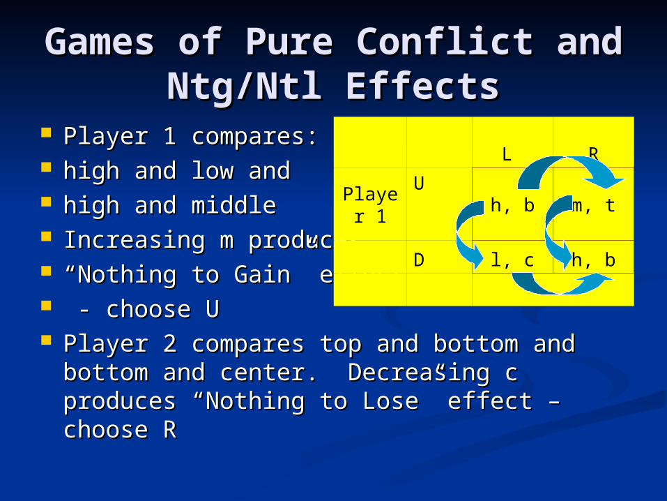
Games of Pure Conflict and Games of Pure Conflict and Ntg/Ntl EffectsNtg/Ntl Effects
Player 1 compares:Player 1 compares: high and low and high and low and high and middlehigh and middle Increasing m producesIncreasing m produces ““Nothing to Gain” effectNothing to Gain” effect - choose U- choose U Player 2 compares top and bottom and Player 2 compares top and bottom and
bottom and center. Decreasing c produces bottom and center. Decreasing c produces “Nothing to Lose” effect – choose R“Nothing to Lose” effect – choose R
L R
Player 1
U h, b m, t
D l, c h, b

Predictions in Conflict Predictions in Conflict GamesGames
t >x b, c ~x b t >x b , c >x b
h >x l,
h >x m DR ??Increasing
mbr, ntl
h >x l,
h ~x m UR URntg, ntl ntg, br
Decreasing c
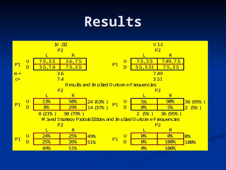
ResultsResults
L R L RU 7.5, 3.5 3.6, 7.5 U 7.5, 3.5 7.49, 7.5D 3.5, 7.4 7.5, 3.5 D 3.5, 3.51 7.5, 3.5
m=c=
L R L RU 13% 50% 24 (63%) U 5% 90% 36 (95%)D 8% 29% 14 (37%) D 0% 5% 2 (5%)
8 (21%) 30 (79%) 2 (5%) 36 (95%)
L R L RU 24% 25% 49% U 0% 0% 0%D 25% 26% 51% D 0% 100% 100%
49% 51% 0% 100%
Results and Implied Outcome Frequencies
IV-III VI-IP2 P2
P1 P1
3.6 7.497.4 3.51
P2 P2
P1 P1
Mixed Strategy Probablilities and Implied Outcome FrequenciesP2 P2
P1 P1
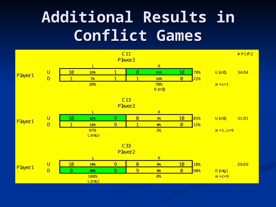
Additional Results in Additional Results in Conflict GamesConflict Games
# P1/P2
U 10 23% 1 0 55% 10 78% U(ntl) 34/34
D 1 7% 1 1 15% 0 22%
m=c=1
U 10 82% 9 0 3% 10 85% U(ntl) 31/31
D 1 15% 9 1 0% 0 15%
m=1, c=9
U 10 10% 9 0 0% 10 10% 29/29
D 9 90% 9 9 0% 0 90% D(ntg)
m=c=9
Player 1
100% 0%L(ntg)
C33Player 2
L R
Player 1
97% 3%L(ntg)
C13Player 2
L R
Player 1
30% 70%R(ntl)
C11Player 2
L R

Across Game ResultsAcross Game Results
1 2L R L R
P1 U 8.00, 8.00 2.00, 2.108.00, 8.00
2.00, 2.10
D 2.10, 2.00 2.10, 2.107.90, 2.00
7.90, 2.10
3 4L R L R
P1 U 8.00, 8.00 2.00, 7.90 7.5, 3.5 7.49, 7.5
D 7.90, 2.00 7.90, 7.90 3.5, 3.51 7.5, 3.5
P1 Predicted Pattern U D D UP2 Predicted Pattern L L R R
Predicted 16 42% 22 58% 38 50%1 Off 11 29% 14 37% 25 33%2 Off 9 24% 1 3% 10 13%3 Off 2 5% 1 3% 3 4%
Player 1 Player 2 Total
P2 P2
P2 P2

Across Game Results cont.Across Game Results cont.
P1 Choice Patterns1 2 3 4 N %
Predicted U D D U 16 42%1 off U U D U 6 16%
U D U U 5 13%2 off U U U U 8 21%
U U D D 1 3%3 off U U U D 1 3%
D U D U 1 3%100%
P2 Choice Patterns1 2 3 4 N %
Predicted L L R R 22 58%1 off L L L R 14 37%2 off L L L L 1 3%3 off R R R L 1 3%
100%
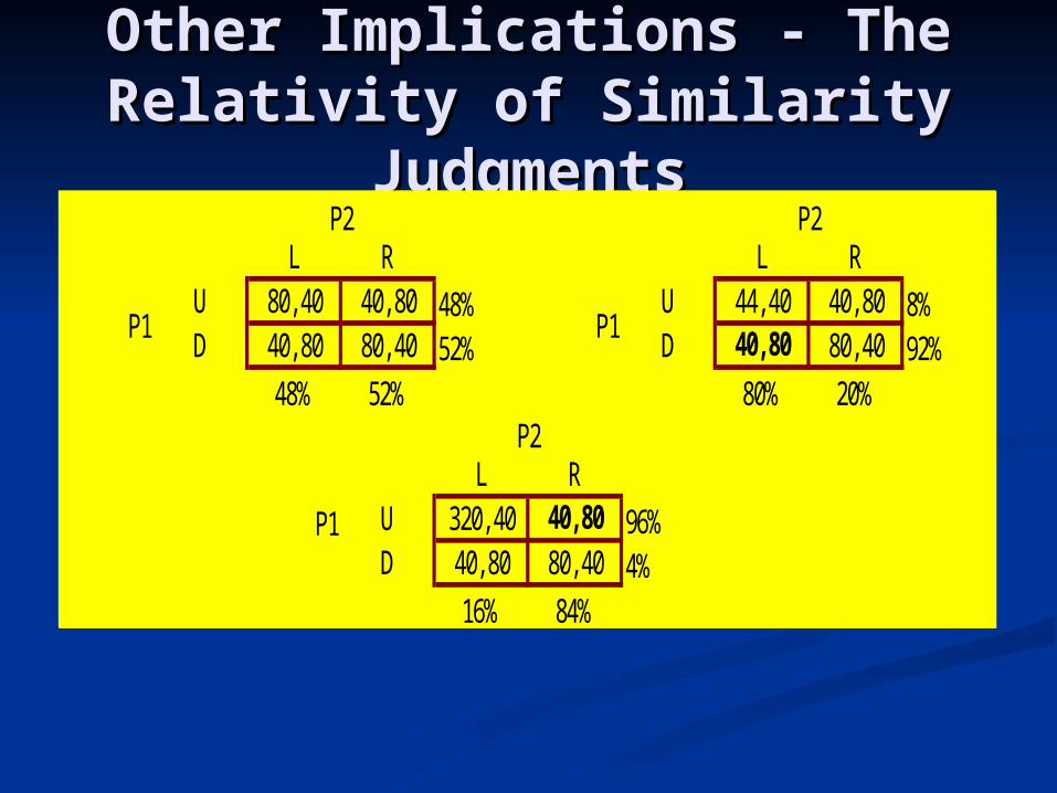
Other Implications - The Other Implications - The Relativity of Similarity Relativity of Similarity
JudgmentsJudgmentsL R L R
U 80, 40 40, 80 48% U 44, 40 40, 80 8%D 40, 80 80, 40 52% D 40, 80 80, 40 92%
48% 52% 80% 20%
L R
P1 U 320, 40 40, 80 96%D 40, 80 80, 40 4%
16% 84%
P2
P1 P1
P2 P2

Similarity Judgments and Similarity Judgments and Framing Effects In Choice Framing Effects In Choice
Under UncertaintyUnder Uncertainty1-20 (20%) 21-40 (20%) 41-80 (40%)81-100 (20%)
A $5 $5 $0 $13B $0 $12 $5 $0
1-20 (20%) 21-40 (20%) 41-80 (40%)81-100 (20%)A' $0 $13 $5 $0B' $5 $5 $0 $12
A' B'A 31 (53%) 18 (31%) 49 (89%)B 5 (8%) 5 (8%) 10 (17%)
36 (61%) 23 (39%

Framing Effects in Games - Framing Effects in Games - Own First vs Other First and non-Own First vs Other First and non-
Equilibrium OutcomesEquilibrium OutcomesL R L R
Player 1 U 8.00, 8.00 2.00, 2.10 Player 1 U 7,20, 7,20 1,20, 1,20D 7.90, 2.00 7.90, 2.10 D 7,10, 1,20 7,10, 1,30
t >x c, c ~x b t >x c, c >x b,
t ~x c, c ~x b
t ~x c, c >x b t >x c, c ~x b t >x c, c >x b,
t ~x c, c ~x b
t ~x c, c >x b
h >x m, m ~x l UL UL UR h >x m, m ~x l UL UL DLntl, ntl ntl, br ntl, ntg br, br ntl, br br, br
Increasing m
h >x m, m >x l ,
h ~x m, m ~x l UL ?? DRIncreasing
m
h >x m, m >x l ,
h ~x m, m ~x l UL ?? DRbr, ntl br, ntg br, ntl br, ntg
h ~x m, m >x l DL DR DR h ~x m, m >x l UR DR DRntg, ntl ntg, br ntg, ntg br, br ntg, br br, br
Increasing c Increasing c
III-I III-I*Player 2 Player 2
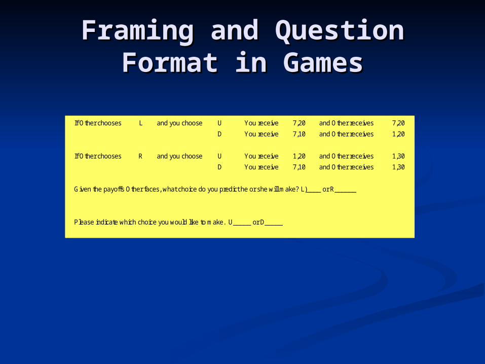
Framing and Question Framing and Question Format in GamesFormat in Games
If Other chooses L and you choose U You receive 7,20 and Other receives 7,20
D You receive 7,10 and Other receives 1,20
If Other chooses R and you choose U You receive 1,20 and Other receives 1,30
D You receive 7,10 and Other receives 1,30
Given the payoffs Other faces, what choice do you predict he or she will make? L)____ or R______
Please indicate which choice you would like to make. U_____ or D_____
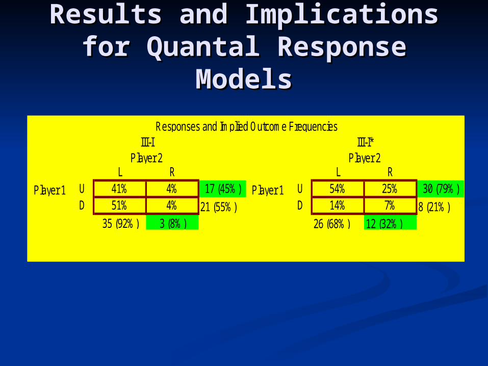
Results and Implications Results and Implications for Quantal Response for Quantal Response
ModelsModels
L R L R
Player 1 U 41% 4% 17 (45%) Player 1 U 54% 25% 30 (79%)D 51% 4% 21 (55%) D 14% 7% 8 (21%)
35 (92%) 3 (8%) 26 (68%) 12 (32%)
Responses and Implied Outcome FrequenciesIII-I III-I*
Player 2 Player 2

What Would You Choose?What Would You Choose?
For Player 1W U You receive 6 and Other receives 13
D 12 12
X U You receive 5 and Other receives 5D 8 8
Y U You receive 2 and Other receives 7D 6 6
Z U You receive 13 and Other receives 2D 2 2
If other chooses and you choose
If other chooses and you choose
If other chooses and you choose
If other chooses and you choose

Level-1 Bounded Level-1 Bounded Rationality vs. SimilarityRationality vs. Similarity
U 2 13 13 5 5 7 7 2 6.75
D 12 12 8 8 6 6 2 2 7
12.5 6.5 6.5 2
U 13 13 5 5 7 7 2 2 6.75
D 2 12 12 8 8 6 6 2 7
12.5 6.5 6.5 2
U 7 13 5 5 2 7 13 2 6.75
D 12 12 8 8 6 6 2 2 7
12.5 6.5 6.5 2
Z
Player 1
Player 2W X Y Z
W X
Player 1
Y
Y Z
Player 1
EQ and Similarity and Level-1 predict DW
Similarity and EQ predicts U, Level-1 predicts D
EQ and L1 predict D, Similarity allows U
Player 2W X
Player 2
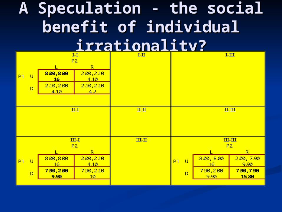
A Speculation - the social A Speculation - the social benefit of individual benefit of individual
irrationality?irrationality?L R
P1 U8.00, 8.00
162.00, 2.10
4.10
D2.10, 2.00
4.102.10, 2.10
4.2
L R L R
P1 U8.00, 8.00
162.00, 2.10
4.10P1 U
8.00, 8.00 16
2.00, 7.90 9.90
D7.90, 2.00
9.907.90, 2.10
10D
7.90, 2.00 9.90
7.90, 7.90 15.80
III-I III-IIIP2 P2
III-II
II-I II-IIIII-II
I-I I-IIIP2
I-II

A Speculation - the social A Speculation - the social benefit of individual benefit of individual irrationality? (cont.)irrationality? (cont.)
U 10 11 1 0 10 10D 1 2 1 1 1 0
U 10 19 9 0 10 10D 1 10 9 1 1 0
U 10 19 9 0 10 10D 9 18 9 9 9 0
Player 1
Player 2L R
Player 1
C13Player 2
L R
Player 1
C33Player 2
L R

A Speculation - the social A Speculation - the social benefit of non-strategic benefit of non-strategic thinking and limits to thinking and limits to
learninglearning
L R L RU 8.00, 8.00 2.00, 2.10 U 7.20, 7,20 1.20, 1.20D 7.90, 2.00 7.90, 2.10 D 7.10, 1.20 7.10, 1.30
Player 1
Player 1
III-I III-I*Player 2 Player 2
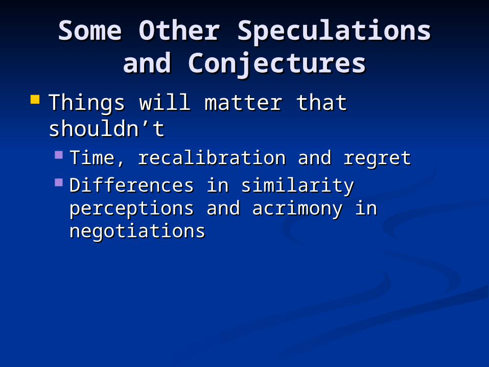
Some Other Speculations Some Other Speculations and Conjecturesand Conjectures
Things will matter that shouldn’tThings will matter that shouldn’t Time, recalibration and regretTime, recalibration and regret Differences in similarity perceptions Differences in similarity perceptions
and acrimony in negotiationsand acrimony in negotiations

ConclusionsConclusions
Many choice anomalies can be explained if Many choice anomalies can be explained if people employ “nothing to gain/nothing to people employ “nothing to gain/nothing to lose reasoning”lose reasoning”
The same reasoning process applied to The same reasoning process applied to games predicts:games predicts: play in coordination and conflict games and play in coordination and conflict games and
the successes and failures of equilibrium selection the successes and failures of equilibrium selection criteria and mixed strategy choicecriteria and mixed strategy choice
systematic differences in play as a consequence systematic differences in play as a consequence of theoretically inconsequential changes in the of theoretically inconsequential changes in the way strategy choices are elicited.way strategy choices are elicited.

ReferencesReferences Camerer, C. Behavioral Game Theory: Experiments on Strategic Interaction, Camerer, C. Behavioral Game Theory: Experiments on Strategic Interaction, Princeton, 2003.Princeton, 2003. Camerer, C., Teck-Hua Ho and Juin Kuan Chong. Camerer, C., Teck-Hua Ho and Juin Kuan Chong.
Behavioral Game Theory: Thinking, Learning and Teaching,"Behavioral Game Theory: Thinking, Learning and Teaching," with Teck-Hua Ho and Juin Kuan with Teck-Hua Ho and Juin Kuan Chong. Forthcoming in a book edited by Steffen Huck, Chong. Forthcoming in a book edited by Steffen Huck, Essays in Honor of Werner Guth."Essays in Honor of Werner Guth."
Goerree, J. and C. Holt. “Ten Little Treasures of Game Theory and Ten Intuitive Goerree, J. and C. Holt. “Ten Little Treasures of Game Theory and Ten Intuitive Contradictions.” American Economic Review. 2001. Vl. 91(5), pp 1402-1422.Contradictions.” American Economic Review. 2001. Vl. 91(5), pp 1402-1422. Haruvy, E. and D. Stahl. “Deductive versus Inductive equilibrium selection” Haruvy, E. and D. Stahl. “Deductive versus Inductive equilibrium selection” experimental results.” Journal of Economic Behavior and Organization. 2004, 53, 319-331.experimental results.” Journal of Economic Behavior and Organization. 2004, 53, 319-331. Keser, C. and B. Vogt. “Why do experimental subjects choose an equilibrium which Keser, C. and B. Vogt. “Why do experimental subjects choose an equilibrium which is neither risk nor payoff dominant?” Cirano Working Paper. 2000. is neither risk nor payoff dominant?” Cirano Working Paper. 2000.
http://www.cirano.qc.ca/pdf/publication/2000s-34.pdfhttp://www.cirano.qc.ca/pdf/publication/2000s-34.pdf Leland, J. "Generalized Similarity Judgments: An Alternative Explanation for Choice Anomalies." Leland, J. "Generalized Similarity Judgments: An Alternative Explanation for Choice Anomalies."
Journal of Risk and UncertaintyJournal of Risk and Uncertainty, 9, 1994, 151-172. , 9, 1994, 151-172. Leland, J. “Similarity Judgments in Choice Under Uncertainty: A Reinterpretation of Regret Leland, J. “Similarity Judgments in Choice Under Uncertainty: A Reinterpretation of Regret
Theory.” Theory.” Management ScienceManagement Science, 44(5), 1998, 1-14., 44(5), 1998, 1-14. Leland, J. “Similarity Judgments and Anomalies in Intertemporal Choice.” Leland, J. “Similarity Judgments and Anomalies in Intertemporal Choice.” Economic Inquiry Economic Inquiry Vol. Vol.
40, No. 4, October 2002, 574-581. 40, No. 4, October 2002, 574-581. Lowenstein, G. and D. Prelec. "Anomalies in Intertemporal Choice: Evidence and Interpretation." Lowenstein, G. and D. Prelec. "Anomalies in Intertemporal Choice: Evidence and Interpretation."
The Quarterly Journal of EconomicsThe Quarterly Journal of Economics, May 1992, 573-597., May 1992, 573-597. Rubinstein, A. "Similarity and Decision-making Under Risk (Is There a Utility Theory Resolution to Rubinstein, A. "Similarity and Decision-making Under Risk (Is There a Utility Theory Resolution to
the Allais Paradox?)." the Allais Paradox?)." Journal of Economic TheoryJournal of Economic Theory, 46, 1988, 145-153., 46, 1988, 145-153. Rubinstein, A. “Economics and Psychology"? The Case of Hyperbolic Discounting, Rubinstein, A. “Economics and Psychology"? The Case of Hyperbolic Discounting, International International
Economic ReviewEconomic Review 44, 2003, 1207-1216. 44, 2003, 1207-1216. Standord Encycolpedia of Philosophy. http://plato.stanford.edu/entries/game-theory/Standord Encycolpedia of Philosophy. http://plato.stanford.edu/entries/game-theory/

Testing the Ntg/Ntl Effect – Testing the Ntg/Ntl Effect – Question FormatQuestion Format
If Other chooses L and you choose U You receive 8,00 and Other receives 8,00D You receive 5,00 and Other receives 2,00
If Other chooses R and you choose U You receive 2,00 and Other receives 5,00D You receive 5,00 and Other receives 5,00
The ProblemThe Problem
““existing deductive selection rules have been shown to do poorly in experiments” (Haruvy & Stahl, 2004), 2004)
Should we be surprised?Should we be surprised? “…Game theory is the study strategic
interactions among rational players..”” We know people behave irrationally in
risky and intertemporal choice situations – why would we expect them to do better in complex strategic settings?

A Speculation - A Speculation - the problem with being the problem with being
strategic in a non-strategic strategic in a non-strategic worldworld
L R L R
Player 1 U 8.00, 8.00 2.00, 2.10 Player 1 U 7,20, 7,20 1,20, 1,20D 7.90, 2.00 7.90, 2.10 D 7,10, 1,20 7,10, 1,30
t >x c, c ~x b t >x c, c >x b,
t ~x c, c ~x b
t ~x c, c >x b t >x c, c ~x b t >x c, c >x b,
t ~x c, c ~x b
t ~x c, c >x b
h >x m, m ~x l UL UL UR h >x m, m ~x l UL UL DLntl, ntl ntl, br ntl, ntg br, br ntl, br br, br
Increasing m
h >x m, m >x l ,
h ~x m, m ~x l UL ?? DRIncreasing
m
h >x m, m >x l ,
h ~x m, m ~x l UL ?? DRbr, ntl br, ntg br, ntl br, ntg
h ~x m, m >x l DL DR DR h ~x m, m >x l UR DR DRntg, ntl ntg, br ntg, ntg br, br ntg, br br, br
Increasing c Increasing c
III-I III-I*Player 2 Player 2