Non-destructuve tests in roads and airfields A study of ...

Non-destructive tests in roads and airfields

A study of the Falling Weight Deflectometer

Edgar Alexandre Chong Cardoso

Thesis to obtain the Master of Science Degree in

Civil Engineering

Supervisor: Prof. José Manuel Coelho das Neves

Examination Committee

Chairperson:

Supervisor:

Members of the Committee:

Prof. João Torres de Quinhones Levy

Prof. José Manuel Coelho das Neves

Prof. Luís Guilherme de Picado Santos

November 2017

i

Acknowledgement

The present dissertation was developed with close guidance and supervision of Professor Doctor José Neves whom I wish to extend my immense gratitude towards his dedication in the completion of this project. Without his belief and enthusiasm this work would not have been possible. It is my great pleasure to thank those who made this thesis possible, the institutions involved in the experimental research included in this work.: Instituto Superior Técnico (Professor Doctor Luís Picado Santos and César Abreu), Laboratório Nacional de Engenharia Civil (Vitor Antunes, Vânia Marecos), Força Aérea Portuguesa – Laboratório Solos e Pavimentos (Lieutenant Henrique Rodrigues and the officers involved). The proficiency test was organized under coordination of RELACRE, with Cláudia Silva and Ana Maria Duarte, whom kindly released all data necessary in developing this project.

To my Parents that endured so much and did not stop motivating me through hardship for so long.

To my grandfather Ming Lam whom I miss dearly and wished he could witness my achievements.

To my cousin Noel for the long hours of motivation talk and guidance.

To all my friends that provided the utmost support and belief at all times. My special thanks to Paulo Chainho and Ana Rita Martins, who contributed to the completion of the project.

To the medical staff that have given me a second chance to live fully.

Lastly, I would like to send my best regards to all those who were directly or indirectly involved in any respect during the completion of this dissertation.

iii

Resumo

O património rodoviário é um ativo de elevada importância no desenvolvimento das sociedades modernas e a sua qualidade geral desempenha um papel fundamental na segurança, economia, competitividade e sustentabilidade da circulação de pessoas e bens. A degradação dessa qualidade ao longo do tempo deve ser avaliada de forma a que as ações de conservação e reabilitação possam ser adequadamente planeadas para assegurar os padrões mínimos de qualidade especificados. No âmbito do estado dos pavimentos, são vários os indicadores estabelecidos na avaliação da qualidade. Em termos da avaliação estrutural, o defletómetro de impacto – Falling Weight Deflectometer (FWD) – é o ensaio não destrutivo mais utilizado na avaliação da capacidade de carga de pavimentos rodoviários e aeroportuários. Os resultados deste ensaio são da maior importância em vários contextos, como por exemplo na auscultação estrutural dos pavimentos existentes em obras de reabilitação de infraestruturas rodoviárias ou aeroportuárias.

A presente dissertação tem como objetivos principais a avaliação da precisão e da incerteza das deflexões medidas no ensaio com o FWD e a análise da sua influência na qualidade de interpretação desses mesmos ensaios, ou seja, das características de deformabilidade dos pavimentos existentes obtidas por retroanálise, com vista à avaliação da sua qualidade estrutural e apoio ao projeto de reabilitação.

A metodologia adotada baseou-se na realização de um ensaio de aptidão segundo a norma ISO/IEC 17043 com a participação de três equipamentos de fabricantes diferentes e pertencentes a entidades nacionais. Os resultados obtidos foram analisados quanto à repetibilidade e reprodutibilidade e, posteriormente, procedeu-se à quantificação da incerteza. Atendendo aos resultados obtidos nesta análise, procedeu-se a um estudo de sensibilidade da influência da incerteza das deflexões medidas nos módulos de deformabilidade das camadas do pavimento e fundação, obtidos da interpretação dos resultados dos ensaios (retroanálise) para o caso de pavimentos flexíveis.

Em geral, os resultados confirmaram uma boa repetibilidade das deflexões, contrastando com níveis por vezes muito baixos de reprodutibilidade. Por consequência, a incerteza revelou-se grande. Constatou-se ainda que a precisão e a incerteza dependeram do tipo de pavimento e da magnitude das deflexões. A incerteza foi maior em pavimentos flexíveis e para deflexões também maiores. Em relação à análise de sensibilidade da influência da incerteza na interpretação dos resultados do FWD, verificou-se que a sensibilidade à incerteza é maior em pavimentos mais flexíveis, nomeadamente em relação à análise da deformabilidade dos materiais da fundação.

Palavras-chave: defletometro de impacto, pavimentos, repetibilidade, reprodutibilidade,

incerteza, retroanálise

v

Abstract

Road infrastructure is a high value asset in the development of modern society where its perceived quality translates into a fundamental role in security, economy, competitivity and sustainability of the free flow of people and goods. The gradual degradation of that quality through time should be evaluated in such a manner that maintenance and rehabilitation efforts can be timely planned and carried out to maintain its specified minimum quality requirements. In pavement condition assessment, there are several parameters that gauge pavement quality. The Falling Weight Deflectometer (FWD), is the main non-destructive testing equipment used to assess the bearing capacity of road and airfield pavements. This test’s results are very relevant in several contexts, for example, a survey for bearing capacity in existing road or airfield pavements requiring rehabilitation intervention.

The present dissertation’s objective is to assess the precision and uncertainty performance in measuring deflection and to analyze its influence in the quality of results from the testing campaign, therefore assessing the structural capacity of existing pavements (backanalysis), in view to evaluate the structural quality and support a rehabilitation project.

The adopted methodology consisted in a proficiency test scheme (PTS) field test compliant with ISO/IEC 17043 featuring a fleet of three FWD from different manufactures and owned by portuguese operators. The obtained deflection data was firstly processed for repeatability and reproducibility, and afterwards analyzed for uncertainty quantification. Lastly, the resulting data was used for a sensitivity analysis featuring the uncertainty of the measured deflection influence on the mechanical properties (elastic moduli) estimated from the field survey (backanalysis) on flexible pavements.

The experimental research results confirmed a satisfactory repeatability of deflection measurements. In contrast, the reproducibility is difficult to achieve in most cases. Consequently, the uncertainty levels revealed to be high. Uncertainty and precision revealed to be dependent of pavement type and deflection magnitude. Uncertainty presented high values for flexible pavement and for high deflections. Regarding to the sensitivity analysis on the uncertainty’s influence on the FWD results interpretation, it was concluded that the flexible pavements presented higher sensibility to uncertainty mainly when gauging for stiffness on the foundation layers.

Keywords: falling weight deflectometer, pavements, repeatability, reproducibility, uncertainty,

backcalculation

vii

Table of contents

Acknowledgement .......................................................................................................................... i

Resumo ......................................................................................................................................... iii

Abstract ......................................................................................................................................... v

Table of contents .......................................................................................................................... vii

List of figures ................................................................................................................................. xi

List of tables ................................................................................................................................ xiii

Abbreviations ................................................................................................................................ xv

1 Introduction............................................................................................................................. 1

1.1 Background and aim...................................................................................................... 1

1.2 Objectives ...................................................................................................................... 1

1.3 Methodology .................................................................................................................. 2

1.4 Dissertation structure..................................................................................................... 2

2 Literature review ..................................................................................................................... 5

2.1 Nondestructive pavement tests ..................................................................................... 5

2.1.1 Introduction ................................................................................................................ 5

2.1.2 Road surface condition .............................................................................................. 6

2.1.3 Bearing capacity assessment .................................................................................... 7

2.2 Falling Weight Deflectometer ........................................................................................ 9

2.2.1 Introduction ................................................................................................................ 9

2.2.2 Operation principle .................................................................................................. 11

2.2.3 Load force ................................................................................................................ 12

2.2.4 Dampening system .................................................................................................. 12

2.2.5 Load pulse ............................................................................................................... 13

2.2.6 Geophones .............................................................................................................. 14

2.3 Backcalculation ............................................................................................................ 15

2.3.1 Introduction .............................................................................................................. 15

2.3.2 Principles and complexity ........................................................................................ 16

2.3.3 Classical backcalculation methods .......................................................................... 20

viii

2.3.4 Modern optimization techniques .............................................................................. 20

2.4 FWD Accuracy ............................................................................................................. 21

2.5 Summary ..................................................................................................................... 22

3 Proficiency Test .................................................................................................................... 25

3.1 Introduction .................................................................................................................. 25

3.2 Equipment ................................................................................................................... 25

3.3 Test facility ................................................................................................................... 27

3.4 Testing procedure........................................................................................................ 28

3.5 Results ......................................................................................................................... 29

3.6 Summary ..................................................................................................................... 31

4 Data analysis ........................................................................................................................ 33

4.1 Repeatability and reproducibility ................................................................................. 33

4.2 Uncertainty assessment .............................................................................................. 35

4.3 Sensitivity analysis ...................................................................................................... 36

4.4 Test site backcalculation ............................................................................................. 44

4.5 Summary ..................................................................................................................... 46

5 Conclusion and recommendations ....................................................................................... 49

5.1 Summary ..................................................................................................................... 49

5.2 Conclusions ................................................................................................................. 49

5.3 Recommendations....................................................................................................... 51

References .................................................................................................................................. 53

Appendix ...................................................................................................................................... 59

Appendix I. Proficiency test protocol ...................................................................................... 61

Appendix I. FWD results ......................................................................................................... 63

Appendix II. Smoothing filter test ............................................................................................. 65

Appendix III. Repeatability and Reproducibility, N=3 ........................................................... 67

Appendix IV. Repeatability and Reproducibility, N=2 ........................................................... 69

Appendix V. Critical values ...................................................................................................... 71

Appendix VI. Pavement structures ........................................................................................ 73

ix

Appendix VII. Backcalculation of pavement structures .......................................................... 75

Appendix VIII. Test site 1 backcalculation .............................................................................. 81

xi

List of figures

Figure 2.1 - Benkelman Beam in use AASHO Road Test, ca 1962 (Alvin Benkelman Jr.) .......... 5

Figure 2.2 – Traffic Speed Deflectometer (ARRB Group Inc. USA) ............................................. 8

Figure 2.3 – Falling Weight Deflectometer .................................................................................... 9

Figure 2.4 – Heavy Weight Deflectometer .................................................................................. 10

Figure 2.5 – The first Danish Falling Weight (Bohn, 1989) ......................................................... 10

Figure 2.6 - FWD detailed overview ............................................................................................ 11

Figure 2.7 – Realistic FWD loading model (Madsen & Levenberg, 2017) .................................. 12

Figure 2.8 - Pulse time definition (FAA/SRA International, 2014) ............................................... 13

Figure 2.9 – Measured (dotted) and modeled (solid line) FWD load-time histories (Madsen & Levenberg, 2017) ........................................................................................................................ 14

Figure 2.10 - Deflection basin ..................................................................................................... 15

Figure 2.11 - Evaluation of the effect of frequency and of temperature to the proposed correction model (Flores et al., 2017) .......................................................................................................... 19

Figure 2.12 - Effect of smoothing on deflections of FWD (Van Gurp, 1995) .............................. 19

Figure 2.13 - Fourier transform of two half-sine shock pulses (Van Gurp, 1995) ....................... 20

Figure 3.1 - FWD equipment ....................................................................................................... 26

Figure 3.2 – Test site 1 ................................................................................................................ 27

Figure 3.3 - Deflection charts and Load Pulse influence in deflection measurements ............... 30

Figure 4.1 - Repeatability limits for deflection measurements .................................................... 34

Figure 4.2 - Reproducibility limits for deflection measurements ................................................. 34

Figure 4.3 - Uncertainty of deflection measurements ................................................................. 35

Figure 4.4 - Flexible pavements from MACOPAV manual, F3 foundation ................................. 37

Figure 4.5 –Flexible pavements from MACOPAV manual, F2 foundation .................................. 37

Figure 4.6 – Deflection charts with backcalculated curves (F3 subgrade class, 65 kN) ............. 38




Figure 4.10 – Variation in critical stiffness values in relation to percentage of asphalt concrete layer thickness over pavement’s total thickness ......................................................................... 43

Figure 4.11 – Deflection chart with BC curve, Site 1, 65 kN ....................................................... 44

xii

Figure 4.12 – Deflection chart with BC curve, Site 1, 90 kN ....................................................... 45

Figure. VIII.1 - Backcalculated deflections (65 kN and 90 kN) .................................................... 82

xiii

List of tables

Table 2.1 – Categories of deflection measurement equipment .................................................... 7

Table 2.2 - Common elastic moduli values (Estradas de Portugal, 1995) .................................. 16

Table 2.3 – Stiffness modulus for the asphalt layer (Pais & Pereira, 2017) ............................... 18

Table 3.1 - Main specifications of FWD equipment ..................................................................... 26

Table 3.2 – Characteristics of the test sites ................................................................................ 27

Table 3.3 – Test protocol ............................................................................................................. 28

Table 3.4 - Sequence of events .................................................................................................. 28

Table 4.1 - Repeatability and reproducibility limits ...................................................................... 34

Table 4.2 – Interval of pavement layer moduli, F3 subgrade class, 65 kN and 90 kN ................ 42

Table 4.3 – Interval of pavement layer moduli, F3 subgrade class, 65 kN and 90 kN ................ 42

Table 4.4 – Backcalculation results for Site 1, 65 kN .................................................................. 46

Table 4.5 – Backcalculation results for Site 1, 90 kN .................................................................. 46

Table. I.1 - Site 1, 65 kN .............................................................................................................. 63

Table. I.2 - Site 1, 90 kN .............................................................................................................. 63

Table. I.3 - Site 2, 90 kN .............................................................................................................. 64

Table. II.1 – Smoothing filter test results, Test site 1 .................................................................. 65

Table. II.2 - Smoothing filter test results, LNEC rigid pavement ................................................. 65

Table. III.1 – Cochran’s test ........................................................................................................ 67

Table. III.2 - Grubb’s test ............................................................................................................. 67

Table. III.3 - Site 1, 65 kN ............................................................................................................ 67

Table. III.4 - Site 1, 90 kN ............................................................................................................ 68

Table. III.5 - Site 2, 90 kN ............................................................................................................ 68

Table. IV.1 – Cochran’s test ........................................................................................................ 69

Table. IV.2 - Grubb’s test ............................................................................................................ 69

Table. IV.3 - Site 1, 65 kN ........................................................................................................... 69

Table. IV.4 - Site 1, 90 kN ........................................................................................................... 70

Table. IV.5 - Site 2, 90 kN ........................................................................................................... 70

Table. V.1 – Critical values, Site 1, 65 kN ................................................................................... 71

xiv

Table. V.2 – Critical values. Site 1, 90 kN ................................................................................... 71

Table. V.3 – Critical values, Site 2, 90 kN ................................................................................... 72

Table. VI.1 – Reference layer moduli .......................................................................................... 73

Table. VII.1 - F3, asphalt bound base 0.12, 65 kN...................................................................... 75


Table. VII.3 - F3, unbound granular base 0.10, 65 kN ................................................................ 75

Table. VII.4 - F3, unbound granular base 0.26 ........................................................................... 75



Table. VII.7 - F2, unbound granular base 0.12, 65 kN ................................................................ 76

Table. VII.8 - F2, unbound granular base 0.28, 65 kN ...................................................................... 76


Table. VII.10 - F3, asphalt bound base 0.28, 90 kN.................................................................... 77

Table. VII.11 - F3, unbound granular base 0.10, 90 kN .............................................................. 77

Table. VII.12 - F3, unbound granular base 0.26, 90 kN .............................................................. 77

Table. VII.13– F2, asphalt bound base 0.16, 90 kN .................................................................... 78

Table. VII.14 – F2, asphalt bound base 0.32, 90 kN ................................................................... 78

Table. VII.15 – F2, unbound granular base 0.12, 90 kN ............................................................. 78

Table. VII.16 – F2, unbound granular base 0.28, 90 kN ............................................................. 78

Table. VII.17 - Sensitivity analysis, Percentage of top layer over pavement total thickness ...... 79

Table. VIII.1 – Test site 1 backcalculation ................................................................................... 81

xv

Abbreviations

AASHO American Association of States Highways Officials

AASHTO American Association of State Highway and Transportation Officials

ASTM American Society for Testing and Materials

BC Backcalculation

EuroFWD European Falling Weight Deflectometer User Group

FWD Falling Weight Deflectometer

FWDUG Falling Weight Deflectometer User Group

GPR Ground Penetrating Radar

HWD Heavy Weight Deflectometer

IST Instituto Superior Técnico

LDVT Linear Differential Vertical Transducers

LNEC Laboratório Nacional de Engenharia Civil

LSP Laboratório de Solos e Pavimentos – Força Aérea Portuguesa

LTPP Long-Term Pavement Performance

LWD Light Weight Deflectometer

M&R Maintenance and rehabilitation

MACOPAV Manual de Concepção de Pavimentos para a Rede Rodoviária Nacional

MEPDG Mechanistic-Empirical Pavement Design Guide

NCAT National Center for Asphalt Institute

NCHRP National Cooperative Highway Research Program

NDT Non-Destructive Test

PMS Pavement Management System

PTS Proficiency Test Scheme

RDT Road Deflection Tester

RELACRE Associação de Laboratórios Acreditados de Portugal

RMSE Root Mean Square Error

SF Smoothing Filter

TSD Traffic Speed Deflectometer

1

1 Introduction

1.1 Background and aim

Looking at the European Union statistic data, the Trans-European networks in transport (TEN-T) plays a vital role to promote people and goods circulations between member states (Eurostat, 2014). By promoting business and easy people circulation, transportation strategies are an effective way to tackle inclusion of state members and its citizens. Eurostat data referring to modal split of transportation in EU (Eurostat, 2017) shows that road transport is still by far the most common, representing about 75% of total tonne-kilometers of freight transported. Data forecasts expect a continuing rise of freight transport by road in the foreseeable future. Consequently, new and existing infrastructure assets can benefit from planned maintenance to prolong its life span and reduce the involved financial costs. In a report commended by the European Commission (Steer Davies Gleave, 2009), EU countries invested in total €859 billion in its transport infrastructure sector between 2000 and 2006. A significant portion of the budget was used towards road maintenance to keep existing infrastructures at an acceptable level of service. This sector has proven its significance given the large sum invested thus incentivizing pavement engineering to continually improve (COST, 1997).

Maintenance and rehabilitation (M&R) requires both minimizing administration and user costs while still maintaining infrastructures at high level of service (Meneses & Ferreira, 2012). To manage pavements at network level, administration rely on pavement management systems (PMS) which aggregate road condition data by road sections. This information is in turn analyzed to clearly prioritize interventions to the most critical road sections (Fwa, et al, 2000). Road and airfield administrations are the main clients for the services provided by pavement condition assessment companies. These survey proceedings are regulated by international standards (ASTM, 2008, 2009) using equipment capable of measuring and recording pavement parameters to assessment its condition. One of the most used equipment today is the Falling Weight Deflectometer (FWD), a stationary impulse load deflectometer which will be studied in depth in the following sections of present dissertation.

Although equipment manufacturers guarantee high reliability and repeatability levels through periodic calibration, generally, equivalent models from different manufacturers are less likely to reproduce each other’s measurements. Several authors research (Garg, 2002; Murphy, 1998; Rocha et al, 2004) mention the repeatability and reproducibility issues associated with the FWD which should be taken in consideration and carefully assessed in practice. To empower administration decision makers with informed decisions while executing pavement surveys, it is necessary to experimentally analyze the actual reliability level of existing FWD fleets in current available service providers and thus clearly quantifying existing differences.

This dissertation aims to investigate the precision performance of a FWD fleet under a controlled environment, and mainly to quantify the level of uncertainty in deflection measurements which ultimately influence the quality of the backcalculation process. It is crucial for the administration to have a good understanding of the uncertainty involved in this process which may lead to rehabilitation project designs that may prove to be ineffective and financially inefficient.

1.2 Objectives

The present dissertation objectives are:

2

i. Assess FWD uncertainty and precision performance in measuring deflection with actual collection of test data;

ii. Assess uncertainty’s influence on the quality of backcalculated elastic moduli by perform a sensitivity analysis.

1.3 Methodology

The dissertation presents a thorough literature review about non-destructive pavement testing and the available analytic methods. The first part of the dissertation focuses on reviewing relevant journals and papers currently available on pavement engineering on both network level and project level. This approach provides the necessary framework for the subjects studied in this work. After a brief introduction to NDT, the FWD is fully described, with special emphasis to the components that are reported to be the main sources of FWD uncertainty.

A field test is organized to gather several FWD equipment from various operators. To provide the necessary experimental data, a proficiency test scheme compliant with norm ISO/IEC 17043 (ISO, 2010) was devised to measure pavement deflections in a predetermined test site. From the experimental data, repeatability and reproducibility analysis compliant with ISO 5725-2 is performed. The results are used to frame the experiment for an uncertainty assessment which studies intervals of maximum and minimum values of deflections produced for any given measurement.

Finally, through a set of previously chosen standardized theoretical pavements models (JAE, 1995), a linear elastic layer model computer software BISAR (Shell, 1995) was used to perform backcalculations to assess the respective pavement stiffness. A sensitivity analysis on the resulting elastic moduli is performed to study the influence of the FWD uncertainty on the quality of backcalculation. As a final case study, Test site 1 is backcalculated and the results analyzed.

1.4 Dissertation structure

This dissertation is subdivided in a total of five chapters:

Chapter 1, is the introductory section where the chosen subject is framed. The

dissertation’s aim, objectives, adopted methodology and the dissertation structure is

announced as the guideline for this project.

Chapter 2 follows with a thorough literature review on various key subjects such a brief

introduction on non-destructive road tests, and specifically, the bearing capacity test

equipment FWD. An in-depth FWD study is performed mainly focusing in detail its

functional components that are identified as sources of errors, uncertainty and precision

issues. A brief reference to concepts of backcalculation methods is also included.

Chapter 3 presents the experimental research preparation and findings, in which a joint proficiency test is developed with a fleet of three FWD. A test protocol is devised and the

FWD equipment are introduced. The measured test results are discussed and expressed

through deflection graphs and tables.

3

Chapter 4 is centered in performing a thorough data analysis using data from Chapter three. Repeatability and reproducibility analysis is performed resulting in their respective

limit values. The deflection measurement uncertainty is also assessed by calculating

deflection critical value intervals as function of deflection. The analysis continues with a

sensitivity analysis of backcalculated layer moduli to study the impact of FWD uncertainty

and its consequence in pavement design.

In Chapter 5, a summary of the dissertation with final conclusions are presented.

Together with future research recommendations in view to promote further development

in this field of study.

Finally, the Appendix section is presented in the remaining pages with an extensive collection

of tables and plot graphs obtained from the data analysis from Chapter 3 and Chapter 4.

5

2 Literature review

2.1 Nondestructive pavement tests

2.1.1 Introduction

Since the 1950’s, both North America and European countries have been developing techniques

to aid field surveys. Most administrations begun to turn their focus to planned repair and

maintenance of existing roads rather than continuously build newer structures. A better

knowledge in pavement engineering became crucial to develop longer lasting pavements while

maintaining high service levels. Pioneering campaigns such as the WASHO (1952-1954)

(WASHO, 1954) and AASHO Road Test (1963) (AASHO, 1962) (Figure 2.1) marked the

beginning of the development of pavement engineering and with it started the research and

development of equipment capable of performing pavement tests and measurements. Non-

destructive tests (NDT) became more relevant in modern times as it enabled maintenance without

complete service disruption or exposing workers to danger during road works. The first NDT

equipment was deflection measuring devices like the Benkelman system and the Lacroix

deflectograph. By relating vertical displacement readings to the pavement structural rigidity, it is possible to estimate “in situ” the under layers bearing capacity.

Figure 2.1 - Benkelman Beam in use AASHO Road Test, ca 1962 (Alvin Benkelman Jr.)

Road maintenance management has since changed its paradigm to a business-like asset

management approach, in which road administrations manage operations, maintenance and road

network development to maintain its value and meet road users satisfaction (Madelin, 2000). The

shift towards asset management developed the necessity for a network level approach. Road

management can be divided into two different levels of strategy, a “network level” and a “project

level”. The “network level” manages the road system as a set of roads arranged in different

classes defined by their function, traffic, and provides a general overview of the pavements

bearing capacity. This level of management focuses mainly on financial and economic issues of

maintenance and rehabilitation works. It is also at this level that the main strategy for maintenance

prioritization and scheduling is decided as well as the necessary executive budget (Picado-Santos

et al, 2006 and COST, 1998). Once network level strategy is defined, “project level” pavement

tests can provide further detailed pavement parameters like layer composition, thickness and

6

stiffness. These pavement tests are more specific to a individual sections of the road network. It

mainly deals with the selection of the best methods to test and diagnose issues with the

pavement. As focus shifts to maintaining existing infrastructures, it’s crucial to keep an up to date

database of road network condition. The Pavement Management System (PMS) database

includes information of pavement design features, its geometry and subgrade material

composition, past maintenance interventions as well as surface distress evidence such as the

location of rutting, cracking and reflective cracking (Fontul, 2004).

Currently, the most widely adopted standard equipment for deflection measurement is the Falling

Weight Deflectometer (FWD). The FWD generates a vertical impulse by a falling weight and

records the induced surface vertical displacement measured with adjacent geophones. Due to its

operating characteristic, the FWD is a suitable project level equipment capable of defining the

entire deflection basin beneath the surface and, therefore, providing detailed data necessary for

multilayered model backanalysis. FWD’s can be found in different sizes and capacities.

Depending on the maximum load capable to generate, it can be either called the Light Weight

Deflectometer or the Heavy Weight Deflectometer. The LWD is hand portable while the HWD is

specifically used for aircraft runways and taxi ways. Albeit its versatility, FWD are is still

considered too slow to be used in network level surveys.

Road pavements are assets with a limited life span. To design a pavement, it is required to elaborate a model capable to withstand the loads and inner stresses from both the road traffic and the climate. These inputs serve as boundaries from which the mechanistic-empirical design model (MEPDG) should compute a compatible model in a trial basis iterative process.

NDT have been gaining acceptance in both design and maintenance phases. Surface distress analysis systems are currently well developed and there are highly efficient image scanning equipment onboard vehicles capable of operating in normal traffic speeds providing live accurate road analysis. Ground penetrating radar (GPR) and surface laser profilers are also commonly used to assess pavement layer thickness and surface distresses, respectively. However, bearing capacity analysis methods are less developed as they often are based on slow moving equipment and indirect inverse calculation methods. Currently most road agencies rely solely on static or slow-moving wheeled equipment to perform in-situ tests. These slow systems impact the traffic flow and exposes operators to traffic hazards.

2.1.2 Road surface condition

Road surface condition is commonly associated with the local authority’s effort for road

maintenance. Commuters navigate roads in a daily basis encountering situations of faulty roads

poising safety issues and administrations are ultimately held liable in these situations. Since

maintenance and rehabilitation intervention is funded by public money, it is important for

authorities to consider continuous monitoring and closely track the evolution of road deterioration

while strategically manage resources. COST 325 report (COST, 1998) provides a comprehensive

essay about current road monitoring equipment and monitoring systems where questionnaires

were sent to various participating European countries. The report aggregates different existing

practices reported to be in practice. Surface parameters such as poor skid resistance, insufficient

macrotexture and wheel track rutting are most important for road safety. Other relevant

parameters such as longitudinal unevenness affect ride quality and comfort. Deterioration of these

parameters are linked to the increase of traffic loading and the consequent shortening of

pavement life span.

7

Pavement surface distresses such as cracking, rutting and damaged construction joints are

directly related to underlying pavement structural problems (Fontul, 2004). The guidelines for

identification and severity qualification of such distresses are well documented (Antunes, 1997;

ASTM, 1999; AUSTROADS, 2006, 2007a, 2007b, 2008, 2009a, 2009b, 2009c, 2011; Clarke,

Harris, Heitzman, & Margiotta, 2003; JAE, 1997; Johnson, 2000; NPMA, 1999) and a correct

diagnosis for the underlying issue is essential for an effective rehabilitation procedure.

Since 2009, Portugal have had various campaigns scanning national road network for surface

deterioration signs, each cycle taking two full years for complete network coverage. Between

2009 and 2010, it was used a software VIZIROAD to register distress parameters by human visual

inspection overlaid with GPS position data. This method had a completion rate of only 80 km per

day. In the period of 2011 and 2012, using a newly bought road profiling equipment, the entire

network was to be rescanned, producing this time an automatic analysis for parameters such as

road surface evenness, surface macrotexture and road geometry parameters such as longitudinal

and transversal slope values. With a total of 14 laser sensors, it was also able to scan and

calculate rutting depths, record singularities such as the position of bridges, small local urban

areas, roundabouts and distance markers. It was also possible to register other types of

distresses such as road cracks (Santinho Horta et al, 2011).

2.1.3 Bearing capacity assessment

Although pavement surface condition is readily accessible to road monitoring equipment,

assessment of underlying layer condition requires sophisticate methods using a mechanistic

approach. Road pavements are mainly constituted by conjoining layers of a determined thickness

on top of a subgrade layer. From top to bottom, the surface layer main function is to guarantee a

safe and comfortable interface between the structural underlying layers with the road user’s

vehicle wheels. The structural capacity of the road pavement is provided by stacking several

layers of granular material designed to sustain the required traffic load (Branco et al, 2008;

Francisco, 2012).

The key physical property for pavement characterization is the static elastic modulus (Oshone et

al, 2017). In pavement engineering, this parameter indicates the stiffness of the materials and it

is backcalculated from measured vertical displacement known as surface deflection. It is current

standard practice that bearing capacity of these multi-layered pavement systems be assessed

with nondestructive tests. In contrast with destructive tests, NDT are less disruptive on traffic and

require significantly less manpower and time, which in turn decreases the overall cost of the

operation. The parameter measured by NDT is generally the pavement deflection (measured in

m) under an applied load. Under normal usage, road pavements are designed with a serviceable

period in mind before any rehabilitation intervention is required to assure a prolonged life of the

structure. Through periodic monitoring campaigns, measured deflections of the same pavement

sections tend to increase over time due to repeated traffic loading. COST action 325 (COST,

1997) lists the existing deflection measurement equipment and groups them in 4 main categories,

varying on the level of automation and the load delivery method. Table 2.1 presents this list of

different deflection measurement equipment categories and the respective equipment types.

Table 2.1 – Categories of deflection measurement equipment

8

Category Equipment

Manual, static or rolling wheel load methods Load plate Benkelman Beam

Automated, rolling wheel methods Lacroix deflectograph Curviamètre

Automated, stationary impulse load methods Falling Weight Deflectometer

Automated, mobile dynamic load methods Road deflection tester Traffic Speed Deflectometer

A network level survey on pavement structural condition is for many administrations a daunting task, usually associated with high operation cost and possibly unwanted traffic disturbance caused by in-situ workers performing tasks using static or slow-moving equipment. To attend the needs of European road administration, several surveys have been conducted over the years investigating needs and the necessary capabilities for new equipment and methods for retrieving pavement condition data. COST action 325 (COST, 1997) found that the Falling Weight Deflectometer and the Lacroix systems were the most popular deflectograph used by majority of countries. HeRoad (Benbow & Wright, 2012) concluded that European administrations perceive pavement durability as an important issue and traffic speed capable equipment is sought for. FORMAT (FORMAT, 2005) reported the existence of two traffic speed deflectographs developed in Sweden and in Denmark. The Swedish Road Deflection Tester (RDT) and the Danish High Speed Deflectograph (HSD) now renamed as Traffic Speed Deflectometer (TSD).

Figure 2.2 – Traffic Speed Deflectometer (ARRB Group Inc. USA)

The TSD technology are based in automatic vertical velocity measurements of deflected pavement surface using Doppler lasers techniques with 3 to 10 vibrometers on board (Andersen et al, 2017). The equipment is installed in the back of a semi-trailer truck and requires only the driver to operate the whole system. The loading is done by the truck’s semi-trailer wheel axle at traffic speeds between 40-80 kmph. The measurements are continuous as necessary for network level survey. Like the FWD, these traffic speed deflectometers also need prior knowledge of the material constitution of the layers and its respective thickness. Incorrect estimation of the thickness can cause erratic stiffness calculation results, therefore it is highly recommended to perform auxiliary in-situ tests to gather additional information. In these cases, the Ground Penetrating Radar (GPR) is a valid NDT to assess layer thickness. Together, TSD and GPR provide a viable solution to network level structural condition assessments (Wright et al., 2016). Traffic speed deflectometers together with PMS will surely become a standard practice in the future for road administrations enabling minimum traffic disruption while automatizing the process, although only if this technology proves to be cost effective and effective (Andrén, 2006).

9

2.2 Falling Weight Deflectometer

2.2.1 Introduction

The FWD is one of the most used deflection measuring equipment preferred by administrations

(Flores et al, 2017). It is simple to transport on a trailer and it can be entirely mounted inside a

van. The basic concept behind the FWD (Čičković, 2017) is the pavement mechanics behavior

that enables the assessment of pavement stiffness when inducing localized vertical

displacements (Elastic Multilayer Theory). A pulse load is induced by dropping a suspended mass

at a predetermined height, while a system of loading plates and buffers transmit the exerted load

to the surface. The pulse of load generated has a characteristic half sine shaped curvature exactly

similar to loads that would be generated by a standard truck wheel axles or aircraft wheels (in

case of airfield application). As the surface load dissipates in the underneath layers, the FWD

captures and records surface vertical displacements in an array of geophones evenly spaced and

radially away from the center of the drop. The main characteristic of the FWD when comparing to

other deflectographs is its unique ability to calculate the complete deflection basin generated by

the load pulse. The geophone array is usually constituted by a series of 9 geophones installed in

a straight mount bar that automatically lowers to contact with the surface prior to the weight drop

moment. The process completes as the recorded deflection data is processed by a

backcalculation software, which with a defined pavement layer model, results in estimated layer

stiffness values.

The applied load from the falling mass is variable depending on the test specification, it can range

from 40 kN up to 240 kN. For even higher loads there is a heavy version of the FWD, the Heavy

Weight Deflectometer (HWD), intended to be used in airfields and is capable of simulating wheel

loads up to 320 kN such as the 777 or A340/380.

Figure 2.3 – Falling Weight Deflectometer

10

Figure 2.4 – Heavy Weight Deflectometer

The FWD was developed in the 1960’s, a period where pavement testing where mostly executed

with French engineered systems such as the Benkelman Beam and the Lacroix-type

deflectometers (Bohn, 1989). The research and development of the FWD was primarily

conducted by the Danish Road Laboratory. The main objective with the prototype of the falling

weight mechanism was to correctly emulate the load cycle of a vehicle wheel on the pavement

surface. A final solution was achieved by adopting a dampening system consisting of a rubber

buffer between the falling weight and the loading plate pressing on the road surface. This way,

the desired load cycle would be achieved: the falling weight would generate a sine shaped load

curve and a load-pulse of 25-30 ms would be reached, similar to the load-of a road vehicle rolling

past in normal traffic speeds. The first iterations of the FWD constructed were difficult to operate.

It required two operators, one of which had to hold the device while the heavy weight dropped

close to his head. The transportation the device was also troublesome (Bohn, 1989).

Figure 2.5 – The first Danish Falling Weight (Bohn, 1989)

11

The first FWD to be commercially available was made my Danish company A/S PhØnix

(nowadays Carl Bro) and made debut in 1965. Because of its wide field of application and ease

to operate, there are currently multiple manufactures of FWD’s (Irwin, 2002):

Dynatest (Denmark and USA)

KUAB (Sweden)

JILS, Foundation Mechanics (USA)

Carl Bro (Denmark)

Kamatsu (Japan)

As FWD are gaining experts acceptance, the necessity to share information and experiences of

the practice generated user groups such as the Falling Weight Deflectometer User Group

(FWDUG) and its European counterpart, EuroFWD.

Although the FWD was designed to be a network level measurement equipment, practical

experience revealed its most appropriate usage to be point-to-point at project level measurements

(Antonsen & Mork, 2017)

2.2.2 Operation principle

The basic principle behind the deflectometer is a mechanism of hydraulic lifters that elevate a

predetermined mass of weights to a certain height then drops. This mass generates a force on

impact thought a set of rubber bumpers producing a load cycle equivalent to a vehicle wheel in normal traffic speeds. The FWD is highly mobile when compared to other type of static and rolling

wheel equipment giving administration entities the flexibility necessary to perform surveys in a

broad area in limited time. Given its operation principles and a computerized user interface, the

FWD has been recognized as the preferred method to perform deflection measurements.

Prior to testing the pavement’s load-carrying capacity it is necessary to specify parameters on

which the test is to be conducted, essentially to define the test protocol: test location and its

structural constitution, load force values, loading plate diameter, geophone positions and

pavement surface temperature.

Figure 2.6 - FWD detailed overview

12

2.2.3 Load force

The load force necessary for a pavement test depends mainly on the pavement type (flexible or

rigid). Higher load produces more impulse on the pavement and thus higher deflection readings.

Depending on the pavement constitution, a rigid pavement will require higher load to generate a

deflection value within the system’s geophone resolution and range. The FWD has modular

loading plates, each weighting a certain quantity and in conjunction can generate the intended

load. Most recent computerized FWD systems can self-calibrate its operation upon deployment

and automatically choose the correct drop height to make the setup force. The capable load range

of FWD is between 7 kN and up to 240 kN. For heavier loads, specifically for airfield pavements

testing, there are a variant called the Heavy Weight Deflectometer (HWD) designed to cope with

a wider load range to effectively simulate the pavement impulse of heavy wide body commercial

aircrafts such as the Boeing 777 or the Airbus A380. These HWD can obtain deflection

measurements of loads ranging from 40 kN to 350 kN.

2.2.4 Dampening system

The weight dropping mechanism generates a pulse of force that is transmitted to the ground

through a dampening system. This load pulse is comparable to the action of a wheel axle on the pavement. The load pulse transmitted to the pavement is shaped as a half-sine curve similar to

the actual impulse produced by a wheel axle. During the development of the FWD system, the

rubber bumpers acting as dampers for the falling weight plates were identified as determinant to

the force curve shape generated (Bohn, 1989). For these reason, the configuration of weight

plates and the number rubber buffer in the system may significantly change the shape of the load

pulse generated and, consequently, the value of load pulse time and the resulting deflections.

Figure 2.7 – Realistic FWD loading model (Madsen & Levenberg, 2017)

The dampening system comprises from rubber materials which means that its behavior change depending on the conditions tested on: temperature, load level and even the buffer physical shape change the spring effect “constant”. It is therefore expected that different FWD equipment display different buffer responses and thus, generate different load pulses resulting in different deflection measurements (Van Gurp, 1995).

13

The bottom load plate constitutes the main interface between the FWD loading mechanism and

the pavement surface. This component main function is to guarantee an even distribution of force

to the pavement by providing an adequate seating on the surface. The FWD equipment usually

includes several plates with different dimensions. Loading plates with 30 cm diameter is

considered the most appropriate dimension to reproduce the footprint of a truck wheel acting on

the pavement surface.

2.2.5 Load pulse

Load pulse is the time that the FWD takes to fully deploy the impulse load on to the pavement.

This force cycle is configured to be shaped as a sine curve and the duration and magnitude of

the force applied by the FWD is representative of the load pulse that would be induced by a

vehicle in movement (Garg, 2002). The load pulse is a parameter measured in milliseconds and

can vary between 25 and 60 ms, depending on what kind of wheel axle is being simulated.

Figure 2.8 - Pulse time definition (FAA/SRA International, 2014)

Pulse time is particularly important to control in multi-layered pavements that are flexible, cohesive soils or saturated soils, for it may influence to some degree the obtained deflection measurements. Lukanen (1992) studied thoroughly the effects between different combinations of buffer configurations, and even concluded that load pulses do not follow exactly a haversine shape but instead the rise and drop are asymmetric, with buffer cross-section configuration having influence on the resulting pulse shape. Madsen et al (2017) produced a comprehensive test studying the influence of FWD load-time history on backcalculated deflection. Several case scenarios are presented to study the effects (Figure 2.9): (a) drop height variation, (b) dropped mass variation.

In the case of a varying drop height, while maintaining constant the buffer configuration and the dropped mass, the FWD generates an increased peak load and shortening of the pulse length (effectively a narrower pulse curve). As mass increases while maintaining a constant drop height and buffer configuration, both peak load and pulse duration also increase producing a wider pulse curve.

14

Figure 2.9 – Measured (dotted) and modeled (solid line) FWD load-time histories (Madsen & Levenberg, 2017)

2.2.6 Geophones

The FWD can have up to 9 geophones attached to the trailer. These sensors are evenly spaced

and directed radially away from the center of impact. The geophones are transducers that capture

minute surface displacements (analog signals) and convert them to electronic signals enabling

15

computers to record even small amount of surface movement. FWD may use one of two types of

displacement measuring device, Geophones (Seismic Velocity Transducers) that measure

movement velocity and convert the signal into deflections, or, Seismometers (Seismic

Displacement Transducer) that directly measure surface deflection. The resulting array of

deflection measurement from the impact center produce a graph named the Deflection Basin

which helps visualize the structural capacity of the layers below surface (Figure 2.10).

Figure 2.10 - Deflection basin

2.3 Backcalculation

2.3.1 Introduction

The FWD is currently the standard impact loading device capable of simulating pavement

deflections comparable to road traffic. By using linear elastic layer theory in the inverse order, the

backcalculation process consists in obtaining a estimated deflection basin that matches the

measured deflection basin. Irwin, (2002) conducts a thorough review of some BC models that are

currently in use. Backcalculation has been viable because of several pavement engineering

achievements since mid-twentieth century:

Discovery that pavement resistance and deflection are related so that strong pavements

have small deflection and weak pavements have larger deflections (1935-1960);

Development of mechanistic theories that relate fundamental materials properties to the inner forces and deflections in a layered pavement system (1940-1970);

Development of accurate, easy to use and economical equipment systems to measure

pavement deflections (1955-1980);

Desktop computing (1975)

Pavement engineering common practice assumes linear elastic multilayered models under a

constant set of parameters: a static load, elastic modulus of each layer, the Poisson’s ratios, and

layer thickness. As a simplification artifice, it is also assumed that the layers are homogeneous

and evenly thick throughout its length, which is not generally the case.

16

2.3.2 Principles and complexity

Classical BC process starts with an assumed set of initial (seed) layer moduli values to initiate

the iterative process with the objective to minimize the discrepancy between the calculated and

the measured deflections. The seed modulus is used to compute deflection values that are

compared to the measured deflection. The accuracy of the inverse analysis depends on the

assumed seed modulus, with different seed values resulting in different backcalculated deflection

values, which in turn, leads to different pavement designs.

The backcalculated elastic moduli should minimize the objective function, RMSE (Root Mean

Square Error), which represents the distance between the calculated deflections and the

measured ones:

RMSE (%) = 1n × � �d�� − d��d�� × 100 (2.1)

Where:

n - total number of deflectometer stations, dci - computed deflection value,

dmi - measured deflection value.

Various authors (Irwin, 2002 and Alkasawneh, 2007) consider RMSE values between 1% to 3%

to reflect acceptably accurate estimates, but even with low error values resulting layer modulus

may not necessarily be the “correct” one. In contrast, high RMS (>4%) might indicate that there are problems with the assumed multi-layer pavement model. Due to the multimodal nature of the

classical BC search space where multiple local minimum solutions exist, reaching a local

minimum will result in an “inaccurate” pavement moduli which can be up to twice the accurate

value (Alkasawneh, 2007). The inverse analysis problem is complex and classical BC approaches

are far from being efficient and easy to perform. During the backcalculation process, several

topics need special attention (Correia, 2014):

Seed moduli

Analysis with different seed moduli may return different results. For these reason, it is best to

select seed moduli accordingly to the known layer configuration prior to the start of the analysis,

thus solution conversion is optimized.

Table 2.2 - Common elastic moduli values (Estradas de Portugal, 1995)

Layer Elastic Modulus [MPa]

Asphalt concrete 7000 – 9000 (T=15ºC) 5000 – 6000 (T=20ºC) 3000 – 4000 (T=25ºC)

Asphalt concrete (cracked) 500 – 1000 Concrete cement 10000 - 20000

Cement Bound Material 1000 – 5000 Granular base material 150 – 300

Granular sub-base material 100 – 200 Soil 60 – 100

17

Thin layers

Multilayer elastic theory simulation software has difficulties computing effects to layers with

thickness bellow 5 cm. Usually situated on top layers, practice suggest aggregating such thin

layers with all other asphalt concrete layers in the BC software. This issue relates to the difficulty

for the software to compute layer stiffness effects in these layers resulting in an unresponsive

model.

Rigid layers

Rigid layers constitute an artifice input to the pavement model as the bottom layer. In the

backcalculation software, the foundation layers is substituted by a rigid layer (high stiffness) which

behaves as a limit to the model for deflection calculation. Surface deflections are a sum of

deformations from underlying layer materials (Rohde & Scullion, 1990). In consequence, when

assuming a rigid layer substituting the subgrade, the deflection measured in the center of the load

deployment will lack the deflection contribution from the elastic subgrade.

Layer thicknesses

In a bearing capacity assessment situation, layer thicknesses are parameters that may not be

always available either for missing initial designs or lack of historical records of the infrastructure

altogether. In these cases, it is possible to resort to site coring, a kind of destructive test, to allow

a better access to the layer composition underneath the surface. Ground penetrating radar (GPR)

is a nondestructive alternative, although somewhat less reliable. The GPR generates pulses that

are conducted through the materials and reflects on layer interfaces thus estimating layer

thicknesses that present distinct wave transmission behaviors. It is also for these reason that this

equipment is unreliable for pavement model with consecutive similar layer materials as it cannot

distinguish layers that present similar composition, therefore not presenting evident interface

threshold.

Interdependency between subgrade and unbound aggregate layers

Successive layers of unbound aggregate layers tend to increase its stiffness towards the surface layers (Salt & Stevens, 2007). In practice, the unbound pavement layers do not have any intrinsic moduli as asphalt bound materials have, and as such, it effectively depends in the stiffness of the materials present in the underlying materials. As an example, an unbound aggregate layer cannot be successfully compacted over a softer subgrade. The resulting consequence would be fracturing of the unbound layer with the appearance of horizontal tensile stresses due to traffic. Dormon & Metcalf (1965) proposed equation 2.2 for the relationship between successive unbound layer interfaces:

�� = 0.2 × ℎ�!."# (2.2)

Where:

Eg – Elastic modulus of granular layer, ES – elastic modulus of subgrade layer,

hg – Granular layer thickness.

18

Various researchers (Brown & Pappin, 1981; Claessen et al, 1977) through more rigorous analysis concluded that the ratio from equation 2.3 would be valid in the interval between:

1.5 < �� < 7.5 (2.3)

In respect to backcalculation software, by default, it only optimizes the RMSE of resulting deflection graph and may ignore the necessity to reflect the ratio between overlaying unbound layers.

Non-linear material layer

Non-linear material present increased elastic modulus when further away from the point of load

deployment. As such, when performing backcalculations on non-linear layers (subgrade layer)

while assuming a linear behavior, the resulting modulus can be very different and far from the real

elastic modulus. This issue can also propagate negatively in the other overlaying materials

estimated moduli as the model tend to compensate producing unreal results (Correia, 2014)

Temperature

Asphalt concrete layers are susceptible to stiffness variation depending on ambient temperature and frequency. During pavement testing, this viscoelastic material may present different temperatures in different testing sections or even within the layer itself. Dormon & Metcalf (1965) conclude that as the asphalt layer becomes hot, it become less rigid and thus offer less protection for underlying layers, increasing strains in the subgrade. The pavement deflection measurements being dependent from temperature and frequency require that the backcalculated modulus be corrected to a reference temperature (Fernando et al, 2001). Flores et al. (2017) develop a study for correction models for FWD backcalculated moduli relating to frequency and temperature factors. It is concluded that reference frequency and temperature closer to field frequency and temperature achieves more accurate modulus estimated values (Figure 2.11).

Pais & Pereira (2017) also present a study to develop a model to adjust FWD deflections for temperature variations. The author defines a concept of “deflection ratio” which relates the measured deflection at a given temperature and the deflection for a reference temperature at 20ºC. Since the stiffness is dependent of the temperature, the magnitude of modulus variation is resumed in the following table (Table 2.3).

Table 2.3 – Stiffness modulus for the asphalt layer (Pais & Pereira, 2017)

Temperature [ºC] Stiffness modulus [MPa]

-10 17500 0 13600 10 9700 20 5800 25 3850 30 1900

19

a) Frequency

b) Temperature

Figure 2.11 - Evaluation of the effect of frequency and of temperature to the proposed correction model (Flores et al., 2017)

Simultaneously to the pavement layer temperature influence in the backcalculation process, other temperature sensitive components must be accounted for: the equipment operation optimal temperature and mainly the air temperature that conditions the buffer system’s rubber material behavior.

High frequency disturbance

In the process of FWD testing, the interaction between the set of rubber buffers and the dropped weight may cause load pulse shape distortions (Sorensen, 1993; Van Gurp, 1995). The phenomenon is thought to be due to non-linearity, damping, and temperature dependency of the material properties of both the rubber buffers and the rubber pad under the loading plate and also the pavement material itself. The pavement top layer and the subgrade present some degree of mass and damping, thus reacting as a natural filter to the high frequency component of the impulse loads as it cannot respond as quickly to the high frequencies of the load. Backcalculation process with distorted peak values of load time history and deflection time histories may result in incorrect estimated results (Figure 2.12).

Figure 2.12 - Effect of smoothing on deflections of FWD (Van Gurp, 1995)

20

Sorensen (1993) concluded that distorted pulses may have its biggest component above 60 Hz frequencies. Pavements, in turn, do not respond to frequencies above 60 Hz. Figure 2.13 shows a principle diagram of a frequency spectrum of the half-sine pulses with a duration of 25 and 50 milliseconds. It is seen that the bulk contribution to the spectrum belongs to the lower frequencies, and above 60 Hz, the contribution is negligible. FWD manufacturers may include a frequency cut-off function for smoothing load and deflection pulses to obtain more precise data. The smoothing function actively reduces peak load values eliminating the high frequency component of the load pulse (Van Gurp, 1995). This contributes to a lower backcalculated stiffness value when compared to unsmoothed data.

Figure 2.13 - Fourier transform of two half-sine shock pulses (Van Gurp, 1995)

The form of these signals is dependent of the FWD manufacturer and the specific model. It is common practice by FWD manufacturers to not disclose how exactly these signals are interpreted.

2.3.3 Classical backcalculation methods

Linear elastic multilayer model software available, such as BISTRO, BISAR (Shell) or ELSYM 5

(Chevron) are used in the process of manual backcalculation. These software’s can calculate the

model’s deflection response to a given force load and the assumed parameters such as: layer

thickness, Poisson’s ratio, and the seed moduli. The process is iterative and may be time

consuming depending on the assumed seed moduli. This methodology was adopted as basis for

Chapter 4 analysis.

2.3.4 Modern optimization techniques

Over time, researchers have been exposing limitations of classical BC approach. The necessity

for initial proprieties assumptions may result in obtaining a local minimum solution. In this section,

we present some researchers propositions comparing classical BC methods to alternate more efficient optimization methods:

Genetics Algorithms is presented as a superior method to optimize functions of large search

space. With this algorithm, the necessary parameters are encoded in binary code and for this

reason the parameters themselves are not used throughout the process. These strings are

grouped in populations and searched simultaneously rather than point by point (Goldberg, 1989).

21

This method takes advantage of the simultaneous search for optimal solutions increasing the

probability of finding it. Previous population of strings is used to create a new one using genetic

algorithms and the suitability (fitness) of the solutions is tested by the objective function before

proceeding to the next repetition of the process (Alkasawneh, 2007).

Artificial Neural Networks (ANN) is a computerized network of algorithms that can adapt and learn

from previous calculations and error corrections. The benefit of a fully trained artificial neural

network is its ability to compute simultaneously elastic moduli, thicknesses and the Poisson’s

ratios. The only issue is referred to the learning process that takes a long time until it is able to

solve any complex problem. Rakesh, (2006) successfully proved that ANN computation time

could reduce Genetic Algorithm computation time by 97% while maintaining the robustness and

achieving global solutions.

Levy Ant Colony Optimization Algorithm is a heuristic algorithm applied to backcalculation of

pavement moduli. Fileccia Scimemi, (2016) propose this heuristic approach to remove

assumptions out of the classical BC process. It is described that without these assumptions the

proposed algorithm is able to freely explore solutions giving better quality solutions even to

increasing complex problems. ACO is inspired by ant foraging behavior. The objective function

reaches the global minimum solution following steps of preferable choices just like ants would

when navigating outside their colony following fellow ant pheromones.

Garbowski & Pożarycki (2016) produced a comparison research between classical “Single-level”

backcalculation algorithm and Multi-level Backcalculation Algorithm. The classical BC is highly

dependent of seed moduli and the assumption a constant value for layer thickness. It is claimed

that wrongly assumed thicknesses will in turn make the algorithm converge to wrong elastic

modulus values. The proposed method is capable of simultaneously converge the thickness

parameter (RMSE <1%) and sub sequentially update itself to improve the estimates of elastic

moduli from the various layers in the model.

2.4 FWD Accuracy

The FWD is used to assess pavement bearing capacity (Bush & Baladi, 1989; Quintus et al, 1994;

Tayabji and Tayabji & Lukanen, 2000) by measuring surface deflections and, through a

backanalysis process, estimate the elastic moduli of underlying layer, which in turn, indirectly

assesses the remaining serviceable life span.

Although FWD are commonly requested by administrations for routine campaigns, several

authors (Van Gurp, 1991 and Murphy, 1998) have given evidence of lack of reproducibility

between a FWD fleets. Researchers Rocha et al (2004) presented a thorough literature review

on the accuracy and precision of FWD. The main possible sources of uncertainty in FWD

measurements most commonly reported in the literature are related to its buffers and the

pavement stiffness. The shape, size, age and stiffness of rubber buffers impact the peak load,

the rise time and the load pulse shape, and in consequence the magnitude of the deflections

(Chen et al, 1999; Lukanen, 1992). The impact of buffers characteristics on deflections also

depends on the pavement structure and it is mainly important in the case of weaker pavements

(Chen et al., 1999). Van Gurp (1995) also underlines the difficulty to achieve machine-

independent results. Having calibrated load cells and calibrated deflection sensor does not offset

the different equipment characteristics, such as, rubber buffers shape and hardness, the

thickness and quality of rubber pad under the load plate, the type of deflection sensor, sensor

22

positioning in the frame, and other factors that impact the load pulse shapes and deflection

readings. FWD time histories produced by one equipment are different for another FWD,

producing different peak force values. This implies that data collected from different FWD are not

intercomparable, even in the case of fully calibrated equipment.

Leiva-Villacorta (2012) reported that FWD impact load testing performed at the National Center

for Asphalt Institute (NCAT) test track generated impact loads more representative of a truck

travelling at 120mph (193 km/h), an unrealistic traffic speed.

Irwin (2002), also presents a summary of the three main types of FWD errors:

Seating errors are mechanical errors derived from each time the FWD deploys to

measure surface deflections. Debris or irregularity from pavement damage can influence

these kinds of error. This error can be eliminated by performing up to two sequential drops

to guarantee the correct LVT sensors seating.

Systematic errors, in the case of a measuring equipment, are related to factors that

consistently produce readings too large or to small in relation to the reference values.

The concepts behind these symptoms are trueness and bias. This can be eliminated from

FWD measurements by routinely calibrating the equipment.

Random errors are related to the varying values of consecutive results. These errors are

derived from the analog-digital signal conversion from each LVT sensor. An effective way

to reduce this error to a minimum is by averaging the measured results. Each

manufacturer encodes the analog displacement signal conversion to digital signal

differently to be interpreted by computer software and therefore is not possible to

standardize this process. It is these random errors that contribute to the repeatability and

reproducibility issues in study and both included in the study of the FWD precision.

Uncertainty is usually expressed either in terms of standard deviation of mean (m) or in terms of

a percentage ().

ASTM D4694 and ASTM D4695 are standard documents related to deflection measurements with

FWD. These documents refer that precision is a function of both the characteristics of the

pavement and the used device. However, several studies were already performed with different

devices to obtain FWD precision data (Van Gurp, 1991; Choubane et al, 2006; Bentsen et al,

1989; Rocha et al, 2001 and 2004). Nevertheless, more studies are needed to improve the

knowledge about FWD precision and the uncertainty evaluation is still a gap of the literature.

2.5 Summary

Road administration focus shift towards asset management contributed to the development of increasingly efficient Pavement Management System methodologies. By routinely performing network level pavement testing campaigns, road pavement conditions are periodically logged in PMS database allowing for critical road sections to be identified and interventions planned.

Non-destructive testing procedures gained acceptance for routine pavement testing for being considered the most efficient and less intrusive in normal traffic conditions. Surface distress detection and bearing capacity assessment are possible with NDT equipment. Network level campaigns are most commonly performed with surface distress assessment equipment due to technical inefficiency of currently available bearing capacity measuring equipment such as the

23

Benkelman, the Curviamètre or the FWD (Antonsen & Mork, 2017; Santinho Horta et al., 2011). Bearing capacity assessment is therefore confined to point-to-point measurement in critical sections previously identified by surface distress evidence (Zofka et al, 2017).

The Falling Weight Deflectometer is considered the standard deflection measuring equipment. It is a stationary impact load type deflectometer (Čičković, 2017) with a hydraulic mechanism that elevates a conjunction of weight plate and drops over a system of rubber buffers and load plates seating on the surface. The provoked vertical pavement displacement (deflection) is recorded by sensors stationed at fixed distances radially away from the impact point. These sensors are Linear Differential Vertical Transducers (LDVT) which contain a moving permanent magnet that induces a voltage signal in the encapsulated coil. The digital signal produced is converted into data accessible through FWD bespoke software. The FWD has the particularity of being relatively mobile and has the particularity of being able to produce a complete deflection basin from underlying layers, therefore, capable of generating data accurate enough for backcalculating layer properties (Andersen et al., 2017).

Several authors have studied FWD limitations mainly due to concerns of lack of reproducibility between individual equipment (Murphy, 1998; Van Gurp, 1991). The identified sources of non-reproducibility derive from multiple factors involved in the testing process. To some degree, not all source can be controlled and mitigated. The load pulse shape is dependent of the buffer system geometry and alignment, but also influenced by the pavement and subgrade constituting material type. The load pulse time duration is currently determined by factory default, except for the KUAB FWD which is designed with longer loading time. The manufacturer’s technique deflection signals conversion also influences the quality of deflection data. High frequency disturbance can contribute to distortion of the pulse load shape and the deflection pulse. Comparing distorted peak values of the load time history and deflection time histories may affect backcalculation estimated results. It is therefore recommended, when available, to enable smoothing filter function to cut off frequencies above 60 Hz (Sorensen, 1993; Van Gurp, 1995).

Backcalculation is a process in which pavement stiffness modulus is estimated by reverse calculations possible from deflection data. Irwin, (2002) conducts a thorough review of some BC models that are currently in use. Various authors (Irwin, 2002 and Alkasawneh, 2007) consider RMSE values between 1% to 3% to reflect acceptably accurate estimates, but even so resulting layer modulus may not necessarily be the “correct” one. High RMS (>4%) might indicate that there are problems with the assumed multi-layer pavement model. Due to the multimodal nature of the classical BC search space where multiple local minimum solutions exist, a local minimum will result in an “inaccurate” pavement moduli that can be up to twice the accurate value (Alkasawneh, 2007). The inverse analysis problem is complex and classical BC approaches are far from being efficient and easy to perform.

25

3 Proficiency Test

3.1 Introduction

The following section describes a field trial aimed to determine the state of the art of FWD practice in Portugal. This section was inspired by the necessity to bring together a fleet of commercially available FWD equipment and, through a proficiency test scheme (PTS) assess how the participants would perform in an interlaboratory comparison. All the participants were well experienced operators of FWD in Portugal, each having provided pavement surveys and consultancy services for both road and airport administrations, in routine tests and tenders for pavement evaluation. This field trial constituted a rare opportunity to have firsthand experience and understand the behaviors of different FWD equipment from various manufactures, while joining experienced FWD operators to exchange knowledge and provide valuable experimental data. This PTS event was organized under RELACRE management and the test data was disclosed with permission.

This section also serves as preparation for Chapter 4 which aims to analytically study repeatability and reproducibility (ISO, 1994b) of this type of equipment. With the data results, the equipment uncertainty will be related to how it may in turn influence the backcalculated pavement stiffness modulus. The final objective is to assess how would the involved errors and discrepancies from this standardized process can influence the backcalculated layer moduli, thus leading to incorrect project designs.

3.2 Equipment

Invitations to participate in the PTS (ISO, 2010) were sent to several portuguese FWD owner entities in the public sector. From the invitations sent out, three entities showed availability to partake the experiment.

In hope that our devised scheme would be as faithful as possible to a real-world scenario, the testing was conducted by letting each participant team perform their usual routines while performing the FWD drops and measuring deflections. This would ensure that the obtained results would be faithful to the obtained in an actual road maintenance campaign.

The three participating entities brought their FWD equipment, each with their respective technical specification resumed in Table 3.1:

Carl Bro PRI 2100 FWD trailer (Figure 3.1a)

KUAB 240 HWD trailer (Figure 3.1b)

Dynatest 8002 FWD trailer (Figure 3.1c)

26

Table 3.1 - Main specifications of FWD equipment

(*) Not available

a) Carl Bro

b) KUAB

c) Dynatest

Figure 3.1 - FWD equipment

Manufacturer Carl Bro KUAB Dynatest

Model Carl Bro PRI 2100 KUAB 240 Dynatest 8002 Year of acquisition (*) 2004 2002

Load range [kN] 7-250 30– 240 7-120 Load pulse time [milliseconds]

20-30 30 20-30

Diameter of load plate [cm]

30 and 45 30 and 45 30 and 45

Type of deflection sensors

Seismometers Geophones Geophones

Deflection sensor

range [m] 2.2 (*) (*)

Relative accuracy of deflection sensors

1 m ± 2% (*) 2 m ± 2%

27

From this group of equipment, there were several particularities that should be noted:

Both Carl Bro and Dynatest FWD were fully computerized models and were able to automatically record peak load values and it respective pulse time history. On the other hand, KUAB HWD belonged to older generation equipment lacking the capability to self-calibrate the optimal drop height for target force load and it also could not measure pulse times. To counter this issue, and to follow test protocol nonetheless, KUAB operators had to previously simulate FWD drops and manually set the drop heights at which would generate the necessary force load to use during the PTS.

All equipment had the ability to interchange weight plates to achieve required nominal loads and had the ability to physically change the buffer configuration as required.

3.3 Test facility

FWD tests were conducted on December 6, 2016. In total, there were two test sites (Table 3.2), test site 1 with a flexible pavement and test site 2 with a rigid pavement. The pavement was evenly regular and did not show signs of damage. Its layer composition and thicknesses were determined by coring a sample in a nearby area. The test site 2 was inside an aircraft hangar. At this location, the layer composition was obtained by reviewing the initial designs of the building as it was not possible to coring.

Figure 3.2 – Test site 1

Table 3.2 – Characteristics of the test sites

Site Pavement Layer Material Thickness [cm]

1 Asphalt concrete

Surface Asphalt concrete 5 Base UGM (1) 20

Subgrade Soil-cement 15 Sandy soil 15

2 Concrete

Surface Concrete slab 20 Base Paving stones 12

Subgrade Soil-cement (2)

Sandy soil (2)

(1) - Unbound granular material; (2) - Unknown

28

3.4 Testing procedure

The FWD tests were performed according the method described in ASTM D4694 (ASTM, 2009) and ASTM D4695 (ASTM, 2008). For the PTS, each party has previously been informed about the test protocol and was fully briefed about the proceedings to be performed (see Appendix I).

Before beginning with the PTS, the exact location for placement of the load plate was marked on the pavement. The direction of alignment of the geophones was also determined to guarantee test consistency between equipment. The test would consist in five consecutive drops: the initial two drops as adjustment drops to correctly settle the geophones, followed by another three drops that would enter for the data analysis process.

The deflections were measured by sensors in 8 points located at different distances from the center of the load plate: 0, 30, 45, 60, 90, 120, 150, and 180 cm. The number of available sensors depends on the manufacturer and equipment model, and most equipment allows for the sensors to be repositioned as needed. As a result, the sensor spacing will depend on the number of available sensors and the length of the sensor bar. However, all the three devices have used the same sensors configuration. Peak of deflection at each location resulting from the force pulse was recorded in micrometers [µm] by two types of deflection transducers (see Table 3.1): seismic velocity transducer (geophones) and seismic displacement transducers (seismometers). Each test deflections measured by the sensors together creates the deflection basin for pavement model.

Table 3.3 – Test protocol

Site Load peak [kN] Deflection sensors distance [cm] Load plate diameter [cm]

1 65, 90 0, 30, 45, 60, 90, 120, 150, 180 30

2 90

Taking turns, the FWD were stationed on the exact test location and the geophones aligned with the defined direction. Following the test protocol, the sequence of events was as described in Table 3.4. After each drop test, deflection measurement was recorded and exported to confidential files and later sent to the organization team.

Table 3.4 - Sequence of events

Phase Action

Preparation

Alignment of the FWD load plate with ground mark with correct orientation of the geophones Load weight plates necessary to generate forces of 65 kN or 90 kN Measure surface and air temperature with laser thermometer Deploy geophones on the pavement and assure correct sensor adhesion to pavement with first two drops

Test

Perform a series of three drops Recording peak load and load time history to a file Retract geophones to end test

29

3.5 Results

After each drop sequence, the deflection readings were recorded and confidentially stored by the test organizer. Back in the laboratory, the data was analyzed as described in Chapter 4. The deflection values were firstly normalized to their nominal load values. The averaged deflection values for each FWD is shown in Figure 3.3 (a, b, c). Observing the charts, FWD 1 produced data consistently shifted from the rest of the sample. This occurrence may be related to the fact that the FWD have different kind of geophone or because the equipment is off calibrated, but in this case, FWD 1 provider did have proof that their equipment was recently calibrated by manufacturer. In both case, the deflection curve shape is still consistent with the rest of the participants although shifted from the rest of the results measuring significantly lower deflections. The recorded load pulse time was within the interval of 17 to 28 milliseconds, slightly off from the manufacturer specified 25-30 milliseconds pulse time.

Separately from the PTS, and following recommendations from Madsen & Levenberg (2017), it was urgent to understand the effects of different load pulses in resulting deflection measurements.. In a FWD drop test there are several mechanical variables that play a part in the process of impulse generation. A combination of 3 different variables such as drop weight, drop height and buffer setting will determine the force generated and also the load pulse shape. A FWD was selected to put in practice a study of this interaction. The number of weight plates was changed in between test rounds thus forcing change of the variables dropped weight and drop height, while maintaining the nominal force output to 65 kN and 90 kN. The buffet configuration was maintained constant at time due to technical limitation in changing the buffer setting. To maintain the peak load value constant, the FWD performed a series of drops while by automatically adjusting its drop height per each load weight setting. Between each round, the number of weight plates were changed from 3 weight plates, 5 weight plates and to a maximum of 7 weight plates. The results (Figure 3.3d) demonstrate that the load pulse time increases with the number of weight plates while resulting deflection measurement also increase (see Appendix I).

To further understand the phenomenon with FWD 1 results, attention was given to its manufacturer instruction manual and the operation proceedings executed while in the PTS. The Smoothing Filter (SF) function was discovered to have been set to a value other than the recommended in the manufacturer’s manual (previously set to 150 Hz, instead of the manufacturer recommended 60 Hz). To fully realize the extent of the implications of SF settings, it was proposed to retake FWD 1 tests focusing in obtaining results with various combinations of SF settings. In Appendix II, it is presented the complete study on FWD 1 performance following several test rounds with different SF parameter combinations. It was admitted as reference benchmark SF value of 150 Hz. From the analysis, it was concluded that the initial FWD 1 deflection measurement was to some extent a result of the mistaken SF of 150 Hz, although it was not likely to be the sole reason of such different results. A comparison between newly tested deflections with SF set to 60 and 150 Hz allowed to conclude that the results would differ in 4 to 14% at most.

30

a) 65kN, flexible pavement

b) 90kN, flexible pavement

c) 90kN, rigid pavement

d) Load pulse in relation to deflection values

Figure 3.3 - Deflection charts and Load Pulse influence in deflection measurements

0

100

200

300

400

500

600

700

800

900

1 000

0 300 600 900 1200 1500 1800

De

fle

ctio

n [

m]

Distance [mm]

FWD 1

FWD 2

FWD 3

0

100

200

300

400

500

600

700

800

900

1 000

0 300 600 900 1200 1500 1800

De

fle

ctio

n [

m]

Distance [mm]

FWD 1

FWD 2

FWD 3

0

100

200

300

400

500

600

700

800

900

1 000

0 300 600 900 1200 1500 1800

De

fle

ctio

n [

m]

Distance [mm]

FWD 1

FWD 2

FWD 3675

700

725

750

15 20 25 30

3 Weight plates

5 Weight plates

7 Weight plates

Pavement deflection [m]

Load pulse [ms]

31

3.6 Summary

This section described the field trial carried out following a Proficiency Test Scheme (ISO, 2010) involving a fleet of Falling Weight Deflectometer (FWD). This test scheme served to acknowledge the state of the art in Portugal and, particularly, within the involved entities.

Three FWD joined the PTS at a testing facility located in portuguese air force base in Alverca. A test protocol was followed with several rounds of drop tests performed (ASTM, 2009). Only the last three drops were considered for later data analysis (ASTM, 2008). It was known beforehand that the load pulse parameter would not be a fully controllable in every equipment prior to the data analysis and as such it would not be possible to standardize all equipment settings with absolute accuracy. The parameter variations between different equipment were considered in the analysis.

The deflection results were plotted in graphs representing complete deflection basins for each FWD measurement in the same marked location. One of the equipment (FWD 1) showed clear bias by recording values consistently shifted by a constant factor in relation to the rest of the test sample. It was later investigated and discovered that technicians had preset the computer software to allow smoothing filtering of the pulse load signals at a frequency different from the recommended in the manufacturer’s manual (150 Hz instead of 60 Hz). Further testing was developed in different occasions to understand the differences in the measurements with the various settings for the Smoothing Filter (SF). The SF parameter was set to 0, 60 Hz (default manufacturer setting), 150 Hz and 200 Hz, and deflection test results was measured. For 60 Hz, at peak load force, the results confirms the literature (Sorensen, 1993) with deflection measurement increasing approximately 4% to 14% (see Appendix II). It was concluded that Smoothing Filter parameter error do not justify FWD 1 bias alone.

Separately from the PTS, FWD 1 also performed drop tests while varying weight plate number used in between rounds, aiming to assess the effects on pulse load times and deflection measurements. In Chapter 2 we acknowledged the importance of pulse time influence in FWD tests outcome and intended to have firsthand experience with equipment capable of regulating this parameter. The results were increasing pulse times while deflection itself maintained steady in our test on rigid pavement.

The main conclusions from the experimental research are the following:

The operators are not fully aware of the large number of parameter variables determining the outcome of the deflection measurements.

The focus is primarily the peak load values generated by the equipment, the loading plate size and the spacing in between deflection sensors.

Several other important parameters are overlooked, such as the load pulse time history, the load pulse shape, smoothing filter setting, determined by the rubber buffer configuration, the rubber material properties from each different FWD and the settings in the software regarding high frequency signal disturbances. Load pulse variation effects are particularly significant in case of Asphalt Concrete bound pavements and saturated soils.

33

4 Data analysis

4.1 Repeatability and reproducibility

Precision of a measurement is related to the distribution of random errors usually expressed in the form of standard deviation. Repeatability and reproducibility analysis of a test sample allows the assessment of precision under repeatability and reproducibility conditions respectively. For this purpose, only the last three load tests results were considered for the analysis. The deflection values were normalized to the nominal load values (Table 3.3). Following standard ISO 5725 (ISO, 1994b), it is assumed that the test result differences existing within-laboratories variance are small amongst laboratories samples. It is necessary to verify the validity of this assumption prior to further analysis through Cochran’s test, and then, the Grubb’s test, which validates between-laboratory variability (see Appendix III). For each deflection sensor, interlaboratory average of the averages and standard deviation of deflections were calculated. Attending the small standard deviation values, it was applied a factor of amplification of ten times in order to be represented in the deflection charts (Figure 3.3 a,b,c).

As defined by the international standards (ISO, 1994a), repeatability and reproducibility limits are

values less than or equal to which the absolute difference between two test results obtained under

repeatability (or reproducibility) conditions may be expected to be within a probability of 95%. Repeatability and reproducibility is conditioned by equipment differences and other environmental parameters such as the temperature. This study confirmed an acceptable repeatability limit for both types of pavement but, in contrast a high reproducibility limit was obtained in test site 1, mainly due to the FWD 1 device. Attending to the fact that FWD 1 results deviate strongly from FWD 2 and FWD 3, repeatability and reproducibility analysis was performed in two distinctive case scenarios. The first one “N=3”, in which results will be calculated considering FWD 1, 2, 3 and, the second case “N=2”, calculations will only feature FWD 2, 3.

This analysis results produced plot graphs that illustrate the comparison of repeatability and reproducibility limits. Table 4.1 summarizes the resulting repeatability and reproducibility limit values (r, R). Both are functions of deflection magnitude (Df) and pavement stiffness (flexible or rigid pavement). As expected, by removing the outlier FWD 1, both repeatability and reproducibility limits improved significantly in the N=2 scenario.

Analyzing Figure 4.1, repeatability limit for both N=3 and N=2 seems to scatter uniformly settle around r=4 and r=2, respectively for Site 1 (flexible pavement) and Site 2 (rigid pavement). Figure 4.2 presents the reproducibility limits with trend lines and their respective expressions. For Site 1, being a flexible pavement, the limit for N=3 increase rapidly when deflection values also increase towards peak values in the center of test impact. Serving as an indicative example, for a given

deflection D=300 m, R=169. This is clearly due to FWD 1 measurements that contribute to such high standard deviation of the mean values, thus presenting such steep slope. With the N=2 scenario, without FWD 1 contribution, reproducibility limits clearly drop to acceptable values and trend line stay almost flat in the entire deflection range. In the same line of example as above, for

a D=300 m, limit is returned as R=13. Same analysis is valid for Site 2 reproducibility limits, although predictably, for rigid pavements, the trend line presents a smaller slope, for given D=300

m, R=93 (N=3) and R=25 (N=2) (see Appendix III and Appendix IV).

34

Table 4.1 - Repeatability and reproducibility limits

Test Site Repeatability r

Reproducibility R

N=3

Site 1 4 1.702Df0.864

(R2=0.99) Site 2 2 0.9251Df

0.8081

(R2=0.99)

N=2

Site 1 4 0.1163Df0.8257

(R2=0.37) Site 2 2 0.7906Df

0.6042

(R2=0.90) r – repeatability limit; R reproducibility limit

a) Site 1

b) Site 2

Figure 4.1 - Repeatability limits for deflection measurements

a) Site 1

c) Site 2

Figure 4.2 - Reproducibility limits for deflection measurements

r = 4

0

5

10

15

20

25

30

0 200 400 600 800 1000

Repe

ata

bilit

y r

Deflection D [m]

N=2 N=3

r = 2

0

5

10

15

20

25

30

0 100 200 300 400 500

Repe

ata

bilit

y r

Deflection D [m]

N=2 N=3

y = 0.1163D0.8257

R² = 0.37

y = 1.702D0.8064

R² = 0.99

0

50

100

150

200

250

300

350

400

450

0 200 400 600 800 1000

Repr

oduc

tibili

ty R

Deflection D [m]

N=2 N=3

y = 0.7906D0.6042

R² = 0.90

y = 0.9251D0.8081

R² = 0.99

0

50

100

150

200

250

300

350

400

450

0 100 200 300 400 500

Rep

rodu

ctib

ility

R

Deflection D [m]

N=2 N=3

35

4.2 Uncertainty assessment

This section proceeds with the assessment of the uncertainty presented by the FWD test results.

To study the uncertainty, firstly it was necessary to attain the critical values for this statistical model. From the repeatability and reproducibility analysis, it resulted values for the mean of the means and its respective standard deviation for each geophone position (a total of 8 positions). These data fitted a normal distribution leading to the estimation of the critical values for a normal distribution standard variation of the means with a confidence level of 95%, obtained with equation 4.1. For a confidence level of 95%, the critical value is 1,96 and n=1, as we are calculating critical values for a deflection value at each geophone position.

z × σ√n (4.1)

The critical values are resumed in Appendix V. When comparing with the N=3 case, the critical values are significantly smaller for N=2, representing the case in which a FWD fleet presented satisfactory repeatability and reproducibility. Figure 4.3 presents the graph for the deflection mean of the means values as a function of their respective critical values. The model indicates a good fit (R2=0.99) mainly from N=3 cases. It is noticeable a positive trend for which the critical value increases with the deflection magnitude. To express this relationship resulted from the PTS experiment, a trend line was plotted and its governing equation will serve as the model behavior rule to calculate critical values for given any deflection.

a) Site 1

b) Site 2

Figure 4.3 - Uncertainty of deflection measurements

The equations are resumed as follows:

y = 0.0015D1.502

R² = 0.44

y = 1.171D0.8075

R² = 0.99

0

50

100

150

200

250

300

0 500 1000

Unce

rtain

ty U

[m

]

Deflection D [m]

N=2 N=3

y = 0.605D0.6069

R² = 0.90

y = 0.6397D0.8084

R² = 0.99

0

10

20

30

40

50

60

70

80

0 200 400

Unc

ert

aint

y U

[m

]

Deflection D [m]

N=2 N=3

36

* = 1.171+!.,!-# (4.2)

* = 0.639+!.,!1" (4.3)

* = 0.0015+�.#!� (4.4)

* = 0.7605+!.1!,2 (4.5)

Equation 4.2 describes the critical values obtainable with deflection values for flexible pavements in the case scenario where FWD present acceptable repeatability but lack of reproducibility. Equation 4.3 describes the case scenario where FWD present acceptable repeatability and reproducibility. Equations 4.4 and 4.5 represent the same sequence of case scenarios, respectively, but only for rigid pavements.

4.3 Sensitivity analysis

In this section, a sensitivity analysis is performed using the data obtained from chapter 4.2. The aim is to extrapolate the uncertainty data and apply it in a sensitivity analysis on standardized flexible pavements suggested in the Portuguese pavement design manual, known as MACOPAV (JAE, 1995). These pavement models are used in real world practice by pavement designers and so the results should constitute a close proximation to a real-world application. As the scope of this study is only flexible pavements, the uncertainty critical values will only be obtained through the equation 4.2.

The analysis makes use of standardized flexible pavements models suggested by MACOPAV design manuals. Each pavement model has attributed reference moduli values for each type of layer and finally, through BISAR multilayer elastic linear pavement design software (Shell, 1995), the models deflection basin were calculated.

Several pavement configurations models were selected from the manual (see Appendix VI). The criteria for pavement selection within the manual was to include the most recurrent subgrade classes of pavement, F3 (Figure 4.4) and F2 (Figure 4.5). The other criteria were to study the opposite scenarios of Traffic class, T1 (most traffic) and T6 (less traffic). The resulting pavement selection is presented as follows:

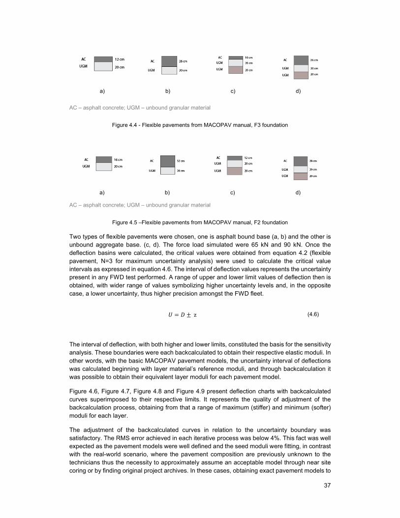
37

a) b) c) d)

AC – asphalt concrete; UGM – unbound granular material

Figure 4.4 - Flexible pavements from MACOPAV manual, F3 foundation

a) b) c) d)

AC – asphalt concrete; UGM – unbound granular material

Figure 4.5 –Flexible pavements from MACOPAV manual, F2 foundation

Two types of flexible pavements were chosen, one is asphalt bound base (a, b) and the other is unbound aggregate base. (c, d). The force load simulated were 65 kN and 90 kN. Once the deflection basins were calculated, the critical values were obtained from equation 4.2 (flexible pavement, N=3 for maximum uncertainty analysis) were used to calculate the critical value intervals as expressed in equation 4.6. The interval of deflection values represents the uncertainty present in any FWD test performed. A range of upper and lower limit values of deflection then is obtained, with wider range of values symbolizing higher uncertainty levels and, in the opposite case, a lower uncertainty, thus higher precision amongst the FWD fleet.

3 = + 4 z (4.6)

The interval of deflection, with both higher and lower limits, constituted the basis for the sensitivity analysis. These boundaries were each backcalculated to obtain their respective elastic moduli. In other words, with the basic MACOPAV pavement models, the uncertainty interval of deflections was calculated beginning with layer material’s reference moduli, and through backcalculation it was possible to obtain their equivalent layer moduli for each pavement model.

Figure 4.6, Figure 4.7, Figure 4.8 and Figure 4.9 present deflection charts with backcalculated curves superimposed to their respective limits. It represents the quality of adjustment of the backcalculation process, obtaining from that a range of maximum (stiffer) and minimum (softer) moduli for each layer.

The adjustment of the backcalculated curves in relation to the uncertainty boundary was satisfactory. The RMS error achieved in each iterative process was below 4%. This fact was well expected as the pavement models were well defined and the seed moduli were fitting, in contrast with the real-world scenario, where the pavement composition are previously unknown to the technicians thus the necessity to approximately assume an acceptable model through near site coring or by finding original project archives. In these cases, obtaining exact pavement models to

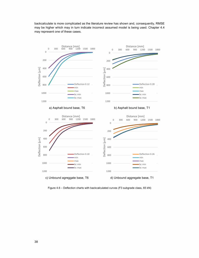
38

backcalculate is more complicated as the literature review has shown and, consequently, RMSE may be higher which may in turn indicate incorrect assumed model is being used. Chapter 4.4 may represent one of these cases.

a) Asphalt bound base, T6 b) Asphalt bound base, T1

c) Unbound agreggate base, T6 d) Unbound aggregate base, T1

Figure 4.6 – Deflection charts with backcalculated curves (F3 subgrade class, 65 kN)

0

200

400

600

800

1000

1200

0 300 600 900 1200 1500 1800

De

fle

ctio

n [

m]

Distance [mm]

Deflection 0.12

min

max

bc min

bc max

0

200

400

600

800

1000

1200

0 300 600 900 1200 1500 1800

De

fle

ctio

n [

m]

Distance [mm]

Deflection 0.28

min

max

bc min

bc max

0

200

400

600

800

1000

1200

0 300 600 900 1200 1500 1800

De

fle

ctio

n [

m]

Distance [mm]

Deflection 0.10

min

max

bc min

bc max

0

200

400

600

800

1000

1200

0 300 600 900 1200 1500 1800

De

fle

ctio

n [

m]

Distance [mm]

Deflection 0.26

min

max

bc min

bc max

39




0

200

400

600

800

1000

1200

0 300 600 900 1200 1500 1800

De

fle

ctio

n [

m]

Distance [mm]

Deflection 0.16

min

max

bc min

bc max

0

200

400

600

800

1000

1200

0 300 600 900 1200 1500 1800

De

fle

ctio

n [

m]

Distance [mm]

Deflection 0.32

min

max

bc min

bc max

0

200

400

600

800

1000

1200

0 300 600 900 1200 1500 1800

De

fle

ctio

n [

m]

Distance [mm]

Deflection 0.12

min

max

bc min

bc max

0

200

400

600

800

1000

1200

0 300 600 900 1200 1500 1800D

efl

ect

ion

[

m]

Distance [mm]

Deflection 0.28

min

max

bc min

bc max

40




0

200

400

600

800

1000

1200

0 300 600 900 1200 1500 1800

De

fle

ctio

n [

m]

Distance [mm]

Deflection 0.12

min

max

bc min

bc max

0

200

400

600

800

1000

1200

0 300 600 900 1200 1500 1800

De

fle

ctio

n [

m]

Distance [mm]

Deflection 0.28

min

max

bc min

bc max

0

200

400

600

800

1000

1200

0 300 600 900 1200 1500 1800

De

fle

ctio

n [

m]

Distance [mm]

Deflection 0.10

min

max

bc min

bc max

0

200

400

600

800

1000

1200

0 300 600 900 1200 1500 1800D

efl

ect

ion

[

m]

Distance [mm]

Deflection 0.26

min

max

bc min

bc max

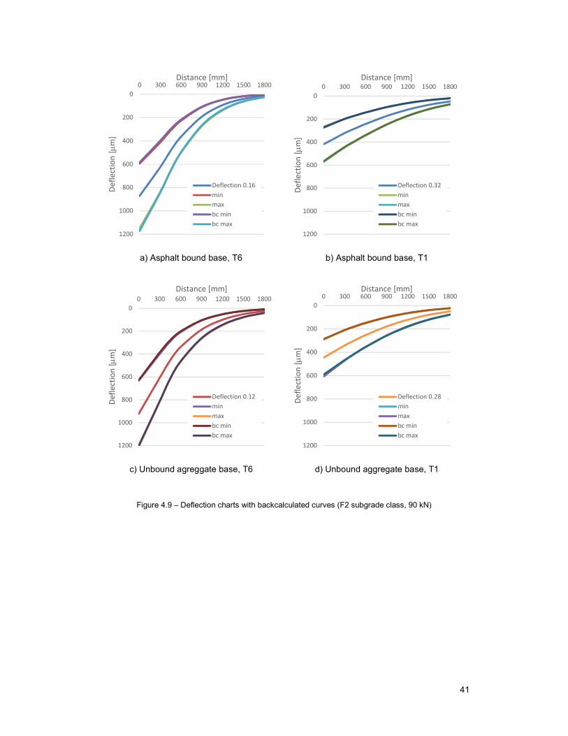
41




0

200

400

600

800

1000

1200

0 300 600 900 1200 1500 1800

De

fle

ctio

n [

m]

Distance [mm]

Deflection 0.16

min

max

bc min

bc max

0

200

400

600

800

1000

1200

0 300 600 900 1200 1500 1800

De

fle

ctio

n [

m]

Distance [mm]

Deflection 0.32

min

max

bc min

bc max

0

200

400

600

800

1000

1200

0 300 600 900 1200 1500 1800

De

fle

ctio

n [

m]

Distance [mm]

Deflection 0.12

min

max

bc min

bc max

0

200

400

600

800

1000

1200

0 300 600 900 1200 1500 1800D

efl

ect

ion

[

m]

Distance [mm]

Deflection 0.28

min

max

bc min

bc max

42

Table 4.2 and Table 4.3 resumes part of the backcalculated elastic moduli for the class F3 subgrade pavements subjected to 65 kN and 90 kN surface loads (see Appendix VII for all tables). It shows in a clear manner that the MACOPAV models presented convergent estimation of layer moduli for either 65 kN or 90 kN. In this way, the FWD fleet measurement uncertainty is now represented in the form of layer moduli, with the higher and the lower limits of the interval. In this form, it is possible to assess the range of moduli uncertainty when performing field surveys and even evaluate financially the same uncertainty although this study is outside the scope of the present dissertation.

Table 4.2 – Interval of pavement layer moduli, F3 subgrade class, 65 kN and 90 kN

Asphalt bound base, T6, 65 kN Asphalt bound base, T1, 65 kN

RMS 3.6% Reference RMS 0.9% RMS 3.6% Reference RMS 2.3%

Emax (1) E (2) Emin (3) Emax (1) E (2) Emin (3)

4700 4000 3000 4500 4000 3000 300 200 160 400 200 140 175 100 70 200 100 70

Asphalt bound base, T6, 90 kN Asphalt bound base, T1, 90 kN



4500 4000 3000 5000 4000 3500 300 200 180 390 200 150 165 100 70 190 100 75

Units in MPa; (1) – Layer modulus for stiffer limit layer composition; (2) – Reference layer moduli; (3) – Layer modulus for softer limit layer composition.

Table 4.3 – Interval of pavement layer moduli, F3 subgrade class, 65 kN and 90 kN

Unbound aggregate base, T6, 65 kN Unbound aggregate base T1, 65 kN



4300 4000 3300 5000 4000 3300 600 400 300 750 400 290 330 200 150 360 200 130 180 100 70 200 100 70

Unbound aggregate base T6, 90 kN Unbound aggregate base T1, 90 kN



4300 4000 3300 5000 4000 3300 600 400 300 700 400 290 310 200 150 360 200 130 160 100 70 190 100 70

Units in MPa; (1) – Layer modulus for stiffer limit layer composition; (2) – Reference layer moduli; (3) – Layer modulus for softer limit layer composition.

43

Figure 4.10 presents a final visual representation of the variation of each layer moduli. The variation in moduli values necessary to adjust the initial reference moduli to the critical values boundaries are expressed in function to the asphalt concrete material content in relation to the pavement total thickness (in percentage). From top to bottom, Top layer - Base - Sub-base - Subgrade, both the granular material layer required more adjustment, reaching as high as 80%, leading to stiffer layers for pavements with higher content of asphalt concrete (more than 40%). Pavement models with higher flexibility present higher sensitivity to FWD uncertainties.

a) Top layer

b) Base layer

c) Sub-base layer

d) Subgrade layer

Figure 4.10 – Variation in critical stiffness values in relation to percentage of asphalt concrete layer thickness over pavement’s total thickness

y = 0.00x + 0.06

R² = 0.45

y = -0.00x - 0.14

R² = 0.15

-100%

-80%

-60%

-40%

-20%

0%

20%

40%

60%

80%

100%

0 20 40 60 80 100

Asphalt layer thickness %

Top threshold

Bottom threshold

Variation in stiffness (Positive is stiffer)y = 0.01x + 0.41

R² = 0.29

y = 0.00x - 0.25

R² = 0,01.

-100%

-80%

-60%

-40%

-20%

0%

20%

40%

60%

80%

100%

0 20 40 60 80 100


Top threshold

Bottom threshold

Variation in stiffness (Positive is stiffer)

y = 0.01x + 0.37

R² = 0.70

y = -0.00x - 0.19

R² = 0.44

-100%

-80%

-60%

-40%

-20%

0%

20%

40%

60%

80%

100%

0 20 40 60 80 100


Top threshold

Bottom threshold


y = 0.00x + 0.69

R² = 0.04

y = 0.00x - 0.30

R² = 0.03

-100%

-80%

-60%

-40%

-20%

0%

20%

40%

60%

80%

100%

0 20 40 60 80 100


Top thresholdBottom threshold


44

4.4 Test site backcalculation

Regarding test site 1, the PTS results confirmed the findings included in chapter 4.3. The backcalculation of deflection measurements resulted in three different pavement designs, each influenced by the uncertainty already mentioned. In the event of a rehabilitation project, these results could directly affect the possible project solutions, namely when determining the necessary thickness of the overlay design, poising financial impacts on the project’s final cost.

Figure 4.11 and Figure 4.12 show deflection plot charts with BC deflection curve layered on top. RMSE obtained were between 6.0 to 8.4%. High RMSE values were obtained representing that the pavement model might not exactly match the actual pavement.

a) FWD 1 b) FWD 2

a) FWD 3

Figure 4.11 – Deflection chart with BC curve, Site 1, 65 kN

0

100

200

300

400

500

600

700

800

900

1 000

0 300 600 900 1200 1500 1800

De

fle

ctio

n [

m]

Distance [mm]

FWD 1

BC FWD 1

0

100

200

300

400

500

600

700

800

900

1 000

0 300 600 900 1200 1500 1800

De

fle

ctio

n [

m]

Distance [mm]

FWD 2

BC FWD 2

0

100

200

300

400

500

600

700

800

900

1 000

0 300 600 900 1200 1500 1800

De

fle

ctio

n [

m]

Distance [mm]

FWD 3

BC FWD 3

45

a) FWD 1 b) FWD 2

b) FWD 3

Figure 4.12 – Deflection chart with BC curve, Site 1, 90 kN

The AC top layer of just only 5 cm of thickness may also contribute to a less responsive model in BC software when adjusting such thin layer stiffness. In a different note, although test site 1 is an asphalt bound pavement, it was discovered that its asphalt content in the mix was not very significant which may modify its mechanical behavior when comparing to other proper asphalt mix pavements (see Appendix VIII).

Table 4.4 and Table 4.5 summarizes the Test Site 1 pavement model backcalculated moduli. FWD 1 clearly presents stiffer pavement estimation due to its lower deflection recordings. FWD 2 and 3 present moduli in similar value magnitude representing good reproducibility between the two, although no there are no information if both FWD tested with similar load pulse time.

0

100

200

300

400

500

600

700

800

900

1 000

0 300 600 900 1200 1500 1800D

efl

ect

ion

[

m]

Distance [mm]

FWD 1

BC FWD 1

0

100

200

300

400

500

600

700

800

900

1 000

0 300 600 900 1200 1500 1800

De

fle

ctio

n [

m]

Distance [mm]

FWD 2

BC FWD 2

0

100

200

300

400

500

600

700

800

900

1 000

0 300 600 900 1200 1500 1800

De

fle

ctio

n [

m]

Distance [mm]

FWD 3

BC FWD 3

46

In conclusion, the backcalculation of deflections measured independently by FWD 1, 2, 3 produced what can be considered an acceptable estimation of a multi-layer pavement model elastic moduli.

Table 4.4 – Backcalculation results for Site 1, 65 kN AC – Asphalt concrete; UGM - Unbound granular material; Root Mean Square Error (%)

Table 4.5 – Backcalculation results for Site 1, 90 kN

AC – Asphalt concrete; UGM - Unbound granular material; Root Mean Square Error (%)

4.5 Summary

Repeatability analysis for deflection measurement resulted in acceptable repeatability limits. In contrast, reproducibility analysis showed that the tested FWD could not reproduce each other’s deflection results within a reasonable reproducibility limit. Consequently, the sensitivity analysis for 95% confidence level were conducted with high standard deviation values which, in turn, resulted in wide critical value intervals. The interval of deflection values represents the range of upper and lower limit values of a random test performed by any given FWD in the fleet.

Standardized pavement models from MACOPAV (JAE, 1995) were used as reference base for the sensitivity analysis of backcalculated moduli. With standardized pavement models layer moduli backcalculated for both higher and lower stiffness uncertainty intervals, an analysis of the variation of each layer moduli from initial reference values in relation to asphalt concrete material in the pavement total thickness in percentage was performed to find which layer presented higher uncertainty under the backcalculation process. From top to bottom (Top layer - Base - Sub-base - Subgrade), both the granular material layer required more adjustments, as high as 80%, leading to estimated stiffer layers for pavements with higher content of asphalt concrete (more than 40%). Pavement models with higher AC percentage present higher sensitivity to FWD uncertainty. These BC estimated moduli RMSE were successfully kept under 4%. It also showed that the MACOPAV models presented a convergent estimation of layer moduli for either 65 kN or 90 kN. In this way, the FWD fleet measurement uncertainty is represented in the form of layer moduli, the higher and the lower limits of the interval, enabling a direct assessment of the range of moduli uncertainty when performing field surveys and even evaluating the financial implications although this study resides outside the scope of the present dissertation.

Layer Material Thickness

[cm] Seed

moduli FWD 1 FWD 2 FWD 3

Surface AC 5 4000 9500 6000 7000

Base UGM 20 900 600 600 500

Sub-base

Soil-cement 15 900 1200 600 900

Sandy soil 15 50 200 90 75

Sandy soil 100 30 40 50 40

RMS% 7.4 6.5 6.6

Layer Material Thickness

[cm] Seed

moduli FWD 1 FWD 2 FWD 3

Surface AC 5 4000 9000 6000 6500

Base UGM 20 900 700 600 650

Sub-base

Soil-cement 15 900 1200 600 600

Sandy soil 15 50 80 90 80

Sandy soil 100 30 45 60 50

RMS% 8.4 6.2 6.0

47

The sensibility analysis performed in this section portrays some of the uncontrollable and the randomly unknown factors that may influence the outcome of this study. There for it is crucial to be conservative while conducting these assessments.

49

5 Conclusion and recommendations

5.1 Summary

Pioneering campaigns such as the WASHO (1952-1954) (WASHO, 1954) and AASHO Road Test (1963) (AASHO, 1962) marked the beginning of the development of pavement engineering and also marked the beginning of the development of equipment for performing pavement tests. Prior to the 1930’s, road maintenance responsibility was attributed to the local authorities. Based on the literature review, road maintenance is viewed as being less favored than road design and construction. The focus shift from road maintenance to asset management (Madelin, 2000) motivated the development of testing methods capable of increasing network level campaigns efficiency. Non-destructive tests (NDT) became widely accepted as it enabled maintenance without resulting in road service disruption and avoided exposing workers to danger. Measuring deflections constitutes the simplest approach to evaluate qualitative parameters such as the bearing capacity of the sample. By applying a known force to the testing sample, we can measure how much it yields. To complete the characterization, physical properties can be determined by backcalculating deflection measurements, thus obtaining the wanted elastic moduli.

The objective of the present dissertation is to study the precision and uncertainty performance in FWD testing. This static impulse generating deflectometer is currently used as the standard deflection testing equipment (ASTM, 2009), mainly in point-to-point, project level, pavement testing campaigns. The FWD can measure the complete deflection bowl necessary to back calculate the multiple pavement layers underneath. The force pulse generated can simulate the action of a rolling wheel axel on the pavement. It is also significantly more mobile and easier to operate.

An experimental research in form of a proficiency test scheme (PTS), compliant with ISO/IEC 17043, organized under RELACRE, a fleet of three FWD were tested. An assessment of repeatability and reproducibility performance was performed. An uncertainty analysis followed allowing a better understanding of uncertainty’s influence to the quality of pavement structural capacity assessments, for example, in case of a structural quality evaluation to support a rehabilitation project. Lastly, a sensitivity analysis with standardized MACOPAV pavement models was also produced.

The experimental research results confirmed a satisfactory repeatability of deflection measurements. In contrast, the reproducibility is difficult to achieve in most cases. Consequently, the uncertainty levels revealed to be high. Uncertainty and precision revealed to be dependent of pavement type and deflection magnitude. Uncertainty presented high values for flexible pavement and for high deflections. Regarding to the sensitivity analysis on the uncertainty’s influence on the FWD results interpretation, it was concluded that the flexible pavements presented higher sensibility to uncertainty mainly when gauging for stiffness on the foundation layers.

5.2 Conclusions

The current dissertation allowed to find and aggregate several conclusions. Road and airfield pavement management is getting increasing attention in the engineering and business management fields as an opportunity to develop more technologically advanced and efficient methodologies to assess pavement condition at a network level, while enhancing the performance of the asset management in a competitive business sector. The practice has evolved from early XX century static or slow deflectometers to current developing traffic speed deflectometers, with

50

mobile computerized pavement condition assessment and data transfer to existing pavement management system.

The most used deflection measurement device is the FWD. The FWD is widely adopted by most road and airfield administrations to conduct routine pavement tests. Its popularity has promoted the existence of numerous peer reviewed articles and active regional user groups. In this scope, the proposed dissertation developed an experimental research featuring three FWD from different manufacturers (Dynatest, Carl Bro and KUAB). A proficiency test scheme developed to retrieve data from the FWD fleet to assess uncertainty’s influence on test results. The main conclusions were:

Repeatability and reproducibility limits result were dependent of deflection magnitude as well as pavement stiffness.

Repeatability limit for the flexible pavements test site was r=4 and for the rigid pavement test site r=2.

Reproducibility limits were higher and in function of any given deflection value. The trend line presented a steep slope, which towards the higher range of deflection presented the maximum reproducibility limit. For an assumed deflection of Df=300 nm, flexible pavement test site limit value was R=169 and for the rigid pavement test site, the limit value was R=93.

These results are in line with the reviewed literature (Garg, 2002; Murphy, 1998; Rocha et al, 2004) that thoroughly studies FWD repeatability and reproducibility. Although repeatability is normally achieved, reproducibility is dependent of ambient factors and each FWD feature, such as the deflectometer types, the analog-to-digital signal interpretation algorithm proprietary of each manufacturer, the quality of the rubber on the bottom of the loading plate, the shape and quality of the rubber buffers, the load pulse history, the drop height, the force frequency, and many other variables that make reproducibility hard to control effectively.

The accuracy of the pavement model determined for moduli backcalculation process play an important role in the success outcome of the analysis. Literature review indicate that loosely defined models produce high RMSE values which in turn poses difficulties to achieve correctly estimated layer moduli (Irwin, 2002). Reproducing pavement models exact to real location is difficult due to heterogeneity of layer properties and parameters in both in depth and longitudinally.

The backcalculation analysis performed under FWD uncertainty resulted in a range of interval for estimated moduli, representing the type of varying results that may be obtained attending to the reproducibility issues reported by literature. Backcalculation methods are not 100% straightforward and depends on several input parameters, such as the seed moduli, layer thickness, temperature, the pavement model, etc. The exercise of backcalculating MACOPAV pavement models produced a study of measured deflections that were backcalculated to layer moduli for two peak nominal loads, 65 and 90 kN. The result was a converging set of pavement layer moduli interval. These results can also, in turn, be used to evaluate uncertainty’s influence in proposed rehabilitation designs and the corresponded financial implications. The main conclusions were:

The adjustment of the backcalculated curves in relation to the uncertainty boundary was satisfactory. The RMS error achieved in each iterative process was below 4%.

51

The variation in moduli values necessary to adjust the initial reference moduli to the critical values boundaries were expressed in function to the asphalt concrete thickness in relation to the pavement total thickness (in percentage) and several conclusions were found:

o Granular layers required more adjustment, reaching as high as 80%, leading to stiffer layers for pavements with higher flexibility (more than 40%). Foundation layers also required more adjustment, around 80%, when adjusted to the uncertainty curves.

o Backcalculated moduli sensitivity to FWD uncertainties are directly linked to the pavement’s flexibility, i.e., highly flexible pavements are affected with higher uncertainty’s influence.

In conclusion, the initial objectives of the dissertation were accomplished. A repeatability and reproducibility analysis were successfully completed with data measured on site. This analysis was followed in an uncertainty assessment, which revealed that uncertainty was dependent of deflection values magnitude and pavement stiffness itself. Finally, the sensitivity analysis concluded that the more flexible the pavements presented the tendency to be more sensitive to FWD uncertainty.

5.3 Recommendations

As a final remark of this study several recommendations are suggested.

Both the literature review and the field trial provided evidence that FWD performance is bound to be influenced by random sources of uncertainty. To attain a satisfactory level of confidence, FWD operators should have a thorough understanding of the FWD functionalities and its operation principles. Environmental interferences such as the temperature’s effect on the pavement surface and the buffer system play some part in the accuracy variation. In addition, the interpretation of load time history (if allowed by the FWD model) and the acknowledgement of the high frequency cut off function are all requirements to provide a valid interlaboratory comparison and thus a better quality assessment in pavement engineering.

FWD operators should always be entitled to continuous training achieving better theoretical knowledge underlying routine operations.

The scope of this study did not contemplate the financial burden of poorly performed FWD analysis, such as backcalculating high uncertainty deflection measurements resulting in misleading pavement models subjected to rehabilitation project design. The author wishes to suggest this exercise from another opportunity of study which would be interesting and insightful. This opportunity would provide pavement engineers and decision makers with a sense of reality of the financial cost that could exist when calling for tender for new projects.

53

References

AASHO (1962). “The AASHO The road test”. American Association of State Highway and Transportation Officials, Washington, USA.

Alkasawneh, W. (2007). “Backcalculation of pavement moduli using genetic algorithms”. PhD dissertation. University of Akron. Ohio, USA.

Andersen, S., Levenberg, E., & Andersen, M. B. (2017). “Inferring pavement layer properties from a moving measurement platform”. BCRRA 2017 - 10th International Conference on the Bearing Capacity of Roads, Railways and Airfields. Athens, Greece.

Andrén, P. (2006). “Development and Results of the Swedish Road Deflection Tester”. Retrieved from http://www.diva-portal.org/smash/get/diva2:10556/FULLTEXT01.pdf. (Date Accessed: August 25, 2016)

Antonsen, V., & Mork, H. (2017). “A comparison of TSD and FWD deflections at Norwegian roads with an interpretation of bearing capacity from TSD measurements”. BCRRA 2017 - 10th International Conference on the Bearing Capacity of Roads, Railways and Airfields. Athens, Greece.

Antunes, M. L. (1997). “Desenvolvimento de modelos de degradação de pavimentos”. Colóquio sobre Conservação, Junta Autónoma de Estradas. Lisbon, Portugal

ASTM (1999). ASTM D6433-99 “Standard Practice for Roads and Parking Lots Pavement Condition Index Surveys”. ASTM International.

ASTM (2008). ASTM D4695–03 “Standard Guide for General Pavement Deflection Measurements”. ASTM International.

ASTM (2009). ASTM D4694-09 “Standard Test Method for Deflections with a Falling-Weight-Type Impulse Load”. ASTM International.

AUSTROADS (2006). “Guide to Asset Management Part 5E: Cracking”. Retrieved from https://www.onlinepublications.austroads.com.au/items/AGAM05E-06. (Date accessed: July 26, 2017).

AUSTROADS (2007a). “Guide to Asset Management Part 5B: Roughness”. Retrieved from https://www.onlinepublications.austroads.com.au/items/AGAM05B-07. (Date accessed: July 26, 2017).

AUSTROADS (2007b). “Guide to Asset Management Part 5C: Rutting”. https://www.onlinepublications.austroads.com.au/items/AGAM05C-07. (Date accessed: July 26, 2017).

AUSTROADS (2008). “Guide to Asset Management Part 5D: Strength”. Retrieved from https://www.onlinepublications.austroads.com.au/items/AGAM05D-08. (Date accessed: July 26, 2017).

AUSTROADS (2009a). “Guide to Asset Management Part 5F: Skid Resistance”. Retrieved from https://www.onlinepublications.austroads.com.au/items/AGAM05F-09. (Date accessed: July 26, 2017).

AUSTROADS (2009b). “Guide to Asset Management Part 5G: Texture”. Retrieved from https://www.onlinepublications.austroads.com.au/items/AGAM05G-09. (Date accessed: July 26, 2017).

AUSTROADS (2009c). “Guide to Pavement Technology Part 7: Pavement Maintenance”. Retrieved from https://www.onlinepublications.austroads.com.au/items/AGAM05C-07. (Date accessed: July 26, 2017).

54

AUSTROADS (2011). “Guide to Pavement Technology Part 5: Pavement Evaluation and Treatment Design”. Retrieved from https://www.onlinepublications.austroads.com.au/items/AGPT05-11. (Date accessed: July 26, 2017).

Benbow, E., & Wright, A. (2012). “HERoad (Holistic Evaluation of Road Assessment) Deliverable 1.1 – Pavement performance assessment”. Retrieved from http://vti.diva-portal.org/smash/get/diva2:814340/FULLTEXT01.pdf.

Bentsen, Nazarian, S., & Harrison. (1989). “Reliability Testing of Seven Nondestructive Pavement Testing Devices”. Nondestructive Testing of Pavements and Backcalculation of Moduli, STP 1026, pp. 41-58. American Society of Testing and Materials, Philadelphia, USA.

Bohn, A. O. (1989). “The History of the Falling Weight Deflectometer”. Retrieved from http://www.pavement-consultants.com/media/6042/HistoryOfFWD_AxelOBohn.pdf (Date accessed: August 9, 2016)

Branco, F., Pereira, P., & Picado Santos, L. (2008). “Pavimentos Rodoviários”. Edições Almedina. Coimbra, Portugal.

Brown, S. F., & Pappin, J. W. (1981). “Analysis of pavements with granular bases”. Transportation Research Record, 810, pp. 17-23.

Bush, J. A., & Baladi, G. Y. (1989). “Nondestructive testing of pavements and backcalculation of moduli”. International Symposium on Nondestructive Testing of Pavements and Backcalculation of Moduli, 1st, 1988, Baltimore, Maryland, USA.

Chen, D., Bilyeu, J., He, R., & Murphy, M. (1999). “Effects of Buffers on Falling Weight Deflectometer Measurements”. Internal Technical Memo, Design Pavement Section, TxDOT. Austin, Texas.

Choubane, B., Gokhale, S., Mike Jackson, N., & Nazef, A. (2006). “Assessing the Precision of Falling Weight Deflectometer for Field Measurements”. Journal of ASTM International, Vol. 3, No. 3, 2006, pp. 1-12.

Čičković, M. (2017). “Analysing FWD data — from the deflection bowl to material parameters”. BCRRA 2017 - 10th International Conference on the Bearing Capacity of Roads, Railways and Airfields. Athens, Greece.

Claessen, A., Edwards, J., Sommer, P., & Ugé, P. (1977). “Asphalt Pavement Design Manual: The SHELL Method”. University of Michigan. Michigan, USA.

Clarke, D. B., Harris, S. B., Heitzman, A. C., & Margiotta, R. A. (2003). “SHRP Long-Term Pavement Performance Information Management System”. Transportation Research Record 1260.

Correia, J. M. S. (2014). “Retro-análise de Resultados de Caracterização Estrutural de Pavimentos”. Dissertação de mestrado. Instituto Superior Técnico.

COST (1997). “COST 325 - New Road Monitoring Equipment and Methods. Final Report of the Action”. Directorate General Transport. European Comission.

COST (1998). “COST 336 – Information Gathering Report, Task Group 2 - FWD at Network Level”. Final draft report. European Comission.

Dormon, G. M. & Metcalf, C. T. (1965). “Design curves for flexible pavements based on layered system theory”. 43rd Annual Meeting of the Committee on Flexible Pavement Design.

Estradas de Portugal (1995). “Manual de Dimensionamento do Reforço de Pavimentos Flexíveis”. Estradas de Portugal.

European Commission. (2005). “FORMAT, Fully Optimised Road Maintenance, Final Technical Report”. European Commission.

55

Eurostat (n.d.-a). “Freight transport statistics - modal split”. Retrieved from http://ec.europa.eu/eurostat/statistics-explained/index.php/Freight_transport_statistics_-_modal_split. (Date accessed: April 8, 2017).

Eurostat (n.d.-b). “Trans-European networks in transport (TEN-T)”. Retrieved from http://ec.europa.eu/eurostat/statistics-explained/index.php/Trans-European_networks_in_transport_(TEN-T) . (Date accessed: April 8, 2017).

Fernando, E., Liu, W., & Ryu, D. (2001). “Development of a procedure for temperature correction of backcalculated AC modulus”. Texas: Texas Transportation Institute.

Fileccia Scimemi, G., Turetta, T., & Celauro, C. (2016). Backcalculation of airport pavement moduli and thickness using the Levy Ant Colony Optimization Algorithm. Construction and Building Materials, Vol. 119, pp. 288-295.

Flores, J. M., Van, P. Le, Park, C. K., Kim, W., & Lee, H. J. (2017). “Development of a frequency temperature correction model for FWD back-calculated moduli based on frequency-temperature superposition principle”. BCRRA 2017 - 10th International Conference on the Bearing Capacity of Roads, Railways and Airfields. Athens, Greece.

Fontul, S. (2004). “Strutural Evaluation of Flexible Pavements Using Non-Destrutive Tests”. Tese de Doutoramento. Departamento de Engenharia Civil. Universidade de Coimbra.

Francisco, A. (2012). “Comportamento estrutural de pavimentos rodoviários flexíveis”. Dissertação de Mestrado. Instituto Politécnico de Bragança.

Fwa, T., Chan, W., & Hoque, K. (2000). “Multiobjective optimization for pavement maintenance programming”. Journal of Transportation Engineering, 126 (5), pp. 367-374.

Garbowski, T., & Pożarycki, A. (2016). “Multi-level backcalculation algorithm for robust determination of pavement layers parameters”. Inverse Problems in Science and Engineering, Vol. 25 (5), pp. 674-693.

Garg, N. (2002). “Comparison between falling weight deflectometer and static deflection measurements on flexible pavements at the national airport pavement test facility (NAPTF)”. Federal Aviation Administration. Retrieved from airtech.tc.faa.gov/Pavement/Downloads/P-15.pdf. (Date accessed: April 24, 2017)

Goldberg, D. E. (1989). “Genetic Algorithms in Search, Optimization, and Machine Learning”. Addison-Wesley Professional. Reading, Massachusetts, USA.

Irwin, L. H. (2002). “Backcalculation : An Overview and Perspective”. FWD Backcalculation Workshop 3 – 6th International Conference on the Bearing Capacity of Roads, Railways and Airfields - BCRA 2002.

ISO (1994a). ISO 5725-1-1994 Accuracy (truness and precision) of measurement methods and results. International Organization of Standarization.

ISO (1994b). ISO 5725-2-1994 Accuracy (truness and precision) of measurement methods and results. International Organization of Standarization.

ISO (2010). ISO 17043-2010 Conformity assessment - General requirements for proficiency testing. International Organization of Standarization.

JAE (1995). “MACOPAV - Manual de Concepção e Pavimentos para a Rede Rodoviária Nacional”. Portugal.

JAE (1997). Catálogo de Degradações dos Pavimentos Rodoviários Flexíveis. Junta Autónoma de Estradas. Portugal.

Johnson, A. M. (2000). “Best Practice Handbook on Asphalt Pavement Maintenance”. Center for Transportation Studies, University of Minnesota. Minnesota, USA.

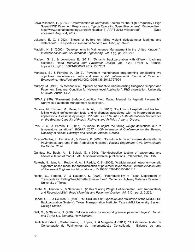
56

Leiva-Villacorta, F. (2012). “Determination of Correction Factors for the High Frequency / High Speed FWD Pavement Responses to Typical Operating Speed Responses”. Retrieved from http://www.asphalttechnology.org/downloads/(13)-AAPT-2012-Villacort.pdf. (Date accessed: August 4, 2017).

Lukanen, E. O. (1992). “Effects of buffers on falling weight deflectometer loadings and deflections”. Transportation Research Record, No. 1355, pp. 37-51.

Madelin, K. B. (2000). “Developments in Maintenance Management in the United Kingdom”. International Journal of Pavement Engineering, Vol. 1 (3), pp. 233-245.

Madsen, S. S., & Levenberg, E. (2017). “Dynamic backcalculation with different load-time histories”. Road Materials and Pavement Design, pp. 1-20. Taylor & Francis. https://doi.org/10.1080/14680629.2017.1307263

Meneses, S., & Ferreira, A. (2012). “Pavement maintenance programming considering two objectives: maintenance costs and user costs”. International Journal of Pavement Engineering. https://doi.org/10.1080/10298436.2012.727994

Murphy, M. (1998). “A Mechanistic-Empirical Approach to Characterizing Subgrade Support and Pavement Structural Condition for Network-level Application”. PhD dissertation. University of Texas, Austin, USA.

NPMA (1999). “Pavement Surface Condition Field Rating Manual for Asphalt Pavements”. Northwest Pavement Management Association.

Oshone, M., Elshaer, M., Dave, E., & Daniel, J. S. (2017). “Evolution of asphalt modulus from falling weight deflectometer tests and challenges associated with its interpretation and applications: A case study using LTPP data”. BCRRA 2017 - 10th International Conference on the Bearing Capacity of Roads, Railways and Airfields. Athens, Greece.

Pais, J. C., & Pereira, P. (2017). “A model to adjust the falling weight deflections due to temperature variations”. BCRRA 2017 - 10th International Conference on the Bearing Capacity of Roads, Railways and Airfields. Athens, Greece.

Picado-Santos, L., Ferreira, A., & Pereira, P. (2006). “Estruturação de um sistema de Gestão de Pavimentos para uma Rede Rodoviária Nacional”. Revista Engenharia Civil, Universidade Do Minho, No 26.

Quintus, H., Bush, A., & Baladi, G. (1994). “Nondestructive testing of pavements and backcalculation of moduli”. ASTM special technical publications. Phladelphia, PA. USA.

Rakesh, N., Jain, A. ., Reddy, M. A., & Reddy, K. S. (2006). “Artificial neural networks—genetic algorithm based model for backcalculation of pavement layer moduli”. International Journal of Pavement Engineering. https://doi.org/10.1080/10298430500495113

Rocha, S., Tandon, V., & Nazarian, S. (2001). “Reproducibility of Texas Department of Transportation Falling Weight Deflectometer Fleet”. Center for Highway Materials Research. University of Texas.

Rocha, S., Tandon, V., & Nazarian, S. (2004). “Falling Weight Deflectometer Fleet: Repeatability and Reproducibility”. Road Materials and Pavement Design, Vol. 5 (2), pp. 215-238.

Rohde, G. T., & Scullion, T. (1990). “MODULUS 4.0: Expansion and Validation of the MODULUS Backcalculation System”. Texas Transportation Institute, Texas A&M University System, College Station.

Salt, G., & Stevens, D. (2007). “Modular ratios for unbound granular pavement layers”. Tonkin and Taylor Ltd, Dunedin, New Zealand.

Santinho Horta, C., Costa Pereira, F., Lopes, S., & Morgado, J. (2011). “O Sistema de Gestão de Conservação de Pavimentos da Implementação Consolidada - Balanço de uma

57

Implementação Consolidada”. 7o Congresso Rodoviário Português. Lisboa, Portugal.

Shell (1995). “BISAR - User Manual”. Bitumen Business Group.

Sorensen, A. (1993). “Dynatest FWD/HWD field programs - smoothed (signal) peak option”. (Laboratorire Central des Points et Chaussées, Ed.), 2nd FWD Seminar of Forum of European National Highway Research Laboratories (FEHRL). Bouguenais: Laboratorire Central des Points et Chaussées.

Steer Davies Gleave. (2009). “Ex Post Evaluation of Cohesion Policy Programmes 2000-2006 Work Package 5A : Transport. First Intermediate Report”.

Tayabji, S., & Lukanen, E. O. (2000). “Nondestructive testing of pavements and backcalculation of moduli, Third Volume”. ASTM special technical publication. West Conshohocken, PA.

Van Gurp, C. (1991). “Consistency and Reproducibility of Falling Weight Deflections”. Road and Airport Pavement Response Monitoring Systems-Conference Proceedings, pp. 291-305. West Lebanon, New Hampshire, USA.

Van Gurp, C. (1995). “Characterization of seasonal influences on asphalt pavements with the use of falling weight deflectometers”. PhD dissertation. Technische Universiteit Delft.

WASHO (1954). “The WASHO Road Test”. National Research Council (U.S.). Highway Research Board.

Wright, A., Benbow, E., Spielhofer, R., Sjögren, L., Hildebrand, G., Kokot, D., Rabe, R. (2016). “Hi-SPEQ – Developing the Technical and Quality Requirements for High-speed Condition Surveys of Road Networks”. Transportation Research Procedia. https://doi.org/http://dx.doi.org/10.1016/j.trpro.2016.05.417

Zofka, A., Sudyka, J., & Sybilski, D. (2017). “Assessment of pavement structures at traffic speed”. BCRRA 2017 - 10th International Conference on the Bearing Capacity of Roads, Railways and Airfields. Athens, Greece.

59

Appendix

61

Appendix I. Proficiency test protocol

Ensaio de aptidão – 2016

Ensaio de carga com defletómetro de impacto (FWD)

Local dos ensaios: Depósito Geral de Material da Força Aérea Rua dos Pioneiros da Aviação 2615 – Alverca

Dia e hora: 6 de dezembro 2016 pelas 9:30

Informação a disponibilizar de cada entidade participante:

Nome dos técnicos presentes (portaria)

Matrícula da viatura (portaria)

Documento de identificação (portaria)

Comprovativo mais recente de calibração FWD (opcional)

Gama de tolerância dos geofones do respetivo aparelho (ou apresentar os dados técnicos completos)

Ano de fabrico/compra do equipamento (para aferir a sua geração)

Condições técnicas de realização dos ensaios:

1. Verificar as posições dos geofones 2. Verificar o diâmetro da placa de impacto 3. Medir a temperatura do ar e da superfície 4. Anotar os valores Load-pulse (sempre que possível) de cada ensaio de carga

Condições de realização dos ensaios:

Marcação do local onde assenta a placa de impacto e a orientação da régua com os geofones.

Diâmetro da placa de impacto: 30 cm

Posicionamento dos geofones:

D0 D1 D2 D3 D4 D5 D6 D7

D [mm] 0 300 450 600 900 1200 1500 1800

Tipo de pavimento Cargas a aplicar [kN] Número de repetições (registar todas)

Pavimento betuminoso 65, 90 2x (assentamento), 3x (repetibilidade)

Pavimento rígido 65, 90 2x (assentamento), 3x (repetibilidade)

Guia de procedimento:

Para cada entidade FWD e para cada amostra de pavimento: 1. Medição da temperatura no ar e no pavimento 2. Efetuar ensaio de carga:

i. 2x Pré-ensaios de carga para garantir o correto contacto da placa de impacto;

ii. 3x Ensaios de carga com captação da carga máxima gerada e dos valores das deflexões medidas. Registar dados carga-deflexão para calculo de Load-pulse quando possível.

Lisboa, 29 de outubro de 2016

63

Appendix I. FWD results

Table. I.1 - Site 1, 65 kN

Distance [mm] (Deflection [m])

Load [kN] PT 0 300 450 600 900 1200 1500 1800

FWD 1

1 65 24 534 388 319 262 178 133 104 88

2 65 24 533 387 318 261 178 132 104 88

TS 19 3 65 24 533 388 319 261 178 132 104 88

TA 22 A 533 388 319 261 178 132 104 88

FWD 2

1 65 (*) 707 544 448 371 262 198 160 140

2 65 (*) 711 545 450 372 262 198 158 140

TS 20 3 65 (*) 707 544 449 371 260 196 157 140

TA 21 A 708 544 449 371 261 197 158 140

FWD 3

1 65 24 764 572 462 383 268 203 164 142

2 65 24 764 566 459 385 276 217 156 147

TS 18 3 65 24 760 562 453 383 276 217 154 146

TA 20 A 763 567 458 383 273 212 158 145

TS – Surface temperature [oC], TA – Air temperature [oC], PT – Pulse time [ms], (*) – Not available



Load [kN] PT 0 300 450 600 900 1200 1500 1800

FWD 1

1 90 24 712 523 435 358 248 185 149 126

2 90 24 706 519 430 354 245 184 148 126

TS 18 3 90 24 711 522 435 356 248 186 150 127

TA 20 A 710 521 433 356 247 185 149 126

FWD 2

1 90 (*) 928 715 591 485 347 264 213 188

2 90 (*) 927 715 590 485 346 263 213 187

TS 20 3 90 (*) 929 718 593 486 345 264 216 188

TA 21 A 928 716 592 486 346 264 214 187

FWD 3

1 90 23 950 727 595 499 346 265 221 189

2 90 23 952 728 597 500 349 267 223 187

TS 19 3 90 23 953 731 599 501 352 270 223 189

TA 19 A 952 728 597 500 349 267 222 188


64



Load [kN] PT 0 300 450 600 900 1200 1500 1800

FWD 1

1 90 22 284 249 229 209 173 141 116 94

2 90 21 284 249 230 211 173 141 116 94

TS 17 3 90 22 284 249 229 210 173 141 116 95

TA 19 A 284 249 229 210 173 141 116 94

FWD 2

1 90 (*) 331 295 269 249 203 167 138 114

2 90 (*) 329 295 270 248 204 167 139 113

TS 17 3 90 (*) 331 296 271 247 204 168 137 114

TA 18 A 330 295 270 248 204 168 138 114

FWD 3

1 90 23 351 311 288 264 216 180 150 124

2 90 23 351 311 288 264 216 180 149 124

TS 17 3 90 23 351 311 288 264 217 180 149 124

TA 19 A 351 311 288 264 217 180 149 124


65

Appendix II. Smoothing filter test

Table. II.1 – Smoothing filter test results, Test site 1


LP PT SF Load 0 300 450 600 900 1200 1500 1800 Var %

3 23

60 Hz

65

625 406 323 255 166 117 89 74 11%

5 28 619 407 325 260 174 126 97 80 13%

7 31 605 402 325 262 178 129 99 82 9%

3 24

150 Hz

577 371 294 231 150 106 79 65

5 29 552 363 291 231 153 110 84 69

7 31 567 374 300 240 162 118 89 74

3 23

60 Hz

90

804 526 417 330 221 162 128 107 13%

5 28 836 554 446 359 247 182 142 118 14%

7 31 844 571 464 375 261 191 149 124 10%

3 23

150 Hz

726 470 373 295 195 142 112 93

5 27 738 486 391 315 216 159 125 102

7 30 778 522 422 341 235 172 134 110

LP – Number of load plates used which directly influence drop height, PT – Pulse time [ms], SF – Smoothing filter setting, Load – Nominal peak load [kN], Var % - Percentage variation of deflection when comparing results with SF set to 150 Hz and 60 Hz

Table. II.2 - Smoothing filter test results, LNEC rigid pavement


SF Load 0 300 450 600 900 1200 1500 1800 Var %

0 90 98% 98% 98% 98% 97% 97% 97% 99% 98%

60 Hz 90 105% 105% 105% 105% 104% 104% 104% 106% 105%

150 Hz 90 100% 100% 100% 100% 100% 100% 100% 100%

200 Hz 90 99% 99% 99% 99% 99% 99% 97% 101% 99%

SF – Smoothing filter setting, Load – Nominal peak load [kN], Var % - Percentage variation of deflection when comparing results with SF set to 150 Hz

67

Appendix III. Repeatability and Reproducibility, N=3

Table. III.1 – Cochran’s test

0 300 450 600 900 1200 1500 1800 Load

65 Flexible

OK FWD3*** FWD3* OK FWD3* FWD3*** FWD3* FWD3*** OK

90 Flexible

OK OK OK OK OK OK FWD2* OK OK

90 Rigid FWD2*** FWD2*** OK OK OK FWD2*** OK OK OK

OK – Accept, * - Suspect outlier (95%), ** - Reject outlier (99%), *** - Suspect (95%) and Reject outlier (99%)

Table. III.2 - Grubb’s test

0 300 450 600 900 1200 1500 1800 Load

65 Flexible

OK OK OK OK OK OK OK OK OK

90 Flexible


90 Rigid OK OK OK OK OK OK OK OK OK


Table. III.3 - Site 1, 65 kN

0 300 450 600 900 1200 1500 1800

X 668.20 499.60 408.60 338.80 237.50 180.60 140.10 124.30

119.99 97.52 77.96 67.37 51.91 42.52 31.26 31.56

r2 4.22 8.67 7.44 0.67 7.56 22.33 10.11 2.33

d2 43189.59 28533.17 18231.80 13617.77 8082.50 5425.01 2932.29 2989.01

L2 14395.12 9508.17 6074.78 4539.03 2691.5 1800.89 974.06 995.56

R2 14399.34 9516.83 6082.23 4539.70 2699.20 1823.22 984.17 997.89

CVr 0.3% 0.6% 0.7% 0.2% 1.2% 2.6% 2.3% 1.2%

CVR 18.0% 19.5% 19.1% 19.9% 21.9% 23.6% 22.4% 25.4%

r 5.82 8.33 7.72 2.31 7.78 13.37 9.00 4.32

R 339.59 276.08 220.71 190.68 147.03 120.84 88.78 89.40

X – mean of means, - standard deviation, r2 – repeatability variance, d

2 - intralaboratory variance, L2

– interlaboratory variance, R2 - repeatability variance, CVr – repeatability coefficient of variation, CVR –

reproducibility variance, r – repeatability, R – reproducibility

68


0 300 450 600 900 1200 1500 1800

X 863.10 655.30 540.50 447.10 314.00 238.70 195.10 167.40

133.40 116.25 92.91 79.24 58.04 46.51 40.14 35.62

r2 4.56 3.89 4.89 1.78 4.33 2.56 1.78 0.67

d2 53390.30 40542.08 25897.10 18835.29 10107.00 6489.98 4833.39 3807.17

L2 17795.25 13512.73 8630.74 6277.84 3367.56 2162.47 1610.54 1268.83

R2 17799.80 13516.62 8635.62 6279.62 3371.89 2165.03 1612.32 1269.50

CVr 0.2% 0.3% 0.4% 0.3% 0.7% 0.7% 0.7% 0.5%

CVR 15.5% 17.7% 17.2% 17.7% 18.5% 19.5% 20.6% 21.3%

R 6.04 5.58 6.26 3.77 5.89 4.52 3.77 2.31

R 377.57 329.02 262.99 224.26 164.33 131.68 113.63 100.83

X – Mean of means, - standard deviation, r2 – repeatability variance, d

2 - intralaboratory variance- L2


reproducibility variance, r – repeatability, R – reproducibility, IC 95% - critical value for IC 95% normal distribution, IC 80% - critical value for IC 80% normal distribution


0 300 450 600 900 1200 1500 1800

X 321.80 285.10 262.40 240.70 197.70 162.80 134.40 110.70

34.31 32.23 30.07 27.74 22.27 19.89 16.93 15.08

r2 0.44 0.11 0.44 0.67 0.22 0.11 0.44 0.22

d2 3530.60 3117.09 2713.10 2308.01 1488.08 1187.00 860.30 682.28

L2 1176.72 1038.99 904.22 769.11 495.95 395.63 286.62 227.35

R2 1177.16 1039.10 904.66 769.78 496.17 395.74 287.06 227.57

CVr 0.2% 0.1% 0.3% 0.3% 0.2% 0.2% 0.5% 0.4%

CVR 10.7% 11.3% 11.5% 11.5% 11.3% 12.2% 12.6% 13.6%

r 1.89 0.94 1.89 2.31 1.33 0.94 1.89 1.33

R 97.10 91.23 85.12 78.52 63.04 56.30 47.95 42.69





69

Appendix IV. Repeatability and Reproducibility, N=2

Table. IV.1 – Cochran’s test

0 300 450 600 900 1200 1500 1800 Load

65 Flexible

OK FWD3* OK OK OK FWD3* OK FWD3*** OK

90 Flexible


90 Rigid FWD2*** FWD2*** FWD2*** FWD2*** OK FWD2*** OK FWD2*** OK


Table. IV.2 - Grubb’s test

0 300 450 600 900 1200 1500 1800 Load

65 Flexible


90 Flexible


90 Rigid OK OK OK OK OK OK OK OK OK


Table. IV.3 - Site 1, 65 kN

0 300 450 600 900 1200 1500 1800

X 735.70 555.50 453.50 377.50 267.30 204.80 158.20 142.50

38.679 15.839 6.364 8.768 8.485 10.607 0.212 3.536

r2 6.17 12.83 11.00 0.83 11.33 33.33 15.17 3.50

d2 4488.15 752.64 121.50 230.64 216.00 337.50 0.15 37.50

L2 747.00 123.30 18.42 38.30 34.11 50.69 -2.50 5.67

R2 753.16 136.13 29.42 39.13 45.44 84.03 12.66 9.17

CVr 0.3% 0.6% 0.7% 0.2% 1.3% 2.8% 2.5% 1.3%

CVR 3.7% 2.1% 1.2% 1.7% 2.5% 4.5% 2.2% 2.1%

r 7.0 10.1 9.4 2.6 9.5 16.3 11.0 5.3

R 77.7 33.0 15.3 17.7 19.1 25.9 10.1 8.6

X – mean of means, - standard deviation, r2 – repeatability variance, d

2 - intralaboratory variance, L2


reproducibility variance, r – repeatability, R – reproducibility

70


0 300 450 600 900 1200 1500 1800

X 939.90 722.40 594.20 492.70 347.50 265.50 218.20 188.00

16.758 8.980 4.031 10.394 2.121 2.546 5.869 0.424

r2 1.67 3.67 3.17 0.67 5.00 3.33 2.17 0.83

d2 842.55 241.95 48.75 324.15 13.50 19.44 103.35 0.54

L2 140.15 39.71 7.60 53.91 1.42 2.68 16.86 -0.05

R2 141.81 43.38 10.76 54.58 6.42 6.02 19.03 0.78

CVr 0.1% 0.3% 0.3% 0.2% 0.6% 0.7% 0.7% 0.5%

CVR 1.3% 0.9% 0.6% 1.5% 0.7% 0.9% 2.0% 0.5%

R 3.7 5.4 5.0 2.3 6.3 5.2 4.2 2.6

R 33.7 18.6 9.3 20.9 7.2 6.9 12.3 2.5






0 300 450 600 900 1200 1500 1800

X 340.70 303.20 279.00 256.00 210.00 173.70 143.70 118.90

14.637 11.102 12.728 11.314 8.910 8.980 7.990 7.283

r2 0.67 0.17 0.50 0.50 0.33 0.17 0.67 0.17

d2 642.75 369.75 486.00 384.00 238.14 241.95 191.55 159.15

L2 107.01 61.60 80.92 63.92 39.63 40.30 31.81 26.50

R2 107.68 61.76 81.42 64.42 39.97 40.46 32.48 26.66

CVr 0.2% 0.1% 0.3% 0.3% 0.3% 0.2% 0.6% 0.3%

CVR 3.0% 2.6% 3.2% 3.1% 3.0% 3.7% 4.0% 4.3%

r 2.3 1.2 2.0 2.0 1.6 1.2 2.3 1.2

R 29.4 22.2 25.5 22.7 17.9 18.0 16.1 14.6





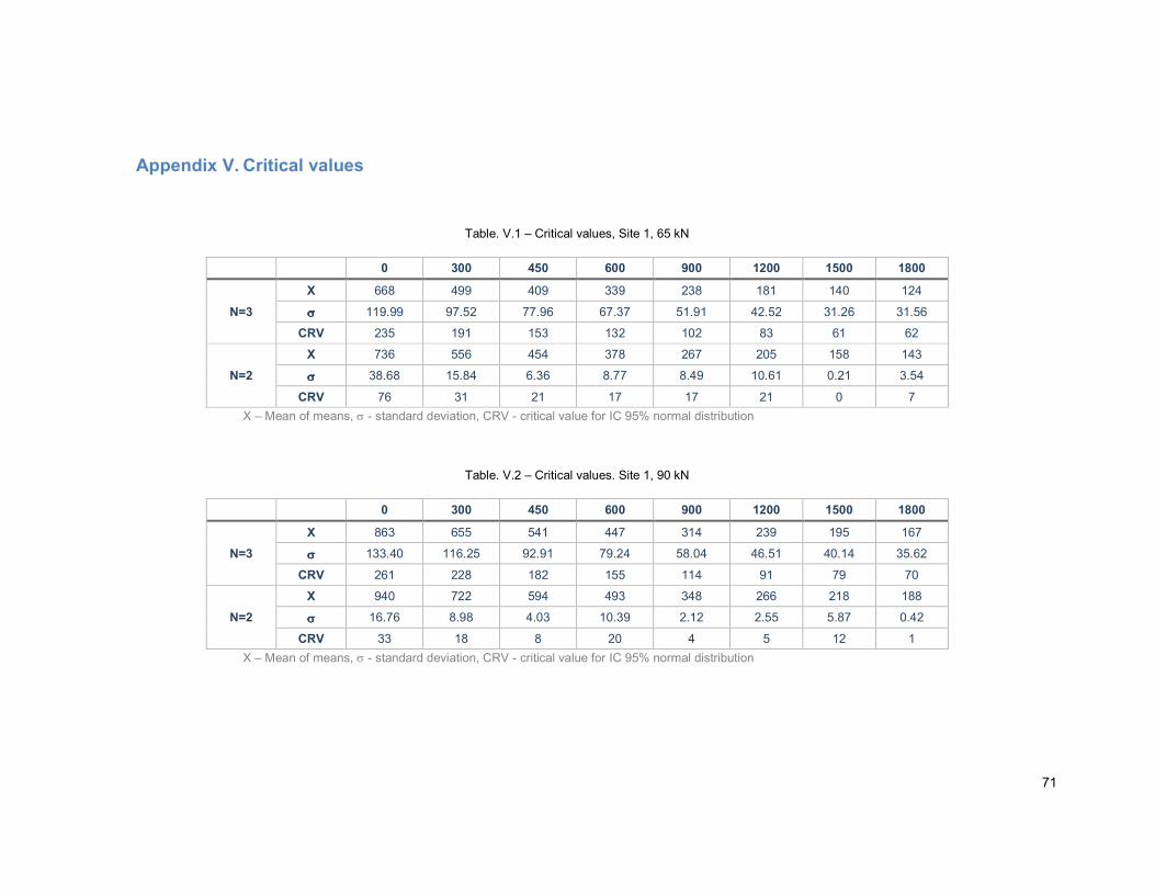
71

Appendix V. Critical values

Table. V.1 – Critical values, Site 1, 65 kN

0 300 450 600 900 1200 1500 1800

N=3

X 668 499 409 339 238 181 140 124

119.99 97.52 77.96 67.37 51.91 42.52 31.26 31.56

CRV 235 191 153 132 102 83 61 62

N=2

X 736 556 454 378 267 205 158 143

38.68 15.84 6.36 8.77 8.49 10.61 0.21 3.54

CRV 76 31 21 17 17 21 0 7

X – Mean of means, - standard deviation, CRV - critical value for IC 95% normal distribution

Table. V.2 – Critical values. Site 1, 90 kN

0 300 450 600 900 1200 1500 1800

N=3

X 863 655 541 447 314 239 195 167

133.40 116.25 92.91 79.24 58.04 46.51 40.14 35.62

CRV 261 228 182 155 114 91 79 70

N=2

X 940 722 594 493 348 266 218 188

16.76 8.98 4.03 10.39 2.12 2.55 5.87 0.42

CRV 33 18 8 20 4 5 12 1


72

Table. V.3 – Critical values, Site 2, 90 kN

0 300 450 600 900 1200 1500 1800

N=3

X 322 285 262 241 198 163 134 111

34.31 32.23 30.07 27.74 22.27 19.89 16.93 15.08

CRV 67 63 59 54 44 39 33 30

N=2

X 341 303 279 256 210 174 144 119

14.64 11.10 12.73 11.31 8.91 8.98 7.99 7.28

CRV 29 22 25 22 17 18 16 14


73

Appendix VI. Pavement structures

Table. VI.1 – Reference layer moduli

Pavement type Pavement model Reference moduli

F3, asphalt bound

base

AC 4000

UGM 200

Subgrade 100

RL 1000

F3, asphalt bound

base

AC 4000

UGM 200

Subgrade 100

RL 1000

F3, unbound

aggregate base

AC 4000

UGM 400

UGM 200

Subgrade 100

RL 1000

F3, unbound

aggregate base

AC 4000

UGM 400

UGM 200

Subgrade 100

RL 1000

F2, asphalt bound

base

AC 4000

UGM 120

Subgrade 60

RL 1000

F2, asphalt bound

base

AC 4000

UGM 120

Subgrade 60

RL 1000

F2, unbound

aggregate base

AC 4000

UGM 240

UGM 120

Subgrade 60

RL 1000

74

Pavement type Pavement model Reference moduli

F2, unbound

aggregate base

AC 4000

UGM 240

UGM 120

Subgrade 60

RL 1000

AC -asphalt concrete, UGM – unbound granular material, RL – rigid layer, Measuring unit - MPa

75

Appendix VII. Backcalculation of pavement structures

Table. VII.1 - F3, asphalt bound base 0.12, 65 kN Deflection Dlow Dhigh BClow Emax BChigh Emin

0 593 390 796 391 4700 809 3000

300 360 224 496 217 300 500 160

450 249 148 350 142 175 352 70

600 170 96 244 92 3000 244 600

900 77 38 116 38 4700 116

1200 34 14 55 15 55

1500 16 5 26 5 26

1800 8 2 14 2 14

RMS% 3.6 0.9


0 273 164 382 176 4500 382 3000

300 198 114 282 115 400 281 140

450 166 93 238 92 200 237 70

600 137 75 199 73 2500 197 600

900 89 45 133 43 130

1200 55 25 85 24 82

1500 33 13 52 13 50

1800 19 6 31 6, 30

RMS% 3.6 2.3

Table. VII.3 - F3, unbound granular base 0.10, 65 kN Deflection Dlow Dhigh BClow Emax BChigh Emin

0 513 332 694 335 4300 691 3300

300 296 180 412 173 600 412 300

450 211 123 300 118 330 299 150

600 154 86 223 83 180 221 70

900 84 42 126 42 3500 124 600

1200 46 20 72 21 70

1500 25 9 41 10 40

1800 14 4 23 4 23

RMS% 2.8 1.5

Table. VII.4 - F3, unbound granular base 0.26 Deflection Dlow Dhigh BClow Emax BChigh Emin

0 260 156 365 157 5000 354 3300

300 186 106 265 103 750 260 290

450 156 87 224 83 360 220 130

600 129 70 188 67 200 185 70

900 87 44 129 42 3000 127 600

1200 56 26 87 25 84

1500 36 15 57 15 55

1800 22 8 36 8 35

RMS% 3.6 2.5

Units: Deflection m, Elastic modulus: MPa; Deflection – simulated deflection measurement, Dlow – lower critical interval for deflections, Dhigh – upper critical interval for deflections, BClow – backcalculated deflection for lower CI, BChigh – backcalculated deflection for upper CI, Emax – estimated moduli for lower CI, Emin – estimated moduli for upper CI

76


0 629 416 842 421 4800 846 3000

300 449 287 612 285 200 607 90

450 348 216 480 214 100 471 45

600 262 157 367 156 2700 356 580

900 138 75 201 76

191

1200 66 32 101 33

94

1500 28 11 46 12

43

1800 10 3 18 3

18

RMS% 3.9

3.9


0 303 185 421 198 5000 408 3200

300 232 137 328 144 200 319 90

450 203 118 288 122 110 281 40

600 175 99 251 103 3000 245 750

900 125 67 183 69

178

1200 85 43 127 44

123

1500 55 25 85 26

82

1800 34 14 54 14

51

RMS% 3.9

3.2


0 665 442 888 437 4500 867 3500

300 439 279 598 267 380 586 175

450 328 202 454 192 190 444 90

600 244 145 344 139 105 334 45

900 135 73 196 72 3500 188 550

1200 72 35 109 36

104

1500 37 15 59 16

56

1800 18 6 30 6

29

RMS% 3.3

3.2


0 322 198 446 201 5000 440 3000

300 246 146 346 144 440 339 190

450 213 124 301 121 220 295 90

600 182 104 260 101 115 253 45

900 128 69 187 68 2500 182 450

1200 87 44 130 44

127

1500 56 26 87 27

86

1800 35 14 56 15

56

RMS% 2.8

2.0


77


0 821 557 1086 558 4500 1120 3000

300 499 322 675 312 310 692 180

450 345 214 476 206 165 487 70

600 235 139 331 134 2750 338 800

900 107 56 157 56

160

1200 48 21 74 22

76

1500 22 8 36 8

37

1800 11 3 19 3

20

RMS% 4.0

2.7


0 378 237 519 238 5000 529 3500

300 274 165 383 160 390 388 150

450 229 135 324 129 190 328 75

600 189 108 270 103 2400 272 700

900 123 66 180 63

180

1200 76 37 115 36

114

1500 45 20 70 20

69

1800 26 10 42 10

41

RMS% 3.5

1.2


0 710 475 945 484 4300 957 3300

300 410 259 561 258 600 571 300

450 293 178 407 178 310 414 150

600 213 124 302 126 160 306 70

900 117 62 172 65 3500 172 600

1200 64 30 98 32

97

1500 35 14 55 15

55

1800 19 6 31 6

32

RMS% 3.9

1.0


0 361 225 497 225 5000 489 3300

300 257 154 361 148 700 360 290

450 215 126 305 120 360 305 130

600 179 102 256 97 190 256 70

900 120 64 176 62 2500 176 700

1200 78 38 117 38

117

1500 49 22 77 23

76

1800 31 12 49 13

49

RMS% 3.9

0.7


78

Table. VII.13– F2, asphalt bound base 0.16, 90 kN Deflection Dlow Dhigh BClow Emax BChigh Emin

0 871 594 1148 584 4800 1172 3000

300 622 411 833 396 200 840 110

450 481 310 653 297 100 652 45

600 362 226 499 216 2500 493 800

900 191 110 273 106

264

1200 92 47 137 47

131

1500 39 17 62 17

60

1800 14 4 24 4

25

RMS% 3.5

2.9

Table. VII.14 – F2, asphalt bound base 0.32, 90 kN Deflection Dlow Dhigh BClow Emax BChigh Emin

0 419 265 572 274 5000 565 3000

300 322 198 446 199 180 442 100

450 281 170 392 170 90 390 50

600 242 144 341 142 2000 339 500

900 173 98 248 96

246

1200 118 63 173 60

171

1500 76 37 115 36

113

1800 47 21 73 19

71

RMS% 3.6

1.7

Table. VII.15 – F2, unbound granular base 0.12, 90 kN Deflection Dlow Dhigh BClow Emax BChigh Emin

0 921 631 1211 627 4500 1200 3500

300 607 400 814 386 360 812 175

450 454 290 618 279 185 615 90

600 338 209 467 202 100 463 45

900 187 107 266 105 3000 261 550

1200 100 52 148 52

144

1500 51 23 79 24

78

1800 25 9 40 9

41

RMS% 2.9 1.7

Table. VII.16 – F2, unbound granular base 0.28, 90 kN Deflection Dlow Dhigh BClow Emax BChigh Emin

0 446 285 608 289 5000 591 3500

300 341 211 471 209 400 466 170

450 295 179 410 176 200 408 85

600 252 150 353 147 110 354 40

900 178 101 254 99 2500 257 650

1200 120 64 176 63

179

1500 78 39 118 38

120

1800 49 22 75 22

77

RMS% 1.6 1.8


79

Table. VII.17 - Sensitivity analysis, Percentage of top layer over pavement total thickness

F3, 65 kN F3, 90 kN F2, 65 kN F2, 90 kN

Asp

halt

bo

un

d b

ase

0.12m Top Bottom 0.12m Top Bottom 0.16m Top Bottom 0.16m Top Bottom

4000 18% -25% 4000 13% -25% 4000 20% -25% 4000 20% -25%

200 50% -20% 200 55% -10% 120 67% -25% 120 67% -8%

100 75% -30% 100 65% -30% 60 67% -25% 60 67% -25%


4000 13% -25% 4000 25% -13% 4000 25% -20% 4000 25% -25%

200 100% -30% 200 95% -25% 120 67% -25% 120 50% -17%

100 100% -30% 100 90% -25% 60 83% -33% 60 50% -17%

13% -25%

Un

bo

un

d g

ran

ula

r b

ase


4000 8% -18% 4000 8% -18% 4000 13% -13% 4000 13% -13%

400 50% -25% 400 50% -25% 240 58% -27% 240 50% -27%

200 65% -25% 200 55% -25% 120 58% -25% 120 54% -25%

100 80% -30% 100 60% -30% 60 75% -25% 60 67% -25%


4000 25% -18% 4000 25% -18% 4000 25% -25% 4000 25% -13%

400 88% -28% 400 75% -28% 240 83% -21% 240 67% -29%

200 80% -35%

200 80% -35%

120 83% -25%

120 67% -29%

100 100% -30%

100 90% -30%

60 92% -25%

60 83% -33%

Units: Elastic modulus: MPa; Top – upper threshold (softer layer), Bottom – lower threshold – (stiffer layer)

81

Appendix VIII. Test site 1 backcalculation

Table. VIII.1 – Test site 1 backcalculation

FWD 1, 65 kN Deflection BC E Thickness

0 534 593 6500 0.050

300 388 364 650 0.200

450 319 299 700 0.150

600 262 252 110 0.150

900 178 181 60 1.000

1200 133 131 200

1500 104 95

1800 88 70

RMS% 9.3


0 712 737 7000 0.050

300 523 475 850 0.200

450 435 398 700 0.150

600 358 340 150 0.150

900 248 250 60 1.000

1200 185 184

1500 149 136

1800 126 102

RMS% 8.8


0 708 746 6000 0.050

300 544 492 600 0.200

450 449 418 600 0.150

600 371 363 90 0.150

900 261 277 50 1.000

1200 197 215

1500 158 168

1800 140 134

RMS% 6.5


0 928 992 6000 0.050

300 716 643 600 0.200

450 591 542 600 0.150

600 485 469 90 0.150

900 346 358 60 1.000

1200 264 277

1500 214 219

1800 188 176

RMS% 6.2


0 763 813 7000 0.050

300 566 534 500 0.200

450 458 449 600 0.150

600 384 388 75 0.150

900 273 293 40 1.000

1200 212 223

1500 158 171

1800 145 133

RMS% 6.1


0 952 991 6500 0.050

300 729 661 650 0.200

450 597 560 600 0.150

600 500 485 80 0.150

900 349 368 50 1.000

1200 267 282

1500 222 218

1800 188 172

RMS% 6.0

Units: Deflection m, Elastic modulus: MPa, Layer thickness: m; Deflection – measured “in-situ” deflection, BC – backcalculated deflection, E – estimated moduli, thickness – Layer thickness

82

Figure. VIII.1 - Backcalculated deflections (65 kN and 90 kN)

0

100

200

300

400

500

600

700

800

900

1 000

0 300 600 900 1200 1500 1800

De

fle

ctio

n [

m]

Distance [mm]

FWD 1

BC FWD 1

0

100

200

300

400

500

600

700

800

900

1 000

0 300 600 900 1200 1500 1800

De

fle

ctio

n [

m]

Distance [mm]

FWD 1

BC FWD 1

0

100

200

300

400

500

600

700

800

900

1 000

0 300 600 900 1200 1500 1800

De

fle

ctio

n [

m]

Distance [mm]

FWD 2

BC FWD 2

0

100

200

300

400

500

600

700

800

900

1 000

0 300 600 900 1200 1500 1800

De

fle

ctio

n [

m]

Distance [mm]

FWD 2

BC FWD 2

0

100

200

300

400

500

600

700

800

900

1 000

0 300 600 900 1200 1500 1800

De

fle

ctio

n [

m]

Distance [mm]

FWD 3

BC FWD 3

0

100

200

300

400

500

600

700

800

900

1 000

0 300 600 900 1200 1500 1800

De

fle

ctio

n [

m]

Distance [mm]

FWD 3

BC FWD 3

Non-destructuve tests in roads and airfields A study of ...

Documents

Transcript of Non-destructuve tests in roads and airfields A study of ...