Node-based analysis of species distributions

Acc

epte

d A

rtic

le

This article has been accepted for publication and undergone full peer review but has not

been through the copyediting, typesetting, pagination and proofreading process, which may

lead to differences between this version and the Version of Record. Please cite this article as

doi: 10.1111/2041-210X.12283

This article is protected by copyright. All rights reserved.

Received Date : 13-May-2014 Revised Date : 17-Sep-2014 Accepted Date : 23-Sep-2014 Article type : Research Article Editor : Robert B. O'Hara

Node-based analysis of species

distributions

Michael K. Borregaard†1,2

, Carsten Rahbek2, Jon Fjeldså

2, Juan Parra

3, Robert J. Whittaker

1,2

and Catherine H. Graham4

† Corresponding author: Michael K. Borregaard, email: [email protected]

Affiliations:

1. Conservation Biogeography and Macroecology Programme, Oxford University Centre for

the Environment, University of Oxford, South Parks Road, OX1 3QY, Oxford, United

Kingdom.

2. Center for Macroecology, Evolution and Climate, Natural History Museum of Denmark,

University of Copenhagen, Universitetsparken 15, 2100 Copenhagen Ø, Denmark.

3. Instituto de Biología, Facultad de Ciencias Exactas y Naturales, Universidad de Antioquia,

Medellín, Colombia.

4. Stony Brook University, 650 Life Sciences Building, Stony Brook, New York 11789, USA.

Running title: Node-based analysis of clade distribution

mailto:[email protected]

mailto:[email protected]

Acc

epte

d A

rtic

le


MS submitted to Methods in Ecology and Evolution in the 'standard paper' category.

Summary

1. The integration of species distributions and evolutionary relationships is one of the most

rapidly moving research fields today, and has led to considerable advances in our

understanding of the processes underlying biogeographical patterns. Here, we develop a set

of metrics, the specific overrepresentation score (SOS) and the geographic node divergence

(GND) score, which together combine ecological and evolutionary patterns into a single

framework, and avoids many of the problems that characterise community phylogenetic

methods in current use.

2. This approach goes through each node in the phylogeny, and compares the distributions of

descendant clades to a null model. The method employs a balanced null model, is

independent of phylogeny size, and allows an intuitive visualisation of the results.

3. We demonstrate how this novel implementation can be used to generate hypotheses for

biogeographical patterns with case studies on two groups with well-described

biogeographical histories: a local-scale community dataset of hummingbirds in the North

Andes, and a large-scale dataset of the distribution of all species of New World flycatchers.

The node-based analysis of these two groups generates a set of intuitively interpretable

patterns that are consistent with current biogeographical knowledge.

4. Importantly, the results are statistically tractable, opening many possibilities for their use in

analyses of evolutionary, historical and spatial patterns of species diversity. The method is

implemented as an upcoming R package nodiv, which makes it accessible and easy to use.

Acc

epte

d A

rtic

le


Key-words: allopatry, bird biogeography, distribution, evolution, macroecology,

macroevolution, null model, phylogeny, R, range.

Introduction

It has long been recognized that evolutionary and ecological processes interact to generate

patterns of species diversity (Wallace 1876). The recent explosion of data on species

distributions and phylogenetic relationships has made it possible to study these processes

quantitatively and has led to the development of new analytical techniques. Studies

integrating species distributions and phylogenetic relationships have used two distinct

approaches: site-based approaches, which use phylogenies to answer questions about how the

species of communities are related to each other; and clade-based approaches, which compare

the spatial distributions of individual clades. Although using the same data, the two

approaches focus on distinct sets of questions and have largely separate literatures.

Site-based metrics quantify spatial variation in the relatedness of co-occurring

species and include measures of community phylogenetic structure (e.g., the net relatedness

index (NRI), Webb et al. 2002), phylogenetic diversity (Faith 1994) and phylogenetic beta-

diversity (Graham & Fine 2008). The basic approach is to calculate a summary metric for all

species within each site, describing the phylogenetic relatedness of the species, using e.g. the

amount of shared branch length or the average phylogenetic distance among species. These

metrics have been interpreted in the context of factors such as local competitive exclusion

and habitat specialisation. Clade-based approaches focus on comparing specific clades by

quantifying spatial overlap between sister clades. These analyses are usually undertaken at

larger scales, and have been used to answer questions about the importance of allopatry in the

process of speciation (Barraclough & Vogler 2000; Fitzpatrick & Turelli 2006).

Acc

epte

d A

rtic

le


Both approaches have become widely used in evolutionary ecology. However,

concerns have been raised that the apparent simplicity of site-based metrics such as NRI,

which derives from reducing the complexity of relationships across an entire phylogeny to a

single, seemingly interpretable value (Webb et al. 2008), may in fact obscure the underlying

complexity of processes and may thus be misleading. For instance, Parra et al. (2010)

demonstrated that some assemblages with neutral NRI values, ostensibly indicating

phylogenetically random community assembly, were composed of a mosaic of closely related

and distantly related species. This suggests an alternative interpretation, namely that opposing

processes of phylogenetic exclusion and filtering take place at different phylogenetic scales.

As a solution, they proposed a null model approach using the nodesig algorithm from the

software Phylocom, which compares the species richness of each node to that expected from

randomly drawing species from the phylogeny (Webb et al. 2008). Parra et al. (2010) used

nodesig to analyse a phylogeny of hummingbirds from local assemblages in Northern

Ecuador, and demonstrated a complex spatial pattern of clade overrepresentation. Further

analysis showed that sites with overrepresentation of specific clades were spatially and

environmentally segregated, indicating that environmental adaptations or isolation of certain

clades are responsible for the spatial distribution of species within the group.

Here, we develop a measure of clade overrepresentation that we term the

‘specific overrepresentation score’ (SOS), which combines the clade-based and site-based

approaches. This measure is related to the metric of Parra et al. (2010), but takes a clade-

based approach by comparing the species richness of sister clades, rather than comparing

each clade to the total phylogeny. This means that the SOS is unaffected by how the

phylogeny is delimited, i.e. a hummingbird clade has the same SOS value in a study of all

birds and a study comprising only hummingbirds. The algorithm goes through each node,

corresponding to a pair of sister clades in the phylogeny, and compares the species richness

Acc

epte

d A

rtic

le


of the two clades in each community to the expectation from a null model. The result is a

matrix of SOS values for each combination of nodes and communities. These values can be

mapped geographically for each node, offering a visual representation of the degree of

distributional divergence among sister clades.

All SOS values calculated for a certain node can be summarized across

occupied sites to yield the 'geographic node divergence' (GND), which quantifies the

distributional divergence between the two daughter lineages descending from a given node.

The GND score thus identifies which nodes are responsible for observed patterns of

phylogenetic structure and species co-occurrence. Contrasting the nodes identified using

GND with those identified by macroevolutionary analyses could provide insight into factors

structuring diversity patterns. For instance, comparison of the nodes identified by GND with

those where there are changes in diversification rate, or in trait evolution, may facilitate the

exploration of the geographic and environmental context of morphological innovations (Parra

et al. 2010; Beaulieu et al. 2012). In addition, if a time-tree is available, analyses based on

GND permit the exploration of relationships between nodes of interest and events in earth

and/or climate history. We suggest that the GND metric provides a statistically tractable basis

for a unified understanding of the historical mechanisms influencing extant patterns of

biological diversity.

To exemplify the approach, we calculate SOS and GND scores for two well-

studied groups of Neotropical birds, each of which has a different scale of spatial resolution.

We show how the GND scores highlight nodes that identify evolutionary divergences

associated with distributional separation. We also show how mapping SOS values may serve

as a basis for further analysis of the biogeography of the group. Finally, we demonstrate how

the method can be extended to environmental space, providing a useful tool for exploring the

evolution of environmental associations within a clade. Our goal is to use these case studies

Acc

epte

d A

rtic

le


to demonstrate the method, rather than to provide an extensive account of the biogeographic

history of the groups analysed.

Materials and Methods

Calculating SOS

The SOS corresponding to a given node in a given site is calculated by comparing the species

richness of each daughter clade to random assemblages created by a null model (Fig. 1). Null

assemblages are created by extracting all species descending from the focal node and then

randomizing their occurrences among all occupied sites. This procedure maintains the

richness pattern of the focal node, but randomizes the relative distributions of its two

daughter clades.

To avoid biasing null communities by oversampling rare species, the null model must

control for differences in species occupancy. The correct way of doing this has been

vigorously debated (Gotelli & Graves 1996), but the current consensus is that the best method

is random matrix swapping, which swaps occurrences randomly among species in the

community matrix while maintaining the species richness of sites, and the range size of

species, as constant properties (Gotelli 2000; Gotelli & Entsminger 2003). These swap

algorithms remove any systematic pattern of species co-occurrence, which makes them well

suited for evaluating ecological or phylogenetic processes determining species co-occurrence.

However, the procedure is computationally intensive, even using efficient algorithms such as

the ‘quasiswap’ algorithm (Miklós & Podani 2004), implemented as a C routine within the R

(v 3.0) package ‘vegan’ (Oksanen et al. 2012) (v 2.0-7).

Repeating the randomization procedure n times creates a distribution of

expected richness values for each daughter clade. From this distribution we can extract two

Acc

epte

d A

rtic

le


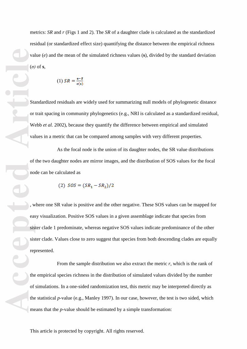
metrics: SR and r (Figs 1 and 2). The SR of a daughter clade is calculated as the standardized

residual (or standardized effect size) quantifying the distance between the empirical richness

value (e) and the mean of the simulated richness values (s), divided by the standard deviation

(σ) of s,

(1)

Standardized residuals are widely used for summarizing null models of phylogenetic distance

or trait spacing in community phylogenetics (e.g., NRI is calculated as a standardized residual,

Webb et al. 2002), because they quantify the difference between empirical and simulated

values in a metric that can be compared among samples with very different properties.

As the focal node is the union of its daughter nodes, the SR value distributions

of the two daughter nodes are mirror images, and the distribution of SOS values for the focal

node can be calculated as

, where one SR value is positive and the other negative. These SOS values can be mapped for

easy visualization. Positive SOS values in a given assemblage indicate that species from

sister clade 1 predominate, whereas negative SOS values indicate predominance of the other

sister clade. Values close to zero suggest that species from both descending clades are equally

represented.

From the sample distribution we also extract the metric r, which is the rank of

the empirical species richness in the distribution of simulated values divided by the number

of simulations. In a one-sided randomization test, this metric may be interpreted directly as

the statistical p-value (e.g., Manley 1997). In our case, however, the test is two sided, which

means that the p-value should be estimated by a simple transformation:

Acc

epte

d A

rtic

le


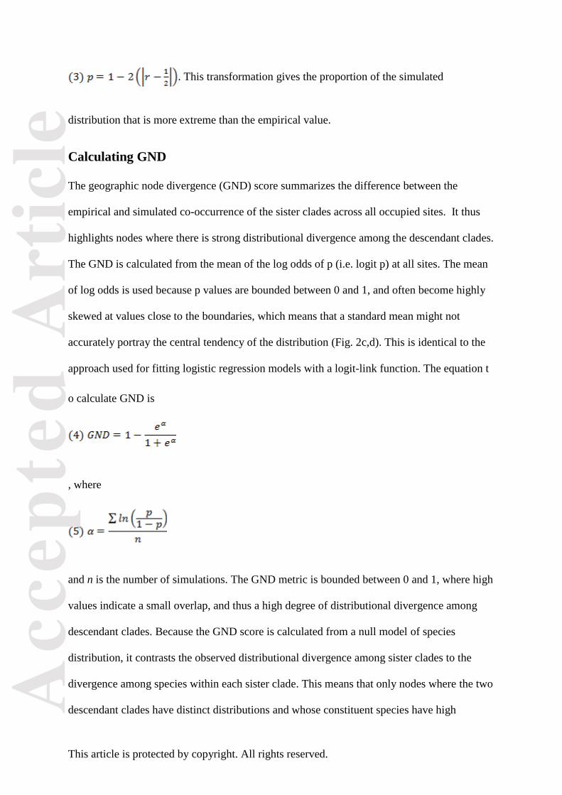
. This transformation gives the proportion of the simulated

distribution that is more extreme than the empirical value.

Calculating GND

The geographic node divergence (GND) score summarizes the difference between the

empirical and simulated co-occurrence of the sister clades across all occupied sites. It thus

highlights nodes where there is strong distributional divergence among the descendant clades.

The GND is calculated from the mean of the log odds of p (i.e. logit p) at all sites. The mean

of log odds is used because p values are bounded between 0 and 1, and often become highly

skewed at values close to the boundaries, which means that a standard mean might not

accurately portray the central tendency of the distribution (Fig. 2c,d). This is identical to the

approach used for fitting logistic regression models with a logit-link function. The equation t

o calculate GND is

, where

and n is the number of simulations. The GND metric is bounded between 0 and 1, where high

values indicate a small overlap, and thus a high degree of distributional divergence among

descendant clades. Because the GND score is calculated from a null model of species

distribution, it contrasts the observed distributional divergence among sister clades to the

divergence among species within each sister clade. This means that only nodes where the two

descendant clades have distinct distributions and whose constituent species have high

Acc

epte

d A

rtic

le


distributional overlap are highlighted.

SOS/GND scores in environmental space

The approach described here is based on species occurrences in geographic assemblages;

however, the analysis can be extended to environmental variables. We do this by gridding the

environmental space; i.e. we divide the environmental variables into equal-sized bins, and

tally the occurrences of species in each bin to form an environment-by-species matrix. The

node-based analysis can then be applied to the environment-by-species matrix, to calculate

SOS and GND in environmental bins. This makes it possible to identify nodes where

important changes in the occupancy of environmental conditions arise, as we demonstrate in

the hummingbird case study below. By comparing the geographic node-based analysis to the

environmental node-based analysis, it is also possible to determine if geographic changes are

associated with changes in environmental conditions.

The relationship between climate variables and SOS values can be modelled using

regression analysis, which should be especially useful for evaluating the effect of larger

numbers of independent climatic factors. Another approach for expanding the enviromental

analysis is to first fit an environmental niche mode to each species, and then apply the

binning procedure to the modeled niches, as if they were continuous ranges. This should

create smoother relationships between climate variables and SOS, and resolve the issue that

bin sizes are arbitrary. Note, though, that the use of environmental niche models is debated

and entails a number of important assumptions which complicates the analysis (Araújo &

Guisan 2006).

Simulation study

We exemplify the approach and behaviour of the metrics using a pair of simulated sister

clades. Each simulated clade consisted of S circular ranges, each with a radius of 15 grid cells

Acc

epte

d A

rtic

le


(giving a geographic range size of ~479 grid cells). The midpoint of each range was placed

randomly around the central point of the associated clade according to an uncorrelated

bivariate normal distribution, where the variation of range placement was determined by the

standard deviation, i.e. , where X and Y are the coordinates of

the central point of the clade, is the standard deviation, I is the identity matrix, and N2 is the

bivariate normal distribution. The standard deviation describes the overlap of ranges of

species within the same sister clade. The simulation domain was 100x100 grid cells, large

enough to ensure that no ranges came into contact with the domain edges.

To assess the sensitivity of the GND metric to clade divergence, we varied the

distance between the central points of the two sister clades from 0 to 30, simulating clades at

all values in the interval (0, 1, 2, … 30). The maximum distance of 30 grid cells corresponds

to a very slight overlap between sister clades, at the given range radius of 15 units. To

demonstrate the effect of the range overlap within each sister clade (controlled by the

standard deviation, ) and clade size (S), we reran the simulation at high and low values of

these parameters. Within-clade species overlap was simulated as standard deviation values of

2 and 10 grid cells, corresponding to very high and very low within-clade overlap. Clade size

was simulated using values of 10 and 100 species in each sister clade. Using 200 replicates

for each parameter combination, this resulted in 24,800 individual simulation runs.

To achieve this high level of replication, we used the rdtable algorithm in R to create

null communities. This algorithm is several orders of magnitude more efficient than the

‘quasiswap’, but can lead to slightly inaccurate results, in that rdtable may yield matrices

with elements other than 0 and 1. This will create increased variation in simulated richness

values and may lead to underestimation of absolute SOS values (i.e. the bias makes the test

Acc

epte

d A

rtic

le


for divergence more conservative). To evaluate the size of this potential bias, we also

conducted 5 replicates for 12 different parameter combinations using the quasiswap

algorithm and compared the results.

Case study datasets

The interpretation of SOS and GND values depend to some extent on the spatial scale. At

larger extents and grain sizes, the analysis mainly detects biogeographical events, such as

movement among biomes or continents, whereas local community analysis can be interpreted

in the context of metacommunity dynamics and phylogenetic changes of environmental

preference, where clades move into and radiate (or persist) in new environments. To illustrate

the potential applications of the method we used two datasets that differ in spatial grain and

extent: a large-scale dataset of gridded range maps for New World flycatchers, and a

community dataset of individual hummingbird assemblages in the Northern Andes.

The large-scale dataset consists of range maps of all species of New World

flycatchers (family Tyrannidae in the traditional sense; now subdivided into several families,

see Ohlson et al. 2013). The range maps were taken from the Copenhagen database of bird

distributions (originally collated by Rahbek & Graves 2001). This database provides 1° x 1°

resolution range maps of all birds of the world, and is continuously updated. We extracted

the data on the 26th

of June 2012. Phylogenetic information for the 390 species of New World

flycatchers was extracted from a super-tree of all the world’s birds (see Holt et al. 2012 for

references), which incorporates a recently revised phylogeny of the Tyrannidae (Ohlson et al.

2013).

The second dataset includes 219 hummingbird (Trochilidae) assemblages

containing 126 species across Ecuador and Colombia. This dataset was used in Graham et al.

(2012), and 108 of the species were used in the analysis by Parra et al. (2010). See Graham et

Acc

epte

d A

rtic

le


al. (2012) for details on the approach taken in compiling the dataset. Our molecular

phylogeny of hummingbirds included each of the 126 hummingbird species evaluated in this

study and is described in Graham et al. (2009).

We also extracted the mean annual temperature and total annual precipitation at

each locality in the hummingbird dataset from Worldclim (Hijmans et al. 2005). The

environmental data were grouped into bins of 2 °C for temperature and 400 mm/yr for

precipitation. For simplicity we used the raw locality climate data for this comparison, rather

than fitting an environmental niche model. The size of the bins were chosen to ensure an even

number of bins for temperature and precipitation, a high number of occurrences in each bin

(range 0 to 40), and good compliance with the precision of the environmental variables (i.e.

no bins should be completely empty along the entire axis of either temperature or

precipitation).

R package 'nodiv'

All codes and functions necessary to calculate GND and SOS scores is made available in the

R package 'nodiv', which should be available on GitHub and CRAN from October 2014. The

package integrates with data formats from the existing and widely successful packages 'ape'

and 'picante', and provides functions to calculate the scores, and to perform plots with maps

of SOS values and phylogenies with GND scores, similar to the figures presented here.

Results

Simulations

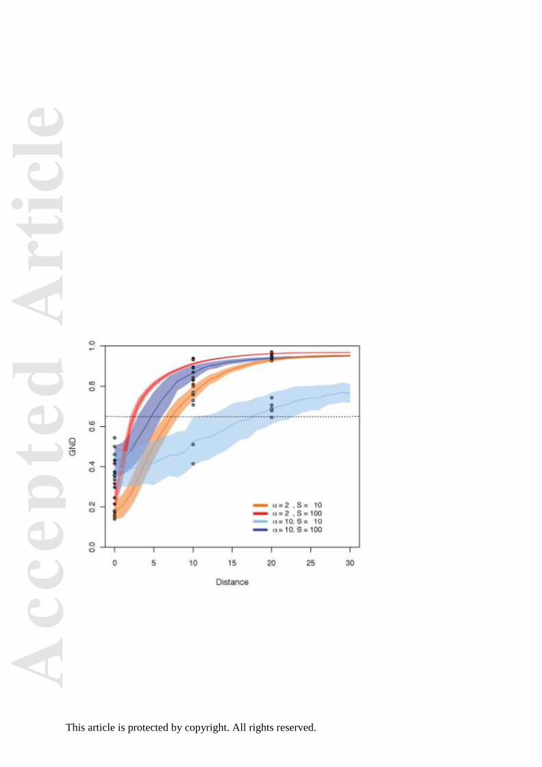
In the simulations, GND values for most clades increased rapidly with increasing distance

between the distributional centres of sister clades (Fig. 3). In the case of high standard

Acc

epte

d A

rtic

le


deviation (8 units) and small species numbers (10 per sister clade) the GND increased only

slowly, which is the expected behaviour of the metric: GND scores contrast the overlap of

two clades to the overlap of ranges within each clade, and so GND scores are smaller when

species within each sister clade have low distributional overlap. Standard deviations of 8–10

units are realistic: the standard deviation among sister clades of New World flycatchers range

from 0 to 30 grid cells and vary with the number of species in clades (Fig. S1),

notwithstanding that the empirical range sizes are mostly smaller than those in the simulated

data set (Fig. S2). GND values greater than 0.65 were consistently associated only with

clades that were clearly geographically divergent, and we suggest this value as a rule-of-

thumb threshold for identifying interesting nodes in the phylogeny. The results based on the

more computationally intensive quasiswap algorithm were broadly consistent with the results

using rdtable (Fig. 3), indicating that the simulations give an accurate representation of the

behaviour of GND.

New World flycatchers

The New World flycatchers comprise a number of small clades and two species-rich clades,

the Rhynchocyclidae (consisting of the Pipriomorphines, Todi Tyrants and allies) and

Tyrannidae sensu strictu (Ohlson et al. 2013). The GND scores reveal that major

distributional divergences are restricted to a relatively small number of nodes (Fig. 4). Here,

we focus on six nodes in the phylogeny that exhibit GND scores above 0.65, corresponding

to major distributional shifts in flycatcher assemblages (Figs 4 and 5). The nodes with the

highest GND scores primarily occur along the lineage leading to the present-day Fluvicolinae

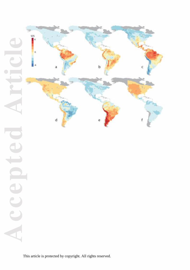
(Fig. 4). The most basal of these nodes (node A) corresponds to the split between the

Rhynchocyclidae and the Tyrannidae. The spatial pattern of SOS values (Fig. 5a) illustrates

the geography of this divergence, with the Rhynchocyclidae being over-represented in the

lowland rain forest biomes, whereas the Tyrannidae are widely distributed across all of South

Acc

epte

d A

rtic

le


and North America. The second highlighted node splits the Elaenines, which are over-

represented in the Andean region and the open savannah of eastern South America, from the

rest of the group (node B in Figs 4 and 5). The node with the highest GND score (C)

separates the tyrant flycatchers (Tyranninae) from the Fluvicolines. The tyrant flycatchers are

primarily distributed in tropical lowland forests but extend to the surrounding savannahs and

southern North America; whereas the Fluvicolines inhabit colder and drier environments, and

extend to the subarctic zones at the poleward tips of South and North America. Within the

Fluvicolines, node D (Figs 4 and 5d) separates a small basal group of species, associated with

the subtropical and upland savannah biomes characterizing the eastern and northern parts of

South America, from the rest of the clade. The remaining Fluvicolines are split (at node E in

Figs 4 and 5e) into a group that inhabit Andean cloud-forest and woodlands and barren

habitats in the southern cone of the continent and a second group of species associated with

montane to boreal forest habitats distributed across the Central Andes and into North

America. The final node exhibiting strong distributional change (F in Figs 4 and 5) is a

relatively young node (below the genus level), which separates kingbirds (Tyrannus)

occurring in South America from those in North America.

Hummingbird assemblages

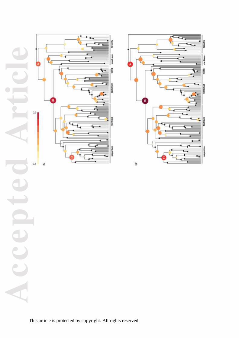
Three nodes in the regional hummingbird phylogeny exhibit a high degree of node allopatry,

indicating distributional segregation among the hummingbird assemblages of the northern

Andes (Fig. 6a). These same three nodes feature prominently in the analyses based on

environmental bins (Figs 6b and S3). The most basal of the nodes (Fig. 6a node A) represents

the phylogenetic split between the hermits and all other hummingbird clades (except topazes,

which are basal to the hermits). The geographic distribution of SOS values show that this

node corresponds to a distributional segregation between species assemblages in lowland

Amazonia (dominated by hermits) and all other clades, which are broadly distributed across

Acc

epte

d A

rtic

le


the region (Fig. 7a left).

For the environmental analysis, values of mean annual temperature were binned

This geographic result is mirrored by the environmental analysis, whereby hermits are

confined to wet and warm regions, while all other clades occur across a broad range of

environmental conditions (Figs 6b node A and 7a right). The node with highest node

allopatry score in both the geographic (Fig. 6a node B) and environmental analyses (Fig. 6b

node B) represents the split between the Andean high elevation brilliants and coquettes, and

the mangoes, bees and emeralds (Fig. 7b left). Brilliants and coquettes have radiated within

the Andes (Bleiweiss 1998a, b; McGuire et al. 2007), and occupy environmental conditions

of cold temperatures (i.e. high elevation) and intermediate levels of precipitation, while the

mangoes, bees and emeralds occur in mid- and low- elevation sites that are warmer but have

varied precipitation conditions (Fig. 7b right). The final highlighted node (C in Fig. 6)

represents a split within the coquettes, and separates high and mid-elevation species within

the Andes (Fig. 7c left and right).

Discussion

Here, we show that the SOS/GND approach has the potential to be a powerful tool for

integrating phylogenetic and spatial information into a statistically tractable framework. The

GND identifies key locations within a phylogeny where clades differ in their geographic

distribution or environmental associations. GND scores are comparable among nodes in a

phylogeny, and between different phylogenies, making it possible to estimate the timing and

prevalence of major distributional shifts. Furthermore, maps of SOS depict the geographic

context of a given shift, and together with the environmental analysis yield insight into the

congruence between geographic and environmental divergences in the phylogeny. Because

of these characteristics, the approach should afford a more complete understanding of the

Acc

epte

d A

rtic

le


phylogenetic structure of assemblages than that offered by whole-tree phylogenetic indices

commonly used in community phylogenetics (cf. Parra et al. 2010).

The SOS/GND approach complements several related approaches that attempt

to explicitly connect evolutionary patterns within phylogenies with spatial patterns across

regions or assemblages (e.g., Leibold et al. 2010). For instance, ancestral area analysis aims

to use present-day distributions to model the likely distributional history of a clade (Ree et al.

2005). In contrast, the GND score is simply a metric to quantify the degree of distributional

divergence among sister clades. As such, GND does not require the geographical

distributions of species to be defined a priori as distinct allopatric units. This allows the use

of this technique for groups such as the Tyrannidae where clades are partially sympatric. Also,

the philosophical underpinnings of the techniques are quite different: ancestral area

reconstruction models geographical distribution as a trait that evolves at a certain rate across

the phylogeny. This implicitly assumes that range dynamics are slow enough to be modelled

as evolutionary traits, and that the ancestral distribution of clades must have been within the

current distributional range. This property makes the ancestral area reconstruction method

inapplicable for e.g. local community or metacommunity data, and it is, possibly, also

unrealistic for analysing continental-scale range dynamics. The approach presented here is

also distinct from traditional clade-based comparisons, such as the metric for node overlap

developed by Barraclough & Vogler (2000), in explicitly linking the pattern to community

patterns, and in taking a probabilistic approach. Thus, the SOS/GND method not only

computes the distributional overlap between clades, but also controls for the number of co-

occurring species, and for the degree of distributional overlap within clades.

The usefulness of our approach is demonstrated by our two case studies. For the

New World flycatchers, the analysis reveals that the current pattern of species distributions is

the result of major distributional divergences at a relatively small number of nodes. Most

Acc

epte

d A

rtic

le


nodes with high GND scores are basal in the phylogeny and correspond to the division

between large taxonomic groups of Tyrannidae, which likely diversified in the late Oligocene

to mid-Miocene (Ohlson et al. 2013). Three general patterns characterize the highlighted

nodes. The clearest pattern is one of splits between clades over-represented in wet and warm

tropical environments (Amazonia, Central America and the Atlantic forest of Brazil) and

clades over-represented in seasonal environments with open forest structures (Figs 5a and 5c).

Two other characteristic patterns are splits between clades over-represented in the lowlands

versus the Andes (Figs 5b, 5c, 5d and 5e) and splits between clades over-represented in North

vs. South America (Figs 5e and 5f). These results are consistent with the hypothesis that

distributional shifts into novel habitats have been followed by local in-situ radiations, as

suggested by Ohlson et al. (2008). Importantly, our analyses provide an objective statistical

basis for identifying the nodes where particularly large changes in distribution patterns

occurred.

The community-scale analysis of hummingbirds also identifies relatively few

nodes associated with large geographic shifts. There are three nodes associated with clades

crossing the transition between high-elevation and low-elevation zones, a phenomenon that

occurs in many avian lineages (Ribas et al. 2007; Sedano & Burns 2010; Chaves et al. 2011).

The environmental analysis identifies most of the same nodes, indicating that adaptations to

new environments may have led to subsequent radiation in the topographically complex

Andean mountains (García-Moreno et al. 1999; Weir 2006; Fjeldså & Irestedt 2009). This

process is demonstrated by the inferred movement of Brilliants and Coquettes into the Andes,

a feature of our analysis which is consistent with several lines of evidence that these groups

colonised montane environments and diversified in these regions (Bleiweiss 1998a, b).

Mangos, whose origin cannot be confidently attributed to either the lowlands or highlands

(McGuire et al. 2007), also show a distributional and environmental shift where one clade of

Acc

epte

d A

rtic

le


mangos seems to have moved into high elevations. Again, these results are in accordance

with existing knowledge on biogeographic patterns of hummingbird distribution (Bleiweiss

1998a, b; McGuire et al. 2007; Graham et al. 2009), but express them in a transparent

statistical framework.

While the patterns found for hummingbirds in this study are consistent with the

findings of Parra et al. (2010), there are a number of important differences. Parra et al. (2010)

simply identified patterns of over-representation, whereas we defined specific

overrepresentation scores (SOS) that are comparable across analyses and standardised for

species richness and geographic occupancy. We also calculated GND scores, allowing us to

identify where significant distributional shifts occurred in the evolution of the clade.

Parra et al. (2010) identified 21 significantly over-represented nodes, many of

which were nested in the phylogeny and corresponded to the same geographic sites. The

explanation for this pattern is that the algorithm used by Parra et al. (2010) compares the

species richness pattern of a node to that of the basal node of the phylogeny used in a given

study (Webb et al. 2008). With their approach, all nodes that are over-represented with

respect to the basal node will be highlighted, which means that daughter nodes of over-

represented nodes will also tend to be over-represented. This makes it difficult to identify

which nodes are associated with major distributional changes. For instance, a single

distributional change, such as a long-distance dispersal event, may lead to a pattern where all

nodes descending from that node will come out as over-represented; and possibly also some

nodes that are ancestral to the one associated with the event. Instead, by contrasting the

reference node to its two descendant nodes, the approach presented here can identify the

exact node(s) responsible for shifts among geographic regions. The GND scores identify far

fewer nodes as over-represented, and can quantify the degree of distributional change at these

nodes. One limitation, however, is that nodes that have a single species as one of the

Acc

epte

d A

rtic

le


descendent nodes cannot be considered.

Whereas Parra et al. (2010) analysed environmental linkages by analyses of

environmental conditions for assemblages where nodes were significantly over-represented,

we directly evaluated if nodes were over-represented in certain environmental conditions. In

most cases, our results indicate that geographical shifts were also accompanied by

environmental shifts, which might indicate that adaptation to new environments allowed

clades to colonise new areas. Generally, comparing geographic and environmental shifts may

provide insight into the roles of vicariance events, long-distance dispersal, and adaptive

radiation in shaping the biogeographical distribution of clades.

Node-based methods, in common with most methods in community

phylogenetics, rely on appropriate null models (Gotelli & Graves 1996). The choice of null

model defines the scientific questions being asked and the processes that are tested by the

analysis. The null models employed here are tuned to the question: for each node in the

phylogeny, how much stronger is the tendency for species from each of the two descendant

clades to co-occur than expected by chance? Using this null model we avoid problems

associated with tree size, dependence on the basal node and differences in species occupancy

that are common to many measures in community phylogenetics.

The interpretation of GND depends, to some extent, on the geographic extent of

the study and the grain of the species occurrence data. At the local assemblage scale, high

GND scores can be related to changes in environmental preferences, where clades move into

and radiate (or persist) in new environments. At larger extents and grain sizes, the analysis

mainly detects biogeographical events, such as movement among biomes or continents.

However, nodes with low GND may reflect environmental adaptations, even at large scales,

as demonstrated here for the divisions between tropical and temperate clades of New World

flycatchers. Note that this method does not assume stasis of geographical ranges or

Acc

epte

d A

rtic

le


environmental conditions over deep time. As the GND is a correlative measure, a high value

simply means that the two sister clades are presently more segregated in geographical or

environmental space than expected from random. One interpretation of this segregation is

that evolutionary change along one of the branches has altered the environmental associations

of the group.

The approach presented here provides a basis for more detailed studies on the

geographical and environmental context of macroevolutionary patterns, thereby facilitating

the link between macroecological site-based approaches and macro-evolutionary clade-based

approaches to the study of patterns of species distribution. Currently most macroecological

and community phylogenetic approaches quantify spatial variation in the relatedness of co-

occurring species (Rahbek and Graves 2001; Webb et al. 2002; Fjeldså and Rahbek 2006;

Hawkins and DeVries 2009; Fritz and Rahbek 2012; Jetz and Fine 2012), but generally do

not identify which specific lineages are responsible for these spatial patterns. Evolutionary

studies use phylogenies to evaluate which lineages evolve to occupy different geographic

regions, but rarely relate these evolutionary patterns to geographic patterns of species co-

occurrence (Derryberry et al. 2011; Schnitzler et al. 2012). We hope that the approach

developed herein will facilitate future integration across these disciplines.

Acknowledgements

We thank Jonathan Kennedy, Susanne A. Fritz, Robb Brumfield, Cam Webb and Matthew

Helmus for insightful comments on an earlier version of the manuscript. MKB is supported

by a postdoctoral grant from the Danish Councils for Independent Research. CR and JF

acknowledge the Danish National Research Foundation for support of the Center for

Macroecology, Evolution and Climate.

Acc

epte

d A

rtic

le


Data Accessibility

All codes necessary to run the method is freely available as an upcoming R package nodiv,

which will be available for download from CRAN.

References

Araújo, M.B. & Guisan, A. (2006). Five (or so) challenges for species distribution modelling.

Journal of Biogeography, 33, 1677–1688.

Barraclough, T. & Vogler, A. (2000). Detecting the geographical pattern of speciation from

species-level phylogenies. The American Naturalist, 155, 419–434.

Beaulieu, J.M., Ree, R.H., Cavender-Bares, J., Weiblen, G.D. & Donoghue, M.J. (2012).

Synthesizing phylogenetic knowledge for ecological research. Ecology, 93, S4–S13.

Bleiweiss, R. (1998). Origin of hummingbird faunas. Biological Journal of the Linnean

Society, 65, 77–97.

Bleiwess, R. (1998). Tempo and mode of hummingbird evolution. Biological Journal of the

Linnean Society, 65, 63–76.

Chaves, J.A., Weir, J.T. & Smith, T.B. (2011). Diversification in Adelomyia hummingbirds

follows Andean uplift. Molecular ecology, 20, 4564–76.

Faith, D.P. (1994). Phylogenetic diversity: a general framework for the prediction of feature

diversity. Systematics and Conservation Evaluation (eds P.L. Forey, C.J. Humphries &

R.I. Vane-Wright), pp. 251–268. Clarendon Press, Oxford, UK.

Fitzpatrick, B.M. & Turelli, M. (2006). The geography of mammalian speciation: mixed

signals from phylogenies and range maps. Evolution, 60, 601–615.

Fjeldså, J. & Irestedt, M. (2009). Diversification of the South American Avifauna: Patterns

and Implications for Conservation in the Andes. Annals of the Missouri Botanical

Garden, 96, 398–409.

García-Moreno, J., Arctander, P. & Fjeldså, J. (1999). Strong diversification at the treeline

among Metallura hummingbirds. The Auk, 116, 702–711.

Gotelli, N.J. (2000). Null model analysis of species co-occurrence patterns. Ecology, 81,

2606–2621.

Acc

epte

d A

rtic

le


Gotelli, N.J. & Entsminger, G. (2003). Swap algorithms in null model analysis. Ecology, 84,

532–535.

Gotelli, N.J. & Graves, G.R. (1996). Null models in ecology. Smithsonian Institution Press,

Washington D.C., USA.

Grafen, A. (1989). The phylogenetic regression. Philosophical Transactions of the Royal

Society B: Biological Sciences, 326, 119–157.

Graham, C.H. & Fine, P.V.A. (2008). Phylogenetic beta diversity: linking ecological and

evolutionary processes across space in time. Ecology Letters, 11, 1265–1277.

Graham, C.H., Parra, J.L., Rahbek, C. & McGuire, J.A. (2009). Phylogenetic structure in

tropical hummingbird communities. Proceedings of the National Academy of Sciences of

the United States of America, 106 Suppl, 19673–19678.

Graham, C.H., Parra, J.L., Tinoco, B.A., Stiles, F.G. & McGuire, J.A. (2012). Untangling the

influence of ecological and evolutionary factors on trait variation across hummingbird

assemblages. Ecology, 93, S99–S111.

Hijmans, R.J., Cameron, S.E., Parra, J.L., Jones, P.G. & Jarvis, A. (2005). Very high

resolution interpolated climate surfaces for global land areas. International Journal of

Climatology, 25, 1965–1978.

Holt, B.G., Lessard, J., Borregaard, M.K., Fritz, S.A., Araújo, M.B., Dimitrov, D., Fabre, P.-

H., Graham, C.H., Graves, G.R., Jonsson, K.A., Nogués-Bravo, D., Wang, Z.,

Whittaker, R.J., Fjeldså, J. & Rahbek, C. (2012). An update of Wallace’s zoogeographic

regions of the world. Science, 339, 74–78.

Leibold, M. a, Economo, E.P. & Peres-Neto, P. (2010). Metacommunity phylogenetics:

separating the roles of environmental filters and historical biogeography. Ecology

Letters, 13, 1290–9.

Manley, B.F.J. (1997). Randomization, bootstrap and Monte Carlo methods in biology, 2nd

edn. Chapman & Hall, London.

McGuire, J. a, Witt, C.C., Altshuler, D.L. & Remsen, J. V. (2007). Phylogenetic systematics

and biogeography of hummingbirds: Bayesian and maximum likelihood analyses of

partitioned data and selection of an appropriate partitioning strategy. Systematic biology,

56, 837–56.

Miklós, I. & Podani, J. (2004). Randomization of presence-absence matrices: comments and

new algorithms. Ecology, 85, 86–92.

Ohlson, J., Fjeldså, J. & Ericson, P.G.P. (2008). Tyrant flycatchers coming out in the open:

phylogeny and ecological radiation of Tyrannidae (Aves, Passeriformes). Zoologica

Scripta, 37, 315–335.

Ohlson, J., Irestedt, M., Ericson, P.G. & Fjeldså, J. (2013). Phylogeny and classification of

the New World suboscines (Aves, Passeriformes). Zootaxa, 3613, 1–35.

Acc

epte

d A

rtic

le


Oksanen, J., Blanchet, F.G., Kindt, R., Legendre, P., Minchin, P.R., O’Hara, R.B., Simpson,

G.L., Solymos, P., Stevens, M.H.H. & Wagner, H. (2012). vegan: Community ecology

package.

Parra, J.L., McGuire, J. a & Graham, C.H. (2010). Incorporating clade identity in analyses of

phylogenetic community structure: an example with hummingbirds. The American

Naturalist, 176, 573–587.

Rahbek, C. & Graves, G.R. (2001). Multiscale assessment of patterns of avian species

richness. Proceedings of the National Academy of Sciences of the United States of

America, 98, 4534–4539.

Ree, R.H., Moore, B.R., Webb, C.O. & Donoghue, M.J. (2005). A likelihood framework for

inferring the evolution of geographic range on phylogenetic trees. Evolution, 59, 2299.

Ribas, C.C., Moyle, R.G., Miyaki, C.Y. & Cracraft, J. (2007). The assembly of montane

biotas: linking Andean tectonics and climatic oscillations to independent regimes of

diversification in Pionus parrots. Proceedings of the Royal Society B: Biological

Sciences, 274, 2399–408.

Sedano, R.E. & Burns, K.J. (2010). Are the Northern Andes a species pump for Neotropical

birds? Phylogenetics and biogeography of a clade of Neotropical tanagers (Aves:

Thraupini). Journal of Biogeography, 37, 325–343.

Wallace, A.R. (1876). The geographical distribution of animals: with a study of the relations

of living and extant faunas as elucidating the past changes of the Earth’s surface.

London, UK.

Webb, C.O., Ackerly, D.D. & Kembel, S.W. (2008). Phylocom: software for the analysis of

phylogenetic community structure and trait evolution. Bioinformatics, 24, 2098–100.

Webb, C.O., Ackerly, D.D., McPeek, M.A. & Donoghue, M.J. (2002). Phylogenies and

community ecology. Annual Review of Ecology and Systematics, 33, 475–505.

Weir, J.T. (2006). Divergent timing and patterns of species accumulation in lowland and

highland neotropical birds. Evolution, 60, 842–55.

Supporting information

Additional Supporting Information may be found in the online version of this article.

Figure S1. The standard deviation of the longitudinal (A) or latitudinal (B) mid-point of

ranges of New World flycatchers belonging to the same clade.

Acc

epte

d A

rtic

le


Figure S2. The range-size distribution of New World flycatchers, in units of 1x1 degree

latitude-longitude grid cells.

Figure S3. The relationship between GND scores derived from environmental and spatial

distributions of north Andean hummingbirds.

Figures:

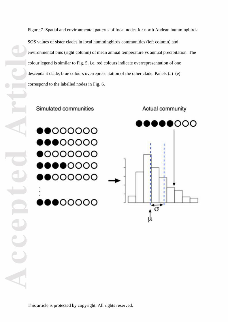
Figure 1. Calculating the SOS value for one community. The example shows the calculation

of specific overrepresentation scores (SOS) for a clade with eight species in the focal

community. The two descendant clades have three (shown as white dots) and five species

(shown as black dots) in the community. A number of random communities are simulated,

creating a distribution of richness values for each descendant clade. From this distribution,

two metrics are identified: r, which is the rank of the empirical community in the distribution;

and SOS, which is the distance between the empirical richness of a descendant and the

simulated mean richness in units of standard deviations.

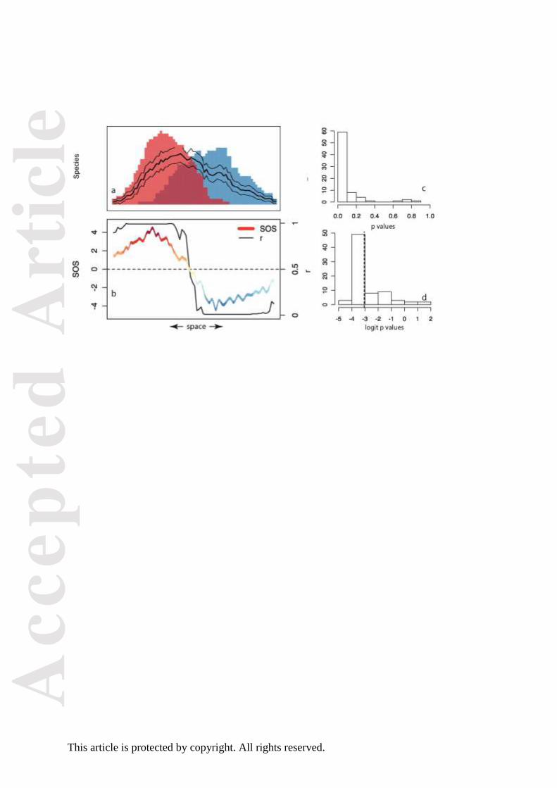
Figure 2. Calculating the GND score from multiple communities. (a) The species richness of

two hypothetical sister clades, marked in blue and red; the expected species richness of each

clade (+- SD) is shown as lines; (b) the value of SOS and r derived from the scenario shown

in panel (a); (c) the distribution of p values, derived from the values of r; (d) the distribution

of p values after logit transformation: the mean value α (-3.05) is shown, corresponding to a

geographic node divergence (GND) value of 0.951 for this clade. The colours of the SOS line

in panel (b) is identical to the colour scheme used in Figs 5 and 7.

Acc

epte

d A

rtic

le


Figure 3. GND values from simulated clades. The lines show the mean of 200 simulations at

each combination of parameter values, and the shaded area indicates the standard deviation.

The horizontal dashed line shows the suggested cut-off of GND = 0.65 for identifying clades

with little distributional overlap. The dots show individual sample runs using the more

computationally intensive 'quasiswap' algorithm.

Figure 4. GND scores of New World flycatchers. The colour scale and symbol sizes are

proportional to GND for each node, to highlight nodes with high GND values. Only fully

resolved nodes where both descendant clades consist of at least two species are included in

the analysis. Nodes labelled A-F are referenced in the text, and correspond to panels (a)–(f) in

Fig. 5. Branch lengths are calculated for illustration using Grafen’s (1989) method– the

analysis itself does not rely on branch lengths. Many genera are unresolved, and appear as

polytomies on the phylogeny.

Figure 5. Spatial pattern of SOS values for six interesting nodes in the phylogeny of New

World flycatchers, in 1° x 1° grid cells. Red colours indicate overrepresentation of one

descendant clade; blue colours indicate overrepresentation of the other descendant clade; and

pale yellow colours indicate that both descendants are equally represented. Panels (a)–(f)

correspond to the labelled nodes in Fig. 4.

Figure 6. GND scores for north Andean hummingbird communities, based on the

geographical (a) and the environmental (b) analysis. The legend is similar to Fig. 4.

Acc

epte

d A

rtic

le


Figure 7. Spatial and environmental patterns of focal nodes for north Andean hummingbirds.

SOS values of sister clades in local hummingbirds communities (left column) and

environmental bins (right column) of mean annual temperature vs annual precipitation. The

colour legend is similar to Fig. 5, i.e. red colours indicate overrepresentation of one

descendant clade, blue colours overrepresentation of the other clade. Panels (a)–(e)

correspond to the labelled nodes in Fig. 6.

Acc

epte

d A

rtic

le


Node-based analysis of species distributions

Documents

Transcript of Node-based analysis of species distributions