WORKING PAPERS IN ECONOMICS

No.07/12

ESPEN BRATBERG, ØIVIND ANTI NILSEN AND KJELL VAAGE IS RECIPIENCY OF DISABILITY PENSION HEREDITARY?

Department of Economics U N I V E R S I T Y OF B E R G EN

Is Recipiency of Disability Pension

Hereditary?*

Espen Bratberg (University of Bergen)

Øivind Anti Nilsen

(Norwegian School of Economics, and IZA-Bonn)

Kjell Vaage (University of Bergen)

April 2012 Abstract

This paper addresses whether children’s exposure to parents receiving disability

benefits induces a higher probability of receiving such benefits themselves. Most

OECD countries experience an increasing proportion of the working-age population

receiving permanent disability benefits. Using data from Norway, a country where

around 10% of the working-age population rely on disability benefits, we find that the

amount of time that children are exposed to their fathers receiving disability benefits

affects their own likelihood of receiving benefits positively. This finding is robust to a

range of different specifications, including family fixed effects.

Keywords: disability, intergenerational correlations, siblings fixed effects JEL classification: H55, J62

* Acknowledgments: This paper has benefitted from comments and suggestions at presentations at 7th Norwegian–German CESifo Seminar, the Norwegian University of Science and Technology, and The Danish National Centre for Social Research (SFI). Department of Economics, University of Bergen, N-5007 Bergen, Norway. E-mail address: espen.bratberg@econ.uib.no Department of Economics, Norwegian School of Economics, N-5045 Bergen, Norway. E-mail address: oivind.nilsen@nhh.no Department of Economics, University of Bergen, N-5007 Bergen, Norway. E-mail address: kjell.vaage@econ.uib.no

1

1. Introduction

In the US and most of Western Europe, the share of the working-age population living

on a disability pension (DP) is increasing (OECD 2010a, Autor and Duggan 2003,

2006). Together with an aging population, this is an increasingly important policy

issue. Several aspects make this a concern. The rising number of disability pensioners

itself puts a strain on public finances. Moreover, reduced fertility rates and increasing

longevity combined with low average retirement ages adds to a worsened dependency

ratio. Put together, these are factors that question the sustainability of the existing

welfare states. To the extent that some people on disability benefits could have been

working, there may also be individual costs in terms of foregone earnings and social

exclusion that result from being outside the labor force.

The increasing DP trend is not reflected in deterioration in general health. On

the contrary, standard health indicators suggest improved public health.1 The

combination of improved public health and rising disability rolls is encountered in

many Western countries; see Autor (2011) for a recent discussion of the US case. This

observation has lead researchers to test other mechanisms and routes to DPs. One

obvious candidate stems from the innate moral hazard problems enforced by the

generosity of the disability insurance systems. In the US, there is a long series of

contributions discussing the incentives produced by US disability programs, such as

Parsons (1980), Leonard (1986), Bound (1989), Chen and van der Klaauw (2008) and

Autor (2011). Börsch-Supan (2007) compares the EU15 countries plus the US, and

finds, after controlling for demographic structure and health status, a substantial cross-

national variation in DP enrolment rates. As much as three quarters of the variation, he

1 See for instance OECD (2010b).

2

claims, is due to country-specific disability insurance rules. Furthermore, Bratsberg et

al. (2010) show that a large percentage of disability insurance claims can be directly

attributed to job displacement and other adverse shocks to employment opportunities

and therefore conclude that unemployment and disability insurance are close

substitutes, at least in Norway. Rege et al. (2007) report substantial social interaction

effects in DP participation among older workers after plant downsizing. Hence, DP, in

addition to being a social insurance against severe health losses, also appears to be

influenced by the labor market and social norms. Norms are established at home and

transferred from parents to children. Our intension in this paper is to disentangle the

different ways through which parental disability is transferred to the next generation.

Parents’ influence on children’s outcome has been studied within many

different fields and from many different angles. As one would expect, economists have

been focused on the transmission of economic status from one generation to the next.

In particular, there is a vast literature on income mobility across generations, expressed

by the estimation of intergenerational earnings elasticities; see Solon (1999) and Black

and Devereux (2011) for overviews and Bratberg et al. (2005), Bratsberg et al. (2007),

and Nilsen et al. (2012) for Norwegian assessments. In later years, however, we have

witnessed a growing interest in other aspects of intergenerational transmission.

Examples, surveyed in Black and Devereux (2011), are education, health, welfare

participation, jobs and occupation, consumption, attitudes, etc. Moreover, it has

become increasingly common to address the causal mechanisms underlying the

intergenerational correlations.

As for DP, Kristensen et al. (2004) report a relatively strong positive

association across generations. Note however, this association is to be interpreted as a

causal link only if the child becomes a DP receiver because of his/her parents

3

receiving the same pension. This is a point that is made in several earlier papers, most

of them based on analysis of intergenerational transmission of welfare benefits and/or

welfare participation; see Duncan et al. (1988), Gottschalk (1990), Levine and

Zimmerman (1996), Pepper (2000), Page and Stevens (2002), and Mitnik (2010) for

US and Canadian analysis.2 Stenberg (2000), Edmark and Hanspers (2011), and

Lorentzen (2010) are recent analysis from Sweden and Norway, respectively. The

Scandinavian welfare model differs somewhat from the other Western economies,

notably the Anglo–American, in its relatively extensive use of unitarian, health-related

social insurance, e.g., DP, at the expense of means-tested welfare benefits. Contrary to

welfare benefits, DP is an absorbing state, meaning that once an individual enters this

form of benefit scheme, he/she rarely returns to self-support. In an ideal world with

perfect information, DP simply serves as insurance against health-related loss of the

ability to work. In reality, however, DP may be used as an early retirement route even

if ability to work has not changed.

There is obvious scope for parents to affect children’s propensity to become

disability benefit receivers. Children inherit their parents’ propensity to become

welfare receivers (partly) as a result of negative impacts from the welfare system. Such

adverse influences can be the result of values, attitudes, and behaviors of parents and

neighbors and/or a decrease in the stigma associated with the welfare system. It may

also be because of the development of self-defeating work attitudes and poor work

ethics.

On the other hand, a positive association might also reflect (observed and

unobserved) characteristics of the family that might have been present before the

parent became a DP receiver. In that case, the observed relationship between the DP

2 For an overview of the sociological literature, see for instance Corcoran (1995)

4

behavior of parents and children could turn out to be spurious. For example,

individuals at the lower end of the earnings distribution are far more likely to end up as

DP receivers than those at the upper end. The income of a pension receiver is further

reduced compared with the earnings before receiving DP. As in Levine and

Zimmerman (1996), the correlation between DP status and their status as low-income

earners makes it difficult to separate the intergenerational transmission of DP from the

intergenerational transmission of earnings.3 If disabled parents provide limited

educational opportunities, live in substandard neighborhoods, etc., it may affect the

children’s education, their probability of living in the same neighborhood, receiving

social insurance and, ultimately, the probability of ending up on public benefits. In

such cases, we will observe a strong correlation between parents’ and children’s DP,

but it will be misleading to argue that parents’ DP is causing the children’s receipt of a

pension. An even more obvious example is health. Poor health is a necessary

qualification for the eligibility of DP. At the same time, it is often the case that children

inherit poor health from their parents. Hence, health is clearly a potential confounding

factor in our attempt to isolate the causal mechanisms behind receiving DP.

In this paper we investigate whether children’s probability of becoming DP

receivers increases the longer they are exposed to parents whom themselves receive

DP. This has the potential of taking our understanding one step further regarding the

way DP is transmitted between generations: genetic susceptibility is congenital and

will not be altered, while children are more likely to pick up their parents’ attitudes and

behavior the longer the duration of exposure. In the analysis we consider the

probability of DP for the offspring before the age of 40; hence, we do not restrict the

3 The authors study mother–daughter correlation for the receipt of American Aid to Families with Dependent Children (AFDC). In terms of Levine and Zimmerman (1996), “the poverty trap will confound the estimation of the welfare trap” (p.3).

5

transmission to take place while the children are living with their parents.4,5 The

analyses are performed on a sample of Norwegian siblings. The ability to identify

siblings is an important characteristic of our data, allowing us to control for fixed,

unobserved heterogeneity within families. To illustrate the advantage of a family fixed-

effect, it may be informative to consider specific sources of parents’ state of disability,

e.g. addiction. According to medical research addiction is to some degree hereditary

(Kendler et al., 2007). Moreover, being exposed to parents being DP receivers because

of, for example, alcohol addiction obviously has adverse effects on children in the

family; increasing, in turn, their own likelihood of becoming DP receivers. The focus

of this paper is the latter effect controlling for the former, which is exactly the virtue of

the family fixed-effect model. Genetic susceptibility is common for the siblings in a

given family and, hence, is integrated out in the fixed-effect model, while the exposure

varies according to the ages during which the siblings were confronted with their

parents’ addiction and DP status.6

By focusing on Norway, we have access to data that enables us to calculate

parent–child correlation but also, more importantly, to explore the mechanisms

underlying the intergenerational correlations in DP receipts. Norway has also

experienced rising rates of DP payments for several decades, and currently has one of

the world’s highest disability rates at 9.5% of the population aged 18–67, according to

the National Insurance Administration (persons on temporary disability benefits not 4 It is possible that the younger children move out relatively earlier as a response to the DP state of their parents (this information is not available in our data). In that case, it may be argued that our measure of exposure will be underestimated for the youngest siblings. 5 In the remainder of this paper we will use the terms child and offspring interchangeably independent of the age of the child/offspring. 6 To the degree that the parents’ receipt of DP is an indicator of poor health, their health condition might influence their opportunities and abilities to take care of their children. If so, this is a case where parents’ poor health affects the children adversely and ultimately might influence their probability of becoming DP receivers. Furthermore, one must assume that this effect increases with duration of exposure.

6

included). No corresponding deterioration in general health has been documented. On

the contrary, standard health indicators, objective as well as subjective, point in the

direction of improved public health (see for instance Norwegian Institute of Public

Health). The Norwegian data have several advantages. First, they are full population

registry data with information on receivers as well as nonreceivers of social insurance

benefits, and the representativeness of the sample is not an issue. Second, we have

longitudinal information on social insurance, making it possible to infer the age of the

offspring when a parent started receiving DP. Thus, we are able to construct a variable

that measures children’s exposure time to parents’ receipt of DP. Third, because our

data include siblings, we can control for unobserved family effects. Finally, with data

on both parents, we are able to analyze differences in the correlations between son–

father, son–mother, daughter–father, and daughter–mother.

Our analysis shows that there is a positive correlation in the probability of

receiving disability benefits between children and parents. We also find that the

amount of time a child is exposed to parents’ receipt of DP benefits affects children’s

likelihood of receiving disability benefits. Finally, when separating the

intergenerational transmission of DP from the transmission of family fixed effects, the

negative and statistically significant effects of exposure to parents’ disability benefits is

still present. Several robustness checks are performed. First, one-child families are

added to the sibling sample. Second, different age group variables are employed to

measure the duration of exposure. Third, “stable” families are estimated separately.

None of the robustness checks reject our main finding; the longer children are exposed

to parents’ receipt of disability benefits the higher their own likelihood of receiving

disability benefits.

7

The rest of the paper is organized as follows. In Section 2 we describe the

institutional background. Our data are presented in Section 3, while the empirical

model is discussed in Section 4. Our results are discussed in Section 5, while some

concluding remarks are given in Section 6.

2. Background and Institutional Details

The Norwegian Act of Disability was passed by the Parliament in 1960. In 1967 it was

integrated with a comprehensive social insurance scheme called The National

Insurance Scheme (NIS). The NIS encompasses the old age retirement scheme,

sickness benefits, disability benefits, unemployment insurance, and health insurance. In

principle the NIS gives full population coverage, with defined benefits based on

earnings histories.

All employees who have been with the same employer for at least four weeks

are covered by the mandatory sickness insurance scheme, which stands out as very

generous compared with other countries. Sickness benefits are paid by the employer

for the first two weeks, and then by the NIS for a maximum of 50 weeks. Individuals

with permanent impairments may apply for disability benefits, roughly corresponding

to old-age pensions. The application must be certified by a physician. Furthermore, the

NIS supplies benefits for participants in medical and vocational rehabilitation. Old-age

pension is a mandatory defined-benefit system, which includes an earnings-based

supplementary benefit in addition to a fixed minimum pension benefit. Disability

benefits are, roughly speaking, calculated as the old-age benefits the beneficiary would

have been entitled to had he/she continued working until the age of 67, the ordinary

retirement age. The average DP compensation ratio is 50–60%. To be eligible for

8

disability benefits, relevant rehabilitation should have been attempted. Rehabilitation

benefits are roughly the same as disability benefits.

The sickness and disability insurance schemes both place heavy burdens on

the Norwegian welfare state. Direct expenditures associated with the sick leave scheme

are in the order of 2.5% of GDP and workdays lost constitute 6.5% of total working

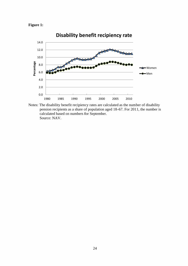
hours. The disability benefit recipiency rate, i.e. the number of DP recipients as a share

of population aged 18–67, is very high in Norway compared with other OECD

countries. Numbers reported by OECD (see OECD 2010a, Figure 2.9), state that in

2008 the recipiency rate was a little higher than 10% in Norway, while the

corresponding number for the OECD on average was just below 6%. The evolution

over time is shown in Figure 1, covering the period 1980–2011. The stock of disability

pensioners rose steadily through the 1970s and 1980s, stabilized in the early 1990s

following a stricter admission policy, increased again from the mid-1990s, and has

decreased somewhat from the turn of the century. As of late 2011, 9.5% of the

population aged 18–67 are disability pensioners. In 2004 a reform introduced

temporary disability benefits that could be granted for a maximum of four years. In

2010, the temporary disability benefits were abolished and replaced with a new

temporary benefits program that also includes previous rehabilitation benefits.

[Figure 1: Evolvement of the disability benefit recipiency rate in Norway]

[Figure 2: The disability benefit recipiency rate by age and sex]

Figure 2 shows that the probability of ending up on disability benefits increases

exponentially with age. As for age 60, we see that approx. 35% of the female

population are receiving disability benefits, while the corresponding numbers for men

9

is 24%. At age 66, one year prior to the standard pension age in Norway, the

corresponding numbers are 49% and 40% (women and men, respectively). This is

shown in Figure 2.

Unlike many other European countries, Norway had no general early

retirement scheme until 1989, when a program was introduced, which covered

employees in the public sector and about half the private sector from the age of 62. The

substitution from disability to this scheme was moderate (Bratberg et al. 2004). In

2011 a major reform of the pension system was introduced, where flexible retirement

from the age of 62 is an integral part. This reform does not affect our analysis, which

covers DPs granted up to the 2004 reform.

3. Data and Sample

We use data from Norwegian registers covering the entire population, provided by

Statistics Norway. Importantly, the data include parent–child links via personal

identifiers. The database includes earnings data starting in 1967 and other background

information with yearly updates from 1986. We also have longitudinal data from the

Norwegian Labour and Welfare Administration (NAV) including information on DP

receipts. The NAV data include two variables that are relevant for determining when a

person started receiving DP: the first date for actual receipt of DP, and the date when

the sickness spell leading to DP started, typically several years before receipt (but the

individual benefits from other social insurance benefits in the meantime). The DP-start

variable is censored in 1991, but not the other variable, which covers spells back to

1966. In the analysis, we base the outcome of children on actual DP starts (the

10

censored variable) while we use the other variable to assess the DP status of parents.7

The NAV data are limited to individuals below the retirement age (67) in 1991, thus

we do not include parents born before 1925.

In the analysis we consider the probability of DP for the child before the age of

40, using the cohorts born 1951–1963, with DP status measured in 1991–2003. The

1963/2003 restriction is because of the reform in 2004 that introduced temporary

disability benefits, see the previous section. This reform implied that some individuals

who would have been granted permanent DP in the old regime were now granted

temporary benefits, but also some who were accepted into the new program might have

been rejected permanent benefits. As we want to focus on the time children are

exposed to parents’ disability, we exclude observations for children whose father

received disability benefits starting before the child was born. This gives us a sample

of 334,995 father–child and 374,307 mother–child pairs. As we shall discuss in the

next section, the main analyses are performed on a sample of siblings, i.e., single

children are excluded. The siblings sample includes 257,705 and 289,032 father–child

and mother–child pairs, respectively. Results using the full sample are reported in the

appendix. To define the outcome variable (DP before the age of 40) we chose the year

of entrance into the absorbing state of permanent DP. This is also consistent with how

disability rates are reported in public statistics. For parents, it is reasonable to assume

that a potential effect on children begins before DP is actually granted, thus the

available variable is well suited for the purpose. The main explanatory variables are

indicators for parental DP receipts, and an interaction term between this indicator and

dummies for offspring age intervals at the beginning of the parental sickness spell

7 The time span between the initial sickness spell and actual DP start varies greatly, with an average of about 4.5 years and a standard deviation of the same magnitude for 35–39 year olds.

11

leading to DP. We control for child and parental cohorts, birth order, parental

education, parents’ age at childbirth, and family income (average for offspring age 16–

19 in 10,000 1989 NOK).

[Table 1 about here]

Table 1 shows the descriptive statistics for the siblings sample that is used in

the main analysis. We note that 4% of male offspring and 5% of female offspring are

DP receivers at age 40, while 44% of fathers and 45% of mothers become DP receivers

during the observation period, indicating that despite the necessity of a medical

diagnosis, DP to some extent may work as an early retirement. We also note that on

average fathers are born in 1930 and mothers in 1933, and were respectively 28 and 25

years old when the children in the sample were born. Mothers on average are

significantly less educated than fathers, reflecting the fact that they grew up in the

1930s and 1940s before the educational explosion.

[Table 2 about here]

Table 2 shows family characteristics by fathers’ disability status, where DP = 1

indicates that the father became a disability recipient before the son/daughter was 40.

We note that the groups are quite similar with regard to cohort and age at childbirth,

but parents in the DP group are less educated. This latter group also has lower incomes,

but as incomes are not necessarily measured before DP was granted, the difference is

not only due to lower labor market earnings. The DP families are slightly larger,

indicated by three or more children.

12

4. Econometric Model

A simple linear probability model for intergenerational correlation in DP, dp, is

(1) ,

where 1(.) is the indicator operator, subscripts ij denote individual i from family j, and

the superscripts c and p denote child and parent, respectively. For sons and daughters,

dp is measured at age 40, for parents, dpjp = 1 indicates disability before the offspring

is 40. Xij is a vector of family (parent and child) characteristics, fj is family-specific

unobservables that may affect the outcome, and uij is a random error term. If there is a

correlation in the probability of DP between the generations, we expect > 0.

If fj is correlated to dpjp, will be biased by unobserved characteristics present

in the family before the father became a DP recipient. Typically, this would be

hereditary factors that affect health, or differences in family preferences. If we have

several observations on each family (i.e. a couple of siblings), the model could be

purged of fj by treating it as an unobserved family fixed effect.8 Note however, the way

equation (1) specifies no variation in dpjp in family j. On the other hand, if there is a

learning effect in the intergenerational transfer of disability, we would expect the

child’s disability probability to be increasing in the time he/she is exposed to parental

disability. Exposure time will vary between siblings, thus a siblings fixed-effect

estimator becomes available by interacting dpjp with exposure. To implement this, we

let aijc denote the age of the child when the parent became disabled and augment (1) to

8 Ekhaugen (2009) exploits sibling variation in a recent paper on intergenerational correlation in unemployment.

ijjijpj

cij ufXdpdpP )1(1)1(

13

(2) ,

where a1 < a2 etc. If exposure time matters, we expect 1 > 2 > 3 > 4. In the main

analysis we use age intervals 1–15, 16–20, 21–30, and 31–40. The first disability spells

in the data start in 1966 when the 1951 (child) cohort was aged 15, hence the upper

limit in the first age interval. The next age interval, 16–20, covers the period before

most children started to study, and therefore, moved out of their parents’ home. In the

appendix we also report results for the cohorts 1957–1963 with 1–10 and 11–20 as the

first age intervals.9 The vector of explanatory variables, Xij includes child and parental

cohort dummies, birth order dummies, father’s and mother’s education and age at

childbirth, and family income. By controlling for cohorts, we avoid time trends in

disability rates leading to spurious results. We estimate (2) by OLS and with siblings

fixed effect. It is worth pointing out that with the siblings fixed effect, one is utilizing

variation in the data within each family. All the variation between families is “swept

out” by the fixed effects. Thus it is likely that the statistical significance decreases.

Finally, earlier research on birth order effects, see for instance Black et al. (2005), and

Lindahl (2008) lead us to expect that younger siblings have a disadvantage. Thus,

controlling for birth order may also be crucial.

9 Alternatively to equation (2), exposure could have been modeled linearly as 1(dpj

p=1)*aijc.

The dummy formulation was chosen because aijc is censored from below, at age 3 for the 1963

cohort, up to age 15 for the 1951 cohort.

ijjijcij

pj

cij

pj

cij

pj

cij

pj

cij

ufXdp

dp

dp

dpdpP

)(1)1(1

)(1)1(1

)(1)1(1

)(1)1(1)1(

544

433

322

211

14

5. Results

Table 3 presents the effect of fathers’ DP on their children’s probability of becoming

disability receivers. In the upper block, sons and daughters are pooled, whereafter they

are estimated separately (mid and lower blocks).

[Table 3 about here]

Column (1) presents the OLS results, with no controls. As expected, there

exists a strong and highly significant effect. From the descriptive statistics in Table 1

we see that 4% of the children in our sample become disability receivers before they

turn 40 (3% of the sons and 5% of the daughters, respectively). This probability

increases to 4.2% for sons (3% + 1.2%) and to 6.3% for daughters (5% + 1.3%). In

relative terms these increases are quite substantial (29% and 21% for sons and

daughters, respectively).

However, the revealed correlation does not answer the questions we ask in this

paper. First, we want test whether the correlation is related to the time the children are

exposed to their parents being disability receivers. For this we use the constructed

indicators for different periods of the children’s lives: ages 0–15, 16–20, 21–30, and

31–40, respectively. The first indicator covers the period up until high school,10 the

second, the high school period, while the final two represents periods of early and mid-

adult life. In other words, we allow social interaction to play a role between and within

families also after the children (typically) have left home. Column (2) sheds light on

this hypothesis. We find the strongest effect for those children that were exposed early

10 Too small samples prevent us performing more detailed stratifications.

15

in their lives and, hence, experienced disabled parents for the longest time. For

example, children being exposed at the age of 0–15 have a 6.5% higher probability of

becoming DP receivers themselves compared with children of the same age with

nonreceiving parents. The effect decreases monotonically the higher the age group and

the shorter the exposure.

In columns (3) and (4) we control for possible confounding factors, still within

an OLS framework. Recent research indicates that younger siblings are at a

disadvantage with respect to outcome in adult life, notably education (Black et al.

2005). Hence, we control for birth order’s possible association to the receipt of DP

(column (3)). As discussed in the introductory section, we do not want to confound

fathers’ disability with low earnings and low education (controlled for in column (4)).

We see that inclusion of controls have only minor effects on our estimates. The

coefficient decreases somewhat, particularly for the youngest group.11 Turning to the

differences between sons and daughter in blocks two and three, we see the same

pattern as before we divided the effect of fathers’ disability into periods of exposure,

namely a stronger effect on daughters compared with that on sons.

It is reassuring that our estimates of the effect of different degrees of exposure

survive the extension of the analysis to include several individual and parental

characteristics. However, the fundamental question of unobserved heterogeneity must

be addressed before we can claim any causal interpretation of our findings. It might

very well be unobserved characteristics of a certain family, present before as well as

after the father receive DP, that is driving the intergenerational correlation; an obvious

candidate being bad health inherited from parent to child. Therefore, we include family

11 It even becomes negatively significant for the oldest group - a result that vanishes in our preferred model.

16

fixed effects in columns (5) and (6). Hence, we forsake the variation between families

in our sample, and isolate any effect that stems from the variation within families. To

the degree that genes matter in deciding the correlation, e.g. through inherited weak

health, it is integrated out by playing an identical role for all siblings in the respective

family.12 In the pooled sample (upper block) we see that the effect from long exposure

diminishes compared with the OLS results, but that is what one might expect when all

the between family effects are omitted. The significantly positive effect remains,

though, before as well as after controlling for observable confounders.13 The pattern is

more or less the same for sons and daughters, but significant only at the 5% level for

sons in the 16–20 age group. The reduced significance is likely to stem from the small

sample sizes of age groups relative to the pooled sample.

It should be noted that when we apply the siblings fixed effects model, only

siblings who are found in different age intervals contribute to the identification of the

exposure variable. There is a trade-off between having more detailed age intervals, and

the number of variables to be identified. In Table A1 we report how many of the

observations actually contribute to the identification. We see that the variation is

smallest in the 0–15 interval, thus there is little scope for finer intervals for those who

were exposed at the youngest age.

[Table 4 about here]

12 As always in fixed-effect models, this rests on the assumption of common trends within each group. 13 The fixed-effect formulation means that only birth order remains relevant, while parental earnings and education become part of the fixed effect.

17

In Table 4, we report a similar intergenerational effect between mothers and

children. The OLS results resemble the ones for fathers. However, when we turn to the

family fixed-effect formulation, the coefficients tend to be smaller in magnitude, and

the effect of having a mother on DP is significant only for the 0–15 age group and at

the 10% level. When we split the sample into sons and daughters, none of the

coefficients are significant at conventional levels. Hence, unobserved family effects

appear to play a more important role for the intergenerational correlation between

mothers and children than for fathers and children.

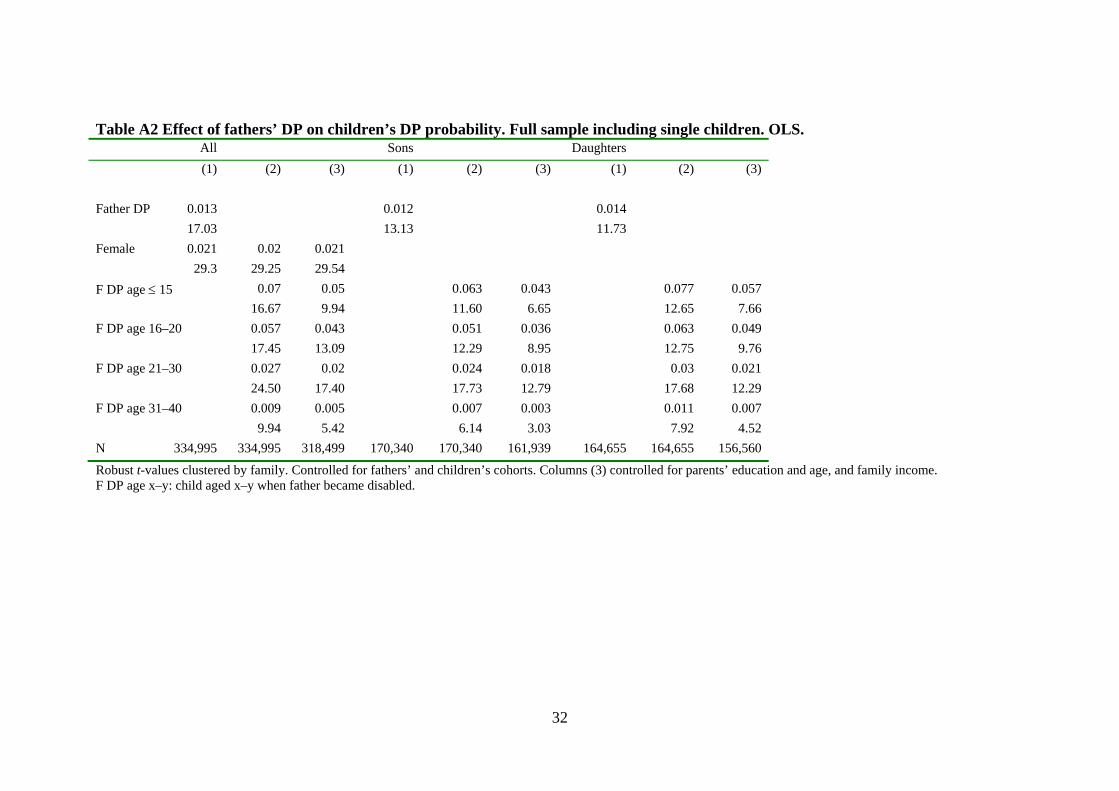
So far the reported regressions were based on a sample of siblings. To check

whether this introduces any selection problems, we run the various OLS regressions for

the full sample including families with only children. The results, reported in Tables

A2 and A3, are quite similar to the OLS results in Tables 3 and 4, implying that biases

due to the selection of families with more than one child is not an issue.

As noted in the data section, the uneven exposure time intervals used in Tables

3 and 4 reflect data limitations with regard to the first disability spells. If we exclude

the 1951–1956 cohorts, we are able to split the exposure dummy at the age of 10 for

the remaining cohorts, 1957–1963. These additional analyses are reported in Tables A4

and A5. The point estimates are quite close to the main results. However, the effect of

fathers’ DP on sons in the first age interval, which was significant in the FE

regressions in Table 3, now turns out to be insignificant, possibly because of the

reduced sample size.

Family dissolutions may affect the outcomes of the children—it is reasonable

that the influence of a parent who moves out could be reduced. Therefore, we have also

estimated the sibling model on a subsample of “stable” families to ensure that the

parents are living together. The data do not include continuous observations on

18

parents’ marital status, but we have census data from 1970 and 1980, and yearly

records from 1987. The 1970 data also include marital duration. Thus we can back-

track marital status from 1980–1987 to childbirth, and define the family as stable if the

parents are married at all observation points.14 In the main analysis, 87.5% of the

sample belongs to stable families according to this definition. Tables A6 and A7 show

the results. In sum, they are quite similar to the main results, but the effect of fathers’

DP on sons does not quite survive in the fixed-effect regressions. Mothers’ DP still has

no effect when controlling for family fixed effects. Taking into account the reduced

sample size and the strict stability definition, we conclude that our main conclusions

are unchanged by this exercise.

6. Concluding remarks

In this paper we address the growing concern caused by rapidly rising disability rolls in

several OECD countries. A particular reason for these concerns is that disability

retirement for all practical purposes is an absorbing state. Thus, the increasing number

of disability pensioners adds to the burden of unfavorable dependence ratios brought

about by demographic changes. We focus on a particular aspect: a possible spillover

effect between generations. Such an alleged spillover represents additional costs that

are likely to be ignored in an analysis based on individuals instead of families. Our

paper attempts to measure empirically to what degree children inherit their parents’

propensity of becoming DP receivers. In doing so, we link the literature on disability

14 The definition of stable depends on the cohort and is stricter for the older cohorts. For the 1951 cohort, our definition implies no parental break-up before offspring are aged 29, age 28 for the 1952 cohort, and so on to age 20 for the 1960 cohort. For the youngest cohorts the age limits are 26, 25, and 24.

19

insurance to the literature on intergenerational transmission of welfare benefits. DP is

social insurance against severe health loss, but the probability of becoming a pension

receiver also appears to be influenced by social norms, partly established in the homes

and distributed from parents to children.

Norway is typical in the sense that the disability rates have increased

dramatically since 1980 while on the other hand, public health has improved; trends

similar to those described by Autor (2011) for the US. Fortunately, Norwegian data are

also exceptionally rich by being based on full population registers, allowing parent–

child links by personal identifiers, and covering a period long enough to address

intergenerational correlations. In addition to having a number of control variables, the

data also allow us to identify siblings. Thus we can consider the importance of

exposure, and apply a family fixed effects model to separate the effect of parental

disability receipts from unobserved family characteristics.

Our OLS results indicate a positive correlation in the probability of receiving

disability benefits between children and parents. The effect is strongest for the children

that experienced disabled parents for the longest time. Turning to the differences

between fathers and mothers and sons and daughters, we observe a slightly stronger

effect on daughters compared with that on sons, no matter which parent receives the

benefit.

In our preferred model we restrict any effect stemming from the variation

within and not between families. This integrates out (time invariant) unobserved family

characteristics and takes us closer to a causal interpretation of our covariations. The

significantly positive effect from father to children remains, before as well as after

controlling for observable confounders, as long as we pool sons and daughters. When

separating sons and daughters and thereby further reducing the sample size, the pattern

20

is more or less the same, but barely significant at the 5% level. The mother–children

effect does not survive the fixed effect model, however.

The existence of a spillover effect between generations implies that DP is not

only a concern for the receiving generation, but also for their children. The apparent

pattern revealed in our paper calls for increased effort in preventing disability

retirement, particularly in families with children that are facing long exposure time. On

the other hand, the same spillover effect represents an extra potential for policies that

manage to lower the DP uptake: the positive effect can be carried on to the next

generation.

21

References

Autor, D. H. (2011) “The unsustainable rise of the disability rolls in the United States:

Causes, consequences, and policy options.” NBER, No. 17697.

Autor, D. H., and M. G. Duggan (2003). “The rise in the disability rolls and the decline

in unemployment.” Quarterly Journal of Economics, 118(1), 157–205.

Autor, D. H., and M. G. Duggan (2006) “The growth in the social security disability

rolls: A fiscal crisis unfolding.” Journal of Economic Perspectives, 20(3), 71–96.

Black, S., P. Devereux and K. Salvanes (2005) “The more the merrier? The effect of

family composition on children’s outcomes”, Quarterly Journal of Economics,

120 (2), 669-700.

Black, S., and P. Devereux (2011) “The recent developments in intergenerational

mobility” (eds. Ashenfelter, O. C., and D. Card), Handbook of Labor Economics,

Vol. 4B, Chapter 16, Elsevier, Amsterdam.

Bound, J. (1989) “The health and earnings of rejected disability insurance applicants.”

American Economic Review, 79(3), 482–503.

Börsch-Supan, A. (2007) “Work disability, health, and incentive effects.” Discussion

Paper No. 07-23, Mannheim: Mannheim Institute for the Economics of Aging,

University of Mannheim, Germany.

Bratberg, E., T. H. Holmås, and Ø. Thøgersen (2004) “Assessing the effects of an early

retirement program.” Journal of Population Economics, 17(3), 387–408.

Bratberg, E., Ø. A. Nilsen, and K. Vaage (2005) “Intergenerational earnings mobility

in Norway: Levels and trends.” Scandinavian Journal of Economics, 107(3),

419–435.

Bratsberg, B., K. Røed, O. Raaum, R. Naylor, M. Jäntti, T. Eriksson, and E.

Österbacka (2007) “Nonlinearities in intergenerational earnings mobility:

Consequences for cross-country comparisons.” Economic Journal, 117(519),

C72–92.

Bratsberg, B., E. Fevang, and K. Røed (2010) “Disability in the welfare state: An

unemployment problem in disguise?” IZA Discussion Paper No. 4897.

Chen, S., and W. van der Klaauw (2008) “The work disincentive effects of the

disability insurance program in the 1990s.” Journal of Econometrics, 142(2),

757–784.

22

Corcoran, M. (1995) “Rags to rags: Poverty and mobility in the United States.” Annual

Review of Sociology, 21, 237–267.

Duncan, G. J., M. S. Hill, and S. D. Hoffman (1988) “Welfare dependence within and

across generations.” Science, 239(4839), 467–471.

Ekhaugen, T. (2009) “Extracting the causal component from the intergenerational

correlation in unemployment.” Journal of Population Economics, 22(1), 97–113.

Edmark, K., and K. Hanspers (2011) “Is welfare dependency inherited? Estimating the

causal welfare transmission effects using Swedish sibling data.” Working paper

2011:25, IFAU, Uppsala.

Gottschalk, P. (1990) “AFDC participation across generations.” The American

Economic Review, 80(2), 367–371

Kendler, K. S., J. Myers, and C. A. Prescott (2007) “Specificity of genetic and

environmental risk factors for symptoms of cannabis, cocaine, alcohol, caffeine,

and nicotine dependence.” Archives of General Psychiatry, 64(11), 1313–1320.

Kristensen, P., T. Bjerkedal, and J. I. Brevik (2004) “Long term effects of parental

disability: A register based life course follow-up of Norwegians born in 1967–

1976” Norsk Epidemiologi, 14(1), 97–105.

Leonard, J. (1986) “Labor supply incentives and disincentives for disabled persons.” In

(ed. Berkowitz, M. and M.A. Hill), Disability and the Labor Market: Economic

problems, policies and programs, Industrial and Economic Relations Press,

Utica, N.Y.

Levine, P. B., and D. J. Zimmerman (1996) “The intergenerational correlation in

AFDC participation: Welfare trap or poverty trap?” Institute for Research on

Poverty, Discussion Paper no. 1100-96.

Lindahl, L. (2008) “Do birth order and family size matter for intergenerational income

mobility?” Applied Economics, 40(17), 2239–2257.

Lorentzen, T. (2010) “Social assistance dynamics in Norway: A sibling study of

intergenerational mobility.” Report 3 – 2010, Stein Rokkan Centre for Social

Studies, Bergen.

Mitnik, O. A. (2010) “Intergenerational transmission of welfare dependency: The

effects of length of exposure.” SOLE Submission.

Nilsen, Ø. A., K. Vaage, A. Aakvik, and K. Å. Jacobsen (2012) “Intergenerational

earnings mobility revisited: Estimates based on lifetime earnings.” Scandinavian

Journal of Economics, 114(1), 1–23.

23

Norwegian Institute of Public Health (2012) “Egenvurdert helse (Self-reported

health).” http://www.fhi.no/artikler/?id=70815, downloaded 2012-02-24.

OECD (2010a) Sickness, Disability and Work: Breaking the Barriers - A synthesis of

findings across OECD countries, OECD Publishing, Paris.

OECD (2010b) Health at a Glance: Europe 2010, OECD Publishing, Paris.

Page, M. E, and A. H. Stevens (2002) “Will you miss me when i am gone? The

economic consequences of absent parents.” NBER Working Paper No. 8786.

Parsons, D. O. (1980) “The decline in male labor force participation.” Journal of

Political Economy, 88(1), 117–134.

Pepper, J. V. (2000) “The intergenerational transmission of welfare receipt: A

nonparametric bounds analysis.” Review of Economics and Statistics, 82(3), 472–

488.

Rege, M, K. Telle, and M. Votruba (2007) “Social interaction effects in disability

pension participation: evidence from plant downsizing.” Research Department,

Statistics Norway, Discussion Papers No. 496.

Solon, G. (1999) “Intergenerational mobility in the labor market.” In (ed. Ashenfelter

O. C., and D. Card), Handbook of Labor Economics, Vol. 3, Part 1, 1761–1800.

Stenberg, S.-Å. (2000) “Inheritance of welfare recipiency: An intergenerational study

of social assistance recipiency in postwar Sweden.” Journal of Marriage and

Family, 62(1), 228–239.

Figu

Not

Percentage

ure 1:

tes: The disapensioncalculatSource:

0.0

2.0

4.0

6.0

8.0

10.0

12.0

14.0

1980

Percentage

ability benen recipients ted based on NAV.

1985

Disab

efit recipiencas a share on numbers f

1990

bility be

24

cy rates areof populatiofor Septemb

1995 200

enefit re

e calculated on aged 18–ber.

00 2005

ecipiency

as the numb67. For 201

2010

y rate

ber of disab11, the numb

Wom

Men

bility ber is

men

25

Figure 2:

Notes: The disability benefit recipiency rates are calculated as the number of disability

pension recipients as a share of population for each age group. Source: NAV.

0.0

5.0

10.0

15.0

20.0

25.0

30.0

35.0

40.0

45.0

50.0

18‐19 20‐24 25‐29 30‐34 35‐39 40‐44 45‐49 50‐54 55‐59 60‐64 65‐67

Percentage

The disability benefit recipiency rate (2009); by age and sex

Men

Women

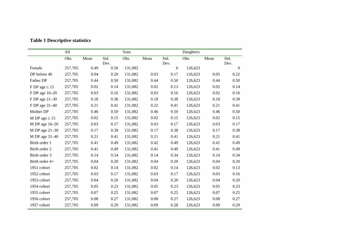
Table 1 Descriptive statistics

All Sons Daughters Obs Mean Std.

Dev. Obs Mean Std.

Dev. Obs Mean Std.

Dev. Female 257,705 0.49 0.50 131,082 0 126,623 0 DP before 40 257,705 0.04 0.20 131,082 0.03 0.17 126,623 0.05 0.22 Father DP 257,705 0.44 0.50 131,082 0.44 0.50 126,623 0.44 0.50 F DP age 15 257,705 0.02 0.14 131,082 0.02 0.13 126,623 0.02 0.14 F DP age 16–20 257,705 0.03 0.16 131,082 0.03 0.16 126,623 0.02 0.16 F DP age 21–30 257,705 0.18 0.38 131,082 0.18 0.38 126,623 0.18 0.39 F DP age 31–40 257,705 0.21 0.41 131,082 0.22 0.41 126,623 0.21 0.41 Mother DP 257,705 0.46 0.50 131,082 0.46 0.50 126,623 0.46 0.50 M DP age 15 257,705 0.02 0.15 131,082 0.02 0.15 126,623 0.02 0.15 M DP age 16–20 257,705 0.03 0.17 131,082 0.03 0.17 126,623 0.03 0.17 M DP age 21–30 257,705 0.17 0.38 131,082 0.17 0.38 126,623 0.17 0.38 M DP age 31–40 257,705 0.21 0.41 131,082 0.21 0.41 126,623 0.21 0.41 Birth order 1 257,705 0.41 0.49 131,082 0.42 0.49 126,623 0.41 0.49 Birth order 2 257,705 0.41 0.49 131,082 0.41 0.49 126,623 0.41 0.49 Birth order 3 257,705 0.14 0.34 131,082 0.14 0.34 126,623 0.14 0.34 Birth order 4+ 257,705 0.04 0.20 131,082 0.04 0.20 126,623 0.04 0.20 1951 cohort 257,705 0.02 0.14 131,082 0.02 0.14 126,623 0.02 0.13 1952 cohort 257,705 0.03 0.17 131,082 0.03 0.17 126,623 0.03 0.16 1953 cohort 257,705 0.04 0.20 131,082 0.04 0.20 126,623 0.04 0.20 1954 cohort 257,705 0.05 0.23 131,082 0.05 0.23 126,623 0.05 0.23 1955 cohort 257,705 0.07 0.25 131,082 0.07 0.25 126,623 0.07 0.25 1956 cohort 257,705 0.08 0.27 131,082 0.08 0.27 126,623 0.08 0.27 1957 cohort 257,705 0.09 0.29 131,082 0.09 0.28 126,623 0.09 0.29

27

1958 cohort 257,705 0.10 0.30 131,082 0.10 0.30 126,623 0.10 0.30 1959 cohort 257,705 0.11 0.31 131,082 0.11 0.31 126,623 0.11 0.31 1960 cohort 257,705 0.11 0.31 131,082 0.11 0.31 126,623 0.11 0.31 1961 cohort 257,705 0.11 0.31 131,082 0.11 0.31 126,623 0.11 0.31 1962 cohort 257,705 0.10 0.30 131,082 0.10 0.30 126,623 0.10 0.30 1963 cohort 257,705 0.10 0.30 131,082 0.10 0.30 126,623 0.10 0.30 Father’s educ. 257,705 11.94 2.68 131,082 11.95 2.73 126,623 11.93 2.62 Mother’s educ. 247,923 8.98 2.10 126,090 8.98 2.10 121,833 8.98 2.09 Father’s age 257,705 27.87 4.00 131,082 27.86 4.00 126,623 27.87 4.00 Mother’s age 249,814 25.19 4.07 127,032 25.18 4.07 122,782 25.20 4.06 Family income 254,929 10.87 4.57 129,696 10.90 4.59 125,233 10.85 4.55 Father’s cohort 257,705 1930.50 3.92 131,082 1930.48 3.92 126,623 1930.53 3.92 Mother’s cohort 249,814 1933.20 4.21 127,032 1933.17 4.22 122,782 1933.22 4.20

Notes: Family income in 10,000 1989 NOK, average for child aged 16–19. F/M DP age x–y: child aged x–y when father/mother became disabled.

Table 2 Family characteristics by fathers’ disability status DP = 0 DP = 1 Obs Mean Std.

Dev. Obs Mean Std.

Dev. All Female 145,050 0.49 0.50 112,655 0.49 0.50 Father’s educ. 145,050 12.24 2.76 112,655 11.56 2.51 Mother’s educ. 139,727 9.26 2.23 108,196 8.62 1.85 Father’s age 145,050 27.90 4.03 112,655 27.82 3.96 Mother’s age 140,835 25.33 4.07 108,979 25.01 4.06 Family income 144,325 11.78 4.68 110,604 9.69 4.14 Father’s cohort 145,050 1930.51 3.90 112,655 1930.49 3.94 Mother’s cohort 140,835 1933.10 4.18 108,979 1933.32 4.24 Birth order 1 145,050 0.43 0.49 112,655 0.40 0.49 Birth order 2 145,050 0.41 0.49 112,655 0.41 0.49 Birth order 3 145,050 0.13 0.33 112,655 0.15 0.35 Birth order 4+ 145,050 0.04 0.19 112,655 0.05 0.22 Sons , Father’s educ. 73,825 12.23 2.84 57,257 11.58 2.52 Mother’s educ. 71,124 9.26 2.23 54,966 8.62 1.86 Father’s age 73,825 27.91 4.02 57,257 27.80 3.97 Mother’s age 71,665 25.33 4.07 55,367 24.99 4.07 Family income 73,436 11.81 4.72 56,260 9.71 4.14 Father’s cohort 73,825 1930.48 3.90 57,257 1930.47 3.94 Mother’s cohort 71,665 1933.08 4.19 55,367 1933.30 4.25 Birth order 1 73,825 0.43 0.49 57,257 0.40 0.49 Birth order 2 73,825 0.41 0.49 57,257 0.40 0.49 Birth order 3 73,825 0.13 0.33 57,257 0.15 0.35 Birth order 4+ 73,825 0.04 0.19 57,257 0.05 0.22 Daughters Father’s educ. 71,225 12.24 2.68 55,398 11.54 2.50 Mother’s educ. 68,603 9.26 2.23 53,230 8.61 1.84 Father’s age 71,225 27.89 4.03 55,398 27.84 3.96 Mother’s age 69,170 25.33 4.07 53,612 25.03 4.04 Family income 70,889 11.74 4.65 54,344 9.67 4.14 Father’s cohort 71,225 1930.55 3.90 55,398 1930.50 3.93 Mother’s cohort 69,170 1933.13 4.18 53,612 1933.33 4.23 Birth order 1 71,225 0.42 0.49 55,398 0.39 0.49 Birth order 2 71,225 0.41 0.49 55,398 0.41 0.49 Birth order 3 71,225 0.13 0.33 55,398 0.15 0.36 Birth order 4+ 71,225 0.04 0.19 55,398 0.05 0.22

29

Table 3 Effect of fathers’ DP on children’s DP probability. OLS and family fixed effects (FE) OLS FE (1) (2) (3) (4) (5) (6) All N = 257,705 Father DP 0.013 14.86 Female 0.020 0.020 0.020 0.020 0.020 0.020 25.49 25.47 25.41 25.35 20.23 20.21 F DP age 15 0.065 0.064 0.043 0.035 0.035 13.9 13.67 7.86 2.80 2.82 F DP age 16–20 0.057 0.056 0.043 0.036 0.036 15.46 15.18 11.68 4.22 4.19 F DP age 21–30 0.025 0.025 0.018 0.022 0.021 20.46 19.84 14.45 3.7.0 3.53 F DP age 31–40 0.008 0.008 0.004 0.014 0.013 8.32 8.00 4.17 2.70 2.43 Sons N = 131,082 Father DP 0.012 11.57 F DP age 15 0.057 0.056 0.035 0.033 0.033 9.55 9.36 5.03 1.21 1.22 F DP age 16–20 0.052 0.051 0.038 0.036 0.036 11.11 10.89 8.23 2.04 2.03 F DP age 21–30 0.023 0.022 0.017 0.024 0.023 15.09 14.6 10.84 1.91 1.84 F DP age 31–40 0.006 0.006 0.003 0.017 0.016 4.92 4.73 2.18 1.54 1.43 Daughters N = 126,623 Father DP 0.013 10.26 F DP age 15 0.074 0.072 0.051 0.038 0.039 10.81 10.64 6.32 1.37 1.39 F DP age 16–20 0.063 0.061 0.049 0.036 0.036 11.17 10.97 8.55 1.90 1.88 F DP age 21–30 0.028 0.027 0.02 0.021 0.02 14.67 14.23 10.1 1.60 1.52 F DP age 31–40 0.011 0.01 0.006 0.012 0.011 6.82 6.56 3.56 1.05 0.92 Controls: Birth order X X X Parents’ education, earnings, age

X

Family fixed effects X X

Robust t-values clustered by family. Controlled for fathers’ and children’s cohorts. F DP age x–y: child aged x–y when father became disabled. Siblings sample, cohorts 1951–1963.

30

Table 4 Effect of mothers’ DP on children’s DP probability. OLS and family fixed effects (FE). OLS FE (1) (2) (3) (4) (5) (6) All N = 289,032 Mother DP 0.011 13.24 Female 0.020 0.020 0.020 0.020 0.020 0.020 26.18 26.16 26.13 25.34 20.84 20.82 M DP age 15 0.057 0.056 0.043 0.018 0.018 15.81 15.59 11.29 1.90 1.86 M DP age 16–20 0.051 0.051 0.041 0.007 0.007 17.6 17.31 12.95 1.11 0.99 M DP age 21–30 0.031 0.031 0.025 0.003 0.001 26.11 25.5 19.63 0.57 0.29 M DP age 31–40 0.011 0.011 0.009 0.001 0.000 11.86 11.54 8.82 0.31 –0.09 Sons N = 146,976 Mother DP 0.008 8.44 M DP age 15 0.049 0.048 0.032 0.014 0.014 10.86 10.70 7.10 0.67 0.67 M DP age 16–20 0.041 0.04 0.028 0.006 0.006 11.22 10.99 7.48 0.44 0.39 M DP age 21–30 0.023 0.023 0.019 0.004 0.003 16.10 15.67 12.03 0.42 0.28 M DP age 31–40 0.009 0.009 0.007 0.002 0.001 7.80 7.62 6.03 0.33 0.12 Daughters N = 142,056 Mother DP 0.013 10.62 M DP age 15 0.065 0.064 0.054 0.022 0.022 12.24 12.07 9.16 1.03 1.00 M DP age 16–20 0.063 0.062 0.054 0.008 0.007 13.93 13.73 10.80 0.54 0.48 M DP age 21–30 0.039 0.039 0.032 0.001 0.00 21.21 20.74 15.86 0.08 –0.04 M DP age 31–40 0.014 0.013 0.01 –0.001 –0.002 9.11 8.86 6.56 –0.07 –0.24 Controls: Birth order X X X Parents’ education, earnings, age X Family fixed effects X X

Robust t-values clustered by family. Controlled for fathers’ and children’s cohorts. F DP age x–y: child aged x–y when father became disabled. Siblings sample, cohorts 1951–1963.

APPENDIX Table A1 Within family variation in exposure to father’s or mother’s DP. Father DP Mother DP

Child age when parent becomes DP

Same Other Total Same Other Total Total

Never 142,108 2,408 144,516 154,315 6,024 160,339 160,339 1–15 3,050 1,829 4,879 4,504 2,602 7,106 7,106

16–20 1,652 4,793 6,445 2,664 7,040 9,704 9,704 21–30 23,750 22,722 46,472 28,051 23,647 51,698 51,698 31–40 32,688 22,705 55,393 35,347 24,838 60,185 60,185

Total 203,248 54,457 257,705 224,881 64,151 289,032 289,032

Same: exposed at same age as siblings. Other: exposed at different age from siblings (at least one sibling).

32

Table A2 Effect of fathers’ DP on children’s DP probability. Full sample including single children. OLS. All Sons Daughters (1) (2) (3) (1) (2) (3) (1) (2) (3) Father DP 0.013 0.012 0.014 17.03 13.13 11.73 Female 0.021 0.02 0.021 29.3 29.25 29.54 F DP age 15 0.07 0.05 0.063 0.043 0.077 0.057 16.67 9.94 11.60 6.65 12.65 7.66 F DP age 16–20 0.057 0.043 0.051 0.036 0.063 0.049 17.45 13.09 12.29 8.95 12.75 9.76 F DP age 21–30 0.027 0.02 0.024 0.018 0.03 0.021 24.50 17.40 17.73 12.79 17.68 12.29 F DP age 31–40 0.009 0.005 0.007 0.003 0.011 0.007 9.94 5.42 6.14 3.03 7.92 4.52 N 334,995 334,995 318,499 170,340 170,340 161,939 164,655 164,655 156,560

Robust t-values clustered by family. Controlled for fathers’ and children’s cohorts. Columns (3) controlled for parents’ education and age, and family income. F DP age x–y: child aged x–y when father became disabled.

33

Table A3 Effect of mothers’ DP on children’s DP probability. Full sample including single children. OLS. All Sons Daughters (1) (2) (3) (1) (2) (3) (1) (2) (3) Mother DP

0.01 0.007 0.012

13.47 8.09 11.1 Female 0.02 0.02 0.021 30.45 30.44 29.55 M DP age 15 0.059 0.047 0.05 0.035 0.068 0.058 19.03 13.95 12.7 8.71 14.84 11.2M DP age 16–20 0.053 0.042 0.039 0.027 0.067 0.058 20.63 15.24 12.48 8.24 16.76 13.06M DP age 21–30 0.032 0.026 0.024 0.019 0.04 0.033 30.2 23.09 18.34 14.18 24.6 18.51M DP age 31–40 0.012 0.009 0.008 0.007 0.015 0.012 13.89 10.43 8.04 6.19 11.53 8.48N 374,307 374,307 318,486 190,301 190,301 161,933 184,006 184,006 156,553Robust t-values clustered by family. Controlled for mothers’ and children’s cohorts. Columns (3) controlled for parents’ education and age, and family income. M DP age x–y: child aged x–y when mother became disabled.

Table A4 Effect of fathers’ DP on children’s DP probability. OLS and family fixed effects (FE). Cohorts 1957–1963. OLS FE (1) (2) (3) (4) (5) (6) All N = 183,345 Father DP 0.012 12.09 Female 0.02 0.02 0.02 0.02 0.02 0.02 21.44 21.48 21.43 22.31 14.91 14.9 F DP age 10 0.062 0.061 0.039 0.022 0.022 8.16 8.01 4.05 0.94 0.96 F DP age 11–20 0.058 0.057 0.042 0.034 0.034 16.78 16.48 11.59 2.53 2.49 F DP age 21–30 0.024 0.023 0.017 0.025 0.023 17.53 16.96 12.13 2.34 2.22 F DP age 31–40 0.007 0.007 0.003 0.02 0.018 5.70 5.39 2.35 2.05 1.88 Sons N = 92,829 Father DP 0.012 9.38 F DP age 10 0.054 0.053 0.033 0.021 0.021 5.61 5.48 2.72 0.38 0.39 F DP age 11–20 0.051 0.05 0.035 0.037 0.037 11.63 11.38 7.82 1.09 1.08 F DP age 21–30 0.022 0.021 0.016 0.026 0.025 12.94 12.48 9.17 0.99 0.94 F DP age 31–40 0.005 0.004 0.001 0.023 0.021 2.93 2.72 0.77 0.92 0.86 Daughters N = 90,516 Father DP 0.013 8.24 F DP age 10 0.07 0.069 0.045 0.022 0.023 6.14 6.05 3.08 0.36 0.37 F DP age 11–20 0.066 0.065 0.049 0.032 0.031 12.5 12.3 8.77 0.91 0.89 F DP age 21–30 0.026 0.025 0.018 0.024 0.022 12.39 12.03 8.34 0.89 0.83 F DP age 31–40 0.01 0.01 0.005 0.018 0.016 5.01 4.78 2.38 0.73 0.65 Controls: Birth order X X X Parents’ education, earnings, age

X

Family fixed effects X X

Robust t-values clustered by family. Controlled for fathers’ and children’s cohorts. F DP age x–y: child aged x–y when father became disabled. Siblings sample, cohorts 1957–1963.

35

Table A5 Effect of mothers’ DP on children’s DP probability. OLS and family fixed effects (FE). Cohorts 1957–1963. OLS FE (1) (2) (3) (4) (5) (6) All N = 200,963 Mother DP 0.011 11.61 Female 0.02 0.02 0.02 0.021 0.02 0.02 21.63 21.62 21.59 22.26 15.03 15.01 M DP age 10 0.057 0.056 0.043 0.021 0.021 9.85 9.71 6.97 1.00 1.00 M DP age 11–20 0.054 0.053 0.042 0.003 0.002 19.1 18.75 13.92 0.3 0.23 M DP age 21–30 0.031 0.03 0.025 0.005 0.004 22.63 22.00 17.10 0.71 0.55 M DP age 31–40 0.011 0.011 0.009 0.004 0.002 9.3 9.01 6.88 0.66 0.42 Sons N = 101,669 Mother DP 0.009 7.87 M DP age 10 0.057 0.056 0.041 0.014 0.014 7.38 7.28 5.07 0.24 0.24 M DP age 11–20 0.043 0.042 0.029 0.000 0.000 12.3 12.04 8.06 0.01 -0.01 M DP age 21–30 0.024 0.023 0.019 0.001 0.000 14.29 13.84 10.94 0.05 -0.02 M DP age 31–40 0.01 0.009 0.007 0.006 0.004 6.33 6.15 4.70 0.40 0.30 Daughters N = 99,294 Mother DP 0.013 8.81 M DP age 10 0.057 0.056 0.045 0.029 0.029 6.81 6.7 4.85 0.56 0.56 M DP age 11–20 0.066 0.065 0.056 0.005 0.004 15.02 14.78 11.58 0.19 0.16 M DP age 21–30 0.038 0.037 0.030 0.008 0.007 17.97 17.51 13.38 0.43 0.37 M DP age 31–40 0.013 0.013 0.010 0.001 0.000 6.95 6.73 5.12 0.09 0.00 Controls: Birth order X X X Parents’ education, earnings, age

X

Family fixed effects X X

Robust t-values clustered by family. Controlled for mothers’ and children’s cohorts. M DP age x–y: child aged x–y when mother became disabled. Siblings sample, cohorts 1957–1963.

36

Table A6 Effect of fathers’ DP on children’s DP probability. Stable families. OLS and family fixed effects (FE). OLS FE (1) (2) (3) (4) (5) (6) All N = Father DP 0.011 13.2 Female 0.020 0.020 0.020 0.020 0.020 0.020 24.58 24.57 24.52 24.38 19.44 19.42 F DP age 15 0.058 0.057 0.041 0.028 0.028 11.28 11.07 6.98 2.05 2.08 F DP age 16–20 0.05 0.049 0.041 0.028 0.028 12.46 12.17 10.16 3.09 3.08 F DP age 21–30 0.024 0.023 0.018 0.02 0.019 18.6 18.02 13.92 3.23 3.08 F DP age 31–40 0.008 0.008 0.005 0.013 0.012 8.20 7.89 4.40 2.43 2.18 Sons N = 114,604 Father DP 0.01 9.65 F DP age 15 0.052 0.05 0.033 0.026 0.027 7.88 7.68 4.47 0.90 0.92 F DP age 16–20 0.045 0.044 0.035 0.032 0.032 9.03 8.78 7.19 1.65 1.65 F DP age 21–30 0.021 0.02 0.016 0.023 0.022 13.06 12.6 9.82 1.71 1.63 F DP age 31–40 0.006 0.006 0.003 0.016 0.015 4.84 4.66 2.07 1.37 1.25 Daughters N = 110,678 Father DP 0.013 9.56 F DP age 15 0.065 0.064 0.049 0.031 0.031 8.7 8.57 5.66 0.97 0.98 F DP age 16–20 0.055 0.054 0.046 0.024 0.023 9.09 8.9 7.51 1.18 1.17 F DP age 21–30 0.028 0.027 0.021 0.018 0.017 13.86 13.46 10.22 1.30 1.23 F DP age 31–40 0.011 0.011 0.007 0.011 0.01 6.7 6.44 3.94 0.90 0.79 Controls: Birth order X X X Parents’ education, earnings, age

X

Family fixed effects X X

Robust t-values clustered by family. Controlled for fathers’ and children’s cohorts. F DP age x–y: child aged x–y when father became disabled. Parents married throughout child’s adolescence.

37

Table A7 Effect of mothers’ DP on children’s DP probability. Stable families. OLS and family fixed effects (FE). OLS FE (1) (2) (3) (4) (5) (6) All N = 234,475 Mother DP 0.009 10.24 Female 0.02 0.02 0.02 0.02 0.02 0.02 24.81 24.78 24.73 24.39 19.83 19.82 M DP age 15 0.047 0.046 0.038 –0.001 –0.001 11.67 11.44 9.29 –0.05 –0.04 M DP age 16–20 0.045 0.044 0.037 –0.003 –0.003 13.1 12.82 10.65 -0.38 –0.44 M DP age 21–30 0.029 0.028 0.023 –0.004 –0.005 21.93 21.33 17.33 –0.83 –1.02 M DP age 31–40 0.011 0.011 0.008 –0.003 –0.004 10.73 10.39 8.17 –0.85 –1.16 Sons N = 119,263 Mother DP 0.006 5.66 M DP age 15 0.036 0.035 0.028 0.002 0.002 7.29 7.12 5.75 0.06 0.06 M DP age 16–20 0.028 0.027 0.021 0.002 0.001 7.22 6.98 5.29 0.09 0.06 M DP age 21–30 0.02 0.019 0.016 0 –0.001 12.99 12.58 10.18 –0.01 –0.09 M DP age 31–40 0.009 0.008 0.007 –0.002 –0.003 6.94 6.75 5.28 –0.43 –0.65 Daughters N = 115,212 Mother DP 0.012 8.82 M DP age 15 0.059 0.058 0.048 –0.003 –0.003 9.47 9.31 7.57 –0.12 –0.12 M DP age 16–20 0.061 0.06 0.053 –0.008 –0.008 11.3 11.12 9.54 –0.48 –0.50 M DP age 21–30 0.037 0.037 0.03 –0.009 –0.009 18.17 17.72 14.35 –0.79 –0.88 M DP age 31–40 0.013 0.013 0.01 –0.005 –0.006 8.33 8.04 6.31 –0.58 –0.74 Controls: Birth order X X X Parents’ education, earnings, age

X

Family fixed effects X X

Robust t-values clustered by family. Controlled for mothers’ and children’s cohorts. M DP age x–y: child aged x–y when mother became disabled. Parents married throughout child’s adolescence.

Department of Economics University of Bergen Fosswinckels gate 14 N-5007 Bergen, Norway Phone: +47 55 58 92 00 Telefax: +47 55 58 92 10 http://www.svf.uib.no/econ