No. 632

Firms, Informality and Development: Theory and

evidence from Brazil

Gabriel Ulyssea

TEXTO PARA DISCUSSÃO

DEPARTAMENTO DE ECONOMIA www.econ.puc-rio.br

Firms, Informality and Development: Theory andevidence from Brazil∗

Gabriel Ulyssea†

PUC-Rio

December 22, 2014

Abstract

This paper develops and estimates an equilibrium model where heterogeneous firmscan exploit two margins of informality: (i) not register their business, the extensivemargin; and (ii) hire workers "off the books", the intensive margin. The modelencompasses the main competing frameworks for understanding informality andprovides a natural setting to infer their empirical relevance. The counterfactualanalysis shows that once the intensive margin is accounted for, aggregate firm andlabor informality need not move in the same direction as a result of policy changes.Lower informality can be, but is not necessarily associated to higher GDP, TFP orwelfare.

JEL Codes: O17, C54, O12.

∗I am indebted to James Heckman, Steven Durlauf and Chang-Tai Hsieh for their guidance andconstant encouragement. I would like to thank Ricardo Paes de Barros, Azeem Shaik, Rafael Lopes deMelo, Gary Becker (in memoriam), Ben Moll, Rodrigo Soares, Carlos Henrique Corseuil, Miguel Foguel,Leandro Carvalho e Silvia H. Barcellos for their comments and helpful discussions. Special thanksto Claudio Ferraz, Rafael Dix-Carneiro, Stephane Wolton and Dimitri Szerman for their detailed andextremely helpful comments and feedback. I am also thankful to seminar participants at the WinterMeeting of the Econometric Society, Yale, Johns Hopkins, Chicago, IDB, Einaudi Institute, EESP-FGV,EPGE-FGV, PUC-Rio, IPEA, and the Annual Meeting of the Brazilian Econometric Society for helpfulcomments and suggestions. Of course, all errors are mine. Financial support from CAPES, IPEA andThe University of Chicago is gratefully acknowledged.†Address: Department of Economics, Pontifícia Universidade Católica do Rio de Janeiro, Rua Mar-

quês de São Vicente, 225, Gávea. Rio de Janeiro, RJ, 22451-900, Brasil. Email: ulyssea@econ.puc-rio.br.

1 Introduction

The informal sector is a prominent feature of most developing economies.1 The highlevels of informality observed in these countries are likely to have deep economic impli-cations. First, they imply widespread tax avoidance, hindering government’s ability toprovide public goods. Second, informality may distort firms’ decisions along importantmargins, such as the size of their labor force.2 Third, it allows less productive (infor-mal) firms to compete with more productive (formal) firms, leading to misallocation ofresources and potentially large TFP losses [e.g. Hsieh and Klenow (2009)]. Oppositely,informality can be beneficial to growth as it provides de facto flexibility for firms thatwould be otherwise constrained by burdensome regulations [Meghir et al. (2014)]. Finally,it has been increasingly emphasized that the informal sector might play an important rolein shaping welfare consequences from trade liberalization in developing countries.3 Thus,understanding how the informal sector affects the economy and evaluating the firm-leveland aggregate impacts of policies towards informality are central issues in economic de-velopment.

To get to these questions, it is crucial to have a clear understanding about the roleof informal firms in the economy. There exist three competing views of what this rolemight be [La Porta and Shleifer (2014)]. The first argues that the informal sector is areservoir of potentially productive entrepreneurs who are kept out of formality by highregulatory costs, most notably entry regulation. The second view sees informal firms as"parasite firms" that are productive enough to survive in the formal sector but choose toremain informal to earn higher profits from the cost advantages of not complying withtaxes and regulations.4 The third argues that informality is a survival strategy for lowskill individuals, who are too unproductive to ever become formal. These views offervery different perspectives on informality and its potential consequences for economicdevelopment. Nevertheless, there is no consensus about their empirical relevance andtherefore about how important they are for understanding informality [Arias et al. (2010)].

In this paper I propose a new framework that distinguishes two margins of informal-ity: (i) whether firms register and pay entry fees to achieve a formal status, the extensive

1In Brazil, nearly two thirds of businesses, 40% of GDP and 35% of employees are informal. Similarly,the informal sector accounts for around 50% of the labor force and 41.9% of GDP in Colombia, and 60%of workers and 31.9% of GDP in Mexico (Figure A.1). For information on informal sector’s size aroundthe world, see Figure A.1, Schneider (2005) and La Porta and Shleifer (2008, 2014).

2For example, if enforcement is tighter for larger firms, there will be incentives to remain small inorder to avoid taxes and regulations.

3See Goldberg and Pavcnik (2003, 2007), Bosch et al. (2012), Menezes-Filho and Muendler (2011),Dix-Carneiro and Kovak (2014) and Cosar et al. (2014).

4The first view dates back to the work of De Soto (1989), while the second view has been put forwardby Farrell (2004) and Levy (2008), among others.

1

margin; and (ii) whether firms that are formal in the first sense hire workers "off thebooks", the intensive margin. The latter is a key innovation, both conceptually andquantitatively. The existing literature has focused on the extensive margin alone, whichimplies that being informal is a binary decision to comply or not with taxes and regula-tions.5 I build on this literature to introduce the intensive margin, which breaks the directassociation between firm and worker informality. Accounting for both margins also allowsto uncover new and subtler firm-level responses to policy changes regarding informalitydecisions. I show that these responses translate into non-obvious and quantitatively im-portant effects on TFP, GDP, and aggregate informality. Empirically, I present evidencethat the intensive margin accounts for a large share of total informal employment.

In the model, sector membership is defined by the extensive margin, and the (in)formalsector is formed by (un)registered firms. If a firm decides to be formal, it faces fixed entry(registration) costs and higher variable costs due to revenue and labor taxes. However,it may avoid the latter by hiring informal workers. If a firm decides to be informalit avoids all taxes and regulations, but faces an expected cost of being caught that isincreasing in firm’s size. Since productivity and size are one-to-one in the model, moreproductive firms (in expectation) self-select into the formal sector and less productivefirms enter the informal sector. Having both margins of informality introduces a size-dependent distortion in the economy that is able to rationalize two prominent features offirm size distribution in developing countries: the absence of meaningful discontinuitiesor bunching of firms at specific points; and the vast predominance of small firms with asmall number of medium sized and large firms, even in the formal sector [Hsieh and Olken(2014)].6 Additionally, the model predicts some overlap between formal and informalproductivity and firm size distributions, as observed in the data.

The proposed model encompasses the three leading views about informal firms dis-cussed above, and is able to integrate them in a unified setting. Even though these viewsare seen as opposing frameworks, I show that in fact they are not. They simply reflectheterogeneous firms choosing whether to comply given the institutional framework theyface. The central distinction lies in their predictions about informal firms’ behavior inface of specific policy changes. I exploit these differences to define a taxonomy of informalfirms based on these views, which provides a natural setting to infer how important theyare in the data.7 I estimate the model with the simulated method of moments and using

5See Rauch (1991), Fortin et al. (1997), Amaral and Quintin (2006), de Paula and Scheinkman (2010,2011), and Galiani and Weinschelbaum (2012), among others.

6For recent studies on the impacts of size-dependent frictions in both developed and developingcountries, see Guner et al. (2008), Garicano et al. (2013) and Adamopoulos and Restuccia (2013).

7The relevant margin to define the taxonomy is the extensive margin. Nevertheless, the intensivemargin is central for measuring correctly the relative size of each view in the data and, most importantly,

2

three different data sources on formal and informal firms and workers in Brazil. I thenuse the estimated model and the proposed taxonomy to infer the relative size of eachview in the data.

The results show that the potentially productive entrepreneurs that are restricted byhigh bureaucratic entry costs correspond to 16.8% of all informal firms. Those that areproductive enough to survive in the formal sector but choose to remain informal to earnhigher profits correspond to 38.7% of informal firms. The remaining firms correspond tothose too unproductive to ever become formal, which are only able to survive becausethey avoid taxes and regulations. These results suggest that informal firms are to a largeextent "parasite firms" and therefore eradicating them (e.g. through tighter enforcement)could produce positive effects on the economy. Oppositely, given the small fraction ofinformal firms constrained by entry costs, reducing these would have limited effects oninformality and overall economic performance.

In order to assess these conjectures, I use the estimated model to conduct counter-factual analyses of different formalization policies. I consider four prototypical policyinterventions: (i) reducing formal sector’s entry costs; (ii) reducing the payroll tax; (iii)increasing the cost of the extensive margin of informality through greater enforcementon informal firms (e.g. more government auditing); and (iv) increasing the costs of theintensive margin through tighter enforcement on formal firms that hire informal workers.

At the firm level, the results show that reducing formal sector’s entry cost has largepositive impacts on informal firms that formalize – an average gain of 24% in terms oftheir own lifetime profits at baseline – but it has negative effects on other firms. Thelatter is a consequence of general equilibrium effects: greater entry increases competi-tion and therefore the equilibrium wage increases, hurting incumbents in both sectors.Increasing the costs of the extensive margin of informality benefits formal incumbents,but particularly so low-productivity formal firms. This result thus indicates that thesefirms are the most directly affected by informal firms’ competition. Increasing the costsof the intensive margin of informality is most harmful to low productivity formal firms,as these firms hire a large fraction of their labor force without a formal contract. Thus,they experience a substantial increase in their de facto labor cost as a consequence ofthis policy.

At the aggregate level, reducing formal sector’s entry cost leads to a substantial re-duction in the share of informal firms but the effect on the share of informal workers isnearly zero. Albeit puzzling at first, this results illustrates the importance of accountingfor the intensive margin of informality. Reducing formal sector’s entry cost induces low-

for the effects I find in the counterfactual analysis (discussed ahead).

3

productivity firms to formalize, which decreases firm informality ; however, these newlyformalized firms hire a large share of informal workers, and therefore the net effect onlabor informality is nearly null. The opposite is true when increasing enforcement onthe intensive margin: it generates a small reduction in the share of informal workers andactually increases informality among firms. The latter effect is observed because the defacto cost of being formal increases for less productive firms, as it is now harder for themto hire informal workers, thus increasing their incentives to become informal. These sub-tler policy impacts can only be uncovered if one explicitly considers the intensive margin.The existing literature has focused on the extensive margin alone, and therefore reducingfirm informality necessarily leads to lower labor informality (and vice-versa). As theseresults show, however, firm and labor informality can move in opposite directions as firmsoptimally respond to different policies towards informality.

Reducing entry costs also substantially increases the mass of active firms in the econ-omy and leads to greater competition, GDP and wages. Nevertheless, it has a negativeeffect on aggregate TFP due to negative composition effects, as the mass of active firmsincreases due to a larger presence of low-productivity firms. Increasing enforcement onthe extensive margin nearly eradicates informal firms, which generates a large positiveeffect on aggregate TFP. Even though higher aggregate TFP goes in the direction ofincreasing production, the substantial reduction in the mass of active firms goes in theopposite direction, and GDP remains roughly unchanged. This policy also generates apositive but small effect on welfare, which is entirely driven by a substantial increase intax revenues. Overall, the welfare analysis shows that even though the policies analyzedalways reduce at least one margin of informality, they do not necessarily lead to welfareimprovements.

The firm-level results are related to a literature stream that uses micro data to ana-lyze the impact of different formalization policies in developing countries, among others:Monteiro and Assunção (2012) and Fajnzylber et al. (2011), who analyze tax reductionand simplification; Bruhn (2011), Kaplan et al. (2011) and De Mel et al. (2013), who an-alyze the effects of reducing formal sector’s bureaucratic entry costs; Rocha et al. (2014),who separately estimate the impacts of reducing entry costs and taxes; Almeida andCarneiro (2009, 2012) and de Andrade et al. (2013), who analyze the impacts of greatergovernment auditing. The present approach, however, allows me to compute the fulldistribution of firm-level effects and to account for general equilibrium effects, which Ishow to be sizable. This paper is also related to the literature that analyzes aggregateeffects of policies towards informality, which include Ulyssea (2010), Prado (2011), Char-lot et al. (2011), D’Erasmo and Boedo (2012), and Leal Ordonez (2014), among others.The present framework embeds firm behavior into aggregate relationships, and thus al-

4

lows to simultaneously assess policy impacts on firm-level and aggregate outcomes, whichhave been separately analyzed by these literature streams. A notable exception is therecent work by Meghir et al. (2014), who develop a wage-posting model with formal andinformal sectors. Search frictions play a central role in their analysis, which is based onindividual worker data from Brazil. Their focus lies on the analysis of labor markets andtheir approach can thus be seen as complementary to the one proposed in this paper.

The remaining of the paper is organized as follows. Section 2 presents the dataand some key stylized facts. Section 3 presents the model, while Section 4 discussesthe taxonomy of informal firms. Section 5 contains the estimation method and results.Section 6 presents the quantitative results and Section 7 concludes.

2 Facts about firm informality

2.1 Definitions and Data

Throughout this paper, I define as informal workers those employees who do nothold a formal labor contract, which in Brazil is defined by having a booklet (carteira detrabalho) that registers workers’ entire employment history in the formal sector. I defineas informal firms those not registered with the tax authorities, which means that they donot possess the tax identification number required for Brazilian firms (Cadastro Nacionalde Pessoa Juridica – CNPJ). These definitions are used in the theory as well as in thedata.

I use four data sets to conduct the empirical analysis. The two main ones are those thatcontain information of formal and informal firms in Brazil. The first is the ECINF survey(Pesquisa de Economia Informal Urbana), a repeated cross-section of small firms (up tofive employees), which was collected by the Brazilian Bureau of Statistics (IBGE) in 1997and 2003. This is a matched employer-employee data set that contains information onentrepreneurs, their business and employees. Firms are directly asked whether they areregistered with the tax authorities and whether each of their workers has a formal laborcontract. Thus, it is possible to directly observe firms’ status as well as their workers’.8

The ECINF is designed to be representative at the national level for firms with at mostfive employees.9

8These are self-reported variables and naturally raise measurement error concerns. Nonetheless, theNational Bureau of Statistics (IBGE) has a long tradition in measuring labor informality with highaccuracy, and it has very strict confidentiality clauses, so the information cannot be used for auditingpurposes (which could incentivize respondents to misreport). These features, associated to the actual highlevels of informality observed in the data, increase the confidence that respondents are not deliberatelyunderreporting their informality status.

9The effective sample includes firms with up to 10 employees, but the information for larger firms

5

Although ECINF’s sample size cap is not likely to be a problem when analyzing in-formal firms, which are predominantly small scale enterprises, it certainly is a bindingrestriction for the analysis of formal firms. I therefore use the RAIS data set to comple-ment the information on formal firms. This is an administrative data set collected bythe Ministry of Labor, which provides an annual panel with the universe of formal firmsand workers. Having these two data sets also allows me to assess the quality of the datain the ECINF, comparing it with the administrative records in RAIS. As Table 1 shows,both the size distribution and the composition across industries is remarkably similar inRAIS (restricted to firms with up to 5 employees) and ECINF, which is reassuring ofECINF’s quality.10

Finally, I also use two household surveys collected by the Brazilian Bureau of Statisticsto compute some aggregate labor market statistics (such as the share of informal workers).The first is the National Household survey (PNAD), a repeated cross section that isrepresentative at the national level. The second is the Monthly Employment Survey(PME), which is a rotating panel of workers that covers the 6 main metropolitan areasin Brazil.

Table 1: Comparing ECINF and RAIS

RAIS (size ≤ 5) Formal – ECINF Informal – ECINFSector composition (%)

Services 40.9 42.5 53.7

Manufacturing 9.6 7.9 8.9

Commerce 47.2 49.6 37.4

Size Distribution (# workers)Pc. 25 1 1 1

Pc. 50 2 2 1

Pc. 75 3 3 1

Pc. 95 5 5 3

Mean 2.2 2.1 1.3

Obs. 1,570,105 2,600 18,736

Source: Author’s own tabulations from RAIS and ECINF, 2003.

is not representative at a national level. See de Paula and Scheinkman (2010) for a more detaileddescription of the ECINF data set.

10Appendix B describes the details of the construction of the data sets used.

6

2.2 Facts

There exist some well-established facts about informal firms in the literature [e.g.Perry et al. (2007) and La Porta and Shleifer (2008)]: on average they have less educatedentrepreneurs, are smaller both in terms of employees and revenues, pay lower wages andearn lower profits relatively to formal firms. These facts are also present in the Braziliandata [e.g. de Paula and Scheinkman (2011)]. These stark differences between formal andinformal firms have been often interpreted as evidence that they operate in completelyseparate industries and produce entirely different products. However, Figure B.1 in theappendix provides evidence that they coexist even within narrowly defined industries (atthe 7-digit level), which contradicts the notion that formal and informal firms operate incompletely different markets.

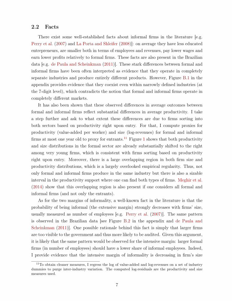
It has also been shown that these observed differences in average outcomes betweenformal and informal firms reflect substantial differences in average productivity. I takea step further and ask to what extent these differences are due to firms sorting intoboth sectors based on productivity right upon entry. For that, I compute proxies forproductivity (value-added per worker) and size (log-revenues) for formal and informalfirms at most one year old to proxy for entrants.11 Figure 1 shows that both productivityand size distributions in the formal sector are already substantially shifted to the rightamong very young firms, which is consistent with firms sorting based on productivityright upon entry. Moreover, there is a large overlapping region in both firm size andproductivity distributions, which is a largely overlooked empirical regularity. Thus, notonly formal and informal firms produce in the same industry but there is also a sizableinterval in the productivity support where one can find both types of firms. Meghir et al.(2014) show that this overlapping region is also present if one considers all formal andinformal firms (and not only the entrants).

As for the two margins of informality, a well-known fact in the literature is that theprobability of being informal (the extensive margin) strongly decreases with firms’ size,usually measured as number of employees [e.g. Perry et al. (2007)]. The same patternis observed in the Brazilian data [see Figure B.2 in the appendix and de Paula andScheinkman (2011)]. One possible rationale behind this fact is simply that larger firmsare too visible to the government and thus more likely to be audited. Given this argument,it is likely that the same pattern would be observed for the intensive margin: larger formalfirms (in number of employees) should have a lower share of informal employees. Indeed,I provide evidence that the intensive margin of informality is decreasing in firm’s size

11To obtain cleaner measures, I regress the log of value-added and log-revenues on a set of industrydummies to purge inter-industry variation. The computed log-residuals are the productivity and sizemeasures used.

7

Figure 1: Productivity and size distributions among entrants

(a) Productivity: Log(VA/Worker)

(b) Size: Log(Revenues)

Notes: Data from ECINF. I regress the log of value-added per worker and log-revenues on a set ofindustry dummies to purge inter-industry variation. The figures show the densities of computedlog-residuals for formal and informal firms.

(Figure B.2 in the appendix).Finally, I assess the empirical relevance of the intensive margin, which can only be done

indirectly with the data available. In Table 2, I use data from the Monthly EmploymentSurvey (PME) to show that 52% of all informal workers are employed in firms with11 employees or more. However, as already discussed, the likelihood of a firm with 11employees or more to be informal is very low. These two pieces of evidence combinedthus suggest that there is a large fraction of informal workers who are employed in formalfirms.

8

Table 2: Formal and informal employment composition by firm size

Informal Workers (in %) Formal workers (in %)

Firm size (# employees)

0–5 35.8 6.6

6–10 11.7 7.2

11 or more 52.5 86.2

Source: Author’s own tabulations from the Monthly Employment Survey (PME) 2003.

3 Theory

Motivated by the facts previously discussed, this section develops an equilibrium entrymodel where firms can exploit both the extensive and intensive margins of informality.Firms are heterogeneous and indexed by their individual productivity, θ. Firms producea homogeneous good using labor as their only input. Product and labor markets are com-petitive, and formal and informal firms face the same prices.12 To simplify the exposition,I assume that workers are homogeneous and formal and informal employees perform theexact same task within the firm.13

3.1 Incumbents

Incumbents in both sectors have access to the same technology. Output of a givenfirm θ is given by y (θ, `) = θq (`), where the function q (·) is a assumed to be increasing,concave, and twice continuously differentiable.

Informal incumbents are able to avoid taxes and labor costs, but face a probability ofdetection by government officials. This expected cost takes the form of a labor distortiondenoted by τi (`), where 1 ≤ τi (·) < ∞, and it is assumed to be increasing and convexin firm’s size (τ ′i , τ ′′i > 0). These assumptions can be rationalized, for instance, by thefact that larger firms have a greater probability of being caught [e.g. Fortin et al. (1997),de Paula and Scheinkman (2011) and Leal Ordonez (2014)].14 Informal firms’ profit

12As argued in Section 2, formal and informal firms coexist even within narrowly defined industries,so the assumption that firms face the same output price seems like a reasonable approximation. Nev-ertheless, the model can be readily modified to a monopolistic competition setting where firms producedifferent varieties.

13Worker homogeneity is a strong assumption, which implies among other things that formal andinformal workers receive the same market wage. Nevertheless, as long as there is positive assortativematching between workers and firms, the results here remain largely unaltered.

14The general cost function τi(·) can be directly obtained from a formulation that explicitly accountsfor a detection probability [see Ulyssea (2014)].

9

function is thus given by:

Πi (θ, w) = max`{θq(`)− wτi (`)} (1)

where the price of the final good is normalized to one.Formal incumbents must comply with taxes and regulations, but they can hire infor-

mal workers to avoid the costs implied by the labor legislation. The hiring costs of formaland informal workers differ due to institutional reasons: formal firms have to pay a con-stant payroll tax on formal workers, while they face an increasing and convex expectedcost to hire informal workers, which is summarized by the function τfi (·), τ ′fi, τ ′′fi > 0 and1 ≤ τfi (·) < ∞. The cost for formal firms of hiring informal workers is thus given byτfi(`)w, while the cost of hiring formally is (1 + τw)w, where τw is the labor tax. Sinceformal and informal workers are perfect substitutes, on the margin firms hire the cheapestone, and hence there is an unique threshold ˜ above which formal firms only hire formalworkers (on the margin).15 Formal firms’ profit function can be written as follows:

Πf (θ, w) = max`{(1− τy) θq(`)− C (`)} (2)

and

C (`) =

τfi (`)w, for ` ≤ ˜

τfi

(˜)w + (1 + τw)w

(`− ˜

), for ` > ˜

(3)

where τy denotes the revenue tax. Incumbents in both sectors must pay a per-period,fixed cost of operation, which is denoted by cs, s = i, f . This a standard formulation inthe literature and can be interpreted as the opportunity cost of operating in sector s. Theprofit function net of this fixed cost of operation is denoted by πs (θ, w) = Πs (θ, w)− cs.

The two margins of informality introduce a size-dependent distortion in the economy,as lower productivity (smaller) firms face de facto lower marginal costs. By the sameargument, more productive, larger firms are more likely to be formal, as the costs ofthe extensive margin of informality are increasing in firm’s size (τ ′i , τ ′′i > 0). Since formalfirms only hire formal workers in excess of ˜, the share of informal workers within a formalfirm is also monotonically decreasing in firm’s size (as observed in the data). Thus, this

15 The marginal cost of hiring informal workers[wτ ′fi(`)

]is strictly increasing, while the marginal

cost of hiring formal workers [(1 + τw)w] is constant. Hence, there is an unique value of ` such thatτ ′fi(˜) = 1 + τw. If the labor quantity that maximizes formal firm’s profit is such that `∗ ≤ ˜, then itwill only hire informal workers. If `∗ > ˜, then the firm will hire ˜ informal workers and `∗ − ˜ formalworkers.

10

highly tractable formulation is able to capture the main facts discussed in the previoussection regarding both margins of informality.16

3.2 Entry

Every period there is a large mass of potential entrants of size M . Potential entrantsonly observe a pre-entry productivity parameter, ν ∼ G, which can be interpreted asa noisy signal of their effective productivity. G is assumed to be absolutely continuouswith support (0,∞), with finite moments, and it is the same for all firms and independentacross periods (i.e. ν is i.i.d.). Hence, the mass of entrants in one period does not affectthe composition of potential entrants in the following period. To enter either sector, firmsmust pay a fixed cost (denominated in units of output) that is assumed to be higher inthe formal sector: Ef > Ei.17 After entry occurs, firms draw their actual productivityfrom the conditional c.d.f. F (θ|ν), which is the same in both sectors and independentacross firms. F (θ|ν) is assumed to be continuous in θ and ν, and strictly decreasing inν. Hence, a higher ν implies a higher probability of a good productivity draw after entryoccurs.

Since firms are ex ante heterogeneous but only realize their actual productivity afterentry occurs, the model allows for the possibility of overlap between formal and informalproductivity distributions. Oppositely, the fully static models without uncertainty implyperfect sorting and no overlap between formal and informal firms’ productivity and sizedistributions,18 which is at odds with the data (as shown in Section 2).

If firms are surprised with a low productivity draw θ < θ, where πs(θ, w

)= 0, they

decide to exit immediately without producing. If firms decide to stay, their productivityremains constant forever and they face an exogenous exit probability denoted by κs,s = i, f . Note that this exit probability could also be interpreted as a sector-specificdiscount rate, which could reflect, for example, differential borrowing rates. Aggregateprices remain constant in steady state equilibria and since firms’ productivity also remains

16However, this formulation also implies that all formal firms hire some informal workers (up to ˜),which for very large firms might be unrealistic (even though their share of informal workers is going tozero). Nevertheless, given that the model captures well the behavior of the share of informal workerswithin formal firms, the gains in tractability justify this modeling option.

17The difference between these entry costs is interpreted here as a consequence of the regulation ofentry into the formal sector (e.g. red tape bureaucracy). Under this interpretation, the entry cost intothe informal sector can be seen as the initial investment or minimum scale required to operate in thegiven industry.

18See, for example, Rauch (1991), Fortin et al. (1997), de Paula and Scheinkman (2011), Prado (2011),and Galiani and Weinschelbaum (2012).

11

constant, firm’s value function assumes a very simple form:

Vs (θ, w) = max

{0,πs (θ, w)

κs

}where for notational simplicity I assume that the discount rate is normalized to one. Theexpected value of entry for a firm with pre-entry signal ν is thus given by

V es (ν, w) =

∫Vs (θ, w) dF (θ|ν) , s = i, f (4)

Entry into the formal sector occurs if V ef (ν, w)−Ef ≥ max {V e

i (ν, w)− Ei, 0}, whileentry into the informal sector occurs if V e

i (ν, w)−Ei > max{V ef (ν, w)− Ef , 0

}. If entry

in both sectors is positive the following entry-conditions hold:

V ei (νi, w) = Ei

V ef (νf , w) = V e

i (νf , w) + (Ef − Ei)

where νs is the pre-entry productivity of the last firm to enter sector s = i, f . The ap-pendix D.1 shows that the effective, post-entry productivity distributions in both sectorscan be derived as functions of these thresholds.

3.3 Equilibrium

To close the model, it is necessary to specify the demand side of the model. I assumethat there is a representative household that inelastically supplies L units of labor andthat derives utility solely from consuming the final good, x:

U =∞∑t=0

βtu (xt)

The focus lies on stationary equilibria, where all aggregate variables remain constant.In a stationary equilibrium with constant prices the household problem simplifies to astatic optimization problem:

maxx

u (x) s.t. x ≤ wL+ Π + T (5)

The Π denotes total profits in the economy net of total entry costs, MfEf + MiEi,where Mi = [G (νf )−G (νi)]M and Mf = [1−G (νf )]M denote the measures of en-trants into the informal and formal sectors, respectively. The T denotes tax revenues,which are directly transferred to households. Consumers do not derive any disutility from

12

work and cannot save, so they simply consume all their income. Total consumption thusconstitutes the natural welfare measure in this context, which in equilibrium is given byW = wL+ Π + T .

In a stationary equilibrium, the size of the formal and informal sectors must remainconstant over time, which implies the following condition:

µs =1− Fθs

(θs)

κsMs (6)

where µs denotes the mass of active firms in sector s. In words, condition (6) simplystates that the mass of successful entrants in both sectors must be equal to the mass ofincumbents that exit.

In sum, the equilibrium conditions are given by the following: (i) markets clear,Li + Lf = L; (ii) The zero profit cutoff (ZPC) condition holds in both sectors, θ ≥ θs

where πs(θs, w

)= 0; (iii) the free entry condition holds in both sectors, with equality if

Ms > 0; and (iv) both sectors’ size remains constant (expression 6). Appendix D.2 showsthat the equilibrium exists and it is unique.

4 A Taxonomy of Informal Firms

In this section I propose a simple taxonomy of informal firms based on the three maincompeting views that exist in the literature [see La Porta and Shleifer (2008, 2014) for adiscussion]. The starting point of the analysis is to establish a precise definition of eachtype, which comes directly from these views:

• Survival view (type 1): Informal firms that are too unproductive to ever becomeformal, even if entry costs were removed. These are entrepreneurs with low humancapital, who are only able to survive in the informal sector because they avoid taxesand regulations.

• Parasite view (type 2): Informal firms that are productive enough to survive asformal firms once entry barriers are removed, but choose not to do so because it ismore profitable for them to remain informal.

• De Soto’s view (type 3): Higher productivity informal firms that are kept out offormality by high entry costs. If these were removed, they would become formaland improve their performance, as they would no longer have the size constraintsimposed by informality.

13

The crucial difference between these types is how they would respond to a policythat eliminates entry costs into the formal sector. Type 3 firms would formalize theirbusiness and would be better off in this counter-factual scenario, as they are no longerconstrained by the growth limitations imposed by informality. Hence, any model thatdoes not account for entry costs into the formal sector cannot account for this view, asthere would be no bunching of informal firms near the transition threshold. However, theother two types are not so easily distinguishable, as both are predicted to remain informalin the absence of entry costs. Any model that has firms sorting between sectors, evenwithout entry costs and productivity uncertainty, would be able to account for these twotypes. The crucial differentiation between Types 1 and 2 is the reason why they remaininformal. Type 2 firms are productive enough to survive in the formal sector (once entrybarriers are removed), but choose to remain informal to receive higher profits. Type 1firms are simply not productive enough to be formal, and are only able to survive due tothe cost advantages of non-compliance.

Given this reasoning, it is possible to represent the different types using the modeljust discussed. The thought experiment is to ask how informal firms would respond toan intervention that equalizes entry costs in the formal and informal sectors (Ef = Ei).To disentangle types 1 and 2 it is necessary to ask a somewhat harder question: Whichfirms could actually become formal in the counter-factual scenario but choose not todo it? Figure 2 summarizes this thought experiment. For each post-entry productivitylevel (θ),19 it plots firm’s post-entry value function net of entry costs in both sectors atbaseline, Vs(θ) − Es, and the value of being formal under the counter-factual scenariowhere formal and informal sectors’ entry costs are equalized, V c

f (θ) − Ei, where thesuperscript c indicates the counter-factual scenario.20

The baseline curves for the formal and informal sectors intersect each other at θ = θ3,and all firms with θ ≥ θ3 will always choose to be formal, as their value is higher thanbeing informal. Firms with productivity θ ∈ [θ2, θ3) are the De Soto’s (type 3) firms:once entry barriers into the formal sector are removed, they migrate to the formal sector,improve their performance and achieve higher profits. Firms with productivity θ ∈ [θ1, θ2)

correspond to Parasite (type 2) firms: They are productive enough to produce in theformal sector – their value in the formal sector is everywhere above zero – but choose notto do it to obtain higher returns in the informal sector. Finally, firms with θ < θ1 are theSurvival (type 1) firms, which are not productive enough to go to the formal sector even

19Firms make entry decisions and sort between sectors based on their pre-entry signal, ν, and afterentry occurs they realize their actual productivity, θ, which is drawn from F (θ|ν).

20To obtain these curves it is necessary to specialize the model to specific functional forms andparameter values. I postpone this discussion to the following section, where I present the estimationprocedure.

14

Figure 2: Graphic taxonomy of informal firms types

Firm's  Va

lue  F

unc/on

 Net  of  E

ntry  Costs  

Firm's  produc/vity  

Baseline  Net  Value  Func/on:  Informal  Sector  [  Vi(θ)  -­‐  Ei]  

Baseline  Net  Value  Func/on:  Formal  Sector  [  Vf(θ)  -­‐  Ef]  

Counterfactual  Net  Value  Func/on:  Formal  Sector    [  Vf(θ)  -­‐  Ei]  

θ1   θ2   θ3  

0  

De  Soto's  View  

Parasite  View  

Survival  View  

Always  Formal  

Note: The figure shows, for each productivity level, firms’ post-entry baseline value function net of entry costs in theformal and informal sectors, Vf (θ)− Ef and (Vi(θ)− Ei), respectively. The third curve displays the post-entry, net valueof being formal in the counter-factual scenario where formal sector’s entry costs are equated to informal sector’s(Ef = Ei): V cf (θ)− Ei, where the superscript c indicates the counter-factual scenario.

without entry costs, and use informality as a survival strategy.Contrary to what is often argued in the literature,21 Figure 2 shows that these views

are not fundamentally different, they simply reflect firm heterogeneity. Thus, they arecomplementary and not competing frameworks for understanding informality. The crucialquestion is therefore to infer the relative importance of each view in the data. For that,it is necessary to estimate the model and use it to back out the mass of firms in each ofthe θ intervals just described. The following section describes the estimation procedure,while Section 6 describes the quantitative results.

5 Estimation

The model presented in Section 3 describes firms’ decisions regarding entry, productionand compliance with regulations in an equilibrium setting. To perform counter-factualanalysis and make quantitative statements about firms types and how they would respond

21See La Porta and Shleifer (2008, 2014) for a systematic overview of the existing literature regardingthese views.

15

to policy changes, it is necessary to estimate all objects in the model’s structure. I esti-mate the model using a two-stage simulated method of moments (SMM). This approachcombines direct estimation and calibration from micro and macro data in the first stage,with the SMM estimator itself in the second stage [e.g. Gourinchas and Parker (2002)].

To proceed with the estimation, it is first necessary to complete the model’s parame-terization and assume functional forms for the different objects in the model,22 which nat-urally raises identification concerns. However, non-parametric estimation in the presentcontext is either not feasible (given the goals of this paper and the data available), orthe assumptions needed are not attainable.23 The fully parametric approach adoptedhere is thus crucial in order to overcome some data limitations and to provide a richcounter-factual analysis.

5.1 Parameterization

Up to this point, the initial productivity distribution, Gν , the productivity process,F (θ|ν), the production function, q(·), and the cost functions, τs(·), were left unspeci-fied. This section completes the model’s parameterization by assuming specific func-tional forms for these objects. Starting with the pre-entry productivity distribution, it isassumed that it has a Pareto distribution:24

Fν (ν ≥ x) =

(ν0x

)ξ for x ≥ ν0

1 for x < ν0

(7)

Firms’ actual productivity is only determined after entry occurs. I assume a verysimple log-additive form for the post-entry productivity process, which is determined asfollows: θ = εν, where the unexpected shock ε is i.i.d. and has a log-normal distributionwith mean zero and variance σ2. As for production, I assume that firms use a Cobb-Douglas technology: y (θ, l) = θlα, α < 1.

The cost functions of both margins take a very simple functional form: τs(`) =(1 + `

bs

)`, where bs > 0 and s = i, f . Finally, I assume that the per-period, fixed

costs of operation are a function of the equilibrium wage, which makes the exit mar-gin more meaningful since it now responds to market conditions. The fixed costs are

22It is not always the case that one needs to identify all the objects in the model’s structure in orderto answer specific policy questions [see, for example, Heckman (2001) and Ichimura and Taber (2002)].However, ex ante policy evaluations typically require the full specification of a behavioral model in orderto perform the counter-factual analysis [e.g. Keane et al. (2011)].

23See the Web Appendix for a detailed discussion.24A well documented fact in the literature is that the Pareto distribution fits firms’ size distribution

remarkably well, see more recently Luttmer (2007), among others.

16

determined as follows: cs = γsw, 0 < γs ≤ 1.The parameter vector to be estimated is thus given by

Γ = {τw, τy, κf , κi, α, σ, γf , γi, bi, bf , ξ, ν0, Ef , Ei}

which is partitioned into two sub-vectors, Γ = {ψ, ϕ}, the first and second stage param-eters, respectively. The SMM estimator used in the second stage takes the parameters inψ as given in order estimate the vector ϕ. The next subsection describes the estimationsteps.

5.2 Fitting the model to the data

The vector of parameters determined in the first stage is given by

ψ = {τw, τy, κf , ν0, γf}

The tax rates are set to their statutory values: τw = 0.375 and τy = 0.293.25 The exitprobability in the formal sector is κf = 0.129, which is estimated using the panel structurein the RAIS data set. This estimate is obtained using the predicted exit probability forthe average firm in the sample. The Pareto distribution scale parameter (ν0) is set sothat the firms’ minimum size is one employee, while formal sector’s fixed cost of operation(γf = 0.5) is set to be half of the monthly wage.

5.2.1 Second stage: SMM estimation

For a given parameter vector (Γ), wage (w) and individual productivity shocks (νjand εj), one can use the model to completely characterize firms’ behavior. The SMMestimator proceeds by using the model to generate simulated data sets of formal andinformal firms and computing a set of moments that are also computed from real data.The estimate is obtained as the parameter vector that best approximates the momentscomputed from the simulated data to the ones computed from real data.26

Let m denote the vector of moments computed from data, and let ms(ϕ;ψ) denotethe vector of the same moments computed from the simulated data. Define g (ϕ;ψ) =

m−ms(ϕ;ψ); the SMM estimation is based on the moment condition E [g (ϕ0;ψ0)] = 0,

25The value of τw corresponds to the main payroll taxes, namely, employer’s social security contribu-tion (20%), direct payroll tax (9%), and severance contributions (FGTS), 8.5%. The value of τy includestwo VAT-like taxes: the IPI (20%) and PIS/COFINS (9.25%). These values can be easily obtained inthe compilation by the World Bank’s Doing Business initiative.

26The technical details are discussed in the Appendix E.1. The interested reader can find an in-depthand systematized discussion in Gourieroux and Monfort (1996) and Adda and Cooper (2003).

17

where ϕ0 and ψ0 denote the true values of ϕ and ψ, respectively. The second-stage, SMMestimator is then given by

ϕ = arg minϕQ (ϕ;ψ) =

{g (ϕ;ψ)′ Wg (ϕ;ψ)

}(8)

where Wp−→W, and W is a positive semi-definite weighting matrix. Under the suitable

regularity conditions (which are discussed in the web appendix), the SMM estimator isconsistent and asymptotically normal. The Appendix E.1 describes the derivation of theasymptotic variance-covariance matrix and the computation of the optimal W, while theappendix E.2 describes the optimization algorithm.

5.2.2 Moments and identification

There are 9 (nine) parameters to be estimated in the second stage:

ϕ = {κi, γi, bi, bf , ξ, α, Ef , Ei, σ}

I use 18 moments from the data to form the vector m,27 which are the following: (i)share of informal employees (data source: PNAD); (ii) overall share of informal firmsand by firm size for n = 1, ..., 5, where n is the number of employees (data sources:ECINF and RAIS); (iii) average share of informal workers within formal firms with sizen = 2, ..., 5 (data source: ECINF); (iv) the 75th, 95th and 99th percentiles of informalfirms’ size distribution (for firms with up to 5 employees – data from ECINF); and (v)the 25th, 50th, 75th and 95th percentiles of formal firms’ size distribution (data source:RAIS).

Even though simulation-based methods typically do not allow for formal identificationarguments, it is possible to discuss the role that some moments play in the identificationof different parameters [e.g. Dix-Carneiro (2014)]. The shape parameter of the Paretodistribution, ξ, is completely determined by the moments of firm size distribution. Infact, given the one-to-one relationship between productivity and firms’ size in the model,estimation of the productivity distribution crucially relies on observed moments of firmsize distribution (measured by number of employees).

As for the parameters that govern the cost functions of both margins of informality,

27As discussed in Section 2, the data sets used are the following: ECINF (Pesquisa de EconomiaInformal Urbana), a repeated cross-section of small firms (up to five employees), collected by the BrazilianBureau of Statistics (IBGE); RAIS (Relação Anual de Informações Sociais), an administrative data setfrom the Ministry of Labor, which provides an annual panel with the universe of formal firms andworkers; and PNAD, the National Household Survey, a repeated cross section that is representative atthe national level.

18

the share of informal firms by firm size plays a crucial role in identifying bi, while the shareof informal workers in formal firms by firm size identifies bf . As for informal sector’s exit(or discount) rate κi, it determines the overall disadvantage of being informal relatively tobeing formal, because a higher κi represents an overall downward shift in informal firms’value function. Thus, given formal sector’s entry cost, κi is disciplined by the overallshare of informal firms. Given γf (determined in the first stage), γi and the post-entryshock (σ) are largely determined by the degree of overlap between formal and informalfirm size distributions, and the minimum size of entrants in the informal sector. Formalsector’s entry cost (Ef ) is disciplined by the minimum entry size among formal firms andhow shifted to the right firm size distribution is relatively to informal sector’s. Similarly,informal sector’s entry cost is likely to be determined by entrants’ minimum scale, whichcomes from the lower percentiles of firm size distribution in the informal sector.

5.2.3 Estimates and Model Fit

Table 3 shows the values of both first and second stage parameters, ψ and ϕ respec-tively. The estimates show that formal sector’s entry cost is more than twice informalsector’s. Exit (discount) rate in the informal sector is also more than twice as high asformal sector’s, which confirms the anecdotal evidence that informal firms have higherturnover rates than their formal counterparts. Pareto’s shape parameter, ξ, indicatesthat the productivity distribution is skewed to the left, as observed in the data for firmsize.

As for the fit of the model, Table 4 shows how the model performs compared to theobserved moments in the data. The model matches the share of informal firms and theshare of informal workers well. However, it understates the share of informal firms withonly one employee (the 75% percentile of the actual size distribution in the informalsector). The same does not happen with the size distribution in the formal sector, whichthe model is able to replicate well. The main reason for this greater accuracy in estimatingformal sector’s firm size distribution is that the corresponding empirical moments aremore precisely estimated using RAIS, and therefore they receive larger weights in theoptimal weighting matrix W (see the discussion in Appendix E.1).

19

Table 3: Parameter Values

Parameter Description Source Value SE

First Stage

τw Payroll Tax Statutory values 0.375 –

τy Revenue Tax Statutory values 0.293 –

κf Formal Sector’s Exit Probability Panel Estimation 0.129 –

ν0 Pareto’s Location Parameter Calibrated 7.7 –

γf Per-period fixed cost of operation (Formal) Calibrated 0.5 –

Second Stage

α Cobb-Douglas Coefficient Estimated (SMM) 0.649 0.003

bf Intensive Mg. Cost: τfi(`) =(

1 + `bf

)` Estimated (SMM) 4.592 0.127

bi Extensive Mg Cost: τi(`) =(

1 + `bi

)` Estimated (SMM) 4.522 0.038

κi Informal Sector’s Exit Probability Estimated (SMM) 0.349 0.017

γi Per-period fixed cost of operation (Informal) Estimated (SMM) 0.246 0.035

ξ Pareto’s Shape Parameter Estimated (SMM) 3.9 0.064

σ Post-Entry Shock Variance Estimated (SMM) 0.141 0.005

Ef† Formal Sector’s Entry Cost Estimated (SMM) 6,077 372

Ei† Informal Sector’s Entry Cost Estimated (SMM) 2,550 177.2

† Estimates and SD expressed in R$ of 2003.

20

Table 4: Model fit

Moments Source Data Model

Share inf. workers PNAD 0.354 0.352

Share inf. Firms ECINF & RAIS 0.686 0.695

Size Distribution: Informal Firms

≤ 1 employee ECINF 0.849 0.481

≤ 2 employees ECINF 0.958 0.946

≤ 4 employees ECINF 0.993 0.995

Size Distribution: Formal Firms

≤ 1 employee RAIS 0.295 0.299

≤ 3 employees RAIS 0.563 0.545

≤ 7 employees RAIS 0.774 0.784

≤ 31 employees RAIS 0.953 0.959

Notes: PNAD is the National Household Survey, a repeated cross-section available an-nually; ECINF (Pesquisa de Economia Informal Urbana) is a repeated cross-section ofsmall firms (up to five employees), available only for 1997 and 2003; both data sets arecollected by the Brazilian Bureau of Statistics (IBGE). RAIS (Relacao Anual de Infor-macoes Sociais) is an administrative data set collected by the Ministry of Labor, whichprovides an annual panel with the universe of formal firms and workers. All momentsare computed using data from 2003, which is the last year ECINF is available.

21

6 Quantitative results

6.1 The distribution of informal firms’ types in the data

In this section I use the estimation results and the taxonomy discussed in Section4 to back out from the data the distribution of informal firms’ types. For that, I usethe estimated model to obtain, for each firm θ, the baseline net value function of beingformal and informal: Vf (θ)−Ef and Vi(θ)−Ei, respectively. I then simulate the counter-factual scenario where entry costs into the formal sector are equalized to informal sector’s(Ef = Ei), and compute for all firms the counter-factual value of being formal once entrycosts are removed, which is given by V c

f (θ) − Ei, where again the superscript c denotesthe counter-factual scenario. Figure 3 revisits Figure 2 by displaying the correspondingempirical curves.

Figure 3: The distribution of informal firms types in the data

Firm's  Va

lue  F

unc/on

 Net  of  E

ntry  Costs  

Firm's  produc/vity  

Baseline  Net  Value  Func/on:  Informal  Sector  [  Vi(θ)  -­‐  Ei]  

Baseline  Net  Value  Func/on:  Formal  Sector  [  Vf(θ)  -­‐  Ef]  

Counterfactual  Net  Value  Func/on:  Formal  Sector    [  Vf(θ)  -­‐  Ei]  

θ1   θ2   θ3  

0  

De  Soto's  View  

=  16.8%  

Parasite  View  

=  38.7%  

Survival  View  

=  44.5%  

Note: The figure shows, for each productivity level, firms’ value function net of entry costs in the formal and informalsectors, Vf (θ)− Ef and Vi(θ)− Ei, respectively. The third curve displays the net value of being formal in a scenariowhere entry costs into the formal sector are equalized to informal sector’s (Ef = Ei): V cf (θ)− Ei, where the primeindicates the counterfactual scenario.

The relative sizes of each view are obtained by computing the mass of firms withineach of the three intervals. Hence, they crucially depend on the effective productivitydistribution in the informal sector, which is determined by three main elements: (i) theunderlying pre-entry productivity distribution Fν ; (ii) the determinants of firms’ sorting

22

between sectors; and (iii) the selection mechanism after entry occurs, which selects outthe least productive firms.28 As discussed in the previous section, the parameters thatgovern (i) and (iii) are identified by firm size distributions in both sectors and the degreeof overlap between them. Element (ii) is determined by the interplay between the pre-entry productivity distribution, entry costs, and the institutional factors that determineexpected profitability in both sectors, such as taxes and the costs of both margins ofinformality.

The data indicates that the potentially productive informal firms that are kept out offormality by high entry costs (De Soto’s view) are the minority, corresponding to 16.8%of all informal firms. Parasite (type 2) firms, those that could survive as formal firmsonce entry costs are removed but choose to remain informal to enjoy the cost advantagesof non-compliance correspond to 38.7% of all informal firms. The remaining firms, 44.5%,correspond to the survival view (type 1) firms, which are too unproductive to ever becomeformal and are only able to survive in the informal sector. These results thus suggestthat eradicating informal firms through higher enforcement would be a more effectivepolicy to reduce informality and improve economic performance than simply reducingentry costs. In the following section I examine the firm-level and aggregate impacts ofdifferent policies towards informality.

6.2 Firm-level and aggregate impacts of formalization policies

In this section I analyze the impacts of formalization policies at the firm level andhow they aggregate up to different economy-wide effects. I consider four experiments:(i) equalizing formal and informal sectors’ entry costs; (ii) a 20 p.p. cut in the payrolltax (which corresponds to eliminating social security contribution); (iii) increasing thecost of being an informal firm (the extensive margin); and (iv) increasing formal firms’costs of hiring informal workers (the intensive margin). The latter two could be achievedthrough greater monitoring efforts by the government, which in the model translates intolower values of the parameter bs, s = i, f . In what follows I analyze the effects at thefirm and aggregate levels separately.

6.2.1 The impacts on firms

To analyze the effects on firms, I follow the policy evaluation literature and use themarginal treatment effect (MTE) as impact measure [e.g. Heckman and Vytlacil (2005)].The outcome considered here is firm’s post-entry value function, V (θ), net of entry costs.

28The Appendix D.1 contains the derivation of post-entry productivity distributions.

23

For firms that remain in the same sector both in the baseline and counter-factual scenar-ios, the MTE is simply given by

∆(θ;Stayers) = log (V cs (θ))− log (Vs(θ)) (9)

where again θ denotes firm’s productivity, the superscript c denotes the counter-factualscenario, and s = i, f indexes firm’s sector (formal and informal).

Firms that are informal in the baseline and decide to switch to the formal sectorin the counter-factual scenario must pay the difference in entry costs between sectors,E = Ef − Ei. Their net, counter-factual payoff in the formal sector will be V c

f (θ) − E,and the MTE for switchers can thus be written as:

∆(θ;Switchers) = log(V cf (θ)− E

)− log (Vi(θ)) (10)

Therefore, firms can be divided into three basic groups: (i) formal stayers, which arethose that are formal in the baseline and choose to remain formal in the counter-factualscenario; (ii) informal stayers, which are informal in both the baseline and counter-factualscenarios; and (iii) movers, which are the informal firms that choose to formalize after thepolicy is implemented. I start by analyzing the MTE-productivity profiles within eachof these groups of firms and for all four policy interventions considered. For each policyand group, I compute the average MTE at the points in firms’ productivity grid. Figure4 shows the profiles for the policies that seek to reduce regulatory costs – entry costs andpayroll tax – which correspond to policies (i) and (ii) above. Figure 5 shows the profilesfor policies (iii) and (iv), which increase the costs of the extensive and intensive marginsof informality, respectively.

Figure 4 [panel (a)] shows that all formal incumbents are hurt when formal sector’sentry costs are reduced, but specially the less productive ones. This is due to the factthat reducing entry costs induces greater entry into the formal sector, which increasescompetition and therefore the equilibrium wage (Table 6). Because of these generalequilibrium effects on wages, informal incumbents are also negatively affected by thispolicy [panel (c)], with a larger negative effect on average (Table 5). Turning to thepayroll tax reduction, it substantially hurts low productivity formal incumbents but ithas positive impacts on high productivity ones, with the MTE increasing monotonicallyfrom the lowest to the highest productivity firm [panel (b)]. This negative effect on lowproductivity formal firms and on all informal incumbents [panel (d)] once again comesfrom the general equilibrium effects on wages: as the payroll tax decreases the demand forlabor increases, leading to a strong positive effect on the equilibrium wage. Due to this

24

Figure 4: Profiles of Marginal Treatment Effects: Reducing regulatory costs

(a) Equalizing entry costs: Formal stayers (b) Reducing Payroll Tax: Formal Stayers

(c) Equalizing entry costs: Informal stayers (d) Reducing Payroll Tax: Informal Stayers

(e) Equalizing entry costs: Movers (f) Reducing Payroll Tax: Movers

25

Figure 5: Profiles of Marginal Treatment Effects: Increasing the costs of informality

(a) Extensive Margin: Formal stayers (b) Intensive Margin: Formal Stayers

(c) Extensive Margin: Informal stayers (d) Intensive Margin: Informal Stayers

(e) Extensive Margin: Movers

26

wage increase, low productivity firms reduce their scale and resources are shifted awayfrom these firms to more productive ones, which explains the increasing MTE profileobserved in panel (b). Finally, informal firms that formalize due to either policy – panels(e) and (f) – greatly benefit from it, with an average increase in firms’ value function ofnearly 24% in the entry cost experiment and 13.2% in the payroll tax experiment (Table5). As Table 5 shows, there is a large degree of heterogeneity in the MTEs for movers,specially in the payroll tax experiment, where the effects range from a 0.7% gain in firms’value function (the 25th and 50th percentiles) to a 54.9% gain in the 95th percentile of theMTE distribution.

Turning to the experiments that increase the costs of informality, Figure 5 [panel (a)]shows that formal incumbents benefit from higher enforcement on the extensive marginof informality, with an average increase of 4.9% in their value functions (Table 5). In-terestingly, low-productivity formal firms benefit the most, which indicates that they arethe ones most directly affected by the competition from informal firms. Increasing en-forcement on the extensive margin induces some informal firms to formalize and displacesa large share of informal firms. Those that survive have to greatly reduce their scale inorder to stay invisible to the government, which causes them to experience a very largenegative impact, with an average reduction of 66.4% in their value functions (Table 5).

Increasing the costs of the intensive margin of informality is most harmful to lowproductivity formal firms, as these firms hire a large fraction of their labor force without aformal contract. Thus, increasing enforcement on this margin of informality substantiallyincreases effective labor costs for these firms. On the contrary, this policy has verylimited impacts on informal firms albeit slightly positive. This result comes from generalequilibrium effects, which lead to a small reduction in the equilibrium wage due to a lowerdemand for labor from low productivity formal firms.

6.2.2 Economy-wide effects

Reducing formal sector’s entry cost leads to a substantial reduction in the share ofinformal firms, of nearly 22 p.p. (Table 6). The effect on the share of informal workersis however nearly null, which highlights the importance of accounting for the intensivemargin of informality: the share of formal firms grows due to the formalization of low-productivity firms, which hire a large share of their labor force without a formal contract,and therefore the net effect on labor informality is near zero.

The opposite is true when the payroll tax is reduced: informal employment is sub-stantially reduced but the share of informal firms does not fall as much. This is observedbecause the labor tax directly affects formal firms’ decision to hire informal or formal la-

27

Table 5: The Distribution of Marginal Treatment Effects

All Firms Formal Stayers Informal Stayers Movers

Reducing Entry Costs

Mean -0.088 -0.071 -0.105 0.215Pctile 25 -0.054 -0.076 -0.045 0.120Pctile 50 -0.043 -0.064 -0.043 0.192Pctile 75 -0.038 -0.058 -0.038 0.324Pctile 95 -0.033 -0.054 -0.035 0.448

Reducing Payroll Tax

Mean -0.173 -0.045 -0.197 0.124Pctile 25 -0.212 -0.095 -0.212 0.007Pctile 50 -0.191 -0.023 -0.200 0.007Pctile 75 -0.167 0.015 -0.174 0.246Pctile 95 0.007 0.038 -0.155 0.438

Higher Enforcement - Extensive Mg.

Mean -0.793 0.048 -1.091 -0.165Pctile 25 -1.092 0.040 -1.105 -0.510Pctile 50 -1.074 0.044 -1.092 -0.143Pctile 75 -0.306 0.051 -1.074 0.112Pctile 95 0.068 0.076 -1.066 0.399

Higher Enforcement - Intensive Mg.

Mean -0.009 -0.072 0.001 –Pctile 25 0.001 -0.100 0.001 –Pctile 50 0.001 -0.059 0.001 –Pctile 75 0.001 -0.026 0.001 –Pctile 95 0.001 -0.006 0.001 –

Note: The MTEs are computed used the expressions (9) and (10), defined in thetext.

bor; however, firms’ formalization is also heavily influenced by formal sector’s entry cost,which remains unaltered. Increasing enforcement on the intensive margin is the leasteffective policy to reduce informality, as it only generates a small reduction in the shareof informal workers and leads to greater informality among firms. The latter effect isobserved because the effective cost of being formal increases for less productive firms, asit is now harder for formal firms to hire informal workers, which increases their incentivesto become informal.

These subtler policy impacts can only be unveiled if one explicitly considers the in-tensive margin. The existing literature has focused on the extensive margin alone, andtherefore reducing firm informality necessarily leads to lower labor informality. As theabove results show, this is no longer the case if one accounts for the intensive margin, and

28

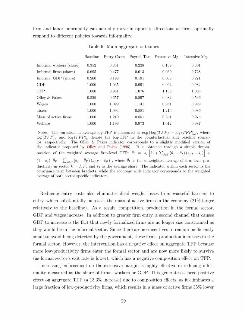
firm and labor informality can actually move in opposite directions as firms optimallyrespond to different policies towards informality.

Table 6: Main aggregate outcomes

Baseline Entry Costs Payroll Tax Extensive Mg. Intensive Mg.

Informal workers (share) 0.352 0.351 0.228 0.138 0.301

Informal firms (share) 0.695 0.477 0.613 0.039 0.728

Informal GDP (share) 0.260 0.198 0.191 0.005 0.271

GDP 1.000 1.035 0.991 0.994 0.984

TFP 1.000 0.951 1.076 1.133 1.005

Olley & Pakes 0.559 0.657 0.597 0.684 0.536

Wages 1.000 1.029 1.141 0.981 0.999

Taxes 1.000 1.094 0.881 1.216 0.986

Mass of active firms 1.000 1.210 0.851 0.651 0.975

Welfare 1.000 1.199 0.973 1.012 0.987

Notes: The variation in average log-TFP is measured as exp {log (TFP )c − log (TFP )b}, wherelog (TFP )c and log (TFP )b denote the log-TFP in the counterfactual and baseline scenar-ios, respectively. The Olley & Pakes indicator corresponds to a slightly modified version ofthe indicator proposed by Olley and Pakes (1996). It is obtained through a simple decom-position of the weighted average firm-level TFP: Θ = sI

[θI +

∑j∈I

(θj − θI

)(sj,I − sI)

]+

(1− sI)[θF +

∑j∈F

(θj − θF

)(sj,F − sF )

], where θk is the unweighted average of firm-level pro-

ductivity in sector k = I, F , and sk is the average share. The indicator within each sector is thecovariance term between brackets, while the economy wide indicator corresponds to the weightedaverage of both sector specific indicators.

Reducing entry costs also eliminates dead weight losses from wasteful barriers toentry, which substantially increases the mass of active firms in the economy (21% largerrelatively to the baseline). As a result, competition, production in the formal sector,GDP and wages increase. In addition to greater firm entry, a second channel that causesGDP to increase is the fact that newly formalized firms are no longer size constrained asthey would be in the informal sector. Since there are no incentives to remain inefficientlysmall to avoid being detected by the government, these firms’ production increases in theformal sector. However, the intervention has a negative effect on aggregate TFP becausemore low-productivity firms enter the formal sector and are now more likely to survive(as formal sector’s exit rate is lower), which has a negative composition effect on TFP.

Increasing enforcement on the extensive margin is highly effective in reducing infor-mality measured as the share of firms, workers or GDP. This generates a large positiveeffect on aggregate TFP (a 13.3% increase) due to composition effects, as it eliminates alarge fraction of low-productivity firms, which results in a mass of active firms 35% lower

29

than in the baseline. The GDP remains roughly unchanged, which is a consequence ofthese two opposing effects: higher TFP going in the direction of increasing productionand lower mass of firms in the opposite direction.

The welfare analysis shows that reducing entry costs leads to a substantial welfaregain of nearly 20%. This result is a consequence of the substantial increase in the mass ofactive firms, higher GDP, wages and tax revenues; additionally, this policy mechanicallyincreases aggregate net profits (which enters directly the welfare measure), as formalsector’s entry costs are substantially reduced. Higher enforcement on the extensive marginalso has a positive but smaller effect on welfare (a 1.2% increase), which is a result of twocounteracting forces. On the one hand, it leads to a substantial increase in tax revenues(21.6%), which is rebated directly to the households.29 On the other hand, this policyeradicates almost all informal firms, substantially reducing the mass of active firms, andreduces the equilibrium wage. It is worth highlighting that this should be seen as anupper bound for the impacts of greater enforcement on welfare, as the experiment makestwo strong assumptions: (i) all tax revenues are directly rebated to households, with noresources lost; and (ii) there is no cost of implementing greater enforcement. The latteris likely to be substantial, since monitoring a large number of small firms is likely to becostly.

Finally, even though the different interventions always manage to reduce at least onemeasure of informality, they do not always lead to welfare improvements. This is the caseof higher enforcement on the intensive margin and lower payroll tax. In the first case, thepolicy reduces the share of informal workers but negatively affects small formal firms andactually leads to an increase in the share of informal firms. These effects, combined witha slight decline in tax revenues, cause welfare to decrease. As for the lower payroll taxintervention, its general equilibrium effects (i.e. wage increases) undo some its firm-levelbenefits. More importantly, there is a substantial reduction in tax revenues, which hasdirect negative impacts on welfare.

7 Final remarks

This paper investigates the role of informal firms in economic development, how theyrespond to different formalization policies and their effects on overall economic perfor-mance. I develop a framework that distinguishes between two margins of informality: (i)when firms do not register and pay entry fees (extensive margin); and (ii) when firmspay workers "off the books" (intensive margin). The latter is a central innovation, as it

29This positive effect can be interpreted as a stylized version of the mechanisms highlighted by theliterature on fiscal capacity [e.g. Besley and Persson (2013)].

30

is empirically important and allows to unveil new and non-obvious firm-level responsesto policy changes regarding informality decisions. Accounting for the intensive marginalso has direct implications to our understanding of informality, as it breaks the directassociation between worker and firm informality. In particular, formal and informal areno longer disjoint states for firms, as formal firms may hire part or all of their labor forceinformally.

The framework developed here integrates the leading views of informality in an unifiedsetting, and provides a natural taxonomy of informal firms based on these views. I takethe model to data on formal and informal firms in Brazil to back out the empiricalrelevance of these competing views. The results show that firms that are potentiallyproductive and which formalize and succeed when formal sector’s entry costs are removedconstitute a small fraction of all informal firms (16.8%). The view that argues thatinformal firms choose informality to exploit the cost advantages of non-compliance eventhough they are productive enough to survive in the formal sector corresponds to alarge fraction of all informal firms, 38.7%. The remaining firms correspond to those toounproductive to ever become formal.

Counterfactual analysis of policy effects shows that no single policy generates positiveeffects for all firms and that there is substantial heterogeneity in policy effects betweengroups (i.e. informal to formal switchers, formal stayers and informal stayers) and withingroups. At the aggregate level, I find that increasing enforcement is highly effectivein reducing informality but it does not increase GDP and barely increases welfare (anupper bound effect of 1.2%). Reducing formal sector’s entry costs is not as effective inreducing informality but generates substantial welfare gains and leads to greater GDPand wages. Overall, the results show that informality reductions can be but are notnecessarily associated to higher GDP, TFP or welfare.

References

Abbring, J. H. (2010). Identification of dynamic discrete choice models. Annual Reviewof Economics 2 (1), 367–394.

Ackerberg, D., C. L. Benkard, S. Berry, and A. Pakes (2007). Econometric tools foranalyzing market outcomes. Handbook of econometrics 6, 4171–4276.

Adamopoulos, T. and D. Restuccia (2013). The size distribution of farms and interna-tional productivity differences. American Economic Review . Forthcoming.

31

Adda, J. and R. Cooper (2003). Dynamic Economics: Quantitative methods and appli-cations. The MIT Press.

Aguirregabiria, V. and P. Mira (2010). Dynamic discrete choice structural models: Asurvey. Journal of Econometrics 156 (1), 38–67.

Almeida, R. and P. Carneiro (2009). Enforcement of labor regulation and firm size.Journal of Comparative Economics 37 (1), 28 – 46.

Almeida, R. and P. Carneiro (2012). Enforcement of labor regulation and informality.American Economic Journal: Applied Economics 4 (3), 64–89.

Amaral, P. S. and E. Quintin (2006). A competitive model of the informal sector. Journalof Monetary Economics 53 (7), 1541–1553.

Arias, J., O. Azuara, P. Bernal, J. Heckman, and C. Villarreal (2010). Policies to promotegrowth and economic efficiency in mexico. NBER Working Paper 16554.

Besley, T. and T. Persson (2013). Taxation and development. Forthcoming.

Bosch, M., E. Goñi-Pacchioni, andW. Maloney (2012). Trade liberalization, labor reformsand formal–informal employment dynamics. Labour Economics 19 (5), 653–667.

Bruhn, M. (2011). License to sell: The effect of business registration reform on en-trepreneurial activity in mexico. Review of Economics and Statistics 93 (1), 382–386.

Charlot, O., F. Malherbet, and C. Terra (2011). Product market regulation, firm size, un-employment and informality in developing economies. IZA Discussion Papers No.5519.

Cosar, A., N. Guner, and J. Tybout (2014). Firm dynamics, job turnover, and wagedistributions in an open economy. Mimeo.

de Andrade, G., M. Bruhn, and D. McKenzie (2013). A helping hand or the long armof the law ? experimental evidence on what governments can do to formalize firms.Policy Research Working Paper, WPS6435.

De Mel, S., D. McKenzie, and C. Woodruff (2013). The demand for, and consequences of,formalization among informal firms in sri lanka. American Economic Journal: AppliedEconomics 5 (2), 122–150.

de Paula, A. and J. A. Scheinkman (2010). Value-added taxes, chain effects, and infor-mality. American Economic Journal: Macroeconomics 2 (4), 195–221.

32

de Paula, A. and J. A. Scheinkman (2011). The informal sector: An equilibrium modeland some empirical evidence. Review of Income and Wealth 57, S8–S26.

De Soto, H. (1989). The Other Path. Harper e Row, New York.

D’Erasmo, P. and H. Boedo (2012). Financial structure, informality and development.Journal of Monetary Economics 59 (3), pp. 286–302.

Dix-Carneiro, R. (2014). Trade liberalization and labor market dynamics. Economet-rica 82 (3), 825–885.

Dix-Carneiro, R. and B. Kovak (2014). Trade reform and regional dynamics: Evidencefrom 25 years of brazilian matched employer-employee data. Mimeo.

Fajnzylber, P., W. F. Maloney, and G. V. Montes-Rojas (2011). Does formality improvemicro-firm performance? evidence from the brazilian simples program. Journal ofDevelopment Economics 94 (2), 262 – 276.

Farrell, D. (2004). The hidden dangers of the informal economy. McKinsey Quarterly ,26–37.

Fortin, B., N. Marceau, and L. Savard (1997). Taxation, wage controls and the informalsector. Journal of Public Economics 66 (2), 293–312.

Galiani, S. and F. Weinschelbaum (2012). Modeling informality formally: householdsand firms. Economic Inquiry 50 (3), 821–838.

Garicano, L., C. Lelarge, and J. Van Reenen (2013). Firm size distortions and theproductivity distribution: Evidence from france. Technical report, National Bureau ofEconomic Research.

Goldberg, P. K. and N. Pavcnik (2003). The response of the informal sector to tradeliberalization. Journal of Development Economics 72 (2), 463–496.

Goldberg, P. K. and N. Pavcnik (2007). Distributional effects of globalization in devel-oping countries. Journal of economic literature 45 (1), 39–82.

Gourieroux, C. and A. Monfort (1996). Simulation-Based Econometric Methods. OxfordUniversity Press.

Gourinchas, P.-O. and J. Parker (2002). Consumption over the life cycle. Economet-rica 70 (1), 47–89.

33

Guner, N., G. Ventura, and Y. Xu (2008). Macroeconomic implications of size-dependentpolicies. Review of Economic Dynamics 11 (4), 721–744.

Heckman, J. and E. Vytlacil (2005). Structural equations, treatment effects, and econo-metric policy evaluation. Econometrics 73 (3), 669–738.

Heckman, J. J. (2001). Micro data, heterogeneity, and the evaluation of public policy:Nobel lecture. Journal of Political Economy 109 (4), pp. 673–748.

Heckman, J. J. and S. Navarro (2007). Dynamic discrete choice and dynamic treatmenteffects. Journal of Econometrics 136 (2), 341–396.

Hsieh, C.-T. and P. J. Klenow (2009). Misallocation and manufacturing tfp in china andindia. Quarterly Journal of Economics 124 (4), 1403 – 1448.

Hsieh, C.-T. and B. A. Olken (2014). The missing" missing middle". NBER WorkingPaper No. 19966.

Ichimura, H. and C. Taber (2002). Semiparametric reduced-form estimation of tuitionsubsidies. The American Economic Review 92 (2), pp. 286–292.

Kaplan, D. S., E. Piedra, and E. Seira (2011). Entry regulation and business start-ups:Evidence from mexico. Journal of Public Economics 95 (11), 1501–1515.

Keane, M. P., P. E. Todd, and K. Wolpin (2011). The structural estimation of behavioralmodels: Discrete choice dynamic programming methods and applications. Volume 4Aof Handbook of Labor Economics, Chapter 04, pp. 331–461. Elsevier.

La Porta, R. and A. Shleifer (2008). The unofficial economy and economic development.Brooking Papers on Economic Activity 105 (3), 473–522.

La Porta, R. and A. Shleifer (2014). Informality and development. Forthcoming.

Leal Ordonez, J. C. (2014). Tax collection, the informal sector, and productivity. Reviewof Economic Dynamics 17 (2), 262–286.

Levy, S. (2008). Good Intentions, Bad Outcomes: Social Policy, Informality, and Eco-nomic Growth in Mexico. Brookings Institution Press.

Luttmer, E. (2007). Selection, growth and the size distribution of firms. The QuarterlyJournal of Economics 122 (3), 1103–1144.

Matzkin, R. L. (1992). Nonparametric and distribution-free estimation of the binarythreshold crossing and the binary choice models. Econometrica 60 (2), pp. 239–270.

34

Matzkin, R. L. (2003, 09). Nonparametric estimation of nonadditive random functions.Econometrica 71 (5), 1339–1375.

Meghir, C., R. Narita, and J. Robin (2014). Wages and informality in developing coun-tries. Mimeo.

Menezes-Filho, N. A. and M.-A. Muendler (2011). Labor reallocation in response to tradereform. NBER Working Paper No. 17372.

Monteiro, J. and J. J. Assunção (2012). Coming out of the shadows? estimating theimpact of bureaucracy simplification and tax cut on formality in brazilian microenter-prises. Journal of Development Economics 99 (1), 105–115.

Olley, G. S. and A. Pakes (1996). The dynamics of productivity in the telecommunicationsequipment industry. Econometrica 64 (6), 1263–1297.

Perry, G., W. Maloney, O. Arias, P. Fajnzylber, A. Mason, and J. Saavedra-Chanduvi(2007). Informality: Exit or exclusion. The World Bank. Washington, D.C.

Prado, M. (2011). Government policy in the formal and informal sectors. EuropeanEconomic Review 55, 1120–1136.

Rauch, J. E. (1991). Modeling the informal sector formally. Journal of DevelopmentEconomics 35 (1), 33–47.

Rocha, R., L. Rachter, and G. Ulyssea (2014). Do entry regulation and taxes hinder firmcreation and formalization? evidence from brazil. Mimeo.

Rust, J. (1994). Structural estimation of markov decision processes. Volume 4 of Handbookof Econometrics, pp. 3081 – 3143. Elsevier.

Schneider, F. (2005). Shadow economies around the world: what do we really know?European Journal of Political Economy 21 (3), 598 – 642.

Taber, C. R. (2000). Semiparametric identification and heterogeneity in discrete choicedynamic programming models. Journal of econometrics 96 (2), 201–229.

Tauchen, G. (1986). Finite state markov-chain approximation to univariate and vectorautoregressions. Economic Letters 20, 177–81.

Ulyssea, G. (2010, January). Regulation of entry, labor market institutions and theinformal sector. Journal of Development Economics 91, 87–99.

35

Ulyssea, G. (2014, February). Firms dynamics in developing countries. Unpublishedmanuscript.

36

A Cross country evidenceFigure A.1’s left panel displays informal sector’s size in Latin American countries,

which is measured as the share of employees not covered by social security. 30 The rightpanel shows the c.d.f. plot of informal sector’s size for 116 countries that have a GDPper capita that is less or equal to half of USA’s. The size measure used in this graph isinformal sector’s share of GDP, which comes from La Porta and Shleifer (2008)’s dataset that uses Schneider (2005)’s methodology.

Figure A.1: Informal sector’s size

(a) Labor informality (Latin America) (b) CDF of size measure (developing countries)

B Data appendixAs described in Section 2, the two main data sets used in this paper are the ECINF

survey (Pesquisa de Economia Informal Urbana) and the Relacao Anual de InformacoesSociais (RAIS), an administrative data set from the Brazilian Ministry of Labor. In bothdata sets, I only keep firms that operate in manufacturing, services or commerce, thusexcluding public sector and agriculture. In RAIS, I exclude firms that declare a wage billequal to zero. Since the RAIS data set contains the universe of formal firms, I use a 25%random sample from the original data set to decrease the computational burden.

As for the ECINF, some additional filters were applied. Many of the observations re-gard self employed individuals, street vendors and other activities that do not correspondto the standard definition of a firm. In order to obtain the most comparable unit of anal-ysis with the formal firms covered by the RAIS data set, I dropped the entrepreneurs whodeclared to have another job, and who do not have a specific physical location outside

30The data come from the Socio-Economic Data Base for Latin America and the Caribbean (SED-LAC), a joint initiative by the World Bank and Universidad Nacional de La Plata (available athttp://sedlac.econo.unlp.edu.ar/esp/ ).

37

their household where their activity takes place. To avoid outliers, I trimmed the firstand 99th percentiles of log-revenues distribution.

C Additional Stylized facts

Figure B.1: Share of informal firms at the 4-digit industry level: Histogram

Note: The variable used is the share of informal firms measured at the 5-digit industry level. The figure shows thehistogram of this industry-specific measure of firm informality.

Figure B.2: Informality margins and firms’ size

(a) Extensive margin (b) Intensive margin

Note: The panel on the left shows the share of informal firms among firms with size n = 1, . . . , 7 (where size is measuredas number of employees). The panel on the right shows the average share of informal workers within formal firms, amongfirms with size n = 2, . . . , 7.

38

D Model Appendix

D.1 Productivity distributions in both sectors

The post-entry, unconditional productivity distribution in the informal and formalsectors, respectively, is given by the following expressions:

fθi (x) =1

G (νf )−G (νi)

∫ νf

νi

f (x|ν) dG(ν) (11)

fθf (x) =1

1−G (νf )

∫ ∞νf

f (x|ν) dG(ν)

where fθs is absolutely continuous and Fθs (·) denotes the corresponding c.d.f..As mentioned above, firms can be surprised with a bad productivity draw. Those

with a θ < θs, where θs is such that πs(θs, w

)= 0, will not produce and will leave

immediately. Hence, the effective productivity distribution among successful entrants isgiven by the following expressions:

fθs (x) =

{ fθs (x)

1−Fθs(θs)if x ≥ θs

0 if θ < θs(12)

where s = i, f .

D.2 Uniqueness of Equilibrium

This section contains a simple argument to prove the uniqueness of equilibrium. Thekey equilibrium conditions are given by the zero profit conditions, the free entry conditionsand the market clearing condition, respectively:

πs(θs, w

)≡ Πs

(θs, w

)− c = 0 (13)

V ei (νi, w) = ci (14)

V ef (νf , w) = V e

i (νf , w)− (ci − cf ) (15)Li + Lf = L (16)

where s = i, f and the free entry conditions assume that entry is positive in both sectors.Fix a given wage. Given the assumptions made for the cost and production functions,

the functions πs (θ, w) are strictly increasing in θ and decreasing in w. Moreover, asc > 0, there is a θ > 0 such πs (θ, w) < 0. Thus, there is a unique θs such that 13 holds.The simple form of the value functions, Vs (θ, w) = max

{0, πs(θ,w)

κs

}, implies that they

are also continuous and strictly increasing in θ and decreasing in w. Combining this lastfact with the assumptions made about F (θ

∣∣ν), it follows that that there is an uniqueνs, s = i, f , such that free entry conditions hold, and that νf > νi. The latter followsfrom the assumption that cf > ci. The unique entry thresholds pin down the mass of

39

entrants in both sectors: Mi = [G (νf )−G (νi)]M and Mf = [1−G (νf )]M . Given themass of entrants in each sector, and the unique thresholds θs, the flow conditions in bothsectors [given by (6)] pin down the mass of firms in each sector, µs. The last condition toclose the equilibrium determination is the market clearing condition for the labor market,which determines the equilibrium wage. Of course, if Ld ≡ Li + Lf > L there is excessdemand and the wage will increase up until the point where Ld = L (the symmetricargument is true for excess supply). Because of the properties of the profit functions,the individual labor demand functions `∗ (θ, w) are also continuous, single valued, andstrictly increasing in θ and decreasing in w. Thus, there is an unique wage such thatLd = L.

�

E Estimation Appendix

E.1 Standard Errors

The second-stage, SMM estimator is given by

ϕ = arg minϕQ (ϕ) =

{g (ϕ)′ Wg (ϕ)

}where g (ϕ) = m −ms(ϕ) and I omit the conditioning arguments for notational conve-nience.

The following assumptions are made for asymptotic normality to hold: (i) ϕ0 and ϕ areinterior to the parameter space; (ii) the simulator used to generate the simulated data iscontinuously differentiable w.r.t. ϕ in a neighborhood B of ϕ0; and (iii) G0 ≡ E [∇ϕg (ϕ0)]exists, is finite and G′0WG0 is nonsingular.

The first order condition of the SMM estimator is given by ∇ϕgs (ϕ)′ Wgs (ϕ) = 0,where W

p−→ W, and W is positive semi-definite. Using the mean value theorem toexpand gs (ϕ) around ϕ0 and combining with the FOC gives

√N (ϕ− ϕ0) = −

[∇ϕgs (ϕ)′ W∇ϕgs (ϕ)

]−1

∇ϕgs (ϕ)′ W√Ngs (ϕ0)

Given that the simulator is unbiased and by the CLT,√Ngs (ϕ0) converges to a

Normal distribution with zero mean and the following asymptotic variance

Σs =

(1 +

1

S

)Σ

where Σ = E[g (ϕ0) g (ϕ0)

′] is the GMM asymptotic variance-covariance matrix.Finally, from the WLLN both N−1∇ϕgs (ϕ) and N−1∇ϕgs (ϕ) converge in probability

to G0 and by the Slutzky theorem one gets√N (ϕ− ϕ0)

d−→ N(

0, (G′0WG0)−1

G′0WΣsWG0 (G′0WG0)−1)

40

Analogous to the GMM estimator, the optimal weighting matrix is given by W ∗ =Σ−1s , which therefore reduces the asymptotic variance-covariance matrix to

Vs (W ∗) =(G′0Σ

−1s G0

)−1

The actual variance-covariance is computed using the empirical counterpart of Σ (es-timated from real data), and the computational equivalent of G0, which can be obtainedusing standard numerical differentiation methods.

E.2 Simulation Algorithm

For the simulations, I consider a mass of M = 300, 000 potential entrants. For eachpotential entrant, I draw a pre-entry productivity parameter (ν) and a post entry pro-ductivity shock (ε). I use 77 equally spaced grid points for the productivity space. Themaximum value in the productivity grid implies a firm’s size of more than 18,000 em-ployees and is not binding. Since each potential entrant has an individual pre-entryproductivity parameter, it is necessary to compute a vector of transition probabilities foreach point in the grid in order to compute the expected post-entry values in each sectorfor each potential entrant. For that, I use the method proposed by Tauchen (1986).

The stochastic components of the model are drawn only once in the beginning of theprocedure and are kept fixed during the algorithm’s execution. The estimation procedureis done conditional on the observed wage, which is the mean real wage for prime age malesin the period 1997–2003 (pooling formal and informal employees together). I take themean using the six years prior the baseline year to approximate the steady state wage.The steps of the estimation algorithm are the following:

1. Compute the observed wage.

2. Draw 300,000 observations of the random variables X1 ∼ U(0, 1) and X2 ∼ N(0, 1).

3. Compute the moments from the data, m.

4. Initiate the optimization algorithm:

(i) Guess ϕ.

(ii) Obtain the post-entry productivity as log (θ) = log (ν)+ε, where ν = G−1ν (X1)

and log(ε) ≡ ε = σX2.

(iii) Use the model to generate a simulated data set and compute ms(ϕ;ψ).

(iv) Compute the loss function Q (ϕ;ψ), as defined in (8).

(v) Check if the objective function is minimized (according some tolerance level).If not, return to step (i) and guess a new ϕ.

41

E.3 Discussion of alternative methods to identify the model nonparametrically

The present framework is a very simplified version of a discrete choice dynamic pro-gramming (DCDP) model.31 Recent developments in the literature [e.g. Heckman andNavarro (2007)] have shown that semiparametric identification is possible for some classesof dynamic discrete choice models [see Abbring (2010)]. However, in what follows I arguethat non-parametric estimation of the different objects in the model is either not feasiblegiven the goals of this paper and the data available, or the assumptions needed are notattainable.

Starting by the unconditional productivity distribution, F (θ), there are a numberof approaches to estimate it non-parametrically, as long as one is willing to assume afunctional form for q(·) (Cobb-Douglas, say). One of the most well-known approaches isthe one proposed by Olley and Pakes (1996), which requires access to a panel of firms thatcontains information on inputs, investment and revenues or, ideally, physical production[see Ackerberg et al. (2007) for a review of more recent methods]. The data requirementsare however high, and are not met in the present context.

If knowledge of the profit function alone was sufficient, one could use Matzkin (2003) toidentify it nonparametrically, as profit functions are homogeneous of degree one and thussatisfy Matzkin’s conditions.32 However, the profit function is a reduced-form object andnot a primitive of the model as defined by the elements in ω. In the present application,it is necessary to identify the cost and revenue functions separately in order to performthe counterfactual analysis. The cost function could be nonparametrically estimatedfrom data on variable costs (when available) and inputs, but this would only give therelationship between inputs and costs for a given structure. Once there are changes inthe intensity of government inspections say, the structure that generated the estimatedcost function would no longer be valid.

Finally, Heckman and Navarro (2007) extend Taber (2000) analysis to a general finitehorizon model with a rich dynamics for the unobserved shocks and are able to semipara-metrically identify their full structural model (including the cost and earnings functions).Their framework however, does not apply to the family of models considered here, as theyrely on additive separability between observable and unobservable state variables, andon the independence between both.33 Additionally, their identification proof for the fullstructural model relies on "identification at infinity" type of arguments, which requirestrong support assumptions that are most likely not satisfied in the present application.

31The DCDP literature is quite extensive. The interested reader can refer to the well-known reviewof Rust (1994). More recently, Aguirregabiria and Mira (2010) and Keane et al. (2011) provide compre-hensive and updated reviews of estimation methods and applications. Abbring (2010) presents a recentdiscussion on identification of different DCDP models.

32Note, however, that even in this case one would have to assume that θ is independent of wages,which is only true when firms are truly price takers.

33They apply results from Matzkin (1992) on nonparametric identification of static binary choicemodels.

42

Departamento de Economia PUC-Rio

Pontifícia Universidade Católica do Rio de Janeiro Rua Marques de Sâo Vicente 225 - Rio de Janeiro 22453-900, RJ

Tel.(21) 31141078 Fax (21) 31141084 www.econ.puc-rio.br flavia@econ.puc-rio.br