NMR techniques for quantum control and computation · 2009-10-19 · NMR techniques for quantum...

NMR techniques for quantum control and computation

L. M. K. Vandersypen*

Kavli Institute of NanoScience, Delft University of Technology, 2628 CJ Delft, TheNetherlands

I. L. Chuang†

Center for Bits and Atoms and Department of Physics, Massachusetts Institute ofTechnology, Cambridge, Massachusetts 02139, USA

~Published 12 January 2005!

Fifty years of developments in nuclear magnetic resonance sNMRd have resulted in an unrivaleddegree of control of the dynamics of coupled two-level quantum systems. This coherent control ofnuclear spin dynamics has recently been taken to a new level, motivated by the interest in quantuminformation processing. NMR has been the workhorse for the experimental implementation ofquantum protocols, allowing exquisite control of systems up to seven qubits in size. This articlesurveys and summarizes a broad variety of pulse control and tomographic techniques which have beendeveloped for, and used in, NMR quantum computation. Many of these will be useful in otherquantum systems now being considered for the implementation of quantum information processingtasks.

CONTENTS

I. Introduction 1037

II. The NMR System 1039

A. The system Hamiltonian 1039

1. Single spins 1039

2. Interacting spins 1040

a. Direct coupling 1040

b. Indirect coupling 1040

B. The control Hamiltonian 1041

1. Radio-frequency fields 1041

2. The rotating frame 1042

C. Relaxation and decoherence 1043

III. Elementary Pulse Techniques 1043

A. Quantum control, quantum circuits, and pulses 1043

1. Quantum gates and circuits 1043

2. Implementation of single-qubit gates 1044

3. Implementation of two-qubit gates 1044

4. Refocusing: Turning off undesired Izi Iz

j

couplings 1045

5. Pulse sequence simplification 1047

6. Time-optimal pulse sequences 1048

B. Experimental limitations 1049

1. Cross-talk 1049

2. Coupled evolution 1050

3. Instrumental errors 1050

IV. Advanced Pulse Techniques 1051

A. Shaped pulses 1051

1. Amplitude profiles 1051

2. Phase profiles 1053

B. Composite pulses 1054

1. Analytical approach 1054

2. Numerical optimization 1056C. Average-Hamiltonian theory 1057

1. The Magnus expansion 10572. Multiple-pulse decoupling 10583. Reversing errors due to decoherence 1059

V. Evaluation of Quantum Control 1059A. Standard experiments 1059

1. Coherent oscillations driven by a resonantfield 1059

2. Coherent oscillations initiated by a kick 10603. Ramsey interferometry 10604. Measurement of T2 10605. Measurement of T1 10616. Measurement of T1r 1061

B. Measurement of quantum states and gates 10621. Quantum state tomography 10622. Quantum process tomography 1063

C. Fidelity of quantum states and gates 10641. Quantum state fidelity 10642. Quantum gate fidelity 1065

D. Evaluating scalability 1065VI. Discussion and Conclusions 1065

References 1067

I. INTRODUCTION

Precise and complete control of multiple coupledquantum systems is expected to lead to profound in-sights in physics as well as to novel applications, such asquantum computation sBennett and DiVincenzo, 2000;Nielsen and Chuang, 2000; Galindo and Martin-Delgado, 2002d. Such coherent control is a major goal inatomic physics sWieman et al., 1999; Osborne andCoontz, 2002; Leibfried et al., 2003d, quantum opticssZeilinger, 1999; Osborne and Coontz, 2002d andcondensed-matter research sClark, 2001; Maklin et al.,2001; Osborne and Coontz, 2002; Zutic et al., 2004d, but

*Electronic address: [email protected]†Electronic address: [email protected]

REVIEWS OF MODERN PHYSICS, VOLUME 76, OCTOBER 2004

0034-6861/2004/76~4!/1037~33!/$40.00 ©2004 The American Physical Society1037

surprisingly, many of the leading experimental resultsare coming from one of the oldest areas of quantumphysics: nuclear magnetic resonance sNMRd.

The development of NMR control techniques origi-nated in a strong demand for precise spectroscopy ofcomplex molecules: NMR is the premier tool for proteinstructure determination, and in modern NMR spectros-copy, often thousands of precisely sequenced and phase-controlled pulses are applied to molecules containinghundreds of nuclear spins. More recently, over the pastseven years, a wide variety of complex quantum infor-mation processing tasks have been realized using NMR,on systems ranging from two to seven quantum bits squ-bitsd in size, on molecules in liquid sChuang, Vander-sypen, et al., 1998; Jones et al., 1998; Nielsen et al., 1998;Somaroo et al., 1999; Knill et al., 2000; Vandersypen etal., 2001d, liquid crystal sYannoni et al., 1999d, and solid-state samples sZhang and Cory, 1998; Leskowitz et al.,2003d. These demonstrations have been made possibleby application of a menagerie of new and previouslyexisting control techniques, such as simultaneous andshaped pulses, composite pulses, refocusing schemes,and effective Hamiltonians. These techniques allow con-trol and compensation for a variety of imperfections andexperimental artifacts invariably present in real physicalsystems, such as pulse imperfections, Bloch-Siegertshifts, undesired multiple-spin couplings, field inhomo-geneities, and imprecise system Hamiltonians.

The problem of control of multiple coupled quantumsystems is a signature topic for NMR and can be sum-marized as follows: given a system with Hamiltonian H=Hsys+Hcontrol, where Hsys is the Hamiltonian in the ab-sence of any active control, and Hcontrol describes termsthat are under external control, how can a desired uni-tary transformation U be implemented, in the presenceof imperfections, and using minimal resources? Similarto other scenarios in which quantum control is a well-developed idea, such as in laser excitation of chemicalreactions sWalmsley and Rabitz, 2003d, Hcontrol arisesfrom precisely timed sequences of multiple pulses ofelectromagnetic radiation, applied phase-coherently,with different pulse widths, frequencies, phases, and am-plitudes. However, importantly, in contrast to other ar-eas of quantum control, in NMR Hsys is composed frommultiple distinct physical pieces, i.e., the individualnuclear spins, providing the tensor product Hilbert-space structure vital to quantum computation. Further-more, the NMR systems employed in quantum compu-tation are better approximated as being closed, asopposed to open, quantum systems.

Nuclear spins and NMR provide a wonderful modeland inspiration for the advance of coherent control overother coupled quantum systems, as many of the chal-lenges and solutions are similar across the world ofatomic, molecular, optical, and solid-state systems ssee,for example, Steffen, 2003d. Here, we review the controltechniques employed in the field of NMR quantum com-putation, focusing on methods that are robust under ex-perimental implementation, and including experimentalprescriptions for evaluation of the efficacy of the tech-

niques. In contrast to other reviews of NMR quantumcomputation which have appeared in the literaturesCory et al., 2000; Jones, 2000; Vandersypen, 2001d, andintroductions to the subject sGershenfeld and Chuang,1998; Jones, 2001; Steffen et al., 2001; Vandersypen et al.,2002d, we do not assume prior knowledge of, or givespecialized descriptions of quantum computation algo-rithms, nor do we review NMR quantum computing ex-periments. And although we do not assume prior de-tailed knowledge of NMR, a self-contained treatment ofseveral advanced topics, such as composite pulses, andrefocusing, is included. Finally, because the primary pur-pose of this article is to elucidate control techniqueswhich may generalize beyond NMR, we also assume aregime of operation in which relaxation and decoher-ence mechanisms are simple to treat and physical evolu-tion is dominated by closed-system dynamics.

The organization of this article is as follows. In Sec. II,we briefly review the physics of NMR, using a Hamil-tonian description of single and interacting nuclear spins1/2 placed in a static magnetic field, controlled by radio-frequency fields. This establishes a foundation for thefirst major part of this review, Sec. III, which discussesthe ways in which the control Hamiltonian can be usedto construct all the elementary quantum gates, and thelimitations that arise from the given system and controlHamiltonian, as well as from instrumental imperfec-tions. The second major part of this review, Sec. IV, pre-sents three classes of advanced techniques for tailoringthe control Hamiltonian, which permit accurate quan-tum control despite the existing limitations: the methodsof amplitude and frequency shaped pulses, compositepulses, and average Hamiltonian theory. Finally, in Sec.V, we describe a set of standard experiments, derivedfrom quantum computation, which demonstrate coher-ent qubit control and can be used to characterize deco-herence. These include procedures for quantum stateand process tomography, as well as methods for evaluat-ing the fidelity of quantum states and gates.

For further reading on NMR, we recommend the text-books of Abragam s1962d, Ernst, Bodenhausen, andWokaun s1987d and Slichter s1996d for their rigorous dis-cussions of the nuclear-spin Hamiltonian and standardpulse sequences; Freeman s1997d for an intuitive expla-nation of advanced techniques for control of the spinevolution; and Levitt s2001d for an intuitive understand-ing of the physics underlying the spin dynamics. Manyuseful reviews on specific NMR techniques are compiledin the Encyclopedia of NMR sGrant and Harris, 2001d.

For additional reading on quantum computation, werecommend the book by Nielsen and Chuang s2000d forthe basic theory of quantum information and computa-tion; Bennett and DiVincenzo s2000d; and Braunsteinand Lo s2000d for reviews of the state of the art in ex-perimental quantum information processing; and Lloyds1995d, for a simple introduction to quantum computa-tion. Excellent presentations of quantum algorithms aregiven by Ekert and Jozsa s1996d and Steane s1998d.

The original papers introducing NMR quantum com-puting are those of Cory et al. s1996, 1997; Cory, Price,

1038 L. M. K. Vandersypen and I. L. Chuang: NMR techniques for quantum control and computation

Rev. Mod. Phys., Vol. 76, No. 4, October 2004

and Havel, 1998d, and Gershenfeld and Chuang s1997d.Gershenfeld and Chuang s1998d and Steffen et al. s2001dgive elementary introductions to NMR quantum com-puting, while introductions geared towards NMR spec-troscopists are presented by Jones s2001d and Vander-sypen et al. s2002d. Summaries of NMR quantumcomputing experiments and techniques are given byCory et al. s2000d, Jones s2000d, and Vandersypen s2001d.

II. THE NMR SYSTEM

We begin with a description of the NMR system,based on its system Hamiltonian and the control Hamil-tonian. The system Hamiltonian gives the energy ofsingle and coupled spins in a static magnetic field, andthe control Hamiltonian arises from the application ofradio-frequency pulses to the system at, or near, its reso-nant frequencies. A rotating reference frame is em-ployed, providing a very convenient description.

A. The system Hamiltonian

1. Single spins

The time evolution of a spin-1/2 particle swe shall notconsider higher-order spins in this paperd in a magnetic

field BW 0 along z is governed by the Hamiltonian

H0 = − "gB0 Iz = − "v0 Iz = F− "v0/2 0

0 "v0/2G , s1d

where g is the gyromagnetic ratio of the nucleus, v0 /2pis the Larmor frequency,1 and Iz is the angular momen-tum operator in the z direction. Iz, Ix, and Iy relate to thewell-known Pauli matrices as

sx = 2Ix, sy = 2Iy, sz = 2Iz, s2d

where, in matrix notation,

sx ; F0 1

1 0G ; sy ; F0 − i

i 0G ; sz ; F1 0

0 − 1G . s3d

The interpretation of Eq. s1d is that the u0l or u↑ l en-ergy sgiven by k0uHu0l, the upper left element of Hd islower than the u1l or u↓ l energy sk1uHu1ld by an amount"v0, as illustrated in the energy diagram of Fig. 1. Theenergy splitting is known as the Zeeman splitting.

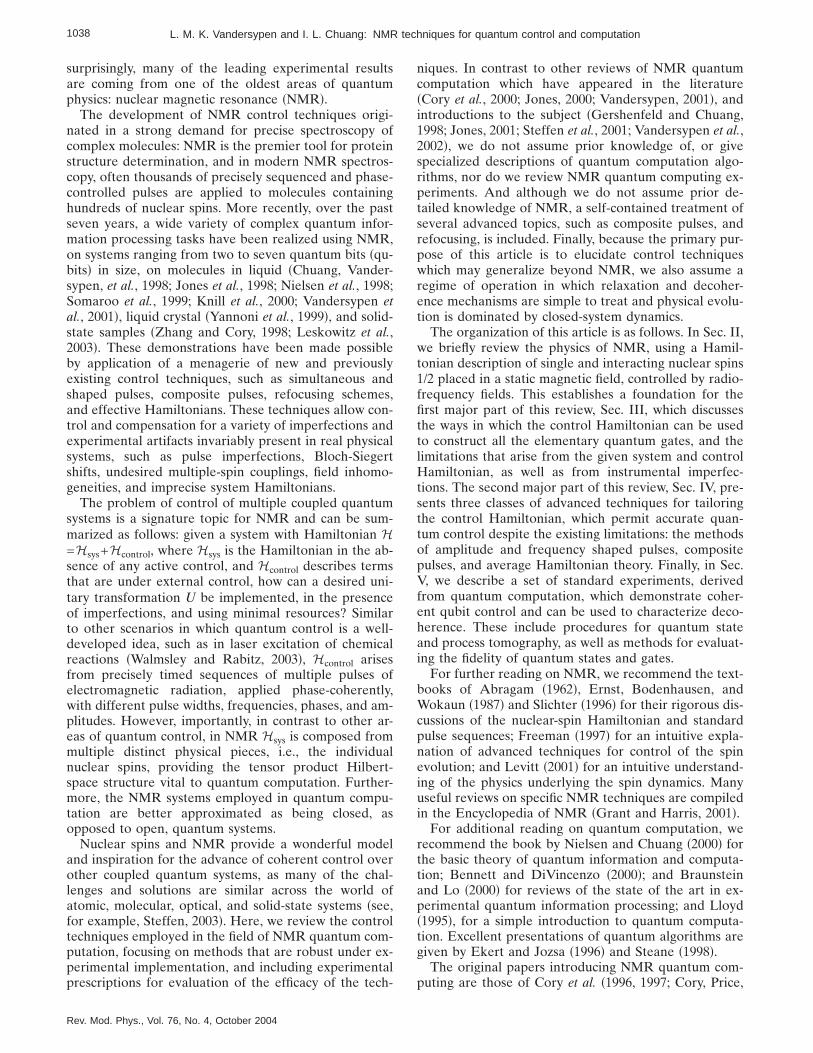
We can pictorially understand the time evolution U=e−iHt/" under the Hamiltonian of Eq. s1d as a precessing

motion of the Bloch vector about BW 0, as shown in Fig. 2.As is conventional, we define the z axis of the Blochsphere as the quantization axis of the Hamiltonian, withu0l along +z and u1l along −z.

For the case of liquid-state NMR, which we shalllargely restrict ourselves to in this article, typical valuesof B0 are 5–15 T, resulting in precession frequencies v0of a few hundred MHz, the radio-frequency range.

Spins of different nuclear species sheteronuclear spinsdcan be easily distinguished spectrally, as they have verydistinct values of g and thus also very different Larmorfrequencies sTable Id. Spins of the same nuclear speciesshomonuclear spinsd which are part of the same mol-ecule can also have distinct frequencies, by amountsknown as their chemical shifts si.

The nuclear-spin Hamiltonian for a molecule with nuncoupled nuclei is thus given by

H0 = − oi=1

n

"s1 − sidgiB0Izi = − o

i=1

n

"v0i Iz

i , s4d

where the i superscripts label the nuclei.The chemical shifts arise from partial shielding of the

externally applied magnetic field by the electron cloudsurrounding the nuclei. The amount of shielding de-pends on the electronic environment of each nucleus, solike nuclei with inequivalent electronic environmentshave different chemical shifts. Pronounced asymmetriesin the molecular structure generally promote strongchemical shifts. The range of typical chemical shifts sivaries from nucleus to nucleus, e.g., <10 parts per mil-lion sppmd for 1H, <200 ppm for 19F, and <200 ppm for13C. At B0=10 T, this corresponds to a few kHz to tensof kHz scompared to v0’s of several hundred MHzd. Asan example, Fig. 3 shows an experimentally measuredspectrum of a molecule containing five fluorine spinswith inequivalent chemical environments.

1We shall sometimes leave the factor of 2p implicit and callv0 the Larmor frequency.

FIG. 1. Energy diagram for a single spin-1 /2 particle.

FIG. 2. Precession of a spin-1 /2 particle about the axis of astatic magnetic field.

TABLE I. Larmor frequencies sMHzd for some relevant nu-clei, at 11.74 T.

Nucleus 1H 2H 13C 15N 9F 31P

v0 /2p 500 77 126 −51 470 202

1039L. M. K. Vandersypen and I. L. Chuang: NMR techniques for quantum control and computation


In general, the chemical shift can be spatially aniso-tropic and must be described by a tensor. In liquid solu-tion, this anisotropy averages out due to rapid tumblingof the molecules. In solids, the anisotropy means thatthe chemical shifts depend on the orientation of the mol-

ecule with respect to BW 0.

2. Interacting spins

For nuclear spins in molecules, nature provides twodistinct interaction mechanisms which we now describe,the direct dipole-dipole interaction, and the electron-mediated Fermi contract interaction known as J cou-pling.

a. Direct coupling

The magnetic dipole-dipole interaction is similar to theinteraction between two bar magnets in each other’s vi-cinity. It takes place purely through space—no mediumis required for this interaction—and depends on the in-ternuclear vector rWij connecting the two nuclei i and j, asdescribed by the Hamiltonian

HD = oi,j

m0gigj"

4purWiju3FIWi · IWj −

3

urWiju2sIWi · rWijdsIWj · rWijdG , s5d

where m0 is the usual magnetic permeability of free

space and IWi is the magnetic moment vector of spin i.This expression can be progressively simplified as vari-ous conditions are met. These simplifications rest on av-eraging effects and can be explained within the generalframework of average-Hamiltonian theory sSec. IV.Cd.

For large v0i =giB0 si.e., at high B0d, HD can be ap-

proximated as

HD = oi,j

m0gigj"

8purWiju3s1 – 3 cos2uijdf3Iz

i Izj − IWi · IWjg , s6d

where uij is the angle between B0 and rWij. When uv0i

−v0j u is much larger than the coupling strength, the

transverse coupling terms can be dropped, so HD simpli-fies further to

HD = oi,j

m0gigj"

4purWiju3s1 – 3 cos2uijdIz

i Izj , s7d

which has the same form as the J coupling we describenext fEq. s9dg.

For molecules in liquid solution, both intramoleculardipolar couplings sbetween spins in the same moleculedand intermolecular dipolar couplings sbetween spins indifferent moleculesd are averaged away due to rapidtumbling. This is the case we shall focus on in this ar-ticle. In solids, similarly simple Hamiltonians can be ob-tained by applying multiple-pulse sequences which aver-age out undesired coupling terms sHaeberlen andWaugh, 1968d, or by physically spinning the sample at anangle of arccoss1/Î3d sthe “magic angle”d with respect tothe magnetic field.

b. Indirect coupling

The second interaction mechanism between nuclearspins in a molecule is the J coupling or scalar coupling.This interaction is mediated by the electrons shared inthe chemical bonds between the atoms and due to theoverlap of the shared electron wave function with thetwo coupled nuclei, a Fermi contact interaction. Thethrough-bond coupling strength J depends on the respec-tive nuclear species and decreases with the number ofchemical bonds separating the nuclei. Typical values forJ are up to a few hundred Hz for one-bond couplingsand down to only a few Hz for three- or four-bond cou-plings. The Hamiltonian is

HJ = "oi,j

2pJijIWi · IWj = "o

i,j2pJijsIx

i Ixj + Iy

i Iyj + Iz

i Izj d , s8d

where Jij is the coupling strength between spins i and j.Similar to the case of dipolar coupling, Eq. s8d simplifiesto

FIG. 3. sColor in online editiond Fluorine NMR spectrum sab-solute valued centered around <470 MHz of a specially de-signed molecule, shown in sbd. The five main lines in the spec-trum correspond to the five fluorine nuclei in the molecule.The two small lines derive from impurities in the sample. TheNMR spectra were acquired by recording the oscillating mag-netic field produced by a large ensemble of precessing spinsand by taking the Fourier transform of this time-domain signal.The precession motion of the spins is started by applying aradio-frequency pulse sSec. II.B.1d, which tips the spins fromtheir equilibrium position along the z axis into the x - y plane.sbd From Vandersypen, Steffen, Breyta, Yannoni, Cleve, andChuang, 2000.



HJ = "oi,j

n

2pJijIzi Iz

j , s9d

when uvi−vju@2puJiju, a condition easily satisfied for het-eronuclear spins and which can also be satisfied for smallhomonuclear molecules.

The interpretation of the scalar coupling term of Eq.s9d is that a spin “feels” a static magnetic field along ±zproduced by the neighboring spins, in addition to the

externally applied BW 0 field. This additional field shiftsthe energy levels as in Fig. 4. As a result, the Larmorfrequency of spin i shifts by −Jij /2 if spin j is in u0l and by+Jij /2 if spin j is in u1l.

In a system of two coupled spins, the frequency spec-trum of spin i therefore actually consists of two linesseparated by Jij and centered around v0

i , each of whichcan be associated with the state of spin j, u0l or u1l. Forthree pairwise coupled spins, the spectrum of each spincontains four lines. For every additional spin, the num-ber of lines per multiplet doubles, provided all the cou-plings are resolved and different lines do not lie on topof each other. This is illustrated for a five-spin system inFig. 5.

The magnitude of all the pairwise couplings can be

found by looking for common splittings in the multipletsof different spins. The relative signs of the J couplingscan be determined via appropriate spin-selective two-pulse sequences, known in NMR as two-dimensionalcorrelation ssoft-COSYd experiments sBrüschweiler etal., 1987d or via line-selective continuous irradiation;both approaches are related to the CNOT gate sSec.III.A.3d. The signs cannot be obtained from just thesimple spectra.

In summary, the simplest form of the Hamiltonian fora system of n coupled nuclear spins is thus ffrom Eqs. s4dand s9dg

Hsys = − oi

"v0i Iz

i + "oi,j

2pJijIzi Iz

j . s10d

In almost all NMR quantum computing experimentsperformed to date, the system is well described by aHamiltonian of this form.

B. The control Hamiltonian

1. Radio-frequency fields

We turn now to physical mechanisms for controllingthe NMR system. The state of a spin-1/2 particle in a

static magnetic field BW 0 along z can be manipulated by

applying an electromagnetic field BW 1std which rotates inthe x-y plane at vrf, at or near the spin precession fre-quency v0. The single-spin Hamiltonian correspondingto the radio-frequency sRFd field is, analogous to Eq. s1dfor the static field B0,

Hrf = − "gB1fcossvrft + fdIx − sinsvrft + fdIyg , s11d

where f is the phase of the RF field, and B1 its ampli-tude sthe minus sign in front of the sine term makes theRF field evolve in the same sense as the spin evolutionunder H0d. Typical values for v1=gB1 are up to<50 kHz in liquid NMR and up to a few hundred kHz insolid NMR experiments. For n spins, we have

Hrf = − oi

n

"giB1fcossvrft + fdIxi − sinsvrft + fdIy

i g . s12d

In practice, a magnetic field is applied which oscillatesalong a fixed axis in the laboratory, perpendicular to thestatic magnetic field. This oscillating field can be decom-posed into two counter-rotating fields, one of which ro-tates at vrf in the same direction as the spin and so canbe set on or near resonance with the spin. The othercomponent rotates in the opposite direction and is thusvery far off-resonance sby about 2v0d. As we shall see,its only effect is a negligible shift in the Larmor fre-quency, called the Bloch-Siegert shift sBloch and Siegert,1940d.

Note that both the amplitude B1 and phase f of the

FIG. 4. Energy-level diagram for sdashed linesd two uncoupledspins and ssolid linesd two spins coupled by a Hamiltonian ofthe form of Eq. s7d or Eq. s9d in units of ".

FIG. 5. sColor in online editiond The spectrum of spin F1 in themolecule of Fig. 3. This is an expanded view of the left line inthe spectrum of Fig. 3. Frequencies are given with respect tov0

1. The state of the remaining spins is as indicated, based onJ12,0 and J13,J14,J15.0; furthermore, uJ12u. uJ13u. uJ15u. uJ14u.From Vandersypen, Steffen, Breyta, Yannoni, Cleve, andChuang, 2000.



RF field can be varied with time,2 unlike the Larmorprecession and the coupling terms. As we shall shortlysee, it is the control of the RF field phases, amplitudes,and frequencies which lies at the heart of quantum con-trol of NMR systems.

2. The rotating frame

The motion of a single nuclear spin subject to both astatic and a rotating magnetic field is rather complexwhen described in the usual laboratory coordinate sys-tem sthe lab framed. It is much simplified, however, bydescribing the motion in a coordinate system rotatingabout z at vrf sthe rotating framed:

uclrot = exps− ivrftIzducl . s13d

Substitution of ucl in the Schrödinger equationi"sducl /dtd=Hucl with

H = − "v0Iz − "v1fcossvrft + fdIx − sinsvrft + fdIyg

s14d

gives i"sduclrot /dtd=Hrotuclrot, where

Hrot = − "sv0 − vrfdIz − "v1fcos fIx − sin fIyg . s15d

Naturally, the RF field lies along a fixed axis in the framerotating at vrf. Furthermore, if vrf=v0, the first term inEq. s15d vanishes. In this case, an observer in the rotat-

ing frame will see the spin simply precess about BW 1 fFig.6sadg, a motion called nutation. The choice of f controlsthe nutation axis. An observer in the lab frame sees thespin spiral down over the surface of the Bloch spherefFig. 6sbdg.

If the RF field is off-resonance with respect to the spinfrequency by Dv=v0−vrf, the spin precesses in the ro-tating frame about an axis tilted away from the z axis byan angle

a = arctansv1/Dvd , s16d

and with frequency

v18 = ÎDv2 + v12, s17d

as illustrated in Fig. 7.It follows that the RF field has virtually no effect on

spins that are far off resonance, since a is very smallwhen uDvu@v1 ssee Fig. 8d. If all spins have well-separated Larmor frequencies, we can thus in principleselectively rotate any one qubit without rotating theother spins.

Moderately off-resonance pulses suDvu<v1d do rotatethe spin, but due to the tilted rotation axis, a single suchpulse cannot, for instance, flip a spin from u0l to u1l sseeagain Fig. 8d. Of course, off-resonance pulses can also beuseful, for instance, for direct implementation of rota-tions about an axis outside the x-y plane.

We could also choose to work in a frame rotating atv0 sinstead of vrfd, where

Hrot = − "v1hcosfsvrf − v0dt + fgIx

− sinfsvrf − v0dt + fgIyj . s18d

This transformation does not give a convenient time-independent RF Hamiltonian sunless vrf=v0d, as wasthe case for Hrot in Eq. s15d. However, it is a naturalstarting point for the extension to the case of multiple

2For example, the Varian Instruments Unity Inova 500 NMRspectrometer achieves a phase resolution of 0.5° and 4095 lin-ear steps of amplitude control, with a time base of 50 ns. Ad-ditional attenuation of the amplitude can be done on a loga-rithmic scale over a range of about 80 dB, albeit with a slowertime base.

FIG. 6. Nutation of a spin subject to a transverse RF field sadobserved in the rotating frame and sbd observed in the labframe.

FIG. 7. Axis of rotation sin the rotating framed during an off-resonant radio-frequency pulse.

FIG. 8. sColor in online editiond Trajectory in the Blochsphere described by a qubit initially in u0l salong +zd, after a250-ms pulse of strength v1=1 kHz is applied off-resonance by0,0.5,1 , . . . ,4 kHz. On-resonance, the pulse produces a 90° ro-tation. Far off-resonance, the qubit is hardly rotated awayfrom u0l.



spins, where a separate rotating frame can be introducedfor each spin:

uclrot = Fpi

exps− iv0i tIz

i dGucl . s19d

In the presence of multiple RF fields indexed r, the RFHamiltonian in this multiply rotating frame is

Hrot = oi,r

− "v1rhcosfsvrf

r − v0i dt + frgIx

i

− sinfsvrfr − v0

i dt + frgIyi j , s20d

where the amplitudes v1r and phases fr are under user

control.The system Hamiltonian of Eq. s10d is simplified, in

the rotating frame of Eq. s19d; the Izi terms drop out,

leaving just the JijIzi Iz

j couplings, which remain invariant.

Note that coupling terms of the form IWi ·IWj do not trans-form cleanly under Eq. s19d.

Summarizing, in the multiply rotating frame, theNMR Hamiltonian H=Hsys+Hcontrol takes the form

Hsys = "oi,j

2pJijIzi Iz

j , s21d

Hcontrol = oi,r

− "v1rhcosfsvrf

r − v0i dt + frgIx

i

− sinfsvrfr − v0

i dt + frgIyi j . s22d

C. Relaxation and decoherence

One of the strengths of nuclear spins as quantum bitsis precisely the fact that the system is very well isolatedfrom the environment, allowing coherence times to belong compared with the dynamical time scales of thesystem. Thus our discussion here focuses on closed-system dynamics, and it is important to be aware of thelimits of this approximation.

The coupling of the NMR system to the environmentmay be described by an additional Hamiltonian termHenv, whose magnitude is small compared to that of Hsysor Hcontrol. It is this coupling which leads to decoherence,the loss of quantum information, which is traditionallyparametrized by two rates: T1, the energy relaxationrate, and T2, the phase randomization rate ssee alsoSecs. V.A.4 and V.A.5d.

T2 originates from spin-spin couplings which are im-perfectly averaged away, or unaccounted for in the sys-tem Hamiltonian. For example, in molecules in liquidsolution, spins on one molecule may have a long-range,weak interaction with spins on another molecule. Fluc-tuating magnetic fields, caused by spatial anisotropy ofthe chemical shift, local paramagnetic ions, or unstablelaboratory fields, also contribute to T2. Nevertheless, inwell-prepared samples and in a good experimental appa-ratus at reasonably high magnetic fields, the T2 for mol-ecules in solution is easily on the order of 1 s or more.

This decoherence mechanism can be identified with elas-tic scattering in other physical systems; it does not leadto loss of energy from the system.

T1 originates from couplings between the spins andthe “lattice,” that is, excitation modes that can carryaway energy quanta on the scale of the Larmor fre-quency. For example, these may be vibrational quanta,paramagnetic ions, chemical reactions such as ions ex-changing with the solvent, or spins with higher-ordermagnetic moments ssuch as 2H, 17Cl, or 35Brd, which re-lax quickly due to their quadrupolar moment’s interact-ing with electric field gradients. In well-chosen mol-ecules and liquid samples with good solvents, T1 caneasily be tens of seconds, while isolated nuclei embed-ded in solid samples with a spin-zero host crystal matrixssuch as 31P in 28Sid can have T1 times of days. Thismechanism is analogous to inelastic scattering in otherphysical systems.

The description of relaxation in terms of only two pa-rameters is known to be an oversimplification of reality,particularly for coupled spin systems, in which coupledrelaxation mechanisms appear sRedfield, 1957; Jeener,1982d. Nevertheless, the independent spin decoherencemodel is useful for its simplicity and because it can cap-ture well the main effects of decoherence on simpleNMR quantum computations sVandersypen et al., 2001d,which are typically designed as pulse sequences shorterin time than T2.

III. ELEMENTARY PULSE TECHNIQUES

This section begins our discussion of the main subjectof this article, a review of the control techniques devel-oped in NMR quantum computation for coupled two-level quantum systems. We begin with a quick overviewof the language of quantum circuits and its importantuniversality theorems, then connect this with the lan-guage of pulse sequences as used in NMR, and indicatehow pulse sequences can be simplified. The main ap-proximations employed in this section are that pulsescan be strong compared with the system Hamiltonianwhile selectively addressing only one qubit at a time,and can be perfectly implemented. The limits of theseapproximations are discussed in the last part of the sec-tion.

A. Quantum control, quantum circuits, and pulses

The goal of quantum control, in the context of quan-tum computation, is the implementation of a unitarytransformation U, specified in terms of a sequence U=UkUk−1¯U2U1 of standard “quantum gates” Ui, whichact locally susually on one or two qubitsd and are simpleto implement. As is conventional for unitary operations,the Ui are ordered in time from right to left.

1. Quantum gates and circuits

The basic single-qubit quantum gates are rotations,defined as



Rnsud = expF−iun · sW

2G , s23d

where n is a sthree-dimensionald vector specifying theaxis of the rotation, u is the angle of rotation, and sW=sxx+syy+szz is a vector of Pauli matrices. It is alsoconvenient to define the Pauli matrices fsee Eq. s3dgthemselves as logic gates, in terms of which sx can beunderstood as being analogous to the classical NOT gate,which flips u0l to u1l and vice versa. In addition, theHADAMARD gate H and p /8 gate T

H =1Î2F1 1

1 − 1G, T = F1 0

0 expsip/4d G s24d

are useful and widely employed. These and any othersingle-qubit transformation U can be realized using asequence of rotations about just two axes, according toBloch’s theorem: for any single-qubit U, there exist realnumbers a , b , g, and d such that

U = eiaRxsbdRysgdRxsdd . s25d

The basic two-qubit quantum gate is a controlled-NOTsCNOTd gate,

UCNOT = 31 0 0 0

0 1 0 0

0 0 0 1

0 0 1 04 , s26d

where the basis elements in this notation are u00l, u01l,u10l, and u11l from left to right and top to bottom. UCNOTflips the second qubit sthe targetd if and only if the firstqubit sthe controld is u1l. This gate is the analog of theclassical exclusive-OR gate, since UCNOTux ,yl= ux ,x % yl,for x ,yP h0,1j and where % denotes addition modulotwo.

A basic theorem of quantum computation is that up toan irrelevant overall phase, any U acting on n qubits canbe composed from UCNOT and Rnsud gates sNielsen andChuang, 2000d. Thus the problem of quantum controlcan be reduced to implementing UCNOT and single-qubitrotations, where at least two nontrivial rotations are re-quired. Other such sets of universal gates are known, butthis is the one that has been employed in NMR.

These gates and sequences of such gates may be con-veniently represented using quantum circuit diagrams,employing standard symbols. We shall use a notationcommonly employed in the literature sNielsen andChuang, 2000d in this article.

2. Implementation of single-qubit gates

Rotations on single qubits may be implemented di-rectly in the rotating frame using RF pulses. From thecontrol Hamiltonian, Eq. s22d, it follows that when anRF field of amplitude v1 is applied to a single-spin sys-tem at vrf=v0

, the spin evolves under the transformation

U = expfiv1scos fIx − sin fIydtpwg , s27d

where tpw is the pulse width sor pulse lengthd, the timeduration of the RF pulse. U describes a rotation in theBloch sphere over an angle u proportional to the prod-uct of tpw and v1=gB1, and about an axis in the x-yplane determined by the phase f.

Thus a pulse with phase f=p and v1tpw=p /2 will per-form Rxs90d fsee Eq. s23dg, which is a 90° rotation aboutx, denoted for short as X. A similar pulse but twice aslong realizes a Rxs180d rotation, written for short as X2.By changing the phase of the RF pulse to f=p /2, Y andY2 pulses can similarly be implemented. For f=0, a

negative rotation about x, denoted Rxs−90d or X, is ob-

tained, and similarly f=−p /2 gives Y. For multiqubitsystems, subscripts are used to indicate on which qubit

the operation acts, e.g., Z32 is a 180° rotation of qubit 3

about −z.It is thus not necessary to apply the RF field along

different spatial axes in the lab frame to perform x and yrotations. Rather, the phase of the RF field determinesthe nutation axis in the rotating frame. Furthermore,note that only the relative phase between pulses appliedto the same spin matters. The absolute phase of the firstpulse on any given spin does not matter in itself. It justestablishes a phase reference against which the phases ofall subsequent pulses on that same spin, as well as theread-out of that spin, should be compared.

We noted earlier that the ability to implement arbi-trary rotations about x and y is sufficient for performingarbitrary single-qubit rotations fEq. s25dg. Since z rota-tions are very common, two useful explicit decomposi-tions of Rzsud in terms of x and y rotations are

Rzsud = XRysudX = YRxs− udY . s28d

3. Implementation of two-qubit gates

The most natural two-qubit gate is the one generateddirectly by the spin-spin coupling Hamiltonian. Fornuclear spins in a molecule in liquid solution, the cou-pling Hamiltonian is given by Eq. s9d sin the lab frame aswell as in the rotating framed, from which we obtain thetime evolution operator UJstd=expf−i2pJIz

1Iz2tg, or in

matrix form

UJstd = 3e−ipJt/2 0 0 0

0 e+ipJt/2 0 0

0 0 e+ipJt/2 0

0 0 0 e−ipJt/24 . s29d

Allowing this evolution to occur for time t=1/2J gives atransformation known as the controlled phase gate, up toa 90° phase shift on each qubit and an overall sand thusirrelevantd phase

UCPHASE = Î− iZ1Z2UJs1/2Jd = 31 0 0 0

0 1 0 0

0 0 1 0

0 0 0 − 14 . s30d



This gate is equivalent to the well-known CNOT gate upto a basis change of the target qubit and a phase shift onthe control qubit

UCNOT = iZ12Y2UCPHASEY2

= iZ12Y2fÎ− iZ1Z2UJs1/2JdgY2

= ÎiZ1Z2X2UJs1/2JdY2 = 31 0 0 0

0 1 0 0

0 0 0 1

0 0 1 04 . s31d

The core of this sequence, X2UJs1/2JdY2, can be graphi-cally understood via Fig. 9 sGershenfeld and Chuang,1997d, assuming the spins start along ±z. First, a spin-selective pulse on spin 2 about y san rf pulse centered atv0

2 /2p and of a spectral bandwidth such that it coversthe frequency range v0

2 /2p±J12/2 but not v01 /2p±J12/2d

rotates spin 2 from z to x. Next, the spin system is al-lowed to freely evolve for a duration of 1/2J12 seconds.Because the precession frequency of spin 2 is shifted by±J12/2 depending on whether spin 1 is in u1l or u0l sseeFig. 4d, spin 2 will arrive in 1/2J seconds at either +y or−y, depending on the state of spin 1. Finally, a 90° pulseon spin 2 about the x axis rotates spin 2 back to +z ifspin 1 is u0l, or to −z if spin 1 is in u1l.

The net result is that spin 2 is flipped if and only ifspin 1 is in u1l, which corresponds exactly to the classicaltruth table for the CNOT. The extra z rotations in Eq.s31d are needed to give all elements in UCNOT the samephase, so the sequence works also for superposition in-put states.

An alternative implementation of the CNOT gate, upto a relative phase factor, consists of applying a line-selective 180° pulse at v0

2+J12/2 ssee Fig. 4d. This pulseinverts spin 2 sthe target qubitd if and only if spin 1 sthecontrold is u1l sCory, Price, and Havel, 1998d. In general,if a spin is coupled to more than one other spin, half thelines in the multiplet must be selectively inverted in or-der to realize a CNOT. Extensions to doubly controlledNOT’s are straightforward: in a three-qubit system, forexample, this can be realized through inversion of oneout of the eight lines sFreeman, 1998d. As long as all thelines are resolved, it is in principle possible to invert anysubset of the lines. Demonstrations using very long mul-tifrequency pulses have been performed with up to fivequbits sKhitrin et al., 2002d. However, this approach can-

not be used whenever the relevant lines in the multipletfall on top of each other.

If the spin-spin interaction Hamiltonian is not of theform Iz

i Izj but contains also transverse components fas in

Eqs. s5d, s6d, and s8dg, other sequences of pulses areneeded to perform the CPHASE and CNOT gates. Thesesequences are somewhat more complicated sBremner etal., 2002d.

If two spins are not directly coupled to each other, it isstill possible to perform a CNOT gate between them, aslong as there exists a network of couplings that connectsthe two qubits. For example, suppose we want to per-form a CNOT gate with qubit 1 as the control and qubit 3as the target, CNOT13, but 1 and 3 are not coupled to eachother. If both are coupled to qubit 2, as in the couplingnetwork of Fig. 10sbd, we can first swap the states ofqubits 1 and 2 svia the sequence CNOT12 CNOT21 CNOT12d,then perform a CNOT23, and finally swap qubits 1 and 2again sor relabel the qubits without swapping backd. Thenet effect is CNOT13. By extension, at most Osnd SWAPoperations are required to perform a CNOT between anypair of qubits in a chain of n spins with just nearest-neighbor couplings fFig. 10sbdg. SWAP operations canalso be used to perform two-qubit gates between anytwo qubits that are coupled to a common “bus” qubitfFig. 10scdg.

Conversely, if a qubit is coupled to many other qubitsfFig. 10sadg and we want to perform a CNOT between justtwo of them, we must remove the effect of the remainingcouplings. This can accomplished using the technique ofrefocusing, which has been widely adopted in a varietyof NMR experiments.

4. Refocusing: Turning off undesired Izi Iz

j couplings

The effect of coupling terms during a time interval offree evolution can be removed via so-called “refocusing”techniques. For coupling Hamiltonians of the form Iz

i Izj ,

as is often the case in liquid NMR experiments fsee Eq.s9dg, the refocusing mechanism can be understood at avery intuitive level. Reversal of the effect of couplingHamiltonians of other forms, such as in Eqs. s5d, s6d, ands8d, is less intuitive, but can be understood within the

FIG. 9. Bloch-sphere representation of the operation of theCNOT12 gate between two qubits 1 and 2 coupled by "2pJIz

1Iz2.

Here, qubit 2 starts off in u0l salong zd and is depicted in areference frame rotating about z at v0

2 /2p. Solid and dashedarrows correspond to the case where qubit 1 is u0l and u1l,respectively. Adapted from Gershenfeld and Chuang, 1997.

FIG. 10. Three possible coupling networks between fivequbits. sad A full coupling network. Such networks will in prac-tice always be limited in size, as physical interactions tend todecrease with distance. sbd A nearest-neighbor coupling net-work. Such linear chains with nearest-neighbor couplings ortwo-dimensional variants are used in many solid-state propos-als. scd Coupling via a “bus.” This network is used in ion-trapschemes, for example. As in case sad, the bus degreeof freedom will in reality couple well to only a finite number ofqubits.



framework of average Hamiltonian theory sSec. IV.Cd.Let us first look at two ways of undoing Iz

i Izj in a two-

qubit system. In Fig. 11sad, the evolution of qubit 1 inthe first time interval t is reversed in the second timeinterval, due to the 180° pulse on qubit 2. In Fig. 11sbd,qubit 1 continues to evolve in the same direction all thetime, but the first 180° pulse causes the two componentsof qubit 1 to be refocused by the end of the second timeinterval. The second 180° pulse ensures that both qubitsalways return to their initial state.

Mathematically, we can see how refocusing of J cou-plings works using the fact that for all t

X12UJstdX1

2 = UJs− td = X22UJstdX2

2, s32d

which leads to

X12UJstdX1

2UJstd = I = X22UJstdX2

2UJstd . s33d

Replacing all Xi2 with Yi

2, the sequence works just thesame. However, if we sometimes use Xi

2 and sometimesYi

2, we get the identity matrix only up to some phaseshifts. Also, if we applied pulses on both qubits simulta-neously, e.g., X1

2X22 UJstdX1

2X22 UJstd, the coupling would

not be removed.Figure 12 gives insight into refocusing techniques in a

multiqubit system. Specifically, this scheme preserves theeffect of J12, while effectively inactivating all the othercouplings. The underlying idea is that a coupling be-tween spins i and j acts “forward” during intervals whereboth spins have the same sign in the diagram, and acts

“in reverse” whenever the spins have opposite signs.Whenever a coupling acts forward and in reverse for thesame duration, it has no net effect.

Systematic methods for designing refocusing schemesfor multiqubit systems have been developed specificallyfor the purpose of quantum computing. The most com-pact scheme is based on Hadamard matrices sJones andKnill, 1999; Leung et al., 2000d. A Hadamard matrix oforder n, denoted by Hsnd, is an n3n matrix with entries±1 such that

HsndHsndT = nI . s34d

The rows are thus pairwise orthogonal, and any tworows agree in exactly half of the entries. Identifying +1and −1 with + and − as in the diagram of Fig. 12, we seethat Hsnd gives a valid decoupling scheme for n spinsusing only n time intervals. An example of Hs12d is

3+ + + + + + + + + + + +

+ + + − − + − − + − − +

+ + + + − − − + − + − −

+ − + + + − − − + − + −

+ − − + + + − − − + − +

+ + − − + + − + − − + −

+ − − − − − − + + + + +

+ − + − − + + − − + + −

+ + − + − − + − − − + +

+ − + − + − + + − − − +

+ − − + − + + + + − − −

+ + − − + − + − + + − −

4 . s35d

If we want the coupling between one pair of qubits toremain active while removing the effect of all other cou-plings, we can simply use the same row of Hsnd for thosetwo qubits.

Hsnd does not exist for all n, but we can always find adecoupling sequence for n qubits by taking the first nrows of Hsnd, with n the smallest integer that satisfiesnùn with known Hsnd. From the properties of Had-amard matrices, we can show that n /n is always close to1 sLeung et al., 2000d. So decoupling schemes for n spinsrequire n time intervals and no more than nn 180°pulses.

Another systematic approach to refocusing sequencesis illustrated via the following four-qubit scheme sLin-den, Barjat, et al., 1999d:

3+ + + + + + + +

+ + + + − − − −

+ + − − − − + +

+ − − + + − − +4 . s36d

For every additional qubit, the number of time intervalsis doubled, and 180° pulses are applied to this qubit afterthe first, third, fifth, . . . time interval. The advantage ofthis scheme over schemes based on Hadamard matrices

FIG. 11. Bloch-sphere representation of the operation of twosimple schemes to refocus the coupling between two coupledqubits. The diagram shows the evolution of qubit 1 sin therotating framed initially along −y, when qubit 2 is in u0l ssoliddor in u1l sdashedd. The refocusing pulse can be applied to eithersad qubit 2 or sbd qubit 1.

FIG. 12. Refocusing scheme for a four-spin system, designedto leave J12 active the whole time but to neutralize the effect ofthe other Jij. The interval is divided into slices of equal dura-tion, and the “+” and “−” signs indicate whether a spin is stillin its original position, or upside down. The black rectanglesrepresent 180° pulses, which flip the corresponding spin.



is that it does not require simultaneous rotations of mul-tiple qubits. The main drawback is that the number oftime intervals increases exponentially.

We end this subsection with three additional remarks.First, each qubit will generally be coupled to no morethan a fixed number of other qubits, since couplingstrengths tend to decrease with distance. In this case, allrefocusing schemes can be greatly simplified sJones andKnill, 1999; Linden, Barjat, et al., 1999; Leung et al.,2000d.

Second, if the forward and reverse evolutions under Jijare not equal in duration, a net coupled evolution takesplace corresponding to the excess forward or reverseevolution. In principle, therefore, we can organize anyrefocusing scheme such that it incorporates any desiredamount of coupled evolution for each pair of qubits.

Third, refocusing sequences can also be used to re-move the effect of Iz

i terms in the Hamiltonian. Ofcourse, these terms vanish in principle if we work in themultiply rotating frame fsee Eq. s21dg. However, theremay be some spread in the Larmor frequencies, for in-stance, due to magnetic-field inhomogeneities. This ef-fect can then be reversed using refocusing pulses, as isroutinely accomplished in spin-echo experiments sSec.V.A.4d.

5. Pulse sequence simplification

There are many possible pulse sequences which in anideal world result in exactly the same unitary transfor-mation. Good pulse sequence design therefore attemptsto find the shortest and most effective pulse sequencethat implements the desired transformations. In Sec. IV,we shall see that the use of more complex pulses or

pulse sequences may sometimes increase the degree ofquantum control. Here, we look at three levels of pulsesequence simplification.

At the most abstract level of pulse sequence simplifi-cation, careful study of a quantum algorithm can giveinsight into how to reduce the resources needed. Forexample, a key step in both the modified Deutsch-Jozsaalgorithm sCleve et al., 1998d and the Grover algorithmsGrover, 1997d can be described as the transformationuxluyl→ uxlux % yl, where uyl is set to su0l− u1ld /Î2, sothat the transformation in effect is uxlsu0l− u1ld /Î2→ s−1dfsxduxlsu0l− u1ld /Î2. Thus we might as well leaveout the last qubit as it is never changed.

At the next level, that of quantum circuits, we can usesimplification rules such as those illustrated in Fig. 13. Inthis process, we can fully take advantage of commuta-tion rules to move building blocks around, as illustratedin Fig. 14. Furthermore, gates that commute with eachother can be executed simultaneously. Finally, we cantake advantage of the fact that most building blockshave many equivalent implementations, as shown, forinstance, in Fig. 15.

Sometimes, a quantum gate may be replaced by an-other quantum gate, which is easier to implement. Forinstance, refocusing sequences sSec. III.A.4d can be keptsimple by examining which couplings really need to berefocused. Early on in a pulse sequence, several qubitsmay still be along ±z, in which case their mutual Iz

i Izj

couplings have no effect and thus need not be refocused.Similarly, if a subset of the qubits can be traced out atsome point in the sequence, the mutual interaction be-tween these qubits does not matter anymore, so onlytheir coupling with the remaining qubits must be refo-cused. Figure 16 gives an example of such a simplifiedrefocusing scheme for five coupled spins.

FIG. 13. Simplification rules for quantum circuits, drawn usingstandard quantum gate symbols, where time goes from left toright, each wire represents a qubit, boxes represent simplegates, and solid black dots indicate control terminals.

FIG. 14. Commutation of unitary operators can help simplifyquantum circuits by moving building blocks around such thatcancellation of operations as in Fig. 13 becomes possible. Forexample, the three segments sseparated by dashed linesd inthese two equivalent realizations of the TOFFOLI gate sdoubly-controlled NOTd commute with each other and can thus be ex-ecuted in any order.

FIG. 15. Choosing one of several equivalent implementationscan help simplify quantum circuits, again by enabling cancella-tion of operations as in Fig. 13. For instance, the two controlqubits in the TOFFOLI gate play equivalent roles, so they can beinterchanged.

FIG. 16. Simplified refocusing scheme for five spins, designedsuch that the coupling of qubits 1-2 with qubits 3-5 is switchedoff, i.e., J13, J14, J15, J23, J24, and J25 are inactive whereasJ12, J34, J35, and J45 are active.



More generally, the relative phases between the en-tries in the unitary matrix describing a quantum gate areirrelevant when the gate acts on a diagonal density ma-trix. In this case, we can, for instance, implement a CNOT

simply as X2UJs1/2JdY2 rather than the sequence ofEq. s31d.

At the lowest level, that of pulses and delay times,further simplification is possible by taking out adjacent

pulses which cancel out, such as X and X san instance ofthe first simplification rule of Fig. 13d and by converting“difficult” operations to “easy” operations.

Cancellation of adjacent pulses can be maximized byproperly choosing the pulse sequences for subsequentquantum gates. For this purpose, it is convenient to havea library of equivalent implementations for the mostcommonly used quantum gates. For example, twoequivalent decompositions of a CNOT12 gate swith J12.0d are

Z1Z2X2UJS 1

2JDY2, s37d

as in Eq. s31d, and

Z1Z2X2UJS 1

2JDY2. s38d

Similarly, two equivalent implementations of theHADAMARD gate on qubit 2 are

X22Y2 s39d

and

Y2X22. s40d

Thus, if we need to perform a HADAMARD operation onqubit 2 followed by a CNOT12 gate, it is best to choose thedecompositions of Eqs. s37d and s40d, such that the re-sulting pulse sequence,

Z1Z2X2UJS 1

2JD Y2 Y2X2

2, s41d

simplifies to

Z1Z2X2UJS 1

2JD X2

2. s42d

An example of a set of operations that is easy to per-form is the rotations about z. While the implementationof z rotations in the form of three RF pulses fEq. s28dgtakes more work than a rotation about x or y, rotationsabout z need in fact not be executed at all, provided thecoupling Hamiltonian is of the form Iz

i Izj , as in Eq. s21d.

In this case, z rotations commute with free evolutionunder the system Hamiltonian, so we can interchangethe order of z rotations and time intervals of free evo-lution. Using equalities such as

ZY = XYXY = XZ , s43d

we can also move z rotations across x and y rotations,and gather all z rotations at the end or the beginning of

a pulse sequence. At the end, z rotations do not affectthe outcome of measurements in the usual u0l, u1l “com-putational” basis. Similarly, z rotations at the start of apulse sequence have no effect on the usually diagonalinitial state. In either case, Z rotations do not then re-quire any physical pulses and are in a sense “for free”and perfectly executed. Indeed, Z rotations simply de-fine the reference frame for x and y and can be imple-mented by changing the phase of the reference framethroughout the pulse sequence.

It is thus advantageous to convert as many X and Yrotations as possible into Z rotations, using identitiessimilar to Eq. s28d, for example,

XY = XYXX = ZX . s44d

A key point in pulse sequence simplification of anykind is that the simplification process must itself be effi-cient. For example, suppose an algorithm acts on fivequbits with initial state u00000l and outputs the finalstate su01000l+ u01100l /Î2. The overall result of the al-gorithm is thus that qubit 2 is flipped and that qubit 3 isplaced in an equal superposition of u0l and u1l. This nettransformation can obviously be obtained immediatelyby the sequence X2

2Y3. However, the effort needed tocompute the overall input-output transformation gener-ally increases exponentially with the problem size, sosuch extreme simplifications are not practical.

6. Time-optimal pulse sequences

Next to the widely used but rather naive set of pulsesequence simplification rules of the previous subsection,there exist powerful mathematical techniques for de-terming the minimum time needed to implement aquantum gate, using a given system and control Hamil-tonian, as well as for finding time-optimal pulse se-quences sKhaneja et al., 2001d. These methods build onearlier optimization procedures for mapping an initialoperator onto a final operator via unitary transforma-tions sSørenson, 1989; Glaser et al., 1998d, as in coher-ence or polarization transfer experiments, common tasksin NMR spectroscopy.

The pulse sequence optimization technique expressespulse sequence design as a geometric problem in thespace of all possible unitary transformations. The goal isto find the shortest path between the identity transfor-mation I and the point in the space corresponding to thedesired quantum gate, U, while traveling only in direc-tions allowed by the given system and control Hamil-tonian. Let us call K the set of all unitaries k that can beproduced using the control Hamiltonian only. Next weassume that the terms in the control Hamiltonian aremuch stronger than the system Hamiltonian sas we shallsee in Sec. III.B.2, this assumption is valid in NMR onlywhen using so-called hard, high-power pulsesd. Then,starting from I, any point in K can be reached in a neg-ligibly short time, and similarly, U can be reached in notime from any point in the coset KU, defined by hkUukPKj. Evolution under the system Hamiltonian for a fi-



nite amount of time is required to reach the coset KUstarting from K. Finding a time-optimal sequence for Uthus comes down to finding the shortest path from K toKU allowed by the system Hamiltonian.

Such optimization problems have been extensivelystudied in mathematics sBrockett, 1981d and have beensolved explicitly for elementary quantum gates on twocoupled spins sKhaneja et al., 2001d and a three-spinchain with nearest-neighbor couplings sKhaneja et al.,2002d. For example, a sequence was found for producingthe trilinear propagator exps−i2pIz

1Iz2Iz

3d from the systemHamiltonian "2pJsIz

1Iz2+Iz

2Iz3d in a time Î3/2J, the short-

est possible time sKhaneja et al., 2002d. This propagatoris the starting point for useful quantum gates such as thedoubly controlled NOT or TOFFOLI gate. The standardquantum circuit approach, in comparison, would yield asequence of duration 3/2J sit uses only one coupling at atime while refocusing the other couplingd, and the com-mon NMR pulse sequence has duration 1/J.

Clearly, the time needed to find a time-optimal pulsesequence increases exponentially with the number of qu-bits n involved in the transformation, since the unitarymatrices involved are of size 2n32n. Therefore the mainuse of the techniques presented here lies in finding effi-cient pulse sequences for building blocks acting on onlya few qubits at a time, which can then be incorporated inmore complex sequences acting on many qubits by add-ing appropriate refocusing pulses to remove the cou-plings with the remaining qubits. While the examplesgiven here are for the typical NMR system and controlHamiltonian, the approach is completely general andmay be useful for other qubit systems too.

B. Experimental limitations

Many years of experience have taught NMR spectros-copists that while the ideal control techniques describedabove are theoretically attractive, they neglect impor-tant experimental artifacts and undesired Hamiltonianterms which must be addressed in any actual implemen-tation. First, a pulse intended to selectively rotate onespin will to some extent also affect the other spins. Sec-ond, the coupling terms 2pJijIz

i Izj cannot be switched off

in NMR. During time intervals of free evolution underthe system Hamiltonian, the effect of these couplingterms can easily be removed using refocusing techniquessSec. III.A.4d, so long as the single-qubit rotations areperfect and instantaneous. However, during RF pulsesof finite duration, the coupling terms also distort thesingle-qubit rotations. In addition to these two limita-tions arising from the NMR system and control Hamil-tonian, a number of instrumental imperfections causeadditional deviations from the intended transformations.

1. Cross-talk

Throughout the discussion of single- and two-qubitgates, we have assumed that we can selectively addresseach qubit. Experimentally, qubit selectivity could be ac-complished if the qubits were well separated in space or,

as in NMR, in frequency. In practice, there will usuallybe some cross-talk, which causes an RF pulse applied onresonance with one qubit to slightly rotate another qubitor shift its phase. Cross-talk effects are even more com-plex when two or more pulses are applied simulta-neously.

The frequency bandwidth over which qubits are ro-tated by a pulse of length tpw is roughly speaking oforder 1/ tpw. Yet, since the qubit response to an RF fieldis not linear sit is sinusoidal in v1tpwd, the exact fre-quency response cannot be computed using Fouriertheory.

For a constant-amplitude srectangulard pulse, the uni-tary transformation as a function of the detuning Dv iseasy to derive analytically from Eqs. s16d and s17d. Al-ternatively, we can exponentiate the Hamiltonian of Eq.s15d to get U directly. An example of a qubit response toa rectangular pulse is shown in Fig. 17.

It is evident from Fig. 17 that short rectangular pulsessknown as “hard” pulsesd excite spins over a very widefrequency range. The frequency selectivity of a pulse canof course be increased by increasing tpw while loweringB1 accordingly sthus creating what is known as a “soft”pulsed, but decoherence effects become more severe asthe pulses get longer. Fortunately, as we shall see in Secs.IV.A and IV.B, the use of shaped and composite pulsescan dramatically improve the frequency selectivity of theRF excitation.

Even if a pulse is designed not to produce any net x ory rotations of spins outside a specified frequency win-dow, the presence of RF irradiation during the pulse stillcauses a shift DvBS

i in the precession frequency of spinsi at frequencies well outside the excitation frequencywindow sEmsley and Bodenhausen, 1990d. As a result,each spin accumulates a spurious phase shift during RFpulses applied to spins at nearby frequencies.

This effect is related to the Bloch-Siegert shift men-tioned in Sec. II.B.1 and is known as the transient gener-alized Bloch-Siegert shift in the NMR community. It isrelated to the ac Stark effect in atomic physics. At adeeper level, the acquired phase can be understood as

FIG. 17. Simulation of the spin response to a 1-ms constant-amplitude RF pulse as a function of the frequency offset Dvbetween v0 and vrf. The spin starts off in u0l salong +z in theBloch sphered and v1 /2p=500 Hz is chosen such that the ro-tation angle amounts to 180° for an on-resonance pulse.



an instance of Berry’s phase sBerry, 1984d: the spin de-scribes a closed trajectory on the surface of the Blochsphere and thus returns to its initial position, but it ac-quires a phase shift proportional to the area enclosed byits trajectory.

The frequency shift is given by

DvBS <v1

2

2sv0 − vrfds45d

sprovided v1! uv0−vrfud, where v0 /2p is the originalLarmor frequency sin the absence of the RF fieldd. Intypical NMR experiments, the frequency shifts can eas-ily reach several hundred Hz in magnitude. We see fromEq. s45d that the Larmor frequency shifts up if v0.vrfand shifts down if v0,vrf.

Fortunately, the resulting phase shifts can be easilycomputed in advance for each possible spin-pulse com-bination, if all the frequency separations, pulse ampli-tude profiles, and pulse lengths are known. The unin-tended phase shifts Rzsud can then be compensated forduring the execution of a pulse sequence by insertingappropriate Rzs−ud, which can be executed at no cost, aswe saw in Sec. III.A.5.

Cross-talk effects are aggravated during simultaneouspulses, applied to two or more spins with nearby fre-quencies v0

1 and v02 ssay v0

1,v02d. The pulse at v0

1 thentemporarily shifts the frequency of spin 2 to v0

2+DvBS.As a result, the pulse on spin 2, if applied at v0

2, will beoff-resonance by an amount −DvBS. Analogously, thepulse at v0

1 is now off the resonance of spin 1 by DvBS.The resulting rotations of the spins deviate significantlyfrom the intended rotations.

The detrimental effect of the Bloch Siegert shifts dur-ing simultaneous pulses is illustrated in Fig. 18, whichshows the simulated inversion profile for a spin subjectto two simultaneous 180° pulses separated by 3273 Hz.The centers of the inverted regions have shifted awayfrom the intended frequencies and the inversion is in-

complete, which can be seen most clearly from the sub-stantial residual x–y-magnetization s.30%d over thewhole region intended to be inverted. Note also thatsince the frequencies of the applied pulses are off thespin resonance frequencies, complete inversion cannotbe achieved no matter what tip angle is chosen ssee Sec.II.B.2d.

In practice, simultaneous soft pulses at nearby fre-quencies have been avoided in NMR sLinden, Kup~e,and Freeman, 1999d or the poor quality of the spin rota-tions was accepted. Pushed by the stringent require-ments of quantum computation, several techniques havemeanwhile been invented to generate accurate simulta-neous rotations of spins at nearby frequencies ssee Secs.IV.A.2 and IV.B.2d.

2. Coupled evolution

The spin-spin couplings in a molecule are essential forthe implementation of two-qubit gates sSec. III.A.3d, butthey cannot be turned off and are thus also active duringthe RF pulses, which are intended to be just single-qubittransformations. Unless v1 is much stronger than thecoupling strength, the interactions strongly affect the in-tended nutation. For couplings of the form JIz

i Izj , the

effect is similar to the off-resonance effects illustrated inFig. 7: the coupling to another spin shifts the spin fre-quency to v0 /2p±J /2, so a pulse sent at v0 /2p hits thespin off-resonance by 7J /2.

In practice, J coupling terms can only be neglected forshort, high-power pulses used in heteronuclear spin sys-tems: typically J,300 Hz while v1 is up to <50 kHz.For low-power pulses, often used in homonuclear spinsystems, v1 can be of the same order as J and couplingeffects become prominent. The coupling terms also leadto additional complications when two qubits are pulsedsimultaneously. In general, the qubits become partiallyentangled sKup~e and Freeman, 1995d.

As was the case for cross-talk, NMR spectroscopistshave developed special shaped and composite pulses tocompensate for coupling effects during RF pulses whileperforming spin-selective rotations. In recent years, theuse of such pulses has been extended and perfected forquantum computing experiments sSecs. IV.A and IV.Bd.

3. Instrumental errors

A number of experimental imperfections lead to er-rors in the quantum gates. In NMR, the most commonimperfections are inhomogeneities in the static and RFmagnetic field, pulse length calibration errors, frequencyoffsets, and pulse timing and phase imperfections.

The static field B0 in modern NMR magnets can bemade homogeneous over the sample volume sa cylinder5 mm in diameter and 1.5 cm longd to better than 1 partin 109. This amazing homogeneity is obtained by meticu-lously adjusting the current through a set of so-called“shim” coils, which compensate for the inhomogeneitiesproduced by the large solenoid. At v0=500·2p MHz,linewidths of 0.5 Hz can thus be obtained, correspond-

FIG. 18. Simulation of the spin response to two simultaneouspulses with carrier frequencies at 0 Hz and 3273 Hz sverticaldashed linesd away from the spin-resonance frequency, with acalibrated pulse length of 2650 ms sas for an ideal 180°d. Theamplitude profile of the pulses is Hermite shaped sSec. IV.Adin order to obtain a smooth spin response. For ideal inversion,the solid line should be −1 at the two frequencies, and thedashed line should be zero. From Steffen et al., 2000.



ing to a dephasing time constant T2* ssee Sec. V.A.2d of

1/ s2p0.5d=0.32 s. In the course of long pulse sequencessof order 0.1–1 sd, even the tiny remaining inhomogene-ity would therefore have a large effect, so its effect mustbe reversed using refocusing sequences sSec. III.A.4d

The RF field homogeneity is typically very poor, dueto constraints on the geometry of the RF coils: the en-velope of Rabi oscillations sSec. V.A.1d often decays byas much as 5% per 90° rotation, corresponding to aquality factor of only <5. In sequences containing only afew pulses, this is not problematic, but in multiple-pulseexperiments, the RF field inhomogeneity is often thedominant source of errors and signal loss.

Imperfect pulse length calibration has an effect similarto B1 inhomogeneity: the qubit rotation angle is differ-ent than was intended. Only the correlation time for theerror is different. Miscalibrations are constant through-out an experiment, whereas the RF field experienced byany given molecule changes on the time scale of diffu-sion through the sample volume.

Frequency offsets occur in different contexts. In tradi-tional NMR experiments, the Larmor frequencies areoften not known in advance. RF pulses are then ex-pected to rotate the spins over a wide range of frequen-cies, quite the opposite case to that of quantum comput-ing, where the Larmor frequencies are precisely knownand rotations should be spin selective. However, wehave seen earlier that Iz

i Izj coupling terms act as a fre-

quency offset of one spin, which depends on the state ofthe other spin. Qubit-selective rotations of qubit i thusrequire a uniform rotation over a range v0

i ±ojÞi uJiju /2.Various approaches have been developed to reduce

the sensitivity of RF pulses and pulse sequences to theseinstrumental errors, sometimes in combination with so-lutions to cross-talk and coupling artifacts. These ad-vanced techniques are the subject of the next section.

IV. ADVANCED PULSE TECHNIQUES

The accuracy of quantum gates that can be achievedusing the simple pulse techniques of the previous sectionis unsatisfactory when applied to multispin systems,where the given NMR system and control Hamiltonianlead to undesired cross-talk and coupling effects. In ad-dition, the available instrumentation can only imper-fectly approximate ideal pulse amplitudes, timings, andphases, for realistic sample geometries and coil configu-rations, and any real molecule includes additionalHamiltonian terms such as couplings to the environ-ment, which are undesired. Nevertheless, extremely pre-cise control can be achieved despite these imperfections,and this is accomplished using the art of shaped pulses,composite pulses, and average Hamiltonian theory, thesubject of this second major section of this review.

These advanced techniques are based on the assump-tion that errors are, at least on some accessible timescale, systematic, rather than random. This assumptionclearly holds for the terms in the ideal NMR Hamil-tonian of Eqs. s21d and s22d, and applies also to most

instrumental errors. Then, by using the special proper-ties of evolution in unitary groups, such as the SUs2ndwhich describes the space of operators acting on n qu-bits, the systematic errors can in principle be canceledout.

A. Shaped pulses

The amplitude and phase profile of RF pulses can bespecially tailored in order to ease the cross-talk and cou-pling effects discussed in Secs. III.B.1 and III.B.2. Inpractice, the pulse is divided into a few tens to manyhundreds of discrete time slices; to achieve an arbitrarilyshaped pulse, it suffices to control the amplitude andphase of the slices separately. Furthermore, multipleshaped pulses applied at various frequencies can becombined into a single pulse shape, since a linear vectorsum of pulse slices also results in a valid pulse. Here, weconsider simple amplitude and phase shaped pulses.

1. Amplitude profiles

The frequency selectivity of RF pulses can be muchimproved compared to standard rectangular pulses withsharp edges, by using pulse shapes that smoothly modu-late the pulse amplitude with time. Such pulses are typi-cally especially designed to excite or invert spins over alimited frequency region, while minimizing x and y ro-tations for spins outside this region sFreeman, 1997,1998d.

Furthermore, specialized pulse shapes exist whichminimize the effect of couplings during the pulses. Suchself-refocusing pulses sGeen and Freeman, 1991d take aspin over a complicated trajectory in the Bloch sphere,in such a way that the net effect of couplings betweenthe selected and nonselected spins is reduced sFig. 19d. It

FIG. 19. sColor in online editiond Trajectory on the Blochsphere of a qubit initially in u0l, when a so-called IBURP1 pulsesGeen and Freeman, 1991d is applied, of duration 1 ms andv1=3342 Hz, with a frequency offset sanalogous to Iz

i Izj cou-

plingd of 0, 100, and 200 Hz. This pulse is intended to rotatethe qubit from u0l s+zd to u1l s−zd. We see that the effect of thefrequency offset is largely removed by the specially designedpulse shape; all three trajectories terminate near −z.



is as if those couplings are only in part or even not at allactive during the pulse scouplings between pairs of non-selected spins will still be fully active but their effect canbe removed using the standard refocusing techniquesdescribed in Sec. III.A.4d. As a general rule, it is rela-tively easy to make 180° pulses self-refocusing, but muchharder to do so for 90° pulses.

The self-refocusing behavior of certain shaped pulsescan be intuitively understood to some degree. Neverthe-less, many actual pulse shapes have been the result of

numerical optimizations. Often, the pulse shape is ex-pressed in a basis of several functions, for instance, aFourier series sGeen and Freeman, 1991d,

v1std = HA0 + onFAn cosSn

2p

tpwtD + Bn sinSn

2p

tpwtDGJ ,

s46d

and the weights of the basis functions, An and Bn, areoptimized using numerical routines such as simulatedannealing.

Comparison of the performance of various pulseshapes is facilitated by computing the correspondingspin responses. This is most easily done by concatenat-ing the unitary operators of each time slice of the shapedpulse, as the Hamiltonian is time independent withineach time slice. Figure 20 presents the amplitude profileand pulse response for three standard pulse shapes ofequal duration, illustrating that different pulse shapesproduce strikingly different spin response profiles.

Properties relevant for choosing a pulse shape in-clude:

• frequency selectivity: product of excitation band-width and pulse length slower is more selectived,

• transition range: the width of the transition regionbetween the selected and nonselected frequency re-gion,

• power: the peak power required for a given pulselength and tip angle slower is less demandingd,

• self-refocusing behavior: degree to which the J cou-pling between the selected spin and other spins isrefocused sthe signature for self-refocusing behavioris a flat top in the excitation profiled,

• robustness to experimental imperfections such aspulse length errors,

• universality: whether the pulse performs the in-tended rotation for arbitrary input states or only forspecific input states.

FIG. 20. sLeftd Time profile for, from top to bottom, a 1-msGaussian, Hermite 180, and REBURP shaped pulse. sRightdCorresponding frequency response of a qubit initially along+z, displaying the z and x-y components of the qubit after thepulse.

TABLE II. Properties of relevant pulse shapes. The Gaussian sBauer et al., 1984d and HermitesWarren, 1984d shapes are described by analytical functions and were identified early on. The BURP

family of pulses sGeen and Freeman, 1991d resulted from numerical optimization routines. Continuedwork in this area has produced a large number of additional pulse shapes, such as the AV 90 sAbra-movich and Vega, 1993d.

Selectivity Transition range Power Self-refocusing Robustness

Rectangular poor very wide minimal no goodGauss 90 excellent wide low fair goodGauss 180 excellent wide low fair goodHrm 90 moderate moderate average good fairHrm 180 good moderate average very good fairUBURP 90 poor narrow high excellent poorREBURP180 poor narrow high excellent poorAV 90 fair moderate average good fair



Table II summarizes these properties for a selection ofwidely used pulse shapes. Only universal pulses salsoknown as general-rotation pulsesd are included in thetable, since quantum computations must work for anyinput state.

Obviously, no single pulse shape optimizes for allproperties simultaneously, so pulse shape design consistsof finding the optimal tradeoff for the desired applica-tion. For quantum computing experiments, we can selectmolecules with large chemical shifts, so sharp transitionregions are not so important. Furthermore, the probeand spectrometer can deal with relatively high powers.The crucial parameters are the self-refocusing behavior,the selectivity sshort, selective pulses minimize decoher-enced, and to some extent the robustness.

It is also possible to start from a desired frequencyresponse and invert the transformation to find the pulseshape that produces this response. Again, given the non-linear nature of the response, the inverse transformationis not given by a Fourier transform, but it can neverthe-less be computed directly sPauly et al., 1991d.

Even self-refocusing shaped pulses do not generallyremove the coupling terms completely. Furthermore,when two spins are pulsed simultaneously with self-refocusing pulses, the refocusing effects are often de-stroyed sKup~e and Freeman, 1995d. In both cases, theremaining coupled evolution that takes place during thepulses must be reversed at an earlier and/or later stagein the pulse sequence.

If we could decompose the evolution during an actualpulse into an idealized, instantaneous X or Y rotationwith no coupling present, followed and/or preceded by atime interval of free evolution, we could compensate forthe coupling effects simply by adjusting the appropriatetime intervals of free evolution in between the pulsessSec. III.A.4d. However, Hrf and HJ do not commute, sosuch a decomposition is not possible.

Nevertheless, the coupled evolution can still be un-wound to first order sKnill et al., 2000; Vandersypen etal., 2001d, when a time interval of reverse evolution bothbefore and after the pulse is used:

e+iHJt/"e−isHrf+HJdtpw/"e+iHJt/" < e−iHrftpw/", s47d

where t is chosen such that the approximations are asgood as possible according to some distance or fidelitymeasure ssee Sec. V.Cd. The optimal t is usually close tobut not equal to tpw /2. In comparison, a negative timeinterval only before or after the pulse,

e+iHJt/"e−isHrf+HJdtpw/" < e−iHrf tpw/"

< e−isHrf+HJdtpw/"e+iHJt/", s48d

is much less effective.

2. Phase profiles

An alternative to amplitude shaping that is often use-ful is frequency or phase shaping. One specific phase-shaping method utilizes fixed, small increments Df tothe phase of successive slices of a pulse to achieve anexcitation profile centered at a frequency that differs

from the RF carrier frequency vrf by Df /Dt, where Dt isthe duration of each time slice. This technique for shift-ing the RF frequency is known as phase ramping sPatt,1991d. We can express the effect of phase ramping math-ematically by replacing Eq. s11d by

Hrf/s− "v1d = cosFvrft + Sf0 +Df

DttDGIx

− sinFvrft + Sf0 +Df

DttDGIy

= cosFSvrf +Df

DtDt + f0GIx

− sinFSvrf +Df

DtDt + f0GIy. s49d

The use of phase shifts thus permits us to obtain an RFfield at a different frequency than is generated by thesignal generator. Furthermore, the displaced frequencycan be chosen to be different for every pulse and caneven be varied in the course of a pulse.

A useful application of phase ramping lies in compen-sation for Bloch-Siegert effects during simultaneouspulses, where the RF applied at v0

i shifts the resonancefrequency of spin j to v0

j +DVBS sSec. III.B.1d. The rota-tions of both spins can be significantly improved simplyby shifting the RF excitation frequencies via phaseramping such that they track the shifts of the corre-sponding spin frequencies sSteffen et al., 2000d. In thisway, the pulses are always applied on-resonance with therespective spins. The calculation of the frequency shiftthroughout a shaped pulse is straightforward and needsto be done only once, at the start of a series of experi-ments.

Figure 21 shows the simulated inversion profiles forthe same conditions as in Fig. 18, but this time using thefrequency shift corrected scheme. The inversion profilesare clearly much improved and there is very little left-over x− y magnetization. Simulations of the inversionprofiles for a variety of pulse shapes, pulse widths, andfrequency separations confirm that the same techniquecan be used to correct the frequency offsets caused bythree or more simultaneous soft pulses at nearby fre-quencies. The improvement is particularly pronounced

FIG. 21. Similar to Fig. 18 but with frequency shift correction.From Steffen et al., 2000.



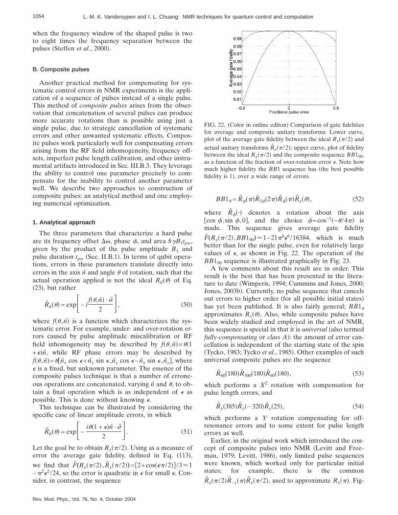
when the frequency window of the shaped pulse is twoto eight times the frequency separation between thepulses sSteffen et al., 2000d.

B. Composite pulses

Another practical method for compensating for sys-tematic control errors in NMR experiments is the appli-cation of a sequence of pulses instead of a single pulse.This method of composite pulses arises from the obser-vation that concatenation of several pulses can producemore accurate rotations than is possible using just asingle pulse, due to strategic cancellation of systematicerrors and other unwanted systematic effects. Compos-ite pulses work particularly well for compensating errorsarising from the RF field inhomogeneity, frequency off-sets, imperfect pulse length calibration, and other instru-mental artifacts introduced in Sec. III.B.3. They leveragethe ability to control one parameter precisely to com-pensate for the inability to control another parameterwell. We describe two approaches to construction ofcomposite pulses: an analytical method and one employ-ing numerical optimization.

1. Analytical approach

The three parameters that characterize a hard pulseare its frequency offset Dv, phase f, and area "gB1tpw,given by the product of the pulse amplitude B1 andpulse duration tpw sSec. II.B.1d. In terms of qubit opera-tions, errors in these parameters translate directly intoerrors in the axis n and angle u of rotation, such that theactual operation applied is not the ideal Rnsud of Eq.s23d, but rather

Rnsud = expF− ifsu,nd · sW

2G , s50d

where fsu , nd is a function which characterizes the sys-tematic error. For example, under- and over-rotation er-rors caused by pulse amplitude miscalibration or RFfield inhomogeneity may be described by fsu , nd=us1+edn, while RF phase errors may be described byfsu , nd=ufnx cos e+ ny sin e , ny cos e− nx sin e , nzg, wheree is a fixed, but unknown parameter. The essence of thecomposite pulses technique is that a number of errone-ous operations are concatenated, varying n and u, to ob-tain a final operation which is as independent of e aspossible. This is done without knowing e.

This technique can be illustrated by considering thespecific case of linear amplitude errors, in which

Rnsud = expF−ius1 + edn · sW

2G . s51d

Let the goal be to obtain Rxsp /2d. Using as a measure oferror the average gate fidelity, defined in Eq. s113d,we find that F„Rxsp /2d , Rxsp /2d…= f2+cossep /2dg /3<1−p2e2 /24, so the error is quadratic in e for small e. Con-sider, in contrast, the sequence

BB1u = RfspdR3fs2pdRfspdRxsud , s52d

where Rfs·d denotes a rotation about the axisfcos f , sin f ,0g, and the choice f=cos−1s−u /4pd ismade. This sequence gives average gate fidelity

F„Rxsp /2d ,BB190…<1–21p6e6 /16384, which is muchbetter than for the single pulse, even for relatively largevalues of e, as shown in Fig. 22. The operation of theBB190 sequence is illustrated graphically in Fig. 23.

A few comments about this result are in order. Thisresult is the best that has been presented in the litera-ture to date sWimperis, 1994; Cummins and Jones, 2000;Jones, 2003bd. Currently, no pulse sequence that cancelsout errors to higher order sfor all possible initial statesdhas yet been published. It is also fairly general; BB1u

approximates Rxsud. Also, while composite pulses havebeen widely studied and employed in the art of NMR,this sequence is special in that it is universal salso termedfully-compensating or class Ad: the amount of error can-cellation is independent of the starting state of the spinsTycko, 1983; Tycko et al., 1985d. Other examples of suchuniversal composite pulses are the sequence

R60s180dR300s180dR60s180d , s53d

which performs a X2 rotation with compensation forpulse length errors, and

Rys385dRys− 320dRys25d , s54d

which performs a Y rotation compensating for off-resonance errors and to some extent for pulse lengtherrors as well.

Earlier, in the original work which introduced the con-cept of composite pulses into NMR sLevitt and Free-man, 1979; Levitt, 1986d, only limited pulse sequenceswere known, which worked only for particular initialstates; for example, there is the common

Rxsp /2dR−yspdRxsp /2d, used to approximate Rxspd. Fig-

FIG. 22. sColor in online editond Comparison of gate fidelitiesfor average and composite unitary transforms: Lower curve,plot of the average gate fidelity between the ideal Rxsp /2d andactual unitary transforms Rxsp /2d; upper curve, plot of fidelitybetween the ideal Rxsp /2d and the composite sequence BB190,as a function of the fraction of over-rotation error e. Note howmuch higher fidelity the BB1 sequence has sthe best possiblefidelity is 1d, over a wide range of errors.



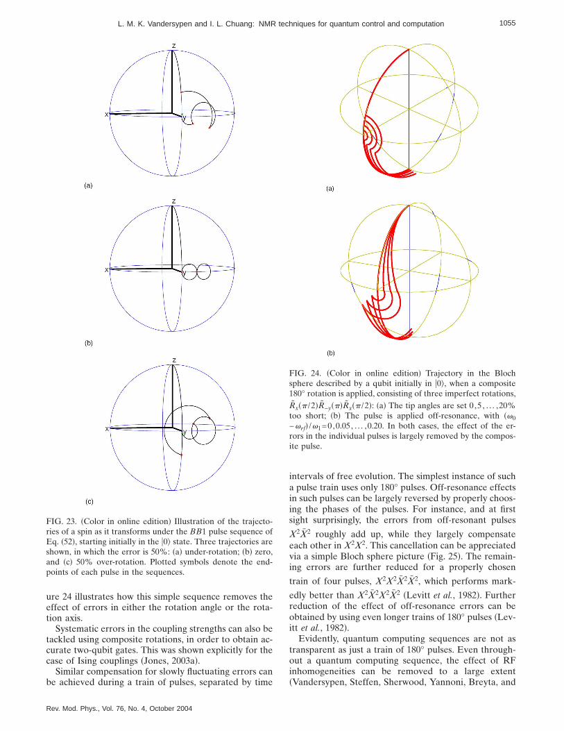
ure 24 illustrates how this simple sequence removes theeffect of errors in either the rotation angle or the rota-tion axis.

Systematic errors in the coupling strengths can also betackled using composite rotations, in order to obtain ac-curate two-qubit gates. This was shown explicitly for thecase of Ising couplings sJones, 2003ad.

Similar compensation for slowly fluctuating errors canbe achieved during a train of pulses, separated by time

intervals of free evolution. The simplest instance of sucha pulse train uses only 180° pulses. Off-resonance effectsin such pulses can be largely reversed by properly choos-ing the phases of the pulses. For instance, and at firstsight surprisingly, the errors from off-resonant pulses

X2X2 roughly add up, while they largely compensateeach other in X2X2. This cancellation can be appreciatedvia a simple Bloch sphere picture sFig. 25d. The remain-ing errors are further reduced for a properly chosen

train of four pulses, X2X2X2X2, which performs mark-

edly better than X2X2X2X2 sLevitt et al., 1982d. Furtherreduction of the effect of off-resonance errors can beobtained by using even longer trains of 180° pulses sLev-itt et al., 1982d.

Evidently, quantum computing sequences are not astransparent as just a train of 180° pulses. Even through-out a quantum computing sequence, the effect of RFinhomogeneities can be removed to a large extentsVandersypen, Steffen, Sherwood, Yannoni, Breyta, and

FIG. 23. sColor in online editiond Illustration of the trajecto-ries of a spin as it transforms under the BB1 pulse sequence ofEq. s52d, starting initially in the u0l state. Three trajectories areshown, in which the error is 50%: sad under-rotation; sbd zero,and scd 50% over-rotation. Plotted symbols denote the end-points of each pulse in the sequences.

FIG. 24. sColor in online editiond Trajectory in the Blochsphere described by a qubit initially in u0l, when a composite180° rotation is applied, consisting of three imperfect rotations,Rxsp /2dR−yspdRxsp /2d: sad The tip angles are set 0 ,5 , . . . ,20%too short; sbd The pulse is applied off-resonance, with sv0−vrfd /v1=0,0.05, . . . ,0.20. In both cases, the effect of the er-rors in the individual pulses is largely removed by the compos-ite pulse.



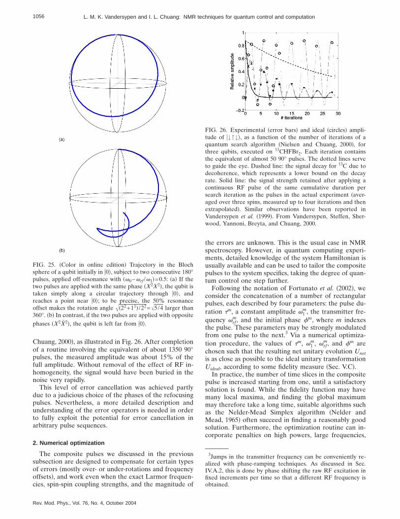
Chuang, 2000d, as illustrated in Fig. 26. After completionof a routine involving the equivalent of about 1350 90°pulses, the measured amplitude was about 15% of thefull amplitude. Without removal of the effect of RF in-homogeneity, the signal would have been buried in thenoise very rapidly.

This level of error cancellation was achieved partlydue to a judicious choice of the phases of the refocusingpulses. Nevertheless, a more detailed description andunderstanding of the error operators is needed in orderto fully exploit the potential for error cancellation inarbitrary pulse sequences.

2. Numerical optimization

The composite pulses we discussed in the previoussubsection are designed to compensate for certain typesof errors smostly over- or under-rotations and frequencyoffsetsd, and work even when the exact Larmor frequen-cies, spin-spin coupling strengths, and the magnitude of

the errors are unknown. This is the usual case in NMRspectroscopy. However, in quantum computing experi-ments, detailed knowledge of the system Hamiltonian isusually available and can be used to tailor the compositepulses to the system specifics, taking the degree of quan-tum control one step further.

Following the notation of Fortunato et al. s2002d, weconsider the concatenation of a number of rectangularpulses, each described by four parameters: the pulse du-ration tm, a constant amplitude v1

m, the transmitter fre-quency vrf

m, and the initial phase fm, where m indexesthe pulse. These parameters may be strongly modulatedfrom one pulse to the next.3 Via a numerical optimiza-tion procedure, the values of tm, v1

m, vrfm, and fm are

chosen such that the resulting net unitary evolution Unetis as close as possible to the ideal unitary transformationUideal, according to some fidelity measure sSec. V.Cd.

In practice, the number of time slices in the compositepulse is increased starting from one, until a satisfactorysolution is found. While the fidelity function may havemany local maxima, and finding the global maximummay therefore take a long time, suitable algorithms suchas the Nelder-Mead Simplex algorithm sNelder andMead, 1965d often succeed in finding a reasonably goodsolution. Furthermore, the optimization routine can in-corporate penalties on high powers, large frequencies,

3Jumps in the transmitter frequency can be conveniently re-alized with phase-ramping techniques. As discussed in Sec.IV.A.2, this is done by phase shifting the raw RF excitation infixed increments per time so that a different RF frequency isobtained.

FIG. 25. sColor in online editiond Trajectory in the Blochsphere of a qubit initially in u0l, subject to two consecutive 180°pulses, applied off-resonance with sv0−vrf /v1d=0.5: sad If thetwo pulses are applied with the same phase sX2X2d, the qubit istaken simply along a circular trajectory through u0l, andreaches a point near u0l; to be precise, the 50% resonanceoffset makes the rotation angle Îs22+11d /22=Î5/4 larger than360°. sbd In contrast, if the two pulses are applied with oppositephases sX2X2d, the qubit is left far from u0l.

FIG. 26. Experimental serror barsd and ideal scirclesd ampli-tude of u↓↑↓l, as a function of the number of iterations of aquantum search algorithm sNielsen and Chuang, 2000d, forthree qubits, executed on 13CHFBr2. Each iteration containsthe equivalent of almost 50 90° pulses. The dotted lines serveto guide the eye. Dashed line: the signal decay for 13C due todecoherence, which represents a lower bound on the decayrate. Solid line: the signal strength retained after applying acontinuous RF pulse of the same cumulative duration persearch iteration as the pulses in the actual experiment saver-aged over three spins, measured up to four iterations and thenextrapolatedd. Similar observations have been reported inVandersypen et al. s1999d. From Vandersypen, Steffen, Sher-wood, Yannoni, Breyta, and Chuang, 2000.



and negative or very long time periods, in order to pre-vent the algorithm from returning infeasible solutions.

Computation of Unet uses the fact that the Hamil-tonian during a fixed-amplitude RF pulse can be madetime independent by transforming into a referenceframe rotating at the transmitter frequency, as we haveseen in Sec. II.B.2. We shall call Hrot

m the effectiveHamiltonian in the frame rotating at vrf

m during segmentm. Given that vrf

m may be different for every segment ofthe pulse, it is most convenient to transform back to acommon reference frame at the end of every time slice.This can be the frame of the raw RF frequency, or thelaboratory frame of the n-spin system. In the lab frame,the time evolution during segment m is described by

Um = e−ivrfmok=1

n Izktm

e−iHrotm tm

. s55d

Since all Um are expressed in the same referenceframe, we can simply multiply them together to getUnet=pm Um and compare the result directly with Uideal,expressed in the laboratory frame as well.

Two representative examples of composite pulses de-signed for spin-selective rotations in homonuclear spinsystems are given in Fig. 27. The gate fidelity sSec. V.C.2dobtained with these two pulses is displayed in Fig. 28.Naturally, the fidelity is close to unity only near the reso-nance frequencies for which the gate was designed towork.

Composite pulses can thus effectively generate accu-rate single- and multiple-qubit Hamiltonians, using de-tailed knowledge of the system Hamiltonian and onlylimited knowledge about the errors. Often, however, fullknowledge of the system parameters is not available,and thus methods beyond composite pulses must be em-ployed.

C. Average-Hamiltonian theory

The average-Hamiltonian formalism offers a versatileframework for understanding how to effectively createor remove arbitrary terms in the Hamiltonian by peri-odic perturbations, without requiring full knowledge ofthe system dynamics. The refocusing sequences pre-sented in Sec. III.A.4 and more general multiple-pulsesequences designed to neutralize the effect of dipole-dipole couplings can be explained within this frame-work. Reduction of full dipole-dipole coupling given byEq. s5d to the simplified forms of Eqs. s6d and s7d canalso be understood with average-Hamiltonian theory.

Following Ernst et al. s1987d, we first introduce theMagnus expansion and then see how we can modify atime-independent Hamiltonian via a time-dependentperturbation. We use two concrete examples to illustratethe concepts.

1. The Magnus expansion

The essence of average-Hamiltonian techniques isthat the evolution Ustd under a time-dependent Hamil-tonian Hstd can be described by an effective evolution

under a time-independent average Hamiltonian H, un-der two conditions sHaeberlen and Waugh, 1968; Ernstet al., 1987d: sid Hstd is periodic and siid the observation isstroboscopic and synchronized with the period tc of Hstd.

We can then calculate H exactly from

Ustcd = exps− iHtcd , s56d

by diagonalizing Ustcd and taking the logarithm of theresulting eigenvalues sNielsen and Chuang, 2000d.

In practice, it is often more convenient to compute Happroximately. Let us assume that Hstd is piecewise con-stant fthe analysis can be easily generalized to the caseof continuously changing Hamiltonians sErnst et al.,1987dg: Hstd=Hk for o0

k−1ti, t,o0kti, and tc=o0

ntk, so

FIG. 27. The ideal RF waveform for two examples of stronglymodulated pulses: solid lines, amplitude of the waveform;dashed lines, phase. Details of the pulse parameters, as in Eq.s55d are listed below each wave form. The 6-ms time intervalwith zero RF power before and after the composite pulses isneeded due to experimental implementation issues. The com-posite pulse in sad performs a 90° rotation on one of the 13Cnuclei of 13C-labeled Alanine and the pulse in sbd performs asimultaneous 180° rotation on two 13C nuclei of 13C-labeledCrotonic acid. Courtesy of D. G. Cory. Reproduced from For-tunato et al., 2002.



Ustcd = exps− iHntnd ¯ exps− iH0t0d . s57d

Repeated application of the Baker-Campbell-Hausdorffrelation,

eBeA = expHA + B +12

fB,Ag+112

s†B,fB,Ag‡

+ †fB,Ag,A‡d + ¯J s58d

gives

H = Hs0d + Hs1d + Hs2d + ¯ , s59d

where

Hs0d =1

tchH0t0 + ¯ + Hntnj , s60d

Hs1d =− i

2tchfH1t1,H0t0g + fH2t2,H0t0g + fH2t2,H1t1g

+ ¯j , s61d

and so forth. This expansion, called the Magnus expan-sion sMagnus, 1954d, forms the basis of average-Hamiltonian theory.

2. Multiple-pulse decoupling

Let us consider a pulse sequence of n infinitesimallyshort pulses Uk separated by time intervals tk of freeevolution under the system Hamiltonian H0, and suchthat Un¯U2U1=I sfor pulses of finite length, the dura-tion of the pulses must also be included in the averaged.The pulses correspond to basis transformations, and we

can thus describe the system evolution via a sequence oftime intervals tk of free evolution under the Hamil-

tonian H0skd, with

H0s0d = H0, s62d

H0s1d = U1−1H0U1, s63d

H0s2d = U1−1U2

−1H0U2U1, s64d

and so forth. Note that the order in which the Uk areapplied to H0 is reversed and that the Uk themselves arereversed as well. If we let tc=o0

ntk, then the overalltransformation Ustcd is given by

Ustcd = exps− iH0sndtnd ¯ exps− iH0s0dt0d . s65d

We can now use the Magnus expansion of Eq. s59d and

Eqs. s60d and s61d, where we replace Hk by H0skd, to

obtain the average Hamiltonian H0 which describes thenet time evolution during tc. The zeroth-order averageHamiltonian is given by

Hs0d0 =

1

tcok=0

n

tkU1−1¯ Uk

−1H0Uk ¯ U1. s66d

The crux of average-Hamiltonian theory is that, by

properly choosing the pulse Uk, we can ensure that H0s0d

contains only the desired terms.Sophisticated pulse sequences sMehring, 1983d can

also remove undesired contributions from the higher-order terms in the expansion, although this is generally

harder since H0s1d ,H0

s2d, , . . . contain cross-terms between

the various H0skd. The commutators involved in thehigher-order terms do become smaller for shorter cycletimes, though, so fast cycles result in better averaging.

We also point out that pulse sequences which satisfy

H0skd = H0sn−kd s67d

or equivalently

Uk+1 = Un−k† s68d

contain no contributions of odd orders to H0,

Hskd0 = 0 for k = 1,3,5, . . . , s69d

and thus perform significantly better than other se-quences.

Let us now illustrate the operation of multiple-pulsedecoupling via two examples. First, the originalmultiple-pulse sequence for removal of dipole-dipole in-teractions is the WAHUHA-4 sequence sWaugh et al.,1968d,

tXtY2tYtXt , s70d

where the pulses are applied to all qubits involved, tstands for free evolution under the system Hamiltonianfor a duration t, and the unitaries are ordered from right

FIG. 28. sColor in online editiond Gate fidelity of the two ex-ample pulses of Fig. 27 as the resonance frequency of a testspin is varied. The solid sdashedd line is calculated with identitysdesired transformationd as the intended transformation. Thevertical dotted lines denote the actual chemical shifts for eachspin. Courtesy of D. G. Cory. Reproduced from Fortunato etal., 2002.



to left, as usual. The pulses rotate the Zeeman terms inthe Hamiltonian from −z to −y, −x, −y, and back to −zfsee Eqs. s62d–s64dg for a duration t, t, 2t, t, and t, re-spectively. The zeroth-order average Zeeman term isthus oriented along −sx+ y+ zd, with strength scaleddown by a factor 1/Î3. The dipolar Hamiltonian of Eq.s6d goes through the forms f3Iz

i Izj −Ii ·Ijg, f3Iy

i Iyj −Ii ·Ijg,

and f3Ixi Ix

j −Ii ·Ijg for equal durations, and is thus zero onaverage.

By selectively not pulsing specific qubits, it is also pos-sible to reintroduce some of the couplings as desired. InFig. 12, we already saw explicitly how to do this for Iz

i Izj

couplings.A second example is an extension of the conventional

spin-echo sequence sSec. V.A.4d to three-componentspin echoes sAugustine and Hahn, 1997d. In conven-tional echo sequences, 180° pulses about x or y removethe effect of a Hamiltonian of the form czsz. Now weask ourselves what sequence of pulses would freeze theevolution under a Hamiltonian of the form

H = cxsx + cysy + czsz, s71d

where cx ,cy ,cz are arbitrary coefficients. We can use Eq.s66d to verify that the sequence

X2tX2Y2tY2Z2tZ2t , s72d

or equivalently, after simplification,

X2tZ2tX2tZ2t , s73d

gives a zeroth-order average Hamiltonian Hs0d=0, andthus in effect corresponds to a three-component echosequence. Another way to show this is to note that

X2HX2 = + cxsx − cysy − czsz, s74d

Y2HY2 = − cxsx + cysy − czsz, s75d

Z2HZ2 = − cxsx − cysy + czsz. s76d

Clearly, H+X2HX2+Y2HY2+Z2HZ2=0, and so the se-quence of Eq. s72d gives, to zeroth order, no net evolu-tion. Again, if t is sufficiently short, the higher-ordercontributions will be negligible.

3. Reversing errors due to decoherence

Can we apply multiple-pulse sequences to reverse theeffect of interactions of a qubit with degrees of freedomin the environment? It is not clear a priori that this ispossible: standard average-Hamiltonian theory assumesthat we can manipulate both interacting particles in-volved, for instance, via RF pulses. However, we haveno control of degrees of freedom in the environment.

Remarkably, it is actually possible to remove the ef-fect of unwanted interactions with degrees of freedom inthe environment, even when applying operations to thesystem only sViola and Lloyd, 1998; Viola et al., 1998;Duan and Guo, 1999; Vitali and Tombesi, 1999d, pro-

vided the control operations are applied faster than thefluctuations. Knowledge about the nature of the interac-tions can be applied to simplify the sequence of decou-pling operations, and such knowledge can even be ex-perimentally extracted sByrd and Lidar, 2003d, in partusing a procedure known as process tomography, de-scribed in Sec. V.B.2.

If the fluctuations are faster than the accessible con-trol operations, errors can be corrected using quantumerror correction sShor, 1995; Steane, 1996; Nielsen andChuang, 2000d, or they can be prevented by encodingthe qubits in a subspace that is not affected by decoher-ence sZanardi and Rasetti, 1997; Lidar et al., 1998d. Thisis discussed further in Sec. V.D.

V. EVALUATION OF QUANTUM CONTROL

The pulse control methods presented in the last twosections can have impressive performance, but this isvery much contingent on having an accurate model ofthe system under control. A variety of techniques havebeen used in NMR to characterize the system dynamicsand to evaluate the performance of control sequences.In this section, we review some of these techniques, be-ginning with a set of standard experiments to determinehow quantum a qubit system is, then proceeding to to-mographic methods for fully characterizing system dy-namics, and concluding with fidelity metrics for controland their implications for scalability to large systems.

A. Standard experiments

In NMR spectroscopy as in atomic physics, a numberof standard experiments serve to test the quantum-mechanical behavior of a given system and to determinethe extent of its isolation from the environment ssee Sec.II.Cd, in terms of its phase coherence time T2 and itsenergy relaxation time T1, as well as the decay time inthe rotating frame T1r.

1. Coherent oscillations driven by a resonant field

The dynamics of a single spin, driven resonantly by acoherent field, were presented in Secs. II.B.1 and II.B.2.From Eq. s27d, we have that in the ideal case the RFfield induces transitions from u0l to u1l, where a qubitinitially in u0l will be found in u1l after an RF pulse ofduration tpw with probability

Prfu1lg = sin2sgB1tpw/2d = sin2sv1tpw/2d . s77d

The probability initially increases over time, until itreaches a maximum Prfu1lg=1 and then decreases again,by stimulated emission, a cycle which keeps repeatingitself.

Such oscillations of a two-level quantum systemdriven by a resonant field are known as Rabi oscillationssRabi, 1937d, and the Rabi frequency v1 /2p is propor-tional to the amplitude of the control field. Observationof Rabi oscillations is usually accepted as a signature ofquantum coherent behavior.



In reality, the envelope of the Rabi oscillation signal isalways damped, due to decoherence as well as instru-mental imperfections; measurement of this decay time isuseful, and known as a nutation experiment. In NMR,the Rabi decay time is often much shorter than the in-trinsic phase randomization time constant T2, due to theinhomogeneity across the macroscopic sample of the RFfield driving the Rabi oscillation. In other systems, theRabi decay time may be longer than T2, because sid along pulse can be seen as a concatenation of many 180°pulses, which can have a refocusing effect ssee Sec.III.A.4d, and siid the qubit is near ±z, where phase ran-domization has no effect, for roughly half the time dur-ing Rabi oscillations.

Coherent oscillations driven by a resonant field havebeen observed in NMR and in many atomic systems fora long time. Recently, however, observations of such co-herent dynamics have been made in other qubit systems,including systems made from Josephson junctions sNa-kamura et al., 1999d, molecular vibrational states sTeschand de Vivie-Riedle, 2002; Vala et al., 2002d, and exci-tons in semiconductor quantum dots sStievater et al.,2001d.

2. Coherent oscillations initiated by a kick

A quantum system starting off in a state that is not aneigenstate of the sstaticd system Hamiltonian will precessabout the quantization axis of the system Hamiltonian, amotion known as Larmor precession ssee Sec. II.A.1d.Such a situation could be realized by abruptly changingthe system Hamiltonian, e.g., by suddingly applying astrong static field along x instead of along z. Alterna-tively, and more realistically in NMR, Larmor precessioncan be initiated by suddenly kicking the qubit out of theHamiltonian eigenbasis. For a nuclear spin with Hamil-tonian −"v0Iz, as in Eq. s1d, this is done by applying a90° RF pulse, causing a transition for instance from u0lto su0l+ u1ld /Î2, which initiates the time evolution

ucstdl =eiv0t/2u0l + e−iv0t/2u1l

Î2, s78d

as illustrated in Fig. 2. Like Rabi oscillations, the obser-vation of Larmor precession is also a signature of quan-tum coherent behavior.

The Larmor precession is also damped, but in contrastto the Rabi decay time, the Larmor decay time, termedT2

*, is never longer than T2. Usually, T2*,T2; in particu-

lar, for NMR,

1

T2* =

1

T2+

1

T28, s79d

where T28 is the dephasing time constant due to staticmagnetic-field inhomogeneities or other instrumentalimperfections.

Larmor oscillations initiated by a kick have been ob-served recently in a variety of systems, including thosedriven resonantly mentioned earlier, and in addition asystem of charges in coupled quantum dots sHayashi et

al., 2003d. The oscillations can be observed directly if themeasurement basis lies in the x-y plane, as is the case inNMR. If the measurement takes place along ±z, wemust first change the basis via a second 90° pulse.

3. Ramsey interferometry

The double-pulse experiment

X t X , s80d

where time goes from right to left sas always, for unitarytransformations given in this articled and t denotes a freeevolution period, under the evolution operation e−iHsyst/"

is known as a Ramsey interference experiment sRamsey,1950d. Originally, this “method of separated oscillatoryfields” was applied to electronic states of molecularbeams traversing through two microwave excitationzones. In NMR, two pulses are involved, separated by adelay time t. Ramsey interference is most naturally de-scribed in the rotating frame of the RF field driving thetransition. If the qubit starts off along z, the first X pulserotates it to −y. Then the qubit precesses about z for atime t. Finally the second X pulse rotates the ±y com-ponent of the qubit state to 7z. Components along ±x atthe end of the interval t remain along ±x after the sec-ond X pulse.

If only a single qubit is considered and the RF field isexactly on-resonance with the qubit precession, the qu-bit stays in place in the rotating frame during the timeinterval in between the two pulses, and the final statedoes not vary with t. However, if the RF and the qubitare detuned in frequency by Dv, both the x and the zcomponents of the final state display a beating pattern asa function of Dvt, the so-called Ramsey fringes. Thedecay time of the envelope of the Ramsey fringes is T2

*,the same as that for Larmor precession.

For coupled qubits, the beating pattern contains infor-mation on the coupling strengths. This fact forms thebasis for two-dimensional correlation spectroscopysJeener, 1971; Ernst et al., 1987d, a widely used range oftwo-pulse techniques for molecular structure determina-tion.

4. Measurement of T2

The intrinsic T2 time can be extracted in an experi-ment that is based on Larmor or Ramsey experiments.Certain imperfections which cause the Ramsey or Lar-mor decay time T2

* to be smaller than T2 can be removedby applying refocusing sequences.

The simplest instance of such a refocusing sequenceconsists of a single 180° pulse applied halfway throughthe time interval of free evolution initiated by a 90°pulse. The entire sequence is thus

t

2X2 t

2X . s81d

A second X pulse should be added at the end if themeasurement takes place in the ±z basis. In multispin



systems, the pulses must be applied selectively to onespin, in order to measure the T2 of that spin.

The X2 refocusing pulse not only removes simple sca-lar spin-spin couplings, as described in Sec. III.A.4, butalso undoes the effect of spatial variations of the staticmagnetic field along z. Such field inhomogeneities causespins in different regions of the sample to become pro-gressively out of phase with each other during the firsttime interval t /2. As a result, their magnetic momentscancel each other out and the NMR signal vanishes. Pro-vided the magnetic-field variations are constant through-out the experiment, all the spins come back into phaseagain snow along +yd by the end of the second timeinterval t /2, because of the 180° refocusing pulse. As aresult, the signal recovers, producing the well-knownspin-echo. A generalization of this technique known asthree-component refocusing sSec. IV.C.2d undoes effectsfrom any static spin Hamiltonian terms.

The echo signal decays as a function of t, and thedecay time constant is a measure of T2. However, termsin the Hamiltonian fluctuating on a time scale shorterthan t are not removed by a single refocusing pulse.Their effect can still be removed if the fluctuations areslow compared to t /n and a train of n refocusing pulsesis applied, each preceded and followed by a time inter-val t /2n of free evolution. This so-called Carr-Purcellsequence sCarr and Purcell, 1954d,

t

2nX2 t

n¯ X2 t

nX2 t

2nX , s82d

produces a first echo along +y after t /n, a second echoalong −y after 2t /n, a third along +y after 3t /n, and soforth. The magnitude of the echo signal decays exponen-tially throughout this sequence, and the echo signal leftat the end of this sequence decreases exponentially as afunction of the total time t. To the extent that slow fluc-tuations in the Hamiltonian have been refocused, thedecay time constant is the intrinsic T2.

As we have seen in Sec. III of this review, small butfixed errors in the pulse amplitude or duration may ac-cumulate throughout a multiple-pulse sequence such asthe Carr-Purcell sequence. However, if the phase of therefocusing pulses is shifted by 90° with respect to theinitial 90° pulse, pulse length errors are compensated oneven-numbered echoes and are thus not cumulative. Inthis sequence,

t

2nY2 t

n¯ Y2 t

nY2 t

2nX , s83d

known as the Carr-Purcell-Meiboom-Gill or CPMG se-quence sMeiboom and Gill, 1958d, the echoes appear allalong −y. Again, the decay time constant of the echosignal gives T2.

Since T2 indicates how long a qubit can remain phasecoherent, it is usually called the coherence time, al-though the terms phase randomization time, dephasingtime, and transverse relaxation time are also used. InNMR, T2 is also known as the spin-spin relaxation time.

In any case, T2 is an important number for evaluatingthe potential of quantum computers, as the ratio of T2over the typical duration of a quantum logic gate ex-presses the number of operations that can be completedcoherently.

5. Measurement of T1

Energy exchange with the environment makes a qubitthat is out of equilibrium gradually return to thermalequilibrium. In thermal equilibrium, the qubit is in astatistical mixture of u0l and u1l, with probabilities set bythe temperature and the energy difference between u0land u1l. The time constant of this equilibration process,T1, is often called the energy relaxation time, the longi-tudinal relaxation time, or simply the relaxation time. InNMR, T1 is often termed the spin-lattice relaxation time.

Two standard experiments for measuring T1 are inver-sion recovery and saturation recovery. The sequence forthe inversion recovery experiment is

XtX2. s84d

The 180° pulse inverts the u0l and u1l probabilities, thenduring time t, relaxation takes place, and finally a 90°read-out pulse is applied if necessary si.e., when themeasurement basis is in the x-y planed. In saturation re-covery, a strong RF field is applied for a long enoughtime that it saturates the qubit transition and equalizesthe u0l and u1l probabilities. As in inversion recovery, theoriginal u0l and u1l populations are altered, and we canmonitor the populations’ return to their equilibriumvalue as a function of t. The time constant of this equili-bration process is T1.

Note that both the inversion recovery and saturationrecovery experiments bring the qubit out of equilibrium,but to a state that has no coherence. As a result, phaserandomization does not affect the equilibrationprocess—we measure purely the effect of energy ex-change with the bath. In contrast, Ramsey and spin-echoexperiments for measuring T2

* and T2 pick up contribu-tions from phase randomization both without and withenergy exchange with the bath. If energy exchangedominates phase randomization, the measured T2 is 2T1.

The relevance of T1 is twofold. First, it sets an upperbound for T2 and second, it tell us how much time wehave to perform a measurement in the hu0l , u1lj basis.Phase randomization does not change the u0l and u1lprobabilities, so T2 is irrelevant during such a measure-ment. In many cases, T1@T2, in which case we havemore time to measure than to perform coherent opera-tions.

6. Measurement of T1r

A third decay time useful to characterize the degreeof isolation between a qubit and the environment is T1r.This time constant can be measured via a techniquecalled spin locking, in which the spin is first rotated intothe x-y plane, say, by a Y pulse, and next continuousirradiation is applied, phase shifted by 90° with respect



to the pulse, so it is aligned with the spin state salong thex axisd:

RxscontinuousdY . s85d

The continuous irradiation along x locks the spin to thex axis, in the following sense. Whenever the spin startsto diverge from the x axis due to interactions with theenvironment, the RF field rotates it to the opposite sideof the x axis within a time p /v1. Provided that the spin isstill moving in the same direction after this time, it willthus return to the x axis snote that spin locking thus alsoinhibits evolution due to J couplings and moderate fre-quency offsetsd. Only if the spin moves in the oppositedirection after p /v1 will it continue to depart from the xaxis due to the rotation by the RF field. So the ampli-tude along x decays, and the decay time constant istermed T1r, known in NMR as the spin-lattice relaxationtime in the rotating frame.

We see thus that, whereas T2 is governed by low-frequency fluctuations in the environment and T1 de-pends on fluctuations at the Larmor frequency, the de-cay during spin locking arises from fluctuations at theRabi frequency used during spin locking. The spin-locking experiment thus gives additional information onthe spectral density of the interactions with the environ-ment.

B. Measurement of quantum states and gates

The standard experiments presented in the previoussection give only partial information on the system dy-namics. Here we show that in fact the full relaxationsuperoperator can be determined systematically by aprocedure known as process tomography, which buildsupon state tomography, as described below.

1. Quantum state tomography

The density matrix r completely describes our knowl-edge of the state of a system. Measurement of the den-sity matrix is therefore extremely helpful when testingor claiming the preparation of specific quantum states.

One-time measurement of each of n qubits, in a givenbasis of 2n states uml, gives very little information on r.All that can be inferred from a measurement outcome mis that PrfumlgÞ0.

Repeated measurements of n qubits, each time pre-pared in the same state and measured in the same basis,reveals the probability distribution for the measurementbasis states,

Prfumlg = kmuruml = Trsrumlkmud = TrsrMd , s86d

where M is an observable or measurement operator. Ifwe repeatedly measure each qubit in the hu0l , u1lj basis,we thus obtain all the diagonal entries of r, rii.

Quantum state tomography sChuang, Vandersypen, etal., 1998; Chuang et al., 1998a, 1998bd is a method thatallows all the elements of the density matrix r to bedetermined. This method consists of repeating the mea-

surement of the same state in various measurementbases, until all the elements of r can be determined, bysolving a set of linear equations. In practice, it is oftenmore convenient to first rotate the qubits via a unitarytransformation and then perform the measurement in afixed basis. This is equivalent to measuring in differentbases, since

TrfrsUMU†dg = TrfsU†rUdMg . s87d

Specifically, we can expand the density matrix of asingle qubit r as

Fr00 r01

r10 r11G = r00u0lk0u + r01u0lk1u + r10u1lk0u + r11u1lk1u .

s88d

Measurements of a single qubit in the hu0l , u1lj basis giveus r00 and r11=1−r00. However, after changing basis viaa 90° rotation about x, transforming r to XrX†, we ob-tain access to Imsr10d=−Imsr01d. Similarly, measurementafter transformation by Y reveals Resr10d=Resr01d.Thus, by measuring the qubit state first directly, thenmeasuring the same state again after an X read-outpulse, and then again after a Y read-out pulse, we canreconstruct r completely.

Similarly, for n qubits, we can expand r as

r = oi=0

2n−1

oj=0

2n−1

rijuilkju s89d

and choose a set of basis changes that gives access to all4n−1 degrees of freedom in r.

However, it is much easier to find a suitable set ofbasis changes if we use the Pauli expansion of r insteadof Eq. s89d. The Pauli expansion for a single-qubit stateis

r = c0s0 + c1s1 + c2s2 + c3s3, s90d

where c0=1 for normalization, and we use s0=I /2, s1=sx /2, s2=sy /2, s3=sz /2. Measurement in the compu-tational basis, described by the observables s0±s3, givesus Prsu0ld= sc0+c3d /2, and Prsu1ld= sc0−c3d /2 so we canextract c3. Since

XrX† = c0s0 + c1s1 − c3s2 + c2s3, s91d

YrY† = c0s0 + c3s1 + c2s2 − c1s3, s92d

we indeed obtain sc0±c2d /2 after applying X andsc07c1d /2 after using Y.

For n qubits, Eq. s90d generalizes to

r = oi=0

3

oj=0

3

¯ ok=0

3

cij¯k si ^ sj ^ ¯ ^ sk, s93d

where c00¯0=1. Measurement in the computational basisis described by observables of the form

ss0 ± s3d ^ ss0 ± s3d ^ ¯ ^ ss0 ± s3d s94d

and returns the probabilities



oi,j,. . .,kPh0,3j

±cij¯k

2n . s95d

For example, for two qubits, these are

Prsu00ld = sc00 + c03 + c30 + c33d/4, s96d

Prsu01ld = sc00 − c03 + c30 − c33d/4, s97d

Prsu10ld = sc00 + c03 − c30 − c33d/4, s98d

Prsu11ld = sc00 − c03 − c30 + c33d/4. s99d

After measurement of the four Prfumlg, we can solve forc03,c30,c33 from this overdetermined set of linear equa-tions. Again, we can determine the other cij¯k by trans-formation of the corresponding sij¯k to an observable,for instance,

X1Y2ss0 + s2d ^ ss0 + s1dX1†Y2

†

= ss0 + s3d ^ ss0 − s3d . s100d

We end this discussion of state tomography with threeadditional comments:

First, in order to obtain all the basis-state probabilitiesas in Eqs. s96d–s99d, we must each time read out all thequbits. If it is only possible to read out any one singlequbit in each experiment, we obtain n bit-wise probabili-ties instead of 2n basis-state probabilities, giving spin-spin correlations. The measurement operators are thenof the form

2n−1fs0 ^ s0 ^ ss0 ± s3d ^ ¯ ^ s0g s101d

and we measure probabilities

12

sc0¯000¯0 ± c0¯030¯0d . s102d

It is now no longer possible to rotate arbitrary compo-nents of r into observable positions using just single-qubit rotations. Two-qubit gates are necessary to obtainall cij¯k.

Second, the measurement basis obviously need not bethe computational basis. In NMR experiments, for in-stance, the single-qubit measurement operator can bewritten as −is1−s2. For two coupled spins, the measure-ment operators are

2s− is1 − s2d ^ ss0 ± s3d , s103d

ss0 ± s3d ^ 2s− is1 − s2d , s104d

and so forth. Since NMR experiments are normally per-formed on a large ensemble of molecules, the expecta-tion value of the observables can be read out by acquir-ing a single spectrum. The four operators in Eq. s104dcorrespond to the four lines in the spectrum of a two-spin system stwo doubletsd. Phase-sensitive detectionpermits us to separately record the real and imaginarycomponent of each spectral line and distinguish s1 ands2 contributions.

Third, errors in the gates used for changing basis dur-ing state tomography lead to a measured density matrixwhich differs from the actual state of the system. If theerrors are known and can be modeled accurately, theycan be incorporated in the state tomography procedureand the actual state can nevertheless be determined ac-curately.

Quantum state tomography has been experimentallyimplemented in many atomic systems, notably the earlywork mapping out photon states sSmithey et al., 1993dand vibrational cat states of trapped atoms sMeekhof etal., 1996d. Recently, it has become a common tool usedto evaluate NMR states sChuang, Vandersypen, et al.,1998; Chuang et al., 1998bd, states of optical photon qu-bits sThew et al., 2002d, and even vibrational states ofmolecules sSkovsen et al., 2003d.

2. Quantum process tomography

Now that we know how to determine experimentallythe state of a quantum system, it is only a short step tothe characterization of a quantum process, such as aquantum logic gate, communication channel, storage de-vice, and so forth. In general, let us consider a quantum-mechanical black box whose input may be an arbitraryquantum state, and whose output is the result of theinternal dynamics of the black box, as well as interac-tions with the outside world. Then can we ascertain thetransfer function of this black box?

The answer is yes sChuang and Nielsen, 1997; Poyatoset al., 1997; D’Ariano and Lo Presti, 2001; Boulant et al.,2003d. The outline of the procedure is to first determinethe output state of the black box for a set of input stateswhich form a basis for the system Hilbert space, andthen to use the fact that quantum mechanics is linear tocompute the entire transfer function from this finite setof input-output pairs.

An arbitrary quantum state transformation is a linearmap E,

r °Esrd

TrfEsrdg, s105d

where we can express Esrd in the operator-sum represen-tation or Kraus representation sKraus, 1983; Nielsen andChuang, 2000d

Esrd = ok

AkrAk† . s106d

This is an alternative to the superoperator formalismwidely used in NMR sErnst et al., 1987d. The Ak areoperators acting on the system alone, yet E completelydescribes the possible state changes of the system, in-cluding unitary operations, generalized measurements,and decoherence sfor trace-preserving processes,oi Ak

†Ak=1d. The expansion of Eq. s106d is in generalnot unique. In fact, we can always describe E using a

fixed set of operators Ak which form a basis for the setof operators on the state space, so that sChuang andNielsen, 1997d



Esrd = op,q

xpqAprAq† , s107d

where xpq is a positive Hermitian matrix. Since the Akare fixed, E is completely described by x. In general, xwill contain 16n−4n independent real parameters, wheren is the number of qubits.

In order to determine x experimentally, we choose abasis of 4n linearly independent density matrices rjwhich span the system Hilbert space, and determineEsrjd for each j. We can then write down a set of linearequations of the form of Eq. s107d, where we plug in themeasurement outcomes Esrjd and solve for the xmn.

The most convenient choice for the rj depends on theimplementation of the qubits and on the observables, aswas the case for state tomography. Clearly, the effortneeded to perform quantum process tomography in-creases even more rapidly with the number of qubitsthan quantum state tomography. This procedure hasbeen used experimentally only for one- and two-qubitNMR sChilds et al., 2001; Boulant et al., 2003d andoptical-photon systems sAltepeter et al., 2003; Mitchellet al., 2003d.

The operation elements Ak in the operator sum rep-resentation of Eq. s106d can describe arbitrary quantumoperations, but among these a select subset are useful toidentify. For example, when Ak is a unitary matrix, thiscorresponds to perfect, closed-system Hamiltonian evo-lution. Phase damping sT2d is described by

A0 = F1 0

0 ÎgG, A1 = F0 0

0 Î1 − gG , s108d

and amplitude damping sT1d by

A0 = F1 0

0 ÎgG, A1 = F0 Î1 − g

0 0G , s109d

where g,e−t/t parametrizes the strength of the damping,for time t, in terms of a time constant t. These and otherrelaxation parameters sNielsen and Chuang, 2000d canbe obtained by process tomography.

Such results can, in turn, be useful for approximatenumerical simulation of relaxation and decoherenceprocesses in spin systems. Phase damping and energyrelaxation can be simulated in alternation with unitaryevolution under the system and control Hamiltonian,taking sufficiently short time slices to obtain a good ap-proximation of the true dynamics. This permits an n-spinsystem to be simulated using n4n steps, compared to 16n

for fully general quantum operations. Experimental re-sults have shown this method to be predictive of thesystem dynamics throughout sequences containing hun-dreds of RF pulses sVandersypen, 2001; Vandersypen etal., 2001d.

C. Fidelity of quantum states and gates

The methods of the previous section give us fullknowledge of the system state and dynamics, but some-

times a more succinct measure for comparing theoreticalexpectations with experimental measurements is useful.This can be provided by quantum state fidelity and gatefidelity.

1. Quantum state fidelity

One elementary goal of quantum control is to createsome pure state ucl. However, suppose the final output isinstead the pure state ufl. Does ufl represent ucl withhigh fidelity?

Classically, the fidelity of two probability distributionshpxj and hqxj is given by Fspx ,qxd=ox

Îpxqx; when theyare equal, the fidelity is one. The analogous quantummeasure of fidelity for two pure states ucl and ufl is

Fsucl, ufld = ukfuclu , s110d

which is simply the absolute value of the overlap be-tween the two states.

More generally, the output state of a control sequenceis often described by a density matrix r; this is usefulbecause density matrices can describe classical statisticalmixtures of quantum states, arising from decoherenceprocesses, for example. The fidelity between a pure stateucl and a mixed state r is

Fsucl,rd = Îkcurucl , s111d

which reduces to Eq. s110d when r= uflkfu.The most general case is the fidelity between two den-

sity matrices, r and s, which is defined as sNielsen andChuang, 2000d

Fss,rd ; TrÎÎsrÎs . s112d

Despite the apparent asymmetry in this expression, it isactually symmetric in r and s and, furthermore, reducesproperly to Eq. s111d when one density matrix is pure.

Note that in the literature, sometimes the square ofEq. s110d is defined as the fidelity sBowdrey et al., 2002d;this departs from the usual classical definition for fidel-ity, but is convenient because Fsucl , ufld2 can be inter-preted as the probability that a system in the state ufl isfound to be in the state ucl when measured in thehucl , uc'lj basis. Such probabilities are meaningful in theaccuracy thresholds discussed in Sec. V.D.

Other metrics for comparing two states have beenused to quantify the relative error between theoreticaland experimental states, such as the simple two-normsVandersypen et al., 2000d and other expressions sFortu-nato et al., 2002d. These were used because the diagonalelements of the density matrix were suppressed; suchmetrics are inferior to the fidelity measure, which shouldbe used when possible, due to its direct connection toquantum information measures and fault-tolerancetheorems.

It is worthwhile to consider a specific example relatingcontrol precision to state fidelity. Suppose we desireucl= u1l, but obtain ufl=Rysp+edu0l=−sin e /2u0l+cos e /2u1l<−e /2u0l+ s1−e2 /8du1l. The resulting error



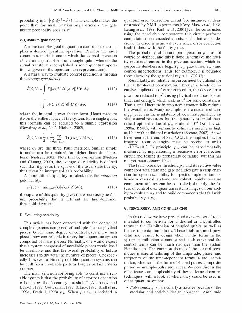
probability is 1− ukf uclu2=e2 /4. This example makes thepoint that, for small rotation angle errors e, the gatefailure probability goes as e2.

2. Quantum gate fidelity

A more complex goal of quantum control is to accom-plish a desired quantum operation. Perhaps the mostcommon scenario is one in which the desired operationU is a unitary transform on a single qubit, whereas theactual transform accomplished is some quantum opera-tion E sgiven in the operator sum representationd.

A natural way to evaluate control precision is throughthe average gate fidelity

FsE,Ud =E F„ucl,U†EsuclkcudU…

2 dc s113d

=E kcuU†EsuclkcudUucl dc , s114d

where the integral is over the uniform sHaard measuredc on the Hilbert space of the system. For a single qubit,this formula can be reduced to a simple expressionsBowdrey et al., 2002; Nielsen, 2002d,

FsE,Ud =12

+112 o

k=h1,2,3jTrfUskU†Esskdg , s115d

where sk are the three Pauli matrices. Similar simpleformulas can be obtained for higher-dimensional sys-tems sNielsen, 2002d. Note that by convention sNielsenand Chuang, 2000d, the average gate fidelity is definedsuch that it goes as the square of the usual state fidelity;thus it can be interpreted as a probability.

A more difficult quantity to calculate is the minimumgate fidelity,

FsE,Ud = minuclF„Uucl,Esuclkcud…; s116d

the square of this quantity gives the worst-case gate fail-ure probability that is relevant for fault-tolerancethreshold theorems.

D. Evaluating scalability

This article has been concerned with the control ofcomplex systems composed of multiple distinct physicalpieces. Given some degree of control over a few suchpieces, how controllable is a very large quantum systemcomposed of many pieces? Normally, one would expectthat a system composed of unreliable pieces would itselfbe unreliable, and that the overall probability of failureincreases rapidly with the number of pieces. Unexpect-edly, however, arbitrarily reliable quantum systems canbe built from unreliable parts as long as certain criteriaare met.

The main criterion for being able to construct a reli-able system is that the probability of error per operationp be below the “accuracy threshold” sAharonov andBen-Or, 1997; Gottesman, 1997; Kitaev, 1997; Knill et al.,1998a; Preskill, 1998d pth. When p,pth is satisfied, a

quantum error correction circuit ffor instance, as dem-onstrated by NMR experiments sCory, Mass, et al., 1998;Leung et al., 1999; Knill et al., 2001dg can be constructedusing the unreliable components; this circuit performscomputations on encoded qubits, such that a net de-crease in error is achieved even when error correctionitself is done with the faulty gates.

The probability of failure per operation p must ofcourse be defined, and this is done in terms of the fidel-ity metrics discussed in the previous section, which in-corporate decoherence se.g., T1, T2, gate times, etc.d andcontrol imperfections. Thus, for example, p is boundedfrom above by the gate fidelity pø1−FsE ,Ud2.

Remarkably, no reliable resources need be utilized forthe fault-tolerant construction. Through k levels of re-cursive application of error correction, the device errorp can be reduced to p2k

, using physical resources sspace,time, and energyd, which scale as dk for some constant d.Thus a small increase in resources exponentially reducesthe overall error. Many assumptions are made in obtain-ing pth, such as the availability of local, fast, parallel clas-sical control resources, but the generally accepted theo-retical optimal value of pth is about 10−4 sKnill et al.,1998a, 1998bd, with optimistic estimates ranging as highas 10−3 with additional restrictions sSteane, 2002d. As wehave seen at the end of Sec. V.C.1, this implies that, forinstance, rotation angles must be precise to order,Î10−4=10−2. In principle, pth can be experimentallymeasured by implementing a recursive error correctioncircuit and testing its probability of failure, but this hasnot yet been accomplished.

The fault-tolerance threshold pth and its relative valuecompared with state and gate fidelities give a crisp crite-rion for system scalability for specific implementations.Modern classical systems are robust mainly becausecomponent failures can be controlled; similarly, the fu-ture of control over quantum systems hinges on our abil-ity to evaluate pth and to build components that fail withprobability p,pth.

VI. DISCUSSION AND CONCLUSIONS

In this review, we have presented a diverse set of toolsintended to compensate for undesired or uncontrolledterms in the Hamiltonian of coupled qubits, as well asfor instrumental limitations. These tools are most pow-erful and easiest to design when all the terms in thesystem Hamiltonian commute with each other and thecontrol terms can be much stronger than the systemHamiltonian. The common theme of the control tech-niques is careful tailoring of the amplitude, phase, andfrequency of the time-dependent terms in the Hamil-tonian, whether in the form of shaped pulses, compositepulses, or multiple-pulse sequences. We now discuss theeffectiveness and applicability of these advanced controltechniques, with a look at where they could be used inother quantum systems.

• Pulse shaping is particularly attractive because of themodular and scalable design approach. Amplitude



profiles are selected from a library of standard orspecially designed shapes in order to minimize cross-talk sfrequency-selective pulsesd and coupling effectssself-refocusing pulsesd. Robustness to experimentalimperfections can also be considered in the choice ofpulse shape. Once suitable amplitude profiles havebeen chosen, the pulse lengths are set as short aspossible while maintaining qubit selectivity. Thesame amplitude profiles and pulse lengths are thenused throughout the pulse sequence.Remaining cross-talk effects can be further reducedat a small cost squadratic in the number of qubitsd.From the amplitude profiles and pulse lengths, unin-tended phase shifts produced by single RF pulses aswell as off-resonance effects during simultaneouspulses can be precomputed, once for every pair ofqubits.The main disadvantage of the standard pulse-shapingtechniques is that often the coupled evolution duringthe pulses sin particular 90° pulses or simultaneouspulsesd cannot be completely frozen. The remainingcoupled evolution can be unwound to a large extentduring the time intervals before and after the pulse,but such reversal is never perfect because the RFterms in the Hamiltonian, Ix

i and Iyi , do not commute

with the coupling terms, Izi Iz

j . Furthermore, shapedpulses must often be quite long in order to remainspin-selective, which means that decoherence hasmore effect. This problem clearly gets worse as theLarmor frequencies of the spins approach each other.Nevertheless, the combination of pulse-shaping andphase-ramping techniques has been very successfulin practice. It has enabled the implementation of themost complex sequences of operations realized todate, acting on up to seven nuclear spins.

• Composite pulses have proven to be a versatile toolin NMR spectroscopy, mostly for compensating sys-tematic errors such as RF field strength variationsand frequency offsets. Another useful application ofcomposite pulses is the effective creation of unitaryoperators which are otherwise not accessible or noteasily accessible. A good example is the composite zrotation, created from a sequence of x and y rota-tions.Even so, the use of shardd composite pulses in NMRquantum computing experiments has been limited sofar. Their main drawback is that in multispin homo-nuclear molecules, single-frequency but high-powerand rectangular pulses will rotate spins in a large fre-quency window, about an axis and over angles whichdepend on RF field strength and the respective reso-nance offsets. This severely limits straightforward ap-plication of hard composite pulses in homonuclearspin systems.Nevertheless, it is in principle possible to take advan-tage of the differences in resonance offsets in orderto rotate one spin while the other spins undergo nonet rotation. Such effective frequency selectivity de-spite the use of hard pulses was demonstrated in a

quantum computation on a homonuclear two-spinsystem, first using single hard pulses sJones andMosca, 1999d and later using composite hard pulsessCummins and Jones, 2000d.The same idea underlies the operation of compositepulses tailored to achieve any rotation of one ormore spins about an independent axis, using detailedknowledge of the system Hamiltonian. Furthermore,short, high-power pulses can be used, so the effect ofdecoherence is reduced compared to the case of thelong, low-power shaped pulses. Even more attractivehere is the fact that all the coupling terms can beeffectively frozen and that other types of cross-talk,such as Bloch-Siegert effects, are automatically takencare of, unlike the case of shaped pulses.The main disadvantage of such strongly modulatedcomposite pulses is that the time needed to find near-optimal pulse parameters increases exponentiallywith the number of qubits n, as it involves computingunitary matrices of size 2n by 2n. Nevertheless, forsmall numbers of qubits, this technique can be veryuseful.

• Average-Hamiltonian techniques underlie the opera-tion of widely used multiple-pulse refocusing se-quences. In the context of liquid NMR quantumcomputing, couplings are of the form Iz

i Izj and refo-

cusing sequences consist simply of a train of 180°pulses. Such refocusing sequences are an essential in-gredient of all NMR quantum computing experi-ments involving more than two spins.More complex decoupling sequences exist to removethe effect of coupling Hamiltonians of a differentform, as is the case of solid-state NMR and manyother qubit implementations. Even errors arisingfrom interactions with the environment, i.e., deco-herence, can be removed using multiple-pulse se-quences.In all cases, the refocusing operations se.g., the 180°pulsesd must be fast compared to the fluctuationsthey are intended to cancel, and they must also berepeated at a rate faster than the fluctuations.

• Perspective. In early NMR quantum computing ex-periments on heteronuclear spin systems, whereshort, high-power RF pulses were used, errors in thetime evolution were usually dominated by variousinstrumental limitations. Most experiments onhomonuclear systems, in contrast, made use of long,low-power pulses, and were limited by cross-talk andcoupling effects. As the pulse techniques for copingwith limitations of the Hamiltonian and instrumenta-tion became more advanced, the field reached thepoint where errors due to imperfect quantum controlwere smaller than errors caused by decoherence.Reaching this point in many-qubit systems must be aprime objective for any implementation of quantumcomputers, along with reduction of decoherence it-self. Quantum information and computation theoryoffers a common language which can facilitate trans-fer and translation of the techniques for coherent



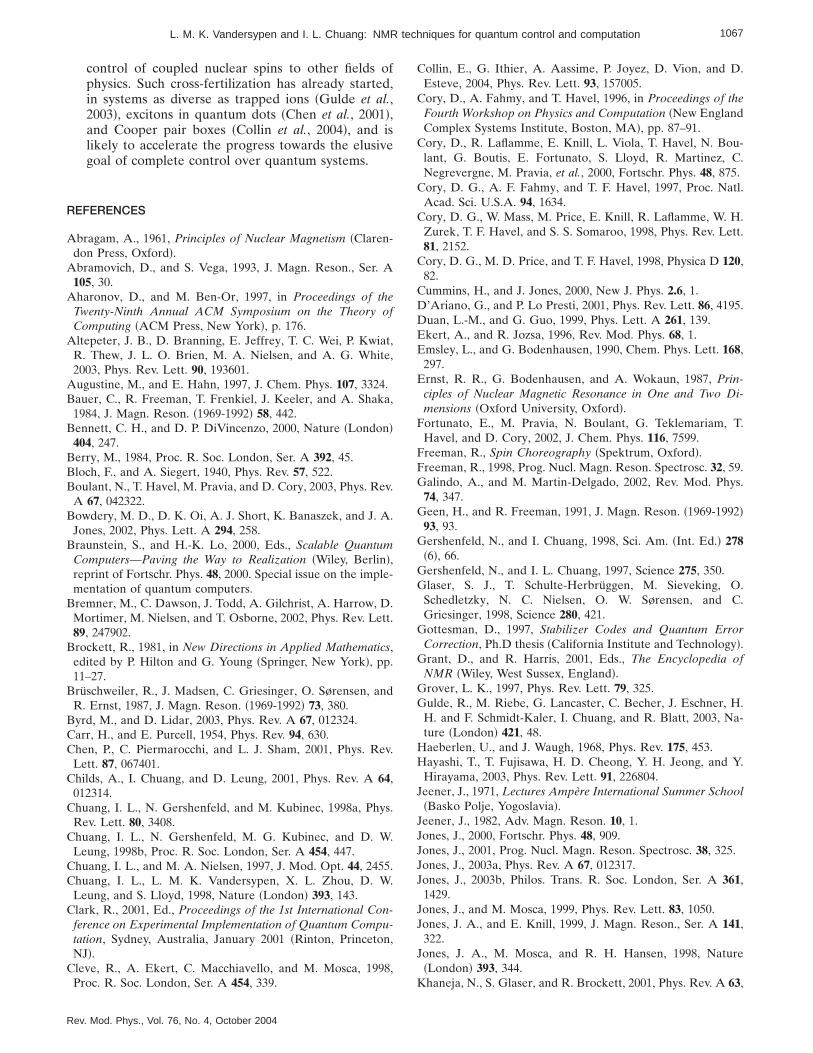
control of coupled nuclear spins to other fields ofphysics. Such cross-fertilization has already started,in systems as diverse as trapped ions sGulde et al.,2003d, excitons in quantum dots sChen et al., 2001d,and Cooper pair boxes sCollin et al., 2004d, and islikely to accelerate the progress towards the elusivegoal of complete control over quantum systems.

REFERENCES

Abragam, A., 1961, Principles of Nuclear Magnetism sClaren-don Press, Oxfordd.

Abramovich, D., and S. Vega, 1993, J. Magn. Reson., Ser. A105, 30.

Aharonov, D., and M. Ben-Or, 1997, in Proceedings of theTwenty-Ninth Annual ACM Symposium on the Theory ofComputing sACM Press, New Yorkd, p. 176.

Altepeter, J. B., D. Branning, E. Jeffrey, T. C. Wei, P. Kwiat,R. Thew, J. L. O. Brien, M. A. Nielsen, and A. G. White,2003, Phys. Rev. Lett. 90, 193601.

Augustine, M., and E. Hahn, 1997, J. Chem. Phys. 107, 3324.Bauer, C., R. Freeman, T. Frenkiel, J. Keeler, and A. Shaka,

1984, J. Magn. Reson. s1969-1992d 58, 442.Bennett, C. H., and D. P. DiVincenzo, 2000, Nature sLondond

404, 247.Berry, M., 1984, Proc. R. Soc. London, Ser. A 392, 45.Bloch, F., and A. Siegert, 1940, Phys. Rev. 57, 522.Boulant, N., T. Havel, M. Pravia, and D. Cory, 2003, Phys. Rev.

A 67, 042322.Bowdery, M. D., D. K. Oi, A. J. Short, K. Banaszek, and J. A.

Jones, 2002, Phys. Lett. A 294, 258.Braunstein, S., and H.-K. Lo, 2000, Eds., Scalable Quantum

Computers—Paving the Way to Realization sWiley, Berlind,reprint of Fortschr. Phys. 48, 2000. Special issue on the imple-mentation of quantum computers.

Bremner, M., C. Dawson, J. Todd, A. Gilchrist, A. Harrow, D.Mortimer, M. Nielsen, and T. Osborne, 2002, Phys. Rev. Lett.89, 247902.

Brockett, R., 1981, in New Directions in Applied Mathematics,edited by P. Hilton and G. Young sSpringer, New Yorkd, pp.11–27.

Brüschweiler, R., J. Madsen, C. Griesinger, O. Sørensen, andR. Ernst, 1987, J. Magn. Reson. s1969-1992d 73, 380.

Byrd, M., and D. Lidar, 2003, Phys. Rev. A 67, 012324.Carr, H., and E. Purcell, 1954, Phys. Rev. 94, 630.Chen, P., C. Piermarocchi, and L. J. Sham, 2001, Phys. Rev.

Lett. 87, 067401.Childs, A., I. Chuang, and D. Leung, 2001, Phys. Rev. A 64,

012314.Chuang, I. L., N. Gershenfeld, and M. Kubinec, 1998a, Phys.

Rev. Lett. 80, 3408.Chuang, I. L., N. Gershenfeld, M. G. Kubinec, and D. W.

Leung, 1998b, Proc. R. Soc. London, Ser. A 454, 447.Chuang, I. L., and M. A. Nielsen, 1997, J. Mod. Opt. 44, 2455.Chuang, I. L., L. M. K. Vandersypen, X. L. Zhou, D. W.

Leung, and S. Lloyd, 1998, Nature sLondond 393, 143.Clark, R., 2001, Ed., Proceedings of the 1st International Con-

ference on Experimental Implementation of Quantum Compu-tation, Sydney, Australia, January 2001 sRinton, Princeton,NJd.

Cleve, R., A. Ekert, C. Macchiavello, and M. Mosca, 1998,Proc. R. Soc. London, Ser. A 454, 339.

Collin, E., G. Ithier, A. Aassime, P. Joyez, D. Vion, and D.Esteve, 2004, Phys. Rev. Lett. 93, 157005.

Cory, D., A. Fahmy, and T. Havel, 1996, in Proceedings of theFourth Workshop on Physics and Computation sNew EnglandComplex Systems Institute, Boston, MAd, pp. 87–91.

Cory, D., R. Laflamme, E. Knill, L. Viola, T. Havel, N. Bou-lant, G. Boutis, E. Fortunato, S. Lloyd, R. Martinez, C.Negrevergne, M. Pravia, et al., 2000, Fortschr. Phys. 48, 875.

Cory, D. G., A. F. Fahmy, and T. F. Havel, 1997, Proc. Natl.Acad. Sci. U.S.A. 94, 1634.

Cory, D. G., W. Mass, M. Price, E. Knill, R. Laflamme, W. H.Zurek, T. F. Havel, and S. S. Somaroo, 1998, Phys. Rev. Lett.81, 2152.

Cory, D. G., M. D. Price, and T. F. Havel, 1998, Physica D 120,82.

Cummins, H., and J. Jones, 2000, New J. Phys. 2.6, 1.D’Ariano, G., and P. Lo Presti, 2001, Phys. Rev. Lett. 86, 4195.Duan, L.-M., and G. Guo, 1999, Phys. Lett. A 261, 139.Ekert, A., and R. Jozsa, 1996, Rev. Mod. Phys. 68, 1.Emsley, L., and G. Bodenhausen, 1990, Chem. Phys. Lett. 168,

297.Ernst, R. R., G. Bodenhausen, and A. Wokaun, 1987, Prin-

ciples of Nuclear Magnetic Resonance in One and Two Di-mensions sOxford University, Oxfordd.

Fortunato, E., M. Pravia, N. Boulant, G. Teklemariam, T.Havel, and D. Cory, 2002, J. Chem. Phys. 116, 7599.

Freeman, R., Spin Choreography sSpektrum, Oxfordd.Freeman, R., 1998, Prog. Nucl. Magn. Reson. Spectrosc. 32, 59.Galindo, A., and M. Martin-Delgado, 2002, Rev. Mod. Phys.

74, 347.Geen, H., and R. Freeman, 1991, J. Magn. Reson. s1969-1992d

93, 93.Gershenfeld, N., and I. Chuang, 1998, Sci. Am. sInt. Ed.d 278

s6d, 66.Gershenfeld, N., and I. L. Chuang, 1997, Science 275, 350.Glaser, S. J., T. Schulte-Herbrüggen, M. Sieveking, O.

Schedletzky, N. C. Nielsen, O. W. Sørensen, and C.Griesinger, 1998, Science 280, 421.

Gottesman, D., 1997, Stabilizer Codes and Quantum ErrorCorrection, Ph.D thesis sCalifornia Institute and Technologyd.

Grant, D., and R. Harris, 2001, Eds., The Encyclopedia ofNMR sWiley, West Sussex, Englandd.

Grover, L. K., 1997, Phys. Rev. Lett. 79, 325.Gulde, R., M. Riebe, G. Lancaster, C. Becher, J. Eschner, H.

H. and F. Schmidt-Kaler, I. Chuang, and R. Blatt, 2003, Na-ture sLondond 421, 48.

Haeberlen, U., and J. Waugh, 1968, Phys. Rev. 175, 453.Hayashi, T., T. Fujisawa, H. D. Cheong, Y. H. Jeong, and Y.

Hirayama, 2003, Phys. Rev. Lett. 91, 226804.Jeener, J., 1971, Lectures Ampère International Summer School

sBasko Polje, Yogoslaviad.Jeener, J., 1982, Adv. Magn. Reson. 10, 1.Jones, J., 2000, Fortschr. Phys. 48, 909.Jones, J., 2001, Prog. Nucl. Magn. Reson. Spectrosc. 38, 325.Jones, J., 2003a, Phys. Rev. A 67, 012317.Jones, J., 2003b, Philos. Trans. R. Soc. London, Ser. A 361,

1429.Jones, J., and M. Mosca, 1999, Phys. Rev. Lett. 83, 1050.Jones, J. A., and E. Knill, 1999, J. Magn. Reson., Ser. A 141,

322.Jones, J. A., M. Mosca, and R. H. Hansen, 1998, Nature

sLondond 393, 344.Khaneja, N., S. Glaser, and R. Brockett, 2001, Phys. Rev. A 63,



032308.Khaneja, N., S. Glaser, and R. Brockett, 2002, Phys. Rev. A 65,

032301.Khitrin, A., V. Ermakov, and B. Fung, 2002, Chem. Phys. Lett.

360, 161.Kitaev, A. Y., 1997, Russ. Math. Surveys 52, 1191.Knill, E., R. Laflamme, R. Martinez, and C. Negrevergne,

2001, Phys. Rev. Lett. 86, 5811.Knill, E., R. Laflamme, R. Martinez, and C.-H. Tseng, 2000,

Nature sLondond 404, 368.Knill, E., R. Laflamme, and W. H. Zurek, 1998a, Science 279,

342.Knill, E., R. Laflamme, and W. H. Zurek, 1998b, Proc. R. Soc.

London, Ser. A 454, 365.Kraus, K., 1983, States, Effects, and Operations: Fundamental

Notions of Quantum Theory, Lecture Notes in Physics, No.190 sSpringer, Berlind.

Kup~e, E., and R. Freeman, 1995, J. Magn. Reson., Ser. A 112,261.

Leibfried, D., R. Blatt, C. Monroe, and D. J. Wineland, 2003,Rev. Mod. Phys. 75, 281.

Leskowitz, G., N. Ghaderi, R. Olsen, and L. Mueller, 2003, J.Chem. Phys. 119, 1643.

Leung, D., L. Vandersypen, X. Zhou, M. Sherwood, C. Yan-noni, and I. Chuang, 1999, Phys. Rev. A 60, 1924.

Leung, D. W., I. L. Chuang, F. Yamaguchi, and Y. Yamamoto,2000, Phys. Rev. A 61, 042310.

Levitt, M., 1986, Prog. Nucl. Magn. Reson. Spectrosc. 18, 61.Levitt, M., 2001, Spin Dynamics sWiley, West Sussex, En-

glandd.Levitt, M., and R. Freeman, 1979, J. Magn. Reson. s1969-1992d

33, 473.Levitt, M., R. Freeman, and T. Frenkiel, 1982, J. Magn. Reson.

s1969-1992d 47, 328.Lidar, D. A., I. L. Chuang, and K. B. Whaley, 1998, Phys. Rev.

Lett. 81, 2594.Linden, N., H. Barjat, R. Carbajo, and R. Freeman, 1999,

Chem. Phys. Lett. 305, 28.Linden, N., E. Kup~e, and R. Freeman, 1999, Chem. Phys.

Lett. 311, 321.Lloyd, S., 1995, Sci. Am. sInt. Ed.d 273 s4d, 140.Magnus, W., 1954, Commun. Pure Appl. Math. 7, 649.Maklin, Y., G. Schön, and A. Schirman, 2001, Rev. Mod. Phys.

73, 357.Meekhof, D., C. Monroe, B. King, W. Itano, and D. Wineland,

1996, Phys. Rev. Lett. 76, 1796.Mehring, M., 1983, High Resolution NMR Spectroscopy in Sol-

ids sSpringer, Berlind.Meiboom, S., and D. Gill, 1958, Rev. Sci. Instrum. 29, 688.Mitchell, M., C. Ellenor, S. Schneider, and A. Steinberg, 2003,

Phys. Rev. Lett. 91, 120402.Nakamura, Y., Y. A. Pashkin, and J. S. Tsai, 1999, Nature

sLondond 398, 786.Nelder, J., and R. Mead, 1965, Comput. J. sUKd 7, 308.Nielsen, M. A., 2002, Phys. Lett. A 303, 249.Nielsen, M., and I. Chuang, 2000, Quantum Computation and

Quantum Information sCambridge University, Cambridge,Englandd.

Nielsen, M. A., E. Knill, and R. Laflamme, 1998, NaturesLondond 396, 52.

Osborne, I., and R. Coontz, 2002, Science 298, 1353.Patt, S., 1991, J. Magn. Reson. s1969-1992d 96, 94.Pauly, J., P. L. Roux, and D. Nishimura, 1991, IEEE Trans.

Med. Imaging 10 s1d, 53.Poyatos, J. F., J. I. Cirac, and P. Zoller, 1997, Phys. Rev. Lett.

78, 390.Preskill, J., 1998, Proc. R. Soc. London, Ser. A 454, 385.Rabi, I., 1937, Phys. Rev. 51, 652.Ramsey, N., 1950, Phys. Rev. 78, 695.Redfield, A., 1957, IBM J. Res. Dev. 1, 19.Shor, P. W., 1995, Phys. Rev. A 52, R2493.Skovsen, E., H. Stapelfeldt, S. Juhl, and K. Molmer, 2003,

Phys. Rev. Lett. 91, 090406.Slichter, C. P., 1996, Principles of Magnetic Resonance

sSpringer, Berlind.Smithey, D., M. Beck. M. Raymer, and A. Faridani, 1993,

Phys. Rev. Lett. 70, 1244.Somaroo, S., C. H. Tseng, T. F. Havel, R. Laflamme, and D. G.

Cory, 1999, Phys. Rev. Lett. 82, 5381.Sørenson, O., 1989, Prog. Nucl. Magn. Reson. Spectrosc. 21,

503.Steane, A., 1998, Rep. Prog. Phys. 61, 117.Steane, A., 2002, quant-ph/0207119.Steane, A. M., 1996, Phys. Rev. Lett. 77, 793.Steffen, M., 2003, A Prototype Quantum Computer Using

Nuclear Spins in Liquid Solution, Ph.D. thesis sStanford Uni-versityd.

Steffen, M., L. Vandersypen, and I. Chuang, 2000, J. Magn.Reson., Ser. A 146, 369.

Steffen, M., L. Vandersypen, and I. Chuang, 2001, IEEE Mi-cro. 21 s2d, 24.

Stievater, T., X. Li, D. Steel, D. Katzer, D. Park, C. Pierma-rocchi, and L. Sham, 2001, Phys. Rev. Lett. 87, 133603.

Tesch, C. M., and R. de Vivie-Riedle, 2002, Phys. Rev. Lett. 89,157901.

Thew, R., K. Nemoto, A. White, and W. Munro, 2002, Phys.Rev. A 66, 012303.

Tycko, R., 1983, Phys. Rev. Lett. 51, 775.Tycko, R., H. Cho, E. Schneider, and A. Pines, 1985, J. Magn.

Reson. s1969-1992d 61, 90.Vala, J., Z. Amitay, B. Zhang, S. R. Leone, and R. Kosloff,

2002, Phys. Rev. A 66, 062316.Vandersypen, L. M. K., 2001, Experimental Quantum Compu-

tation with Nuclear Spins in Liquid Solution, Ph.D. thesissStanford Universityd.

Vandersypen, L. M. K., M. Steffen, G. Breyta, C. S. Yannoni,R. Cleve, and I. L. Chuang, 2000, Phys. Rev. Lett. 85, 5452.

Vandersypen, L. M. K., M. Steffen, G. Breyta, C. S. Yannoni,M. H. Sherwood, and I. L. Chuang, 2001, Nature sLondond414, 883.

Vandersypen, L. M. K., M. Steffen, M. H. Sherwood, C. Yan-noni, G. Breyta, and I. L. Chuang, 2000, Appl. Phys. Lett. 76,646.

Vandersypen, L. M. K., C. Yannoni, and I. Chuang, 2002, inEncyclopedia of Nuclear Magnetic Resonance: SupplementaryVolume, edited by D. Grant and R. Harris sWiley, West Sus-sex, Englandd, p. 687.

Vandersypen, L. M. K., C. S. Yannoni, M. H. Sherwood, and I.L. Chuang, 1999, Phys. Rev. Lett. 83, 3085.

Viola, L., E. Knill, and S. Lloyd, 1998, Phys. Rev. Lett. 82,2417.

Viola, L., and S. Lloyd, 1998, Phys. Rev. A 58, 2733.Vitali, D., and P. Tombesi, 1999, Phys. Rev. A 59, 4178.Walmsley, I., and H. Rabitz, 2003, Phys. Today 56 s8d, 43.Warren, W., 1984, J. Chem. Phys. 81, 5437.Waugh, J., L. Huber, and U. Haeberlen, 1998, Phys. Rev. Lett.



20, 180.Wieman, C., D. Pritchard, and D. Wineland, 1999, Rev. Mod.

Phys. 71, S253.Wimperis, S., 1994, J. Magn. Reson., Ser. B 109, 221.Yannoni, C., M. Sherwood, L. Vandersypen, M. Kubinec, D.

Miller, and I. Chuang, 1999, Appl. Phys. Lett. 75, 3563.

Zanardi, P., and M. Rasetti, 1997, Phys. Rev. Lett. 79, 3306.Zeilinger, A., 1999, Rev. Mod. Phys. 71, S288.Zhang, W., and D. Cory, 1998, Phys. Rev. Lett. 80, 1324.Zutic, I., J. Fabian, and S. D. Sarma, 2004, Rev. Mod. Phys. 76,

323.



NMR techniques for quantum control and computation · 2009-10-19 · NMR techniques for quantum...

Documents

Transcript of NMR techniques for quantum control and computation · 2009-10-19 · NMR techniques for quantum...