Draft: 9/5/02

NMR Properties of Reservoir Fluids

George Hirasaki1, Matthias Appel2, Justin Freeman2 1 Rice University 2 Shell International E&P Co

NMR PROPERTIES OF RESERVOIR FLUIDS ..............................................1

RELAXATION.......................................................................................................................................2 MECHANISMS ..............................................................................................................2 INTRA-MOLECULAR DIPOLE-DIPOLE INTERACTIONS.....................................................4 INTER-MOLECULAR DIPOLE-DIPOLE INTERACTIONS .....................................................5 SPIN-ROTATION INTERACTIONS....................................................................................6 DEAD CRUDE OILS ......................................................................................................7 LIVE CRUDE OILS ........................................................................................................9 EFFECT OF DISSOLVED OXYGEN................................................................................11 BRINE AND WATER-BASED DRILLING FLUIDS...........................................................11 RESERVOIR GAS ........................................................................................................12

DIFFUSION..........................................................................................................................................14 CONTINUUM TRANSPORT: FICK'S LAWS OF DIFFUSION ............................................14 SELF-DIFFUSION........................................................................................................15 DIFFUSION EQUATION ...............................................................................................15 MEASUREMENT TECHNIQUES - DIFFUSION AND SELF-DIFFUSION .............................16 SELF-DIFFUSION MEASUREMENTS BY CPMG WITH CONSTANT MAGNETIC FIELD GRADIENTS................................................................................................................18 SELF DIFFUSION OF HYDROCARBON SYSTEMS ..........................................................19 CONSTITUENT VISCOSITY MODEL .............................................................................20

HYDROGEN INDEX...........................................................................................................................21 DEFINITION OF HYDROGEN INDEX.............................................................................21 HI OF BRINES ............................................................................................................22 HI OF GAS .................................................................................................................23 CORRELATIONS FOR HYDROGEN INDEX ....................................................................23 HI OF HEAVY OILS ....................................................................................................24 HI FOR HYDROCARBON MIXTURES AND LIVE OILS...................................................24

REFERENCES .....................................................................................................................................27

1

INTRODUCTION The response measured by NMR well logging tools is from the fluids in the pore space. The initial amplitude is a function of the total porosity, fluid saturation and the hydrogen index of the fluids. The relaxation of the response is a function of the surface relaxation, bulk relaxation, and diffusion in a field gradient. Surface relaxation is discussed elsewhere. Here we will discuss bulk fluid relaxation, self-diffusion of bulk fluids and hydrogen index (HI).

The estimation of porosity usually assumes that the initial response in a NMR well log is a measure of the total fluids in the pore space. However, if the wait time of the pulse sequence is not long enough compared to the longest T1 of the fluids, then the fluids will not be completely polarized and the initial amplitude will need to be corrected for the effect of partial polarization. Also, a heavy oil may have a portion of its relaxation time distribution shorter than the echo spacing and thus not be detected by the CPMG echo sequence. This will result in an apparent HI that is less than the actual HI. In such cases, the HI of the oil should be measured in the laboratory with the same echo spacing as used in the well log.

The estimation of the bulk volume irreducible (BVI) requires that the T2 distribution below the T2 cut-off be distinguished between that due to water and that due to fast relaxing components of the crude oil. Also, estimation of the oil and/or gas saturation and the oil viscosity require that the contributions of the different fluids to the T2 distribution be distinguished. Water, oil and gas generally have different diffusion coefficients and their contributions to the T2 distribution can be estimated by performing a sequence of measurements with different echo spacing.

Laboratory measurements of fluid properties are often made at ambient conditions. However, petroleum reservoirs are often at elevated temperatures and pressures. The effect of reservoir temperature and dissolved gas on viscosity is generally recognized. However, methane, even when dissolved in the oil, relaxes by a different mechanism than the dead oil and thus it is necessary to account for the gas/oil ratio in the estimation of the relaxation time. Also, dissolved gases can significantly lower the HI of live oils. RELAXATION

Mechanisms

NMR relaxation describes the return of the magnetization to equilibrium after the Boltzmann population of oriented magnetic moments has been disturbed. A short duration or "pulse" of electromagnetic radiation at the Larmor frequency usually accomplishes the perturbation from equilibrium.

NMR relaxation processes can be categorized into two main classes: (i) dispersion of irradiated energy (T1-relaxation), and (ii) the loss of phase coherence of spin groups caused by local variations of the Larmor frequency (T2-relaxation).

The spin-lattice or longitudinal relaxation process (T1) depends on the exchange of energy between the spin system and its surroundings to allow relaxation of the spin system towards its thermal equilibrium state (given by a certain temperature and magnetic field strength) after the population of the Zeeman energy levels have been disturbed by radio-frequency pulses. This energy exchange is

2

realized through dynamics of the molecular lattice such as molecular rotation, diffusion, or vibration.

In contrast to this, the spin-spin or transverse relaxation process (T2) does not require energy transitions but depends on local (on a molecular level) variations of the magnetic field strength which in turn lead to variations of the Larmor frequency of individual spins. The greater the dispersion of Larmor frequencies, the faster the phase coherence of precessing spins disappears.

All NMR relaxation processes require electromagnetic fields that fluctuate over molecular distances. For NMR relaxation, two types of fields are important: (i) a time varying magnetic field that interacts with the nuclear magnetic dipole moments and (ii) a gradient of the electric field that interacts with the electric quadrupole moment of the nucleus. In oil field applications, only the magnetic resonance effect of protons is currently exploited. Therefore, this discussion needs only to focus on the dipolar interaction caused by time varying magnetic fields, since protons do not possess any quadrupole moment.

There are several possible sources for time varying magnetic fields. The strongest magnetic fields (on a molecular level) are caused by unpaired electrons as found in paramagnetic materials such as dissolved molecular oxygen and paramagnetic ions such as iron and manganese. The latter are primarily responsible for surface relaxation on the pore walls of rocks.

The tumbling motion of molecules is an additional source of time varying magnetic fields. The superposition of the magnetic fields of individual spins leads to interactions between magnetic moments and creates a randomly varying field at the site of the nucleus.

For our discussion of the NMR response of reservoir fluids, two kinds of interactions between magnetic moments are important. In liquids, the molecular distances between spin groups are small enough such that short-range dipolar interactions contribute significantly to spin relaxation. This process is known as a dipole-dipole interaction. This includes both intramolecular and intermolecular interactions. Intermolecular dipole-dipole interactions are a very strong function of the intermolecular distances i.e., the density. When the density of magnetic moments is reduced, as in the case in gases, this interaction becomes less important.

For liquid systems, dipolar interactions between the spins are the main source of the local magnetic field modifications that govern the T2 relaxation process. Molecular rotation, diffusion, or vibrations of the lattice (that are the source for the T1 relaxation process) also contribute to T2 relaxation. For low viscosity liquids, the fast molecular tumbling averages out the dipolar fields from neighboring spins, the dipolar contribution to the T2 relaxation process is minimized and the T2 relaxation process will be as slow as the T1 relaxation, i.e., T1=T2. This process is often referred to as motional narrowing.

However, for asphaltenes, resins and other structures of higher molecular weight, the molecular motion might not be fast enough to average the dipolar field of neighboring spin systems. This leads to a spin-spin relaxation time, T2, which is shorter than the spin-lattice relaxation time, T1.

For gases where small spherical molecules are relatively free to rotate, spin rotation is another important interaction of the magnetic moments. This mechanism is

3

between the nuclear spin and the molecular magnetic moment that arises from variations of the angular momentum of a rotating molecule.

Since any one of the various mechanisms can accomplish the relaxation to equilibrium, the net relaxation rate can be expressed as the sum of the individual rates:

1,2 1,2 1,2 1,2

1 1 1

b d dr d dtT T T T− −

= + +1

sr

, (1)

where 1,2 denotes either T1 or T2, b denotes bulk fluid, d-dr denotes intra-molecular dipole-dipole rotation, d-dt denotes intermolecular dipole-dipole translation, and sr denotes spin-rotation.

Intra-molecular dipole-dipole interactions

Molecular collisions of a molecule with its neighbors result in a time dependent change of the orientation of a pair of neighboring protons. This random motion has a characteristic time, called the correlation time, cτ . This random change of orientation with time can also be described by a rotational diffusivity, . The rotational diffusivity is a function of the viscosity of the medium, temperature and molecular size. The relation between the relaxation times and the rotational correlation time for intra-molecular, dipole-dipole interactions is as follows (Cowan, 1997),

rD

( ) ( )

( ) ( )

2 2 21

2 2 22

2 2 4

2 6

1 2 / 3 8 / 31 1 2

1 5 / 3 2 / 311 1 2

9 , for a diatomic molecule20 4

co c o c

co c o c

o

MT

MT

Mr

τω τ ω τ

τω τ ω τ

µ γπ

= +

+ +

= + ++ +

=

(2)

where oω is the Larmor frequency, oµ is the magnetic permeability of free space, is Planck's constant divided by 2π , γ is the gyromagnetic ratio for the 1H proton, and r is the distance between the nearest protons in the molecule. Only the nearest neighbors are considered because the coefficient, M2, is a function of distance to the inverse sixth power.

Liquids with fast motions (e.g., low viscosity, high temperature, and small molecules) relative to the Larmor frequency have a relaxation rate that is proportional to the rotational correlation time. We can see this by taking the limit of short correlation time behaviour of the above equations:

2

1 2

1 1 10 ,3 c o cM

T Tτ ω τ= = 1. (3)

This limit where T1 =T2 is called the fast motion, adiabatic motional narrowing, or extreme narrowing approximation.

4

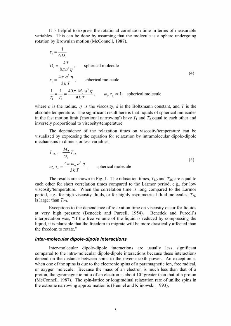
It is helpful to express the rotational correlation time in terms of measurable variables. This can be done by assuming that the molecule is a sphere undergoing rotation by Brownian motion (McConnell, 1987).

3

3

32

1 2

16

, spherical molecule84 , spherical molecule

31 1 40 , 1, spherical molecule

9

cr

r

c

o c

Dk TDaa

k TM a

T T k T

τ

π η

π ητ

π η ω τ

=

=

=

= =

(4)

where a is the radius, η is the viscosity, k is the Boltzmann constant, and T is the absolute temperature. The significant result here is that liquids of spherical molecules in the fast motion limit ('motional narrowing') have T1 and T2 equal to each other and inversely proportional to viscosity/temperature.

The dependence of the relaxation times on viscosity/temperature can be visualized by expressing the equation for relaxation by intramolecular dipole-dipole mechanisms in dimensionless variables.

21,2 1,2

34 , spherical molecule3

Do

oo c

MT T

ak T

ω

π ω ηω τ

=

= (5)

The results are shown in Fig. 1. The relaxation times, T1D and T2D are equal to each other for short correlation times compared to the Larmor period, e.g., for low viscosity/temperature. When the correlation time is long compared to the Larmor period, e.g., for high viscosity fluids, or for highly asymmetrical fluid molecules, T1D is larger than T2D.

Exceptions to the dependence of relaxation time on viscosity occur for liquids at very high pressure (Benedek and Purcell, 1954). Benedek and Purcell’s interpretation was, “If the free volume of the liquid is reduced by compressing the liquid, it is plausible that the freedom to migrate will be more drastically affected than the freedom to rotate.”

Inter-molecular dipole-dipole interactions

Inter-molecular dipole-dipole interactions are usually less significant compared to the intra-molecular dipole-dipole interactions because these interactions depend on the distance between spins to the inverse sixth power. An exception is when one of the spins is due to the electronic spins of a paramagnetic ion, free radical, or oxygen molecule. Because the mass of an electron is much less than that of a proton, the gyromagnetic ratio of an electron is about 103 greater than that of a proton (McConnell, 1987). The spin-lattice or longitudinal relaxation rate of unlike spins in the extreme narrowing approximation is (Hennel and Klinowski, 1993),

5

( 2

2 2 22

21,

2132

o

d dt

NT kT

µ γ η γ−

= ) (6)

where 2γ and are the gyromagnetic ratio and number concentration of the second species of molecule. Since the gyromagnetic ratio is raised to the second power, the contribution of a paramagnetic species may be significant even though its concentration is small.

2N

2N

Since dipolar interactions dominate the NMR relaxation for gas-free reservoir fluids, it is useful to combine the intra- and intermolecular contributions. For low viscosity fluids and temperatures above ambient, the motional narrowing condition is generally well fulfilled. Assuming further that intra- and intermolecular motions are uncorrelated, the dipolar relaxation rate can be expressed as

4 2 3 6

6 32 1

1 1 2 315

a N bT T k b a T

.π γ π = = +

η (7)

where a is the molecular radius and b is the distance between the nearest protons.

In reference to the first authors, the derivation of the above relation is often referred to as Bloembergen, Pound, Purcell (1948) ("BPP") theory.

Spin-rotation interactions

Spin-rotation interaction becomes a significant contribution to the relaxation of small molecules and/or gases where the motions are so fast that the dipole-dipole relaxation rate becomes small. The molecular collisions in dilute gases are assumed to be binary as the time between collisions becomes large compared to the time two molecules are interacting with each other. The relaxation times within the extreme narrowing approximation are as follows (Gordon, 1966):

1 2

1 1

N J

k TT T vρ σ

= ∝ (8)

where, Nρ is the number density of the gas, is the velocity of the gas, and v Jσ is the cross section for the transfer of angular momentum. The bracket represents the average of the product. Kinetic theory can be used to approximate the ensemble average molecular speed of a dilute gas.

8k Tvmπ

= (9)

where is the reduced mass of the collision pair. It is assumed that the average of the product of speed and cross-section is equal to the product of the respective average quantities. Thus the relaxation time can be expressed as a function of density and temperature.

m

6

( )( )

1 2

1 2

1 1

1N J

Jn

N N

k TT T T

TT TTT

ρ σ

σρ ρ

= ∝

= ∝ ∝

(10)

where n is an empirical exponent equal to about 1.5 for methane (Jameson et al., 1991).

An alternate derivation (Hubbard, 1963b) expresses the spin-rotation relaxation rate in terms of viscosity and temperature.

( ) ( )

( ) ( )

2 22

1 1 221 2

2

2

1 2

2 2 22

1 22 31 2

2 21 1 , ,3

2 , / 9

34

6

21 1 , ,12

o o

o o

o o

I k T C C

T T

aD

I Da k Tk TD

a

I C C k TT T a

τ τ τ ω τ

τ τ τ

τ

π η

τ τ ω τπ η

⊥

⊥

+= = <<

= =

=

=

+∴ = = <<

1

1

(11)

where theτ are the various correlation times, C C, ⊥ are the components of the spin-rotation coupling tensor, and I is the moment of inertia of the spherical molecule.

The significance of this expression is that the relaxation rate for the spin-rotation mechanism has a dependence on temperature, viscosity, and molecular size that is the inverse of the relationship for intra-molecular dipole-dipole interactions.

Dead Crude Oils

Dead crude oils relax primarily by intramolecular dipole-dipole interactions. Therefore, the direct correlation between NMR relaxation rates and fluid viscosity has often been exploited in formation evaluation. The original correlation for the relaxation time of dead crude oils and viscosity standards at ambient conditions was expressed only as a function of viscosity (Morriss et al., 1994). The correlation was modified to express it as a function of viscosity and temperature:

2,LM 0.9

1.2 , at ambient temperature. Morriss . (1997)T eη

= t al (12)

2, LM1.2 , Vinegar (1995)298

TTη

= (13)

0.9 0.9

2,LM 0.9

1.2 0.0071 , Zhang . (1998)(298)

T TT eη η

= =

t al (14)

7

In these equations, T2,LM is the log-mean value (in seconds) of the transverse relaxation time spectrum, η the viscosity in cp, and T the temperature in Kelvin.

Fig. 2 shows measured T1,LM and T2,LM relaxation times as a function of fluid viscosity over temperature for various alkanes, gas-free oils and viscosity standards. Lo et al. (1999) showed that the approximation developed by Morriss et al. underestimates the relaxation times of degassed normal alkanes. The NMR relaxation of such fluids might be enhanced because of the additional paramagnetic relaxation brought about by the dissolved oxygen. This effect is discussed in more detail below. Experimentally, Lo et al. quantified the impact of the dissolved oxygen on the relaxation behaviour of alkanes and derived the following correlation between the relaxation time and viscosity of oxygen-free alkanes:

1,LM 0.00956 .TTη

= (15)

This correlation was based on measured T1,LM relaxation times. However, no significant difference was found between T1,LM and T2,LM measurements for these alkanes (Zega et al., 1989; Lo, 1999). This correlation was compared with the base oil of an OBM as a function of temperature and pressure in Fig. 3. The experimental data for T2 as a function of pressure show that temperature and pressure variations affect the relaxation behaviour of the gas-free OBM in different ways. While the variation of relaxation time with temperature at a given pressure can be adequately described with the correlation for oxygen-free alkanes, pressure variation results in different trends than that expected from the correlation. The reduction in relaxation time is much reduced compared to the increase in viscosity. This experiment illustrates the decoupling between viscosity and relaxation. The effect is related to molecular free volume. As outlined in the section on intramolecular dipolar interactions, increases in pressure will first reduce the free volume of the system, and hence reduce the intermolecular motion, before it reduces the intramolecular motions, i.e., the freedom of a molecule to rotate. Since the intramolecular term generally contributes more to relaxation than the intermolecular one, and viscosity is governed by intermolecular actions, pressure increases reduce relaxation time less than it reduces viscosity. The above equations based on crude oils and on alkanes have been widely used in formation evaluation. However, it needs to be emphasized that these equations are only valid for gas-free liquids.

Differences between T1 and T2 measurements have been found for viscous crude oils. This difference is a function of the Larmor frequency, Fig. 2, and may be due to heavy components of the crude oil not being in the fast motion limit. Fig. 2 shows that T1/T2 is larger for larger viscosity (i.e., longer correlation time) and higher Larmor frequency. The dependence of the T1 on Larmor frequency can be correlated by normalizing the relaxation time and viscosity with the Larmor frequency in the manner suggested by the section on intramolecular dipole-dipole interactions.

1,2N 1,20

0

N

2(MHz)

2(MHz)

T T

T T

ωωη η

=

=

(16)

The normalized T1,LM relaxation time as a function of the normalized viscosity is shown in Fig. 4. This normalization to 2 MHz collapses all T1,LM data of crude oils to

8

a single curve. For low viscosities, the measured T1,LM data agree well with the correlation between viscosity and T2,LM derived for gas-free crude oils, and therefore illustrate the validity of the fast motion approximation for this viscosity range. At higher viscosities, the measured T1,LM values depart from the T2,LM correlation. Furthermore, the experimental T1,LM show a lower plateau value instead of the theoretically expected increase of T1. In Fig. 4, a dashed line shows the theoretical prediction for T1 of a system with a single molecular correlation time. Given that T1 will reach its minimum when the inverse of the Larmor frequency is equal to the molecular correlation time, the observed lower plateau of the T1 data illustrates that crude oils need to be characterized by a spectrum of molecular correlation times.

The relaxation time distribution of crude oils (Morriss et al., 1997) is typically significantly broader than that of a pure hydrocarbon as illustrated in Fig. 5. Here the T2 distribution of a 23 cp, 30° API gravity crude oil is compared with that of n-hexadecane. The shape of the distribution is important for fluid identification, e.g., for the distinction between crude oils and oil-based mud filtrates (Prammer et al., 2001).

Heavy oils may have fast relaxing components that relax significantly before the first echo occurs and thus are not fully detected. This will not only result in a misinterpretation of the relaxation time distribution but also result in an underestimation of the hydrogen index (LaTorraca et al., 1998 &1999; Mirotchnik et al., 1999). In Fig. 6, the relaxation time distributions of a 302 cp, 19° API gravity oil are shown that are measured at 30° C by inversion recovery and CPMG with echo spacing of 0.24 ms and 2 ms. The T2 distribution is truncated for short relaxation times at the longer echo spacing because of the loss of information. Also, the difference between T1 and T2 is apparent even at a Larmor frequency of 2 MHz for this viscous crude oil.

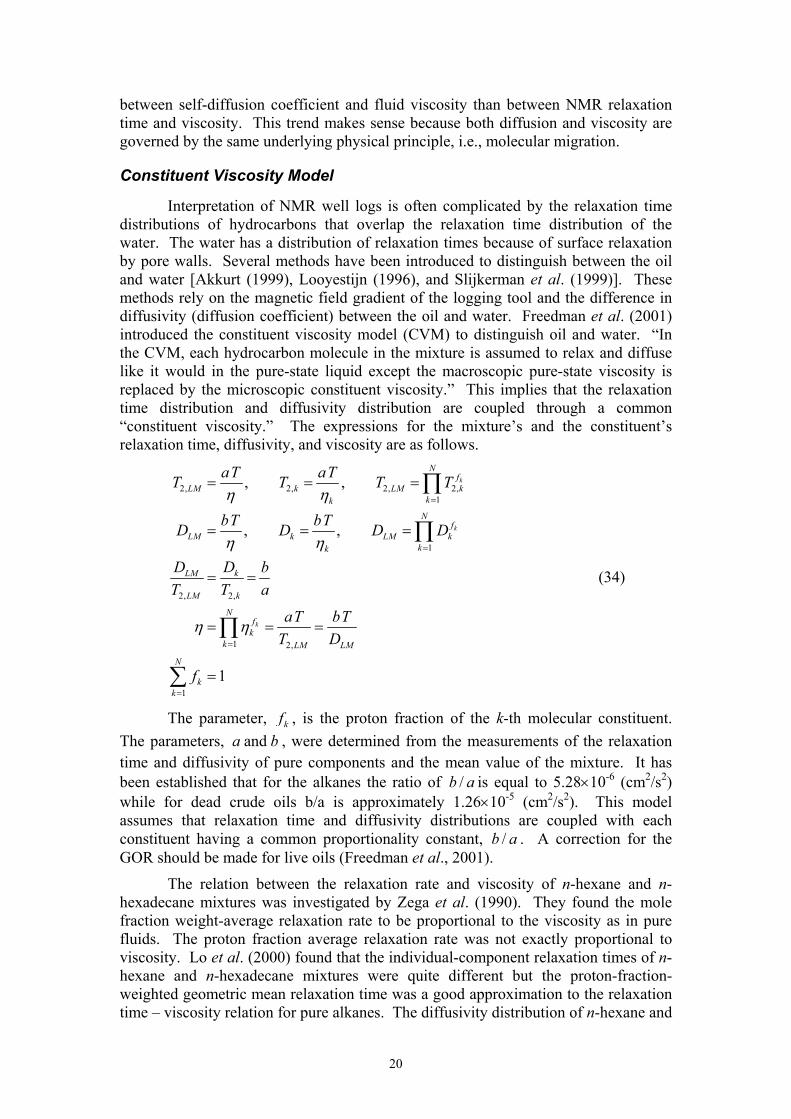
The viscosity and thus the relaxation time of heavy oils are very strongly dependent on the temperature. Thus measurements at different temperature is a good test of the correlation of T2,LM with the ratio of viscosity and temperature. Fig. 7 shows a plot of T2,LM as a function of the ratio of viscosity and temperature for measurements at 40°, 70°, and 100° C. These results show that the correlations which were developed for alkanes at close to ambient conditions apply to viscous, heated oils until T2,LM becomes close to the echo spacing of the measurement. It was mentioned earlier that short relaxation times are truncated by lack of data shorter than the echo spacing.

Live Crude Oils

Live oils differ from dead oils in that they contain dissolved gas components. Methane is the primary, but not the only, dissolved component. Supercritical methane and methane vapour relax by the spin-rotation mechanism. Cryogenic liquid methane relaxes by intermolecular dipolar coupling. With decreasing viscosity, the contribution from spin rotation to the relaxation process of methane successively increases and leads to an opposite trend for the relaxation time-viscosity relation compared to higher alkanes. In Fig. 8, the contributions to the proton relaxation time of methane are plotted as a function of viscosity divided by temperature. In gaseous methane, the relaxation time is mainly accounted for by spin-rotation. However, both dipolar and spin-rotation interactions become significant with increasing viscosity. In

9

cryogenic liquid methane, the relaxation mechanism is dominated by intermolecular dipolar coupling.

For formation fluids with a significant amount of solution gas, the relaxation behaviour will be governed by both dipolar interactions and spin rotation. The contribution from spin rotation increases with increasing gas-oil ratio and increasing hydrogen index of the gas phase. This is illustrated in Fig. 9, which includes methane-alkane mixtures, in addition to pure methane and pure higher alkanes.

Because of the opposite dependencies on the ratio of viscosity/temperature between dipolar interactions and spin rotation, prediction of the NMR relaxation times from PVT data for live oils is complicated. Generally speaking, live fluids will have shorter relaxation times than gas-free fluids of similar viscosity because of the additional contributions to the relaxation from spin rotation.

Figure 10 shows measured relaxation times for live reservoir fluids as a function of viscosity divided by temperature. Gas-free oils and oils with a relatively low solution gas-oil ratio are closely represented by the correlations developed for dead oils and alkanes. In contrast to this, the experimental data show that the relaxation times of oils with high solution gas-oil ratios are significantly shorter than those predicted by the correlations developed for gas-free systems. The measurements indicate that the difference between live oil data and the dead oil correlation can be greater factor of 2 for oils with solution gas-oil ratios larger than about 825 Scf/STB (standard cubic feet/stock tank barrel) (or 150 m3/m3) and can approach a factor of 5 for samples with as much as 2200 Scf/STB (or 400 m3/m3) solution gas oil ratios.

A comparison of the NMR response of live crude oils with those of live and dead oil-based mud filtrates (Fig. 11) illustrates that the relaxation times of both fluid types cover a similar range. Therefore, when approximating the relaxation spectra with a single relaxation time value, such as the logarithmic-mean value, it may be difficult to unambiguously distinguish between native oils and invaded oil-based mud filtrates. However, the measurements show that even live oil-based mud filtrates have a significantly narrower relaxation time distribution than those of live and dead crude oils. This effect should be exploited for downhole fluid identification (Prammer et al., 2001).

Lo et al. (1999) have shown that the relaxation times of methane-alkane mixtures show a significant deviation from the straight-line correlation for pure liquid alkanes. This departure is not exclusively due to the system being a mixture, since the log-mean relaxation of n-hexane and n-hexadecane mixtures followed the correlation for pure liquid alkanes. The deviation of the methane-alkane mixtures from the correlation for the liquid alkanes correlates with the methane content of the mixture or the gas/oil ratio, GOR, (in m3/m3) (Lo et al, 2000). The correlation of the measurements resulted in the following expression:

( ) ( )( ) ( ){ }

( ) ( )

10 1, 1 10

10 10 10

210 10

=Log / Log )

Log Log Log

0.127 Log 1.25Log 2.80

lineardeviation T T f GOR

deviation f GOR

GOR GOR

=

=

= − + −

(17)

10

The relaxation of the live oil can thus be estimated from the correlation in the absence of methane, denoted T1,linear, and the function of the GOR:

)(,1

1 GORfT

T linear= (18)

The correlation of the relaxation time as a function of viscosity/temperature and GOR is shown in Fig. 9. The contour lines of constant GOR are straight lines that are parallel to the line for dead oils.

The above correlation was developed from binary mixtures of methane and higher alkanes. Fig. 12 shows the deviation of live oil and OBM T2 relaxation time as a function of the GOR. The correlation of the deviation developed from methane-alkane measurements is shown for comparison.

Effect of Dissolved Oxygen

The previous section explained that molecular oxygen is paramagnetic and thus will contribute to the bulk relaxation of fluids even if it is present in small quantities. The effect of dissolved oxygen is best demonstrated by comparing the relaxation times of oils saturated with air with those of oils that have been degassed by freezing and vacuum. Measured relaxation time for alkanes from n-pentane to n-hexadecane are shown in Fig. 13. The relaxation time is clearly shorter for the samples that had not been degassed. The line in the figure is the correlation (Morriss et al., 1994) for crude oils that were not degassed. These results show that dissolved oxygen has the greatest effect for light oils and is nearly insignificant for n-hexadecane. Removal of oxygen is critical for measurements with hydrocarbon gases (Johnson and Waugh, 1961, Sandhu, 1966).

Air dissolved in water affects the bulk relaxation time of water. The measured relaxation time of air-saturated, deionized water at 30° C is in the range of 2-3 seconds. The measured T1 of carefully degassed, pure water at 30° C is 4.03 seconds (Krynicki, 1966).

Brine and Water-Based Drilling Fluids

Whole water-based drilling mud will have a short relaxation time because of the surface relaxation on the mud solids. If the mud filter cake is effective in filtering out the solids, the bulk fluid relaxation time of the filtrate is primarily a function of temperature and the dissolved components in the filtrate.

Drilling mud contains a number of additives that can affect the relaxation time of water. The effect of temperature on pure, degassed water is shown in Fig. 14. Figure 15 and 16 illustrate the effect of some additives.

When estimating the residual oil saturation, it is convenient to add a paramagnetic additive to make the relaxation time of water so short that it either will not be measured by the logging tool or is short enough to be distinguished from the oil signal. Horkowitz et al., 1997 added manganese chloride to the drilling fluid to "kill"

11

the water signal so that only oil was detected. MnCl2 could be used in that application because the formation was carbonate. Sandstone formations often have a significant amount of clay that can retard the propagation of manganese ions into the formation. Thus sandstone formations usually require the use of a chealated Mn-EDTA. The relaxation times as a function of concentration of these two forms of manganese ions are shown in Fig. 17.

Reservoir Gas

The primary component of natural gas is methane. Supercritical methane relaxes by the spin rotation mechanism and the relaxation time can be correlated with density and temperature. The relaxation time data of Gerritsma et al. (1970) and Lo (1999) are shown in Fig. 18.

The data of Gerritsma et al. are given along five isochors (constant density) and one isotherm. The data of Lo are at two temperatures and various pressures. The density corresponding to Lo’s conditions were calculated with the NIST program, SUPERTRAPP. The data were fitted by linear regression and the fit shown by the heavy line. Also shown are the correlations reported by Prammer et al. (1995) and Lo (1999). The correlation of Prammer appears to have been fitted to the data corresponding to the highest density. The correlation of Lo and the linear regression are hardly distinguishable. The correlations of T1 relaxation time with mass density and temperature are given by the following equations:

( )

( )

51

1.45

51

1.50

41

1.17

1.19 10 regression

1.57 10 Lo 1999

2.5 10 Prammer,et al. 1995

TT

TT

TT

ρ

ρ

ρ

×=

×=

×=

(19)

Although methane is usually the primary component of natural gas, other light hydrocarbons and non-hydrocarbons are usually present. Pure ethane and propane gas have relaxation times that are longer than that of methane, especially when correlated with molar density (Fig. 19).

A mixing rule can be developed for T1 in the gas mixtures with n components based on the kinetic model for spin rotation interaction (Bloom et al., 1967; Gordon, 1966). It is assumed that spin rotation interaction is dominant for all components in the mixture. For an n-component gas mixture, there may be n contributions to T1. The logarithmic mean T1 may be described as

ni fn

fi

f TTTT ,1,11,1logmean,11 ⋅⋅⋅⋅= , (20)

where fi is the resonant nucleus fraction of the i-th component in the mixture and T1,i is the individual relaxation time of the i-th component in the mixture.

12

The relaxation by the spin rotation interaction for the i-th component is caused by the collisions of the i-th molecule with various collision partners in the mixture. It has been empirically established that the contributions of various collision partners are additive (Jameson and Jameson, 1990; Jameson et al., 1987a; Jameson et al., 1991; Jameson et al., 1987b; Rajan and Lalita, 1975)

∑=

=

n

j i-jji

TT

1

11, ρ

ρ , (21)

where ρj is the partial molar density of the j-th component. In addition, Gordon has derived this additivity theoretically as a result of neglect of correlations between the effects of successive collisions and the assumption of binary collisions (Gordon, 1966). By assuming that all components have the inverse temperature to the 1.5 power, the coefficients for the interactions between like and unlike molecules can be estimated (Zhang et al., 2002).

5.11

TBT ij

ji

=

−ρ (22)

The coefficient Bij describes the interaction between probe molecule i and molecule j. Natural gas is composed primarily of methane. In addition, ethane, propane, CO2 and N2 are usually present. It is meaningful to calculate the coefficients Bij for various collision partners in natural gas. The coefficients Bij for the gas mixtures containing methane, ethane, propane, CO2 and N2 were calculated and summarized in Table 1. The details of the calculation can be found in (Zhang, 2002). The calculations for the pure components correspond to the dashed line in Figure 19.

Table 1: Values of the coefficients Bij for proton relaxation in the gas mixture of CH4, C2H6, C3H8, CO2, and N2

j CH4 C2H6 C3H8 CO2 N2

i

CH4 2.41×106 a

2.52×106 b

3.77×10

6 4.06×106 3.55×10

6 1.90×10

6

C2H6 1.06×107 1.58×10

7 1.66×10

7 1.45×107 8.02×10

6

C3H8 3.09×107 4.47×10

7 4.60×10

7 2.84×10

7 2.28×10

7

CO2 0 0 0 0 0 N2 0 0 0 0 0

a Estimated from experimental data of methane (Lo, 1999) b Calculated from the theoretical equation for spin rotation interaction using the molecular constants of methane

Carbon dioxide and nitrogen do not have protons but their presence in mixtures with methane results in a reduction of the relaxation time of methane compared to the correlation for pure methane based on mass density (Rajan et al., 1975). However, if the molar density rather than the mass density is used in the correlation, the methane relaxation in mixtures with CO2 or nitrogen will approximately correlate with that of pure methane. The symbols in Fig. 20 are the relaxation times of methane in mixtures with either CO2 or nitrogen compared with

13

the correlation for pure methane. The departure is apparently due to the collision cross-section of methane with these other gases being different from the methane-methane collision cross-section.

The dependence of the relaxation time of methane as a function of temperature and pressure (Kleinberg and Vinegar, 1996; Gerritsma et al., 1971) is shown in Fig. 21. It should be noted that the gas density was calculated for something slightly heavier than methane but it is unlikely that the contribution of any component other than methane to the relaxation time was included.

DIFFUSION

The subjects of viscosity and diffusion are parts of the general phenomena of transport in gases and liquids. Viscosity is concerned with momentum transport and governs both the motion of fluids and the motion of particles in a fluid under the influence of external forces (e.g. shear or gravitational forces). However, molecular migration can be observed even without the existence of external forces. This is the subject of Brownian motion, i.e. the statistical movement of atoms or molecules. Brownian motion has been extensively studied, beginning with the observations of random incessant motions of dust pollen in solution by Robert Brown in 1853. In the following section the basic principles of Brownian motion and its two major categories, diffusion and self-diffusion, will be explained.

Continuum Transport: Fick's Laws of Diffusion

The term diffusion describes the process of molecular transport within systems caused by the statistical movement of atoms or molecules. The relation between a concentration gradient a particle flux can be described with Fick's first law.

j Di i= − ∇ci (23)

The proportionality constant between the particle flux density, , and the concentration gradient, ∇ , is the diffusion coefficient, Di of the ith component of a mixture. Di is a unit of measurement of the velocity of molecular rearrangement.

jici

The time derivative of the concentration of a component i in a volume element has to be equal to the total flux of this component through the surface of the volume for conservation of particles.

ii

c jt

∂∂

= −∇i (24)

Combining the last two equations, Fick's second law

( )ii i

c D ct

∂∂

= ∇ ∇i (25)

describes the time derivative of the concentration for systems that are not in their equilibrium state. Generally speaking, the diffusion coefficient Di of a component is

14

also a function of its concentration. This process might be also referred to as mutual diffusion or transport diffusion.

Self-Diffusion

According to Fick’s first law, motion will always occur in systems that have a concentration gradient. However, particles move even without the existence of such a gradient. This process is called self-diffusion and is caused by the thermal energy of the particles. The self-diffusion coefficient Ds is a unit of measurement of the velocity of the Brownian movement under equilibrium conditions. Although no macroscopic particle fluxes are possible under such conditions, Fick's first and second laws can still be used to describe the process of self-diffusion. In this approach one assumes that a portion of the molecules are labeled, making it possible to observe their displacement within the system.

Diffusion Equation

In homogenous systems, the Brownian motion is determined by the coefficient of self-diffusion only. Since in such systems the self-diffusivity is independent of the spatial position of the molecules, Fick’s second law simplifies to

( ) 2,s

c r tD c

t∂

∂

∗∗= ∇

(26)

In this equation c* is the concentration of labeled molecules, and therefore the probability of finding a labeled particle in a certain position. The above equation is commonly referred to as the diffusion equation since the differential equation gives the probability of finding a molecule at time t at position r , if it initially was located at the position r . With the initial condition that the concentration of the labelled

molecules follows Dirac’s delta function, o

( ) ( )ro* ,c r r0 = −δ , the solution of the

diffusion equation is found to be a Gaussian distribution of the form

( )( )

( ) ( )2

00, 03

1, exp44

r rc r r t P r r t

DtDtπ∗

− = − =

,

(27)

This equation is commonly referred to as the propagator, (P r t), , or the fundamental solution of the diffusion equation since it allows the calculation of the mean square value of molecular displacement during the observation time, t:

( )r t P r t r dr D2 2 6( ) ,= =−∞

+∞

∫ t

(28)

The above relation is referred to as Einstein’s equation of diffusion and provides a straightforward definition of molecular diffusivity. In general, Einstein’s equation depends on the dimension, k, of molecular migration

15

x t y t z t k Dt2 2 2 2( ) ( ) ( )+ + = (29)

The expression above coincides with Einstein’s equation in isotropic systems where r t x t y t z t2 2 2 2( ) ( ) ( ) ( )= + + and the dimension of diffusion, k, is equal to

3.

The mean square displacement is thus found to be directly proportional to the total observation (or diffusion) time. Molecular propagation which follows this relation is generally called normal diffusion. Any confinements interfering with the diffusion process lead to a correlation of subsequent elementary jumps, and the direct proportionality between mean square displacement and diffusion time breaks down. This process is called anomalous diffusion or restricted diffusion. Depending on the nature of the confinement, different patterns of deviations from normal diffusion may be observed.

The single most important relation between viscosity and diffusion in liquids is the Stokes-Einstein equation. It has been found to be an accurate equation down to the molecular length scale and it finds wide application in relating molecular diffusion to fluid viscosity.

00

(0) ( )6

Bk TD U U t dtRπη

∞

≡ =∫ (30)

According to the Stokes-Einstein equation, the self-diffusivity D0 is defined via the velocity autocorrelation function, <U(0)U(t)>, and is related to the thermal energy, kBT, and the viscous drag on a sphere of radius R.

Measurement Techniques - Diffusion and Self-Diffusion

Diffusion Measurements

In systems that are not in their equilibrium state, concentration gradients lead to particle fluxes that can be observed macroscopically. According to Fick's first law, a determination of the diffusion coefficient of a certain species of molecules can be based either on measurements of both the flux density and the gradients of the concentration or on measurements of the particle distribution at different times.

Molecular concentrations can be determined by chemical as well as various physical methods, since numerous properties such as weight, refraction index, birefringence, radioactivity, spectral absorbance, and transmittance depend on the composition of the system. Consequently, a wide variety of experimental techniques for determining the diffusion coefficient of systems have been developed.

Self-Diffusion Measurements by NMR As an alternative to the tracer techniques, there are several methods that allow the direct observation of the diffusion path, i.e., the mean square displacement of the random walk of the diffusing molecules. Based on Einstein’s equation, the coefficient of molecular diffusion can be calculated knowing the mean square displacement of

16

the particles within a given diffusion time. However, the displacements of the molecules must be much larger than the mean length of the elementary steps of diffusion. Nuclear Magnetic Resonance Pulsed Field Gradient Technique ("PFG NMR") is currently the only method that gives a direct measurement of molecular displacements over such large distances. Unfortunately, current NMR logging tools are not capable of performing PFG NMR measurements. However, diffusion, self-diffusion, and fluid flow can also be indirectly determined from relaxation measurements in a static field gradient.

Pulsed Field Gradient NMR (PFG NMR) The principle of measuring molecular diffusivity using PFG NMR is that the

spatial position of each spin (and hence, each molecule) is marked by its specific Larmor frequency within a spatially inhomogenous magnetic field. PFG NMR spectrometers are equipped with additional coils that create a switchable, well-defined magnetic field. This additional magnetic field is often referred to as the ‘magnetic field gradient’ because it creates a gradient of the effective magnetic field over the sensed volume when superimposed onto the background magnetic field. Since the Larmor frequency of precessing spins is directly proportional to the magnetic flux density effective at the position of the respective spin, a magnetic field gradient over the sensed volume will result in a variation of the Larmor frequency and tag the position of each magnetic moment with respect to the direction of the magnetic field gradient.

Experimentally, during the radio frequency (RF) pulse sequence used to create a spin echo (like the Hahn, or the stimulated echo sequence), the magnetic field gradient pulses are switched on for a short duration (typically up to a few milliseconds). The sequence of RF- and magnetic field gradient pulses is chosen such that the variation of the Larmor frequency brought about by an individual field gradient pulse is exactly compensated for by a subsequent field gradient pulse if the spins have not changed their positions during the time interval between the two gradient pulses. However, if the spins have moved, a net variation of the Larmor frequency will remain after all RF- and magnetic field gradient pulses have been applied. Therefore, diffusion of spins will result in a measurable attenuation of the NMR signal. The effect is proportional to the intensity of the magnetic field gradient pulses, g, duration, δ, the diffusion time (time between subsequent field gradient pulses), ∆, and the self-diffusion coefficient of the molecules, D (Stejskal and Tanner, 1965):

(( 2 2 2

0

exp / 3 .M g DM

ψ γ δ δ= = − ∆ − )) (31)

The spin-echo attenuation, Ψ, is the ratio of the amplitudes of the spin echoes with and without the application of magnetic field gradient pulses, M and M0, respectively. In this way, additional attenuation of the spin echoes due to relaxation processes during the diffusion time will be cancelled out. During a PFG NMR experiment, the amplitude of spin echoes is measured as a function of the area of the field gradient pulses, g×δ, at a given diffusion time. The slope of this echo attenuation curve is proportional to the self-diffusion coefficient.

It has been shown (Mitra, 1992; Fleischer, 1994; Cowan, 1997) that the PFG NMR experiment can be interpreted in terms of a generalized scattering experiment. This approach implies the possibility of defining a "generalized wave vector"

17

, γ δ=k g , and, therefore, of determining the space scale probed in the experiment. Using the strong field gradients of the stray field of a cryomagnet, the NMR field gradient technique can provide a maximum spatial resolution of about 100 Å. Since the accessible diffusion times can vary between milliseconds up to seconds, a broad range of diffusion coefficients can be determined. Hence, it is possible to apply PFG NMR to determine the diffusivity of gases and liquids, including crude oils.

Self-Diffusion Measurements by CPMG with Constant Magnetic Field Gradients.

Current NMR logging tools are not equipped with switchable magnetic field gradients. However, information about fluid diffusivity can be obtained with the static field gradient of the logging tool and changing the echo spacing. The underlying concept is that the NMR response for fluids confined to the pore space is given by:

( )

11 1, 1, 1,

2

22 2, 2, 2, 2,

1 1 1 1 ,

1 1 1 1 1 .12

bulk surface bulk

bulk surface diffusion bulk

ST T T T V

gTE DST T T T T V

ρ

γρ

= + = +

= + + = + +

(32)

In these equations, the pore fluid has a diffusion coefficient, D, and is confined to pores with a surface-to-volume ratio, S/V. The surfaces of these pores have a surface relaxivity of ρ, which is effective either for the longitudinal or the transverse relaxation process, 1ρ and 2ρ , respectively. The transverse relaxation time is measured with a CPMG pulse sequence using an inter-echo spacing, TE, and a constant magnetic field gradient, g. γ is the proton gyromagnetic ratio.

Based on the above equations, it is possible to calculate an averaged diffusion coefficient of the pore fluids. However, several assumptions need to be fulfilled:

One approach is to measure both the T1 and T2 of the system and look for the difference. The relaxation times T1 and T2 for the bulk fluids must be equal, i.e., the NMR relaxation must be governed by the motional narrowing process. In order to cancel surface relaxation effects, the surface relaxivities for both the T1 and the T2 relaxation process also need to be equal. Naturally, there is no contribution from surface relaxation if bulk fluids are measured under laboratory conditions.

Under these assumptions, a clear difference between the measured T1 and T2 relaxation times will be observed if the diffusion term dominates the relaxation response. That is generally the case only for fluids with low viscosities (which also satisfy the motional narrowing requirement), measured as a bulk sample or as a non-wetting phase. An additional complication is that the calculated diffusion coefficient is an ‘apparent’ diffusivity. The difference between T1 and T2 does not reveal whether the diffusion has become restricted because the propagation of molecules has been hindered by the geometry of the pore network.

Alternatively, the estimation of the diffusion coefficient of the pore fluids can be based on T2 measurements only. If the transverse relaxation time is measured with a CPMG technique at various inter-echo spacings, TE, the diffusivity of the fluids can be calculated from the observed shift of the relaxation spectra towards shorter relaxation times with increasing TE’s. Similar to the T1/T2 method mentioned above,

18

this approach will only work if the relaxation response is dominated by the diffusion term. Experimentally, the available range of inter-echo spacings, and, therefore, detectable diffusion coefficients is limited. Finally, it has to be verified that the calculated relaxation time distribution is not shifted because of different sampling interval with the change in echo spacing, even in the absence of any field gradients. The recently introduced, “diffusion editing” sequence (Hurlimann et al., 2002, Prammer et al., 2002)) partially overcomes this limitation by using variable duration echo spacing only for the first echo and using short echo spacing for the subsequent echos.

Self Diffusion of Hydrocarbon Systems

The self-diffusion coefficient of super critical methane correlated as a function of density and temperature is shown in Fig. 22. The data shown here is correlated with data in the range of 273° to 454° K. The temperature dependence is correlated with temperature raised to the inverse 0.7 power. The exponent was reported to range from 0.6 to 0.9 for data that included saturated vapor along the coexistence curve (Oosting and Trappeniers, 1971; Harris, 1978). The inverse square root temperature dependence is appropriate for a smooth hard sphere fluid in the low-density limit (Reid, Prasunitz, and Poling, 1987, pg. 595-6). The correlation curve in Fig. 22 is fitted to a quadratic function of density.

60.710 2.64 1.26 11D

T2ρ ρ ρ= + − (33)

where ρ is the density in g/cm3, D is the diffusion coefficient in cm2/s, and T is the temperature in K. The Chapman-Enskog theory predicts that the curve should have a zero slope as density approaches zero. A plot of the methane diffusion coefficient as a function of pressure and temperature is shown in Fig. 23 (Kleinberg and Vinegar, 1996).

The self-diffusion coefficients of alkanes, including methane, ethane, propane, and mixtures of methane and higher alkanes, are shown as a function of viscosity/temperature in Fig. 24. The correlation indicates that the Stokes-Einstein relationship is followed. The relaxation time is shown as a function of the self-diffusion coefficient in Fig. 25. While the self-diffusion coefficient and relaxation time are proportional for the higher alkanes, methane, ethane, propane and mixtures of methane with higher alkanes depart from the linear relationship because methane relaxes by the spin-rotation mechanism, even when dissolved in the liquid phase.

Figure 26 shows the distribution of self-diffusion coefficients for a 33º API live crude oil with about 825 Scf/STB dissolved gas. Similar to their relaxation response, crude oils have a broad distribution of diffusivities compared to that of pure alkanes. While the diffusivity of a gas-free system is relatively insensitive to pressure, a clear shift of the diffusion coefficient towards smaller values with increasing pressure can be observed for the live oil. This trend is also illustrated in Fig. 27, which also compares the diffusion coefficients of live oils with those at ambient conditions after the solution gas has been depleted.

Figure 28 shows the diffusivities of various live and dead oils and oil-based mud filtrates as a function of fluid viscosity. The diagram also illustrates the correlation that has been developed from measurements on pure higher alkanes and dead crude oils. Experiments have shown that live oils have a better correlation

19

between self-diffusion coefficient and fluid viscosity than between NMR relaxation time and viscosity. This trend makes sense because both diffusion and viscosity are governed by the same underlying physical principle, i.e., molecular migration.

Constituent Viscosity Model

Interpretation of NMR well logs is often complicated by the relaxation time distributions of hydrocarbons that overlap the relaxation time distribution of the water. The water has a distribution of relaxation times because of surface relaxation by pore walls. Several methods have been introduced to distinguish between the oil and water [Akkurt (1999), Looyestijn (1996), and Slijkerman et al. (1999)]. These methods rely on the magnetic field gradient of the logging tool and the difference in diffusivity (diffusion coefficient) between the oil and water. Freedman et al. (2001) introduced the constituent viscosity model (CVM) to distinguish oil and water. “In the CVM, each hydrocarbon molecule in the mixture is assumed to relax and diffuse like it would in the pure-state liquid except the macroscopic pure-state viscosity is replaced by the microscopic constituent viscosity.” This implies that the relaxation time distribution and diffusivity distribution are coupled through a common “constituent viscosity.” The expressions for the mixture’s and the constituent’s relaxation time, diffusivity, and viscosity are as follows.

2, 2, 2, 2,1

1

2, 2,

1 2,

1

, ,

, ,

1

k

k

k

Nf

LM k LM kkk

Nf

LM k LM kkk

kLM

LM k

Nf

kk LM LM

N

kk

aT aTT T T

bT bTD D D

DD bT T a

aT bTT D

f

η η

η η

η η

=

=

=

=

= = =

= = =

= =

= = =

=

T

D

∏

∏

∏

∑

(34)

The parameter, kf , is the proton fraction of the k-th molecular constituent. The parameters, , were determined from the measurements of the relaxation time and diffusivity of pure components and the mean value of the mixture. It has been established that for the alkanes the ratio of b is equal to 5.28×10

anda b

/ a -6 (cm2/s2) while for dead crude oils b/a is approximately 1.26×10-5 (cm2/s2). This model assumes that relaxation time and diffusivity distributions are coupled with each constituent having a common proportionality constant, b . A correction for the GOR should be made for live oils (Freedman et al., 2001).

/ a

The relation between the relaxation rate and viscosity of n-hexane and n-hexadecane mixtures was investigated by Zega et al. (1990). They found the mole fraction weight-average relaxation rate to be proportional to the viscosity as in pure fluids. The proton fraction average relaxation rate was not exactly proportional to viscosity. Lo et al. (2000) found that the individual-component relaxation times of n-hexane and n-hexadecane mixtures were quite different but the proton-fraction-weighted geometric mean relaxation time was a good approximation to the relaxation time – viscosity relation for pure alkanes. The diffusivity distribution of n-hexane and

20

n-hexadecane mixtures overlapped too much to determine if the diffusivity distribution corresponded to the relaxation time distribution. Freedman et al. (2001) studied mixtures of n-hexane (C6H14) and squalene (C30H50) and demonstrated the relation between the relaxation time and diffusivity distributions for these mixtures.

The relaxation time and diffusivity distributions are shown in Figs. 29 and 30, respectively, and are summarized in Table 2. The values in the tables are the bi-exponential fit results. The light vertical line on each plot is the relaxation time estimated by fitting the CPMG response to a bi-exponential model. H(C6) is the proton fraction of hexane in the mixture. A(C6) is the fraction of the area attributed to hexane. There is good agreement between H(C6) and A(C6). The peaks of the diffusivity distributions are broader than those of the T2 distributions. This can be explained by the difference in signal/noise for the two measurements. Figure 31 plots constituent and log mean relaxation time and diffusivity as function of composition. There is about an order of magnitude change in the relaxation time and diffusivity of squalene. The change for n-hexane is less. Figure 32 is a plot of the ratio of diffusivity and relaxation time for squalene and n-hexane. The dashed line is the ratio, , determined for pure and mixtures of alkanes. The average absolute deviation of the ratio, D/T

/b a2, from the independently determined value of is 27%.

It is clear that the deviation could be reduced if was determined specifically for the n-hexane and squalene mixture. Figure 33 is the correlation between the pure and constituent diffusivity and relaxation time for the n-hexane and squalene systems. The measured points compare well with the correlation that was independently developed from pure alkanes and mixture of alkanes.

/b a/b a

Table 2 Relaxation time and diffusivity of n-hexane and squalene mixtures

H(C6) T2(C6), s T2(C30), s D(C6), cm2/s D(C30), cm2/s

0.00 0.294 1.01E-06

0.38 4.59 0.90 1.27E-05 3.47E-06

0.50 5.75 1.18 1.70E-05 4.94E-06

0.69 7.52 1.69 3.02E-05 9.89E-06

1.00 9.78 4.60E-05

The measurements of relaxation time and diffusivity for the pure materials and mixtures of n-hexane and squalene verify the coupling between the relaxation time and diffusivity of constituents in a mixture. The area fractions in the distributions correspond to the proton fraction of the corresponding constituent.

HYDROGEN INDEX

Definition of Hydrogen Index

The amplitude of the response of the NMR logging tool is calibrated with respect to that of bulk water at standard conditions. Thus the amplitude of the magnetization before attenuation by relaxation processes, M0, is expressed as:

21

(0 w w o o g g )M S HI S HI S HIφ∝ + + (35)

where φ is the porosity, Sp is the saturation of phase p, and HIp is the hydrogen index of phase p, where p = brine, oil, or gas. The HI is defined as follows,

3

Amount of hydrogen in sampleAmount of hydrogen in pure water at STPmoles H/cm

0.111/

0.111m H

HI

N Mρ

≡

=

=

(36)

where mρ is the mass density of the fluid in g/cm3 , NH is the number of hydrogen in the molecule, and M is the molecular weight. The denominator of the last expression, 0.111, is the moles of hydrogen in one cubic centimeter of water at standard conditions. The numerator is the number of moles of hydrogen in the same volume of the bulk sample at the conditions of the measurement.

The HI of a fluid sample can be measured in the laboratory by measuring the response of the sample of known volume at the conditions of interest:

( )( )2 2

, at conditions of interest

, at standard conditions

/

/o fluid fluid

o H O H O

M VHI

M V= (37)

M0 can be determined either by the extrapolation of a CPMG or FID response to zero time to recover any signal losses that might have occurred during the dead time of the spectrometer. Alternatively, the cumulative distribution of relaxation times after inverting the measured signal decay can be used to determine M0. However, when using the latter procedure, errors brought about by oscillations in the early echoes might be harder to detect.

20,H OM is the respective magnetization of water at standard conditions. When determining the HI experimentally, the decreasing sensitivity of the spectrometer with increasing temperature according to Curie- and Boltzmann effects needs to be considered.

HI of Brines

Recall that the HI is relative to pure water at ambient conditions. Thus brine that contains a large quantity of salts may have a HI that deviates significantly from unity (Fig. 34).

22

HI of Gas

The HI of gas mixtures can be determined by extending the definition of HI:

( )

3

,

,

moles H/cm0.111

, for single component0.111

, for mixture0.111

moles/liter0.111 0.111 111

H

n

i H ii

n

i H iHi H

HI

N

N

y N NN

ρ

ρ

ρ ρρ

=

=

=

= = =

∑

∑

(38)

where , iρ ρ and ρ , are molar density, partial molar density, and average molar density, respectively. The final expression has the density expressed as moles/liter, the units commonly used in PVT calculations. , and ,,i Hy N i HN are mole fraction, number of hydrogen per molecule of component i, and the average moles of hydrogen per mole of mixture, respectively . Table 3 is an example calculation for the average moles of hydrogen for a typical separator gas.

The HI of the gas can be computed by multiplying the molar density from PVT calculations with the average number of hydrogen per molecule, Fig. 35.

Table 3. Example calculation for the average moles of hydrogen in a mole of a typical separator gas mixture Component Mole fraction, iy ,H iN Carbon dioxide 0.0167 0 Nitrogen 0.0032 0 Methane 0.7102 4 Ethane 0.1574 6 Propane 0.0751 8 i-Butane 0.0089 10 n-Butane 0.0194 10 i-Pentane 0.0034 12 n-Pentane 0.0027 12 Hexanes 0.0027 14 Heptanes plus 0.0003 16 Total or average 1.0000 4.785

Correlations for Hydrogen Index

Gaymard and Poupon (1968) introduced a correlation of HI for hydrocarbons as a function of the mass density. Their correlation is based on the assumption that the hydrocarbons can be represented by alkanes.

23

( )[ ]29.02.015.09 mmHI ρρ −+= (39)

Vinegar et al. (1991) and Kleinberg and Vinegar (1996) introduced a correlation based on the measurements of stock tank crude oils at ambient conditions. Their correlation has the HI equal to unity for oils lighter than 25º API and decreasing for heavier oils. These two correlations are illustrated in Fig. 36 along with the calculated HI for some pure hydrocarbons at ambient conditions and methane at elevated pressures.

Figure 36 shows that the correlation of Gaymard and Poupon is satisfactory for methane at high pressures and for the pure liquid alkanes at ambient conditions. Thus one can expect that the correlation will also be satisfactory for the gas phase or methane dissolved in a liquid phase containing only higher alkanes, such as gas condensate. The correlation of Kleinberg and Vinegar appears to capture the reduction in HI that is observed for aromatic or polyaromatic hydrocarbons. However, the correlation is for stock tank oil and thus may not adequately represent live oils with a high GOR.

HI of Heavy Oils

LaTorraca et al. (1999, 2000) pointed out that the measured HI values of heavy crude oils may be less than actual values because of information lost due to finite echo spacing time. Thus the authors defined an apparent HI that depends on the inter-echo spacing and emphasized that the HI of heavy oil should be measured at the same echo spacing as the logging tool if the information is to be used to interpret logs. They also claim that the actual HI, based on geochemical analysis, should be within 5% of unity. While the apparent HI can be used to estimate the viscosity of the heavy oil, measurements of the HI of crude oils and pure hydrocarbons have shown that samples with T2 much greater than the echo spacing had measured HI of about 0.9, Fig. 37. Also, 1-methylnaphthlene and toluene, both of which have T2 greater than 1 second, have measured HI less than 0.7. Mirotchnik et al. (1999) demonstrated the increase in apparent HI with increased temperature for bitumen. Increasing temperature shifted the T2 distribution towards longer times, and more of the distribution could be measured for a given echo spacing.

HI for Hydrocarbon Mixtures and Live Oils

The HI of live oils, i.e., oils with a certain amount of solution gas, can significantly deviate from unity. Although live oils often occur as undersaturated oils, a significant amount of solution gas can be dissolved in the oil phase especially in high temperature, high pressure reservoirs. As a result, the density of the formation fluid is reduced while thermal expansion coefficients and compressibility are increased compared to stock tank conditions. Therefore, the HI of live oils are reduced and more pressure-dependent than those of gas-free oils.

When representative samples of the formation fluids have been preserved, the measurement of their NMR response at reservoir conditions can significantly reduce the uncertainty in the interpretation of wireline NMR data. The correct determination

24

of the HI of the hydrocarbon phase directly impacts crucial reservoir parameters such as porosity and hydrocarbon saturation. Indirectly, uncertainties in the estimation of the HI are carried forward to the calculation of formation permeability based on NMR logging data since the ratio of bound- and free fluids also depends on the HI. Figure 38 illustrates the impact of wrongly determined HI on the calculation of porosity and permeability. Since typically only movable hydrocarbons show HI smaller than unity, the error is increased for smaller ratios of bound fluids to total porosity. This calculation is based on the assumption that the error in hydrogen index determination affects all movable fluids. This situation represents the NMR measurements acquired in an undrained reservoir well above the transition zone.

Experimentally, the hydrogen index of live oils can be measured by comparing their NMR response to that of water at standard conditions. The experimental setup needs to address the decreased sensitivity of the spectrometer with increasing temperature. Care needs to be taken to ensure that the formation fluid can be transferred from a pressurized storage cylinder to the NMR probe without falling below either the bubble point or the onset pressure of asphaltene precipitation. The pressurized fluid sample needs to be carefully equalized prior to the NMR measurement to ensure that no changes in the chemical composition have occurred.

Figure 39 illustrates the results of the HI measurements on live oils and mixtures of oil-based mud filtrates and methane at various conditions. Gas-free oil-based mud filtrates have HI very close to unity. With increasing GOR, the HI continuously decreases, related to changes in fluid density. The lowest values of around 0.8 were obtained for undersaturated oils with solution gas-oil ratios of about 2000 Scf/STB. If a 25% porosity formation was saturated to 80% with this oil, and an HI of unity was wrongly assumed in the interpretation of NMR log data, the NMR-determined porosity of this formation would be undercalled by about 4 porosity units.

Calculation of the HI of Live Oils The HI of a hydrocarbon mixture can be calculated exactly from the mass

density and hydrogen: carbon ratio (H:C), R, if contributions to the NMR signal arising from the hydrogenated compounds of heteroatoms, like sulphur compounds (mercaptans or thiols) or oxygen compounds (organic acids in immature crude oils) can be neglected. (Zhang et al., 1998)

( )[ ]111.0

008.1011.12 RRHI m +

=ρ

(40)

This formula is convenient for pure hydrocarbons or mixtures for which the density and R can be determined. However, H:C is generally not known for crude oils and complete geochemical analysis might not always be available. Because there are only three parameters in the above relation, the value of R can be determined for a stock tank oil if the HI and density are measured at ambient conditions.

STOSTOm

STOSTO HI

HIR

112.0333.1

, −=

ρ (41)

25

If one has the usual PVT data, the mass density and R can be determined for the live oil. A PVT report expresses the volumetric data and composition such as the oil formation volume factor, Bo, and the solution gas:oil ratio, Rs, as a function of pressure at reservoir temperature.

The mass density can be determined as follows,

,,

0 0

0.178 s m gasm STOm

RB B

ρρρ = + (42)

Here Rs has the units of Scf/STB and ,m gasρ is the gas density at standard conditions. The H:C for a live oil can be determined with the following formula.

( )( )

( )( )

11.90.178

11.911.9

1 0.17811.9

gas s gas STOSTO

STO gas

s gas STO

STO gas

R R RR

RR

R RR

ρρρ

ρ

++

+=

++

+

(43)

The composition of the separator gas yields its H:C ratio, Rgas. As a result, the HI of the live oil can be calculated using the mass density and H:C ratio determined from the previous two equations.

The HI of two live GOM crude oils were calculated at reservoir conditions. One is a 30º API crude oil with a solution gas/oil ratio of 749 Scf/STB at a bubble point pressure of 4150 psia. The other is a 38º API gravity crude oil with a solution gas/oil ratio of 1720 Scf/STB at a bubble point pressure of 4575 psia. The results are shown in Fig. 40 along with the G&P and K&V correlations.

At stock tank oil condition, the HI value of the 30º API crude oil is 0.959, which is close to the default value of unity. However, when pressure increases, more gas (mostly methane) dissolves in the crude oil, causing decreasing density and increasing H:C ratio. When pressure reaches the bubble point pressure, HI reduces to the lowest value of 0.857. As pressure continues to increase above bubble point, no more gas dissolves in the crude oil, but instead the oil is compressed. Since the composition does not change, the H:C ratio of the reservoir fluid remains constant. HI then linearly increases with increasing density above the bubble point. The 38º API crude oil has a HI of 0.983 at stock tank conditions but the HI reduces to about 0.806 at the bubble point pressure of 4575 psi. The higher solution gas/oil ratio of the 38º API crude causes its HI to deviate from unity more significantly than for the 30º API crude. Both oils show significant deviation from the G&P and K&V correlations.

ACKNOWLEGMENT One of the authors (GJH) acknowledges the financial support of NSF, USDOE, and a consortium consisting of Arco, Baker Atlas, Chevron, Exxon-Mobil, Halliburton-NUMAR, Kerr McGee, Marathon, Norsk Hydro, Phillips, PTS, Saga, Schlumberger, and Shell. Also, the contributions of S.-W. Lo, Q. Zhang, Y. Zhang, W.V. House, and R. Kobayashi are recognized.

26

REFERENCES Akkurt, R., Vinegar, H.J., Tutunjian, P.N., and Guillory, A.J.: “NMR Logging of

Natural Gas Reservoirs,” The Log Analyst (1996), November-December, 33-42.

Appel, M., Freeman, J.J., Perkins, R.B., and van Dijk, N.P.: “Reservoir Fluid Study by Nuclear Magnetic Resonance,” paper HH, SPWLA 41st Annual Logging Symposium, (4-7 June, 2000) Dallas, TX.

Benedek, G.B. and Purcell, E.M.: “Nuclear Magnetic Resonance in Liquids under High Pressure,” J. Chem. Phys. (1954), 22.12, 2003-2012.

Bloembergen, N., Purcell, E.M., and Pound, R.V.: “Relaxation Effects in Nuclear Magnetic Resonance Adsorption,” Phys. Rev. (1948), 73.7, 679-712.

Bloom, M., Bridges, F., and Hardy, W. N., 1967, Nuclear Spin Relaxation in Gaseous Methane and Its Deuterated Modifications: Canadian Journal of Physics, v. 45, p. 3533-3554.

Bouton, J., Prammer, M.G., Masak, P., and Menger, S.: “Assessment of Sample Contamination by Downhole NMR Fluid Analysis,” SPE 71714 presented at the 2001 SPE ATCE, New Orleans, LA, 30 September- 3 October.

Cowan, B.: Nuclear Magnetic Resonance and Relaxation, Cambridge University Press (1997), New York, NY.

Dawson, R., Khoury, F., and Kobayashi, R.: “Self-Diffusion Measurements in Methane by Pulsed Nuclear Magnetic Resonance,” AIChE J.(1970), 16.5, 725-729.

Fleischer, G., and Fujara, F. (1994), in P. Diehl, E. Fluck, H. Gunther, R. Kosfeld, J. Seelig (Eds.), NMR Basic Principles and Progress, Vol 30, Berlin: Springer Verlag.

Freedman, R., Lo, S.-W., Flaum, M., Hirasaki, G.J., Matteson, Sezginer, A.: “A New NMR Method of Fluid Characterization in Reservoir Rocks: Experimental Confirmation and Simulation Results,” SPEJ (December 2001) 452-464.

Freedman, R., Heaton, N., and Flaum, M.: “Field Application of a New Nuclear Magnetic Resonance Fluid Characterization Method” SPE 71713 presented at the 2001 APE ATCE, New Orleans, LA (Sept. 30 – Oct. 3, 2001)

Gerritsma, C.J. and Trappeniers, N.J.: “Proton-Spin-Lattice Relaxation and Self-Diffusion in Methanes I. Spin-Echo Spectrometer and Preparation of the Methane Samples,” Physica (1971) 51, 365-380.

Gerritsma, C.J., Oosting, P.H., and Trappeniers, N.J.: “Proton-Spin-Lattice Relaxation and Self-Diffusion in Methanes II. Experimental Results for Proton Spin-Lattice Relaxation Times,” Physica (1971) 51, 381-394.

Gordon, R.G.: “Kinetic Theory of Nuclear Spin Relaxation in Gases,” J. Chem. Phys. (1966) 14.1, 228-234.

Greiner-Schmid, A., Wappmann, S, Has, M., and Ludemann, H.-D.: “Self-diffusion in the compressed fluid lower alkanes: Methane, ethane, and propane,” J. Chem. Phys. (1991) 94.9, 5643-5649.

27

Harris, K.R.: “The Density Dependence of the Self-Diffusion Coefficient of Methane at –50, 25 and 50 C,” Physica (1978), 94A, 448-464.

Hennel, J.W. and Klinowski, J.: Fundamentals of Nuclear Magnetic Resonance, Longman Scientific & Technical (1993) Essex, England.

Horkowitz, J.P., Vinegar, H.J., Hartman, D.E., Coates, G.R., and Clerke, E.A.: “Residual Oil Saturation Measurements In Carbonates With Pulsed NMR Logs,” paper Q, SPWLA 36th Annual Logging Symposium, (26-29 June, 1995) Paris, France.

Hubbard, P. S., “Theory of Nuclear Magnetic Relaxation by Spin-Rotational Interactions in Liquids”, Phys. Rev. (1963), 131, 1155-1165.

Hubbard, P.S.: “Nuclear Magnetic Relaxation by Intermolecular Dipole-Dipole Interactions,” Phys. Rev. (1963) 131, 275-282.

Hurlimann, M.D., Venkatarmanan, L., Flaum, C., Speier, P., Karmonik, C., Freedman, R., and Heaton, N.: “Diffusion Editing: New NMR Measurement of Saturation and Pore Geometry,” paper FFF presented at the SPWLA 43rd Annual Logging Symposium, Oiso, Japan, (June 2-5, 2002).

Jameson, C. J., Jameson, A. K., and Smith, N. C., 1987a, 15N Spin-Relaxation Studies of N2 in Buffer Gases. Cross Sections for Molecular Reorientation and Rotational Energy Transfer: The Journal of Chemical Physics, v. 86, p. 6833-6838.

Jameson, C. J., Jameson, A. K., Smith, N. C., Hwang, J. K., and Zia, T., 1991, 13C and 1H Spin Relaxation in CH4 in the Gas Phase: The Journal of Physical Chemistry, v. 95, p. 1092-1098.

Jameson, C. J., Jameson, A. K., Smith, N. C., and Jackowski, K., 1987b, Cross Sections for Transfer of Rotational Angular Momentum in CO2 from 13C Spin Relaxation Studies in the Gas Phase: The Journal of Chemical Physics, v. 86, p. 2717-2722.

Johnson, C.S. and Waugh, J.S.: “Nuclear Relaxation in Gases: Mixtures of Methane and Oxygen,” J. Chem. Phys. (1961), 35.6, 2020-2024.

Kashaev, S.Kh.G, Le, B., and Zinyatov, M.Z.: “Proton Spin-Lattice Relaxation, Viscosity, and Vibration of Molecules in the Series of n-Paraffins,” translated from Doklady Akademii Nauk SSSR, 157.6, 1438-1440 (August, 1964) 846-848.

Kleinberg, R.L. and Vinegar, H.J.: “NMR Properties of Reservoir Fluids,” The Log Analyst (1996), November-December, 20-32.

Krynicki, K.: “Proton Spin-Lattice Relaxation in Pure Water between 0°C and 100°C,” Physica (1966), 32, 167-178.

LaTorraca, G.A., Stonard, S.W., Webber, P.R., Carlson, R.M., and Dunn, K.J.: “Heavy Oil Viscosity Determination using NMR Logs,” paper PPP, SPWLA 40th Annual Logging Symposium, (30 May – 3 June, 1999), Oslo, Norway.

LaTorraca, G.A., Dunn, K.J., Webber, P.R., and Carlson, R.M.: “Low-Field NMR Determination of the Properties of Heavy Oils and Water-in Oil Emulsions,” Magnetic Resonance Imaging (1998) 16, 5/6, 659-662.

28

Lo, S.-W., Hirasaki, G.J., House, W.V., Kobayashi, R.: “Mixing Rules and Correlations of NMR Relaxation Time with Viscosity, Diffusivity, and Gas/Oil Ratio of Methane/Hydrocarbon Mixtures,” SPE 63217 presented at the 2000 SPE ATCE, (1-4 October, 2000), Dallas, TX.

Lo, S.-W.: Correlations of NMR Relaxation Time with Viscosity/Temperature, Diffusion Coefficient and Gas/Oil Ratio of Methane-Hydrocarbon Mixtures, (1999) Ph.D. thesis, Rice University, Houston, TX.

McConnell, J., The Theory of Nuclear Magnetic Relaxation in Liquids, Cambridge University Press, New York, 1987.

Mirotchnik, K.D., Allsopp, K., Kantzas, A., Curwen, D., and Badry, R.: “Low Field NMR-Tool for Bitumen Sands Characterization: A New Approach,” SPE 56764 presented at the 1999 SPE ATCE, Houston, TX, 3-6 October.

Mitra, P.P., Sen, N.S., Schwartz, L.M., and Le Doussal, P.: “Diffusion Propagator as a Probe of the Structure of Porous Media,” Phys. Rev. Lett. (1992), Vol. 68, No. 24, 3555-3558.

Morriss, C.E., Freedman, R., Straley, C., Johnston, M., Vinegar, H.J., and Tutunjian, P.N.: “Hydrocarbon Saturation and Viscosity Estimation from NMR Logging in the Belridge Diatomite,” The Log Analyst (1997), March-April, 44-59.

Muller, B.H. and Nobel, J.D.: “Proton Spin-Lattice Relaxation in Pure Liquid Ethane and Some of Its Duterated Modifications,” (not complete)

Oosting, P.H. and Trappeniers, N.J.: “Proton-Spin-Lattice Relaxation and Self-Diffusion in Methanes III Interpretation of Proton Spin-Lattice Relaxation Experiments,” Physica (1971) 51, 395-417.

Prammer, M.G., Akkurt, R., Cherry, R., and Menger, S.: “A New Direction in Wireline and LWD NMR,” paper DDD presented at the 43rd SPWLA Annual Logging Symposium, Oiso, Japan (June 2-5, 2002).

Prammer, M.G., Mardon, D., Coates, G.R., and Miller, M.N.: “Lithology-Independent Gas Detection by Gradient-NMR Logging,” SPE 30562 presented at the SPE ATCE, (22-25 October, 1995), Dallas, TX.

Prammer, M.G., Bouton, J., and Masak, P.: “The Downhole NMR Fluid Analyzer,” paper N, SPWLA 42nd Annual Logging Symposium, (17-20 June, 2001), Houston, TX,.

Rajan, S., Lalita, K, and Babu, S.V.: “Intermolecular Potentials from NMR Data: I. CH4-N2 and CH4-CO2,” Can. J. Phys. (1975), 53, 1624-1634.

Reid, R.C., Prausnitz, J.M., and Poling, B.E.: The Properties of Gases & Liquids, (1987), McGraw-Hill, New York, NY, pp. 595-596.

Sandhu, H.S.: “Effect of Paramagnetic Impurities on Proton Spin-Lattice Relaxation Time in Methane,” J. Chem. Phys. (1966), 44.6, 2320-2321.

Stejskal, E.O. and Tanner, J.E.: “Spin diffusion measurements: spin echo in the presence of a time-dependent field gradient,” J. Chem. Phys. (1965) 43, 288-292.

Vinegar, H.J.: “NMR Fluid Properties,” NMR Short Course, SPWLA 36th Annual Symposium, (June 26, 1995), Paris, France.

29

30

Zega, J.A., House, W.V., and Kobayashi, R.: “A Corresponding-States Correlation of Spin Relaxation in Normal Alkanes,” Physica A (1989),156, 277-293.

Zhang, Q., Lo, S.-L., Huang, C.C., Hirasaki, G.J., Kobayashi, R., and House, W.V.: “Some Exceptions to Default NMR Rock and Fluid Properties,” paper FF, SPWLA 39th Annual Logging Symposium, (May 26-29, 1998), Keystone, CO.

Zhang, Q.: NMR Formation Evaluation: Hydrogen Index, Wettability and Internal Field Gradients, Ph.D. thesis, Rice University, (2001).

Zhang, Y.: “NMR Relaxation and Diffusion Characterization of Hydrocarbon Gases and Liquids,” Ph.D. Thesis, Rice University (April, 2002).

Zhang, Y., Hirasaki, G.J., House, W.V., and Kobayashi, R.: “Oil and Gas NMR Properties: The Light and Heavy Ends” paper HHH prepared for presentation at the 43rd Annual Logging Symposium, (June 2–5, 2002), Oiso, Japan.

1.E-01

1.E+00

1.E+01

1.E+02

1.E-03 1.E-02 1.E-01 1.E+00 1.E+01

(Larmor frequency)(Correlation time)

Dim

ensi

onle

ss re

laxa

tion

time

T 1

T 2

Fig: 1. Dependence of the NMR relaxation times, T1 and T2, on theLarmor frequency and rotational correlation times for fluids by intra-molecular dipole-dipole interactions.

1.E-01

1.E+00

1.E+01

1.E+02

1.E+03

1.E+04

1.E+05

1.E-01 1.E+01 1.E+03 1.E+05 1.E+07

Viscosity(cP)

T1,

LM &

T2,

LM (m

sec)

T2[McCann et al](2MHz) T1[McCann et al](2 MHz)T2[LaTorraca et al](2 MHz) T1[LaTorraca et al](2 MHz)T2[Vinegar et al](2 MHz) T1[Vinegar et al](80 MHz)T2, C5-C16[Zega et al(32 MHz), Lo et al(2 MHz)] T1, C5-C16[Zega et al(32 MHz), Lo et al(2 MHz)]T2, C1+crude liq.[Lo et al](90 MHz) T1, C1+crude liq.[Lo et al](90 MHz)correlation by Morriss et al

T 1, 80 MHz

T 1, 2 MHz

T 2, 2 MHz2,LM 0.9

1200Tη

=

Fig. 2: T1,LM and T2,LM relaxation times as a function of viscosity and Larmor frequency at 2 MHz and 80 MHz. (Zhang, 2002)

Fig. 3: T2 relaxation time of OBM base oil as a function of temperature and pressure up to 10,000 psi.

1.E+00

1.E+01

1.E+02

1.E+03

1.E+04

1.E-04 1.E-02 1.E+00 1.E+02 1.E+04 1.E+06

Normalized Viscosity/Temperature (cP/K)

Nor

mal

ized

T1 (

mse

c)

T1(20 MHz) (Thiswork)

T1(7.5 MHz) (Thiswork)

T1(2 MHz) (McCannet al., 1999)

T1(2 MHz)(LaTorraca et al.,1999)T1(80 MHz)(Vinegar et al.,1991)T1(2 MHz) (Thiswork)

T2 correlation byMorriss et al. (1997)

T1 theoreticalprediction

Fig. 4: T1 of viscous crude oils will correlate on to a single curve if normalized with the Larmor frequency. At higher viscosities, the measured T1,LM data depart from the theoretical prediction calculated for a system with a single correlation time. (Zhang, 2002)

0

1

2

1.E-01 1.E+00 1.E+01 1.E+02 1.E+03 1.E+04T2 Relaxation Time, ms

freq

uenc

yC16 SMY

Fig. 5: Comparison of the relaxation time distribution of a 30º API crude oil with that of hexadecane. (Zhang, 2002)

0.0

0.2

0.4

0.6

0.8

1.0

1.E-01 1.E+00 1.E+01 1.E+02 1.E+03 1.E+04

Relaxation Time (msec)

f

T2 short

T2 long

T1

Fig. 6: Relaxation time distributions of a 19°API crude oil at 2 MHz. (Zhang, 2002)

1.E-01

1.E+00

1.E+01

1.E+02

1.E+03

1.E+04

1.E-03 1.E-02 1.E-01 1.E+00 1.E+01 1.E+02

Viscosity/Temperature, cP/K

T2,

LM, m

s

100 C 60 C 40 C Alkane Corr. Alkane T1

Fig. 7 Temperature dependence of T2,LM for viscous crude oils, Larmor frequency = 20 MHz, TE=0.2 ms (Zhang, 2002).

1

10

100

1.0E-05 1.0E-04 1.0E-03 1.0E-02Visc/T (cp/K)

T 1 (s

ec)

T1 experimental-C1 liquid T1 estimated T1 experimental-C1 vapor

T1 Spin RotationT1 inter dipolar

Fig. 8: Contributions to the proton relaxation time of methane. (Lo, 1999)

1

10

100

1.0E-05 1.0E-04 1.0E-03 1.0E-02

Visc/T (cp/K)

T 1 (s

ec)

pure C5 to C16 saturated C1 vapor [Gerritsma eC1 liquid [Gerritsma et al] C1 vapor [Gerritsma et al]C1+C10 liquid C1+C10 vaporlinear fit of pure alkanes C1+C16 liquidC1+C16 vapor C1+C6 liquidC1+C6 vapor

GOR= 1000 500 100

Fig. 9: Correlation of relaxation time as a function of viscosity/temperature andGOR (m3/m3) ( Lo et al., 2002)

Fig. 10: Transverse relaxation times of live and dead reservoir fluids as a function of viscosity over temperature.

Fig: with

Fig. 11: Spectra of transverserelaxation times of live and deadoils and oil-based mud filtrates.All measurements have beenacquired at a pressure of 10,000psi.

1.E-02

1.E-01

1.E+00

1.E+01

1.E+01 1.E+02 1.E+03 1.E+04

Gas/Oil Ratio, m3/m3

Dev

iatio

n

Oil 1Oil 2Oil 3Oil 4OBMCorrelation

12 Comparison of experimental data for live crude oils and OBM the correlation that was developed for alkanes.

0.1

1

10

1.E-04 1.E-03 1.E-02Viscosity/Temperature (cp/K)

T1 (s

ec)

pure C5 to C16 pure C5 to C16 [Zega et al]

pure C5 to C16 [Kashaev et al] exiting correlation[Morriss et al]

pure alkanes (w ith O2)

Fig: 13: Effect of dissolved air on the relaxation time of alkanes. (Zhang, 2002)

0

5

10

15

20

25

0 50 100 150Temperature, deg. C

T 1, s

ec

Krynicki Hindman

Fig. 14: Temperature dependence of the relaxation time of pure water (Krynicki, 1966, Hindman et al., 1973)

Fig. 16: Effect of additives and temperature on relaxation time(reproduced from Wyman, 1962).

Fig. 15: Enhanced relaxation due to drilling mud additives (reproduced from Coolidge, et al., 1962).

Fig. (197and

Fig. 17: T2 of MnCl2 and Mn-EDTA brines (temperature = 80° F, Larmor frequency = 1 MHz)(reproduced from Horkowitz, et al., 1997).

1.2

1.4

1.6

1.8

2.0

2.2 2.3 2.4 2.5 2.6Log10(T)

Log1

0(T 1

/ ρ)

d=0.0352 d=0.0538d=0.0775 d=0.09042d=0.168 25 C isothermLo RegressionLo corr. Prammer corr.

18: Relaxation time data for methane Gerritsma, et al., 0) and Lo (1999). The units of T1, ρ, and T are s, g/cm3, K, respectively.

Methane, Ethane, and Propane;molar density plot

2.5

3.0

3.5

4.0

4.5

2.2 2.3 2.4 2.5Log10 (T (K))

Log 1

0 (T 1

/den

sity

(sec

.cm

3 /mol

e)) C1[Gerritsma et al]

C1[Lo et al]

C2[this work]

C3[this workl]

straight line with -1.5 slope

Fig. 19: Relaxation time of propane and ethane compared to methane ( Zhang, 2002).

C1-CO2; Molar Density (Rajan, et al.)

100

1000

100 1000

T (K)

T 1/d

ensi

ty (s

ec c

m3 /m

ole)

C1 Correlation0% CO220% CO243% CO283% CO2

C1- N2; Molar Density (Rajan, et al.)

100

1000

100 1000T (K)

T 1/d

ensi

ty (s

ec c

m3 /m

ole)

C1 Corr.0% N233% N258%N276% N2

Fig. 20: Relaxation time of methane - CO2 and methane – N2 mixtures (Rajan et al, 1975).

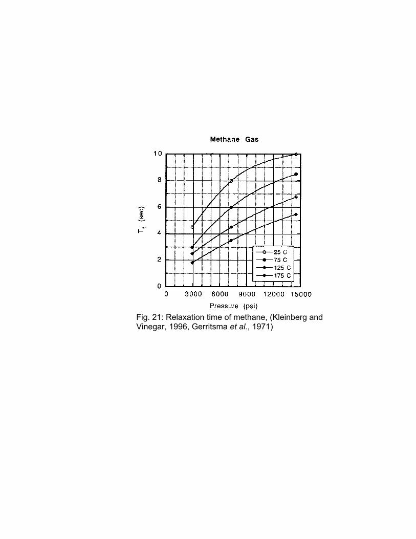
Fig. 21: Relaxation time of methane, (Kleinberg and Vinegar, 1996, Gerritsma et al., 1971)

Methane Self-Diffusion Coefficient, n=0.7

1.4E-06

1.6E-06

1.8E-06

2.0E-06

2.2E-06

2.4E-06

2.6E-06

2.8E-06

3.0E-06

0.0 0.1 0.2 0.3 0.4density (g/cm3)

ρD/T

n (g

/(cm

*s*K

n ))

Harris(298) Haris(323) Dawson(353) Dawson(322)Dawson(297) Oosting(297) Oosting(273) Greiner(295)Greiner(327) Greiner(333) Greiner(364) Greiner(394)Greiner(403) Greiner(427) Greiner(454) Correlation

Fig. 21: Correlation for methane diffusion coefficient

Fig. 23: Methane diffusion coefficient (Kleinberg and Vinegar, 1996)

1.E-02

]Lo]es[Sho-Wei Lo]o]

1.E-06

1.E-05

1.E-04

1.E-03

1.E-02

1.E-05 1.E-04 1.E-03 1.E-02 1.E-01Viscosity/Temperature (cP/K)

D (c

m2 /s

ec)

pure C6[Sho-Wei Lo] pure C10[Sho-Wei Lo]pure C16[Sho-Wei Lo] pure C1[Sho-Wei Lo]linear fit[Sho-Wei Lo] pure C2[ Helbak et al]pure C2[this work] pure C1[Helbak et al]pure C6[Helbak et al]

D=5.05x10-8(T/Visc)

Fig. 24: Diffusion coefficient dependence for alkanes on viscosity/temperature (Y. Zhang, 2001).

1

10

100

1.E-06 1.E-05 1.E-04 1.E-03

Diffusion coefficient (cm2/sec)

T1 (s

ec)

Pure C6[Sho-Wei Lo] Pure C10[Sho-Wei LoPure C16[Sho-Wei Lo] C1+C16 liq[Sho-Wei C1+C16 liquid[Sho-Wei Lo] linear fit for pure alkanC1-C10 liq[Sho-Wei Lo] C1-C6 vap[Sho-Wei LC1-C10 vap[Sho-Wei Lo] Pure C2[this work]

Fig. 25 : T1 dependence on diffusion coefficient (Y. Zhang, 2001).

Fig. 27: Diffusivities of a 825 SCF/STB GOR live oil as function of pressure. The measurements were taken at two different temperatures and are compared to the diffusivity of the same oil after the solution gas has been depleted.

Fig. 26: Distribution of self-diffusion coefficients of a 33º API live crude oil with 825 SCF/STB GOR as function of pressure. The PFG NMR measurements have been made at 75ºF.

Fig. 28: Diffusivities of various live and dead oils and oil-based mud filtrates as function of fluid viscosities over temperature.

0

1

1.E-01 1.E+00 1.E+01T2 (sec)

puresqualene pure

hexane

H(C6)=0.38A(C6)=0.39

H(C6)=0.50A(C6)=0.51

0

1

1.E-01 1.E+00 1.E+01

T2 (sec)

puresqualene

pure hexane

H(C6)=0.69A(C6)=0.73

0

1

2

3

1.E-01 1.E+00 1.E+01T2 (sec)

puresqualene

Fig. 29: Relaxation time distributions of n-hexane and squalene mixtures. Thin line is estimate from bi-exponential fit. (Freedman et al., 2001)

0

2

4

6

8

10

1.E-06 1.E-05 1.E-04

Diffusivity (cm2/s)

puresqualene

pure hexane

H(C6)=0.38A(C6)=0.35

H(C6)=0.50A(C6)=0.52

012345678

1.E-06 1.E-05 1.E-04Diffusivity (cm2/s)

puresqualene

pure hexane

H(C6)=0.69A(C6)=0.61

02468

10121416

1.E-06 1.E-05 1.E-04Diffusivity (cm2/s)

puresqualene

pure hexane

Fig. 30: Diffusivity of n-hexane and squalene mixtures. (Freedman et al., 2001)

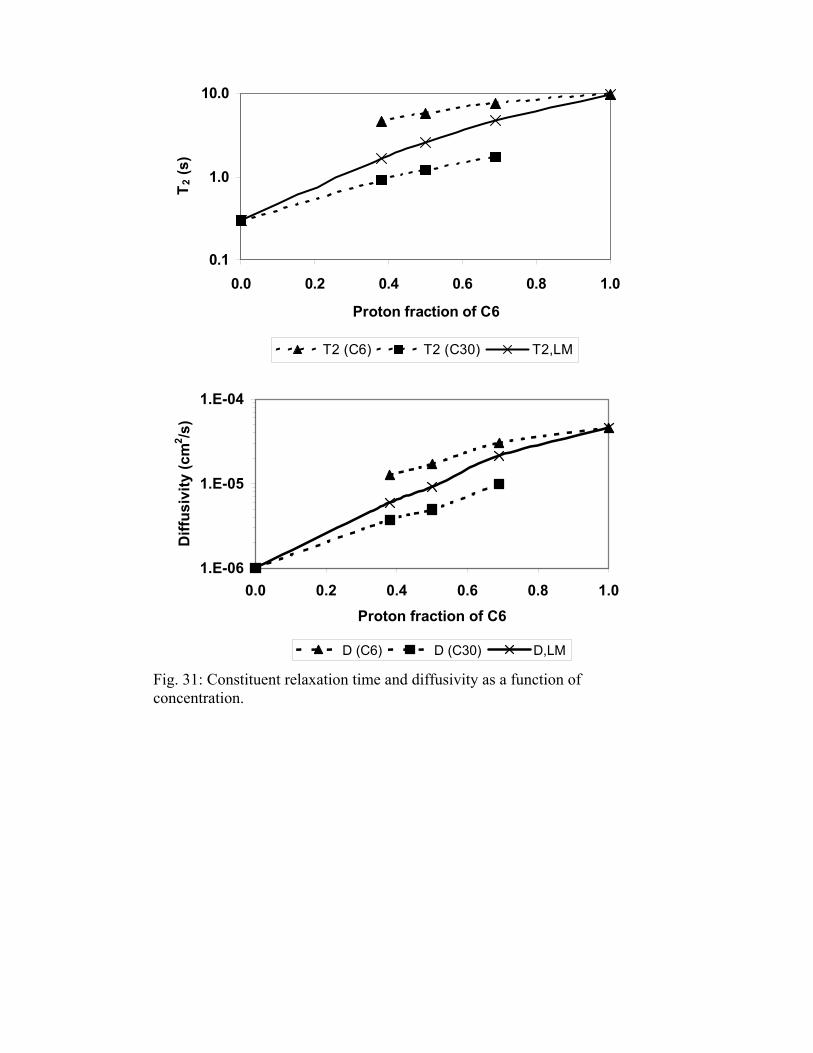
0.1

1.0

10.0

0.0 0.2 0.4 0.6 0.8 1.0

Proton fraction of C6

T 2 (s

)

T2 (C6) T2 (C30) T2,LM

1.E-06

1.E-05

1.E-04

0.0 0.2 0.4 0.6 0.8 1.0Proton fraction of C6

Diff

usiv

ity (c

m2 /s

)

D (C6) D (C30) D,LM

Fig. 31: Constituent relaxation time and diffusivity as a function of concentration.

1.E-06

1.E-05

0.0 0.2 0.4 0.6 0.8 1.0Proton fraction of C6

D/T

2 (cm

2 /s2 )

D/T2(C30) D/T2(C6) b/a

Fig. 32: Ratio of constituent diffusivity and relaxation time compared to that of the correlation.

1.E-07

1.E-06

1.E-05

1.E-04

0.1 1.0 10.0

T2 (sec)

D (c

m2 /s

ec)

D (C6) D (C30) Correlation

pure C30

pure C6

Fig. 33: Correlation between constitutent diffusivity and relaxation time of n-hexane and squalene. The line is the correlation predicted by the constitutive viscosity model (Freedman et al., 2001).

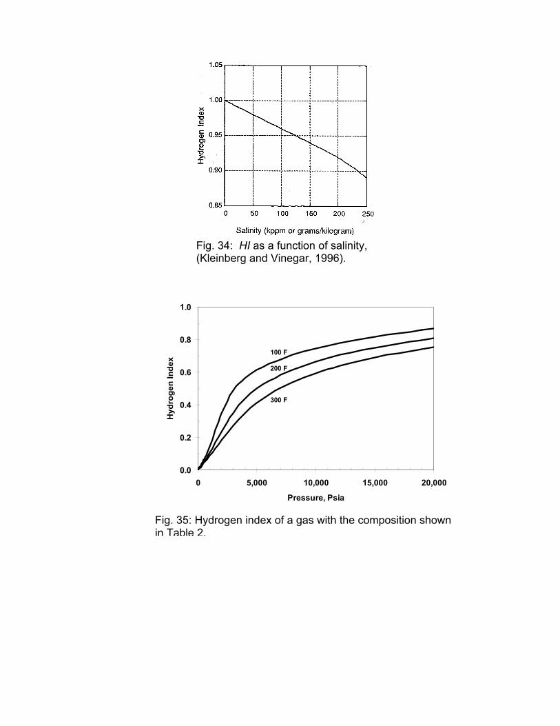
Fig. 34: HI as a function of salinity, (Kleinberg and Vinegar, 1996).

0.0

0.2

0.4

0.6

0.8

1.0

0 5,000 10,000 15,000 20,000

Pressure, Psia

Hyd

roge

n In

dex

100 F

300 F

200 F

Fig. 35: Hydrogen index of a gas with the composition shown in Table 2.

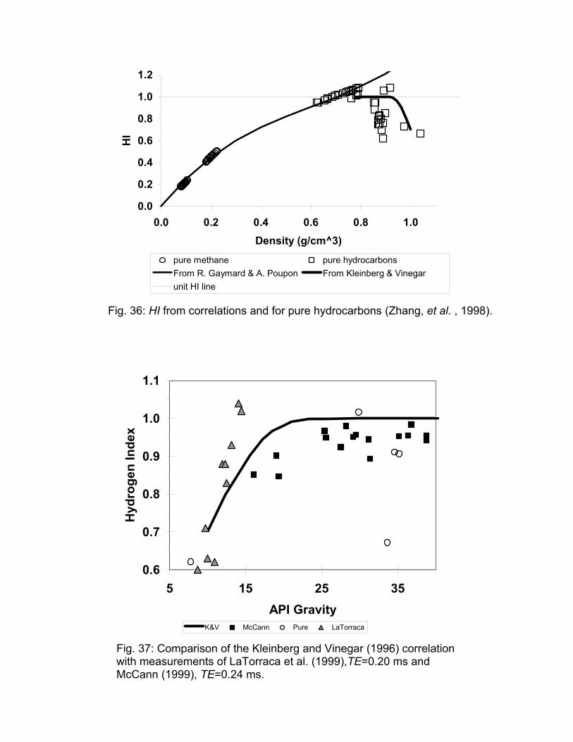
0.0

0.2

0.4

0.6

0.8

1.0

1.2

0.0 0.2 0.4 0.6 0.8 1.0Density (g/cm^3)

HI

pure methane pure hydrocarbonsFrom R. Gaymard & A. Poupon From Kleinberg & Vinegarunit HI line

Fig. 36: HI from correlations and for pure hydrocarbons (Zhang, et al. , 1998).

0.6

0.7

0.8

0.9

1.0

1.1

5 15 25 35API Gravity

Hyd

roge

n In

dex

K&V McCann Pure LaTorraca

Fig. 37: Comparison of the Kleinberg and Vinegar (1996) correlation with measurements of LaTorraca et al. (1999),TE=0.20 ms and McCann (1999), TE=0.24 ms.

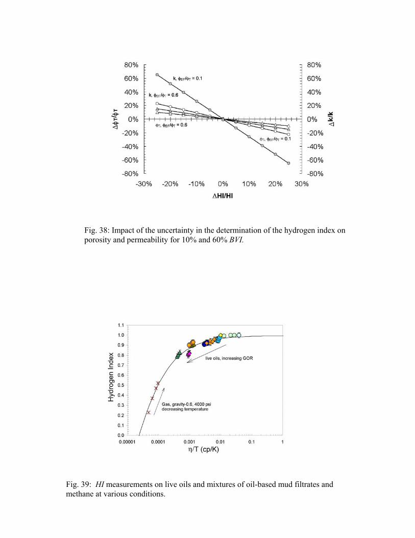
Fig. 38: Impact of the uncertainty in the determination of the hydrogen index on porosity and permeability for 10% and 60% BVI.

Fig. 39: HI measurements on live oils and mixtures of oil-based mud filtrates and methane at various conditions.

0.0

0.2

0.4

0.6

0.8

1.0

1.2

0.0 0.2 0.4 0.6 0.8 1.0

Density (g/cm3)

HI

1.2

SM (STO)SM (live oil)SMY (STO)SMY (live oil)G&PK&V

H:C=4:1 3:1 2:1

1:1

Fig. 40: Calculated HI for two live crude oils (Q. Zhang, 2001).