NKS-341 ISBN 978-87-7893-423-9

Software reliability analysis for PSA:

failure mode and data analysis

Ola Bäckström1

Jan-Erik Holmberg2

Mariana Jockenhövel-Barttfeld3

Markus Porthin4

Andre Taurines3

Tero Tyrväinen4

1Lloyds Register AB, Sweden 2Risk Pilot AB, Sweden

3AREVA GmbH, Germany 4VTT Technical Research Centre of Finland Ltd

July 2015

Abstract This report proposes a method for quantification of software reliability for the purpose probabilistic safety assessment (PSA) for nuclear power plants. It includes a failure modes taxonomy outlining the relevant software failures to be modelled in PSA, quantification models for each failure type as well as an analysis of operating data on software failures concerning the TELEPERM® XS (TXS) platform developed at AREVA.

Software related failure modes are defined by a) their location, i.e., in which module the fault is, and b) their effect on the I&C unit. For a proces-sor the effect is either a fatal failure of the processor (termination of the function and no outputs are produced) or non-fatal failure where operation continues with possible wrong output values. Following cases are relevant from the PSA modelling point of view: 1) fatal failure causing loss of all subsystems that have the same system software, 2a) fatal failure causing loss of one subsystem, due to fault in system software, 2b) fatal failure in communication modules of one subsystem. 3) fatal failure causing failure of redundant set of I&C units in one subsystem, 4) non-fatal failure associ-ated with an application software module. In the case 4, the failure effect can be a failure to actuate the function or a spurious actuation.

The failure rates for software fault cases 1 and 2, associated with the sys-tem software, are proposed to be estimated from general operational data for same system software. The probabilities on failure on demand for cases 3 and 4, associated with the application software, are a priori as-sumed to correlate with the complexity and degree of verification and vali-dation (V&V) of the application. The degree of V&V is related to the safety class of the software system and the complexity can be assessed by ana-lysing the logic diagram specification of the application. A priori estimates could be updated by operational data, which is demonstrated in the report. Key words PSA, Software reliability, Failure mode, Operational history data NKS-341 ISBN 978-87-7893-423-9 Electronic report, July 2015 NKS Secretariat P.O. Box 49 DK - 4000 Roskilde, Denmark Phone +45 4677 4041 www.nks.org e-mail nks@nks.org

1

Software reliability in PSA: failure mode and data analysis

Report from the NKS-R DIGREL activity (Contract: AFT/NKS-R(14)86/3)

Ola Bäckström1

Jan-Erik Holmberg2

Mariana Jockenhövel-Barttfeld3

Markus Porthin4

Andre Taurines3

Tero Tyrväinen4

1Lloyds Register AB, P.O. Box 1288, SE-172 25 Sundbyberg, Sweden

2Risk Pilot, Parmmätargatan 7, SE-11224 Stockholm, Sweden

3AREVA GmbH, P.O. Box 1109, 91001 Erlangen, Germany

4VTT Technical Research Centre of Finland Ltd, P.O. Box 1000, FI-02044 VTT, Finland

2

Table of contents

Table of contents 2

Abbreviations 5

Summary 6

Acknowledgements 7

1. Introduction 8

2. Literature review 9

2.1 Software reliability quantification 9

2.2 Software reliability estimation in PSA 10

2.2.1 Screening out approach 11

2.2.2 Screening value approach 11

2.2.3 Expert judgement approach 11

2.2.4 Operating experience approach 12

2.3 Conclusions on software reliability in PSA 12

3. Definitions and concepts 13

4. Overview of the software fault mode analysis and quantification method 17

4.1 Software fault cases 17

4.2 Outline of the quantification method 19

4.3 System software (SyS) 20

4.4 Application software 20

4.4.1 Application software, functions and modules 20

4.4.2 Estimation of the application software module failure probability 25

4.4.3 Classification of application software faults, failures and failure effects 28

5. Analysis of operating experience 30

5.1 Assessment of system software failures 31

5.1.1 TXS operating experience 31

3

5.1.2 Reliability assessment of SyS software 31

5.2 Assessment of application software failures 33

5.2.1 Applicability of the TXS operating experience 35

5.3 Estimation of application software failures using TXS operating experience 36

5.3.1 Estimation of failure fractions 36

5.3.2 Assessment of self-announcing application software failures 38

5.3.3 Assessment of not-self-announcing application software failures 40

5.3.4 Assessment of the application software failure modes 43

5.3.5 Estimation of failures for application software modules 44

6. Reliability assessment of application software modules 47

6.1 Evidence on the reliability of application software modules 47

6.2 V&V level 47

6.3 Complexity 48

6.3.1 General discussion 48

6.3.2 Factors that affect complexity 48

6.3.3 Methods to assess complexity 49

6.3.4 ISTec 50

6.3.5 SICA 51

6.3.6 Extended complexity vector 51

6.3.7 Examples 51

6.3.8 Assessment of complexity degree of a logical diagram 53

6.4 Estimation of probabilities of AS modules 54

6.4.1 Failure announcing based estimate; SA and non-SA estimation 55

6.4.2 Failure mode based estimate; fatal and non-fatal failures 58

6.4.3 Examples 60

6.5 CCF between related AS modules 62

7. Summary of failure data evaluation process 63

4

8. Case study with the example PSA model 65

9. Conclusions 66

10. References 69

Appendix A. Software complexity analysis 73

Appendix B. Justification of failure fractions of application software failures 78

Appendix C. Estimation of number of demands to the TXS-based I&C systems 82

Appendix D. Example PSA model 84

5

Abbreviations

A&P Acquisition and processing

AF Application function

APU Acquisition and processing unit

AS Application software (module)

BBN Bayesian Belief Net

BWR Boiling water reactor

CCF Common cause failure

CDF Core damage frequency

DCU Data communication unit

DCS Data communication software

DIGREL

DLC

Reliability analysis of digital systems in PSA context. Research project

financed by NKS, SAFIR2014 and Nordic PSA Group

Data link configuration

DPS Diverse protection system

EF Elementary function

EFW Emergency feedwater system

FRS Functional requirement specification

HW Hardware

I&C Instrumentation and control

IEC International Electrotechnical Commission

MSI Monitoring and service interface

NKS Nordic nuclear safety research

NPP Nuclear power plant

NPSAG Nordic PSA Group

OECD/NEA Organisation for Economic Co-operation and Development, Nuclear

Energy Agency

PACS Priority actuator control system

pfd Probability of failure on demand

PSA Probabilistic safety assessment

RCS Reactor control

RLS Reactor limitation system

RPS Reactor protection system

RTE Run time environment

SA Self-announcing

SAFIR Finnish Research Programme on Nuclear Power Plant Safety

SCDS Signal condition and distribution system

SIL Safety Integrity Level (as defined in IEC 61508)

SIVAT Simulation-based validation tool of TXS

SPACE Specification and coding environment of TXS

SS Subsystem

SyS System software

SW Software

TXS TELEPERM® XS, product of AREVA

V&V Verification and validation

VTT Technical Research Centre of Finland Ltd

VU Voting unit

6

Summary

The advent of digital I&C systems in nuclear power plants has created new challenges for

safety analysis. To assess the risk of nuclear power plant operation and determine the risk

impact of digital systems, there is a need to quantitatively assess the reliability of the digital

systems in a justifiable manner. Due to the many unique attributes of digital systems, a

number of modelling and data collection challenges exist, and consensus has not yet been

reached. It is however agreed that software failures are relevant and should be considered

probabilistically in PSA.

This report proposes a method for quantification of software reliability for the purpose PSA

for nuclear power plants, developed in the Nordic DIGREL project. It includes a failure

modes taxonomy outlining the relevant software failures to be modelled in PSA,

quantification models for each failure type as well as an analysis of operating data on software

failures concerning the TELEPERM® XS (TXS) platform developed at AREVA.

Software related failure modes can be defined by a) their location, i.e., in which module the

fault is, and b) their effect on the I&C unit. For a processor the effect is either a fatal failure of

the processor (termination of the function and no outputs are produced) or non-fatal failure

where operation continues with possible wrong output values. Following cases are relevant

from the PSA modelling point of view:

1. Fatal failure causing loss of all subsystems that have the same system software and

similar application software. The processors of both subsystems stop the cyclic

processing and output signals are set to “fail-safe” values.

2. Fatal failure causing loss of one subsystem

a. Fault is in system software. The whole subsystem stops running and outputs are

set to 0.

b. Fatal failure in communication modules of one subsystem. The voting units run

and take default values.

3. Fatal failure causing failure of redundant set of I&C units, i.e. a set of acquisition and

processing units or a set of voting units in one subsystem. This failure can be caused

by an application software fault.

4. Non-fatal failure associated with an application software module. Failure effect can be

a failure to actuate the function or a spurious actuation. The fault can be in the

acquisition and processing units or voting units.

The failure rates for software fault cases 1 and 2, associated with system software, are

proposed to be estimated from operational data. However, only a few failures belonging to

case 2b are found in the analysed TXS data. The failure probabilities for cases 3 and 4,

associated with application software failures, are assumed to correlate with the complexity

and degree of verification and validation (V&V) of the software. The degree of V&V is

related to the safety class of the software system and the complexity can be assessed by

analysing the logic diagram specification of the application software module. In principle, the

a priori estimates could be updated by operational data. Although very few demands for the

reactor protection system during operation are reported, considerably more demands are found

for other safety related I&C systems implemented by the same platform. This opens an

opportunity to use operational data. Such data has been analysed by AREVA using Bayesian

estimation, which is demonstrated in the report.

7

Acknowledgements

The work has been financed by NKS (Nordic nuclear safety research), SAFIR2014 (The

Finnish Research Programme on Nuclear Power Plant Safety 2011–2014) and the members of

the Nordic PSA Group: Forsmark, Oskarshamn Kraftgrupp, Ringhals AB and Swedish

Radiation Safety Authority. NKS conveys its gratitude to all organizations and persons who

by means of financial support or contributions in kind have made the work presented in this

report possible.

The AREVA authors are very thankful to Dr. Christian Hessler for the interesting discussions

and for his support to this work.

Disclaimer

The views expressed in this document remain the responsibility of the author(s) and do not

necessarily reflect those of NKS. In particular, neither NKS nor any other organization or

body supporting NKS activities can be held responsible for the material presented in this

report.

8

1. Introduction

Digital instrumentation and control (I&C) systems are appearing as upgrades in older nuclear

power plants (NPPs) and are commonplace in new NPPs. To assess the risk of NPP operation

and to determine the risk impact of digital system upgrades on NPPs, quantifiable reliability

models are needed along with data for digital systems that are compatible with existing

probabilistic safety assessments (PSAs). Due to the many unique attributes of these systems

(e.g., complex dependencies, software), several challenges exist in systems analysis,

modelling and in data collection

Currently there is no consensus on reliability analysis approaches for digital I&C. Traditional

event and fault tree methods have limitations, but more dynamic approaches are still in trial

stage and are difficult to apply in full scale PSA-models. Distributed control systems are

typically analysed and modelled rather simply. Digital control systems can furthermore be

analysed on several abstraction levels, which raises additional questions, such as: which level

of detail should be used, which failure modes should be considered, how to consider software

(SW) failures, which dependencies should be considered, how to account for human errors

etc. Selection of plausible failure data, including common cause failure data for hardware and

software failures is an open issue. An important issue is also the objective of the analysis: Is it

an analysis of the digital system itself, or is it an analysis of the digital system in a context

where only some of the failures are critical?

This report presents the work on software reliability quantification of the Nordic DIGREL

project (Reliability analysis of digital systems in PSA context) financed by NKS, SAFIR2014

and Nordic PSA Group. The current report complements the main report of the project,

presented in (Authén et al. 2015). The activities in the project are closely related to on an

activity performed by the OECD/NEA Working Group RISK and to the Euratom FP7 project

HARMONICS (http://harmonics.vtt.fi/).

The overall objectives of the project are to provide guidelines to analyse and model digital

systems in PSA context, using traditional reliability analysis methods (failure mode and

effects analysis, fault tree analysis). Based on the pre-study questionnaire and discussions with

the end users in Finland, Sweden and within the WGRISK community, the following focus

areas have been identified for the activities:

1. Develop a taxonomy of hardware and software failure modes of digital components for

common use. (Authén et al. 2015)

2. Develop guidelines for failure modes analysis and fault tree modelling of digital I&C.

(Authén et al. 2015)

3. Develop an approach for modelling and quantification of software (this report).

The current report aims at developing a method for quantification of software reliability to be

used in PSA for nuclear.

9

2. Literature review

This chapter gives an overview of the state-of-the-practice in software reliability analysis in

PSA. Software failures are in general mainly caused by systematic (i.e. design specification or

modification) faults, and not by random errors. Software based systems cannot easily be

decomposed into components, and the interdependence of the components cannot easily be

identified and modelled. Modelling software reliability in the PSA context is hence not a

trivial matter.

Software reliability models usually rely on assumptions and statistical data collected from

non-nuclear domains and therefore may not be directly applicable for software products

implemented in NPPs. More important than the exact values of failure probabilities are the

proper descriptions of the impact that software-based systems has on the dependence between

the safety functions and the structure of accident sequences. The conventional fault tree

approach is, however, considered sufficient for the modelling of the reactor protection system

(RPS) like functions.

In spite of the unsolved issue of addressing software failures there seems be a consensus

regarding philosophical aspects of software failures and their use in developing a probabilistic

model. The basic question: “What is the probability that a safety system or a function fails

when demanded” is a fully feasible and well-formed question for all components or systems

independently of the technology on which the systems are based (Dahll et al. 2007). A similar

conclusion was made in the Workshop on Philosophical Basis for Incorporating Software

Failures in a Probabilistic Risk Assessment (Chu et al. 2010). As part of the open discussion,

the panelists unanimously agreed that:

• software fails

• the occurrence of software failures can be treated probabilistically

• it is meaningful to use software failure rates and probabilities

• software failure rates and probabilities can be included in reliability models of digital

systems.

2.1 Software reliability quantification

For the quantification of software failure rates and probabilities there are several general

approaches, e.g., reliability growth methods, Bayesian belief network (BBN) methods, test

based methods, rule based methods (Dahll et al. 2007) and software metrics based methods

(Smidts & Li 2000, 2004). These methods are reviewed by Chu et al. 2010. None of the

methods for quantifying digital systems reliability is universally accepted, in particular for

highly reliable systems (EPRI 2010).

Software reliability models can be divided into white box models, which consider the

structure of the software in estimating reliability, and black box models, which only consider

failure data, or metrics that are gathered if test data is not available (Zhang 2004). Black box

models generally assume that faults are perfectly fixed upon observation without introducing

any new faults. Software reliability is thus increasing over time. Such models are known as

Software Reliability Growth Models (SRGMs). Reliability growth models are based on the

sequence of times between observed and repaired failures (Dahll et al. 2007). The models

calculate the reliability and the current failure rate. Additionally, the reliability growth models

can predict the time to next failure and required time to remove all faults.

10

Many of these have predictive power only over the short term, but long term models have also

been developed (Bishop & Bloomfield 1996).

The BBN methodology has been adapted to software safety assessment (Haapanen et al. 2004)

and the methodology can be considered as promising. One of the main drawbacks is that a

different BBN has to be built for each software development environment. This problem may

be solved by using generalized BBN templates which are not restricted to a specific

development environment (Eom et al. 2009). Application of BBN is further discussed in

Section 4.

In test based methods a program is executed with selected data and the answer is checked

against an ‘oracle’. A reliability measure can be generated, by running a number of tests and

measuring the number of failures. Test-based reliability models assume that the input data

profile used during the test corresponds to the input profile during real operation.

Unfortunately, this correspondence cannot often be guaranteed. Statistical testing may be,

however, used as an input to a BBN model.

Context-based Software Risk Model (CSRM) allows assessing the contribution of software

and software-intensive digital systems to overall system risk in a way that can be integrated

with the PSA format used by NASA (Yau & Guarro 2010, Guarro 2007, Vesely et al. 2002).

A combination of operating experience and engineering judgment can be used to provide

estimates for digital system software common-cause failures (CCF) (Enzinna et al. 2009).

2.2 Software reliability estimation in PSA

In the context of PSA for NPPs, there is an on-going discussion on how to treat software

reliability in the quantification of reliability of systems important to safety. It is mostly agreed

that software could and should be treated probabilistically (Dahll et al. 2007, Chu et al. 2009)

but the question is to agree on a feasible approach.

Software reliability estimation methods described in academic literature, shortly discussed in

the previous chapter, are not applied in real industrial PSAs for NPPs. Software failures are

either omitted in PSA or modelled in a very simple way as common cause failures (CCF)

related to the application software (AS) of operating system (platform). It is difficult to find

any basis for the numbers used except the reference to a standard statement that 1E-4 per

demand is a lower limit to reliability claims, which limit is then categorically used as a

screening value for software CCF.

The engineering judgement approaches used in PSA can be divided into the following

categories depending on the argumentation and evidence they use (Bäckström & Holmberg

2012):

• screening out approach

• screening value approach

• expert judgement approach

• operating experience approach.

The reliability model used for software failures is practically always the simple “probability of

failure per demand” (pfd).

11

2.2.1 Screening out approach

Screening out approach means that software failures are screened out from the model. The

main arguments to omit software are that 1) the contribution of software failures is

insignificant or that 2) no practical method to assess the probability of software failure

(systematic failure) exists.

One approach is to model software failures but not to define reliability values. The impact of

software failures is assessed through sensitivity approaches. This approach has been utilized,

for instance, in Ringhals 2 (Authén et al. 2010). In another approach, values 0, 1E-4 and 1E-3

for pfd were used in sensitivity analyses as software failure probabilities to analyse the impact

of software failures on the system unavailability and the plant risk (Kang & Jang 2009).

2.2.2 Screening value approach

Screening value approach means that some reliability number, like pfd = 1E-4, is chosen

without detailed assessment of the reliability, and it is claimed that this is a conservative

number for a software CCF. The screening value is taken from a reference like IEC 61226

(IEC 2005). Accordingly, the “Common Position” document states that reliability claims “q <

1E-4” for a single software based system important to safety shall be treated with extreme

caution (SSM 2010). This derives partly due to the fact that demonstrating lower probabilities,

e.g. by statistical testing is very laborious.

2.2.3 Expert judgement approach

The expert judgement approach relies on the assessment of the features of the software system

which are assumed to have correlation with the reliability. The two questions are 1) which

features should be considered and 2) what is the correlation between the features and the

reliability. This kind of approach is used extensively in PSA, e.g., in human reliability

analysis. Such models are difficult to validate.

In a case study on quantitative reliability estimation of a software-based motor protection

relay, Bayesian networks were used to combine evidence from expert judgment and

operational experience (Haapanen et al. 2004).

In one study, it was assumed that the contribution from software failure to total failure

probability is 10% of the hardware failure probabilities (Varde et al. 2003). The rationale to

this was that there are two well recognized aspects of software reliability: 1) the contribution

of software failures to total failure of a digital system is smaller compared to exclusive failure

of hardware, 2) there is a threat of software related common cause failures for a group of

identical and redundant components. The second aspect was addressed by selecting a suitable

value for β in the beta-factor CCF model. Value β = 0.03 was given, including CCFs due to

hardware and software.

The safety integrity level value approach (SIL; IEC 61508) (IEC 2010) is also an example of

an expert judgement approach, where the reliability target implied by the SIL is interpreted as

the unavailability of the item. To apply SIL-values is a controversial issue, and at least the

following weaknesses may be mentioned (EPRI 2010): it does not differentiate between

functions implemented by the system and the failure modes of the system; it is silent regarding

the contribution of systematic failures; it does not give any indication for the estimation of

12

beta-factors or other parameters that can be used to characterize CCFs; the notion of “system”

is not defined.

2.2.4 Operating experience approach

The operating experience approach means an assessment based on operational data. In reality,

the operating experience approach is like the expert judgement approach since operational

data need to be interpreted in some way to be used for reliability estimation.

In the PSA study of the Swedish NPP Ringhals 1, the contribution of software CCF to the

unavailability of a safety system was assessed based on operational experience (Authén et al.

2010b). The operational experience of over 60 similar systems showed no CCF caused by

platform properties and thus the contribution of platform CCF was estimated at 1E-8 (pfd).

Two events could be considered as a CCF, which leads to an unavailability of safety I&C

systems as 1E-6 (pfd). This pfd value was applied for redundant I&C units.

In one study (Enzinna et al. 2009), reasonable estimates for the relative contribution of

software to digital system reliability software CCF probabilities were developed based on

operational experience and engineering judgment. The CCF probability of operating system

software was estimated as 1E-7 based on data gathered from dozens of plants during a time

period of more than 10 years. For the application software, the CCF probability was estimated

as 1E-5 for each function group. The SIL-4 targets were used as a general guide in the

estimate. Additionally, it is suggested that if multiple application software CCFs appeared in

same cut set the dependency between the two CCFs should be assessed. One way to take this

into consideration is to assume a beta factor between the two software CCF events. Values

0.001 < β < 0.1 were recommended, depending on the similarity of the software.

2.3 Conclusions on software reliability in PSA

Generally, only common cause failures are modelled in PSA. One reason for this is that there

has not been a methodology available to correctly describe and incorporate software failures

into a fault tree model. The only reliability model which is applied is constant unavailability

and this is used to represent the probability of CCF per demand. Spurious actuations due to

software failures are not modelled or it has been concluded that there is no need to consider

software failure caused spurious actuations.

Software CCF is usually understood as the application software CCF or its meaning has not

been specified. Software CCF is generally modelled between processors performing redundant

functions, having the same application software and on the same platform. One of the

exceptions is the design phase PSA made for the automation renewal of the Loviisa NPP,

where four different levels of software failures are considered: 1) single failure, 2) CCF of a

single automation system, 3) CCF of programmed systems with same platforms and/or

software, and 4) CCF of programmed systems with different platforms and/or software

(Jänkälä 2011).

It is difficult to trace back where the reliability numbers used in PSA come from — even in

the case of using operating experience. The references indicate the sort of engineering

judgement but lacks supporting argumentation.

13

3. Definitions and concepts

Active failure: An active failure leads to a spurious actuation of a function.

Application function: function of an I&C system that performs a task related to the process

being controlled rather than to the functioning of the system itself. Also referred to as I&C

function.

Application software (module): piece of software that is represented by a specific group of

lines of source code (or equivalent graphical representation, e.g. function diagrams) and has a

specific functionality. The application software is the representation of the application

functions in form of code. The application software is executed and controlled by the system

software (run time environment) during an operating cycle.

There are usually several AS modules associated with each I&C function but not all AS

modules are necessarily relevant for the safety function considered in PSA. Based on

(AREVA 2013) the following software modules can be defined as relevant to describe one

application in the PSA:

A&P-AS: Application software module for acquisition and processing (A&P) of input

signals. This module includes the software for preprocessing/reading the input

signals in the acquisition and processing unit (APU) to perform the signal

conversion, plausibility checks1, evaluation of the signal status.

APU-AS: Application software module for the implementation of the specific functionality

in the processor of the APU. The results of the signal processing are distributed

to the actuation (voter) computers.

VU-AS: Application software module for the actuation implemented in the processor of

the voter unit (VU).

Each software module usually corresponds to one individual function diagram group

dedicated to a specific task. Depending on the specific case the application software can be

represented by one or more AS modules.

Data communication software (DCS): This software module implements the data

communication protocol. It is part of the platform software.

Data link configuration (DLC): This software module is provided in the form of a data table.

It specifies the nodes that can be part of a given network, and the data messages that can be

exchanged between the nodes of the network.

Demand: A plant state or an event that requires an action from I&C. A demand to an I&C

system occurs when a signal value exceeds or falls below a certain threshold. The command is

1 Range checks for analogue signals, non-coincidence checks for binary signals.

14

activated with a request. Note: A state of the I&C system requiring an action of an active fault

tolerant design feature is not considered a demand.

In this report, “demand” is used in the same meaning as in the reliability metric “probability

per demand”, and is a specific uncovering situation, which is distinct from dedicated failure

detection mechanisms such as online and offline monitoring. Online and offline monitoring

are means to detect a failure before a demand.

Detected failure: A failure detected by (quasi-) continuous means, e.g. online detection

mechanisms, or by plant behaviour through indications or alarms in the control room.

Detection mechanism: The means or methods by which a failure can be discovered by an

operator under normal system operation or can be discovered by the maintenance crew by

some diagnostic action (US DOD 1984). Note that this includes detection by the system (e.g.

continuous detection).

There are two categories of detection mechanisms:

Online detection mechanisms. Covers various continuous detection mechanisms.

Offline detection mechanisms. E.g. periodic testing and also other kind of controls

(e.g. maintenance).

Fail safe: Pertaining to a functional unit that automatically places itself in a safe operating

mode in the event of a failure (ISO/IEC/IEEE 2010); “system or component” has been

replaced with “functional unit”) Example: a traffic light that reverts to blinking yellow in all

directions when normal operation fails. Note: In general, fail safe functional units do not show

fail safe behaviour under all possible conditions.

Failure: Termination of the ability of a product to perform a required function or its inability

to perform within previously specified limits (ISO/IEC 2005). "Failure" is an event, as

distinguished from "fault" which is a state.

Failure effect: Consequence of a failure mode in terms of the operation, function or status

(IEC 2006, “of the system” removed).

Failure mode: The physical or functional manifestation of a failure (ISO/IEC/IEEE 2010).

Failure mechanism: Relation of a failure to its causes.

Fatal failure: failures that cannot be handled specifically, as their source and effect are not

known completely during cyclic processing. Only termination of system operation is suitable

to avoid unintended system response. The I&C unit or the hardware module stalls. It ceases

functioning and does not provide any exterior sign of activity. Fatal failures may be

subdivided into:

Ordered fatal failure: The outputs of the I&C unit or the hardware module are set to

specified, supposedly safe values. The means to force these values are usually exclusively

hardware. Equivalent to the definition “Halt/abnormal termination of function with clear

message” (Chu et al. 2006).

15

Haphazard fatal failure: The outputs of the I&C unit or the hardware module are in

unpredictable states. Equivalent to the definition “Halt/abnormal termination of function

without clear message” (Chu et al. 2006).

Fault: Defect or abnormal condition that may cause a reduction in, or loss of, the capability of

a functional unit to perform a required function (IEC 2010a; “defect” added). Note: "Failure"

is an event, as distinguished from "fault" which is a state.

Fault tolerance: The ability of a functional unit to continue normal operation despite the

presence of failures of one or more of its subunits. Note: Despite the name this definition

refers to failures, not faults of subunits. It is therefore distinct from the definition in

(ISO/IEC/IEEE 2010). Possible means to achieve fault tolerance include redundancy,

diversity, separation and fault detection, isolation and recovery.

Function block: reusable, closed, and classifiable piece of software, capable of processing

signals, from which I&C functions can be assembled using function diagrams. Function

blocks operate in a closed and well-defined manner. Also called elementary function.

Function diagram: diagram that specifies the application software to be run within an I&C

system by connecting function blocks with each other and with external signals.

Functional requirements specification (FRS): documentation that describes the requested

behaviour of an engineering system and includes the operation and activities that a system

must be able to perform.

Global effect (AS faults with): Faults that affect several applications running on the

processor. In the worst case all applications allocated on the processor are affected, e.g.

shutdown of the processor via an exception handler.

Initiating event: An initiating event is an event that could lead directly to core damage (e.g.

reactor vessel rupture) or that challenges normal operation and which requires successful

mitigation using safety or non-safety systems to prevent core damage (IAEA 2010).

Local effect (AS faults with): Faults that affect only the faulty application and the processor

continues the cyclic processing (all other applications are unaffected).

Non-fatal failure: for non-fatal errors a suitable processing is applied to limit the failure

effect and continue cyclic processing of not affected functions. The affected I&C unit or the

hardware module fails but it continues to generate outputs. Non-fatal failures may be

subdivided into:

Failures with plausible behaviour: I&C runs with wrong results that are not evident

(Chu et al. 2006). An external observer cannot determine whether the I&C unit or the

hardware module has failed or not. The unit is still in a state that is compliant to its

specifications, or compliant to the context perceived by the observer.

Failures with implausible behaviour: I&C runs with evidently wrong results (Chu et al.

2006). An external observer can decide that the I&C unit or the hardware module has

failed. The unit is clearly in a state that is not compliant to its specifications, or not

compliant to the context perceived by the observer.

16

Not-self-announcing fault: A not-self-announcing AS fault is a fault that cannot be detected

by the I&C system itself. NSA faults with a passive failure can only be revealed by an

observer in case of a demand. NSA faults with active failure could be observed both during

plant operation and at a demand, since these would lead to an unexpected signal.

Passive failure: A passive failure leads to an unavailability of the output signal, i.e. failure to

actuate.

Proprietary software: code that is embedded in specific hardware modules, different from

the microprocessor module of APU, VU and data communication unit (DCU), and that

performs a function of its own. It can be also designated as “software in COTS”. This

software is proprietary and its source code is generally not available for the end user.

Self-announcing fault: A self-announcing AS fault is a fault which is detected by the I&C

system via self-monitoring. The fault is displayed in an interface such that the operator can

exactly find the location of the fault in the I&C system.

Spurious actuation: A failure where an actuation of an I&C function occurred without a

demand. Spurious actuation can be caused by any failure between the process measurement

sensors and the actuator, including erroneous operator command or failure of watchdogs. A

spurious actuation can result in an unintended actuator movement (e.g. start of a pump,

opening of a valve) or in an unintended command termination (e.g. stop of a pump).

System software: The operating system and runtime environment (interaction between

application and operating system).

Systematic failure: Failure related in a deterministic way to a certain cause, which can only

be eliminated by a modification of the design or of the manufacturing process, operational

procedures, documentation or other relevant factors (IEC 2010a).

Undetected failure: A failure detected only by offline detection mechanisms or by demand.

Also called latent failure or hidden failure.

17

4. Overview of the software fault mode analysis and quantification method

For the purpose of defining software fault cases and demonstrating quantification approaches,

a generic safety I&C architecture of an example protection system is assumed. This protection

system consists of two diverse subsystems, called RPS-A and RPS-B, both divided into four

physically separated divisions. The platforms of both subsystems are assumed to be identical.

The extent of diversity between RPS-A and RPS-B may vary, but it is assumed that both

subsystems perform different functions. The number of acquisition and processing units

(APU) and voting units (VU) per each subsystem and division may vary, too, but here we

assume that there can be more than one APU/VU per each subsystem and division.

4.1 Software fault cases

The approach to identify the relevant fault cases is to successively postulate software faults

and triggers for each software module regardless of the likelihood of such faults, and to

determine the maximum possible extent of the failure. The following software modules are

considered (OECD 2014):

System software (SyS).

Elementary functions (EFs)2.

APU functional requirements specification modules (APU-FRS).

APU application software modules (APU-AS).

Proprietary software (Propr. SW) in I&C.

VU functional requirements specification modules (VU-FRS).

VU application software modules (VU-AS).

Data communication software (DCS).

Data link configuration (DLC).

Depending on the location of the software fault, failure effect and system architecture, one or

more units in one or more subsystems can be impacted. The report Failure modes taxonomy

for reliability assessment of digital I&C systems for PRA (OECD 2014) presents a list of

maximum failure extents of a postulated event. Because it would be impractical to take all of

them into consideration in the PSA model, the most relevant can be identified. The software

faults and effects presented in Table 1 are considered further in this report.

2 For TELEPERM

® XS elementary functions are called function blocks. EF can be considered as part of the

system software. However, all the application-specific processing is done in the code of the elementary functions

modules. For this reason, EF could be considered as part of the application software.

18

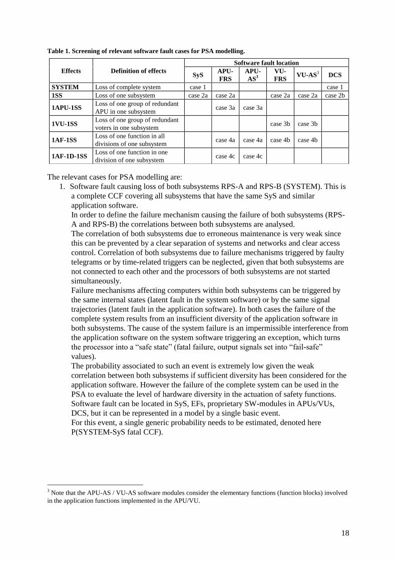
Table 1. Screening of relevant software fault cases for PSA modelling.

The relevant cases for PSA modelling are:

1. Software fault causing loss of both subsystems RPS-A and RPS-B (SYSTEM). This is

a complete CCF covering all subsystems that have the same SyS and similar

application software.

In order to define the failure mechanism causing the failure of both subsystems (RPS-

A and RPS-B) the correlations between both subsystems are analysed.

The correlation of both subsystems due to erroneous maintenance is very weak since

this can be prevented by a clear separation of systems and networks and clear access

control. Correlation of both subsystems due to failure mechanisms triggered by faulty

telegrams or by time-related triggers can be neglected, given that both subsystems are

not connected to each other and the processors of both subsystems are not started

simultaneously.

Failure mechanisms affecting computers within both subsystems can be triggered by

the same internal states (latent fault in the system software) or by the same signal

trajectories (latent fault in the application software). In both cases the failure of the

complete system results from an insufficient diversity of the application software in

both subsystems. The cause of the system failure is an impermissible interference from

the application software on the system software triggering an exception, which turns

the processor into a “safe state” (fatal failure, output signals set into “fail-safe”

values).

The probability associated to such an event is extremely low given the weak

correlation between both subsystems if sufficient diversity has been considered for the

application software. However the failure of the complete system can be used in the

PSA to evaluate the level of hardware diversity in the actuation of safety functions.

Software fault can be located in SyS, EFs, proprietary SW-modules in APUs/VUs,

DCS, but it can be represented in a model by a single basic event.

For this event, a single generic probability needs to be estimated, denoted here

P(SYSTEM-SyS fatal CCF).

3 Note that the APU-AS / VU-AS software modules consider the elementary functions (function blocks) involved

in the application functions implemented in the APU/VU.

Effects Definition of effects

Software fault location

SyS APU-

FRS

APU-

AS3

VU-

FRS VU-AS

3 DCS

SYSTEM Loss of complete system case 1 case 1

1SS Loss of one subsystem case 2a case 2a case 2a case 2a case 2b

1APU-1SS Loss of one group of redundant

APU in one subsystem case 3a case 3a

1VU-1SS Loss of one group of redundant

voters in one subsystem case 3b case 3b

1AF-1SS Loss of one function in all

divisions of one subsystem case 4a case 4a case 4b case 4b

1AF-1D-1SS Loss of one function in one

division of one subsystem case 4c case 4c

19

2. Software fault causing loss of one subsystem (1SS). This is a complete CCF causing a

fatal failure which crashes the processing units in one subsystem, i.e. transition of the

computers to a shut-down state. The software fault can be located in

a) the SyS, EF (APU/VU), APU-FRS, proprietary SW-modules in APUs/VUs, VU-

FRS or VU-AS,

b) DCS or DLC.

The difference is that in case of fatal failure in DCS or DLC (b), VUs run and can take

safe fail states. In case (a), the whole subsystem stops running and also takes a safe

state.

For each case, a generic probability needs to be estimated, denoted here P(1SS-SyS

fatal CCF) resp. P(1SS-DCU fatal CCF).

3. Software fault causing failure of a redundant set of APUs (3a, see Table 1) or VUs (3b)

in one subsystem (1APU, 1VU, respectively). This is a fatal failure causing loss of all

functions. This fault could be due to the same system software subject to identical

states4 or due to the same application software subject to the same set of input data

5

(i.e. in APU/VU-FRS or APU/VU-AS).

There is a variant, where the software fault could cause the failure of multiple sets of

APUs in one subsystem (MAPU-1SS). It remains to be analysed case-specifically

whether there is a need to consider such CCF.

For this event, the probability of a fatal failure may be estimated generically at the

processor level or it may be derived from the AS module level fatal failure estimates

(see discussion later in the report).

4. Software fault causing a failure of one or more application functions. This is a non-

fatal failure and can be failure to actuate the function or spurious actuation. The fault

can be in the APUs (4a), VUs (4b) or have effect only in one division (4c). For

instance, there can be safety functions which are actuated on a 2-o-o-4 basis or are not

implemented in all divisions. Cases 4a – 4c are modelled by application function and

failure mode specific basic events. For these events, AS module and failure mode

specific probabilities need to be estimated (see discussion later in the report).

4.2 Outline of the quantification method

The quantification method depends on the type of software module. System software (type 1

and 2 in Table 1) and application software modules (type 3 and 4 in Table 1) are considered

relevant to model and quantify in PSA. The other SW modules could be ignored since their

faults are implicitly covered by other cases.

Based on the analysis presented in the previous chapter faults in the system software (SyS)

have the potential to lead to the fatal failure of one subsystem (1SS, type 2) or to the failure of

both subsystems in case insufficient diversity in the application software has been considered

in the design (SYSTEM, type 1). It is analytically very difficult to examine the reliability of a

SyS but operating experience could be used as evidence. This approach is outlined in Section

5.1, where the operating experience of TXS is analysed.

4 This failure mechanism is assessed within the system software analysis (see Chapter 5.1, triggering mechanism

“same signal trajectory“). 5 This failure mechanism is assessed within the application software (see Chapter 5.2).

20

For analysis of faults in application software (AS) an analytical approach is suggested taking

into account the complexity of the application function and the level of V&V process. Also

operating experience may be used in a Bayesian manner. Various failure effects and failure

extents are considered using generic fractions (i.e. conditional probabilities). This approach is

outlined in Section 6. Analysis of faults in FRS are part of the analysis of faults in AS.

Fault in EF can in principle cause any end effect. The case ”fatal failures affecting redundant

units” is covered by the SyS fault. Non-fatal failures are covered by corresponding AS-fault. It

may be of interest to study whether some extra complex EF is used in several AS, which

causes a dependency between AS-modules. The most likely fault is not EF fault itself but that

the EF is used in a wrong way in the AS – use of EFs is thus part of analysis P(AS-fault).

Therefore there is no need to explicitly model EF faults.

Faults in proprietary SW modules are covered by HW faults from the end effects point of

view. Therefore there is no need to explicitly model these proprietary SW module faults.

Faults in DCS and DLC may require some special treatment, due to possibly unique end

effects, not necessarily covered by cases 1 and 2. However, the case ”fatal failures affecting

redundant units” is covered by SyS fault, and thus faults in DCS and DLC are omitted.

4.3 System software (SyS)

The failures of SyS should preferably be estimated for the system in question from operational

history, since it is practically impossible and not meaningful to analyse system software more

in detail (it is a “black box”). The main challenge is to find historical events that have caused

a complete fatal failure of the whole system.

Fatal failure of SyS is assumed to cause at least the failure of one subsystem (1SS). With

sufficient data (even though it may be hard to find such data), this failure mode should be

possible to estimate. The value calculated from operating experience represents thus the

unavailability of one subsystem.

The SyS faults that shall be estimated for the PSA are following:

SYSTEM-SyS fatal CCF (fault 1)

1 SubSystem – 1SS Sys fatal CCF (fault 2a)

1 SubSystem – 1SS-DCU fatal CCF (fault 2b)

As discussed in Chapter 4.1 failure mechanisms affecting both subsystems are weakly

correlated (SYSTEM, see estimation in Chapter 5.1).

Note that the difference between case 2a and 2b is that in case of fatal failure in DCS or DLC

(b) VUs run and can take safe fail states. In case (a), the whole subsystem stops running and

all outputs are zeros.

4.4 Application software

4.4.1 Application software, functions and modules

Based on the definitions of application (I&C) function and application software module

presented in Section 3 an example is presented to illustrate the procedure to define software

modules of application software using application functions.

21

In Figure 1 an example of an application function implemented to close a valve is presented.

The implementation of this function in form of code constitutes the application software for

this I&C function. The logic shown in Figure 1 is implemented in the processor of an APU.

The logic contained within the blue-coloured lines of Figure 1 is considered to be part of one

SW module (APU-AS). A 2-out-of-4 voting logic is implemented in the voter in each

redundancy before the signal is sent to the valve (this fact is not shown in the logic of Figure

1). For the 2-o-o-4 voting logic in the voter one SW module (VU-AS) can be defined.

Figure 1: Definition of software modules (AS processing)

The signal acquisition and processing are shown more in detail in Figure 2 (SW modules

A&P-ASi). In each redundancy signals of three different types (in total seven input signals)

are acquired for the processing of this signal. The function is implemented in the four

redundancies of a reactor protection system. For this example, two different logic

configurations for the input signals can be identified denoted by (A)/(C) and in (B). In the

configuration of (A) or (C) two input signals are acquired in each redundancy. After the

threshold calculation each acquired signal is voted with the signals exchanged from other

redundancies (2-o-o-4 for Figure 2 (A) and 2-o-o-3 for Figure 2 (C)).

22

(A) (B)

(C)

Figure 2: Definition of software modules (processing of input signals)

23

From the two signals available in each redundancy only one signal is sufficient for the further

processing of the function (see logical OR “> 1” in (A) or (C)).

In this configuration two possibilities can be identified for the definition of the SW modules.

One approach represents the logic presented in Figure 2 (A) or (C) using three SW modules

(see dotted lines).

One SW module can be defined for each of the two input signals. A fault in the AS in one of

these SW modules would only affect one input signal. A fault in AS of the module containing

the logical OR would lead to the failure of both input signals. Note however, that the logic of

the modules involving the voting of the input signals (2-o-o-4 for Figure 2 (A) and 2-o-o-3 for

Figure 2 (C)) is exactly the same.

The second approach represents the logic presented in Figure 2 (A) or (C) using one SW

module (see filled lines). This possibility considers that a fault in the SW module leads to the

failure of both signals. This representation assumes that if there is a latent fault in the voting

(2-o-o-4 for Figure 2 (A) and 2-o-o-3 for Figure 2 (C)) this failure affects the voting of both

signals because the configurations are the same.

The latter approach is considered to be the most convenient one because it considers

dependencies between the logic within the software module definition and leads to a smaller

number of modules (and basic events in the PSA). In the configuration of Figure 2 (B) three

input signals are acquired in each redundancy. The software module is defined with the yellow

line.

A reason for splitting the logic diagram into three modules would be if one of the k-o-o-n

gates would have been used an input also to another function. In this case, splitting into three

modules is a way to explicitly represent dependencies.

Summarizing, the I&C function defined in Figure 1 and Figure 2 represents one application

software (AS allocated in one processor). This application can be decomposed into the

following software modules:

A&P-AS1 AS module for A&P of input signal reactor coolant loops pressure (see (A))

A&P-AS2 AS module for A&P of input signal pressurizer level (see (B))

A&P-AS3 AS module for A&P of input equipment compartment dP atmosphere (see (C))

APU-AS AS module for signal processing in APU (see blue line in Figure 1 (A))

VU-AS AS module for 2-o-o-4 voting.

As illustrated in the example the complete software which defines an application (I&C

function) can be usually defined by one A&P-AS module for each input signal type acquired,

by the modules for the signal processing (APU-AS) and by one VU-AS software module. The

AS considered in Figure 1 and Figure 2 can be represented with three A&P-AS modules

(A&P-AS1 to A&P-AS3), one processing module (APU-AS) and one voting module (VU-

AS).

The following general guidelines can be considered to define AS modules of one application

function:

24

The AS modules have to define the complete application (I&C) function, i.e. the

complete signal path starting after the sensors and ending before the actuator.

If there is more than one type of input signal6 involved in the I&C function it is

convenient to define separate AS modules for the software implemented in the APU

o Acquisition of input signals (A&P-AS)

o Signal processing (APU-AS).

In general it is convenient to define one AS module for each input signal type (A&P-

ASi). This allows addressing dependencies in case one type of measurement is used in

different functions. The exception is given when two or more different types of

measurements are acquired using the same recurrent structure in different functions

(see for example Figure 2 (C)).

After defining AS modules for the acquisition of input signals the rest of the software

implemented in the APU can be generally gathered into one AS module, i.e. APU-AS.

If there is a signal exchange between divisions it is convenient to define separate AS

for

o The software processed in the APU (APU-AS) and

o The software processed in the Voter (VU-AS).

One AS module can generally be defined to represent the software implemented in the

voter.

In Figure 3 the decomposition of I&C functions into modules in the APU and Voters is

shown. Note that no modules are defined for the signal condition and distribution system

(SCDS) and for the priority actuator control system (PACS) because these are non-

computerized I&C systems. SCDS and PACS are out of the scope of the DIGREL project.

6 For example: pressure, level, temperature measurements.

25

Figure 3: Definition of software modules (processing of input signals)

The failure of one AS module can be modelled in the PSA with one basic event per failure

mode. The modelling of AS failures in the PSA at a software module level is a convenient

level to address dependencies between I&C functions. As various I&C functions may share

common input signals, modelling the failure of input signals A&P with specific software

module (A&P-AS) allows automatically addressing the dependencies between functions using

the same pieces of AS. If one A&P-AS software module fails, then all I&C functions

depending on this software module will also fail.

The influence of the software complexity in the failure probabilities may also be easier to

assess in the PSA at a software module level. According to the guidelines given in (AREVA

2013) the function blocks involved in the application software of voters (VU-AS) may be

considered to be standard and less complex than other functions blocks required for a specific

functionality in the APU (APU-AS). So instead of assessing the software complexity of the

complete application function, the complexity of the individual software modules can be

considered.

4.4.2 Estimation of the application software module failure probability

The failure probability for application software is suggested to be analysed on application

software module level. The reason for this, as discussed in previous section, is to account for

26

dependencies. There is no clear line between what is referred to as application software and

what is referred to as application software module, since the application software module is a

part of the application software. In this report, "application software" (AS) is used to represent

both meanings.

The estimate of the application software module failure probability is dependent on the

processes that run on the processor. On each processor several application functions may run.

A fault in one application software, which causes a fatal failure of the processor, affects also

the other application software running in the same processor. Hence, a fatal failure can affect

other processes running in the same processor– but only in the configuration that the

information output stops. The effect on the system (for the PSA expressed as no signal,

spurious signal or no effect) caused by such a fatal failure has to be evaluated for each system

and application software separately, since this is dependent on the set up of the system.

A non-fatal failure in one application software can produce an incorrect output (or of course

no output, but this is the same as incorrect output) but does not affect the other applications

running in the same processor. Such an incorrect output is considered to be generating either a

“no signal” or a “spurious signal” scenario.

The faults that shall be estimated for AS are hence:

Fatal failure of an APU/VU (3a/3b)

Non-fatal failure of an individual function on APU/VU (4a/b/c)

The faults in the AS can be due to specification faults or implementation faults. The

relationship between AS fault and FRS fault can be taken into account in a Bayesian manner,

i.e.

P(AS fault) = P(AS fault | FRS fault)P(FRS fault) + P(AS fault | no FRS fault)P(no FRS

fault).

In addition, in order to distinguish between fatal and non-fatal failures, we need to estimate

the fraction of AS faults causing fatal respective non-fatal failures. Table 2 includes a

principal decomposition of probability parameters related to faults in AS or FRS. In Section 6,

handling of AS faults is further developed to better match the proposed quantification and

modelling approach.

27

Table 2. Principal probability parameters related to I&C failures caused by application software faults

(fault in AS or FRS).

A simplified representation of the above, when no difference is made between FRS related

faults or not can be found in Figure 4 below. The failure fractions are discussed further in

section 5.3 in the evaluation of operational experience.

7 Not as a single AS fault but in combination with the failure of a fault propagation barriers e.g. exception

handler.

Parameter Description Comment

P(APU-FRS fault)

P(VU-FRS fault)

Probability of a fault in FRS. The fault

itself does not cause anything, but it

increases the likelihood of an AS fault. AS

fault can lead to a fatal7 or to a non-fatal

failure.

FRS specific value. FRS may be

common to more than one AS.

P(APU-AS fault | APU-FRS

fault)

P(VU-AS fault | VU-FRS

fault)

Probability of an AS-fault given FRS-fault.

AS fault causes fatal or non-fatal failure of

APU/VU.

FRS fault is not necessarily

critical to cause a failure of AS

function, i.e., P(AS fault | FRS

fault) < 1

P(APU-AS fault | no APU-

FRS fault)

P(VU-AS fault | no VU-FRS

fault)

Probability of an AS-fault given no FRS-

fault. The AS-fault is caused by the

implementation or translation error from

FRS to AS. AS-fault causes fatal or non-

fatal failure of APU/VU.

Can be assumed to be a generic

value

P(APU fatal | APU-AS fault)

P(VU fatal | VU-AS fault)

Fraction of fatal failures Can be assumed to be a generic

value

P(APU-AS non-fatal | APU-

AS fault)

P(VU-AS non-fatal | VU-AS

fault)

Fraction of non-fatal failures. Non-fatal

failure can cause failure to actuate or

spurious actuation

P(AS non-fatal | AS fault) = 1 –

P(AS fatal | AS fault)

P(APU-AS no actuation |

APU-AS non-fatal)

P(VU-AS no actuation | VU-

AS non-fatal)

Fraction of non-fatal failures causing

failure to actuate.

P(APU-AS spurious | APU-

AS non-fatal)

P(VU-AS spurious | VU-AS

non-fatal)

Fraction of non-fatal failures causing

spurious actuation.

P(APU-AS spurious | APU-AS

non-fatal) = 1 – P(APU-AS no

actuation | APU-AS non-fatal)

28

P(AS fault)

P(AS fatal fault)P(AS non fatal

fault)

P(AS non fatal

spurious

actuation)

P(AS non fatal

failure to actuate)

P(fatal) P(non-fatal) = 1 - P(fatal)

P(spurious) P(no signal) = 1 - P(spurious)

Figure 4. How to split the software fault probability in fatal and non-fatal (spurious and no signal

scenarios).

It shall be noticed that a separation of failures in FRS related or no-FRS related may be

relevant when CCFs are studied. This is further discussed in section 6.5.

4.4.3 Classification of application software faults, failures and failure effects

An application software failure results as a consequence of a latent fault (from design errors)

which is triggered by input signals with the same trajectories that are processed in different

divisions of an I&C system. During the operation of the plant the input signals come from the

process (field). The combination of latent AS faults with certain (not-tested) values of input

signals has the potential of leading to a common cause failure.

Note that faults in the application software introduced or triggered during maintenance

activities (e.g. through error of commission) are not explicitly considered in the scope of this

report. Maintenance errors leading to CCF are treated within the analysis of system software

failures (see AREVA, 2014).

An application software fault can be defined as a state characterized by the inability of the

application software to perform the required function. Application software faults can be

classified according to their detection mode into self-announcing (SA) and not-self-

announcing (NSA) faults (see Figure 5).

29

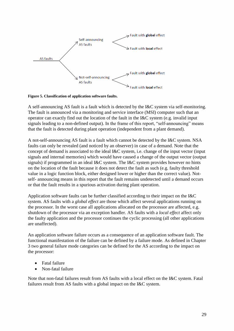
Figure 5. Classification of application software faults.

A self-announcing AS fault is a fault which is detected by the I&C system via self-monitoring.

The fault is announced via a monitoring and service interface (MSI) computer such that an

operator can exactly find out the location of the fault in the I&C system (e.g. invalid input

signals leading to a non-defined output). In the frame of this report, “self-announcing” means

that the fault is detected during plant operation (independent from a plant demand).

A not-self-announcing AS fault is a fault which cannot be detected by the I&C system. NSA

faults can only be revealed (and noticed by an observer) in case of a demand. Note that the

concept of demand is associated to the ideal I&C system, i.e. change of the input vector (input

signals and internal memories) which would have caused a change of the output vector (output

signals) if programmed in an ideal I&C system. The I&C system provides however no hints

on the location of the fault because it does not detect the fault as such (e.g. faulty threshold

value in a logic function block, either designed lower or higher than the correct value). Not-

self- announcing means in this report that the fault remains undetected until a demand occurs

or that the fault results in a spurious activation during plant operation.

Application software faults can be further classified according to their impact on the I&C

system. AS faults with a global effect are those which affect several applications running on

the processor. In the worst case all applications allocated on the processor are affected, e.g.

shutdown of the processor via an exception handler. AS faults with a local effect affect only

the faulty application and the processor continues the cyclic processing (all other applications

are unaffected).

An application software failure occurs as a consequence of an application software fault. The

functional manifestation of the failure can be defined by a failure mode. As defined in Chapter

3 two general failure mode categories can be defined for the AS according to the impact on

the processor:

Fatal failure

Non-fatal failure

Note that non-fatal failures result from AS faults with a local effect on the I&C system. Fatal

failures result from AS faults with a global impact on the I&C system.

30

In addition, two general failure mode types can be defined for the AS according to the impact

of the fault on the output signal:

Passive failure leads to an unavailability of the output signal, i.e. failure to actuate the

I&C function on demand.

Active failure leads to the spurious actuation of the I&C function.

Active failures occur when outputs change their value or state and lead consequently to a

spurious actuation. A spurious actuation can result in an

Unintended actuator movement (e.g. start or stop of a pump, opening of a valve)

Unintended command termination (e.g. clearing a command, leading to interruption of

an already initiated action, e.g. interruption of the opening of a valve).

For the analysis of spurious actuations it is convenient to consider the state of the plant, at

which the spurious actuation occurs. If the plant operates under normal operating conditions, a

spurious actuation caused as a result of an I&C failure results in an initiating event. If the

spurious actuation occurs in more than one division (e.g. as a consequence of a software fault)

the event can be classified as a common cause initiator (CCI). In this case the triggering

events are the signals processed under normal operating conditions of the plant. For faults

triggered during normal operation, the trigger could be also independent random effects, such

as hardware failures, time, and maintenance intervention. In this case the emission of spurious

signals induces the initiating event.

The second possibility is that the spurious actuation of an output signal is triggered by signals

acquired from the plant during an independent initiating event (e.g. spurious emission of a

stop signal to a pump which is needed to control a transient). In this case the spurious signals

are emitted after the initiating event occurred.

Regarding active failures the analysis presented in this report focuses on the emission of

spurious signals after the occurrence of an initiating event in the plant, e.g. during a transient.

Special interest is given to spurious actuations which impede the fulfilment of the required

I&C function to control the initiating event.

5. Analysis of operating experience

This chapter presents the use of the operating experience accumulated by digital I&C systems

implemented in the TELEPERM® XS (TXS) platform developed at AREVA to assess

software failures. The operating experience for TXS is based on an assessment of the non-

conformance reports (NCR) database until end 2013 (AREVA, 2014). The historical data

include the operating experience with the TXS platform installed in more than 60 nuclear-

related plants worldwide during commercial plant operation. These I&C systems are

permanently in operation, are broadly monitored, and have been working reliably and

accumulating applicable operating experience for over thirteen years.

In the next chapters the TXS operating experience for assessing system and application

software is presented.

31

5.1 Assessment of system software failures

5.1.1 TXS operating experience

The assessment of system software using the TXS operating experience has been considered

in (Bäckström et al, 2014). The triggers “temporal effects” and “faulty telegrams” are

identified in (Bäckström et al, 2014) as relevant initiators of system software common cause

failures. In Table 3 the failure rates associated to these triggers are listed, together with the

observed failures in operation until end of 2013. The failure rates are calculated using the one-

stage Bayes model

T

n

2

12 ,

where n is the total number of failures in operation and T is the accumulated operation time of

the corresponding reference group.

Table 3. Assessment of system software CCF triggering mechanisms using the TXS operating experience

CCF triggering

mechanism

Latent fault

location

Failures

in

operatio

n

Accumulated

operation

time

[h]

Failure

rate

[1/h]

Event

duration

[h]

Failure

probability(1)

SyS AS DCS

Temporal effects x 0 6.5E+6 7.8E-8 - 1.9E-6

Faulty telegrams x x 3 6.5E+6 5.4E-7 0.25 1.3E-5

Same system state/same

signal trajectories x x

0 6.4E+7 7.8E-9 - 1.9e-7

(1) Calculated considering a mission time of 24 hours.

Note that a mission time of 24 hours is considered in Table 3 to calculate the failure

probabilities of system software failures (self-announcing – fatal – failures). This assumption

is in-line with the PSA where a time frame of 24 hours is considered to analyse initiating

events. At time t=0 the initiating event takes place and its development is analysed in the PSA

for 24 hours (at t=24, the analysis ends). During this mission time (assumed to 24 hours) the

I&C functions are required to control the initiating event. In the case of the system software,

which operates continuously, it is required that no failure takes place during this mission time.

The mission time model estimates conservative failure probability of system software. This is

because the downtimes resulting from the observed failures are very short (approx. 15

minutes, see AREVA, 2015). The mission time approach covers however the case of a double

fault. If the same exception happens at least twice within approx. 5 minutes the processor

remains shutdown.

5.1.2 Reliability assessment of SyS software

Based on the outline of the failure modes in section 4 and the operational history presented in

Section 5.1.1, it is possible to estimate the SyS related faults.

The 1SS-DCU fatal CCF is estimated directly based on the operating experience for the TXS

system. The estimate is based on order of magnitude, rather than being considered an exact

estimate. The mission time is considered to be the normal mission time considered in a PSA –

24 hours. This must be considered conservative, since failures in the RPS at the end of the

sequence are far less critical than early failures (due to response time).

32

P(1SS-DCU fatal) = P(case 2b) = 2b Tm = 5.4E-7 24 = 1.3E-5 1E-5

Failure of a subsystem, 1SS-SyS fatal CCF is estimated in a similar manner.

P(1SS-SyS fatal) = P(case 2a) = 2a Tm = 7.8E-8 24 = 1.9E-6 2E-6

The failure mechanisms causing faults 2a (triggered by temporal effects) or 2b (triggered by

faulty telegrams) affect only one subsystem and for this reason are judged not to be relevant as

a basis for CCF between sub-systems (AREVA, 2014). As discussed in Chapter 4.1 failure

mechanisms affecting both subsystems are only limited to processors with the same system

software subject to the same internal system states or to application software subject to the

same signal trajectories and additional failure of fault propagation barriers (between

subsystems or between system and application software). For PSA purposes a correlation of

both subsystems caused by this failure mechanism cannot be completely ruled out, even

though the correlation is very weak if sufficient diversity in the application software is

considered in the design.

The failure mechanism affecting one complete subsystem has not been observed for the TXS

platform, not to mention the simultaneously failure of both subsystems. This is because

measures against correlation of both subsystems are taken into consideration in the TXS

design.

The failure probability of the complete system (P(SYSTEM-SyS fatal), see case 1 in Table 1)

is estimated considering a correlation factor between both subsystems and the probability

estimated for failures triggered by the same system states/signal trajectories (case 3, see Table

3), which affect at most a group of computers of one subsystem with the same system and

same application software. Assuming sufficient diversity of the application software in both

subsystems a correlation factor (β) of 0.01 is tentatively assumed for the estimation of the

failure probability of the complete system:

P(System SyS fatal) = P(case 3) β = 3 Tm β =

7.8E-9/h 24 h 0.01 = 1.9E-9 2E-9

Note that the correlation factor is a function of the diversity of the application software in both

subsystems. If sufficient diversity of the application software is ensured in the design, then the

correlation of both subsystems is very weak and can be modelled by a small correlation factor

(e.g. of 1%).

To summarise the SyS fault related basic events listed in Table 4 could be considered based

on the TXS experience.

33

Table 4. SyS fault related basic events.

SW failure event Tentative probability

SW fault 1:

SYSTEM-SyS fatal CCF 2E-9

SW fault 2a:

1SS-SyS fatal CCF 2E-6

SW fault 2b:

1SS-DCU fatal CCF 1E-5

5.2 Assessment of application software failures

The reference group to assess the application software failures using the operating experience

includes protection, limitation and control I&C (application) functions implemented on TXS

processors. These applications are of the same kind, i.e. implement nuclear application

functions, rely on the same system software, tool chain, libraries, and have been designed

under similar verification and validation (V&V) processes.

The time accumulated by these applications is estimated based on the operating experience of

TXS systems. For each I&C system the number of applications is estimated as shown in Table

5. These estimations are based on a conservative rounding of the total number of applications

found in I&C systems of new power plants, modernization of “Non-Konvoi” reactors and

Konvoi reactors.

Table 5. SyS fault related basic events.

I&C system Estimated number of application

functions for each I&C system

Nuclear instrumentation system 1

Control of process systems 5

Turbine control/protection 5

Reactor control 20

Reactor limitation 50

Reactor protection 50

Note that these estimations are conservative given the fact that the number of real applications

implemented in I&C exceeds the ones considered in Table 5.

The accumulated time of the application software reference group is calculated as follows. Let

i = 1, 2, …, K be the number of TXS-based I&C systems included in the historical data

base,

Ti be the operating (calendar) time of the I&C system i and

NAFi be the total number of application functions (AF) implemented in system i (estimated

according to Table 5).

The operation time accumulated by all application functions implemented in TXS-based I&C

systems can be calculated as:

TAF =

K

i 1

NAFi * Ti

Considering the TXS operating experience accumulated till end of 2013 from (AREVA, 2014)

the operating time for the application functions TAF is calculated to 1.7E+8 hours.

34

The contribution of the TXS applications to the total accumulated operating hours is shown in

Figure 6. Reactor protection system (RPS) applications provide approx. 67% of the

accumulated operating experience while control system (RCS) and reactor limitation system

(RLS) applications contribute with approx. 21% and 12%, respectively.

Figure 6. Contribution of TXS applications to the operating experience.

Note that the operating time accumulated by nuclear instrumentation systems, control of

process systems and turbine control/protection is assigned to the reactor control applications

given the similarity in the demand frequency of these applications.

Consideration of operating experience from one application function to assess failures of a

different application function relies on the assumption of exchangeability of failure and

demand events between different applications. This is a tentative first assumption made to

demonstrate the use of operational data. In future, other approaches will be considered. Under

the assumption that data from different applications can be pooled the consideration of the

operating experience of control and limitation applications to assess application software

failures of RPS is conservative. In order to justify this, the triggers and the AS faults from

these systems are compared.

The triggers depend on the operation profile of the system. The operation profile of RCS/RLS

is much more “explored” than the one of the RPS. This is because demands occur much more

often in RCS/RLS than in RPS. As a consequence, if there is a latent fault in the AS, there is

higher probability of triggering it in a RCS/RLS system than in the RPS system.

The amount of application software faults is considered to be correlated to the

Complexity of the software: the more complex the application, the higher is the

likelihood of latent faults and

Verification and validation process: the higher the system classification, the higher the

V&V requirements, the higher the likelihood to discover latent faults during the

system design phase.

The complexity of AS of RCS/RLS is (much) higher than the complexity RPS application

software. The classification of RPS is higher than RCS/RLS systems, i.e. RPS has higher

V&V requirements.

35

5.2.1 Applicability of the TXS operating experience

The applicability of the TXS operating experience to assess application software failures is

analysed in this chapter. According to the AS failures classification presented in Chapter 4.4.3

the possible failures resulting from AS faults within the reference group of computers

processing the same applications are:

The shutdown of the processor (fatal failure),

Unavailability of one I&C function (non-fatal, passive failure) or

Spurious actuation of one or several I&C functions (non-fatal, active failure).

The shutdown of a TXS processor occurs always as a consequence of software faults that are

detected by the system. If no failure treatment is available an exception handler is activated to

put the processor into a pre-defined fail-safe state (shutdown). The unavailability of one

application (no actuation) can occur either as a consequence of a detected fault or as a

consequence of fault not detected by the system. Spurious actuations occur as a result of a

design failure which cannot be detected by the system.

SA faults with fatal and non-fatal consequences are detected by the system itself before they

turn into a failure. These faults can be accurately tracked through the operating experience, i.e.

there is certainty that if a fault occurred the system detected it and provided information about

the nature and location of the fault. For this reason the TXS operating experience of redundant

processors can be accurately considered for the estimation of failure probabilities of self-

announcing software faults.

For NSA application software faults, the use of operating experience to estimate failure

probabilities is more limited. NSA faults are not detected by the system, i.e. the faults can

only be detected after turning into a failure, e.g. spurious actuation of a function. As

previously commented NSA failures result from faults in the functional requirement

specifications (FRS) or in the implementation of the functions and have passive (no actuation)

or active consequences (spurious actuation). Passive NSA failures result from faults that are

latent and can only be detected in case of a demand (e.g. exceeding of a threshold).

The use of the operating experience to assess NSA faults depends on the detectability of the

failure by an observer (operator). Design (latent) faults leading to a spurious actuation are very

likely to be detected by operators after the failure occurred (detection by plant behaviour).

There are more uncertainties associated to the detection of non-fatal passive failures that can

only be detected through the unavailability of a function after a demand.

During the accumulated operating experience the following uncertainties are associated with

the detection of non-fatal failures by an observer:

Uncertainties associated with the assumption that all failures on demand have been

detected and registered, given the fact that most of the reactor protection applications

have

o Diverse criteria to actuate a component (e.g. frequency and voltage for the

emergency diesel actuation)

o Diverse functions to actuate a component

o Diverse systems to fulfil a task (system function)

36

Uncertainties associated with the fact that all functions have been requested at least

once.

This last point is not critical for the TXS accumulated operating experience, given the large

amount of different TXS applications world-wide (more than 60 plants) and the accumulated

experience for more than 15 years.

In case the failure is detected/registered by the operator there is a further uncertainty

associated to the cause that originated the failure since no hints regarding the failure location

and nature are given by the I&C system to the operators. However it should be noted that a

great effort is invested to analyse the NCR to attribute I&C failures to the right causes

(AREVA, 2011).

Summarizing, fatal and non-fatal failures resulting from self-announcing AS faults (detected

by the system) and non-fatal active AS failures (spurious actuation detected by plant

behaviour) have a high associated certainty that the failures are detected and recorded in the

operating experience. For these failures the accumulated operating experience for the

reference group of redundant processors can be used to assess the failure probabilities.

The use of the operating experience to assess non-fatal passive failures resulting from NSA

faults has an associated uncertainty: the estimated probability reflects only those AS faults

which turned into a failure. NSA AS faults which did not result in a failure (e.g. because there

is a diverse actuation criterion) are not included in the operational history of TXS.

Note that all probability/failure rate estimations of application software failures using the TXS

operating experience correspond to estimations related to one application (I&C) function (and

not to an application software module).

5.3 Estimation of application software failures using TXS operating experience

Probabilities of application software failures are estimated in this chapter. The approach for

estimating AS failure probabilities combines the use of the operating experience with

engineering judgments for the estimation of failure fractions (see Section 5.3.1). The approach

presented in this report favours the use of AS failure fractions instead of AS fault fractions.

This is because failure fractions can be estimated using engineering judgments, whereas fault

fractions cannot. An observer can only notice failures of the AS (i.e. the consequence of an

AS fault) and get a feeling to make estimations of them. Operating experience shows the

history of the system failures and can be used for their assessment. On the contrary the

concept of AS faults is abstract and hard to estimate directly. For this reason the approach

proposed in this analysis assesses AS failures based on the TXS operating experience and on

expert judgments.

The assessment of AS probabilities for SA and NSA failures is presented in Section 5.3.2. In

Section 5.3.4 an assessment of probabilities of application software failure modes is

presented.

5.3.1 Estimation of failure fractions

In this chapter AS failure fractions are estimated with the aim of gaining insights about:

37

The fractions of total AS failures which are expected to have a global (fatal) or a local

(non-fatal) effect on the processor

The fractions of total AS failures which are expected to have a passive or an active

impact on the I&C function.

The decision tree shown in Figure 7 is considered to estimate the failure fractions.

Figure 7. Decision tree to estimate failure fractions of the TXS application software

The failure fractions are estimated for a general application. In reality there is a range of

different kinds of application functions, e.g. from the complexity point of view. The fractions

shown in Figure 7 are fractions of failures which can be interpreted as follows: Given 1000

SW failures, 900 failures are expected to be SA, 100 failures are expected to be NSA. From

the 100 NSA failures, 5 failures are expected to have global consequences (i.e. affect several

I&C functions) and 95 are expected to have no fatal consequences (local consequences, i.e.

only one I&C function).

The following failure fractions are of interest for the analysis:

Self-announcing vs. not-self-announcing failures

Global (fatal) vs. local (non-fatal) failures resulting from SA and from NSA faults

Active vs. passive failures resulting from local SA and from NSA faults.

SA failures can be triggered by signals during the normal operation of the plant and during an

independent initiating event (e.g. transient). This is justified by the fact that the complete

application code is run through in all cycles so that most of the potential SA faults are

expected to be discovered.

In this report NSA failures triggered in case of a demand of the function is analyzed, i.e. the

software is technically correct but it does not meet the functional requirement specifications.

Active failures during operation are not included in the analysis of NSA failures, since these

would lead to a common cause initiator (not studied in this report). Note that

38

For reactor control and reactor limitation systems demands occur during the normal

operation of the plant

For the reactor protection system a demand occurs during an initiating event (e.g.

transient).

The fractions shown in Figure 7 are justified in Appendix B, including an analysis of the

failure mechanisms of AS failures. These fractions are based on expert judgments and are

supported by the design features of the TXS system platform.

Note that the term application software refers in the next chapters to one application function

running on a processor.

5.3.2 Assessment of self-announcing application software failures

SA failures can be triggered by signals during the normal operation of the plant and during an

independent initiating event. For the assessment of SA failures the TXS operating experience

is directly considered to estimate the failure rate of AS.

The total probability of detected application faults is estimated considering that a total

operating time of approx. 1.7E+8 hours (until 31.12.2013) is accumulated for the AS

reference group (see Chapter 5.2). During this operating time no dependent failure has been

observed that can be categorized as a SA application software failure (AREVA, 2014).

The total failure rate of SA failures can be estimated using the one-stage Bayes model:

(AF SA) = AF

SA

T

n

2

12

where (AF SA): is the failure rate of SA failures of one application function [1/h],

SAn : is the total number of detected application software failures ( SAn = 0)

AFT : is the accumulated operation time of the reference group “all application

functions” (1.7E+8 hours, see Chapter 5.2).

The failure rate of one SA application software fault amounts to

(AF SA) = 2.9E-9/h

This failure rate can be interpreted as the rate of SA failures of one application function. The

total probability of detected AS failures can be calculated as the probability that the

application software fails during an independent initiating event , e.g. transient. As the I&C

system is in continuous operation, the probability of an AS failure occurring during the

transient can be assumed to be the probability of an AS failure occurring in the 24 hours

mission time associated to the event. Note that the mission time of 24 hours covers the

activation of I&C functions during the complete accident progression.

The probability of SA failures is calculated as:

P(AF SA) = (AF SA) * Tm

where Tm is the mission time. If a mission time of 24 hours is assumed the probability of SA

failures amounts to P(AF SA) = 6.9E-8.

39

The failure rates of SA failures with global and local effects (including passive and active

failures) are estimated next. The failure rates of SA application software failures are

summarized in Figure 8.

Figure 8. Estimation of failure rates of SA failures of the TXS application software

8

The failure rate of SA fatal failures resulting from the fault of one application is estimated

considering the total failure rate of SA application software failures and the failure fractions

estimated in Figure 7:

(AF SA fatal) = 0.05 * (AF SA fatal)

(AF SA fatal) = 1.4E-10/h

The probability of SA fatal failures can be calculated as

P(AF SA fatal) = (AF SA fatal) * Tm.

If a mission time (Tm) of 24 hours is assumed the probability of SA failures amounts to

P(AF SA fatal) = 3.5E-9.

The failure rate of SA non-fatal9 failures resulting from the fault of one application is

estimated in a similar way as considered in the previous chapter as:

(AF SA non-fatal) = 0.95 * (AF SA)

(AF SA non-fatal) = 2.7E-9/h

If a mission time of 24 hours is assumed the probability of SA failures amounts to

P(AF SA non-fatal) = 6.6E-8.

Based on the estimation of the non-fatal SA failures and of the failure fractions (see Figure 7)

the failure rate of SA active failures is calculated as

8 If the mission time model is considered the probability of SA failures for one application function can be

calculated as P = * Tm 9 Non-fatal means here: local effects, i.e. spurious actuation of one application function.

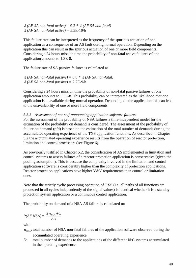
40

(AF SA non-fatal active) = 0.2 * (AF SA non-fatal)

(AF SA non-fatal active) = 5.5E-10/h

This failure rate can be interpreted as the frequency of the spurious actuation of one

application as a consequence of an AS fault during normal operation. Depending on the

application this can result in the spurious actuation of one or more field components.

Considering a 24 hours mission time the probability of non-fatal active failures of one

application amounts to 1.3E-8.

The failure rate of SA passive failures is calculated as

(AF SA non-fatal passive) = 0.8 * (AF SA non-fatal)

(AF SA non-fatal passive) = 2.2E-9/h

Considering a 24 hours mission time the probability of non-fatal passive failures of one

application amounts to 5.3E-8. This probability can be interpreted as the likelihood that one

application is unavailable during normal operation. Depending on the application this can lead

to the unavailability of one or more field components.

5.3.3 Assessment of not-self-announcing application software failures

For the assessment of the probability of NSA failures a time-independent model for the

estimation of the probability on demand is considered. The assessment of the probability of

failure on demand (pfd) is based on the estimation of the total number of demands during the

accumulated operating experience of the TXS application functions. As described in Chapter

5.2 the accumulated operating experience results from the operation of reactor protection,

limitation and control processors (see Figure 6).

As previously justified in Chapter 5.2, the consideration of AS implemented in limitation and

control systems to assess failures of a reactor protection application is conservative (given the

pooling assumption). This is because the complexity involved in the limitation and control

application software is considerably higher than the complexity of protection applications.

Reactor protection applications have higher V&V requirements than control or limitation

ones.

Note that the strictly cyclic processing operation of TXS (i.e. all paths of all functions are

processed in all cycles independently of the signal values) is identical whether it is a standby

protection system application or a continuous control application.

The probability on demand of a NSA AS failure is calculated to:

P(AF NSA) = D

nNSA

2

12

with

NSAn : total number of NSA non-fatal failures of the application software observed during the

accumulated operating experience

D: total number of demands to the applications of the different I&C systems accumulated

in the operating experience.

41

The total number of demands D accumulated until end of 2013 can be estimated as:

D = DRCS + DRLS + DRPS

where

DRPS are the total number of demands to applications of the reactor protection system (RPS)

DRLS are the total number of demands to applications of the reactor limitation system (RLS)

DRCS are the total number of demands to applications of the reactor control system (RCS).

The total number of demands to the application functions of the reactor protection, limitation

and control systems is estimated to (for details, see Appendix C):

DRPS = 3.4E+3

DRLS = 2.4E+3

DRCS = 7.0E+6.

Note that the DRCS >> DRLS and DRCS >> DRPS so that the total average number of demands can

be practically estimated with the average number of demands to the control systems

(D = DRCS).

Until end of 2013 no NSA application software failures have been observed ( NSAn = 0). The

probability of NSA non-fatal passive failures per demand is calculated to:

P(AF NSA) = 7.1E-8.

Based on this estimation and on the failure fractions (see Figure 7) the failure probability of

NSA failures with a global and local (non-fatal) effect is calculated as

P(AF NSA global) = 0.05 * P(AF NSA)

P(AF NSA global) = 3.6E-9

P(AF NSA non-fatal) = 0.95 * P(AF NSA)

P(AF NSA non-fatal) = 6.8E-8

As shown in Figure 9 NSA failures of the AS with non-fatal consequences can result in either

a passive failure (i.e. unavailability of the signal) or in an active failure (i.e. spurious signal).

The assessment of these failures is presented in the next chapters.

42

Figure 9. Estimation of probabilities on demand for one application function

Considering the estimation of NSA non-fatal failures and the failure fractions (see Figure 7)

the probabilities of NSA active and passive failures are calculated as

P(AF NSA non-fatal active) = 0.2 * P(AF NSA non-fatal)

P(AF NSA non-fatal active) = 1.4E-8

P(AF NSA non-fatal passive) = 0.8 * P(AF NSA non-fatal)

P(AF NSA non-fatal passive) = 5.4E-8

The estimated probabilities of NSA active and passive failures are conservative, especially for

RPS applications, for the following reasons:

Operating experience of the RCS and RLS has been considered for the probability

estimation of NSA non-fatal failures. Control and limitation applications are much

more complex and the V&V requirements are lower than the ones of the RPS. For this

reason, the probability estimated in this report corresponds to a medium/high software

complexity. This level of complexity is not present in the large majority of the RPS

applications. For this reason the estimates of NSA active and passive failures are very

conservative for RPS applications.

The failure probability on demand is estimated considering the failures occurred

during the TXS operation (nNSA = 0) and the total number of demands accumulated

during this operation time. The total demands are dominated by the demands to the

RCS (see Appendix A). The demands to the RCS are estimated in a conservative way

given the associated uncertainties (see Appendix A). Note that most of the RCS

applications are requested more often than the demands considered for this analysis.

The estimation of the number of application function implemented in each I&C system

contributing to the TXS operating experience is conservative. This result in a

conservative estimation of the accumulated time for the reference group of application

functions.

43

5.3.4 Assessment of the application software failure modes

The probabilities of AS failures estimated in the previous chapters are summarized in Figure

10, which shows the probabilities or the AS failure modes.

Figure 10. Estimation of probabilities and probability fractions for the failure modes of one application

function

The probabilities of the fatal AS failure mode can be estimated considering the following

equation:

P(AF fatal) = P(AF SA fatal) + P(ASF NSA global)

= (AF SA fatal) * Tm + P(AF NSA global)

Note that for the practical approach in PSA, it may be easier to model the fatal failure of the

processor caused by any of the applications implemented on it. The failure probability of the

processor caused by fatal failures of software can be calculated as

P(AF fatal total) = NAF * P(AFi fatal)

where NAF is the number of application functions located on the processor.

The probabilities of the non-fatal AS failure modes are estimated considering the following

equations:

P(AF non-fatal, no actuation) = P(AF SA non-fatal passive) + P(AF NSA non-fatal passive)

= (AF SA non-fatal passive) * Tm + P(AF NSA non-fatal passive)

P(AF non-fatal, spurious) = P(AF SA non-fatal active) + P(AF NSA non-fatal active)

= (AF SA non-fatal active) * Tm + P(AF NSA non-fatal active)

Note that for the calculation of the SA failures probabilities (P(AS SA fatal) and P(AS SA

non-fatal)) shown in Figure 10 a mission time of 24 hours is assumed. The probability

fractions (see blue numbers next to the branches in Figure 10) are estimated as:

P(AF fatal)/P(AS) = 0.05

P(AF non-fatal)/P(AS) = 0.95

44

P(AF non-fatal, spurious)/P(AS non-fatal) = 0.2

P(AF non-fatal, no actuation)/P(AS non-fatal) = 0.8

Note that these probability fractions are subject to the assumption of a 24-h mission time for

the estimation of the SA failure probabilities.

5.3.5 Estimation of failures for application software modules

This chapter discusses the use of the application software probabilities (for application

functions) based on operating experience to assess application software modules. The

example used here as reference for discussion is found in section 4.4.1.

The example shown in Figure 3 is considered to estimate the failure probabilities of fatal and

non-fatal failures of one AS module. Two AS modules can be defined for the application

software AS1 allocated in the APU: A&P-AS1 and APU-AS1.

In the next chapters fatal and not-fatal failures are analysed separately.

Estimation of fatal failures of application software modules

If a fault with fatal consequences occurs in one AS module, i.e. either in A&P-AS1 or in APU-

AS1, the APUs in all four redundancies shut down. If a fault with fatal consequences occurs in

the AS module VU-AS1, the Voter VU in all four redundancies shuts down.

For the estimation of the probability of fatal failures of one AS module, the following

considerations are taken into account:

For a first estimation the failure probabilities of all application software modules

included in an application function are assumed to be the same.

A fault in one AS module with fatal consequences leads to the failure (unavailability)

of the application function (to which the module belongs to) and to the failure of all

application functions allocated on the same processor.

The probability of fatal failures of one AS module can be conservatively estimated as

the fatal failure probability of the application function to which the module belongs to.

According to the considerations listed above, the fatal failure probability of one AS module i,

P(ASi fatal), is conservatively estimated as the failure rate estimated for one application

function:

P(ASi fatal) = P(AF fatal)

P(ASi fatal) = (AF SA fatal) * Tm + P(AF NSA global)

{ (AF SA fatal) = 1.4E-10/h, P(AF NSA global) = 3.6E-9}

If a mission time of 24 hours is assumed for the studied situation within the estimation of the

probability of SA fatal failures, then the fatal failure probability of one AS module is approx.

P(ASi fatal) = 7.0E-9

Note that for simplification reasons the same failure rates are assigned to software modules in

the APU and in the VU. The assessment of dependencies between application modules is not

45

relevant for fatal failures because the individual fatal failure of one application already leads

to the complete failure of the processor (all applications).

Estimation of non-fatal failures of application software modules

A non-fatal failure in one AS module is a fault for which the impact of the fault is restricted to

the faulty application module without affecting other applications allocated on the same

processor.

The complete software which defines an application (I&C function) in TXS can be

represented by the software modules A&P-AS, APU-AS and VU-AS10

(see Figure 3). For the

estimation of the probability of non-fatal (with active and passive consequences) failures of

one AS module, the following is considered:

For a first estimation the failure probabilities of all application software modules

included in an application function are assumed to be the same.

For non-fatal failures a fault in one AS module is assumed to lead to the failure of the

complete application function (unavailability of the function in case of a passive

failure, spurious actuation of the function in case of an active failure). This is the case

for processing modules (e.g. APU-AS1 in Figure 5) or for voting modules (e.g. VU-

AS1 in Figure 5). This is however conservative for failures of A&P software modules

(A&P-AS) in functions which involve more than one redundant (and diverse)

actuation criterion.

Non-fatal passive failures can be caused by SA and by NSA faults in the AS (see Figure 7).

Under the considerations presented in the previous chapter the probability of one AS module

ASi with passive consequences is conservatively estimated as the passive failure probability of

one application function:

P(ASi non-fatal, no actuation) = P(AF non-fatal, no actuation)

P(ASi non-fatal, no actuation) = (AF SA non-fatal passive) * T +

P(AF NSA non-fatal passive)

{ (AF SA non-fatal passive) = 2.2E-9/h , P(AF NSA non-fatal passive) = 5.4E-8}

Assuming a mission time of 24 hours, then the no actuation failure probability of one AS

module is approx.

P(ASi non-fatal, no actuation) = 1.1E-7

This probability can be interpreted as the contribution of the failure of one AS module to the

unavailability of an I&C function11

in all redundancies of the I&C system in which the

function is processed.

The probability of one AS module ASi with active consequences is conservatively estimated as

the probability of spurious actuation of one application:

10

Note that if reactor trip functions do not involve Voter units the complete application software can be

represented by the software modules AS-A&P and AS-APU. 11

In case other functions involve same faulty AS module the unavailability of these dependent functions has to be

postulated.

46

P(ASi non-fatal, spurious) = P(AF non-fatal, spurious)

P(ASi non-fatal, spurious) = (AF SA non-fatal active) * Tm + P(AF NSA non-fatal active)

{ (AF SA non-fatal active) = 5.5E-10/h, P(AF NSA non-fatal active) = 1.4E-8}

Assuming a mission time of 24 hours, then the spurious failure probability of one AS module

is approx.

P(ASi non-fatal, spurious) = 2.7E-8.

47

6. Reliability assessment of application software modules

6.1 Evidence on the reliability of application software modules

Figure 11 illustrates a Bayesian Belief Net (BBN) for quantification of software reliability

adapted from (Porthin & Holmberg 2013). This model includes three main pieces of evidence

which are proposed to be used in the quantification of probability of failure on demand (pfd)

of an AS: V&V level class, software complexity and observations from usage and tests. The

main rationale for the model is that development process and product quality affect the

reliability of the software, which in turn affects the amount of discrepancies observed during

usage and tests.

Figure 11. A BBN for assessing software reliability using V&V class, software complexity and usage and

test observations as evidence.

Design process quality is represented by the safety class of the software system, determining

required V&V measures. Product quality is represented by complexity of the software

solution, with the assumption that more complex software is more likely to fail. However,

complexity of software is not easy to define and measure accurately, so one may have to rely

on indicative complexity metrics or expert judgements. Still, receiving even indirect evidence

on the complexity of the software influences the beliefs on its reliability.

The observation node in the BBN includes all usage and test observations done after the

installation tests, e.g. maintenance and periodical tests are included in this node. Normally no

errors are found in the software at this stage, and known errors are fixed. The value of this

information depends on the representativeness of the observations with respect to the possible

and foreseeable state space of the software. Since this state space is huge, the

representativeness of tests and even of operation experience has traditionally been seen as

weak, and the evaluation would rather rely on the quality of software V&V measures.

6.2 V&V level

Within the nuclear domain the whole system is classified according to a safety class, for

example category A. To reach category A for RPS is a tedious process, and very expensive. At

least in Sweden and Finland, it is not considered likely that an RPS system based on one

platform can be claimed sufficient to fulfil the safety requirements of the NPP. Hence, a

separate system will be required. There is therefore no basis for assuming that some parts of

an RPS system can be claimed to be better validated than others and there is no driver to try to

increase the safety class requirements on the whole system – since there will anyway have to

be an independent system.

48

The table below defines the V&V classification that is used in the method outlined in this

report.

Table 6. V&V level.

V&V Safety class in nuclear (IEC 2009)

0 Non-nuclear safety

1 C

2 B

3 A

4 -

If it can be claimed that the V&V level is greater than corresponding to safety class A in the

nuclear domain, this can be represented by V&V level 4.

6.3 Complexity

6.3.1 General discussion

It is assumed in this work the number of faults in software is mainly dependent on two

metrics:

complexity

V&V grade.

In this work, a simple low/medium/high scale is used to represent the complexity of an AS

module. There is no unambiguously correct way to define the different complexity

classifications, even if every expert has already some intuition about what is complex and

what is not. While there is good agreement on distinguishing high from low complexity, the

line between low and medium complexity and medium and high complexity is not very clear.

The assessment is subjective. For instance, I&C experts and process engineers could have

different views, since I&C experts tend to focus on the use of memories and complex

computation, while process engineers pay more attention to complex input/output relations.

To estimate the complexity for software failure probability assessment, it is important to take

all the different viewpoints into account.

Nuclear automation software is typically designed using graphical tools where function blocks

are interconnected to form logic diagrams. From that graphic specification a code generator

builds the final source code. Hence, in this work, the complexity assessment is performed

based on logic diagrams.

6.3.2 Factors that affect complexity

In the following, different factors affecting the complexity of graphically specified software

are discussed.

Function blocks

Evidently the number and the complexity of function blocks affect the complexity of a logic

diagram. Complex function blocks typically use internal memories, perform complex

computation or include many inputs, outputs and parameters. If a logic diagram contains many

complex function blocks that are somehow connected or affect same output, the software will

likely belong to medium or high complexity category.

49

Interconnections between function blocks

The complexity of interconnections between function blocks affects the overall complexity

significantly, but it is difficult to measure. A diagram that includes only simple function

blocks, such as AND and OR, can also be moderately complex, if the number of function

blocks is large and interconnections are complex.

Generally, the more connections there are between function blocks, especially complex

function blocks, the more complex the software is. McCabe index (McCabe 1976) is one

option to measure the complexity of interconnections and software complexity in general, but

the source code is needed for the analysis. McCabe index measures the number of linearly

independent paths through the software’s source code. ISTec (Märtz et al. 2010) has a similar

approach to measure the complexity of interconnections. The counting of the number of

interconnections in a diagram is impractical unless it can be automated.

Feedback loops

The use of feedback loops increase the software complexity and therefore they do not appear

often12

in digital safety automation in NPP, but some examples exist. The generic logic

diagram of Figure A-2 contains a feedback loop. If a logic diagram includes a feedback loop

outside function blocks, its complexity category is commonly assessed as at least medium

unless the diagram does not contain practically anything else. Several feedback loops

combined with many inputs, outputs and complex function blocks can cause the diagram to

belong to the high complexity category.

Inputs and outputs

Having many inputs and outputs, especially of different types, complicates a software module

in a sense that it is difficult to use in combination with other modules. If inputs have different

types, they all need specific handling, which complicates the programming.

Upstream and downstream logic diagrams

If there are many logic diagrams that provide input to the analysed logic diagram and many

logic diagrams where the outputs of the analysed logic diagram lead to, the analysed diagram

is a part of a complex entity, and hence, using it is not easy. This factor correlates significantly

with the number of inputs and outputs.

6.3.3 Methods to assess complexity

The complexity analysis methods of ISTec (Märtz et al. 2010) and SICA (SImple Complexity

Analysis, Appendix A), are discussed briefly in this subsection and a generalizing approach

for the assessment of complexity based on them is put forward.

Institut für Sicherheitstechnologie (ISTec) developed its approach in 2010 to assess the

complexity of safety relevant software in nuclear power plants. An important aspect of

ISTec’s approach is its comprehensiveness and easiness of automation. SICA is an alternative

method that aims for simpler complexity analysis that an expert can perform by a short visual

assessment of a logic diagram. Both methods identify important parameters affecting software

12

If a feedback loop is used very often, like in the algorithm of a PI-controller, it is integrated into the function

block as an internal memory. Since it is frequently used and wrong connection is not possible, its contribution to

complexity is smaller than an explicit feedback loop and already taken into account by counting the number of

internal memories.

50

complexity.

6.3.4 ISTec

In ISTec’s approach each of the quantities listed in section 6.3.2 (except feedback loops) is a

component of a so-called complexity vector associated to a logical diagram. Engineering

judgment assigns hierarchic categories, which implicitly denote increasing degrees of

complexity, to each component of the complexity vector (see Table 7). The vector is then used

as an input for a Bayesian belief network (BBN) model which is used for the assigning the

logical diagram to a software reliability category.

Table 7: Hierarchic categories for each component of the complexity vector according to engineering

judgment (Märtz et al. 2010).

Label Description

Categories

Low Medium High Very high Extreme

high

K1 Number of function

blocks (FB) in LD FB ≤ 4 FB ≤ 12 FB ≤ 31 FB ≤ 101 FB > 101

K2 Number of input

signals (IS) in LD IS≤4 IS ≤ 8 IS > 8

K3 Number of output

signals (OS) in LD OS≤4 OS≤ 8 OS > 8

K4 Number of

upstream LD (FDI) FDI≤3 FDI ≤ 7 FDI > 7

K5

Number of

downstream LD

(FDO)

FDO≤4 FDO ≤ 6 FDO > 6

K6

Complexity of

interconnections of

FB (V-FP)

V-FP≤0.2 V-FP ≤ 0.4 V-FP > 0.4

V =

K7+K8

Variability (V) = P

+ IM (K7+K8) V=0 V ≤ 20 V > 20

K9 Complexity of FB

in LD (C-FB) C-FB≤2.5 C-FB ≤ 4.3 C-FB > 4.3

Note that the variability (V) is defined in Märtz et al. 2010 as the sum of parameters (P) and

internal memories (IM). These correspond to the complexity vector components K7 (number

of changeable parameters) and K8 (number of internal memories) of the ISTec method,

respectively.

An averaging of each of the components was performed in Märtz et al. 2010 based on logical

diagrams of a real application for RCLS. The results are summarized in Table 8.

As expressed above, these results for RCLS serve as a benchmark, or reference point, for

supporting the use of its operational experience for assessing probability of failure on demand

51

for other I&C systems.

Table 8: Averaging of data basis from a RCLS used in Märtz et al. 2010.

K1

Number

of FB

K2

Number

of

Inputs

K3

Number

of

Outputs

K4

Number of

Upstream

LDs

K5

Number of

Down-

stream LDs

K6

Normalized

complexity of

interconnect-

ions

K7+K8

Varia-

bility

K9

Complexity

of FBs

themselves

ISTec

Average 17.9 9.3 6 4.4 4.6 0.24 31.8 3.7

ISTec

Median

6.0 3.0 4.0 4.0 4.0 0.15 7.5 2.5

6.3.5 SICA

The SICA method prescribes rules to identify so called complex function blocks based on the

use of memory and the number of inputs, outputs and parameters. The number of connected

complex function blocks, the number of feedback loops and the sum of the number of inputs

and outputs are counted and the complexity category is determined by simple rules. The SICA

method is presented in detail in Appendix A.

6.3.6 Extended complexity vector

A simple extension of the ISTec’s complexity vector can be made by adding the number of

feedback loops (outside function blocks) of SICA as a component of the complexity vector. In

general, whenever a factor is found which affects the complexity of a diagram, it can be added

to the complexity vector, together with criteria assigning ranges of the factor to hierarchic

categories. On the other it can be beneficial to keep the number of explanatory variables

minimal, as usually aimed at in regression models.

6.3.7 Examples

Five generic examples of application functions for RPS are presented in Figure 12. ISTec and

SICA complexity factors are calculated for each of them. It is an expectation for RPS that they

should have a simple design and therefore it is expected that their complexity is lower than

that of RCLS.

52

Measurement

min

SGLW_MIN1

2 out of 4

Actuation

Internal

signals

out

Internal

signals

in

Logical

diagram 1

1

Measurement 1

min

SGLW_MIN1

2 out of 3

min

SGLW_MIN1

min

SGLW_MIN1

Measurement 2 Measurement 3

Actuation

Internal

signals

out

Internal

signals

in

Logical

diagram 2

2 out of 3

Internal

signals

out

Internal

signals

in

2 out of 3

Internal

signals

in

2 out of 3

Internal

signals

out

Internal

signals

in

1

Push

button 1

Push

button 2

1

1

S1 R

300 s

Internal

Criterion 2

Internal

Criterion 1

Actuator

1

Actuator

2

Actuator

3

Logical

diagram 3

Flip-flop

1

R S1

1

R S1

1

1

200 s

t 040 s

Push

button 1

Push

button 2Push

button 3

Push

button 4

Internal

Criterion 2

Internal

Criterion 1

Internal

Criterion 3

Internal

Criterion 4

Internal

Criterion 5

Actuator

1

Actuator

2

Internal

signal

Logical

diagram 4

Flip-flop

Flip-flop

Delay

1

1

1

1

1

min

RCLP_MIN4

2 out of 4

min

RCLP_MIN4

2 out of 4

1

130 s

Internal

Criterion 2

Internal

Criterion 1

Internal

Criterion 5

Internal

Criterion 3

Internal

Criterion 4

Internal

Criterion 6

Internal

Criterion 7

Actuator

Internal

signal 1

Internal

signal 2

External

signal

Process

Variable

A

Process

Variable

B

Internal

signals

out

Internal

signals

in

Internal

signals

in

Internal

signals

out

Logical

diagram 5

Figure 12: Generic logic diagrams

53

The rules for assignment to the hierarchic categories of ISTec (see Table 7) are applied to the

diagrams in Figure 12. SICA inspired K10 component is also evaluated. The results are

summarised in Table 9 and one can see that lower complexity factors dominate the logical

diagrams. Furthermore, comparing Table 8 and Table 9 one sees that those typical RPS logic

diagrams are indeed less complex than the ones in RCL I&C systems.

Table 9. Assignment of hierarchic categories to the components of the extended complexity vector of

typical RPS logic diagrams (green=low, yellow=medium, red=high).

K01 K02 K03 K04 K05 K06 V =

K07+K08 K09

K10

(feed-

back

loops)

LD01 2 1 1 3 3 0 6 3.640 0

LD02 8 3 1 9 6 0 18 3.241 0

LD03 4 2 1 2 0 0 7 2.433 0

LD04 9 4 1 5 1 0 11 2.118 0

LD05 16 3 1 7 2 0 17 1.758 0

6.3.8 Assessment of complexity degree of a logical diagram

SICA assigns a complexity degree (low, medium, high) to the whole logical diagram, while in

Märtz et al. 2010 such assignment is implicit, but hidden (Märtz et al. 2010 provides a

ranking). Since for the use of the BBN put forward in section 6.1 such complexity assessment

at the logical diagram level is necessary, it is interesting to investigate some possible rules for

mapping the complexity vector to a complexity degree.

Two point based methods are examined:

1- Average based comparison (ABC) – if the component of the LD complexity vector is

larger than the correspondent average of Table 8, one point is assigned to that

component. The points of all components are then summed up and the result denoted

by NPavg

2- Median based comparison (MBC)– if the component of the LD complexity vector is

larger than the correspondent median of Table 8, one point is assigned to that

component. The points of all components are then summed up and the result denoted

by NPmed

The mapping of these sums to a LD complexity degree obeys:

NP ≤ 3, LOWER complexity than the reference system (RCLS).

4 ≤ NP ≤ 6, SIMILAR complexity than the reference system (RCLS).

7 ≤ NP ≤ 9, HIGHER complexity than the reference system (RCLS).

54

It is a requirement from the standards that the RPS has a higher V&V grade than the RCLS

and this can be guaranteed by quality measures. (According to the IEC RPS is required to be

category A and RCLS is required to be category B.) If it is assumed that the average RCLS

would represent medium complexity, the interpretation would then be that LOWER indicates

low complexity, SIMILAR indicates medium complexity and HIGHER indicates high

complexity. Do note that SICA in the table below is not a relative estimate.

Table 10: LD complexity degree of the typical RPS logic diagrams according to SICA and ABC and MBC

point based methods.

SICA ABC MBC

LD1 LOW LOWER LOWER

LD2 LOW LOWER SIMILAR

LD3 LOW LOWER LOWER

LD4 LOW LOWER SIMILAR

LD5 LOW LOWER SIMILAR

In Table 10 the assessment of the LDs complexity using SICA, ABC and MBC is shown.

SICA and ABC rate all typical RPS LDs as of low complexity. The MBC on the other hand

gives that some LDs are of similar complexity to the reference system. As it is well known,

neither the average nor the median can alone unambiguously denote the typical behaviour of a

sample. However, taken both into account, one can affirm that the typical RPS logic diagrams

are simpler than the ones of the RCLS (given that the examples examined are representative

for RPS LDs).

6.4 Estimation of probabilities of AS modules

The software fault probability for an application software is hard to estimate. As shown in

Section 4.4, the application software fault can be defined using a number of fault parameters.

Normally the failure data available for software faults are not given on this level of detail. In

fact, it is hard to find any collection of failure data.

In the PSA model, the following quantities are needed

fatal failure rate (case 3) of AS modules

non-fatal failure rate of AS modules leading to failure to actuate (case 4-1)

non-fatal failure rate of AS modules leading to spurious demand (case 4-2)

According to the BBN model of Figure 11, the prior probability of the pfd given by the V&V

and complexity could be updated by operational data discussed in Section 5.3. It is far from

straightforward how this should be done. In this report we suggest two possible approaches as

the basis for the Bayesian process.

We call the first approach Failure announcing based estimate. In this approach we use the

observations of SA and NSA failures as the basis for the estimations. The second approach is

to directly use fatal and non-fatal failures as the observations/estimations. This alternative is

referred to as the Failure mode based estimate.

55

These two approaches are described below.

6.4.1 Failure announcing based estimate; SA and non-SA estimation

The failure announcing based estimate is based on the observations (evidence) of SA and

NSA failures. This information is then used to update priors for each type of failure.

When the Bayesian update has been performed, these estimates then need to be split using

fractions in fatal failures, non-fatal passive failures and non-fatal active failures.

Since the available data are very scarce (no known failures of application software), the priors

are tentatively developed based on current estimates used in the PSA today. The purpose is to,

in case there are no observations, derive in estimates that are in the same range as used in the

PSA. The priors then also need to consider that the current numbers in PSA are for I&C

functions rather than for AS module.

NSA failures, pfd

NSA failures are failures that manifest at demands13

, and hence they are comparable to the

failure probabilities that are used in the PSA. Some proposed and used failure probabilities for

AS function in PSAs are 1E-6 - 5E-5 (Jänkälä, 2010, Authén et al. 2010b, Enzinna et al.

2009). These probabilities are however not well defined compared to the proposed approach

in this report and are to some extent covering the different failure modes outlined in this

report (SyS failure modes, fatal failures and non-fatal failures).

An estimate of the mean pfd for NSA failures, which is disregarding from the different failure

modes (Case 1, 3, 4) and conservatively assuming the whole probability for NSA failures,

could then be 1E-5 for an AS function. The data does not separate different complexity

classes, but assuming that the RPS is of medium to low complexity, the value is considered

representative for medium complexity. The V&V level is 3, since this is category A software.

The approach suggested in this report is subdividing the AS function into AS modules. This

has to be taken into account, when the prior for AS modules is defined. An estimate of the

amount of AS modules that form an AS function is about 5–10. To account for this, the

baseline is lowered by a factor of 10.

Hence, using V&V equal to 3 and medium complexity software as the basis, the proposed

mean value of the prior would be:

E[PNSA| F] = 1E-6 * F

Where F is a shaping factor.

The prior is assumed to be a beta distribution Beta(,) with the above mean, and with an

of 0.5 and β = (1 – mean value) / mean value to represent a wide distribution. The prior

suggested above ranges (for medium complexity and V&V=3) from approximately 4E-9 to

4E-6 (5th

and 95th

percentile respective).

13

An NSA failure could potentially also generate a common cause initiator in case of a spurious activation during

plant operation, but this is not studied in this report.

56

In this approach it has also been considered reasonable that the difference in baseline failure

probability is a factor of 10 between high and medium respectively between medium and low

complexity software. It is also claimed that, similar to the IEC 61508, it is reasonable to

consider a factor of 10 between each V&V class.

The factor F is presented by the table below.

Complexity

High Medium Low

V&V 0 10000 1000 100

1 1000 100 10

2 100 10 1

3 10 1 0.1

4 1 0.1 0.01

SA failures, rate

SA failures will manifest themselves as soon as the failure occurs, and they are handled by the

software error handler. This type of failure could result in an unavailability of the AS module

(no-signal) or a spurious signal during the transient depending on how the error handler is set

up. A part of the SA failures could also lead to common cause initiators, CCIs, if the SA is

occurring during operation of the plant. CCIs are not discussed further in this context here.

The proposed tentative estimate of the prior is based on the assumption that the failure

probabilities used in PSA (discussed in previous section) could be caused by the probability

that a SA failure is occurring during the transient. In the PSA, a normal transient time

(mission time) is 24 hours.

This would mean that for a case with V&V = 3 and medium complexity the prior failure rate

would be estimated to 1E-6/24 5E-8/h.

The mean value of the prior for the SA failures would then be:

E[λSA | F] = 5E-8/h * F

Where F is a shaping factor presented in previous section with the same reasoning.

The prior is assumed to be a gamma distribution (,)14

with the above mean, and with an

alpha of 0.5 and = / mean value to represent a wide distribution. The prior suggested

above ranges (for medium complexity and V&V=3) from approximately 2E-10 to 2E-7 (5th

and 95th

percentile respective).

14

Using the parameterisation defined by the density function:

57

Quantification of the failure modes for the PSA

The evidence that is collected is the operational experience of SA and NSA failures. This

could be interpreted as failures identified by the system (SA) and failures discovered by the

operator (NSA). Thereby, it will only be possible to discover NSA failures when there is a

demand and the operator expects an action (or if a system is erroneously started – but it will

be hard to judge the demand rate in this case).

The observations need to be appropriately pooled, so they can be considered representative for

the data they are said to represent. It follows from the method that observations must be

separated in V&V and complexity classes. But it remains an open question how the

observations within one specific class should be pooled. For instance, can data from AS

modules with different FRS be pooled or is it appropriate to pool AS modules with high

demand rate with AS modules that have infrequent demand rate? The pooling assumption will

be an important assumption made by the analyst using the method.

When the posterior distribution has been calculated (for each group of AS modules), then

PNSA and λSA is available. This data is not directly useable in the PSA, and needs to be

transferred into the failure modes in the PSA (case 3, case 4-1, case 4-2). This step is achieved

by using split fractions. The tentative fractions used in this process are presented in Figure 13.

These are based on the fractions estimated by AREVA for TXS (see further section 5.3 and

justification in Appendix B).

SA (rate)

or

NSA (pfd)

Fatal failures

type 3

Non fatal failures

type 4

Active failure,

spurious signal

type 4-2

Passive failure.

no signal

type 4-1

0.05

0.95 0.2

0.8

Figure 13: Tentative split fractions

The estimate of the probabilities for the failure modes of one AS module in the PSA is:

P(Fatal) = 0.05 * PNSA + 0.05 * λSA * Tm

P(No signal) = 0.95 * 0.8 * PNSA + 0.95 * 0.8 * λSA * Tm

P(Spurious signal) = 0.95 * 0.2 * PNSA + 0.95 * 0.2 * λSA * Tm,

Where Tm is the mission time relevant for the AS module in the PSA.

All fatal failures on a processor are modelled in one and same basic event, which means that

all fatal failures on a processor shall be summed into one estimate.

The failure modes for no signal and spurious signal for AS modules are typically represented

by individual basic events for each failure mode and AS module.

58

Discussion

This approach could facilitate the observation process of failures, since it is subdivided in

failures that are expected to be observed during operation and failures that can only be

observed at demand.

Some challenges with the approach are:

Since the approach is not directly estimating the data that will be used in the PSA, it

relies on a very clear definition of fractions, and proper estimation of fractions, which

will be applied on the posterior. The above suggested fractions are to be considered as

tentative. For time being, we have only zero-failure data and it is therefore difficult to

validate the applicability of the taxonomy and reasonability of the fractions.

It is an open question how the pooling process of AS modules shall be performed.

The estimate of fatal failures for each AS module will require mapping of all AS

modules on a processor. This is needed to be able to calculate the fatal failure

probability of a processor, as a sum of the fatal failure probabilities of the AS modules

operating on the processor. This may be a tedious task, which could also lead to

overestimation of the fatal failure probability.

6.4.2 Failure mode based estimate; fatal and non-fatal failures

The approach directly estimates fatal failures and non fatal failures, without a need for expert

judgement on split fractions between these categories. The approach may also help in the

classification of failures, as the classification of SA and NSA failures is not evident if failures

happen at a demand. The failure mode based approach overcomes both of these questions.

The difference between the first and second approach is the estimation of fatal failures, since

the non-fatal failures follow a similar process as described in previous section.

Fatal failures

Since any fatal failure of a module has the same effect from the point of view of a processor

(APU/VU), the fatal failure rate could be directly estimated at the processor level. We assume

that all processors are similar from the point of view of a fatal failure. We might later consider

grouping them in different categories, if we can see that there are significant differences with

regard to number of modules, degree of complexity and degree of V&V between the

processors.

The benefit of this approach is to simplify the data analysis, since it can be done at the

processor level and it provides numbers that can be directly used. It should be further noted a

fatal failure (case 3) during normal operation would cause an initiating event. It would be a

common cause initiating event. The estimate for the failure rate is also an estimation of CCI

frequency.

AREVA has analysed data from about 150 processor-years of NPPs with digital safety I&C

with no fatal failures. No other event of this kind is known and hence assuming no such

events, the order of magnitude of fatal failure should be less than 1E-3/yr on a processor level.

This means that prior mean failure rate during mission could be of order 1E-7/h per processor.

It is a matter of future research to analyse whether processor type specific priors can be

estimated (e.g. APU vs. VU, based on number of modules, degree of complexity of modules,

59

degree of V&V). Also further investigation of world-wide experience of fatal failures is

needed. The assessment of fatal failure-events and frequencies needs to be revisited later, too.

It can be noted that the total SA fatal failure rate assessed in Section 5.3.2 is about 3E-9/h per

module. The assessment 1E-7/h is slightly higher, when taking into account that the estimate

in Section 5.3.2 is actually on an I&C function level estimate.

Non-fatal failures at demands

For non-fatal failures the data analysis must be done at the I&C function or module level,

since the failure effect is module specific. This is more demanding since the generic operating

experience does not give much support.

This type of failure is probably mainly a matter of NSA failures. However, the approach of

estimating non-fatal failures at demand does not need to distinguish between SA and NSA

failures, since the approach is failure mode oriented. Per definition, the failures can be

identified only at demands, and the demand data is very scarce for many of the I&C functions.

For non-fatal failures the BBN approach with complexity and V&V attributes is suggested,

and it can be formulated in a shaping factor formula. The result can be updated by operating

experience if available. This process would basically follow the intentions of Section 6.4.1

with regard to NSA failures.

The obtained non-fatal failure probability can be then divided into to the failure modes ”no

signal” (4-1) and ”spurious actuation” (4-2) using e.g. the fractions suggested by AREVA.

Quantification

The quantification process follows the same type of quantification approach as described in

Section 6.4.1. However, the estimated entities in this approach are the fatal failures and the

non-fatal failures.

Fatal failures are tentatively estimated on processor level and are the same for all processors.

The non-fatal failures needs to be split into the relevant failure modes and are following the

split representing individual AS modules and failure mode.

Discussion

This approach would facilitate the estimate of especially fatal failures, since only one fatal

failure estimate is done. It will also remove the need for a discussion of observations at

demands related to whether the failures are SA or NSA. Since the fatal failure estimate is

performed on a high level, the focus in the approach would be on AS modules for no signal

and spurious signal.

Some challenges with the approach are:

The approach does not, in current form, differentiate between amount of processes

running on a processor and complexity of processes. How an increased level of detail

could be applied and the benefit of doing it should be evaluated later, compared to

analysis efforts needed and compared to uncertainties related to all estimates required

in a detailed analysis.

The outlined estimate of fatal failures does not, in its current form, consider fatal

failures from signal trajectories during a demand. We might try to use global demand

60

data to get some reference for an appropriate order of magnitude of probability of fatal

failure per demand.

We assume that all processes, from a fatal failure point of view, can be pooled. As far

as we have zero failure data, this is a critical assumption, which requires further work

to justify.

For non-self announcing failures, the challenges are the same as in section 6.4.1.

6.4.3 Examples

The examples are using the Failure announcing based estimate, which means observations are

based on SA and NSA failures.

Example 1

The observations by AREVA (see Section 5) are used as basis for the example. The same type

of pooling as used in section 5 is used here, hence it is assumed that all observations of SA

and NSA failures can be pooled. It is further assumed that all observations are assumed

relevant for category A and complexity class medium.

SA failures

Observed failures kSA = 0

Operational experience TSA = 1.7E8 h (assumed relevant for AS modules)

The mean prior failure rate for AS module is E[λSA] = 5E-8/h. The distribution of the prior is

assumed to be a gamma distribution, with parameters α = 0.5 and β = 0.5 / 5E-8/h = 1E7 h).

The Bayesian update yields following mean estimate:

E[λSA | kSA, TSA] = 0.5 / (1.7E8 h + 1E7 h) = 2.8E-9/h

NSA failures

Observed failures kNSA = 0

Observed demands nNSA = DRCS + DRLS + DRPS = 7E6 + 2.4E3 + 3.4E3 = 7E6

The mean prior failure probability for AS module is E[PNSA] = 1E-6. The distribution of the

prior is assumed to be a beta distribution, with parameters α = 0.5 and β = 0.5*(1 – 1E-6) / 1E-

6 = 5E5).

The Bayesian update yields following mean estimate:

E[PNSA | kNSA, nNSA] = 0.5 / (7E6+5E5) = 6.7E-8

Calculation of PSA failure modes

The estimates calculated above are transferred into relevant PFD estimates to be used in the

PSA assuming a mission time of 24 hours. These estimates are for one AS module. Note that

fatal failures for a processor shall represent all AS modules on the processor. (The formulas

are presented in Section 6.4.1.)

P(Fatal) = 0.05 * 6.7E-8 + 0.05 * 2.8E-9/h * 24 h = 6.7E-9

P(No signal) = 0.95 * 0.8 * 6.7E-8 + 0.95 * 0.8 * 2.8E-9/h * 24 h = 1.0E-7

P(Spurious signal) = 0.95 * 0.2 * 6.7E-8 + 0.95 * 0.2 * 2.8E-9/h * 24 h = 2.6E-8

61

Example 2

In this example it is assumed that 20%, 50% and 30% of the operational experience for SA

failures is representing high, medium and low complexity AS respectively. The NSA

operational experience for RPS is assumed to represent low complexity AS. In this example it

is not considered relevant to pool observations for RCS and RPS, based on the assumption

that high demand rate AS modules should not be pooled with low demand rate AS modules.

We are seeking the probabilities for the failure modes to be used for an RPS AS. There are ten

AS modules on the relevant processor, all with low complexity.

This estimate can be considered as the basis for the example model used in the DIGREL main

report (Authén et al. 2015).

SA failures

Observed failures kSA = 0

Operational experience TSA = { 30% of 1.7E8 h } = 5.1E7

The mean prior failure rate for AS module is E[λSA] = 5E-9/h. The distribution of the prior is

gamma(0.5, 1E8 h).

The Bayesian update yields following mean estimate:

E[λSA | kSA, TSA] = 0.5 / (5.1E7 h + 1E8 h) = 3.3E-9/h

NSA failures

Observed failures kNSA = 0

Observed demands nNSA = DRPS = 3.4E3

The mean prior failure probability for AS module is E[PNSA] = 1E-7. The distribution of the

prior is beta(0.5, 5E6).

The Bayesian update yields following mean estimate:

E[PNSA | kNSA, nNSA] = 0.5 /(3.4E3 + 5E6) = 1E-7.

Calculation of PSA failure modes

The fatal failure probability for one AS module is estimated to:

P(Fatal) = 0.05 * 1E-7 + 0.05 * 3.3E-9/h * 24 h = 1.0E-8.

The fatal failure probability for the AS modules running on the processor is hence 1.0E-7 (10

AS modules of low complexity assumed). The failure probability to be used for the AS

module for non-fatal failure modes are calculated below.

P(No signal) = 0.95 * 0.8 * 1.0E-7 + 0.95 * 0.8 * 3.3E-9/h * 24 h = 1.4E-7

P(Spurious signal) = 0.95 * 0.2 * 1.0E-7 + 0.95 * 0.2 * 3.3E-9/h * 24 h = 3.4E-8.

62

6.5 CCF between related AS modules

Generally, the AS modules performing an identical function in redundant divisions are

assumed to be identical software modules. The conditional probability of CCF is 1, given a

fault in an AS module.

In addition to CCF between identical AS modules, it is worth considering CCF between

related AS modules. At least two kinds of relationships can form a potential to CCF:

use of same elementary functions

common functional requirements specifications.

With regard to the fault coupling by elementary functions, it is in principle possible to assume

fault in an elementary function module which would then be a common fault for more than

one AS module. However, the position of this report and method is that faults in elementary

functions are practically eliminated due to their being part of the rigorous verification and

validation of the system software. It is instead more likely that an AS fault is caused by a

wrong usage of complex elementary function. Thus, the main attention should be paid on the

assessment of use of complex elementary functions, and the fault coupling can be associated

with the coupling via common functional requirements specifications.

With regard to the fault coupling by functional requirements specifications, the practically

relevant case is possible CCF between two AS modules implementing same I&C function in

diverse subsystems. In a PSA model, the two AS module failure basic events appear under an

AND gate so that the CCF probability has a significant impact on the overall failure

probability of the safety function. There are numerous such examples in the current way of

designing safety I&C, since it is an overall requirement that the actuation of safety functions

should be accomplished by two different process parameters (e.g., temperature and pressure of

primary circuit).

The critical issue is the assessment of CCF between AS modules AS-x-1 and AS-x-2, which

are part of the implementation of the same I&C function in different subsystems of RPS.

Conservatively, the conditional probability of CCF could be assumed to be 1. Optimistically,

no dependency is assumed. A realistic assessment is somewhere between, where?

63

7. Summary of failure data evaluation process

Based on the software quantification process described this report (Section 4,Section 5.1.2 and

Section 6) can be summarized by Figure 14. The figure illustrates the different failures that are

considered for a process running on a processor within certain application software AS1. The

processor is running on the system software environment SubSyS1, which is a subsystem of

the SyS software (the complete system has two different subsystems). On the processor there

are several application software running.

System

SyS software

Application

software AS1

SyS fault 1

Fatal failure,

SubSyS1

fault 2a, 1 SS

fatal failure

SubSyS1

fault 2b, 1 SS

fatal failure

DCS

Complexity

estimate AS1

V&V estimate AS1

AS1 failure

probability

AS1

Fatal failure

probability

AS1 No

signal

failure

probability

AS1

Spurious

failure

probability

Figure 14. Summary of the failure data assignment process

The system software failure modes are considered to be generic for the system, and subsystem

failures are generic for the parts of the system where the subsystem software is used. The

failure probabilities for the SyS and SubSyS are estimated based on operational history.

The application software is studied with regard to complexity and the level of V&V. Thereby

an AS software failure probability can be estimated. This is then split into three failure

probabilities, fatal failure, no signal and spurious signal.

Figure 15 below presents the intended use of these faults in the model for the different failure

modes. When studying an individual failure mode for an application software it has to be

determined if:

The system, or subsystem, software fatal failure would cause the unwanted signal

If a fatal failure in this application software (or any other AS running on the same

processor) may cause the unwanted signal

64

Both of these faults are related to the configuration of the processes on the processor, i.e. the

definition of the safe states since a fatal failure will halt the processor – and unwanted signals

will be generated only if the safe state is causing an unbeneficial signal.

AS failures – No signal

Failure of the individual process AS1 + fatal failures of all AS if the configuration is such that fatal failures cause no

signal. If fatal failures are critical, then it should be the sum of fatal AS failures on the processor.

System failures – General failure modes

Fatal failures only relevant if they do not cause the expected signal

Failure affecting

one AS1 on a

processor with n

AS

AS1

Fatal failure

probability

AS1 No

signal

failure

probability

ASn

Fatal failure

probability++

AS failures – Spurious signal

Failure of the individual process AS1 + fatal failures of all AS if the configuration is such that fatal failures cause

spurious signal. If fatal failures are critical, then it should be the sum of fatal AS failures on the processor.

AS1

Fatal failure

probability

ASn

Fatal failure

probability++

AS1

Spurious

failure

probability

SyS fault 1

Fatal failure,

SubSyS1

fault 2a, 1 SS

fatal failure

SubSyS1

fault 2b, 1 SS

fatal failure

DCS

Figure 15. Use of faults in the model for different failure modes

A complete CCF is considered between all units using the subsystem and system software

respectively. The failure mode shall be modelled so that fatal failures are represented correctly

with regard to the signals from the system.

Note that the fatal failure of application software is represented either for the no signal

scenario or the spurious signal scenario.

CCF between different AS modules should be considered. Full correlation (CCF=1) is

assumed between redundancies. Dependencies between software modules shall be represented

explicitly and there is hence no need for CCF representation. CCF for application software

that are very similar may be relevant to consider.

65

8. Case study with the example PSA model

In the DIGREL project, an existing simplified PSA model has been complemented with fault

tree models for a four-redundant distributed protection system in order to study and

demonstrate the effect of design features and modelling approaches. The model has been used

to test the effect of different levels of modelling detail, CCF modelling, fail-safe principle and

voting logic. The example PSA-model represents a fictive boiling water reactor (BWR),

which has four-redundant safety systems. For details, see (Authén et al. 2015). In this report

only the modelling of software failures is discussed.

Generally, same failure modes (types 1, 2a, 2b, 3, 4a and 4b) are considered in the model and

the same failure probabilities are used as suggested in this report. The fault trees for I&C have

been structured in hierarchical manner starting from the actuator down to measurements.

Details are described in (Authén et al. 2015). An example is given in Appendix D to

demonstrate the appearance of software basic events.

Failure to start a safety critical pump is considered (e.g. emergency feedwater (EFW) pump).

Generally, the software faults can be modelled parallel to hardware faults with same failure

effects. It is practical to distinguish between fatal SW failures which affect all outputs of the

unit and non-fatal SW failures which have I&C function specific effects.

It should be noted that depending on the fail-safe principle it must be decided whether

detected or undetected failure modes need to be considered. In this example, it is assumed that

detected failure of voting unit will inhibit the actuation, but detected failure of APU will be

treated as an actuation of EFW start by the voting unit.

The results of the example PSA show that software faults have a significant impact on the

overall result. Software faults in total have a fractional contribution of about 5%. For details

on risk importances, see (Authén et al. 2015). It can be concluded that software faults in

general have a non-negligible effect on the results and should be considered in a digital I&C

PSA. Quantification of software faults and the assessment of the degree of diversity between

subsystems can therefore be significant from the overall PSA results point of view.

66

9. Conclusions

The advent of digital I&C systems in nuclear power plants has created new challenges for

safety analysis. To assess the risk of nuclear power plant operation and to determine the risk

impact of digital systems, there is a need to quantitatively assess the reliability of the digital

systems in a justifiable manner. Due to the many unique attributes of digital systems, a

number of modelling and data collection challenges exist, and consensus has not yet been

reached. It is however agreed that software failures are relevant events, which should be

considered probabilistically in PSA.

Currently in PSA, computer-based systems are mostly analysed simply and conventionally.

The conventional failure modes and effects analysis and fault tree modelling are utilized. The

survey of literature and PSA shows that software failures are either omitted in PSA or

modelled in a very simple way as CCF related to the application software of operating system.

It is difficult to find any other basis for the numbers used except the reference to a standard

statement that a failure probability 1E-4 per demand is a limit to reliability claims, which limit

is then categorically used as a screening value for software CCF.

In the OECD/NEA DIGREL task, a failure modes taxonomy was developed jointly by PSA

and I&C experts. At higher system and I&C unit level of abstraction there is no need to

distinguish between hardware and software. When level of abstraction is broken down into

smaller details, it becomes meaningful to define hardware and software modules and related

failure modes.

In order to simplify the failure modes taxonomy and yet keep it comprehensive, software

related failure modes can be simply defined by a) their location, i.e., in which module the fault

is, and b) their effect on I&C unit. For a processor the effect is either a fatal failure of the

processor (termination of the function and no outputs are produced) or a non-fatal failure

where operation continues with possible wrong output values. The consequence of a fatal

failure can be defined for processors running in reactor protection system, since the failure

behaviour is known. Outputs are set to supposedly safe values. The consequence of a non-fatal

failure can be related to the application functions implemented in the processor. In RPS, the

two main failure modes of a non-fatal failure are failure to actuate a specific I&C function and

spurious actuation of a specific I&C function.

There is a large number of possible combinations of software fault locations and affected I&C

units. Due to the diversity and redundancy principles, the number of cases can however be

reduced to a few relevant cases from the PSA modelling point of view:

1. Fatal failure causing loss of all subsystems that have the same System Software (Case

1).

2. Fatal failure causing loss of one subsystem

a. Fault is in System Software (Case 2a). The whole subsystem stops running and

outputs are set to 0.

b. Fatal failure in communication modules of one subsystem (Case 2b). The

voting units run and take default values.

3. Fatal failure causing failure of redundant set of I&C units, i.e, a set of acquisition and

processing units (Case 3a) or a set of voting units (Case 3b) in one subsystem.

67

4. Non-fatal failure associated with an application software module. The failure effect can

be a failure to actuate the function or a spurious actuation (Case 4). The fault can be in

the APUs or VUs.

Software reliability quantification will always be a controversial issue. In DIGREL project

different approaches have been reviewed and possible pieces of evidence have been explored.

In the proposed method, software reliability quantification depends on the type of the software

module.

Software fault cases 1 and 2 are associated with System Software, and operational data may

provide insight of the level of failure rate. In the TXS operating experience analysed by

AREVA, no failure of the System Software were found (cases 1 and 2a). Few cases of failed

communication (faulty telegrams) have been reported (case 2b).

Software fault cases 3 and 4 are associated with the application software modules. It is

assumed that a priori the failure probability can be correlated with two metrics: complexity of

the application software and the degree of verification and validation of the software. Degree

of V&V is related to the safety class of the software system. Complexity can be assessed by

analysing the logic diagram specification of the application software module.

The report suggests a numerical scheme to correlate between the metrics and failure

probability, in terms of a “shaping factor”. This approach is similar to the quantification

methods used in human reliability analysis. The resulting number is assumed to include all

failure modes (fatal failure, no actuation, spurious actuation). Expert judgement is considered

to estimate the fractions of different failure modes.

In principle, a priori estimates could be updated by operational data. In case of reactor

protection system, there are very few real demands during operation. On the other hand for

other safety related I&C systems, which can be implemented by same platform, there can be a

lot of demands, which opens an opportunity to use operational data. Such operating

experience has been analysed by AREVA assuming that the TXS operational experience from

different I&C systems can be pooled. A simple one-stage Bayesian estimation is considered in

the report to estimate failure probabilities of the application software.

The outlined approach to quantify software reliability must be seen principally as a

demonstration of the pieces of evidence needed for the quantification and the analysis steps

needed for such an assessments. The numbers obtained with the proposed quantification

method have not been validated, and there are a number of technical issues which require

further justification. Therefore the users of the report should primarily pay attention to the

failure modes and software fault cases suggested in the report. The numbers presented in the

report intend to demonstrate the quantification method, and they shall not be generically used

without detailed case-by-case justification. Estimation of probabilities will always be a vendor

and design specific task.

The method is not considered finalized. Remaining issues include:

Search for more justification of the definition of the software fault cases. The proposed

set of fault cases cover at least most relevant cases. The question is if some relevant

case is missed in this proposal.

68

Validation of the method versus real cases, operational data or expert judgements. The

method relies on several assumptions and expert judgements. Validation of it is a hard

task, but should be tried out. Data may provide some support. Expert judgements

techniques may be also used to check if the results provided by the method correspond

with experts’ judgements.

Benchmarking of the software quantification method with other quantification

methods. There are several alternative methods proposed for software reliability

quantification in the context of PSA. It would be useful to compare the approaches

both with regard to assumptions made and numerical values estimated.

Improved guidance on categorisation of complexity. Complexity is regarded as a

relevant indicator for the reliability of the application software module. It is possible to

analyse complexity be examining the logic diagrams, but the question is to define a

justifiable approach to classify complexity. It should be also noted that complexity

classification is dependent on the definition of the module, which can be done at

different levels of abstraction.

Search for more justification for the fractions assumed between different failure modes

of application software modules. The estimation of fractions are based on expert

judgements. Some arguments for the estimates are given in this report, but they may

require more back-up.

Search for more justification regarding the use of operational data for the failure rate of

System Software and communication unit software. A claim is made that only fatal

failures are relevant and that failure rates can be assumed to be generic (not plant-

specific). Counter-arguments can be made, but on the other hand non-fatal or plant-

specific failures may be assumed to be covered by the application software related

failures. The issue needs to be studied further.

Application of a two-stage Bayesian approach to utilize operational data from

application software modules. In the data analysis of this report, a one-stage Bayesian

approach is used. This approach relies on a strong assumption of exchangeability of

data for different modules. In a two-stage Bayesian approach, this assumption can be

made weaker. A two-stage Bayesian approach is used e.g. in T-book for conventional

nuclear components (T-book 2010).

Guidance to define application software modules and associated basic events in a real

PSA. The proposed approach can lead to a large number of basic events in a real PSA,

which can be impractical. Experiments are needed to see if it is practical to model

things in a detailed manner or if it is possible to do the modelling in a simplified

manner.

Guidance in CCF treatment between application software modules which have

common requirements specification.

69

10. References

AREVA, 2009. Quantitative Bewertung des Einflusses eines GVA auf die Unverfügbarkeit

von Leitsystemen in TELEPERM XS Gerätetechnik. Work Report NLR-G/2009/de/0001 rev.

A; AREVA GmbH.

AREVA, 2011. Managing operating experience with TXS. Report PTLC-G/2010/en/0046 rev.

A; AREVA GmbH.

AREVA, 2012. TXS Self-monitoring and fail-safe behavior from Core-Software Release

3.6.2 - Work Report PTLC-G/2011/en/0059 rev. A; AREVA GmbH

AREVA, 2013. TXS Computers CCF Assessment including Consideration of Spurious

Signals - Report PTLS-G/2013/en/0005 rev. A; AREVA GmbH

AREVA, 2014. Quantitative assessment of the influence of CCF on the unavailability of TXS-

Based I&C systems - Work report PTL/2014/en/0001 rev. A; AREVA GmbH

Authén, S, Björkman, K., Holmberg, J.-E., Larsson, J. 2010a. Guidelines for reliability

analysis of digital systems in PSA context — Phase 1 Status Report, NKS-230 Nordic nuclear

safety research (NKS), Roskilde.

Authén, S., Wallgren, E. & Eriksson, S. 2010b. Development of the Ringhals 1 PSA with

Regard to the Implementation of a Digital Reactor Protection System. In: Proc. 10th

International Probabilistic Safety Assessment & Management Conference, PSAM 10, Seattle,

Washington, June 7–11, 2010, paper 213.

Authén, S., Gustafsson, J., Holmberg, J.-E. 2012. Guidelines for reliability analysis of digital

systems in PSA context — Phase 2 Status Report, NKS-261 Nordic nuclear safety research

(NKS), Roskilde.

Authén, S., Holmberg, J.-E., 2013. Guidelines for reliability analysis of digital systems in

PSA context - Phase 3 Status Report, NKS-277, Nordic nuclear safety research (NKS),

Roskilde.

Authén, S., Holmberg, J.-E., Lanner, L. Tyrväinen, T. 2014. Guidelines for reliability analysis

of digital systems in PSA context –Phase 4 Status Report, NKS-302, Nordic nuclear safety

research (NKS), Roskilde. Draft

Authén, S., Holmberg, J.-E., Tyrväinen, T., Zamani, L. 2015. Guidelines for reliability

analysis of digital systems in PSA context – Final Report, NKS-xxx, Nordic nuclear safety

research (NKS), Roskilde. Draft

Bishop, P.G. & Bloomfield, R.E. 1996. A Conservative Theory for Long Term Reliability

Growth Prediction. In IEEE Trans. Reliability, 1996, 45(4): 550–560.

Björkman, K., Bäckström, O., Holmberg, J.-E. 2012. Use of IEC 61508 in Nuclear

Applications Regarding Software Reliability — Pre-study, VTT, VTT-R-09293-11

70

Björkman, K., Frits, J., Valkonen, J., Heljanko, K., Niemelä, I. Model-based analysis of a

stepwise shutdown Logic, MODSAFE 2008 Work Report, VTT working papers 115, VTT,

Espoo, March 2009, 42 p.

Bäckström, O., Holmberg J-E., Jockenhövel-Barttfeld M., Porthin M. and Taurines A. 2014.

Software reliability analysis for PSA - NKS-304, Nordic nuclear safety research (NKS),

Roskilde.

Bäckström, O. & Holmberg, J.-E. 2012. Use of IEC 61508 in Nuclear Applications Regarding

Software Reliability, Proc. of 11th International Probabilistic Safety Assessment and

Management Conference & The Annual European Safety and Reliability Conference, 25–

29.6.2012, Helsinki, paper 10-Th2-4.

Chu, T.L., Martinez-Guridi, G., Yue, M., Samanta, P., Vinod, G., and Lehner, J. 2009.

Workshop on Philosophical Basis for Incorporating Software Failures into a Probabilistic Risk

Assessment, Brookhaven National Laboratory, Technical Report, BNL-90571-2009-IR,

November.

Chu, T.-L., Yue, M., Martinez-Guridi, G. & Lehner, J. 2010. Review of Quantitative Software

Reliability Methods, Brookhaven National Laboratory Letter Report, Digital System Software

PRA JCN N-6725.

Dahll, G., Liwång, B. & Pulkkinen, U. 2007. Software-Based System Reliability, Technical

Note, NEA/SEN/SIN/WGRISK(2007)1, Working Group on Risk Assessment (WGRISK) of

the Nuclear Energy Agency, Paris.

Enzinna, B., Shi, L. & Yang, S. 2009. Software Common-Cause Failure Probability

Assessment. In: Proc. of Sixth American Nuclear Society International Topical Meeting on

Nuclear Plant Instrumentation, Control, and Human-Machine Interface Technologies,

NPIC&HMIT 2009, Knoxville, Tennessee, April 5–9, 2009.

Eom, H.-S., Park, G.-Y., Kang, H.-G. & Jang, S.-C. 2009. Reliability Assessment Of A

Safety-Critical Software By Using Generalized Bayesian Nets. In: Proc. of Sixth American

Nuclear Society International Topical Meeting on Nuclear Plant Instrumentation, Control, and

Human-Machine Interface Technologies, NPIC&HMIT 2009, Knoxville, Tennessee, April 5–

9, 2009

EPRI. 2010. Estimating Failure Rates in Highly Reliable Digital Systems. EPRI TR-1021077,

Electric Power Research Institute, Inc., Palo Alto, CA. Limited distribution.

Guarro, S. 2010. Risk-Informed Safety Assurance and Probabilistic Assessment of Mission-

Critical Software-Intensive Systems, NASA Technical Paper AR 07-01, JSC-CN-19704.

Haapanen, P., Helminen, A. & Pulkkinen, U. 2004. Quantitative reliability assessment in the

safety case of computer-based automation systems, STUK-YTO-TR 202. STUK, Helsinki.

IEC. 2009. Nuclear power plants. Instrumentation and control important to safety.

Classification of instrumentation and control functions. IEC 61226, ed. 3.0. International

Electrotechnical Commission, Geneva.

71

IEC. 2010a. Functional safety of electrical/electronic/programmable electronic safety-related

systems, Part 4: Definitions and abbreviations. IEC 61508-4, ed. 2.0. International

Electrotechnical Commission, Geneva.

IEC. 2010b. Functional safety of electrical/electronic/programmable electronic safety-related

systems, Part 6: Guidelines on the application of IEC 61508-2 and IEC 61508-3, IEC 61508-6,

ed. 2.0. International Electrotechnical Commission, Geneva.

Jänkälä, K. 2011. Reliability of New Plant Automation of Loviisa NPP, In. Proceedings of

the DIGREL seminar “Development of best practice guidelines on failure modes taxonomy

for reliability assessment of digital I&C systems for PSA”, October 25, 2011, VTT-M-07989-

11, Espoo.

Kang, H.G. & Jang, S.-C. 2009. Issues And Research Status For Static Risk Modeling Of

Digitalized Nuclear Power Plants, Proc.6th American Nuclear Society International Topical

Meeting on Nuclear Plant Instrumentation, Control, and Human-Machine Interface

Technologies, NPIC&HMIT 2009, Knoxville, Tennessee, April 5–9, 2009.

Lahtinen, J., Valkonen, J., Björkman, K., Frits, J., Niemelä, I., Heljanko, K. Model checking

of safety critical software in the nuclear engineering domain, Reliability Engineering and

System Safety. Elsevier. Vol. 105, 2012. No: Special Issue ESREL 2010, 104 – 113.

Lahtinen, J., Björkman, K., Valkonen, J., Frits, J., Niemelä, I. Analysis of an emergency diesel

generator control system by compositional model checking, MODSAFE 2010 work report,

VTT Working Papers 156, VTT, Espoo, 2010, ISBN 978-951-38-7497-1, 35 p.

McCabe, T. 1976. A complexity measure, IEEE transactions on Software Engineering. Vol.

SE-2, NO.:4.

Märtz, J., Miedl, H., Lindner, A., Gerst, Ch. 2010. Komplexitätsmessung der Software

Digitaler Leittechniksysteme, ISTec-A-1569.

OECD. 2009. Recommendations on assessing digital system reliability in probabilistic risk

assessments of nuclear power plants, NEA/CSNI/R(2009)18, OECD/NEA/CSNI, Paris.

OECD. 2014. Failure modes taxonomy for reliability assessment of digital I&C systems for

PRA, report prepared by a task group of OECD/NEA Working Group RISK,

NEA/CSNI/R(2014)16, OECD/NEA/CSNI, Paris.

Porthin, M., Holmberg, J-E. 2013. Modelling software failures using Bayesian nets, VTT

Research Report VTT-R-08279-12.

Smidts, C. & Li, M. 2000. Software Engineering Measures for Predicting Software Reliability

in Safety Critical Digital Systems, NUREG/GR-0019, U.S. Regulatory Commission,

Washington D.C.

Smidts, C. & Li, M. 2004. Preliminary Validation of a Methodology for Assessing Software

Quality, NUREG/CR-6848, U.S. Regulatory Commission, Washington D.C.

72

Smith, D.J. Simpson, K.G.L. 2010. Safety Critical Systems Handbook Safety Critical Systems

Handbook. A Straightforward Guide to Functional Safety: IEC 61508 and Related Standards

Including: Process IEC 61511, Machinery IEC 62061 and ISO 13849, 3rd edition.

SSM. 2010. Licensing of safety critical software for nuclear reactors — Common position of

seven European nuclear regulators and authorized technical support organisations, SSM

Report 2010:01, SSM, Stockholm.

T-book. 2010. Reliability Data of Components in Nordic Nuclear Power Plants, 7th edition,

The TUD Office, Vattenfall Power Consultant.

Varde, P.V., Choi, J.G., Lee, D.Y. & Han, J.B. 2003. Reliability Analysis of Protection

System of Advanced Pressurized Water Reactor-APR 1400, KAERI/TR-2468/2003, Korea

Atomic Energy Research Institute.

Vesely, W., Stamatelatos, M., Dugan, J., Fragola, J., Minarick III, J. & Railsback, J. 2002.

Fault Tree Handbook with Aerospace Applications, NASA Headquarters, Washington, D.C.

Yau, M., Guarro, S. Application of Context-based Software Risk Model (CSRM) to Assess

Software Risk Contribution in Constellation Project PRAs. In: 10th International Probabilistic

Safety Assessment & Management Conference, PSAM 10, Seattle, Washington, June 7–11,

2010, paper 186.

Zhang, Y. 2004. Reliability Quantification of Nuclear Safety-Related Software. PhD Thesis in

Nuclear Engineering, Cambridge: Massachusetts Institute of Technology.

73

Appendix A. Software complexity analysis

This appendix presents two approaches for software complexity analysis. ISTec’s approach

(Märtz et al. 2010) is described in subsections A.1 and an alternative approach called SICA

method (SImple Complexity Analysis) is presented in subsection A.2.

A.1 ISTec Approach

In 2010 the Institut für Sicherheitstechnologie (ISTec) produced a document (Märtz et al.

2010) where a method for the special case of the assessment of the complexity of safety

relevant software in NPP was proposed. That is a very special kind of software, because it is

produced using integrated tool environments: the software is designed by using graphical tools

where function blocks are interconnected to form logic diagrams. From that graphic

specification a code generator build the final source code.

One important aspect of the ISTec’s approach is its easiness of automation. In fact, the

method was prototypically applied to approximately 1000 logic diagrams describing the

reactor control and limitation system in a German NPP (based on TXS).

In this approach, two levels of complexity are identified: function blocks and logic diagrams,

the first on the most elementary level and the second reflecting the way the function blocks are

connected to each other. For each of these two levels, rules are established for the calculation

of complexity. These rules were implemented either using commercially available software or

as automated tools created by ISTec for this purpose.

For the analysis of the logic diagrams only the black box approach was applied. For each logic

diagram, the following quantities were calculated (Märtz et al. 2010):

- K1: number of function blocks

- K2: number of input signals

- K3: number of output signals

- K4: number of upstream logic diagrams

- K5: number of downstream logic diagrams

- K6: normalized complexity of the function block interconnections (similar to the

McCabe index)

- K7: number of changeable parameters

- K8: number of internal memories

- K9: complexity of the function blocks themselves (information coming from the

function block analysis)

In the ISTec’s approach the complexity of a function block is calculated as:

where IN is the number of inputs, OUT is the number of outputs, PAR is the number of

parameters, MEM is the number of internal memories and N is the number of function blocks

of the considered type in the considered set of logic diagrams.

Each of these quantities is a component of a so-called complexity vector of the logical

diagram. All complexity vectors of an I&C system can be averaged in order to have an

74

objective indicator of its software complexity. This averaged complexity vector can then be

further used for the assessment of the software reliability.

In the complexity calculations of this project, a simplified version of the ISTec’s approach has

been used because all the details of the model are not known. In the simplified approach, the

components of the complexity vector are compared to the average or median values obtained

from the analysis of a large number of logic diagrams. The complexity category is decided

based on how many components exceed the average or alternatively the median. If three or

less components are larger than average (or median), the complexity of the analysed diagram

is lower than for the reference system. If seven or more components are larger than average

(or median), the complexity of the analysed diagram is higher than for the reference system.

Otherwise, the complexity is similar to the reference system.

A.2 SICA method

SICA method aims for simpler complexity analysis that an expert can perform by a short

visual assessment of a logic diagram. SICA accounts the complexity of function blocks, the

interconnections between function blocks and inputs and outputs in the determination of the

complexity category of a logic diagram.

Based on experience gathered from model checking (Lahtinen et al. 2010, Lahtinen et al.

2012, Björkman et al. 2009), feedback loops and some function blocks (e.g. time-related

blocks, flip-flops and modified function blocks that implement non-standard functionality)

increase the software complexity. In addition, function blocks that perform complex

computation are likely to affect the complexity.

In the SICA method, all the function blocks that use internal memory are categorised as

complex function blocks. Also those function blocks for which are

categorised as complex function blocks.

In the SICA method, the complexity of an application software module is determined based

on the number of inputs and outputs in total, the number of feedback loops (not including

feedback loops inside function blocks) and the maximum number of “connected” complex

function blocks. Function blocks are defined to be “connected” if they affect the same output

signal, i.e. function blocks located in the same signal path that are involved in the processing

of the signal. Note that it is required that the complex function blocks are on the same signal

path because if they are in different paths, the software consist of many not so complex parts

and is not complex (except maybe due to complex input/output relations). The number of

connected function blocks can be calculated for each output signal involved in the software

module and the maximum value is used in complexity analysis. Software modules are

classified into three complexity classes, low, medium and high, by simple rules presented in

Figure A-1.

75

Figure A-1: Rules to identify application software complexity.

* all function blocks that use internal memory or those for which , where

is the number of inputs, is the number of outputs and is the number of parameters.

Figure A-2 presents a fictive example diagram of a software module related to timing of a

start signal of a function. The diagram contains one feedback loop. Delay and Pulse blocks use

internal memory. Hence, they are complex function blocks. AND and NOT blocks are not

complex, since they do not have internal memories and the expression IN + OUT + PAR < 10

for both blocks. Therefore, there are three complex function blocks. The software module of

Figure A-2 belongs to the complexity class medium because it has one feedback loop and

three “connected” complex function blocks and less than 50 inputs and outputs.

76

Figure A-2: Logic diagram representing timing of a start signal of a function.

Figure A-3 presents another example diagram of a software module from the same fictive

software entity as Figure A-2. This diagram does not include feedback loops. There are only

two inputs and five outputs. Delay, Memory (the output is 0 if the input has always been 0,

otherwise the output is 1) and TON (the output set to 1 if the input is 1 for 1 second) blocks

use internal memories. Hence, there are six complex function blocks in this example.

However, all of them do not affect the same output signal. Five of them affect the output

“Device was on at some previous time point”. The module belongs to the complexity class

medium because there are no feedback loops and there are five connected complex function

blocks and less than 50 inputs and outputs.

77

Figure A-3: Logic diagram representing main functionality of a device. The output is a feedback of the

given actuation signal. Additionally, the device gives a signal which tells that it is on with a delay.

78

Appendix B. Justification of failure fractions of application software failures

In this appendix the failure fractions adopted in Chapter 5.3.1 (see Figure 7) are justified.

The following failure fractions are of interest for the analysis:

Self-announcing vs. not-self-announcing failures

Global (fatal) vs. local (non-fatal) failures resulting from SA and from NSA faults

Active vs. passive failures resulting from local SA and from NSA faults.

Self-announcing vs. not-self-announcing failures

The first decision of the tree shown in Figure 7 involves the estimation of the SA and NSA

failure fractions.

Self-announcing faults are those that are detected by the self-monitoring features of TXS. A

SA fault occurs if a latent fault in the AS is triggered by a particular signal trajectory (not

tested) and causes an impermissible interference on the system behaviour, e.g. incorrect

computation of a command executed with inoperable values due to a design error, such as a

division by zero, logarithm of negative values. This type of faults can be detected by the TXS

self-monitoring features, which perform appropriated actions and lead the system into a

predefined (fail-safe) state.

Depending on how the “safe-state” actuation is defined, SA faults may have no consequences

i.e. the system shows a passive behaviour and leads to a “no actuation” signal or the safe-state

is used to initiate a fail-safe actuation. Note that if the failure is SA (i.e. the system detects the

failure) the outputs are set to pre-defined values (fail-safe).

Not-self-announcing (NSA) failures are those which are not detected by the self-monitoring

features of TXS. A NSA fault occurs if the latent fault in the AS is triggered by a particular

signal trajectory but the fault is not detected by the system, resulting in either an active

(spurious actuation) or a passive failure (no actuation). Examples of NSA faults of the AS

include design faults in the FRS and erroneous coding of the FRS. For the estimation of the

fractions SA vs. NSA failures it has to be taken into account that in general a significant effort

is spent to implement fault propagation barriers, self-tests, self-monitoring and plausibility

checks in soft- and hardware to capture any detected malfunctions inside a system, and to

direct these into safe states. Therefore, the fraction of SA failures should be considered as

significantly larger than the fraction of NSA failures.

Taking these considerations into account the fractions of SA and NSA failures are estimated

to 0.9 and 0.1 of the total AS failures, respectively (see Figure 7).

Self-announcing/not-self-announcing failures: global vs. local effects

For self-announcing and not-self-announcing failures a further decision involves the effect of

the fault on the system (see Figure 7). The global effect refers to the impact of the fault on the

complete processor. A local effect is defined as the impact of the application fault on the

faulty application itself without affecting other applications running in the same processor.

Self-test and self-monitoring features are implemented in TXS to minimize the number of

79

NSA faults and ensure a fail-safe behaviour. The self-test is part of the TXS system software15

and performs only those tests, which can be performed during cyclic operation without

affecting the AS processing. If the cyclic self-test detects a fault, it activates the exception

handler and passes error information to it. The exception-handler then executes a shutdown of

the processor.

In a TXS processor the runtime environment (RTE) monitors error codes reported internally

and by other software components used by the RTE. Different processing is applied to SA

non-fatal and fatal errors (AREVA, 2012). SA Failures are considered as non-fatal if

reasonable failure treatment is available and if the failure effect can be confined within the

affected component, i.e. the faulty function (local effect). SA non-fatal failures can be further

classified in active or passive failures. A SA passive failure results if the output signals of the

affected AS are set to a predefined fail-safe value (e.g. “0” signal). The local effect depends

on the fail-safe value considered in the design, i.e. the affected function is unavailable or it is

actuated. Termination of the automation computer operation is not required, i.e. all other

signals allocated in the same processor are not affected. Pre-checks and remedial actions are

implemented in the application and system software to handle the faults on the level of the

affected function and to protect the processor against a stop due to software exceptions.

Software faults can be captured by pre-checking algorithms, which handle the situation by

substituting suitable values for computation if necessary.

Only if the pre-checks of data fail (e.g., due to the lack in pre-checking routines) or the

remedial actions fail or are unavailable (e.g., due to inadequate activation of remedial actions,

faulty/incomplete implementation of remedial actions) the SA fault turns into a fatal failure.

SA failures are considered as fatal if no useful error treatment is available (or if it is available

but failed) and only a termination of the system operation can be used to transfer the system

into a defined (fail-safe) state and avoid unintended system reactions. If during cyclic

operation a fatal failure is detected by the RTE, the RTE activates the exception handler using

the software interface. Examples of SA fatal failures are e.g. failure calling AS functions,

incorrect computation of a command executed with inoperable values due to a design error.

NSA failures are not detected by the TXS monitoring features during normal plant operation,

and are assumed to stay undetected until a plant demand occurs (or when a spurious activation

occurs during operation). In case the fault propagation barriers are not effective a latent fault

in one application propagates to other applications allocated on the same processor. This fault

manifests in case of a demand of the function leading to the activation of fail-safe mechanisms

(shutdown of the processor). The worst case consequence is then the unavailability of all

functions allocated on the processor. An example of a NSA failure with global effects is a

latent fault introduced to the software during the code generation, which causes a faulty

common memory for several functions allocated on the processor (this case does not involve

all functions). In addition such a fault is very likely to be detected during tests. For this reason

global consequences associated to NSA application software faults are extremely unlikely.

15

Self-test features which are implemented by software do not need to be monitored or periodically tested. The

self-test software is part of the system software stored in the program memories. By including the integrity of the

program memory in self-tests, it is ensured that the self-test software remains unchanged. Nevertheless, additional

checks in the system software verify the complete execution of the cyclic self-test [7].

80

The case involving several applications with the same latent fault (e.g. threshold erroneously

specified too low/too high) is assessed at the level of single applications, i.e. as a NSA non-

fatal failure (local effects). The grouping of different applications involving the same faulty

software module (e.g. software module with the faulty threshold) can be then considered as a

common cause failure. Note that if the faulty threshold is specified too high this results in a

passive failure of the functions involving the same faulty module. This case is covered by

failures with global effects, where in the worst case all functions allocated on the processor

are affected.

For the estimation of the SA and NSA failure fractions of global effects vs. local effects the

following AS characteristics have to be considered, which support the independency between

different applications allocated in one TXS processor:

The code of every function diagram16

has a standardized structure, and does not

include different execution paths depending on the process signal values.

All evaluation and interpretation of process signals is performed within the function

blocks.

The data structures containing the input and output signals of a function diagram, the

parameters of the function blocks, the state variables and memories used in the

function blocks are packed separately for every function diagram in a dedicated

memory area, statically allocated during code generation. This means that the code

(and data) for a single function diagram is segmented from the code/data of the other

function diagrams executed on the same processing unit.

Cyclic execution, all functions are executed in fixed order. This means that an

unintended cross-effect between functions via a shared memory section would be

easily detected by testing. Non-pollution between functions is a property confirmed in

platform type test.

As a conservative estimate, the ratio between local and global SA and NSA failures is

estimated to be 20:1 or better, i.e. the share of global NSA is below 5% (see Figure 7).

Self-announcing/not-self-announcing failures: active vs. passive failures

For faults of the AS with local effects it has to be further decided if the fault results in an

active failure (spurious signal) or in a passive failure (unavailability of signal).

An example of a NSA failure in the AS involves the faulty specification of a threshold in a

threshold function block, such that:

If the faulty threshold is specified too high, then in case of a demand the function is not

activated (no actuation, passive failure)

If the faulty threshold is specified too low, then the function is activated without a

demand (spuriously, active failure).

16

In TXS the set of application software modules is organized in individual function diagrams, dedicated to a

specific task. According to the definition of AS modules presented in Chapter 4.1 there is a one-to-one

correspondence between one AS module and one TXS function diagram.

81

For the estimation of the fractions active vs. passive failures the error forcing context has to be

taken into account. For functions involving a rather simple structure (i.e. measurements from

sensor, threshold calculation, actuation) it is unlikely that a threshold that was specified too

low is not detected during testing and normal operation. This is because this threshold (too

low) is frequently demanded at plant transients during the normal operation of the plant. It is

more likely that a faulty threshold that was specified too high (leading to a passive failure)

remains undiscovered.

For protection and limitation applications active failures caused by a too low specified

threshold are also most likely to occur during the normal operation of the plant. Therefore

passive failures are more likely to occur during an independent initiating event (e.g. transient).

For control functions which operate in a continuous mode (estimated to be approx. 90% of all

control functions) a faulty functionality of the application software can be excluded. For these

functions active failures of the software can be caused by faulty maintenance activities, which

are not correlated with independent initiating events. This means, active failures of control

applications can only occur during the normal operation of the plant or during maintenance

interventions.

For the estimation of the fractions of active vs. passive failures the expert judgments

considered the likelihood of active failures (e.g. threshold erroneously specified too low) to be

the lower than passive failures (e.g. threshold specified too high). The failure fractions of

active and passive failures are judged to be 0.2 and 0.8 of the total non-fatal SA/NSA failures,

respectively (see Figure 7).

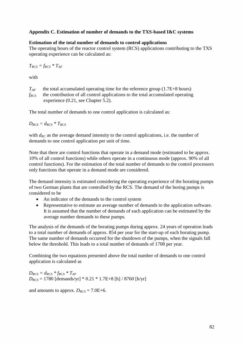
82

Appendix C. Estimation of number of demands to the TXS-based I&C systems

Estimation of the total number of demands to control applications

The operating hours of the reactor control system (RCS) applications contributing to the TXS

operating experience can be calculated as:

TRCS = fRCS * TAF

with

TAF the total accumulated operating time for the reference group (1.7E+8 hours)

fRCS the contribution of all control applications to the total accumulated operating

experience (0.21, see Chapter 5.2).

The total number of demands to one control application is calculated as:

DRCS = dRCS * TRCS

with dRC as the average demand intensity to the control applications, i.e. the number of

demands to one control application per unit of time.

Note that there are control functions that operate in a demand mode (estimated to be approx.

10% of all control functions) while others operate in a continuous mode (approx. 90% of all

control functions). For the estimation of the total number of demands to the control processors

only functions that operate in a demand mode are considered.

The demand intensity is estimated considering the operating experience of the borating pumps

of two German plants that are controlled by the RCS. The demand of the boring pumps is

considered to be

An indicator of the demands to the control system

Representative to estimate an average number of demands to the application software.

It is assumed that the number of demands of each application can be estimated by the

average number demands to these pumps.

The analysis of the demands of the borating pumps during approx. 24 years of operation leads

to a total number of demands of approx. 854 per year for the start-up of each borating pump.

The same number of demands occurred for the shutdown of the pumps, when the signals fall

below the threshold. This leads to a total number of demands of 1708 per year.

Combining the two equations presented above the total number of demands to one control

application is calculated as

DRCS = dRCS * fRCS * TAF

DRCS = 1780 [demands/yr] * 0.21 * 1.7E+8 [h] / 8760 [h/yr]

and amounts to approx. DRCS = 7.0E+6.

83

Estimation of the total number of demands to limitation applications

The total number of demands to the reactor limitation system (RLS) during the accumulated

operating experience is estimated in a similar manner as for the control system (see previous

chapter) as

TRLS = fRLS * TAF

with

fRLS the contribution of all limitation applications to the total accumulated operating experience

(0.12, see Chapter 5.2).

For the limitation system a representative and conservative demand rate of 1 demand/year per

application is considered. The total number of demands to the limitation system during the

accumulated operating experience of TXS is then calculated as:

DRLS = 1 [demand/yr] * 0.12 * 1.7E+8 [h] / 8760 [h/yr]

and amounts to approx. DRLS = 2390.

Estimation of the total number of demands to protection applications

The total number of demands to the reactor protection system (RPS) during the accumulated

operating experience is estimated in a similar manner as for the control system.

For the protection system a representative and conservative demand rate of 0.25 demands/year

per application is considered. This value is obtained by adding the frequencies of all initiating

events considered in the PSA to ensure the demand of all I&C functions in the different

accidents.

The total number of demands to the protection system during the accumulated operating

experience is calculated as:

DRPS = 0.25 [demand/yr] * 0.67 * 1.7E+8 [h] / 8760 [h/yr]

and amounts to 3360. Note that the contribution of the protection functions to the operating

experience is fRPS = 0.67 (see Chapter 5.2).

84

Appendix D. Example PSA model

In DIGREL, an existing simplified PSA model has been complemented with fault tree models

for a four-redundant distributed protection system in order to study and demonstrate the effect

of design features and modelling approaches. The example PSA-model represents a fictive

boiling water reactor (BWR), which has four-redundant safety systems. For details, see

(Authén et al. 2015).

Generally, same failure modes (types 1, 2a, 2b, 3, 4a and 4b) are considered in the model and

the same failure probabilities are used as suggested in this report. The fault trees for I&C has

been structured in hierarchical manner starting from the actuator down to measurements.

Details are described in (Authén et al. 2015). An example is given here to demonstrate the

appearance of software basic events.

Failure to start a safety critical pump is considered (e.g. emergency feedwater (EFW) pump).

The event is modelled according to the following fault tree (FT) structure. Software failure

basic events are shown as yellow boxes.

85

Failure of pump start signal (division x

considered)

DC power supply failure div. x *****

No signal from voting unit (VU) x

VUx processor failure (common to all VUx

outputs)

Detected VUx failures

Processor failure, detected

Subrack failure, detected

DC power supply failure div. x *****

Type 1 SW failure (common to all VU

outputs)

Type 2a SW failure (common to all VU

outputs)Type 3b SW failure

Undetected VUxfailures

Processor failure, undetected

No EFW start signal from VUx

Output module failure (specific to the EFWx

pump)

No EFW start signals from APUs (3-o-o-4

fails), division yconsidered below

Communication link failure (VUx–APUy)*

APUy failure

Undetected APUyfailures**

No EFW start signal from APUy

Type 4a SW failure “EFW start” AS

module in APU***

No inputs signals from divisions 1–4

Undetected failure of process measurement

(div. y) ****

Type 4b SW failure “EFW start” AS

module in VU

* Communication link failures (hardware failure and type 2b SW failure) are not critical for this function due to fail-safe actuation

** Detected failure of APU is not relevant in this example due to the fail-safe actuation

*** There may be more than one module involved depending on the actuation logic

**** Detected failure of measurement is not relevant in this example due to the fail-safe actuation

***** Fault trees for auxiliary power supply are not developed further here

86

Bibliographic Data Sheet NKS-341

Title Software reliability analysis for PSA: failure mode and data analysis

Author(s) Ola Bäckström1, Jan-Erik Holmberg2, Mariana Jockenhövel-

Barttfeld3, Markus Porthin4, Andre Taurines3, Tero Tyrväinen4

Affiliation(s) 1Lloyds Register AB, Sweden 2Risk Pilot AB, Sweden 3AREVA GmbH, Germany 4VTT Technical Research Centre of Finland Ltd

ISBN 978-87-7893-423-9

Date July 2015

Project NKS-R / DIGREL

No. of pages 85

No. of tables 10

No. of illustrations 19

No. of references 45

Abstract

max. 2000 characters

This report proposes a method for quantification of software

reliability for the purpose probabilistic safety assessment (PSA) for

nuclear power plants. It includes a failure modes taxonomy outlining

the relevant software failures to be modelled in PSA, quantification

models for each failure type as well as an analysis of operating data

on software failures concerning the TELEPERM® XS (TXS)

platform developed at AREVA.

Software related failure modes are defined by a) their location, i.e., in

which module the fault is, and b) their effect on the I&C unit. For a

processor the effect is either a fatal failure of the processor

(termination of the function and no outputs are produced) or non-

fatal failure where operation continues with possible wrong output

values. Following cases are relevant from the PSA modelling point

of view: 1) fatal failure causing loss of all subsystems that have the

same system software, 2a) fatal failure causing loss of one

subsystem, due to fault in system software, 2b) fatal failure in

communication modules of one subsystem. 3) fatal failure causing

failure of redundant set of I&C units in one subsystem, 4) non-fatal

failure associated with an application software module. In the case 4,

the failure effect can be a failure to actuate the function or a spurious

actuation.

87

The failure rates for software fault cases 1 and 2, associated with the

system software, are proposed to be estimated from general

operational data for same system software. The probabilities on

failure on demand for cases 3 and 4, associated with the application

software, are a priori assumed to correlate with the complexity and

degree of verification and validation (V&V) of the application. The

degree of V&V is related to the safety class of the software system

and the complexity can be assessed by analysing the logic diagram

specification of the application. A priori estimates could be updated

by operational data, which is demonstrated in the report.

Key words

PSA, Software reliability, Failure mode, Operational history data