NJ Cox's article on Stata
16
The Stata Journal (2002) 2, Number 3, pp. 314–329 Speaking Stata: On numbers and strings Nicholas J. Cox University of Durham, UK [email protected] Abstract. The great divide among data types in Stata is between numeric and string variables. Most of the time, which kind you want to use for particular variables is clear and unproblematic, but surprisingly often, users face difficulties in making the right decision or need to convert variables from one kind to another. The main problems that may arise and their possible solutions are surveyed with reference both to official Stata and to user-written programs. Keywords: pr0006, binary variables, categorical variables, Data Editor, dates, de- code, destring, encode, identifiers, missing values, numeric variables, spreadsheets, string functions, string variables, tostring, value labels 1 The great divide Stata datasets are composed of variables, and those variables may take one or more different types. What is more fundamental, however, is a division between two different kinds. Numeric variables may be byte, int, long, float, or double, depending on the number of bytes used for storage and whether values are held as integers or as real numbers with fractional parts, or more precisely, as the binary equivalents or approxi- mations to these. String variables hold character strings, those characters being broadly alphabetic (such as "a" or "A"), numeric (such as "3" or "7"), or other (chiefly various punctuation characters such as commas "," or (a very important example) spaces ""). As a small matter of history, Stata’s variable types were not all available from the beginning. Stata 1.0 was released in January 1985. Originally, variables could only be numeric, although value labels were possible. String variables were introduced in Stata 2.0 in June 1988, and they could hold any even number of characters from 2 (str2 type) to 80 (str80 type). Thus, a single character would need to be held in a str2 variable. Odd numbers of characters in string variables were soon allowed in Stata 2.1, which was released in September 1990. At the same time, the byte type was introduced to join the existing numeric types of int, long, float, and double. The next major change was not until February 2002, when Stata/SE, a between-releases “Special Edition”, raised the limit for string variables to 244 characters. Distinctions between different string types and different numeric types can be crucial, depending on the trade-off between holding all detail accurately enough and not using so much filespace or memory that operations become inordinately slow (or in extreme circumstances, even impossible). It is wasteful of memory, and, even if available memory is not limiting, it is wasteful in processing time to hold variables in types larger than is necessary. Conversely, the opposite pitfall should be clear: you can truncate or otherwise lose information with a variable type that is too small, or more generally, inappropriate. c 2002 Stata Corporation pr0006
Transcript of NJ Cox's article on Stata
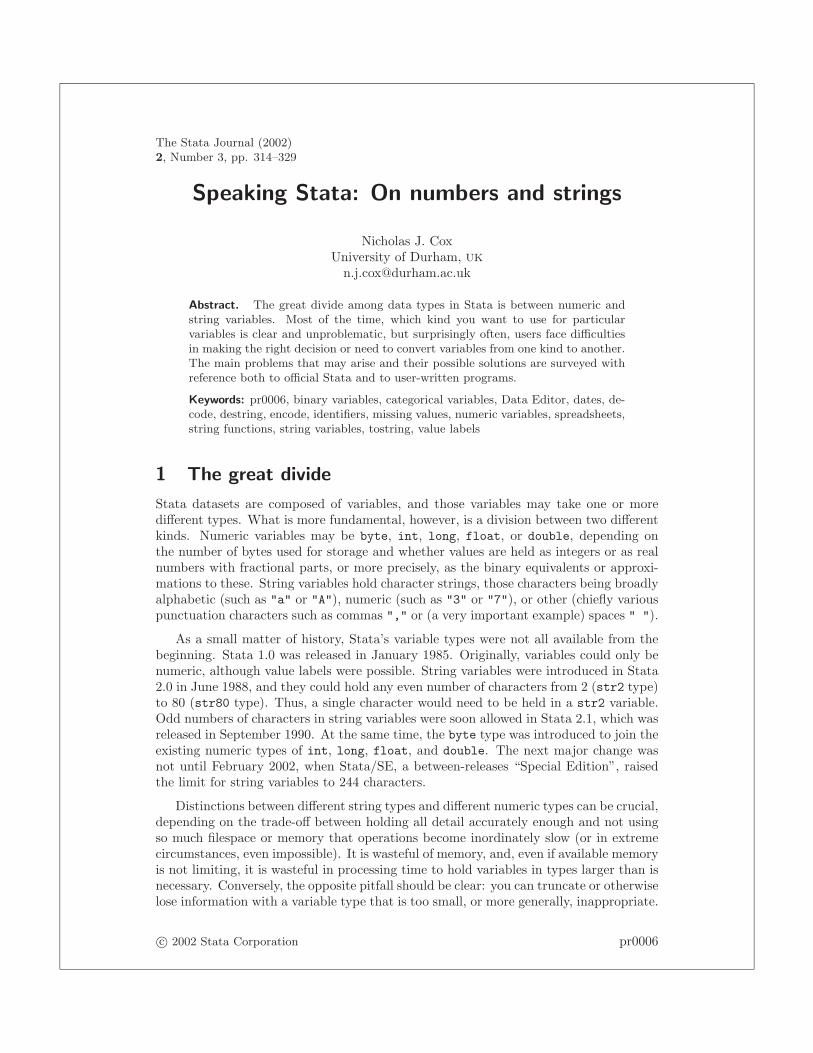
The Stata Journal (2002)2, Number 3, pp. 314–329
Speaking Stata: On numbers and strings
Nicholas J. CoxUniversity of Durham, UK
Abstract. The great divide among data types in Stata is between numeric andstring variables. Most of the time, which kind you want to use for particularvariables is clear and unproblematic, but surprisingly often, users face difficultiesin making the right decision or need to convert variables from one kind to another.The main problems that may arise and their possible solutions are surveyed withreference both to official Stata and to user-written programs.
Keywords: pr0006, binary variables, categorical variables, Data Editor, dates, de-code, destring, encode, identifiers, missing values, numeric variables, spreadsheets,string functions, string variables, tostring, value labels
1 The great divide
Stata datasets are composed of variables, and those variables may take one or moredifferent types. What is more fundamental, however, is a division between two differentkinds. Numeric variables may be byte, int, long, float, or double, depending onthe number of bytes used for storage and whether values are held as integers or as realnumbers with fractional parts, or more precisely, as the binary equivalents or approxi-mations to these. String variables hold character strings, those characters being broadlyalphabetic (such as "a" or "A"), numeric (such as "3" or "7"), or other (chiefly variouspunctuation characters such as commas "," or (a very important example) spaces " ").
As a small matter of history, Stata’s variable types were not all available from thebeginning. Stata 1.0 was released in January 1985. Originally, variables could only benumeric, although value labels were possible. String variables were introduced in Stata2.0 in June 1988, and they could hold any even number of characters from 2 (str2 type)to 80 (str80 type). Thus, a single character would need to be held in a str2 variable.Odd numbers of characters in string variables were soon allowed in Stata 2.1, which wasreleased in September 1990. At the same time, the byte type was introduced to join theexisting numeric types of int, long, float, and double. The next major change wasnot until February 2002, when Stata/SE, a between-releases “Special Edition”, raisedthe limit for string variables to 244 characters.
Distinctions between different string types and different numeric types can be crucial,depending on the trade-off between holding all detail accurately enough and not usingso much filespace or memory that operations become inordinately slow (or in extremecircumstances, even impossible). It is wasteful of memory, and, even if available memoryis not limiting, it is wasteful in processing time to hold variables in types larger than isnecessary. Conversely, the opposite pitfall should be clear: you can truncate or otherwiselose information with a variable type that is too small, or more generally, inappropriate.
c© 2002 Stata Corporation pr0006

N. J. Cox 315
You cannot fit a value such as "New York" in a str7 variable, and you cannot fit 3.14159in an int, as that dish is not right for holding that pie.
Three commands help in managing allocation of data types. For more information,see their manual entries in the Stata Reference Manuals; noting that replace is docu-mented in [R] generate. compress is an easy and safe way of reducing memory use. Itoften produces much smaller datasets, yet never loses information. replace is generallysmart in promoting variables whenever that is needed. A variable that starts out inlife as an int containing smallish integers will be changed to a float if calculationsin a replace introduce fractional parts. A string variable will be promoted wheneverit gets too long as the result of a replace, subject to the upper limit associated withyour executable (in Stata/SE 7.0, 244 characters and in Intercooled Stata 7.0 and SmallStata 7.0, 80 characters). recast is occasionally useful for upward promotions (anddangerously, when desired, demotions using its force option).
These commands provide ways of achieving changes of type, from one numeric typeto another or from one string type to another, but none allows change across the greatdivide, from numeric to string or vice versa. Crossing this divide is our main concernin this article. Not surprisingly, the main solutions occur in pairs, depending on thedirection of crossing, which helps to make sense of the variety of methods that exist.
Useful background for this article is given in various chapters of the Stata User’sGuide, especially [U] 15 Data, [U] 16 Functions and expressions, [U] 26 Com-mands for dealing with strings, and [U] 27 Commands for dealing with dates.
2 Numbers or strings?
2.1 Introduction
If you want to do numeric calculations in Stata with a variable, it should be numeric.Normally that would be your natural choice, and normally only by mistake will variablesthat should be numeric start out as string. (Such “mistakes” are more common thanyou might think, as you may already know; more will be said later, especially in Section5.) Despite its many uses for managing many kinds of datasets, even databases, Stata isprimarily statistical software, and so almost all users deal mostly with numeric variables.
However, the opposite rule—if you have information in the form of nonnumericcharacters, it should be held as string variables—does not always apply. Another wayto hold the nonnumeric information is as value labels linked to integer values of a numericvariable.
2.2 Choosing the right kind
What influences or determines the choice?

316 Speaking Stata
1. If the nonnumeric information you have defines categorical variables, especially ifthe number of categories is typically much fewer than the number of observations,it is best to use value labels. This is more efficient for storage and improvesuse of memory and processing time. In addition, some commands may not beapplied to string variables, even when that might appear sensible; for example,you cannot use graph on string variables to get something like a histogram. Incases like this, the error message is typically no observations, meaning preciselythat no numeric values are specified. To get such a graph, you need to produce theequivalent numeric variable with the nonnumeric values as value labels attachedto integers.
2. If anything, the case for doing this is even stronger with binary variables, which youmay also know as Boolean, dichotomous, dummy, indicator, logical, or quantal,depending on your upbringing. Whatever the name, they take on just two values,other than missing. As is well-known, a binary variable, especially one assignedvalues 0 and 1, may be used in many analyses: its mean has a direct and simpleinterpretation as a proportion, it may be used as a response variable in logitand probit models, and so on. All this, however, depends on a binary variablebeing held as numeric. (In passing, I commend the practice of naming a 0-1 binaryvariable for the category coded 1. If sex is 1 for female and 0 for male, then femaleis a better name. Which way round the coding is becomes more transparent.)
3. However, there are limits (in Stata/SE and Intercooled Stata 7.0, 65,536; in SmallStata 7.0, 1,000) on the number of value labels you may define that may beassociated with a variable. If you have more than 65,536 categories, you are morelikely to be dealing with individual identifiers than with classes of a categoricalvariable. An identifier is a name or a code that identifies people (places, businesses,whatever) uniquely, even if it is repeated in different observations, as in a paneldataset. But, whatever your situation, the limit in the version of Stata you areusing is an unbreakable law, and so beyond that limit, nonnumeric identifiers mustbe held as string variables.
4. Apart from the question of limits, unique identifiers will often conveniently beheld in string variables. There is little point in defining a value label if that valuelabel occurs only once. It is also less likely that you would want to use such avariable as defining one axis of a graph.
5. Less obviously, identifiers that consist entirely of numeric codes are often betterheld as string variables. U.S. Social Security Numbers (SSNs) are one of the mostfrequently discussed examples on Statalist. They consist of nine digits, commonlywritten as three fields separated by hyphens with the form aaa-gg-ssss; these fieldsare in turn the area number, the group number, and the serial number. Whenstored without hyphens, these SSNs can be read into Stata as numeric variables,but small problems often arise later. More generally, to hold multi-digit identifierswithout numeric precision problems (that is, holding every digit exactly) mayrequire the use of a long variable. To display such a variable (as with list)may require changing format to avoid most digits being lost whenever identifiers

N. J. Cox 317
are presented in scientific notation. (See [R] format.) For example, a floatnumeric variable set equal to 123456789 will by default be listed as 1.23e+08,shorthand for 1.23 × 10⁸. These are small and soluble problems, but they oftencause puzzlement to Stata users. Holding such identifiers as strings, even thoughevery character is numeric, solves those problems, with no apparent downside.
6. Similarly, categorical codes that are multi-digit numbers are often constructedhierarchically. That is, successive digits take you to finer detail within someclassification system with numerical codes (of diseases or occupations or products,say). When such codes are held as numbers, working from fine to coarse categories,or vice versa, can be done by tricks with int() or mod(). These tricks strikemany users as neat when they are familiar, but indirect or obscure when theyare not. The corresponding operations on such codes held as strings can be donewith substr() or index(), and these operations are often more transparent: thefirst three digits of a string variable code are specified by substr(code,1,3), forexample.
Stata 7.0 includes a special command, icd9, for dealing with ICD-9 or ICD-9-CM codes from the International Classification of Diseases, Ninth Revision or theInternational Classification of Diseases, Ninth Revision, Clinical Modification. See[R] icd9. In Stata, such codes must be held as string variables, because some codescontain nonnumeric characters; even if that were not true, it would be better tohold them as strings for ease of data processing.
7. Another important class of data is dates, especially daily dates, which come in avariety of formats. A date recorded as (say) "21 January 1952" or "1/21/1952"can be interpreted as numeric once there is some agreement on what is day 0:Stata’s convention is 1 January 1960, so 21 January 1952 is −2902. From thatrepresentation, we can easily find out, say, that 28 March 1952 was 67 days later,and so answer that and many more interesting or useful questions. However,variables with values like this can be read into Stata only as string variables: theycan be converted later to numeric dates, usually with the date() function. (Formore details, see [U] 27 Commands for dealing with dates.)
What might be called run-together dates with all digits numeric, say, 19520121or 1211952, can be read in either as numeric or as string. As already mentioned,a string representation has the advantage that precision and format problems areless likely, so long as the string type is large enough. For all that, you are mostlikely to want to convert dates in one of these representations to Stata dates. Suchconversion is at root a matter of separating the components of the run-togetherdates and then combining them once more using Stata functions for both. Atpresent, official Stata lacks facilities for handling run-together dates as such, buta user-written program may be accessed in an up-to-date Stata1 by typing sscdescribe todate.
1ssc was added to Stata 7.0 on 14 November 2001. If necessary, update your Stata(see McDowell 2001). If you do not have Stata 7.0, but you do have Internet access,http://www.stata.com/support/faqs/res/findit.html provides some explanation.

318 Speaking Stata
A run-together date such as 19520121 needs to be split into year, month, andday variables and then put together using the function mdy(). The splitting isat most three commands, which, if the date is held as string, all use the functionsubstr(). What todate does is wrap this all into one, using a pattern() optionto specify what the digits mean, so that
. todate date, gen(Date) pattern(yyyymmdd) format(%d)
performs the whole conversion to a Stata daily date variable. Half-years, quarters,months, and weeks are also supported, as are incompletely specified centuries andmultiple variables.
8. Evidently, any nonnumeric characters in dates, such as slashes or month names, aresufficient to imply that in the first instance the corresponding variables should beheld as string. More generally, any nonnumeric characters in otherwise numericfields are sufficient to make direct numeric representation impossible. So, forexample, a variable containing age intervals such as 0-9 or 10-19 must be held asstring or as numeric with value labels because of the included hyphens. That neednot stop approximate numeric equivalents from being computed, say, containingthe midpoint of each interval, or the endpoints being pried apart and put intoseparate and equivalent numeric variables.
9. If you are typing in the data, either by yourself or with assistance, it may be muchless labor to enter data as numeric. Value labels may be specified either beforeor later, and need only be typed once. (Sometimes, the associated value labelsmay already be defined, or the same value labels may be associated with severalvariables, as when a group of variables all record yes or no answers.) Saving ofeffort is greatest to the extent that small integers can be entered rather than longerstrings.
10. A quite different consideration arises sometimes, especially when teaching. Oneelementary error is to forget, particularly for statistical rather than data man-agement commands, that a variable may be numeric to Stata without being avariable which may fairly be included in a statistical model as is. It is arguablethat a habit of holding arbitrary numeric codes as strings provides some protectionagainst this blunder, helping you to avoid foolish statistics. In practice, however,this will rarely be a deciding issue.
2.3 Missing values
A reminder of what counts as missing with numeric and string variables may be helpfulhere.
Numeric missing in Stata is represented by a period ., which is always treated aslarger than any other numeric value. Thus, a sort of a numeric variable sorts missingvalues to the end of a dataset.
N. J. Cox 319
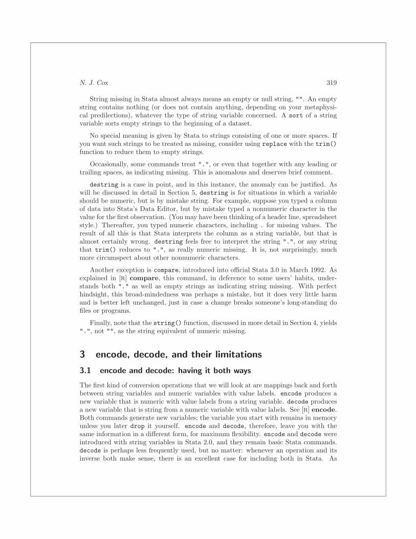
String missing in Stata almost always means an empty or null string, "". An emptystring contains nothing (or does not contain anything, depending on your metaphysi-cal predilections), whatever the type of string variable concerned. A sort of a stringvariable sorts empty strings to the beginning of a dataset.
No special meaning is given by Stata to strings consisting of one or more spaces. Ifyou want such strings to be treated as missing, consider using replace with the trim()function to reduce them to empty strings.
Occasionally, some commands treat ".", or even that together with any leading ortrailing spaces, as indicating missing. This is anomalous and deserves brief comment.
destring is a case in point, and in this instance, the anomaly can be justified. Aswill be discussed in detail in Section 5, destring is for situations in which a variableshould be numeric, but is by mistake string. For example, suppose you typed a columnof data into Stata’s Data Editor, but by mistake typed a nonnumeric character in thevalue for the first observation. (You may have been thinking of a header line, spreadsheetstyle.) Thereafter, you typed numeric characters, including . for missing values. Theresult of all this is that Stata interprets the column as a string variable, but that isalmost certainly wrong. destring feels free to interpret the string ".", or any stringthat trim() reduces to ".", as really numeric missing. It is, not surprisingly, muchmore circumspect about other nonnumeric characters.
Another exception is compare, introduced into official Stata 3.0 in March 1992. Asexplained in [R] compare, this command, in deference to some users’ habits, under-stands both "." as well as empty strings as indicating string missing. With perfecthindsight, this broad-mindedness was perhaps a mistake, but it does very little harmand is better left unchanged, just in case a change breaks someone’s long-standing dofiles or programs.
Finally, note that the string() function, discussed in more detail in Section 4, yields".", not "", as the string equivalent of numeric missing.
3 encode, decode, and their limitations
3.1 encode and decode: having it both ways
The first kind of conversion operations that we will look at are mappings back and forthbetween string variables and numeric variables with value labels. encode produces anew variable that is numeric with value labels from a string variable. decode producesa new variable that is string from a numeric variable with value labels. See [R] encode.Both commands generate new variables; the variable you start with remains in memoryunless you later drop it yourself. encode and decode, therefore, leave you with thesame information in a different form, for maximum flexibility. encode and decode wereintroduced with string variables in Stata 2.0, and they remain basic Stata commands.decode is perhaps less frequently used, but no matter: whenever an operation and itsinverse both make sense, there is an excellent case for including both in Stata. As

320 Speaking Stata
explained in [R] encode, decode can be very useful for match merging two datasets ona variable that has been encoded inconsistently.
Both commands work only on one variable at a time. Use of either on severalvariables might be accomplished best with the help of foreach, as explained in myprevious column (Cox 2002a). Suppose we want to encode variables a, b, c, d, and e.Here is a simple way of doing that, yielding Na, Nb, Nc, Nd, and Ne:
. foreach v in a b c d e {
. encode ‘v’, gen(N‘v’)
. }
3.2 Alphanumeric ordering and how to avoid it
One important detail is that by default, encode uses alphanumeric (i.e., ASCII) orderof string values to determine the order of integer codes. In the absence of any otherinformation, this is surely the best systematic way of carrying out the mapping. Thereare downstream consequences, however: the alphanumerically ordered value labels areusually uppermost in tables, on graphs, and in other output, and this order remainswired into the association between integers and value labels. It is often, indeed, theorder that you want. Grades "A" "B" "C" "D" "E" are mapped to 1 2 3 4 5 andtabulated in that order, which will often be fine (although also computing (6 − grade)might be useful for calculations). But, perhaps equally often, an alphanumeric order is anuisance, because it fails to respect some inherent meaning. String values "excellent","good", "fair", "poor", and "bad" belong in that sequence, and not sorted into "bad","excellent", "fair", and so forth.
The most general solution to the problem of arbitrary alphanumeric order is to writethe order you want into a set of value labels defined before the encode, and then tospecify that encode uses those mappings. Thus,
. label def opinion 1 "excellent" 2 "good" 3 "fair" 4 "poor" 5 "bad"
. encode answer, gen(opinion) label(opinion)
obliges Stata to ignore its default ordering and to follow the one you prefer.
Alphanumeric ordering may bite in a manner that is puzzling until you recall pre-cisely what such ordering means. Thus, age categories in ten-year intervals "0-9""10-19" . . . "90-99" will remain in this evidently natural order on alphanumeric or-dering. But split "0-9" into "0-4" and "5-9", and add "100-109", and you will findthat "5-9" will be sorted after "40-49" and that "100-109" will be sorted before"20-29". This is easy to explain. Although the ten numeric digits—in numeric order 0through 9—have the same alphanumeric order when represented as numeric characters"0" through "9", all strings when sorted are ordered as in a dictionary, so that ties arebroken on successive characters without any reference to their meaning. Once more,the best solution to avoid an unsatisfactory result from encode is to use a predefinedset of value labels codifying your desired order.
N. J. Cox 321
3.3 Start 1 encoding and how to avoid it
encode by default starts integer coding at 1. Sometimes you would prefer 0 as a start,especially for binary variables. One way to achieve this is by specifying the desired valuelabels ahead of the encode, as in the previous examples.
Retrospectively, fixing the values of a start 1 variable to start at 0 by subtracting 1is easy enough. The fiddly part is fixing the value labels to match. If you need to do thisa lot, two possible user-written tools are labedit (Gleason 1998, 1999) and labvalch(type ssc desc labutil).
Concretely, suppose you had a variable female coded as 1 and 2, and you decidethat this would be better coded as 0 and 1. You could just
. replace female = female - 1
or, if you are familiar with recode (see [R] recode), you might prefer
. recode female 1=0 2=1
but neither does anything to any value labels attached to female. If they also needfixing, the slow but sure way is just (supposing they have the same name as the variable)
. label define female 0 "male" 1 "female" 2 "" , modify
noting the detail of deleting the label for 2 by setting it to an empty string. The wayto do this with labvalch is
. labvalch female, from(1 2) to(0 1) delete(2)
which for just one variable is no gain. But for several sets of value labels, all to beshifted from start 1 to start 0, there could be a payoff:
. foreach lbl in female married employed retired yesno {
. labvalch ‘lbl’, from(1 2) to(0 1) delete(2)
. }
3.4 Ordering classes according to another variable
Defining a choice of labels by explicitly typing a label define before an encode is notideal for all situations. One common problem is that we want an ordering of classesaccording to their values on some other variable, so that a table or a graph will thenshow a more intelligible pattern, cutting free of the arbitrariness of the alphabet. SomeStata programs do this for you on the fly, but we still need to be able to do it forourselves whenever no such program exists for a particular task. This problem can arisefor any categorical variable, whether represented by a string variable or by a numericvariable with value labels.

322 Speaking Stata
Concretely, we might want categories ordered according to their associated frequency,or on the mean or maximum of some other variable. Again, we could compute theordering criterion directly and use the results to identify an appropriate set of valuelabels, which we then type out in a label define, but let us see if we can automatemost of that. In this kind of problem, the devices used most often vary from solutionsfrom first principles using by: (Cox 2002b) to canned egen functions (see [R] egen).(The fact that egen includes several functions applicable to string variables is oftenoverlooked.)
With the auto data, let us define the manufacturer name as the first word of make,and then count values by manufacturer:
. egen manuf = ends(make), head
. bysort manuf : gen freq = -_N
Note the minus sign. We are looking ahead, and foreseeing a sort, and, in particular,foreseeing that we will want highest values first, so that they will appear (say) as the firstrows of a table or the left-hand bars of a bar chart. That order is thus the opposite ofStata’s default sort order in which lowest values come first; negating values will reversethe order for us. (Naturally, if the default sort order is what you want, you should omitthe minus sign.)
Now we want to put the categories of manuf in the order defined by freq. Anotheregen function is very useful here.
. egen group = egroup(freq manuf), label(manuf)
egroup() produces the distinct categories defined by its arguments, in their (joint)sort order. The results are successive integers from 1 up, guaranteed (for example) toyield tidy graphs. egroup() here has two arguments. freq is mentioned first, becauseour main ordering is to be by frequency. manuf is mentioned next to ensure that anyties on freq are broken properly (for example, there are 7 Buicks and 7 Olds: 14 valuesthus have freq equal to 7, which must be split into those two groups).
egroup() is a user-written extension of official Stata’s egen, group(). (To access,type ssc desc egenmore.) The extension itself is just one extra wrinkle: the optionlabel may take an argument, lblvarlist, which specifies that we want the new variableto have value labels that are the values (or the value labels if they exist) of lblvarlist. Bycontrast, the label option of group(), which takes no argument, uses all the variablesin the varlist supplied to group() to construct value labels. With these data, we wouldhave labels like "-7 Buick", the -7 coming from the frequency, negated. Clearly, wewant only the manufacturer names in the labels.
(Continued on next page)

N. J. Cox 323
. tab group
group(manuf) Freq. Percent Cum.
Buick 7 9.46 9.46Olds 7 9.46 18.92
Chev. 6 8.11 27.03Merc. 6 8.11 35.14Pont. 6 8.11 43.24Plym. 5 6.76 50.00Datsun 4 5.41 55.41Dodge 4 5.41 60.81
VW 4 5.41 66.22AMC 3 4.05 70.27Cad. 3 4.05 74.32
Linc. 3 4.05 78.38Toyota 3 4.05 82.43
Audi 2 2.70 85.14Ford 2 2.70 87.84
Honda 2 2.70 90.54BMW 1 1.35 91.89Fiat 1 1.35 93.24
Mazda 1 1.35 94.59Peugeot 1 1.35 95.95Renault 1 1.35 97.30Subaru 1 1.35 98.65Volvo 1 1.35 100.00
Total 74 100.00
There are two (and perhaps a half) basic steps here, but the method is quite general.First, generate the variable on which you want to order classes as a group statistic.Remember negation if you want to reverse the order. Second, use egen, egroup()label() to produce the groups in the right order and with the right labels. These stepsproduce a variable that may then be used for tables, graphs, etc.
4 real() and string(): the brute force solutions
There are brute force methods of crossing the divide. The function real() extractsthe numeric content of a string expression, such as a string variable. The functionstring() converts a numeric expression, such as a numeric variable, to a string. Thedocumentation for some software talks of coercion from one type to another. Althoughthat is not a common term in discussing Stata functions, it captures well the flavor ofwhat is discussed in this section.
Given any doubt, real() yields numeric missing. Therefore, watching carefully formessages about missing values is always worthwhile. Having a look at the problemobservations may reveal some problems with easy fixes, or at least a variable bettertackled with destring (see Section 5). For example, real("1,234") yields numericmissing. The intelligence that strips the comma is not built in to the function. Moregenerally, given string variable strvar, which contains mostly numeric information, theseinspections should pinpoint what cannot be interpreted as numeric:

324 Speaking Stata
. tabulate strvar if real( strvar) == .
. list strvar if real( strvar) == .
The brute force may seem to lie on one side. Although not all characters are numeric,surely all numeric characters are characters. Nevertheless, the companion functionstring() is also fairly described as a brute force solution, for the same fundamentalreason: without some forethought, it is possible to miss information in your data. Nine-digit identifiers such as U.S. Social Security Numbers provide a simple but forcefulexample. string(123456789) yields "1.23e+08", meaning 1.23 × 10⁸. The key detailneeded is that string() is really a function taking two arguments, the second of which isa numeric or date or time format. string(123456789, "%12.0g") yields "123456789"in the way that you would expect. The point is simply that the default format is not,and cannot be, ideal for all circumstances.
For simple cases, real() and string() may perform perfectly well, but beware theirbrutality when data are more complicated than you realized.
5 destring and tostring: correcting mistaken choices
5.1 Learning from history
As we have seen, the main solutions to problems with the great divide occur in pairs, apair for each operation and its inverse. The last pair we will look at is the official Statacommand destring and its sibling, the user-written command tostring. destring hasthe longer history. After publication and revision in the Stata Technical Bulletin (STB)(Cox and Gould 1997; Cox 1999a, 1999b), it was adopted in official Stata in version 7.tostring came later (Cox and Wernow 2000a, 2000b).
The history of destring has no practical implications, except for any users whostarted with the STB version and became accustomed to the ways in which it worked,but it raises major issues to do with command design. When destring was incorporatedin official Stata, it was largely rewritten to produce a more focused command. Whywas that?
First, the original destring command violated Stata’s philosophy in that it was tooeasy to change much of your dataset without the safeguard of having to spell out someinjunction such as “, replace”. destring now not only insists on that, it also obligesyou to specify force whenever the creation of a numeric variable would lose informationcontained in the original string variable.
More specifically, destring allowed a variable to be replaced by an encoded equiva-lent, unless users specifically opted out of that. Positively, it offered the power to solveseveral dataset problems with no more than a single destring (no variable list, nooptions). Existing numeric variables would be unchanged, string variables with purelynumeric content would be replaced by their numeric equivalents, and other string vari-ables would be encoded if possible. But, by the same token, this made it too easy tomisunderstand what had been done, with all sorts of further consequences. If x were

N. J. Cox 325
string with numeric content, then summarize x is a perfectly reasonable thing to typeafter destring. If x were string with no numeric content, and as such was encoded,then summarize x is all too likely to be wrong or meaningless. If the price of liberty iseternal vigilance, then in the case of the original destring, it was bought too dearly.
What underlies all this is a general principle: it is best when Stata commands do onething well. In retrospect, it was a bad idea to let destring overlap in functionality withencode. On adoption in Stata 7.0, therefore, it was decided to sharpen the distinctionbetween them. encode is designed for situations in which you have a string variablecontaining nonnumeric text (e.g., "male", "female"), and wish to have the equivalentinformation as a numeric variable with labels. destring is designed for situations inwhich you have a string variable containing numeric text (e.g., "1", "2"), which youwish to convert to the numeric variable that it should properly be. Usually, that variableis now string because of some mistake. How could such a mistake be made?
5.2 Mistaken string variables
Stata’s Data Editor
One way in which a mistake can arise is when entering data into Stata’s Data Editor (see[R] edit). Some users, especially if new to Stata and accustomed to the license providedby spreadsheets, may type header information, say, a column title or explanatory text,into the top rows of the editor. To Stata, however, these rows define the first few valuesof its variables; its rule is that all cells in any given column must be of the same variabletype.
Just the first observation can be crucial in interacting with the Data Editor, whichattempts to be as smart as possible and to divine your intentions from what you type.Enter any nonnumeric text in the first cell of a column, and the editor instantly thinks,“Aha! This user wants this variable to be a string variable”, and it promptly andsilently creates that variable as string. Even if all cells below are entered with numerictext, this causes edit no puzzlement, as numeric characters are perfectly acceptable ina string variable. The editor will silently promote a string variable to a wider type iflater values require that. However, the editor will never unilaterally change a variableof yours from string to numeric, or from numeric to string, and the same holds for allother Stata commands. To do that would entail guessing at what you really intend,with the possibility of making an incorrect guess and making a mess of your dataset.To do that could seriously compromise the integrity of your data.
This is a strong principle, which can admit no exceptions, even though the conse-quences may be irritating. Suppose, for example, that the mistake lay only in a first rowof text values across a dataset, defining the first observation. Realizing your mistake,you simply delete the first row. Now, perhaps most—or even all—of the columns in theeditor contain purely numeric text, for the simple reason that they were all intendedto contain numeric variables. Should the editor change its mind, and change thesevariables unilaterally to numeric? No. For all the editor knows, you really wanted the
326 Speaking Stata
numeric text to be a string variable. After all, Section 2 gave several good reasons forstoring numeric text in a string variable. More generally, Stata should not be in thebusiness of making guesses about your data, or of assuming that it knows better thanyou do precisely what you intend your data to be. It follows that you must specify yourintentions explicitly, using destring.
Naturally, edit’s principle that first impressions count is not the only basis on whichit could have been designed. However, a data editor in which you were obliged to specifya variable type before a variable was entered would not have the friendliness and freedomof action that one might fairly expect.
Spreadsheets and other software
The same kind of issue can arise when importing data from spreadsheets, from otherapplication programs (say, under Windows, by way of the clipboard), or from ASCII
files created by these programs, by text editors, or by word processors. Spreadsheetsprovide good examples of some of the possible difficulties that lead to mistaken stringvariables. The same or similar problems can also occur with other programs or theircreations, which might be read in with a command like insheet. (See [R] insheet.)
Some of these problems depend on which software you are using. A list of variouspitfalls that have been reported thus far may, with good fortune, include some that willnever open up before you.
1. A single cell in a column containing a nonnumeric character, such as a letter, isenough for Stata to treat that column as a string variable. As implemented inStata 7.0, destring includes an option for stripping commas, dollar signs, percentsigns, and other nonnumeric characters. It also allows automatic conversion ofpercent data.
2. What appear to be purely numeric data in a spreadsheet are often treated by Stataas string variables because they include spaces. You, or whoever created your datafile, may inadvertently enter space characters in cells that are otherwise empty.Although a spreadsheet may strip leading and trailing spaces from numeric entries,it will not trim spaces from character entries. One or more space characters bythemselves constitute a valid character entry and are stored as such. Stata maydutifully read the entire column as a string variable. If so, you could delete suchstray spaces in the spreadsheet, or you can use a text editor or scripting languageon an exported text file, or again you could use destring.
3. Much formatting within a spreadsheet interferes with Stata’s ability to interpretthe data reasonably. Just before saving the data as a text file, make sure allformatting is turned off, at least temporarily.
4. With integer-like codes such as ICD-9 codes or U.S. Social Security Numbers thatdo not contain a dash, leading zeros will get dropped when you paste into Stata.One solution is to flag within the first line that the variable is string: add a
N. J. Cox 327
nonnumeric character in your spreadsheet on that line, and then remove it inStata. Alternatively, the missing leading zeros can be replaced in Stata in aconversion to string:
. gen str12 strvar = string( numvar,"%012.0f")
The second argument on the right-hand side of this command is a format specifyingdisplay of leading zeros in conversion of numvar to its string equivalent. See[R] format.
5.3 Mistaken numeric variables
destring has a sibling, tostring, for the less common situation in which you decidethat the information held in numeric variables really should be held in string form. Asdiscussed in Section 2, this need arises most commonly when the numeric variable isreally an identifier of some kind, or a complicated categorical code, and you wish tocarry out string manipulations using Stata’s string functions.
tostring is essentially a convenience command, with various features, includingautomatic determination of which string type is needed; a default format (%12.0g)better suited to integers, whether held as byte, int or long; and the ability to workwith several variables at once. Conversely, some features are, in retrospect, bad, or atleast arguable, choices, and will be withdrawn in future versions: being able to decode;being able to overwrite existing variables without specifying “, replace”; and beingable to ignore details (especially in fractional parts) without specifying a force option.
6 Statistically defined variable types?
It will be clear by now that the distinctions between Stata’s variable types are basedmainly on computing distinctions, rather than any statistical or other distinctions basedon the scales of measurement used, the roles played by variables in statistical models, orsimilar considerations. In particular, categorical variables may be held in quite differentways within Stata. Stata does show a marked preference that they be held in numericvariables with value labels attached, insofar as that allows the widest possible range ofcommands to be used, but for some purposes, it is also a good idea to hold the sameinformation in string form.
Concretely, Stata has (for example) no exact equivalent to the ideas of factors orto ordered factors available in S, S-Plus, or R (see, for example, Chambers and Hastie1992). What may seem at first an exception to this assertion, the category() andcontinuous() options of anova (explained in [R] anova), is in fact a demonstration ofit; that is, anova requires a specification of how it is to treat variables. It has no wayof knowing from the information stored by Stata how variables are to be interpreted.Also, this specification is purely for the moment, and has no consequences for any futurecommands, except those that process output from the model just fitted. On occasion,when the best way to treat some variable (say age) is in doubt, anova commands could
328 Speaking Stata
even treat a variable as in turn categorical and continuous, in a bid to identify the betterrepresentation. What Stata gains and what it loses from this way of treating variablesmakes a topic for interesting future discussions.
7 Summary
The variety of routes that cross the great divide between numeric types and stringtypes in Stata may be reduced to intelligible order, despite some mistaken ventures bypioneers. Use decode or encode to generate new variables of different kinds holdingthe same information. Use real() and string() for conversions or coercions, checkingeach time on whatever cannot be coerced to different kind, and is thus assigned missing.Use destring or tostring to correct mistakes whenever you have variables of one kindthat really should be of the other kind.
8 What’s next?
In the next column, we will look at the confusing territory stretching from built-infunctions to egen functions. In engineering terms, the range is from ‘black boxes’ (youcannot look inside) to ‘white boxes’ (you can look inside and borrow ideas). Even withthe large and growing number of functions that they provide, there will always be gaps,so the key question of how best to fill those gaps for yourself will also be discussed.
9 Acknowledgments
Some of the work reported here benefited greatly from the collaboration and commentsof William Gould, Jeremy Wernow, and Vince Wiggins. Material on spreadsheets isbased partly on an FAQ to which contributions were made by Ted Anagnoson, DanChandler, Ronan Conroy, James Hardin, David Moore, Paul Wicks, and Eric Wruck.
10 ReferencesChambers, J. M. and T. J. Hastie. 1992. Statistical Models in S. Pacific Grove, CA:
Wadsworth and Brooks/Cole.
Cox, N. J. 1999a. dm45.1: Changing string variables to numeric: update. Stata Tech-nical Bulletin 49: 2. In Stata Technical Bulletin Reprints, vol. 9, 14. College Station,TX: Stata Press.
—. 1999b. dm45.2: Changing string variables to numeric: update. Stata TechnicalBulletin 52: 2. In Stata Technical Bulletin Reprints, vol. 9, 14. College Station, TX:Stata Press.
—. 2002a. Speaking Stata: How to face lists with fortitude. Stata Journal 2(2): 202–222.

N. J. Cox 329
—. 2002b. Speaking Stata: How to move step by: step. Stata Journal 2(1): 86–102.
Cox, N. J. and W. W. Gould. 1997. dm45: Changing string variables to numeric. StataTechnical Bulletin 37: 4–6. In Stata Technical Bulletin Reprints, vol. 7, 34–37. CollegeStation, TX: Stata Press.
Cox, N. J. and J. B. Wernow. 2000a. dm80: Changing numeric variables to string.Stata Technical Bulletin 56: 8–12. In Stata Technical Bulletin Reprints, vol. 10,24–28. College Station, TX: Stata Press.
—. 2000b. dm80.1: Update to changing numeric variables to string. Stata TechnicalBulletin 57: 2. In Stata Technical Bulletin Reprints, vol. 10, 28–29. College Station,TX: Stata Press.
Gleason, J. R. 1998. dm56: A labels editor for Windows and Macintosh. Stata TechnicalBulletin 43: 3–6. In Stata Technical Bulletin Reprints, vol. 8, 5–10. College Station,TX: Stata Press.
—. 1999. dm56.1: Update to labedit. Stata Technical Bulletin 51: 2. In Stata TechnicalBulletin Reprints, vol. 9, 15. College Station, TX: Stata Press.
McDowell, A. 2001. From the help desk. Stata Journal 1(1): 76–85.
About the Author
Nicholas Cox is a statistically-minded geographer at the University of Durham. He contributestalks, postings, FAQs, and programs to the Stata user community. He has also co-authoredeight commands in official Stata. He was an author of several inserts in the Stata TechnicalBulletin and is Executive Editor of The Stata Journal.