
NIST Weather Station for Photovoltaic and Building System ... · This effort was conducted by the...
55
NIST Technical Note 1913 NIST Weather Station for Photovoltaic and Building System Research Matthew T. Boyd This publication is available free of charge from: http://dx.doi.org/10.6028/NIST.TN.1913
-
Upload
truongphuc -
Category
Documents
-
view
216 -
download
0
Transcript of NIST Weather Station for Photovoltaic and Building System ... · This effort was conducted by the...
NIST Technical Note 1913
NIST Weather Station for
Photovoltaic and Building System
Research
Matthew T. Boyd
This publication is available free of charge from: http://dx.doi.org/10.6028/NIST.TN.1913


NIST Technical Note 1913
NIST Weather Station for
Photovoltaic and Building System
Research
Matthew T. Boyd
Energy and Environment Division
Engineering Laboratory
This publication is available free of charge from:
http://dx.doi.org/10.6028/NIST.TN.1913
March 2016
U.S. Department of Commerce Penny Pritzker, Secretary
National Institute of Standards and Technology
Willie May, Under Secretary of Commerce for Standards and Technology and Director

Certain commercial entities, equipment, or materials may be identified in this
document in order to describe an experimental procedure or concept adequately.
Such identification is not intended to imply recommendation or endorsement by the
National Institute of Standards and Technology, nor is it intended to imply that the
entities, materials, or equipment are necessarily the best available for the purpose.
National Institute of Standards and Technology Technical Note 1913
Natl. Inst. Stand. Technol. Tech. Note 1913, 43 pages (March 2016)
CODEN: NTNOEF
This publication is available free of charge from:
http://dx.doi.org/10.6028/NIST.TN.1913

ii
Preface
This effort was conducted by the Energy and Environment Division in the Engineering Laboratory at the National
Institute of Standards and Technology (NIST). This document describes the meteorological instruments and data
acquisition system (DAS) at a research-grade weather station on the NIST campus in Gaithersburg, Maryland, USA,
including the rationale for the selected instruments, data loggers, control software, and supplementary devices. The
intended audiences are researchers who wish to use the gathered data, including the compiled weather files, for
analysis and modeling of photovoltaic (PV) systems, building energy, or meteorological values, as well as designers
who are interested in building a similar research-grade weather station. Modelers and analysts who are interested in
using the data in collaboration on new research before a public data portal is available can contact the author.
Author Information
Matthew T. Boyd
Mechanical Engineer
National Institute of Standards and Technology
Engineering Laboratory
100 Bureau Drive, Mailstop 8632
Gaithersburg, MD 20899-8632
Tel.: 301-975-6444
Email: [email protected]
iii
Abstract
A weather station has been constructed on the Gaithersburg, Maryland campus of the National Institute of Standards
and Technology (NIST) as part of a research effort to assess performance of photovoltaic and building systems. This
weather station includes research-grade instrumentation to measure all standard meteorological quantities plus
various additional solar irradiance spectral bands, full spectrum curves, and directional components using multiple
irradiance sensor technologies. Reference photovoltaic (PV) modules are also monitored on site to provide
comprehensive baseline measurements for the PV arrays on campus. Images of the whole sky are captured, along
with images of the instrumentation and reference modules to document any obstructions or anomalies. Nearly all
measurements are sampled and saved every 1 second, with monitoring having started August 1, 2014. This report
describes the instrumentation approach to measure the meteorological and photovoltaic quantities and acquire the
images for use in computer model validation or weather monitoring.
Keywords
meteorology, weather station, data acquisition, solar, photovoltaic

iv
Table of Contents
Preface .......................................................................................................................................................................... ii
Abstract........................................................................................................................................................................ iii
Table of Contents..........................................................................................................................................................iv
List of Figures ............................................................................................................................................................. vii
List of Tables ............................................................................................................................................................. viii
Glossary ........................................................................................................................................................................ix
1. Introduction ............................................................................................................................................................... 1
2. Overview ................................................................................................................................................................... 3
2.1. Summary ............................................................................................................................................................. 3
2.1.1. Facilities....................................................................................................................................................... 4
2.1.2. Shading ........................................................................................................................................................ 5
3. Measurements ............................................................................................................................................................ 6
3.1. Summary ............................................................................................................................................................. 6
3.2. Global Shortwave Irradiance .............................................................................................................................. 8
3.2.1. Sensors ......................................................................................................................................................... 8
3.2.2. Calibrations .................................................................................................................................................. 8
3.2.3. Locations and Orientations .......................................................................................................................... 8
3.2.4. Mounting and Alignment ............................................................................................................................. 9
3.2.5. Wiring ........................................................................................................................................................ 10
3.3. Direct and Diffuse Shortwave Irradiance.......................................................................................................... 10
3.3.1. Sensors ....................................................................................................................................................... 10
3.3.2. Calibrations ................................................................................................................................................ 10
3.3.3. Locations and Orientations ........................................................................................................................ 10
3.3.4. Mounting and Alignment ........................................................................................................................... 11
3.4. Longwave Irradiance ........................................................................................................................................ 11
3.5. UV Irradiance ................................................................................................................................................... 12
3.6. Spectral Irradiance ............................................................................................................................................ 12
3.7. Ambient Temperature ....................................................................................................................................... 12
3.7.1. Sensors ....................................................................................................................................................... 12
3.7.2. Calibrations ................................................................................................................................................ 13
3.7.3. Locations and Orientations ........................................................................................................................ 13
3.7.4. Wiring ........................................................................................................................................................ 14
3.8. Wind ................................................................................................................................................................. 14
v
3.8.1. Sensors ....................................................................................................................................................... 14
3.8.2. Calibrations ................................................................................................................................................ 15
3.8.3. Locations and Orientation .......................................................................................................................... 15
3.8.4. Mounting and Alignment ........................................................................................................................... 15
3.8.5. Wiring ........................................................................................................................................................ 15
3.9. Ambient Pressure and Humidity ....................................................................................................................... 15
3.10. Precipitation .................................................................................................................................................... 16
3.10.1. Liquid....................................................................................................................................................... 16
3.10.2. Solid ......................................................................................................................................................... 16
3.11. Reference Modules ......................................................................................................................................... 17
3.12. Module Temperature ...................................................................................................................................... 19
3.12.1. Sensors ..................................................................................................................................................... 19
3.12.2. Calibrations .............................................................................................................................................. 20
3.12.3. Locations ................................................................................................................................................. 20
3.12.4. Mounting and Alignment ......................................................................................................................... 21
3.12.5. Wiring ...................................................................................................................................................... 21
4. Data Acquisition and Control .................................................................................................................................. 21
4.1. Data loggers ...................................................................................................................................................... 21
4.1.1. Components ............................................................................................................................................... 21
4.1.2. Locations and Housing .............................................................................................................................. 23
4.1.3. Wiring ........................................................................................................................................................ 24
4.1.4. Configuration ............................................................................................................................................. 25
4.1.5. Sampling Rates and Parallel Processing .................................................................................................... 25
4.1.6. Time Synchronization ................................................................................................................................ 25
4.1.7. Channel Ranges ......................................................................................................................................... 25
4.1.8. Self-Calibration.......................................................................................................................................... 25
4.1.9. Measurement Techniques .......................................................................................................................... 25
4.1.10. Control ..................................................................................................................................................... 27
4.1.11. Data storage and processing .................................................................................................................... 28
4.2. Spectroradiometers ........................................................................................................................................... 28
4.3. Reference Modules ........................................................................................................................................... 28
4.4. Cameras ............................................................................................................................................................ 29
4.4.1. Module and Instrument .............................................................................................................................. 29
4.4.2. All Sky ....................................................................................................................................................... 30
5. Backup Power .......................................................................................................................................................... 32
vi
5.1. Data loggers ...................................................................................................................................................... 32
5.2. Central UPS ...................................................................................................................................................... 32
5.3. Distributed UPSs .............................................................................................................................................. 32
6. Data Archiving and Monitoring ............................................................................................................................... 33
7. Uncertainty .............................................................................................................................................................. 34
8. Maintenance ............................................................................................................................................................ 34
Acknowledgements ..................................................................................................................................................... 34
References ................................................................................................................................................................... 34
Appendix A. The Saved Data Values From Each Data Logger .................................................................................... 1
Appendix B. Module Data Sheets ................................................................................................................................ 1
vii
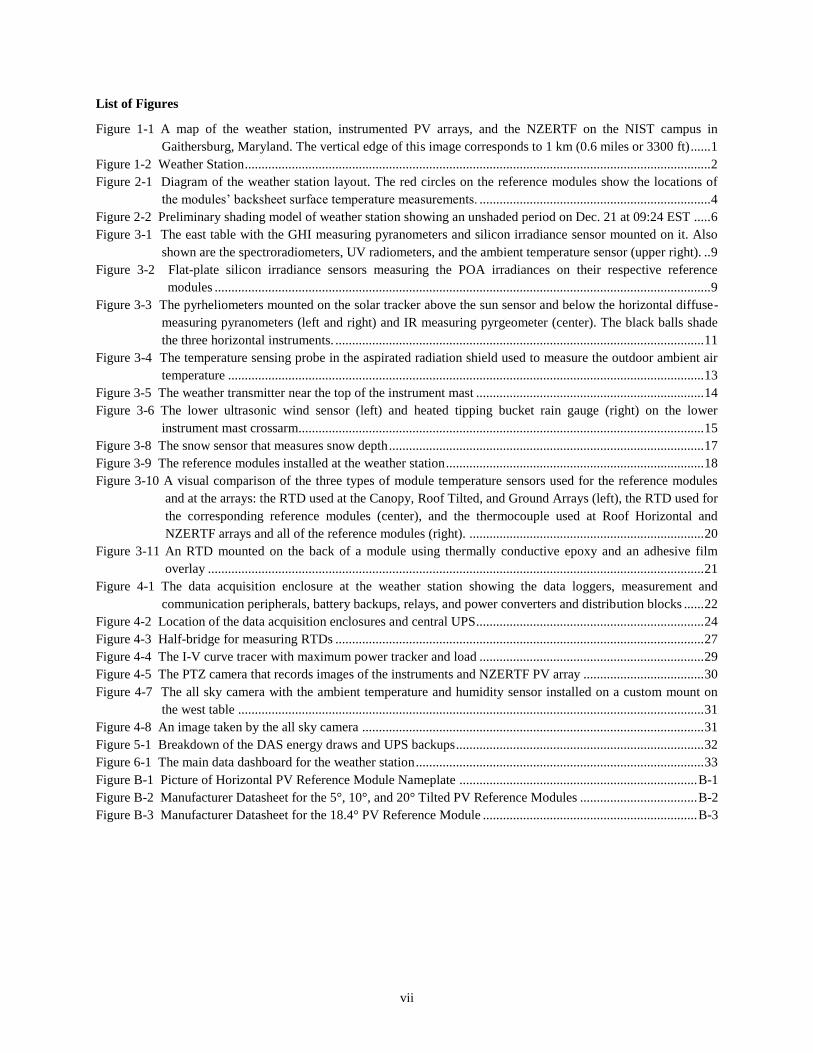
List of Figures
Figure 1-1 A map of the weather station, instrumented PV arrays, and the NZERTF on the NIST campus in
Gaithersburg, Maryland. The vertical edge of this image corresponds to 1 km (0.6 miles or 3300 ft) ...... 1 Figure 1-2 Weather Station ........................................................................................................................................... 2 Figure 2-1 Diagram of the weather station layout. The red circles on the reference modules show the locations of
the modules’ backsheet surface temperature measurements. ..................................................................... 4 Figure 2-2 Preliminary shading model of weather station showing an unshaded period on Dec. 21 at 09:24 EST ..... 6 Figure 3-1 The east table with the GHI measuring pyranometers and silicon irradiance sensor mounted on it. Also
shown are the spectroradiometers, UV radiometers, and the ambient temperature sensor (upper right). .. 9 Figure 3-2 Flat-plate silicon irradiance sensors measuring the POA irradiances on their respective reference
modules .................................................................................................................................................... 9 Figure 3-3 The pyrheliometers mounted on the solar tracker above the sun sensor and below the horizontal diffuse-
measuring pyranometers (left and right) and IR measuring pyrgeometer (center). The black balls shade
the three horizontal instruments. .............................................................................................................. 11 Figure 3-4 The temperature sensing probe in the aspirated radiation shield used to measure the outdoor ambient air
temperature .............................................................................................................................................. 13 Figure 3-5 The weather transmitter near the top of the instrument mast .................................................................... 14 Figure 3-6 The lower ultrasonic wind sensor (left) and heated tipping bucket rain gauge (right) on the lower
instrument mast crossarm......................................................................................................................... 15 Figure 3-8 The snow sensor that measures snow depth .............................................................................................. 17 Figure 3-9 The reference modules installed at the weather station ............................................................................. 18 Figure 3-10 A visual comparison of the three types of module temperature sensors used for the reference modules
and at the arrays: the RTD used at the Canopy, Roof Tilted, and Ground Arrays (left), the RTD used for
the corresponding reference modules (center), and the thermocouple used at Roof Horizontal and
NZERTF arrays and all of the reference modules (right). ...................................................................... 20 Figure 3-11 An RTD mounted on the back of a module using thermally conductive epoxy and an adhesive film
overlay .................................................................................................................................................... 21 Figure 4-1 The data acquisition enclosure at the weather station showing the data loggers, measurement and
communication peripherals, battery backups, relays, and power converters and distribution blocks ...... 22 Figure 4-2 Location of the data acquisition enclosures and central UPS .................................................................... 24 Figure 4-3 Half-bridge for measuring RTDs .............................................................................................................. 27 Figure 4-4 The I-V curve tracer with maximum power tracker and load ................................................................... 29 Figure 4-5 The PTZ camera that records images of the instruments and NZERTF PV array .................................... 30 Figure 4-7 The all sky camera with the ambient temperature and humidity sensor installed on a custom mount on
the west table ........................................................................................................................................... 31 Figure 4-8 An image taken by the all sky camera ...................................................................................................... 31 Figure 5-1 Breakdown of the DAS energy draws and UPS backups .......................................................................... 32 Figure 6-1 The main data dashboard for the weather station ...................................................................................... 33 Figure B-1 Picture of Horizontal PV Reference Module Nameplate ....................................................................... B-1
Figure B-2 Manufacturer Datasheet for the 5°, 10°, and 20° Tilted PV Reference Modules ................................... B-2
Figure B-3 Manufacturer Datasheet for the 18.4° PV Reference Module ................................................................ B-3

viii
List of Tables
Table 2-1 Location of the Weather Station ................................................................................................................... 3 Table 3-1 Summary of the Measurements and Respective Instruments Installed at the Weather Station .................... 6 Table 3-2 Summary of Reference Modules ................................................................................................................ 18 Table A-1 The Saved Data Values From Each Data Logger .................................................................................... A-1
ix
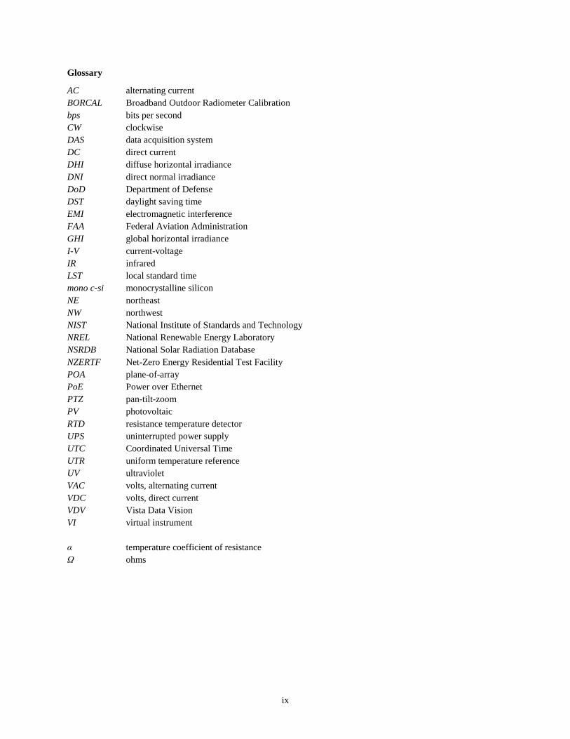
Glossary
AC alternating current
BORCAL Broadband Outdoor Radiometer Calibration
bps bits per second
CW clockwise
DAS data acquisition system
DC direct current
DHI diffuse horizontal irradiance
DNI direct normal irradiance
DoD Department of Defense
DST daylight saving time
EMI electromagnetic interference
FAA Federal Aviation Administration
GHI global horizontal irradiance
I-V current-voltage
IR infrared
LST local standard time
mono c-si monocrystalline silicon
NE northeast
NW northwest
NIST National Institute of Standards and Technology
NREL National Renewable Energy Laboratory
NSRDB National Solar Radiation Database
NZERTF Net-Zero Energy Residential Test Facility
POA plane-of-array
PoE Power over Ethernet
PTZ pan-tilt-zoom
PV photovoltaic
RTD resistance temperature detector
UPS uninterrupted power supply
UTC Coordinated Universal Time
UTR uniform temperature reference
UV ultraviolet
VAC volts, alternating current
VDC volts, direct current
VDV Vista Data Vision
VI virtual instrument
α temperature coefficient of resistance
Ω ohms
1
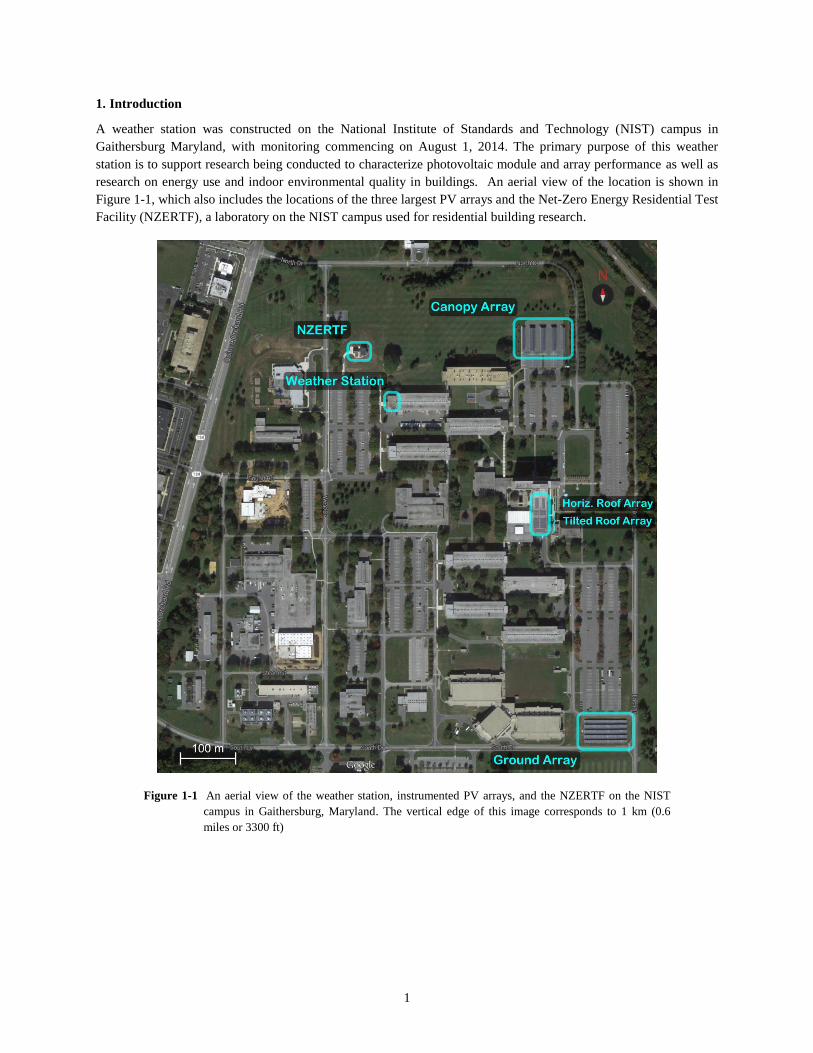
1. Introduction
A weather station was constructed on the National Institute of Standards and Technology (NIST) campus in
Gaithersburg Maryland, with monitoring commencing on August 1, 2014. The primary purpose of this weather
station is to support research being conducted to characterize photovoltaic module and array performance as well as
research on energy use and indoor environmental quality in buildings. An aerial view of the location is shown in
Figure 1-1, which also includes the locations of the three largest PV arrays and the Net-Zero Energy Residential Test
Facility (NZERTF), a laboratory on the NIST campus used for residential building research.
Figure 1-1 An aerial view of the weather station, instrumented PV arrays, and the NZERTF on the NIST
campus in Gaithersburg, Maryland. The vertical edge of this image corresponds to 1 km (0.6
miles or 3300 ft)

2
Research-grade (i.e., low uncertainty) sensors are installed, as shown in Figure 1-2, to measure various
meteorological quantities, including:
direct normal irradiance (DNI)
diffuse horizontal irradiance (DHI)
global horizontal irradiance (GHI)
infrared (IR) irradiance (net and total)
ultraviolet (UV) irradiance (A, B, and total)
spectral irradiance curves
snow depth
wind speed and direction
humidity
precipitation
barometric pressure
hail count
ambient temperature
Figure 1-2 Weather Station
The data acquisition system (DAS) saves measurement values every 1 second along with the status of the solar
tracker and other components. A current-voltage (I-V) tracer with a maximum power tracker and load saves curve
traces from reference modules installed in the orientations of the modules in each of the PV arrays on campus every
1 minute, along with one-minute averaged maximum power measurements from one-second samples. Cameras were
also installed that capture images of the entire sky every 8 seconds and close-up images of the instrumentation,
reference modules, and NZERTF PV array every 5 minutes.
This weather station was created to provide supplementary data to the campus photovoltaic (PV) array and NZERTF
DASs, as described in [1] and [2], respectively, for modeling and validation purposes. The station also helps to
address the needs of the PV community for long-term, high accuracy, sub-minute data sets from calibrated, well-
maintained and documented systems in a variable weather environment, as expressed in [3], [4], [5], and [6].

3
The closest weather stations that have Class I designations according to the National Solar Radiation Database
(NSRDB) [7] are located at Washington Dulles International Airport (KIAD), which is 29.2 km (18.2 mi) southwest
of NIST, and Baltimore-Washington International Airport (KBWI), which is 47.6 km (29.6 mi) east of NIST. These
two weather stations are Automated Surface Observing Systems (ASOS) cooperatively run by the National Oceanic
and Atmospheric Administration (NOAA), Federal Aviation Administration (FAA), and the Department of Defense
(DoD) [8].
2. Overview
2.1. Summary
The NIST weather station is located in Gaithersburg, Maryland in the United States, which is in the Eastern Time
Zone (-5 hours from Coordinated Universal Time (UTC)). The exact location of the weather station is given in Table
2-1, which specifically is for the instruments on the solar tracker, with elevation being the height above sea level.
Table 2-1 Location of the Weather Station
Latitude [°N] 39.1374
Longitude [°E] -77.2187
Elevation* [m] 158
* Includes height of building (19.5 m)
The weather station is on a flat, white gravel roof of a five-story (above ground) building. The roof is surrounded by
a free-standing ballasted railing and is accessible by a fixed ladder in the northeast corner of the roof. A jib crane
was installed near the ladder for hoisting large objects up to the roof. The roof has a relatively unobstructed view of
the sky, with the only significantly higher nearby object being a 14-story (above ground) building 305 m [1000 ft]
southeast of the weather station, which occludes the sun in the early morning for approximately one hour after
sunrise between November 8 and February 4.
The weather station is comprised of sun-tracking instruments and stationary instruments, reference modules, and
cameras. Instruments that track the sun are installed on a single tracker while stationary instruments are installed on
two tables and a 6.1 m [20 ft] tall mast. Reference modules with adjacent flat-plate silicon irradiance sensors are
installed on a platform at the same orientations as the modules in the campus PV arrays. A diagram of the weather
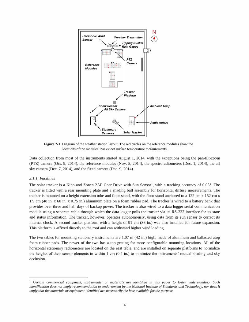
station layout is shown in Figure 2-1.
4
Figure 2-1 Diagram of the weather station layout. The red circles on the reference modules show the
locations of the modules’ backsheet surface temperature measurements.
Data collection from most of the instruments started August 1, 2014, with the exceptions being the pan-tilt-zoom
(PTZ) camera (Oct. 9, 2014), the reference modules (Nov. 5, 2014), the spectroradiometers (Dec. 1, 2014), the all
sky camera (Dec. 7, 2014), and the fixed camera (Dec. 9, 2014).
2.1.1. Facilities
The solar tracker is a Kipp and Zonen 2AP Gear Drive with Sun Sensor1, with a tracking accuracy of 0.05°. The
tracker is fitted with a rear mounting plate and a shading ball assembly for horizontal diffuse measurements. The
tracker is mounted on a height extension tube and floor stand, with the floor stand anchored to a 122 cm x 152 cm x
1.9 cm (48 in. x 60 in. x 0.75 in.) aluminum plate on a foam rubber pad. The tracker is wired to a battery bank that
provides over three and half days of backup power. The tracker is also wired to a data logger serial communication
module using a separate cable through which the data logger polls the tracker via its RS-232 interface for its state
and status information. The tracker, however, operates autonomously, using data from its sun sensor to correct its
internal clock. A second tracker platform with a height of 91 cm (36 in.) was also installed for future expansion.
This platform is affixed directly to the roof and can withstand higher wind loading.
The two tables for mounting stationary instruments are 1.07 m (42 in.) high, made of aluminum and ballasted atop
foam rubber pads. The newer of the two has a top grating for more configurable mounting locations. All of the
horizontal stationary radiometers are located on the east table, and are installed on separate platforms to normalize
the heights of their sensor elements to within 1 cm (0.4 in.) to minimize the instruments’ mutual shading and sky
occlusion.
1 Certain commercial equipment, instruments, or materials are identified in this paper to foster understanding. Such
identification does not imply recommendation or endorsement by the National Institute of Standards and Technology, nor does it
imply that the materials or equipment identified are necessarily the best available for the purpose.
5
The 6.1 m (20 ft) tall, 5.1 cm (2 in.) diameter mast is a Campbell Scientific CM120 with crossbeams for mounting
instruments at 1.78 m (5.8 ft) and 5.33 m (17.5 ft) above the roof. A lightning rod extends 71 cm (28 in.) above the
top of the mast, which is electrically connected through the mast and bonded to the building’s lightning ground via a
lightning wire. The mast is anchored to three 61 cm x 61 cm x 2.5 cm (24 in. x 24 in. x 1 in.) aluminum plates on
foam rubber pads with additional ballast and is supported using guy wires attached to eye bolt anchors in the roof.
The PV module platform is nominally 1.22 m (48 in.) high, with more northern modules mounted progressively
higher to reduce shading. The platform height is high enough for easily moving about under the platform and
accessing the modules’ wiring and low enough for easily installing the modules and periodically cleaning them. The
platform is constructed of extruded aluminum t-slot framing, which allows easy future reconfiguration.
Separate metal conduits are used for running signal, AC, and PV power cables to reduce electromagnetic
interference (EMI). These conduits enter the roof through a single penetration and into a large enclosure. The cables
are split off into other conduits running to pull boxes and conduit access ports at various locations on the roof, with
cable groups in the main enclosure wrapped with metal foil shielded sleeving to reduce EMI. Aluminum conduit
was chosen instead of PVC or steel to shield the cables from EMI and not rust. A second penetration has also been
installed for future expansion.
2.1.2. Shading
The weather station is arranged in a manner to minimize shading on the instruments and modules. The railing
surrounding the roof is at the minimum safe height of 1.07 m (42 in.), and this height determines the minimum
height of all of the instruments and modules in order for them to remain unshaded by the railing. The roof access
ladder and jib crane, 1.41 m (56 in.) and 1.63 m (64 in.) high, respectively, were installed in the northeast corner of
the roof to minimize their shading impact, which would occur in the summer months at sunrise.
The two tracker positions are located in the east-west middle of the roof to reduce the amount of time their longer
early morning and late evening shadows are cast on the modules north of the trackers. They are in a north-south
arrangement so they do not point at each other at sunrise and sunset and are separated by a distance that keeps the
southern tracker from shading the northern one. The two tables, each with the same height as the railing, are
arranged furthest south on both sides of the trackers to eliminate any shading on the tables coming from the south.
Aluminum instrument platforms normalize the height of the different instruments on the tables to minimize their
mutual shading and sky occlusion. The tops of these table instruments are just below the lowest sun-pointing
instruments on the tracker, allowing the tracker instruments to ‘see’ just over the table instruments to the horizon.
North of the trackers and tables is the PV module platform, with a nominal height of 1.22 m (48 in.) This platform is
positioned in the east-west middle of the roof to minimize any shading from the tracker in the early morning and late
evening. The platform is separated from the northern tracker position by a distance that keeps the tracker from
shading the closest module. Higher tilted modules are positioned north of lower tilted modules and at a
progressively higher height to eliminate shading from more southern modules.
Farthest north on the roof is the 6.1 m (20 ft) tall instrument mast. This mast is also positioned in the east-west
middle of the roof in line with the module platform. The lower crossbar positions the instruments mounted on it just
above the closest modules. This mast position and configuration minimizes its shading on the module platform.
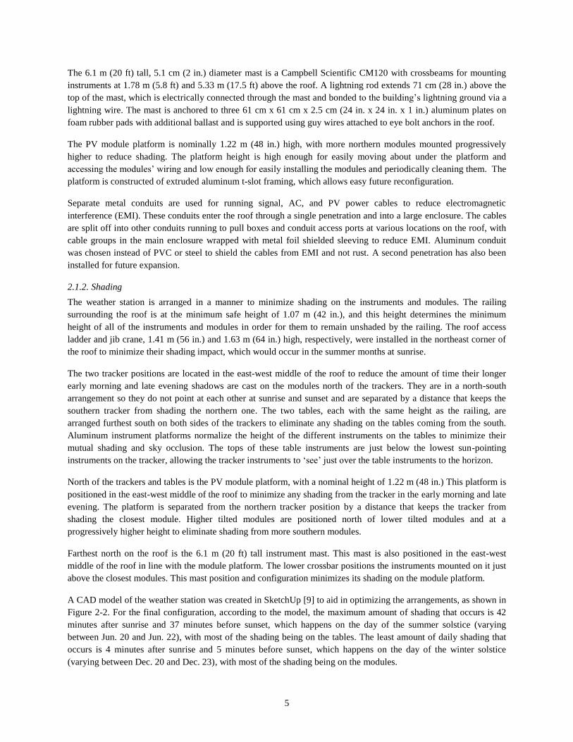
A CAD model of the weather station was created in SketchUp [9] to aid in optimizing the arrangements, as shown in
Figure 2-2. For the final configuration, according to the model, the maximum amount of shading that occurs is 42
minutes after sunrise and 37 minutes before sunset, which happens on the day of the summer solstice (varying
between Jun. 20 and Jun. 22), with most of the shading being on the tables. The least amount of daily shading that
occurs is 4 minutes after sunrise and 5 minutes before sunset, which happens on the day of the winter solstice
(varying between Dec. 20 and Dec. 23), with most of the shading being on the modules.
6
Figure 2-2 Preliminary shading model of weather station showing an unshaded period on Dec. 21 at 09:24 EST
3. Measurements
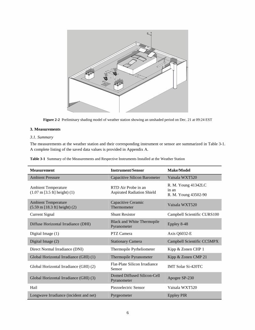
3.1. Summary
The measurements at the weather station and their corresponding instrument or sensor are summarized in Table 3-1.
A complete listing of the saved data values is provided in Appendix A.
Table 3-1 Summary of the Measurements and Respective Instruments Installed at the Weather Station
Measurement Instrument/Sensor Make/Model
Ambient Pressure Capacitive Silicon Barometer Vaisala WXT520
Ambient Temperature
(1.07 m [3.5 ft] height) (1)
RTD Air Probe in an
Aspirated Radiation Shield
R. M. Young 41342LC
in an
R. M. Young 43502-90
Ambient Temperature
(5.59 m [18.3 ft] height) (2)
Capacitive Ceramic
Thermometer Vaisala WXT520
Current Signal Shunt Resistor Campbell Scientific CURS100
Diffuse Horizontal Irradiance (DHI) Black and White Thermopile
Pyranometer Eppley 8-48
Digital Image (1) PTZ Camera Axis Q6032-E
Digital Image (2) Stationary Camera Campbell Scientific CC5MPX
Direct Normal Irradiance (DNI) Thermopile Pyrheliometer Kipp & Zonen CHP 1
Global Horizontal Irradiance (GHI) (1) Thermopile Pyranometer Kipp & Zonen CMP 21
Global Horizontal Irradiance (GHI) (2) Flat-Plate Silicon Irradiance
Sensor IMT Solar Si-420TC
Global Horizontal Irradiance (GHI) (3) Domed Diffused Silicon-Cell
Pyranometer Apogee SP-230
Hail Piezoelectric Sensor Vaisala WXT520
Longwave Irradiance (incident and net) Pyrgeometer Eppley PIR

7
Module Backsheet Surface Temperature (1) RTD, 4-wire, class A, 100 Ω Omega SA1-RTD-4W-80
Module Backsheet Surface Temperature (2) Thermocouple, Type T Omega CO1-T-72
Plane-of-Array (POA) Irradiance Flat-Plate Silicon Irradiance
Sensor IMT Solar Si-420TC
Rain (1) Piezoelectric Sensor Vaisala WXT520
Rain (2) and Precipitation Liquid Content Heated Tipping Bucket Rain
Gauge R. M. Young 52202
Reference Module (1) PV Module Powerlight PowerGuard*
Reference Module (2) PV Module Sharp NU-U235F2
Reference Module (3) PV Module Sunpower SPR-320E-WHT-D
Reference Module I-V Curve and Maximum
Power Point
I-V Curve Tracer with
Maximum Power Tracker and
Load
Daystar Multi-Tracer 5
Relative Humidity Capacitive Thin Film Polymer
Hygrometer Vaisala WXT520
RTD Current Shunt Resistor Campbell Scientific
4WPB100
Snow Depth Sonic Ranging Sensor Campbell Scientific SR50A
Spectral Irradiance (1) Spectroradiometer EKO MS-710
Spectral Irradiance (2) Spectroradiometer EKO MS-712
Thermocouple Reference Temperature UTR with RTD Campbell Scientific AM25T
UV Total Irradiance UV Radiometer Eppley TUVR
UV-A Irradiance UV Radiometer EKO MS-210A
UV-B Irradiance UV Radiometer EKO MS-212W
Voltage Signal Data Logger Campbell Scientific
CR1000-ST
Wind Speed and Direction
(5.72 m [18.8 ft] height) (1) Ultrasonic Wind Sensor Vaisala WXT520
Wind Speed and Direction
(2.51 m [8.3 ft] height) (2) Ultrasonic Wind Sensor Vaisala WS425
* The module itself without the mounting is a Siemens SP150-CPL
Unless noted otherwise, the instruments and sensors are wired directly to one of the data loggers, multiplexers, or
serial communication modules using UV and moisture protected cables run through metal dedicated data conduit,
separating them from power conductors that may generate high EMI. The cables enter the conduit through cable
glands at pull boxes or conduit access ports. The instruments and sensors are wired using twisted-pair or, if carrying
multiple sensor signals and/or the instruments power, twisted multi-conductor cable. The cables are shielded and
grounded at one end on the data logger side to reduce and allow the EMI to be later rejected when differentially
measured, which is especially important for the ~10 µV resolution analog voltage output of the thermopile
radiometers.

8
3.2. Global Shortwave Irradiance
3.2.1. Sensors
The global horizontal irradiance (GHI) is measured using two redundant Kipp & Zonen CMP 21 thermopile
pyranometers, an IMT Solar Si-420TC flat-plate silicon irradiance sensor, and an Apogee SP-230 domed diffused
silicon-cell pyranometer. The plane-of-array (POA) irradiance of each of the installed reference modules are also
measured using the same IMT Solar flat-plate irradiance sensor. The thermopile pyranometers are all-black sensor,
secondary-standard pyranometers. The flat-plate silicon sensors are a shunted monocrystalline silicon cell under a
thin glass cover with a cell temperature-compensated output signal. The domed diffused silicon-cell pyranometer
functions very similarly to the flat-plate irradiance sensors, but has a dome-shaped diffuser over the cell that
minimizes reflective losses.
Thermopile pyranometers were installed to most accurately measure the GHI and to be consistent with the
traditional method of measuring the GHI, allowing better comparisons to be made with other measurements. These
specific pyranometers were also chosen because they have an integrated thermistor measuring the case temperature,
which can be used to correct for the temperature dependency of the instrument’s responsivity to obtain more
accurate irradiance measurements. Two redundant pyranometers are installed, connected to separate data loggers, to
maximize data availability and to provide comparative checks of the measurements. Flat-plate silicon irradiance
sensors were installed to capture the irradiance under fast changing conditions at nearly instantaneous speeds, unlike
the pyranometers which have multiple-second response times. The flat-plate irradiance sensors, when mounted in
the modules’ respective planes, also better approximate the modules’ effective irradiances, or that absorbed by the
PV cells, because they have similar reflective properties due to the flat glass covers and similar spectral responses
since both utilize monocrystalline silicon cells. Pyranometers, in comparison, measure the incident irradiance. The
domed diffused silicon-cell pyranometer was installed because, like the flat-plate irradiance sensors, it captures fast
changing irradiance, but unlike those sensors it measures the incident, rather than the absorbed, irradiance.
These types of instruments were also chosen because they are either the same, or functionally the same sensors
installed at the campus PV arrays, which will allow better comparisons to be made with the latter measurements.
The pyranometers at the arrays are also all-black sensor, secondary standard pyranometers, the flat-plate irradiance
sensors are the exact same, and the silicon pyranometers are also the exact same except that the one at the weather
station has an integrated heater to prevent snow and ice from occluding the sensor.
3.2.2. Calibrations
All thermopile pyranometers are replaced every year with ones that have been newly calibrated at the National
Renewable Energy Laboratory (NREL) according to their Broadband Outdoor Radiometer Calibration (BORCAL)
procedure [10]. This calibration provides net-IR corrected responsivities (μV/(W·m-2)) at every 2° in the measured
solar zenith angle range. The silicon sensors were calibrated in a solar simulator at the factory and verified to be
within specifications. The flat-plate irradiance sensors have a stated yearly drift of 0.5 %, and the domed diffused
silicon pyranometers have a yearly drift of less than 2 %.
3.2.3. Locations and Orientations
The instruments measuring the GHI are located on the east of the two tables, as shown in Figure 3-1. As described in
section 2.1.1 Facilities, all radiometers on the east table are aligned vertically to normalize the heights of their sensor
elements to within 1 cm (0.4 in.) to minimize the instruments’ mutual shading and sky occlusion. All pyranometers
are oriented with their connectors facing away from the equator (north), as is the standard practice and also how they
were oriented during calibration. The flat-plate silicon irradiance sensor is oriented with its connector facing west to
replicate the landscape orientation of these sensors in the arrays.

9
Figure 3-1 The east table, looking north, with the GHI measuring pyranometers and silicon irradiance sensor
mounted on it. Also shown are the spectroradiometers, UV radiometers, and the ambient
temperature sensor (upper right).
The flat-plate silicon irradiance sensors measuring the POA irradiances are located in the respective module planes,
next to a north, high corner of the module, as shown in Figure 3-2, except for the sensor for the horizontal module,
which is the one located on the east table. These sensors are oriented with their connectors facing toward the top of
the module, which is north except for those for the two east and west facing modules, with their connectors facing
west and east, respectively.
Figure 3-2 Flat-plate silicon irradiance sensors measuring the POA irradiances on their respective reference
modules
3.2.4. Mounting and Alignment
The two Kipp & Zonen CMP 21 thermopile pyranometers are mounted in Kipp & Zonen CVF 3 ventilators. These
ventilators blow heated air up and over the pyranometers, which reduces the dirt, dew, frost, and snow buildup on

10
the glass domes. This airflow also reduces the ‘Zero Offset Type A’ bias uncertainty of the irradiance measurement
by reducing the temperature difference between the body and glass dome of the instrument. The domed diffused
silicon-cell pyranometer is mounted on an Apogee AL-100 leveling plate, and the flat-plate silicon irradiance sensor
is mounted using a custom-made mount. The flat-plate silicon sensors measuring the POA irradiances are mounted
next to their respective reference modules using Campbell Scientific CM245 Adjustable-Angle Mounting Stands.
The pyranometers are leveled using their integrated bubble levels, ensuring that the bubble is in the middle of the
center circle, with the bubble anywhere in the circle corresponding to a leveling accuracy of approximately ±0.1° for
the Kipp & Zonen CMP 21’s and ±0.4° for the Apogee SP-230 on its AL-100 leveling plate. The GHI and POA flat-
plate irradiance sensors are aligned to horizontal and the module tilts, respectively, using a Mitutoyo Pro 360
inclinometer to a reading within ±0.1°.
3.2.5. Wiring
The GHI measuring instruments are wired as described in section 3.1, except for the flat-plate irradiance sensors,
which are similarly wired using shielded twisted three-wire cable. These silicon sensors communicate over an
unpowered 4 mA to 20 mA current loop, which has a low sensitivity to electrical noise, and runs on one pair, with
the third wire supplying power to the temperature compensation and loop transmitter circuits.
3.3. Direct and Diffuse Shortwave Irradiance
3.3.1. Sensors
The direct normal irradiance (DNI) is measured using two redundant Kipp & Zonen CHP 1 pyrheliometers. The
diffuse horizontal irradiance (DHI) is measured using two redundant Eppley 8-48 pyranometers. The former are first
class thermopile pyrheliometers and the latter are black and white thermopile pyranometers.
These two types of instruments were installed to most accurately measure the DNI and DHI and to be consistent
with the traditional methods of measuring these values, therefore allowing direct comparisons with other
measurements. These specific pyrheliometers were also chosen because they have integrated temperature sensors
measuring the case temperature, which can be used to correct for the temperature dependency of the instrument’s
responsivity to obtain more accurate irradiance measurements. Thermopile pyranometers with black and white
sensors were chosen instead of those with all-black sensors because they have negligible Zero Offset Type A biases,
which are significant for all-black thermopile pyranometers when shaded. The negligible bias of the black and white
pyranometers is due to their hot and cold junctions being in the same thermal environment. Like the GHI measuring
thermopile pyranometers, redundant pyrheliometers and diffuse-measuring pyranometers are installed, connected to
separate data loggers, to maximum data availability and to provide comparative checks of the measurements.
3.3.2. Calibrations
Like the GHI measuring pyranometers, the pyrheliometers are replaced every year with ones that have been newly
calibrated at NREL according to their BORCAL procedure [10]. This calibration also provides net-IR corrected
responsivities (μV/(W·m-2)) for pyrheliometers at every 2° in the measured solar zenith angle range. The diffuse-
measuring pyranometers are replaced every year with ones that have been newly calibrated by the manufacturer in
an integrating sphere.
3.3.3. Locations and Orientations
The pyrheliometers and diffuse-measuring pyranometers are both located on the same Kipp & Zonen 2AP Gear
Drive with Sun Sensor solar tracker, as shown in Figure 3-3 and described in section 2.1.1 Facilities. The
pyranometers are oriented with their connectors facing away from the sun.

11
3.3.4. Mounting and Alignment
The pyrheliometers are mounted on the tracker’s side mounting plates and the diffuse-measuring pyranometers are
mounted on the tracker’s rear mounting plate in Eppley VEN ventilators that blow unheated air up and over the
pyranometers, which reduces the dirt, dew, frost, and snow buildup on the glass domes. These ventilators have direct
current (DC) instead of alternating current (AC) fans to minimize any EMI induced in the pyranometer sensor
cables.
Figure 3-3 The pyrheliometers mounted on the solar tracker above the sun sensor and below the horizontal
diffuse-measuring pyranometers (left and right) and IR measuring pyrgeometer (center). The
black balls shade the three horizontal instruments.
The tracker is leveled using its integrated bubble level, ensuring that the bubble is in the middle of the center circle.
The pyrheliometers are aligned to each other and to the sun sensor according to the tracker instructions. The diffuse-
measuring pyranometers are leveled using their integrated bubble levels, also ensuring that the bubble is in the
middle of the center circle, with the bubble anywhere in the circle corresponding to a leveling accuracy of
approximately ±0.2°. The shading balls are positioned so the pyranometers’ sensor elements are in the center of their
shadows at solar noon, when the shadows are smallest. The solar tracker’s sun tracking accuracy is <0.05°, which is
within the required accuracy of 0.75° for getting a full response from these model pyrheliometers [11] and well
within that needed to keep the shading balls centered over the diffuse-measuring pyranometers.
3.4. Longwave Irradiance
The incident and net horizontal longwave irradiance is measured using an Eppley Precision Infrared Radiometer
(PIR). This pyrgeometer was chosen because it has historically been one of the most popular in climate research and
has class-leading specifications. The case temperature is measured using an integrated thermistor to calculate the
instrument’s emitted IR and subsequently the incident IR from the net IR measurement. The dome temperature is
not measured.
The pyrgeometer is replaced every 18 months with one that has been newly calibrated outdoors at NREL. The
pyrgeometer is mounted on the solar tracker between the diffuse pyranometers in an Eppley VEN ventilator, as
shown in Figure 3-3, oriented with the connector facing away from the sun. Like those for the diffuse pyranometers,
this ventilator blows unheated air up and over the pyrgeometer to reduce the dirt, dew, frost, and snow buildup on
the instrument dome. This ventilator also has a DC fan to minimize any EMI induced in the sensor cable.

12
The pyrgeometer is leveled using its integrated bubble level to an accuracy of approximately ±0.2° and is shaded in
the same manner as the diffuse pyranometers. Shading the pyrgeometer reduces heating of its dome and the
correction needed for the associated signal bias.
3.5. UV Irradiance
The UV irradiance is measured using an EKO MS-210A, an EKO MS-212W, and an Eppley TUVR. The EKO MS-
210A measures the UV-A irradiance in the spectral range of 315 nm to 400 nm, the EKO MS-212W measures the
UV-B irradiance in the spectral range of 280 nm to 315 nm, and the Eppley TUVR measures the total UV irradiance
in the spectral range of 295 nm to 385 nm. The total UV irradiance measurement is mostly redundant, which helps
to maximize data availability and provide comparative checks with the other UV measurements. The UV-A and UV-
B radiometers are calibrated outdoors every 18 months by a commercial testing laboratory; the UV total radiometer
is replaced every 18 months with one that has been newly calibrated by the manufacturer. The UV radiometers are
located on the east table alongside the other stationary radiometers and oriented with their connectors facing away
from the equator (north), as shown in Figure 3-1. They are mounted horizontally and are leveled using their
respective integrated bubble levels, ensuring that the bubble is in the middle of the center circle, with the bubble
anywhere in the circle corresponding to an unspecified accuracy for the UV-A and UV-B radiometers and to an
accuracy of approximately ±0.2° for the UV total radiometer. The radiometers are wired to converter boxes in an
indoor enclosure, which power the radiometers and output analog signals proportional to the measured irradiances.
3.6. Spectral Irradiance
The spectral irradiance is measured using an EKO MS-710 spectroradiometer and an EKO MS-712
spectroradiometer. The MS-710 measures in the nominal spectral range of 350 nm to 1000 nm in 0.7 nm to 0.8 nm
increments and the MS-712 measures in the nominal spectral range of 900 nm to 1700 nm in 1.9 nm to 1.4 nm
increments. These spectroradiometers were chosen because they have class-leading specifications for continuous
outdoor measuring instruments.
The spectroradiometers are calibrated every 18 months indoors in a NIST laboratory designed for such calibrations.
The calibrations are performed using the NIST-calibrated spectral irradiance standard 1000 W FEL lamp [12], with
the lamp optically aligned 50 cm from the instruments’ diffuser. The spectral irradiance responsivities of the
spectroradiometers are calibrated using the known spectral irradiance of the lamp and are stored as calibration
functions in the instruments.
The spectroradiometers are located on the east table alongside the other stationary radiometers and oriented with
their connectors facing away from the equator (north), as shown in Figure 3-1. They are mounted horizontally and
are leveled using their respective integrated bubble levels, ensuring that the bubble is in the middle of the center
circle, with the bubble level accuracies unspecified. The spectroradiometers are wired to indoor converter boxes,
which power the spectroradiometers and relay the measurements using RS-232 serial communications connections.
3.7. Ambient Temperature
3.7.1. Sensors
The outdoor ambient air temperature is measured using an R. M. Young 41342LC 1000 Ω platinum resistance
temperature detector (RTD) probe and transducer in an R. M. Young 43502-90 aspirated radiation shield. The
radiation shield is used to shield the temperature probes from radiative heat transfer from the sun and surroundings,
which would affect the temperature of the probe, while still allowing ambient airflow around the probe. An
aspirated, or fan ventilated, radiation shield was used instead of a passively-ventilated shield to minimize stagnant
air around the probe, resulting in more accurate and responsive measurements. The backup power system also has
the capacity for an aspirated shield, unlike the smaller systems at the campus PV DASs where fanless passively-
ventilated shields are used.
13
The outdoor ambient air temperature is also measured by a Vaisala WXT520 weather transmitter. This instrument
has a capacitive ceramic thermometer inside of multi-plate passively ventilated radiation shield. The weather
transmitter is configured to sample temperature readings at 4 Hz and average every 1 s. It communicates over one
wire pair using an RS485 serial ASCII protocol at 19200 bits per second (bps).
3.7.2. Calibrations
Both sets of ambient temperature sensors were calibrated at the factory and verified to be within specifications, and
their yearly drift is unspecified.
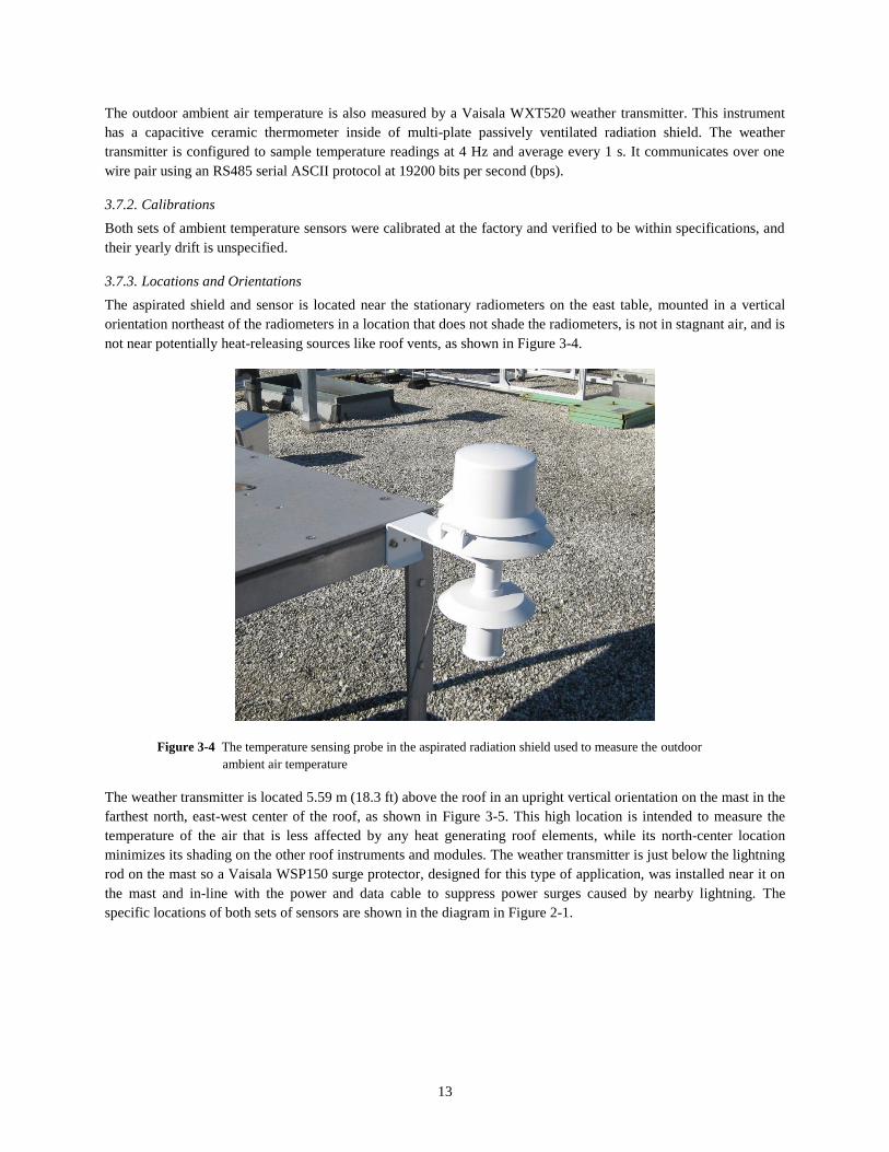
3.7.3. Locations and Orientations
The aspirated shield and sensor is located near the stationary radiometers on the east table, mounted in a vertical
orientation northeast of the radiometers in a location that does not shade the radiometers, is not in stagnant air, and is
not near potentially heat-releasing sources like roof vents, as shown in Figure 3-4.
Figure 3-4 The temperature sensing probe in the aspirated radiation shield used to measure the outdoor
ambient air temperature
The weather transmitter is located 5.59 m (18.3 ft) above the roof in an upright vertical orientation on the mast in the
farthest north, east-west center of the roof, as shown in Figure 3-5. This high location is intended to measure the
temperature of the air that is less affected by any heat generating roof elements, while its north-center location
minimizes its shading on the other roof instruments and modules. The weather transmitter is just below the lightning
rod on the mast so a Vaisala WSP150 surge protector, designed for this type of application, was installed near it on
the mast and in-line with the power and data cable to suppress power surges caused by nearby lightning. The
specific locations of both sets of sensors are shown in the diagram in Figure 2-1.

14
Figure 3-5 The weather transmitter near the top of the instrument mast
3.7.4. Wiring
The weather transmitter is wired to the surge protector, and this surge protector and the aspirated temperature sensor
are wired directly to a data logger serial communication module and multiplexer, respectively. The aspirated
temperature sensor communicates via a transducer over a powered 4 mA to 20 mA current loop, which has a low
sensitivity to electrical noise and also supplies power to the sensor.
The weather transmitter communicates over one wire pair, with power for the sensors and the heater on separate
wire pairs. To reduce power consumption, termination resistors are not wired in parallel at the ends of the RS485
communication wires to reduce signal reflections because they are not needed, as the cable lengths are less than
600 m (2000 ft) and the data rates are relatively low (19200 bps). The surge protector for this sensor is grounded to
the building’s lighting ground via the mast and lightning wire.
3.8. Wind
3.8.1. Sensors
The horizontal wind speed and direction are measured using a Vaisala WXT520 weather transmitter having a heated
ultrasonic wind sensor and a Vaisala WS425 ultrasonic wind sensor. Ultrasonic sensors were chosen instead of
traditional vane and cup or windmill anemometers because they have a smaller physical profile, are easily heated
and kept free of snow and ice, have no moving parts and therefore a higher reliability, and have a higher sensitivity
because of the faster response time and virtually zero starting threshold (even very low wind speeds are detected).
The weather transmitter is configured to sample wind readings at 4 Hz and average them every 1 s, and to perform
maximum and minimum calculations instead of gust and lull. The weather transmitter controls its level of heating as
a function of the ambient and its internal temperatures. It communicates over one wire pair using an RS485 serial
ASCII protocol at 19200 bps.
The other ultrasonic wind sensor is configured to sample readings at 1 Hz and perform no averaging. This sensor is
not heated and communicates over three wires using two analog voltage signals. The signals are 0 V to 1 V and 0 V
to the supplied reference voltage, proportional to the wind speed and direction, respectively. The reference voltage is
approximately 1.5 V, which is supplied by the datalogger via a custom voltage divider connected to one of the
datalogger’s power output terminals. The reference voltage is measured after each wind direction measurement.

15
3.8.2. Calibrations
The sensors were calibrated at the factory and verified to be within specifications, and they have an unspecified
yearly drift.
3.8.3. Locations and Orientation
The weather transmitter is located on a mast crossarm in an upright vertical orientation, with its wind transducers
5.72 m (18.8 ft) above the roof and 36 cm (14 in.) west of the mast, in the farthest north, east-west center of the roof,
as shown in Figure 3-5. This high location aims to measure close to the free-stream wind, while its north-center
location minimizes its shading on the other roof instruments and modules. The wind at this height, however, is most
likely still affected by the building. The other ultrasonic wind sensor is located on a lower mast crossarm in an
upright vertical orientation, with its transducers 2.51 m (8.3 ft) above the roof and 84 cm (33 in.) west of the mast, as
shown in Figure 3-6. The transducers are positioned 33 cm (13 in.) above the top of the highest, farthest north
reference modules and 90 cm (35.5 in.) behind them. This location aims to measure the wind that is near to but out
of the immediate boundary layer of the modules while minimally shading the modules.
Figure 3-6 The lower ultrasonic wind sensor (left) and heated tipping bucket rain gauge (right) on the lower
instrument mast crossarm
3.8.4. Mounting and Alignment
The wind sensors are mounted on top of vertical poles, aligned to true north using visual references and checked
with a compass (adjusted for the local magnetic declination). Metal spikes designed for this specific sensor are
installed on top of the weather transmitter to deter birds from perching on it and affecting the readings. The lower
ultrasonic wind sensor has no surge protector or metal spikes installed.
3.8.5. Wiring
The wiring of the weather transmitter is described in section 3.7.4. The lower ultrasonic wind sensor is wired
directly to the data logger and communicates over two wires and a common ground, with power supplied using a
separate wire pair.
3.9. Ambient Pressure and Humidity
The ambient pressure and relative humidity are also measured using the aforementioned Vaisala WXT520 weather
transmitter. The capacitive silicon pressure and capacitive thin film polymer humidity sensors are located in the

16
instrument’s passively-ventilated radiation shield. The sensors are calibrated at the factory and verified to be within
specifications, and have an unspecified yearly drift; they are replaced every 18 months. The sensors are located
5.59 m (18.3 ft) above the roof in an upright vertical orientation on the mast in the farthest north, east-west center of
the roof, as shown in Figure 3-5. This high location aims to measure the humidity of the air that is less affected by
any roof vents, while its north-center location minimizes its shading on the other roof instruments and modules. The
weather transmitter is configured to sample ambient pressure and humidity readings at 4 Hz and average them every
1 s. The wiring of the weather transmitter is described in section 3.7.4.
3.10. Precipitation
3.10.1. Liquid
3.10.1.1. Sensors
Liquid precipitation is measured using an R. M. Young 52202 rain gauge and a Vaisala WXT520 weather
transmitter. The R. M. Young 52202 is a tipping bucket rain gauge that is heated to also measure the liquid content
of snow, sleet, hail, and freezing rain. It has a 200 cm2 (31 in2) catchment area, or 16 cm (6.3 in.) diameter, with a
0.1 mm (4 mil) resolution. The weather transmitter has a horizontal steel surface on top of the instrument that is
connected to a piezoelectric sensor that measures the frequency and magnitude of raindrop impacts. The instrument
correlates the magnitude of these impacts to the volume of the rain drops. The weather transmitter is configured to
record accumulated rainfall depth.
The tipping bucket rain gauge was chosen because it is a traditional means of measuring rainfall, while the
piezoelectric sensor provides a higher resolution and faster response time than the tipping bucket gauge.
3.10.1.2. Calibrations
Both instruments were calibrated at the factory and verified to be within specifications, and they have an unspecified
yearly drift.
3.10.1.3. Locations and Orientations
The tipping bucket gauge is located on a mast crossarm, with its catchment opening 2.31 m (7.6 ft) above the roof,
84 cm (33 in.) east of the mast and 90 cm (35.5 in.) north of the northern-most reference module, as shown in Figure
3-6. The piezoelectric sensor is located 5.69 m (18.7 ft) above the roof on a mast crossarm, 36 cm (14 in.) west of
the mast. Both are mounted on top of vertical poles and aligned vertically, and both have spikes installed on top to
deter birds from perching on and fouling them and affecting their readings.
3.10.1.4. Wiring
The tipping bucket rain gauge and weather transmitter are wired as described in section 3.1 and section 3.7.4,
respectively.
3.10.2. Solid
3.10.2.1. Sensors
Snow depth is measured using a Campbell Scientific SR50A sonic ranging sensor, hail is measured using a Vaisala
WXT520 weather transmitter, and the liquid content of all solid precipitation is measured using the R. M. Young
52202 heated rain gauge described in section 3.10.1. The snow sensor measures the distance from the sensor to the
roof with the snow depth calculated as the difference between the height of the sensor and the measured distance.
The measured ambient temperature is required to correct the readings for speed-of-sound variations. The hail sensor
on the weather transmitter is the same sensor that measures the rain; it is a horizontal steel surface connected to a
piezoelectric sensor that measures the frequency of impacts. It distinguishes between hail and rain impacts, but only
counts the frequency of the hail impacts. The area of this steel surface is 60 cm2 (9.3 in2).
17
The snow sensor is configured to sample readings every 30 seconds. It uses the ambient temperature measured by
the closer aspirated temperature sensor to correct the readings. The weather transmitter is configured to record the
accumulated number of hail impacts.
3.10.2.2. Calibrations
The sensors were calibrated at the factory and verified to be within specifications, and they have unspecified yearly
drifts.
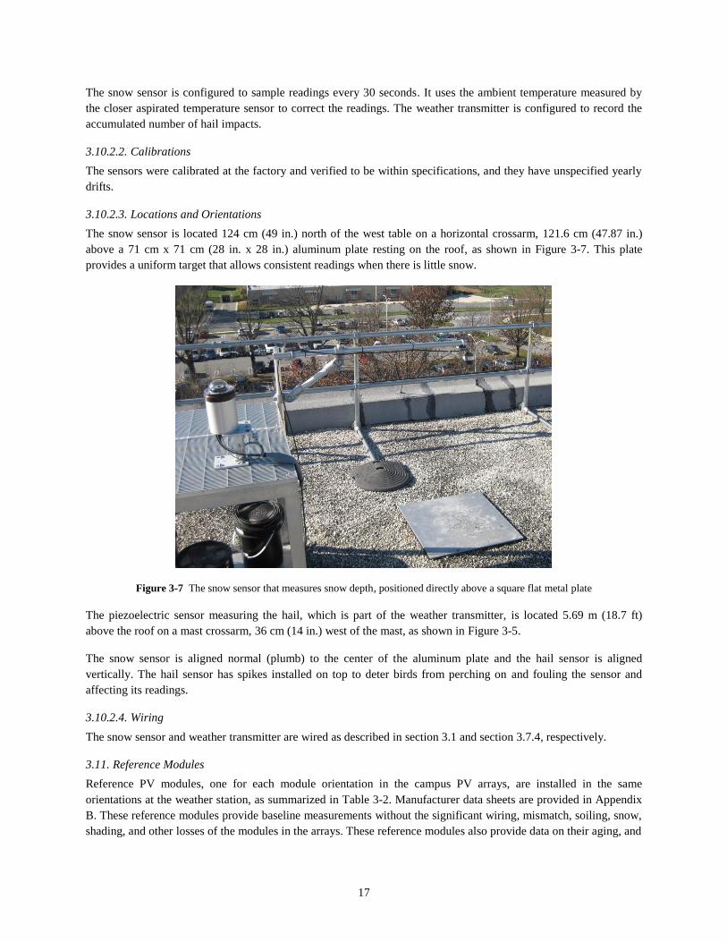
3.10.2.3. Locations and Orientations
The snow sensor is located 124 cm (49 in.) north of the west table on a horizontal crossarm, 121.6 cm (47.87 in.)
above a 71 cm x 71 cm (28 in. x 28 in.) aluminum plate resting on the roof, as shown in Figure 3-7. This plate
provides a uniform target that allows consistent readings when there is little snow.
Figure 3-7 The snow sensor that measures snow depth, positioned directly above a square flat metal plate
The piezoelectric sensor measuring the hail, which is part of the weather transmitter, is located 5.69 m (18.7 ft)
above the roof on a mast crossarm, 36 cm (14 in.) west of the mast, as shown in Figure 3-5.
The snow sensor is aligned normal (plumb) to the center of the aluminum plate and the hail sensor is aligned
vertically. The hail sensor has spikes installed on top to deter birds from perching on and fouling the sensor and
affecting its readings.
3.10.2.4. Wiring
The snow sensor and weather transmitter are wired as described in section 3.1 and section 3.7.4, respectively.
3.11. Reference Modules
Reference PV modules, one for each module orientation in the campus PV arrays, are installed in the same
orientations at the weather station, as summarized in Table 3-2. Manufacturer data sheets are provided in Appendix
B. These reference modules provide baseline measurements without the significant wiring, mismatch, soiling, snow,
shading, and other losses of the modules in the arrays. These reference modules also provide data on their aging, and
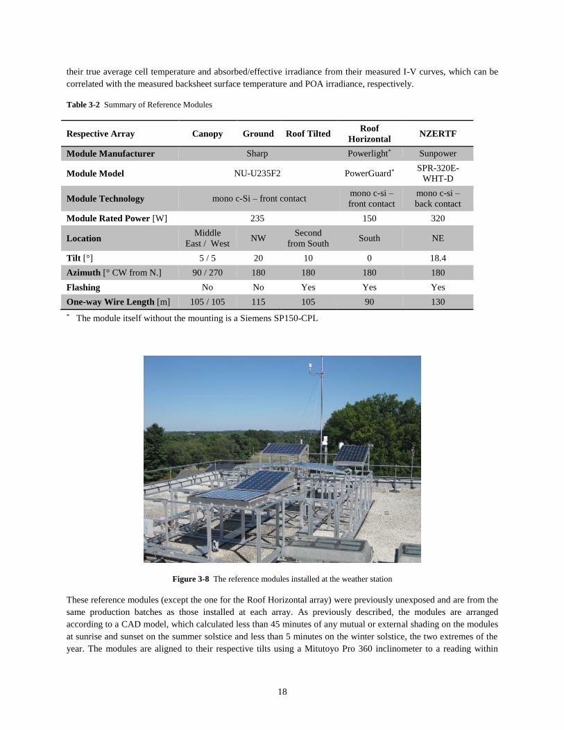
18
their true average cell temperature and absorbed/effective irradiance from their measured I-V curves, which can be
correlated with the measured backsheet surface temperature and POA irradiance, respectively.
Table 3-2 Summary of Reference Modules
Respective Array Canopy Ground Roof Tilted Roof
Horizontal NZERTF
Module Manufacturer Sharp Powerlight* Sunpower
Module Model NU-U235F2 PowerGuard* SPR-320E-
WHT-D
Module Technology mono c-Si – front contact mono c-si –
front contact
mono c-si –
back contact
Module Rated Power [W] 235 150 320
Location Middle
East / West NW
Second
from South South NE
Tilt [°] 5 / 5 20 10 0 18.4
Azimuth [° CW from N.] 90 / 270 180 180 180 180
Flashing No No Yes Yes Yes
One-way Wire Length [m] 105 / 105 115 105 90 130
* The module itself without the mounting is a Siemens SP150-CPL
Figure 3-8 The reference modules installed at the weather station
These reference modules (except the one for the Roof Horizontal array) were previously unexposed and are from the
same production batches as those installed at each array. As previously described, the modules are arranged
according to a CAD model, which calculated less than 45 minutes of any mutual or external shading on the modules
at sunrise and sunset on the summer solstice and less than 5 minutes on the winter solstice, the two extremes of the
year. The modules are aligned to their respective tilts using a Mitutoyo Pro 360 inclinometer to a reading within

19
±0.2°, and are aligned to their respective azimuths using visual references and checked with a compass (adjusted for
the local magnetic declination).
Sheet metal flashing is installed around the modules for the Roof Horizontal, Roof Tilted, and NZERTF arrays to
simulate the effect of the respective installations on the module temperatures; the modules in the Canopy and
Ground Arrays have open air circulation on their back sides and therefore have no flashing installed around their
reference modules.
The POA irradiance on each module is measured using flat-plate silicon irradiance sensors, as described in section
3.2, and the backsheet surface temperatures of each module are measured at multiple locations using RTDs and
thermocouples, as described in section 3.12. The modules are wired directly to an indoor I-V curve tracer with
maximum power tracker and load using 10 AWG (5.26 mm2) UV and moisture protected PV cable run through
metal dedicated conduit.
3.12. Module Temperature
3.12.1. Sensors
The reference modules’ backsheet surface temperatures are measured using Omega SA1-RTD-4W-80 RTDs and
Omega CO1-T-72 thermocouples. The RTD is an exposed, thin-film, four-wire, class “A”, 100 Ω platinum RTD
with an α = 0.00385. The sensing element is flat, with only a thin ceramic base material covering the resistive
element, thereby reducing the thermal gradient in the sensor, bringing it closer to the module surface temperature.
The RTD has a relatively small sensing area of 2 mm x 2.2 mm (0.08 in. x 0.09 in.) that results in faster response
times due to the smaller thermal mass. The RTD has a large 19 mm x 26 mm (0.75 in. x 1.0 in.) adhesive backing to
the sensing element, which provides secure mounting to the module. A four-wire RTD was chosen instead of a two
or three-wire RTD because the long cable leads, the large changes in temperature and subsequent resistance of the
sensing element, and using a static, unbalanced resistance bridge would have resulted in significant measurement
errors.
The Omega CO1-T-72 thermocouple is an ungrounded, flat, low mass, type T, ANSI “Special Limits of Error”
grade foil sensor. This temperature sensor is also flat to reduce the thermal gradient in the sensor and has a relatively
small sensing area that results in a fast response time. The thermocouple sensing element is encapsulated in a 10 mm
x 20 mm (0.4 in. x 0.8 in.) polymer laminate, which allows secure mounting to the module. A type T thermocouple
was chosen because it is the most accurate in this application’s measurement range.
The specific RTD and thermocouple models were originally chosen and installed on the modules in the arrays.
Thermocouples were installed at the Roof Horizontal and NZERTF arrays, while RTDs were installed at the
Canopy, Ground, and Roof Tilted arrays. The thermocouples were installed at the former arrays to more easily
integrate with the existing data acquisition systems, while RTDs were installed at the latter arrays because they are
the most stable and accurate temperature sensing technology [13]. RTDs also do not require a temperature reference
unlike thermocouples, which for the higher accuracy and many channel units can be rather large, and in the case of
ice point references require significant amounts of power. There is sufficient backup power and space at the former
arrays for accurate temperature references but not at the locations of the latter arrays. RTDs do, however, need
excitation, which requires a current source, increases the sampling time, and causes self-heating of the resistance
sensor that affects the measurement. These issues were addressed and minimized, as later described in the Data
Acquisition and Control section.
The same types of temperature sensors were installed on the respective reference modules in order to have the best
correlation between the array and reference module temperature measurements. This choice was also made to allow
evaluation of the sensors themselves via in-situ measurement of the reference module temperatures by alternate
means. An extra type T thermocouple of the same model was also installed in the center of every reference module

20
to connect to the built-in thermocouple temperature channels on the I-V tracer with maximum power tracker and
load and provide a temperature measurement more easily correlated with the module measurements.
The same model thermocouple is installed on the corresponding reference modules for the Roof Horizontal and
NZERTF arrays, but different model RTDs are installed at the Canopy, Roof Tilted, and Ground Arrays. At those
arrays, the Omega RTD-3-F3102-72-T was used, which is very similar to the model of RTD installed on the
reference modules, but does not have an adhesive backing and has a smaller subsequent contact area of 3.7 mm x
4.7 mm (0.147 in. x 0.185 in.). This RTD, which was installed first, was found to be relatively delicate and rather
difficult to install due to its size. A visual comparison of the three temperature sensors is shown in Figure 3-9.
Figure 3-9 A visual comparison of the three types of module temperature sensors used for the reference
modules and at the arrays: the RTD used at the Canopy, Roof Tilted, and Ground Arrays (left),
the RTD used for the corresponding reference modules (center), and the thermocouple used at
Roof Horizontal and NZERTF arrays and all of the reference modules (right).
3.12.2. Calibrations
All of the module temperature sensors were calibrated in the laboratory according to ASTM E220 [14]. According
to the standard, dry calibrations were performed, with the test and reference temperature sensors packed in brass test
tubes with thermally conductive aluminum oxide powder and immersed in a circulating temperature bath. All RTDs
and thermocouples were within specifications, and the proportional and offset calibration coefficients and associated
uncertainty were calculated for each sensor.
3.12.3. Locations
The sensors are mounted on the backsheets of the modules, with each sensor centered under a cell. Four sensors,
either all RTDs or thermocouples, are installed on each module, positioned behind one center and three peripheral
cells according to IEC 60891 [15]. The distribution of the sensors is intended to best capture temperature gradients
in the module and for best calculating a single representative module temperature. An additional thermocouple of
the same model used on other modules is also installed under a center cell.

21
3.12.4. Mounting and Alignment
The temperature sensors are mounted to the module backsheet using Omegabond OB-101 thermally conductive
epoxy and an Innotec 248DR, 57.2 mm (2.25 in.) diameter, 83 µm (3.3 mil) thick round polyester adhesive film
overlay, as shown in Figure 3-10. This method was derived as the combination of two of the best module back
surface temperature measurement methods as determined by Smith, et al. [16], specifically the methods designated
as positions C and H. This combination allows accurate measurement of the surface temperature, minimally affects
the surface temperature, results in a more precise bias from the true cell temperature, and provides reliably secure
attachment to the surface. The best practices recommended by Smith, et al. were also followed when mounting the
sensors, including minimizing the thickness of the epoxy under the sensor, minimizing the epoxy spread beyond the
sides of the sensor, and using additional adhesive films and ties on the cable for strain relief to prevent the sensor
from detaching. For the adhesive backed RTDs, the thermally conductive epoxy is applied to the adhesive surface,
first removing the adhesive covers. The temperature sensors were aligned under the center of the respective cells by
distance measurements and visual means.
Figure 3-10 An RTD mounted on the back of a module using thermally conductive epoxy and an adhesive
film overlay
3.12.5. Wiring
The module temperature sensors are wired directly to the data logger multiplexers. The RTD cable has four wires
with the inner wire insulation (and outer jacket) made of PTFE (Teflon). PTFE has a much lower permittivity and
subsequent capacitance than PVC and nearly all other wire insulation materials, resulting in faster settling times
after excitation. The RTDs are connected to the extension cables using waterproof IP67 connectors. The TCs are
connected to the extension cables using standard flat pin connectors housed in custom waterproof cable connector
enclosures.
4. Data Acquisition and Control
4.1. Data loggers
4.1.1. Components
The weather station uses two Campbell Scientific CR1000-ST data loggers, as shown in Figure 4-1.
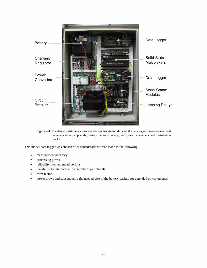
22
Figure 4-1 The data acquisition enclosure at the weather station showing the data loggers, measurement and
communication peripherals, battery backups, relays, and power converters and distribution
blocks
This model data logger was chosen after considerations were made to the following:
measurement accuracy
processing power
reliability over extended periods
the ability to interface with a variety of peripherals
form factor
power draws and subsequently the needed size of the battery backup for extended power outages
23
This data logger is also the same one chosen for the campus PV array DASs. The analog voltage, current, and
thermocouple signals are multiplexed using Campbell Scientific AM25T solid-state multiplexers. The current
carrying wires are first connected to Campbell Scientific CURS100 100 ohm current shunts to convert the current
signals to voltage signals. The thermocouples are all connected to the same (lower) multiplexer and covered with the
supplied insulated cover to reduce temperature gradients in the terminals and the resulting bias errors. These
multiplexers are also uniform temperature references (UTR) which have an integrated RTD to measure the
thermocouple reference temperature. The RTDs are multiplexed using one Campbell Scientific AM16/32B-ST relay
multiplexer, located below the lower data logger in Figure 4-1. The serial devices are each connected to separate
Campbell Scientific SDM-SIO1 serial communication modules. Redundant instruments and those measuring similar
parameters are split between the two data loggers to maximize data availability in the event that one data logger
stops operating.
Solid-state multiplexers are used because of their faster switching times and greater longevity than relay
multiplexers, as measurements are needed on numerous channels at a one-second sample rate over an extended
duration. A relay multiplexer is used for the RTD measurements instead of a solid-state multiplexer because the
solid-state multiplexers cannot pass the currents needed to excite the RTDs. This restriction does limit the RTD
sample period to greater than one-second, but this rate is acceptable because the module temperatures change at a
slower rate than the irradiance. The separate serial communication modules are used instead of the serial
communication channels on the data logger because there were not enough available channels.
The relay multiplexer is connected to the lower data logger through a Campbell Scientific 4WPB100 100 Ω four-
wire half-bridge terminal input module. The bridge employs a high-accuracy (±0.01 %), low temperature
dependence (< 8 x 10⁻⁶/°C) shunt to measure the current through the RTD, generated by the excitation voltage
supplied by the data logger. A current limiting resistor is used in series with the shunt to allow for higher excitation
voltages at the data logger, minimizing the relative noise in the excitation, while limiting the current and subsequent
self-heating in the sensing resistor (RTD). Self-heating, which results in a measurement bias error, is caused by the
excitation current passing through the sensor resistor.
A Campbell Scientific LR4 latching relay module is connected to each of the data loggers, via an SDI-12 bus
connection. The ventilator fans and heaters are connected to the relays’ terminals and power to them is controlled
via their respective data logger.
A Campbell Scientific NL115 is connected to each of the data loggers’ peripheral port and provides 10BASE-T
Ethernet communications and a CompactFlash card slot interface for storing measurement data. An industrial quality
2 GB Synchrotech CFV-2GB-TSI-3524 card is used, which, like the data logger, can operate with high reliability for
extended periods in outdoor conditions.
4.1.2. Locations and Housing
The data acquisition enclosure is located in an unconditioned room below the weather station, as shown in Figure
4-2. The enclosure is NEMA 4 rated and locked to control access, with an additional sensor installed to monitor
when the door is open (at which time the data logger sends out an email alert). The humidity in the enclosure is
regulated by sealing the conduit openings with duct seal compound and replacing desiccant packets on an as needed
basis, with the humidity level monitored using a humidity indicator card.

24
Figure 4-2 Location of the data acquisition enclosures and central UPS
Left of the main data acquisition enclosure is a smaller enclosure with clear acrylic sides that houses the EKO UV-A
and UV-B converter boxes and the power supply for the rain gauge heater. Also in the enclosure are
communications and power equipment for cameras on the roof, a network switch, and a remote power strip for
controlling the power to select components.
4.1.3. Wiring
All wiring inside of the enclosures is low capacitance, high temperature PTFE insulated stranded wires with
insulated ferrules crimped on their ends. Ferrule-terminated wires make troubleshooting and reworking easier and
provide a more secure, lower contact resistance connection to the terminals. Jumper wires are connected between the
low sides of the differential inputs and the respective ground terminals for the thermopile pyranometers,
pyrheliometers, and the UV total radiometer to keep these electrically floating sensors from floating above the
ground potential and out of the data logger’s common mode range, which would decrease the accuracy of the
measurements. The jumpers also keep these radiometers from potentially floating out of the measurable range
entirely.
The Ethernet communication module on the data loggers connect via Cat6 Ethernet patch cables directly to the NIST
network.
The data acquisition enclosure components are grounded to a central point on the enclosure. Grounding in a “star-
point” configuration minimizes the potential differences between the devices and therefore reduces any currents
through the devices during a power surge event. The central point of the “star” is connected via the enclosure to the
conduit which is locally grounded. The conduit was chosen instead of the ground wire fed from the nearby power
distribution board because it provides a lower resistance path to ground and will not have an electrical choke effect
when there is a sudden, high current surge from a nearby lightning strike, which occurs for a surge carrying wire
inside of a ferrous conduit. The importance of proper grounding in the interest of equipment longevity cannot be
overemphasized.
Four conduits connect to the data acquisition enclosure, separately carrying the AC power wires, the Ethernet
communication patch cables, the sensor data cables, and the DC power cables for the ventilators. Excess lengths of

25
the data cables for potential future reworks (approximately 3 m [10 ft]) are stored in a smaller enclosure below the
DAS enclosure in-line with the data conduit.
4.1.4. Configuration
4.1.5. Sampling Rates and Parallel Processing
The data loggers are programmed using the Campbell Scientific language CRBASIC. The programs measure all of
the sensors every 1 s, except for the RTDs and thermocouples measuring the reference modules’ temperatures,
which are measured every 10 s. The slower RTD sampling rate is due to the slower relay multiplexers to which the
RTDs are connected, but is not a restriction nonetheless because the module temperatures are not changing
appreciably faster than every 10 s. The UTR thermocouple reference temperature is measured before each set of
thermocouple measurements. It takes longer than 1 s to measure, and poll and receive data from the sensors and
instruments if done sequentially, so the program is run in “pipeline” mode which effectively executes some of the
measurement steps in parallel.
4.1.6. Time Synchronization
In order to maintain time synchronization within 1 s between data loggers, the data loggers are instructed every
morning just after midnight to synchronize with a local internet time server. This synchronization keeps the data
loggers within 0.5 s of each other at all times. The data loggers are configured to always use local standard time
(LST) to eliminate issues arising from the switch to and from daylight saving time (DST) and to allow easier
comparisons and calculations.
4.1.7. Channel Ranges
The input voltage ranges for each measurement channel are explicitly chosen and fixed; auto-range is not used to
eliminate the initial measurement needed to set the range, resulting in a shorter sampling time. The range determined
by auto-range may also not be accurate for the irradiance and electrical measurements as they can fluctuate rapidly.
4.1.8. Self-Calibration
The data loggers are instructed to periodically self-calibrate to compensate for aging-induced and operating
temperature-induced (Seebeck effect) drift. Voltage offsets are measured on each channel when the signal source is
internally disconnected, using an internal voltage standard as a reference for all channels.
4.1.9. Measurement Techniques
Various techniques are employed for every measurement to more accurately measure the sensed value. The voltage
signals, both direct from the sensor and those from a shunt when measuring current signals, are measured
differentially instead of single-ended with respect to the data logger ground. This approach eliminates any voltage
reference offsets and rejects capacitively coupled common-mode noise. The only exception to this approach is for
the signals from the lower ultrasonic wind sensor, which are inherently single-ended. Before each of these
measurements, the ground offset is measured and subtracted from the instrument signals to negate any bias.
Although considered, the electrically floating sensors are not pulled to ground before each measurement to null any
common-mode voltage. Rather, jumper wires are connected between the low sides of the differential inputs of the
radiometers and the respective ground terminals to keep them grounded. These data loggers combine nulling the
common-mode voltage with open input detection, commonly used for thermocouples, into one function and neither
can be individually implemented. The open input detection, which biases the high side of the differential input above
the channel measurement range while grounding the low side, would not allow the thermopile-based radiometers’
outputs enough time to stabilize before the measurements. No measurement channels in this DAS employ the
common-mode nulling and open input detection function, including for the thermocouples measuring the
temperature of two of the reference modules, in order to save measurement time.
26
The settling times, the delay after the channel terminals are internally connected to the input amplifier and before the
measurement is started, were chosen to be 10 ms for the thermopile-based radiometers and 3 ms for other analog
signals. The longer settling time for the thermopile-based radiometers allows further reduction of voltage transients
caused by channel switching, as they would have a larger relative magnitude since their voltage signals are much
smaller.
The voltage signals are integrated for exactly 16.67 ms. This integration time, the period of a 60 Hz waveform,
rejects 60 Hz frequency components in the signal by cancelling them out. This noise is induced from nearby AC
power sources, which operate at 60 Hz in the USA.
Each differential voltage measurement is performed twice, with the second time after the channel terminals are
internally reverse-connected to the input amplifier. The two measurements are subtracted and divided by two to
cancel any voltage offsets in the measurement circuitry, as well as any common-mode gain errors. Note that before
each measurement the signal is allowed time to settle, which doubles the total settling time per measurement.
There is not enough available time in the 1 s scan period to employ all of the aforementioned techniques when
measuring the four-wire RTDs, so tests were performed to identify those most beneficial in this application. The
tests determined that a settling time of 3 ms was adequate and revealed that 60 Hz integration reduces significantly
more noise than reversing the inputs and reversing the excitation, combined. Reversing the excitation is similar to
reversing the inputs, but does so for the excitation and works to cancel any voltage offsets before and in the
measurement circuitry (reversing the input cancels the offset in the measurement circuitry as well as the common-
mode gain errors). Note that these two techniques each double the total settling time and combining both quadruples
it. If there were a longer sampling period, then all three techniques would have been employed, even though the
benefits of the two reversals are relatively small in this application.
The excitation for the RTDs is optimized by maximizing the measurement resolution of the voltage across the
sensing resistor (RTD) while keeping the self-heating error, caused by the excitation current passing through the
sensing resistor, below an acceptable level. Self-heating errors for 100 Ω RTDs like the ones in this DAS are less
than 0.001 °C (0.0018 °F) in still air when the voltage drop across the sensing resistor is less than approximately
25 mV (6 µW) [17]. The optimal excitation voltage is therefore what results in a maximum sensor voltage of 25 mV,
which occurs at the highest expected temperature, chosen conservatively to be 90 °C (194 °F). This temperature
corresponds to a maximum resistance of 135 Ω. The optimal excitation voltage is calculated for the half-bridge and
current-limiting resistor in Figure 4-3 using Equation (1), neglecting the wire resistances. The equation is calculated
using values of the measurement bridge resistors at the low end of their respective tolerance ranges, resulting in a
higher current and subsequently higher RTD voltage. If the tolerances are not accounted for, this potentially higher
RTD voltage could be greater than the selected measurement range.

27
Figure 4-3 Half-bridge for measuring distant RTDs to nullify effect of wire resistances
,max
,min ,min ,max
,max
s
x cl sh s
s
VV R R R
R (1)
where:
Vx = excitation voltage
Vs = sensing voltage
Rs = sensing resistor (RTD)
Rcl = current limiting resistor
Rsh = completion (shunt) resistor
Vsh = shunt voltage
Ix = excitation current
The optimal excitation, calculated to be 1.8 V, is kept on only during the measurement to further reduce the self-
heating errors. The measurement equation for the half-bridge, when reduced, becomes the ratiometric relation
s sh s shR R V V . The temperature of the RTD is then determined from the resistance using the inverse of the
Callendar-Van Dusen equation according to the ASTM E1137-04 [18] standard.
Timeouts for the serial communicating instruments, the time after polling the instrument waiting for a reply, were
carefully chosen to be the maximum time the instrument normally takes to respond to a request. A flag in the data
logger programs can be manually set while the program is running to stop polling individual instruments in the case
where they are temporarily unresponsive. Setting this flag can speed up the program and avoid missed
measurements while the data logger would normally be waiting the full timeout period for a response.
4.1.10. Control
The data loggers regulate the power to the UV-A and UV-B radiometers, the rain gauge heater, the POA flat-plate
silicon irradiance sensors, the weather transmitter heater, and the fans and heaters in the ventilators when external
power to the DAS is off and the data loggers, instruments, and other equipment are operating on battery power.
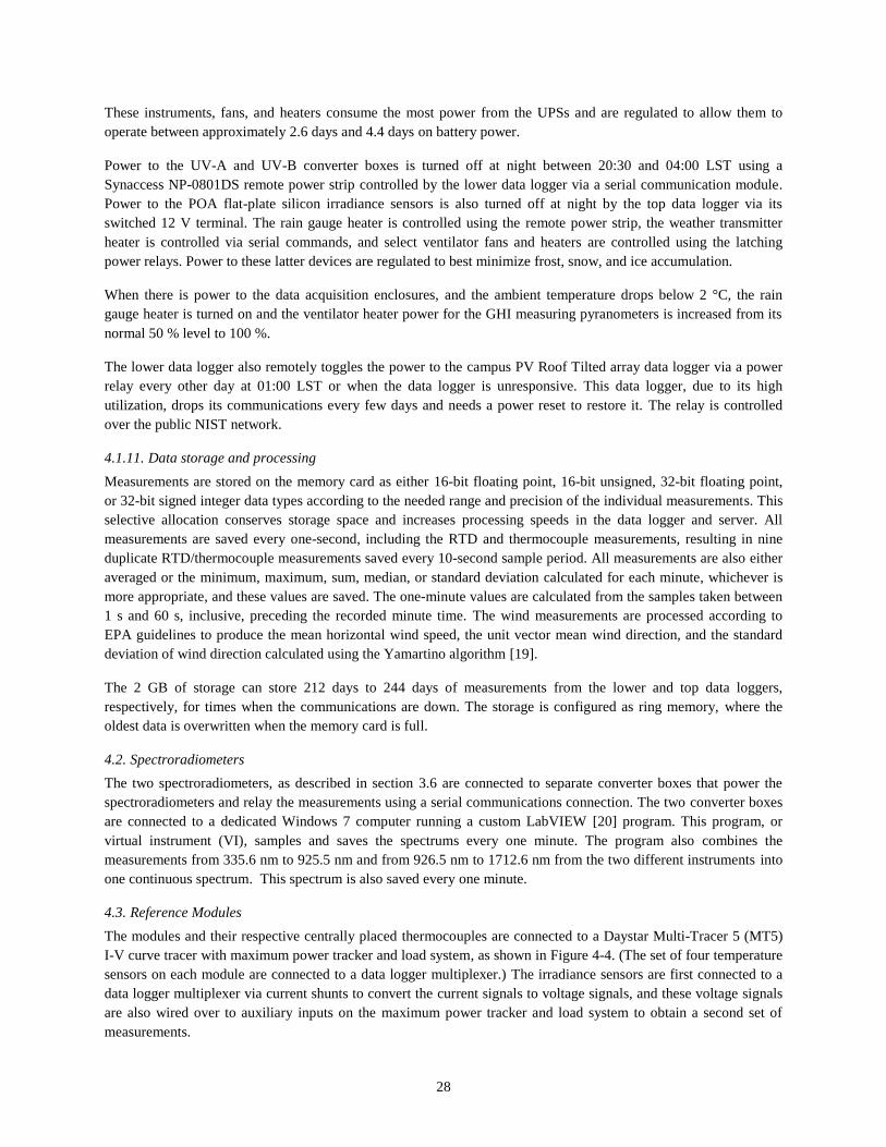
28
These instruments, fans, and heaters consume the most power from the UPSs and are regulated to allow them to
operate between approximately 2.6 days and 4.4 days on battery power.
Power to the UV-A and UV-B converter boxes is turned off at night between 20:30 and 04:00 LST using a
Synaccess NP-0801DS remote power strip controlled by the lower data logger via a serial communication module.
Power to the POA flat-plate silicon irradiance sensors is also turned off at night by the top data logger via its
switched 12 V terminal. The rain gauge heater is controlled using the remote power strip, the weather transmitter
heater is controlled via serial commands, and select ventilator fans and heaters are controlled using the latching
power relays. Power to these latter devices are regulated to best minimize frost, snow, and ice accumulation.
When there is power to the data acquisition enclosures, and the ambient temperature drops below 2 °C, the rain
gauge heater is turned on and the ventilator heater power for the GHI measuring pyranometers is increased from its
normal 50 % level to 100 %.
The lower data logger also remotely toggles the power to the campus PV Roof Tilted array data logger via a power
relay every other day at 01:00 LST or when the data logger is unresponsive. This data logger, due to its high
utilization, drops its communications every few days and needs a power reset to restore it. The relay is controlled
over the public NIST network.
4.1.11. Data storage and processing
Measurements are stored on the memory card as either 16-bit floating point, 16-bit unsigned, 32-bit floating point,
or 32-bit signed integer data types according to the needed range and precision of the individual measurements. This
selective allocation conserves storage space and increases processing speeds in the data logger and server. All
measurements are saved every one-second, including the RTD and thermocouple measurements, resulting in nine
duplicate RTD/thermocouple measurements saved every 10-second sample period. All measurements are also either
averaged or the minimum, maximum, sum, median, or standard deviation calculated for each minute, whichever is
more appropriate, and these values are saved. The one-minute values are calculated from the samples taken between
1 s and 60 s, inclusive, preceding the recorded minute time. The wind measurements are processed according to
EPA guidelines to produce the mean horizontal wind speed, the unit vector mean wind direction, and the standard
deviation of wind direction calculated using the Yamartino algorithm [19].
The 2 GB of storage can store 212 days to 244 days of measurements from the lower and top data loggers,
respectively, for times when the communications are down. The storage is configured as ring memory, where the
oldest data is overwritten when the memory card is full.
4.2. Spectroradiometers
The two spectroradiometers, as described in section 3.6 are connected to separate converter boxes that power the
spectroradiometers and relay the measurements using a serial communications connection. The two converter boxes
are connected to a dedicated Windows 7 computer running a custom LabVIEW [20] program. This program, or
virtual instrument (VI), samples and saves the spectrums every one minute. The program also combines the
measurements from 335.6 nm to 925.5 nm and from 926.5 nm to 1712.6 nm from the two different instruments into
one continuous spectrum. This spectrum is also saved every one minute.
4.3. Reference Modules
The modules and their respective centrally placed thermocouples are connected to a Daystar Multi-Tracer 5 (MT5)
I-V curve tracer with maximum power tracker and load system, as shown in Figure 4-4. (The set of four temperature
sensors on each module are connected to a data logger multiplexer.) The irradiance sensors are first connected to a
data logger multiplexer via current shunts to convert the current signals to voltage signals, and these voltage signals
are also wired over to auxiliary inputs on the maximum power tracker and load system to obtain a second set of
measurements.
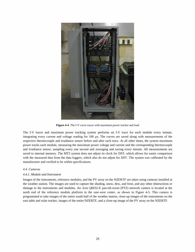
29
Figure 4-4 The I-V curve tracer with maximum power tracker and load
The I-V tracer and maximum power tracking system performs an I-V trace for each module every minute,
integrating every current and voltage reading for 100 µs. The curves are saved along with measurements of the
respective thermocouple and irradiance sensor before and after each trace. At all other times, the system maximum
power tracks each module, measuring the maximum power voltage and current and the corresponding thermocouple
and irradiance sensor, sampling every one second and averaging and saving every minute. All measurements are
saved to internal memory. The MT5 system does not adjust its clock for DST, which allows for easier comparison
with the measured data from the data loggers, which also do not adjust for DST. The system was calibrated by the
manufacturer and verified to be within specifications.
4.4. Cameras
4.4.1. Module and Instrument
Images of the instruments, reference modules, and the PV array on the NZERTF are taken using cameras installed at
the weather station. The images are used to capture the shading, snow, dew, and frost, and any other obstructions or
damage to the instruments and modules. An Axis Q6032-E pan-tilt-zoom (PTZ) network camera is located at the
north end of the reference module platform in the east-west center, as shown in Figure 4-5. This camera is
programmed to take images of the entire south half of the weather station, close-up images of the instruments on the
east table and solar tracker, images of the entire NZERTF, and a close-up image of the PV array on the NZERTF.

30
Figure 4-5 The PTZ camera that records images of the instruments and NZERTF PV array
The camera is configured for constant white balance, auto exposure, and to use an IR cut filter during the day but not
at night to increase sensitivity. The cameras, like the data loggers, are configured to not adjust their clocks for DST
for easier comparison with the measured data. The cameras take 704 x 480 resolution images, which are saved as
uncompressed JPEG images on an internal 32 GB SanDisk Extreme SD card. The cameras take images every five
minutes during the day (04:00 to 20:00 LST) and every hour all day. The camera communicates over the NIST
private network and is powered using Power over Ethernet (PoE). The midspan, for combining the power and
Ethernet, and a network switch are housed in the enclosure next to the main data acquisition enclosure, as shown in
Figure 4-2.
Two additional cameras, Campbell Scientific CC5MPXs, are located on the west table. These cameras take images
of the reference modules and view the solar tracker. The cameras do not adjust for DST and take 2592 x 1944
resolution images saved as uncompressed JPEG images on an internal 32 GB SanDisk Extreme SD card. No other
settings are configurable. The camera viewing the modules is programmed to take a fixed zoom image every five
minutes during the day (04:00 to 20:00 LST) and every hour all day; the camera viewing the solar tracker does not
currently record images. The cameras communicate over the NIST private network and are powered using separate
cables.
4.4.2. All Sky
Images of the entire sky, horizon to horizon, are taken using an all sky camera. The camera is an Alcor System
OMEA-2.0M-HCA equipped with a fisheye lens, an auto-iris, and an integrated heater. The camera CCD has an IR
cut filter and records 24 bit (8 bit dynamic range) color 1600 x 1200 resolution (2 MP) images. Paired with a
Fujinon FE185C046HA-1 fisheye lens having a 1.4 mm focal length and a 185° x 185° field of view, this camera
produces full horizon to horizon color images. However, there are unexposed areas on the sides of the image, giving
the images an effective resolution of about 1125 x 1125.
The camera has an auto-iris mechanism controlled by a photodiode that adjusts the lens aperture between F1.4 to F8
to allow nighttime, low-light, and clear sky exposures, with a typical daytime aperture setting of F5.6. An external
ambient temperature and humidity sensor is used to control an integrated heater to keep the camera dome free of fog
and frost. The camera is mounted to a custom mount that also holds the temperature and humidity sensor, as shown
in Figure 4-6.
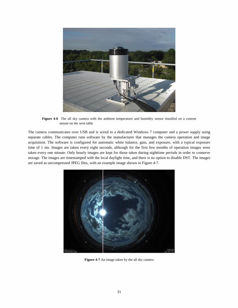
31
Figure 4-6 The all sky camera with the ambient temperature and humidity sensor installed on a custom
mount on the west table
The camera communicates over USB and is wired to a dedicated Windows 7 computer and a power supply using
separate cables. The computer runs software by the manufacturer that manages the camera operation and image
acquisition. The software is configured for automatic white balance, gain, and exposure, with a typical exposure
time of 1 ms. Images are taken every eight seconds, although for the first few months of operation images were
taken every one minute. Only hourly images are kept for those taken during nighttime periods in order to conserve
storage. The images are timestamped with the local daylight time, and there is no option to disable DST. The images
are saved as uncompressed JPEG files, with an example image shown in Figure 4-7.
Figure 4-7 An image taken by the all sky camera
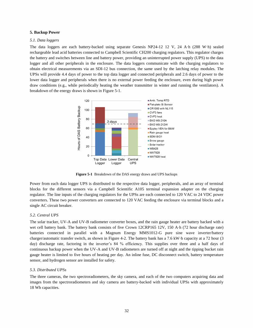
32
5. Backup Power
5.1. Data loggers
The data loggers are each battery-backed using separate Genesis NP24-12 12 V, 24 A·h (288 W·h) sealed
rechargeable lead acid batteries connected to Campbell Scientific CH200 charging regulators. This regulator charges
the battery and switches between line and battery power, providing an uninterrupted power supply (UPS) to the data
logger and all other peripherals in the enclosure. The data loggers communicate with the charging regulators to
obtain electrical measurements via an SDI-12 bus connection, the same used by the latching relay modules. The
UPSs will provide 4.4 days of power to the top data logger and connected peripherals and 2.6 days of power to the
lower data logger and peripherals when there is no external power feeding the enclosure, even during high power
draw conditions (e.g., while periodically heating the weather transmitter in winter and running the ventilators). A
breakdown of the energy draws is shown in Figure 5-1.
Figure 5-1 Breakdown of the DAS energy draws and UPS backups
Power from each data logger UPS is distributed to the respective data logger, peripherals, and an array of terminal
blocks for the different sensors via a Campbell Scientific A105 terminal expansion adapter on the charging
regulator. The line inputs of the charging regulators for the UPSs are each connected to 120 VAC to 24 VDC power
converters. These two power converters are connected to 120 VAC feeding the enclosure via terminal blocks and a
single AC circuit breaker.
5.2. Central UPS
The solar tracker, UV-A and UV-B radiometer converter boxes, and the rain gauge heater are battery backed with a
wet cell battery bank. The battery bank consists of five Crown 12CRP165 12V, 150 A·h (72 hour discharge rate)
batteries connected in parallel with a Magnum Energy MMS1012-G pure sine wave inverter/battery
charger/automatic transfer switch, as shown in Figure 4-2. The battery bank has a 7.6 kW·h capacity at a 72 hour (3
day) discharge rate, factoring in the inverter’s 84 % efficiency. This supplies over three and a half days of
continuous backup power when the UV-A and UV-B radiometers are turned off at night and the tipping bucket rain
gauge heater is limited to five hours of heating per day. An inline fuse, DC disconnect switch, battery temperature
sensor, and hydrogen sensor are installed for safety.
5.3. Distributed UPSs
The three cameras, the two spectroradiometers, the sky camera, and each of the two computers acquiring data and
images from the spectroradiometers and sky camera are battery-backed with individual UPSs with approximately
18 Wh capacities.
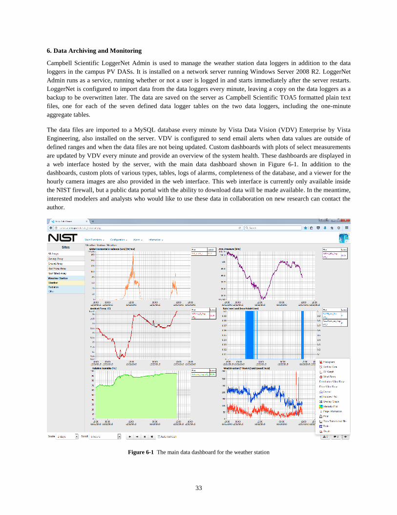
33
6. Data Archiving and Monitoring
Campbell Scientific LoggerNet Admin is used to manage the weather station data loggers in addition to the data
loggers in the campus PV DASs. It is installed on a network server running Windows Server 2008 R2. LoggerNet
Admin runs as a service, running whether or not a user is logged in and starts immediately after the server restarts.
LoggerNet is configured to import data from the data loggers every minute, leaving a copy on the data loggers as a
backup to be overwritten later. The data are saved on the server as Campbell Scientific TOA5 formatted plain text
files, one for each of the seven defined data logger tables on the two data loggers, including the one-minute
aggregate tables.
The data files are imported to a MySQL database every minute by Vista Data Vision (VDV) Enterprise by Vista
Engineering, also installed on the server. VDV is configured to send email alerts when data values are outside of
defined ranges and when the data files are not being updated. Custom dashboards with plots of select measurements
are updated by VDV every minute and provide an overview of the system health. These dashboards are displayed in
a web interface hosted by the server, with the main data dashboard shown in Figure 6-1. In addition to the
dashboards, custom plots of various types, tables, logs of alarms, completeness of the database, and a viewer for the
hourly camera images are also provided in the web interface. This web interface is currently only available inside
the NIST firewall, but a public data portal with the ability to download data will be made available. In the meantime,
interested modelers and analysts who would like to use these data in collaboration on new research can contact the
author.
Figure 6-1 The main data dashboard for the weather station

34
Data from the spectroradiometers, I-V curve tracer and maximum power tracking system, and images from the
cameras are copied to network attached storage every 30 minutes by an FTP client on the server run as a scheduled
task. A custom script, also run as a scheduled task, monitors and sends alerts when these data files are not being
transferred. VDV monitors and sends alerts when new images from each camera are not being transferred. All data
and images on the server, including data from the data loggers, are continually backed up to offsite cloud storage.
7. Uncertainty
Uncertainties for the collected data are not listed because a complete uncertainty analysis is outside the scope of this
report, but one will be presented for each measurement in a forthcoming paper. Sensor and instrument-level
uncertainties are not given as they are only part of the system-level values, and therefore can be misleading.
Furthermore, they do not account for the error between the measurand, the quantity of interest, and the realized
quantity, the quantity measurable by the sensor.
8. Maintenance
The data dashboards are checked every weekday for any apparent problems in the DAS. The irradiance sensors are
cleaned every other day, minus weekends, using cleanroom wipes moistened with a 6 % isopropyl/94 % deionized
water mixture, dried with optical tissue, and blown-off with compressed air. Any ice buildup is first melted using an
ethanol solution of the same concentration. The reference modules are cleaned on an as-needed basis. A log is kept
of the dates and times when the sensors at the different arrays are cleaned. Instrument and solar tracker level are
continually checked, as is their desiccant, and the tracker pointing accuracy is verified using the diopters on the
pyrheliometers. The rain gauge orifice is cleaned every couple weeks.
The data files on the server grow indefinitely, so once a week a custom script is run that pauses the data importation
from the data loggers and runs the Campbell Scientific program File Format Convert that splits the files into
separate daily files for easier archiving and use.
The desiccant in the data logger enclosures is checked every couple months and replaced according to the humidity
indicator in the enclosure. The solar tracker gears are greased yearly and a cold weather cover is installed over it in
the late fall and removed in the early spring. Ventilator and multi-tracer filters are replaced on a yearly basis or as
needed. Thermopile pyranometers, pyrheliometers, and the pyrgeometer are replaced every 12 to 18 months with
newly calibrated pyranometers from NREL; the UV radiometers and spectroradiometers are calibrated every 18
months. A log is kept of these instrument replacements and calibrations, which also contains all other maintenance
including when sensors, instruments, and devices fail and are replaced.
Acknowledgements
The author wishes to thank all those who contributed time and effort planning, constructing, and implementing the
infrastructure needed for the data acquisition system described in this report. Special thanks to Brian Dougherty of
NIST’s Engineering Laboratory’s (EL’s) Energy and Environment Division for logistical, construction, and
maintenance support. Thanks to Luis Luyo, also of EL’s Energy and Environment Division, for constructing the
infrastructure for the reference modules, and to Jeffrey Sze for early testing of the systems.
References
[1] Matthew Boyd, High-speed monitoring of multiple grid-connected photovoltaic array configurations, National
Institute of Standards and Technology. NIST Technical Note 1896 (2015).
http://dx.doi.org/10.6028/NIST.TN.1896
[2] A.H. Fanney, V. Payne, T. Ullah, L. Ng, M. Boyd, F. Omar, M. Davis, H. Skye, B. Dougherty, B. Polidoro, W.
Healy, J. Kneifel, and B. Pettit, Net-zero and beyond! Design and performance of NIST’s net-zero energy
residential test facility, Energy Build. 101 95–109 (2015).

35
[3] K. Lynn, SunShot, (2011). http://www.solar.energy.gov/pdfs/doe_lynn_pv_validation_2011_aug.pdf (Accessed
on Sept. 11, 2015)
[4] J. Granata, PV performance and reliability validation capabilities at Sandia National Laboratories and the
National Renewable Energy Laboratory, (2011).
http://energy.gov/sites/prod/files/2014/01/f7/pv_manufacturing_workshop_2011_march_granata.pdf
(Accessed_on Sep. 11, 2015)
[5] J. Newmiller, Validation information for PV power system project review, (2011).
http://www.solar.energy.gov/pdfs/dnv_newmiller_pv_validation_2011_aug.pdf (Accessed on Sep. 11, 2015)
[6] Sandia National Laboratories, PV validation and bankability workshop - August 31, 2011 - Survey Results,
(2011). http://energy.gov/sites/prod/files/2014/01/f7/pv_vb_surveyresults.pdf (Accessed Sep. 23, 2015)
[7] Stephen Wilcox, National solar radiation database 1991-2010 update: user’s manual, National Renewable
Energy Laboratory, (2012).
[8] NOAA, DoD, FAA, and United States Navy, Automated Surface Observing System (ASOS) User’s guide,
(1998). http://www.nws.noaa.gov/asos/pdfs/aum-toc.pdf
[9] SketchUp Pro, Trimble Navigation Limited, Sunnyvale, California USA (2012).
[10] I. Reda, D. Myers, and T. Stoffel, Uncertainty estimate for the outdoor calibration of solar pyranometers: a
metrologist perspective, NCSLI Meas. 3 (4), 58–66 (2008).
[11] Kipp and Zonen, CHP 1 Pyrheliometer Instruction Manual, (2008).
[12] Howard W. Yoon and Charles E. Gibson, NIST measurement services: spectral irradiance calibrations,
National Institute of Standards and Technology. NIST Special Publication 250-89 (2011).
http://www.nist.gov/calibrations/upload/sp250-89.pdf
[13] Omega Engineering, Temperature handbook and encyclopedia, (2010).
[14] ASTM, Standard Test Method for Calibration of Thermocouples By Comparison Techniques, ASTM
International, (2007).
[15] IEC, Photovoltaic devices – Procedures for temperature and irradiance corrections to measured I-V
characteristics, International Electrotechnical Commission (IEC), Geneva, Switzerland (2009).
[16] R.M. Smith, S. Kurtz, and B. Sekulic, Back-of-module temperature measurement methods, SolarPro 90–104
(2011).
[17] Campbell Scientific, CR1000 Measurement and Control System, (2013).
https://s.campbellsci.com/documents/us/manuals/cr1000.pdf (Accessed Sep. 23, 2015)
[18] ASTM, Standard Specification for Industrial Platinum Resistance Thermometers, ASTM International, (2008).
[19] EPA, Meteorological Measurements, Quality Assurance Handbook for Air Pollution Measurement Systems,
(2008).
[20] LabVIEW, National Instruments, (2014).

A-1
Appendix A. The Saved Data Values From Each Data Logger
Table A-1 The Saved Data Values From Each Data Logger
Variable Name Units Description One-Minute
Aggregation
Top (T)/
Lower (L)
Data Logger
AirMass - Absolute air mass Average T/L
AirPres_kPa kPa Atmospheric pressure Average T
AirTemp_C C Outdoor ambient temperature 5.59 m above
roof Average T
AM25TRefTemp_C C Thermocouple UTR reference temperature Average L
AmbTemp_C C Outdoor ambient temperature 1.07 m above
roof Average L
AmbVent_rpm rev/min Mean ambient temperature ventilator fan
speed Average* L
Battery_A A Current to UPS battery, neg. = discharging Average T/L
Battery_V V Charge voltage of UPS battery Min T/L
ChgSource -
Charging regulator power source
0 = none
1 = solar terminals
2 = continuous terminals
Min T/L
ChgState -
State of charging regulator;
-1 = regulator fault
0 = no charge
1 = current limited charging
2 = cycle charging
3 = float charging
4 = battery test
Min T/L
CkBatt -
Status of UPS battery;
0 = normal
1 = check battery
Max T/L
CR1000Temp_C C Temperature of the data logger front
terminal panel Average T/L
Declination_deg ° Earth’s declination angle Average T/L
DoorOpen - Door sensor for DAS enclosure;
-1 = open, 0 =closed Min T
Hail_hitssqrcm hits/cm2 Hail count Sum T
Load_A A Current supplied to load (UPS) from
charging regulator Average T/L
PwrStripState - State of remote power strip, bit field Min L
Pyra1_mV mV Millivolt output from thermopile
pyranometer, south table position Average T
Pyra1temp_C C Thermopile pyranometer case temperature,
south table position Average T
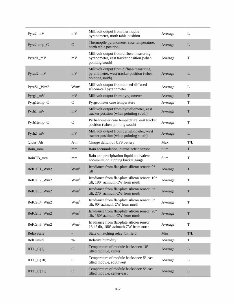
A-2
Pyra2_mV mV Millivolt output from thermopile
pyranometer, north table position Average L
Pyra2temp_C C Thermopile pyranometer case temperature,
north table position Average L
Pyrad1_mV mV
Millivolt output from diffuse-measuring
pyranometer, east tracker position (when
pointing south)
Average T
Pyrad2_mV mV
Millivolt output from diffuse-measuring
pyranometer, west tracker position (when
pointing south)
Average L
PyraS1_Wm2 W/m2 Millivolt output from domed-diffused
silicon-cell pyranometer Average L
Pyrg1_mV mV Millivolt output from pyrgeometer Average T
Pyrg1temp_C C Pyrgeometer case temperature Average T
Pyrh1_mV mV Millivolt output from pyrheliometer, east
tracker position (when pointing south) Average T
Pyrh1temp_C C Pyrheliometer case temperature, east tracker
position (when pointing south) Average T
Pyrh2_mV mV Millivolt output from pyrheliometer, west
tracker position (when pointing south) Average L
Qloss_Ah A·h Charge deficit of UPS battery Max T/L
Rain_mm mm Rain accumulation, piezoelectric sensor Sum T
RainTB_mm mm Rain and precipitation liquid equivalent
accumulation, tipping bucket gauge Sum T
RefCell1_Wm2 W/m2 Irradiance from flat-plate silicon sensor, 0°
tilt Average T
RefCell2_Wm2 W/m2 Irradiance from flat-plate silicon sensor, 10°
tilt, 180° azimuth CW from north Average T
RefCell3_Wm2 W/m2 Irradiance from flat-plate silicon sensor, 5°
tilt, 270° azimuth CW from north Average T
RefCell4_Wm2 W/m2 Irradiance from flat-plate silicon sensor, 5°
tilt, 90° azimuth CW from north Average T
RefCell5_Wm2 W/m2 Irradiance from flat-plate silicon sensor, 20°
tilt, 180° azimuth CW from north Average T
RefCell6_Wm2 W/m2 Irradiance from flat-plate silicon sensor,
18.4° tilt, 180° azimuth CW from north Average T
RelayState - State of latching relay, bit field Min T/L
RelHumid % Relative humidity Average T
RTD_C(1) C Temperature of module backsheet: 10°
tilted module, center Average L
RTD_C(10) C Temperature of module backsheet: 5° east
tilted module, southwest Average L
RTD_C(11) C Temperature of module backsheet: 5° east
tilted module, center-east Average L
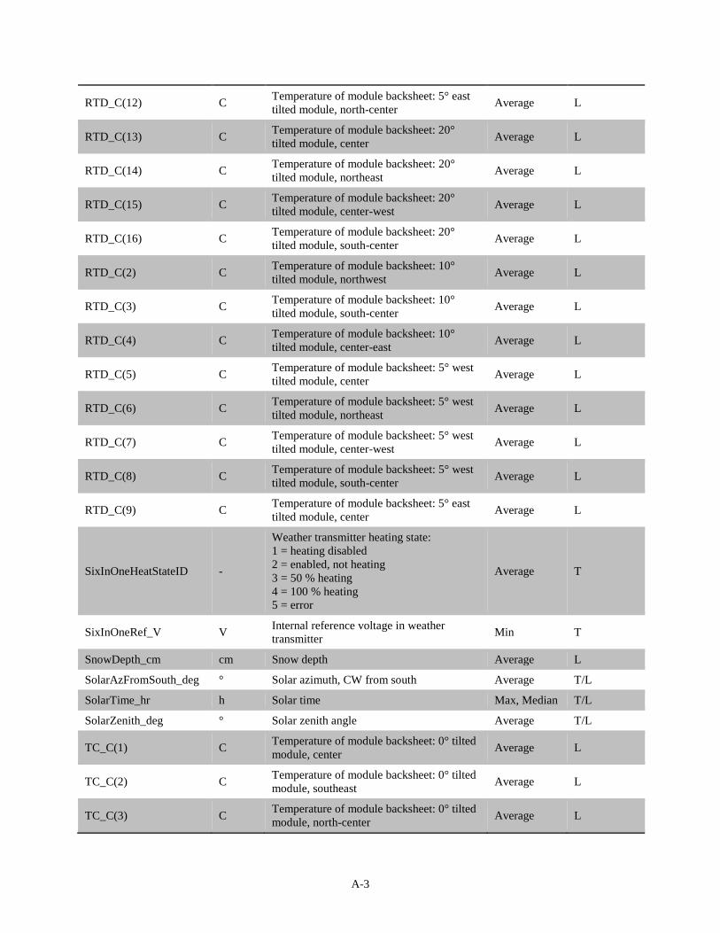
A-3
RTD_C(12) C Temperature of module backsheet: 5° east
tilted module, north-center Average L
RTD_C(13) C Temperature of module backsheet: 20°
tilted module, center Average L
RTD_C(14) C Temperature of module backsheet: 20°
tilted module, northeast Average L
RTD_C(15) C Temperature of module backsheet: 20°
tilted module, center-west Average L
RTD_C(16) C Temperature of module backsheet: 20°
tilted module, south-center Average L
RTD_C(2) C Temperature of module backsheet: 10°
tilted module, northwest Average L
RTD_C(3) C Temperature of module backsheet: 10°
tilted module, south-center Average L
RTD_C(4) C Temperature of module backsheet: 10°
tilted module, center-east Average L
RTD_C(5) C Temperature of module backsheet: 5° west
tilted module, center Average L
RTD_C(6) C Temperature of module backsheet: 5° west
tilted module, northeast Average L
RTD_C(7) C Temperature of module backsheet: 5° west
tilted module, center-west Average L
RTD_C(8) C Temperature of module backsheet: 5° west
tilted module, south-center Average L
RTD_C(9) C Temperature of module backsheet: 5° east
tilted module, center Average L
SixInOneHeatStateID -
Weather transmitter heating state:
1 = heating disabled
2 = enabled, not heating
3 = 50 % heating
4 = 100 % heating
5 = error
Average T
SixInOneRef_V V Internal reference voltage in weather
transmitter Min T
SnowDepth_cm cm Snow depth Average L
SolarAzFromSouth_deg ° Solar azimuth, CW from south Average T/L
SolarTime_hr h Solar time Max, Median T/L
SolarZenith_deg ° Solar zenith angle Average T/L
TC_C(1) C Temperature of module backsheet: 0° tilted
module, center Average L
TC_C(2) C Temperature of module backsheet: 0° tilted
module, southeast Average L
TC_C(3) C Temperature of module backsheet: 0° tilted
module, north-center Average L
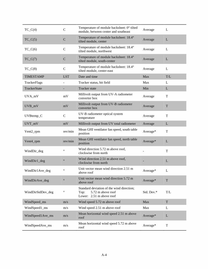
A-4
TC_C(4) C Temperature of module backsheet: 0° tilted
module, between center and southeast Average L
TC_C(5) C Temperature of module backsheet: 18.4°
tilted module, center Average L
TC_C(6) C Temperature of module backsheet: 18.4°
tilted module, northwest Average L
TC_C(7) C Temperature of module backsheet: 18.4°
tilted module, south-center Average L
TC_C(8) C Temperature of module backsheet: 18.4°
tilted module, center-east Average L
TIMESTAMP LST Date and time Max T/L
TrackerFlags - Tracker status, bit field Max L
TrackerState - Tracker state Min L
UVA_mV mV Millivolt output from UV-A radiometer
converter box Average T
UVB_mV mV Millivolt output from UV-B radiometer
converter box Average T
UVBtemp_C C UV-B radiometer optical system
temperature Average T
UVT_mV mV Millivolt output from UV total radiometer Average L
Vent2_rpm rev/min Mean GHI ventilator fan speed, south table
position Average* T
Vent4_rpm rev/min Mean GHI ventilator fan speed, north table
position Average* L
WindDir_deg ° Wind direction 5.72 m above roof,
clockwise from north - T
WindDir1_deg ° Wind direction 2.51 m above roof,
clockwise from north - L
WindDir1Ave_deg ° Unit vector mean wind direction 2.51 m
above roof Average* L
WindDirAve_deg ° Unit vector mean wind direction 5.72 m
above roof Average* T
WindDirStdDev_deg °
Standard deviation of the wind direction;
Top: 5.72 m above roof
Lower: 2.51 m above roof
Std. Dev.* T/L
WindSpeed_ms m/s Wind speed 5.72 m above roof Max T
WindSpeed1_ms m/s Wind speed 2.51 m above roof Max L
WindSpeed1Ave_ms m/s Mean horizontal wind speed 2.51 m above
roof Average* L
WindSpeedAve_ms m/s Mean horizontal wind speed 5.72 m above
roof Average* T
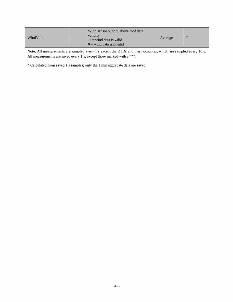
A-5
WindValid -
Wind sensor 5.72 m above roof data
validity
-1 = wind data is valid
0 = wind data is invalid
Average T
Note: All measurements are sampled every 1 s except the RTDs and thermocouples, which are sampled every 10 s.
All measurements are saved every 1 s, except those marked with a “*”.
* Calculated from saved 1 s samples; only the 1 min aggregate data are saved
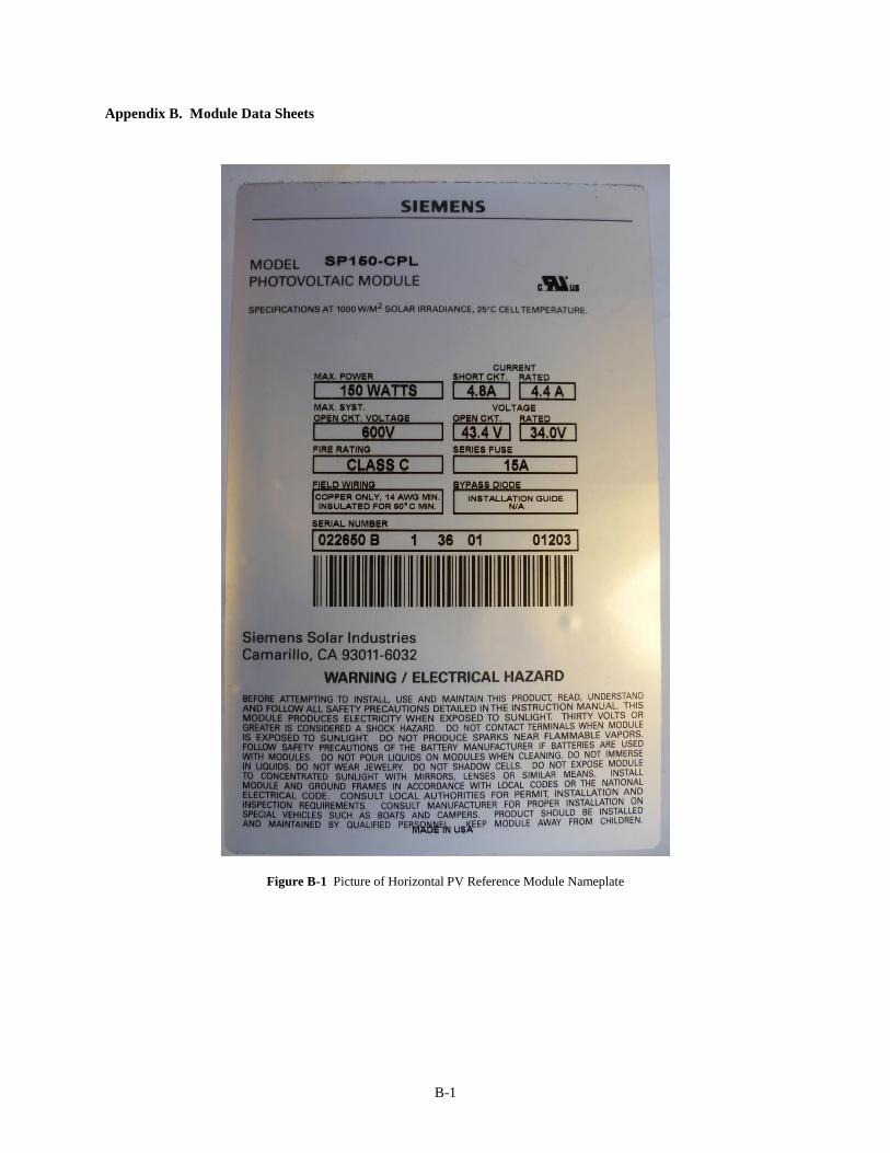
B-1
Appendix B. Module Data Sheets
Figure B-1 Picture of Horizontal PV Reference Module Nameplate
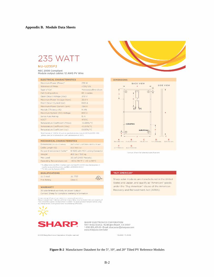
B-2
Appendix B. Module Data Sheets
Figure B-2 Manufacturer Datasheet for the 5°, 10°, and 20° Tilted PV Reference Modules
B-3
Appendix B. Module Data Sheets
Figure B-3 Manufacturer Datasheet for the 18.4° PV Reference Module


