NISP Toolbox Manual - Scilabforge.scilab.org/upload/nisp/files/nisp_toolbox_manual_v... ·...

NISP Toolbox Manual

Michael Baudin (INRIA)Jean-Marc Martinez (CEA)

Version 0.2January 2011

Abstract

This document is an introduction to the NISP module. We present the installation process of themodule in binary from ATOMS or from the sources. Then we present the configuration functionsand the randvar, setrandvar and polychaos classes. Several examples are provided for each class,which provides an overview of the use of NISP in practical situations. In the last section, wepresent an introduction to sensivity analysis and show how to use Scilab and the NISP modulein this context.

Contents

1 Introduction 31.1 The OPUS project . . . . . . . . . . . . . . . . . . . . . . . . . . . . . . . . . . . 31.2 The NISP library . . . . . . . . . . . . . . . . . . . . . . . . . . . . . . . . . . . . 31.3 The NISP module . . . . . . . . . . . . . . . . . . . . . . . . . . . . . . . . . . . . 4

2 Installation 92.1 Introduction . . . . . . . . . . . . . . . . . . . . . . . . . . . . . . . . . . . . . . . 92.2 Installing the toolbox from ATOMS . . . . . . . . . . . . . . . . . . . . . . . . . . 102.3 Installing the toolbox from the sources . . . . . . . . . . . . . . . . . . . . . . . . 11

3 Configuration functions 16

4 The randvar class 174.1 The distribution functions . . . . . . . . . . . . . . . . . . . . . . . . . . . . . . . 17

4.1.1 Overview . . . . . . . . . . . . . . . . . . . . . . . . . . . . . . . . . . . . 174.1.2 Parameters of the Log-normal distribution . . . . . . . . . . . . . . . . . . 184.1.3 Uniform random number generation . . . . . . . . . . . . . . . . . . . . . . 18

4.2 Methods . . . . . . . . . . . . . . . . . . . . . . . . . . . . . . . . . . . . . . . . . 194.2.1 Overview . . . . . . . . . . . . . . . . . . . . . . . . . . . . . . . . . . . . 194.2.2 The Oriented-Object system . . . . . . . . . . . . . . . . . . . . . . . . . . 19

4.3 Examples . . . . . . . . . . . . . . . . . . . . . . . . . . . . . . . . . . . . . . . . 214.3.1 A sample session . . . . . . . . . . . . . . . . . . . . . . . . . . . . . . . . 224.3.2 Variable transformations . . . . . . . . . . . . . . . . . . . . . . . . . . . . 22

5 The setrandvar class 275.1 Introduction . . . . . . . . . . . . . . . . . . . . . . . . . . . . . . . . . . . . . . . 275.2 Examples . . . . . . . . . . . . . . . . . . . . . . . . . . . . . . . . . . . . . . . . 27

5.2.1 A Monte-Carlo design with 2 variables . . . . . . . . . . . . . . . . . . . . 275.2.2 A Monte-Carlo design with 2 variables . . . . . . . . . . . . . . . . . . . . 315.2.3 A LHS design . . . . . . . . . . . . . . . . . . . . . . . . . . . . . . . . . . 335.2.4 A note on the LHS samplings . . . . . . . . . . . . . . . . . . . . . . . . . 375.2.5 Other types of DOEs . . . . . . . . . . . . . . . . . . . . . . . . . . . . . . 40

6 The polychaos class 446.1 Introduction . . . . . . . . . . . . . . . . . . . . . . . . . . . . . . . . . . . . . . . 446.2 Examples . . . . . . . . . . . . . . . . . . . . . . . . . . . . . . . . . . . . . . . . 44

6.2.1 Product of two random variables . . . . . . . . . . . . . . . . . . . . . . . 44

1

6.2.2 A note on performance . . . . . . . . . . . . . . . . . . . . . . . . . . . . . 496.2.3 The Ishigami test case . . . . . . . . . . . . . . . . . . . . . . . . . . . . . 51

7 An introduction to sensitivity analysis 557.1 Sensitivity analysis . . . . . . . . . . . . . . . . . . . . . . . . . . . . . . . . . . . 557.2 Standardized regression coefficients of affine models . . . . . . . . . . . . . . . . . 567.3 Link with the linear correlation coefficients . . . . . . . . . . . . . . . . . . . . . . 577.4 An example of affine model . . . . . . . . . . . . . . . . . . . . . . . . . . . . . . 587.5 Sensitivity analysis for nonlinear models . . . . . . . . . . . . . . . . . . . . . . . 617.6 The product of two variables . . . . . . . . . . . . . . . . . . . . . . . . . . . . . . 637.7 Sobol decomposition . . . . . . . . . . . . . . . . . . . . . . . . . . . . . . . . . . 707.8 Decomposition of the expectation . . . . . . . . . . . . . . . . . . . . . . . . . . . 737.9 Decomposition of the variance . . . . . . . . . . . . . . . . . . . . . . . . . . . . . 747.10 Higher order sensitivity indices . . . . . . . . . . . . . . . . . . . . . . . . . . . . 757.11 Total sensitivity indices . . . . . . . . . . . . . . . . . . . . . . . . . . . . . . . . . 777.12 Ishigami function . . . . . . . . . . . . . . . . . . . . . . . . . . . . . . . . . . . . 78

7.12.1 Elementary integration . . . . . . . . . . . . . . . . . . . . . . . . . . . . . 787.12.2 Expectation . . . . . . . . . . . . . . . . . . . . . . . . . . . . . . . . . . . 807.12.3 Variance . . . . . . . . . . . . . . . . . . . . . . . . . . . . . . . . . . . . . 817.12.4 Sobol decomposition . . . . . . . . . . . . . . . . . . . . . . . . . . . . . . 827.12.5 Summary of the results . . . . . . . . . . . . . . . . . . . . . . . . . . . . . 867.12.6 Numerical results . . . . . . . . . . . . . . . . . . . . . . . . . . . . . . . . 87

7.13 A straightforward approach . . . . . . . . . . . . . . . . . . . . . . . . . . . . . . 897.14 The Sobol method for sensitivity analysis . . . . . . . . . . . . . . . . . . . . . . . 907.15 The Ishigami function by the Sobol method . . . . . . . . . . . . . . . . . . . . . 947.16 Notes and references . . . . . . . . . . . . . . . . . . . . . . . . . . . . . . . . . . 97

8 Thanks 98

Bibliography 99

2

Chapter 1

Introduction

1.1 The OPUS project

The goal of this toolbox is to provide a tool to manage uncertainties in simulated models. Thistoolbox is based on the NISP library, where NISP stands for ”Non-Intrusive Spectral Projection”.This work has been realized in the context of the OPUS project,

http://opus-project.fr

”Open-Source Platform for Uncertainty treatments in Simulation”, funded by ANR, the french”Agence Nationale pour la Recherche”:

http://www.agence-nationale-recherche.fr

The toolbox is released under the Lesser General Public Licence (LGPL), as all components ofthe OPUS project.

This module was presented in the ”42Almes JournAl’es de Statistique, du 24 au 28 mai 2010”[3].

1.2 The NISP library

The NISP library is based on a set of 3 C++ classes so that it provides an object-orientedframework for uncertainty analysis. The Scilab toolbox provides a pseudo-object oriented interfaceto this library, so that the two approaches are consistent. The NISP library is release under theLGPL licence.

The NISP library provides three tools, which are detailed below.

• The ”randvar” class allows to manage random variables, specified by their distribution lawand their parameters. Once a random variable is created, one can generate random numbersfrom the associated law.

• The ”setrandvar” class allows to manage a collection of random variables. This collectionis associated with a sampling method, such as MonteCarlo, Sobol, Quadrature, etc... It ispossible to build the sample and to get it back so that the experiments can be performed.

3

http://opus-project.fr

http://www.agence-nationale-recherche.fr

• The ”polychaos” class allows to manage a polynomial representation of the simulated model.One such object must be associated with a set of experiments which have been performed.This set may be read from a data file. The object is linked with a collection of randomvariables. Then the coefficients of the polynomial can be computed by integration (quadra-ture). Once done, the mean, the variance and the Sobol indices can be directly computedfrom the coefficients.

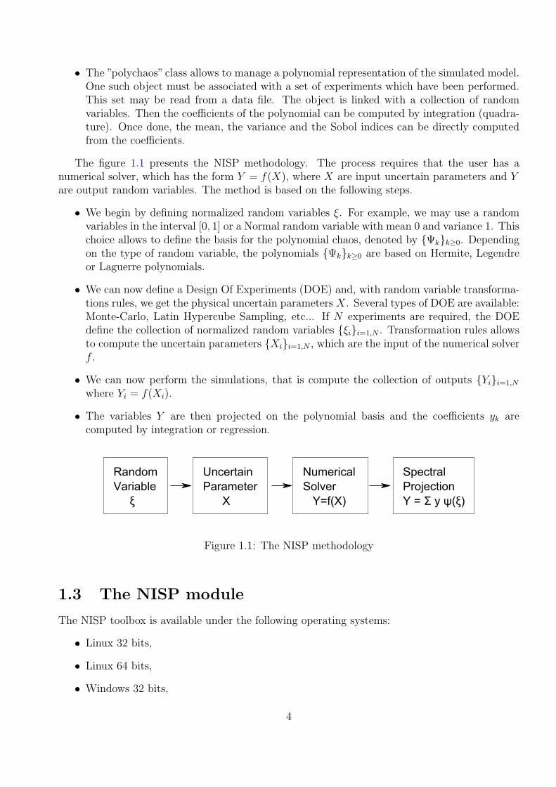
The figure 1.1 presents the NISP methodology. The process requires that the user has anumerical solver, which has the form Y = f(X), where X are input uncertain parameters and Yare output random variables. The method is based on the following steps.

• We begin by defining normalized random variables ξ. For example, we may use a randomvariables in the interval [0, 1] or a Normal random variable with mean 0 and variance 1. Thischoice allows to define the basis for the polynomial chaos, denoted by {Ψk}k≥0. Dependingon the type of random variable, the polynomials {Ψk}k≥0 are based on Hermite, Legendreor Laguerre polynomials.

• We can now define a Design Of Experiments (DOE) and, with random variable transforma-tions rules, we get the physical uncertain parameters X. Several types of DOE are available:Monte-Carlo, Latin Hypercube Sampling, etc... If N experiments are required, the DOEdefine the collection of normalized random variables {ξi}i=1,N . Transformation rules allowsto compute the uncertain parameters {Xi}i=1,N , which are the input of the numerical solverf .

• We can now perform the simulations, that is compute the collection of outputs {Yi}i=1,N

where Yi = f(Xi).

• The variables Y are then projected on the polynomial basis and the coefficients yk arecomputed by integration or regression.

RandomVariable ξ

UncertainParameter X

NumericalSolver Y=f(X)

SpectralProjectionY = Σ y ψ(ξ)

Figure 1.1: The NISP methodology

1.3 The NISP module

The NISP toolbox is available under the following operating systems:

• Linux 32 bits,

• Linux 64 bits,

• Windows 32 bits,

4

• Mac OS X.

The following list presents the features provided by the NISP toolbox.

• Manage various types of random variables:

– uniform,

– normal,

– exponential,

– log-normal.

• Generate random numbers from a given random variable,

• Transform an outcome from a given random variable into another,

• Manage various Design of Experiments for sets of random variables,

– Monte-Carlo,

– Sobol,

– Latin Hypercube Sampling,

– various samplings based on Smolyak designs.

• Manage polynomial chaos expansion and get specific outputs, including

– mean,

– variance,

– quantile,

– correlation,

– etc...

• Generate the C source code which computes the output of the polynomial chaos expansion.

This User’s Manual completes the online help provided with the toolbox, but does not replaceit. The goal of this document is to provide both a global overview of the toolbox and to give somedetails about its implementation. The detailed calling sequence of each function is provided bythe online help and will not be reproduced in this document. The inline help is presented in thefigure 1.2.

For example, in order to access to the help associated with the randvar class, we type thefollowing statements in the Scilab console.

help randvar

The previous statements opens the Help Browser and displays the helps page presented in figureSeveral demonstration scripts are provided with the toolbox and are presented in the figure

1.4. These demonstrations are available under the ”?” question mark in the menu of the Scilabconsole.

Finally, the unit tests provided with the toolbox cover all the features of the toolbox. Whenwe want to know how to use a particular feature and do not find the information, we can searchin the unit tests which often provide the answer.

5

Figure 1.2: The NISP inline help.

6

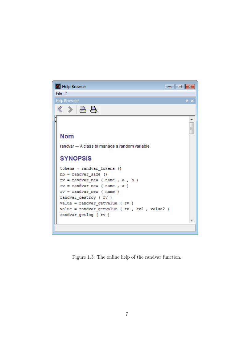
Figure 1.3: The online help of the randvar function.

7

Figure 1.4: Demonstrations provided with the NISP toolbox.

8

Chapter 2

Installation

In this section, we present the installation process for the toolbox. We present the steps whichare required to have a running version of the toolbox and presents the several checks which canbe performed before using the toolbox.

2.1 Introduction

There are two possible ways of installing the NISP toolbox in Scilab:

• use the ATOMS system and get a binary version of the toolbox,

• build the toolbox from the sources.

The next two sections present these two ways of using the toolbox.Before getting into the installation process, let us present some details of the the internal

components of the toolbox. The following list is an overview of the content of the directories:

• tbxnisp/demos : demonstration scripts

• tbxnisp/doc : the documentation

• tbxnisp/doc/usermanual : the LATEXsources of this manual

• tbxnisp/etc : startup and shutdow scripts for the toolbox

• tbxnisp/help : inline help pages

• tbxnisp/macros : Scilab macros files *.sci

• tbxnisp/sci gateway : the sources of the gateway

• tbxnisp/src : the sources of the NISP library

• tbxnisp/tests : tests

• tbxnisp/tests/nonreg tests : tests after some bug has been identified

• tbxnisp/tests/unit tests : unit tests

The current version is based on the NISP Library v2.1.

9

2.2 Installing the toolbox from ATOMS

The ATOMS component is the Scilab tool which allows to search, download, install and loadtoolboxes. ATOMS comes with Scilab v5.2. The Scilab-NISP toolbox has been packaged and isprovided mainly by the ATOMS component. The toolbox is provided in binary form, dependingon the user’s operating system. The Scilab-NISP toolbox is available for the following platforms:

• Windows 32 bits,

• Linux 32 bits, 64 bits,

• Mac OS X.

The ATOMS component allows to use a toolbox based on compiled source code, without havinga compiler installed in the system.

Installing the Scilab-NISP toolbox from ATOMS requires the following steps:

• atomsList(): prints the list of current toolboxes,

• atomsShow(): prints informations about a toolbox,

• atomsInstall(): installs a toolbox on the system,

• atomsLoad(): loads a toolbox.

Once installed and loaded, the toolbox will be available on the system from session to session, sothat there is no need to load the toolbox again: it will be available right from the start of thesession.

In the following Scilab session, we use the atomsList() function to print the list of all ATOMStoolboxes.

--> atomsList ()ANN_Toolbox - ANN Toolboxdde_toolbox - Dynamic Data Exchange client for Scilab

module_lycee - Scilab pour les lyc~Al’esNISP - Non Intrusive Spectral Projection

plotlib - "Matlab -like" Plotting library for Scilabscipad - Scipad 7.20

sndfile_toolbox - Read & write sound filesstixbox - Statistics toolbox for Scilab 5.2

In the following Scilab session, we use the atomsShow() function to print the details aboutthe NISP toolbox.

-->atomsShow ("NISP")Package : NISP

Title : NISPSummary : Non Intrusive Spectral ProjectionVersion : 2.1Depend : Category(ies) : Optimization

Maintainer(s) : Pierre Marechal <[email protected] >Michael Baudin <[email protected] >

10

Entity : CEA / DIGITEOWebSite : License : LGPL

Scilab Version : >= 5.2.0Status : Not installed

Description : This toolbox allows to approximate a given model ,which is associated with input random variables.This toolbox has been created in the context of theOPUS project :

http ://opus -project.fr/within the workpackage 2.1.1:

"Construction de m~Al’ta-mod~Alles"This project has received funding by Agence Nationalede la recherche :

http :// www.agence -nationale -recherche.fr/See in the help provided in the help/en_US directoryof the toolbox for more information about its use.Use cases are presented in the demos directory.

In the following Scilab session, we use the atomsInstall() function to download and installthe binary version of the toolbox corresponding to the current operating system.

-->atomsInstall ( "NISP" )ans =!NISP 2.1 allusers D:\ Programs\SC3623 ~1\ contrib\NISP \2.1 I !

The "allusers" option of the atomsInstall function can be used to install the toolbox for allthe users of this computer. We finally load the toolbox with the atomsLoad() function.

-->atomsLoad ("NISP")Start NISP Toolbox

Load gatewaysLoad helpLoad demos

ans =!NISP 2.1 D:\ Programs\SC3623 ~1\ contrib\NISP \2.1 !

Now that the toolbox is loaded, it will be automatically loaded at the next Scilab session.

2.3 Installing the toolbox from the sources

In this section, we present the steps which are required in order to install the toolbox from thesources.

In order to install the toolbox from the sources, a compiler is required to be installed on themachine. This toolbox can be used with Scilab v5.1 and Scilab v5.2. We suppose that the archivehas been unpacked in the ”tbxnisp” directory. The following is a short list of the steps which arerequired to setup the toolbox.

1. build the toolbox : run the tbxnisp/builder.sce script to create the binaries of the library,create the binaries for the gateway, generate the documentation

2. load the toolbox : run the tbxnisp/load.sce script to load all commands and setup thedocumentation

11

3. setup the startup configuration file of your Scilab system so that the toolbox is known atstartup (see below for details),

4. run the unit tests : run the tbxnisp/runtests.sce script to perform all unit tests and checkthat the toolbox is OK

5. run the demos : run the tbxnisp/rundemos.sce script to run all demonstration scripts andget a quick interactive overview of its features

The following script presents the messages which are generated when the builder of the toolboxis launched. The builder script performs the following steps:

• compile the NISP C++ library,

• compile the C++ gateway library (the glue between the library and Scilab),

• generate the Java help files from the .xml files,

• generate the loader script.

-->exec C:\ tbxnisp\builder.sce;Building sources ...

Generate a loader fileGenerate a MakefileRunning the MakefileCompilation of utils.cppCompilation of blas1_d.cppCompilation of dcdflib.cppCompilation of faure.cppCompilation of halton.cppCompilation of linpack_d.cppCompilation of niederreiter.cppCompilation of reversehalton.cppCompilation of sobol.cppBuilding shared library (be patient)Generate a cleaner fileGenerate a loader fileGenerate a MakefileRunning the MakefileCompilation of nisp_gc.cppCompilation of nisp_gva.cppCompilation of nisp_ind.cppCompilation of nisp_index.cppCompilation of nisp_inv.cppCompilation of nisp_math.cppCompilation of nisp_msg.cppCompilation of nisp_conf.cppCompilation of nisp_ort.cppCompilation of nisp_pc.cppCompilation of nisp_polyrule.cpp

12

Compilation of nisp_qua.cppCompilation of nisp_random.cppCompilation of nisp_smo.cppCompilation of nisp_util.cppCompilation of nisp_va.cppCompilation of nisp_smolyak.cppBuilding shared library (be patient)Generate a cleaner file

Building gateway ...Generate a gateway fileGenerate a loader fileGenerate a Makefile: MakelibRunning the makefileCompilation of nisp_gettoken.cppCompilation of nisp_gwsupport.cppCompilation of nisp_PolynomialChaos_map.cppCompilation of nisp_RandomVariable_map.cppCompilation of nisp_SetRandomVariable_map.cppCompilation of sci_nisp_startup.cppCompilation of sci_nisp_shutdown.cppCompilation of sci_nisp_verboselevelset.cppCompilation of sci_nisp_verboselevelget.cppCompilation of sci_nisp_initseed.cppCompilation of sci_randvar_new.cppCompilation of sci_randvar_destroy.cppCompilation of sci_randvar_size.cppCompilation of sci_randvar_tokens.cppCompilation of sci_randvar_getlog.cppCompilation of sci_randvar_getvalue.cppCompilation of sci_setrandvar_new.cppCompilation of sci_setrandvar_tokens.cppCompilation of sci_setrandvar_size.cppCompilation of sci_setrandvar_destroy.cppCompilation of sci_setrandvar_freememory.cppCompilation of sci_setrandvar_addrandvar.cppCompilation of sci_setrandvar_getlog.cppCompilation of sci_setrandvar_getdimension.cppCompilation of sci_setrandvar_getsize.cppCompilation of sci_setrandvar_getsample.cppCompilation of sci_setrandvar_setsample.cppCompilation of sci_setrandvar_save.cppCompilation of sci_setrandvar_buildsample.cppCompilation of sci_polychaos_new.cppCompilation of sci_polychaos_destroy.cppCompilation of sci_polychaos_tokens.cppCompilation of sci_polychaos_size.cppCompilation of sci_polychaos_setdegree.cppCompilation of sci_polychaos_getdegree.cppCompilation of sci_polychaos_freememory.cpp

13

Compilation of sci_polychaos_getdimoutput.cppCompilation of sci_polychaos_setdimoutput.cppCompilation of sci_polychaos_getsizetarget.cppCompilation of sci_polychaos_setsizetarget.cppCompilation of sci_polychaos_freememtarget.cppCompilation of sci_polychaos_settarget.cppCompilation of sci_polychaos_gettarget.cppCompilation of sci_polychaos_getdiminput.cppCompilation of sci_polychaos_getdimexp.cppCompilation of sci_polychaos_getlog.cppCompilation of sci_polychaos_computeexp.cppCompilation of sci_polychaos_getmean.cppCompilation of sci_polychaos_getvariance.cppCompilation of sci_polychaos_getcovariance.cppCompilation of sci_polychaos_getcorrelation.cppCompilation of sci_polychaos_getindexfirst.cppCompilation of sci_polychaos_getindextotal.cppCompilation of sci_polychaos_getmultind.cppCompilation of sci_polychaos_getgroupind.cppCompilation of sci_polychaos_setgroupempty.cppCompilation of sci_polychaos_getgroupinter.cppCompilation of sci_polychaos_getinvquantile.cppCompilation of sci_polychaos_buildsample.cppCompilation of sci_polychaos_getoutput.cppCompilation of sci_polychaos_getquantile.cppCompilation of sci_polychaos_getquantwilks.cppCompilation of sci_polychaos_getsample.cppCompilation of sci_polychaos_setgroupaddvar.cppCompilation of sci_polychaos_computeoutput.cppCompilation of sci_polychaos_setinput.cppCompilation of sci_polychaos_propagateinput.cppCompilation of sci_polychaos_getanova.cppCompilation of sci_polychaos_setanova.cppCompilation of sci_polychaos_getanovaord.cppCompilation of sci_polychaos_getanovaordco.cppCompilation of sci_polychaos_realisation.cppCompilation of sci_polychaos_save.cppCompilation of sci_polychaos_generatecode.cppBuilding shared library (be patient)Generate a cleaner file

Generating loader_gateway.sce...Building help ...Building the master document:

C:\ tbxnisp\help\en_USBuilding the manual file [javaHelp] inC:\ tbxnisp\help\en_US.(Please wait building ... this can take a while)Generating loader.sce...

The following script presents the messages which are generated when the loader of the toolbox

14

is launched. The loader script performs the following steps:

• load the gateway (and the NISP library),

• load the help,

• load the demo.

-->exec C:\ tbxnisp\loader.sce;Start NISP Toolbox

Load gatewaysLoad helpLoad demos

It is now necessary to setup your Scilab system so that the toolbox is loaded automaticallyat startup. The way to do this is to configure the Scilab startup configuration file. The directorywhere this file is located is stored in the Scilab variable SCIHOME. In the following Scilab session,we use Scilab v5.2.0-beta-1 in order to know the value of the SCIHOME global variable.

-->SCIHOMESCIHOME =C:\Users\baudin\AppData\Roaming\Scilab\scilab -5.2.0 -beta -1

On my Linux system, the Scilab 5.1 startup file is located in

/home/myname/.Scilab/scilab-5.1/.scilab.

On my Windows system, the Scilab 5.1 startup file is located in

C:/Users/myname/AppData/Roaming/Scilab/scilab-5.1/.scilab.

This file is a regular Scilab script which is automatically loaded at Scilab’s startup. If that filedoes not already exist, create it. Copy the following lines into the .scilab file and configure thepath to the toolboxes, stored in the SCILABTBX variable.

exec("C:\ tbxnisp\loader.sce");

The following script presents the messages which are generated when the unit tests script ofthe toolbox is launched.

-->exec C:\ tbxnisp\runtests.sce;Tests beginning the 2009/11/18 at 12:47:45

TMPDIR = C:\Users\baudin\AppData\Local\Temp\SCI_TMP_6372_001/004 - [tbxnisp] nisp .................. passed : ref created002/004 - [tbxnisp] polychaos1 ............ passed : ref created003/004 - [tbxnisp] randvar1 .............. passed : ref created004/004 - [tbxnisp] setrandvar1 ........... passed : ref created--------------------------------------------------------------Summarytests 4 - 100 %passed 0 - 0 %failed 0 - 0 %skipped 0 - 0 %length 3.84 sec--------------------------------------------------------------

Tests ending the 2009/11/18 at 12:47:48\ end{verbatim}

15

Chapter 3

Configuration functions

In this section, we present functions which allow to configure the NISP toolbox.The nisp_* functions allows to configure the global behaviour of the toolbox. These func-

tions allows to startup and shutdown the toolbox and initialize the seed of the random numbergenerator. They are presented in the figure 3.1.

nisp_startup () Starts up the NISP toolbox.nisp_shutdown () Shuts down the NISP toolbox.level = nisp_verboselevelget () Returns the current verbose level.nisp_verboselevelset ( level ) Sets the value of the verbose level.nisp_initseed ( seed ) Sets the seed of the uniform random number generator.nisp_destroyall Destroy all current objects.nisp_getpath Returns the path to the current module.nisp_printall Prints all current objects.

Figure 3.1: Outline of the configuration methods.

The user has no need to explicitely call the nisp_startup () and nisp_shutdown () func-tions. Indeed, these functions are called automatically by the etc/NISP.start and etc/NISP.quitscripts, located in the toolbox directory structure.

The nisp_initseed ( seed ) is especially useful when we want to have reproductible re-sults. It allows to set the seed of the generator at a particular value, so that the sequence ofuniform pseudo-random numbers is deterministic. When the toolbox is started up, the seed isautomatically set to 0, which allows to get the same results from session to session.

16

Chapter 4

The randvar class

In this section, we present the randvar class, which allows to define a random variable, and togenerate random numbers from a given distribution function.

4.1 The distribution functions

In this section, we present the distribution functions provided by the randvar class. We especiallypresent the Log-normal distribution function.

4.1.1 Overview

The table 4.1 gives the list of distribution functions which are available with the randvar class[7].

Each distribution functions have zero, one or two parameters. One random variable can bespecified by giving explicitely its parameters or by using default parameters. The parameters forall distribution function are presented in the figure 4.2, which also presents the conditions whichmust be satisfied by the parameters.

Name f(x) E(X) V (X)

”Normale” 12σ√

2πexp

(− 1

2(x−µ)2

σ2

)µ σ2

”Uniforme”{

1b−a , if x ∈ [a, b[0 if x /∈ [a, b[

b+a2

(b−a)212

”Exponentielle”{λ exp (−λx) , if x > 00 if x ≤ 0

1λ

1λ2

”LogNormale”

{1

σx√

2πexp

(− 1

2(ln(x)−µ)2

σ2

), if x > 0

0 if x ≤ 0exp

(µ+ 1

2σ2) (

exp(σ2)− 1)exp

(2µ+ σ2

)”LogUniforme”

{ 1x

1ln(b)−ln(a) , if x ∈ [a, b[

0 if x /∈ [a, b[b−a

ln(b)−ln(a)12

b2−a2

ln(b)−ln(a) − E(x)

Figure 4.1: Distributions functions of the randvar class. – The expected value is denoted byE(X) and the variance is denoted by V (X).

17

Name Parameter #1 : a Parameter #2 : b Conditions”Normale” µ = 0. σ = 1. σ > 0”Uniforme” a = 0. b = 1. a < b”Exponentielle” λ = 1. - -”LogNormale” µ′ = 0.1 σ = 1.0 µ′, σ > 0”LogUniforme” a = 0.1 b = 1.0 a, b > 0, a < b

Figure 4.2: Default parameters for distributions functions.

4.1.2 Parameters of the Log-normal distribution

A log-normal distribution is a probability distribution of a random variable whose logarithm isnormally distributed. If X is a random variable with a normal distribution, then Y = exp(X)has a log-normal distribution.

For the ”LogNormale” law, the distribution function is usually defined by the expected valueµ and the standard deviation σ of the underlying Normal random variable. But, when we createa LogNormale randvar, the parameters to pass to the constructor are the expected value of theLogNormal random variable E(X) and the standard deviation of the underlying Normale randomvariable σ. The expected value and the variance of the Log Normal law are given by

E(X) = exp

(µ+

1

2σ2

)(4.1)

V (X) =(exp(σ2)− 1

)exp

(2µ+ σ2

). (4.2)

In the figure 4.2, we have µ′ = E(X).It is possible to invert these formulas, in the situation where the given parameters are the

expected value and the variance of the Log Normal random variable. We can invert completelythe previous equations and get

µ = ln(E(X))− 1

2ln

(1 +

V (X)

E(X)2

)(4.3)

σ2 = ln

(1 +

V (X)

E(X)2

). (4.4)

In particular, the expected value µ of with the Normal random variable satisfies the equation

µ = ln(E(X))− σ2. (4.5)

4.1.3 Uniform random number generation

In this section, we present the generation of uniform random numbers.The goal of this section is to warn users about a current limitation of the library. Indeed, the

random number generator is based on the compiler, so that its quality cannot be guaranted.The Uniforme law is associated with the parameters a, b ∈ R with a < b. It produces real

values uniform in the interval [a, b].To compute the uniform random number X in the interval [a, b], a uniform random number

in the interval [0, 1] is generated and then scaled with

X = a+ (b− a)X. (4.6)

18

Let us now analyse how the uniform random number X ∈ [0, 1] is computed. The uniformrandom generator is based on the C function rand, which returns an integer n in the interval[0, RAND MAX[. The value of the RAND MAX variable is defined in the file stdlib.h and iscompiler-dependent. For example, with the Visual Studio C++ 2008 compiler, the value is

RAND MAX = 215 − 1 = 32767. (4.7)

A uniform value X in the range [0, 1[ is computed from

X =n

N, (4.8)

where N = RAND MAX and n ∈ [0, RAND MAX[.

4.2 Methods

In this section, we give an overview of the methods which are available in the randvar class.

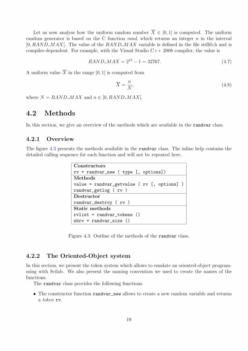
4.2.1 Overview

The figure 4.3 presents the methods available in the randvar class. The inline help contains thedetailed calling sequence for each function and will not be repeated here.

Constructorsrv = randvar_new ( type [, options])

Methodsvalue = randvar_getvalue ( rv [, options] )

randvar_getlog ( rv )

Destructorrandvar_destroy ( rv )

Static methodsrvlist = randvar_tokens ()

nbrv = randvar_size ()

Figure 4.3: Outline of the methods of the randvar class.

4.2.2 The Oriented-Object system

In this section, we present the token system which allows to emulate an oriented-object program-ming with Scilab. We also present the naming convention we used to create the names of thefunctions.

The randvar class provides the following functions.

• The constructor function randvar_new allows to create a new random variable and returnsa token rv.

19

• The method randvar_getvalue takes the token rv as its first argument. In fact, all methodstakes as their first argument the object on which they apply.

• The destructor randvar_destroy allows to delete the current object from the memory ofthe library.

• The static methods randvar_tokens and randvar_size allows to quiery the current objectwhich are in use. More specifically, the randvar_size function returns the number of currentrandvar objects and the randvar_tokens returns the list of current randvar objects.

In the following Scilab sessions, we present these ideas with practical uses of the toolbox.Assume that we start Scilab and that the toolbox is automatically loaded. At startup, there

are no objects, so that the randvar_size function returns 0 and the randvar_tokens functionreturns an empty matrix.

-->nb = randvar_size ()nb =

0.-->tokenmatrix = randvar_tokens ()tokenmatrix =

[]

We now create 3 new random variables, based on the Uniform distribution function. We storethe tokens in the variables vu1, vu2 and vu3. These variables are regular Scilab double precisionfloating point numbers. Each value is a token which represents a random variable stored in thetoolbox memory space.

-->vu1 = randvar_new("Uniforme")vu1 =

0.-->vu2 = randvar_new("Uniforme")vu2 =


2.

There are now 3 objects in current use, as indicated by the following statements. Thetokenmatrix is a row matrix containing regular double precision floating point numbers.



0. 1. 2.

We assume that we have now made our job with the random variables, so that it is timeto destroy the random variables. We call the randvar_destroy functions, which destroys thevariables.

-->randvar_destroy(vu1);-->randvar_destroy(vu2);-->randvar_destroy(vu3);

20

We can finally check that there are no random variables left in the memory space.



[]

Scilab is a wonderful tool to experiment algorithms and make simulations. It happens some-times that we are managing many variables at the same time and it may happen that, at somepoint, we are lost. The static methods provides tools to be able to recover from such a situationwithout closing our Scilab session.

In the following session, we create two random variables.

-->vu1 = randvar_new("Uniforme")vu1 =


4.

Assume now that we have lost the token associated with the variable vu2. We can easily simulatethis situation, by using the clear, which destroys a variable from Scilab’s memory space.

-->clear vu2-->randvar_getvalue(vu2)

!--error 4Undefined variable: vu2

It is now impossible to generate values from the variable vu2. Moreover, it may be difficult toknow exactly what went wrong and what exact variable is lost. At any time, we can use therandvar_tokens function in order to get the list of current variables. Deleting these variablesallows to clean the memory space properly, without memory loss.

-->randvar_tokens ()ans =

3. 4.-->randvar_destroy (3)ans =

3.-->randvar_destroy (4)ans =

4.-->randvar_tokens ()ans =

[]

4.3 Examples

In this section, we present to examples of use of the randvar class. The first example presentsthe simulation of a Normal random variable and the generation of 1000 random variables. The

21

second example presents the transformation of a Uniform outcome into a LogUniform outcome.

4.3.1 A sample session

We present a sample Scilab session, where the randvar class is used to generate samples from theNormale law.

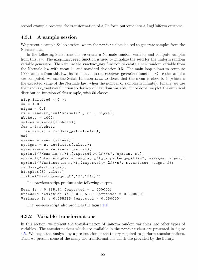
In the following Scilab session, we create a Normale random variable and compute samplesfrom this law. The nisp_initseed function is used to initialize the seed for the uniform randomvariable generator. Then we use the randvar_new function to create a new random variable fromthe Normale law with mean 1. and standard deviation 0.5. The main loop allows to compute1000 samples from this law, based on calls to the randvar_getvalue function. Once the samplesare computed, we use the Scilab function mean to check that the mean is close to 1 (which isthe expected value of the Normale law, when the number of samples is infinite). Finally, we usethe randvar_destroy function to destroy our random variable. Once done, we plot the empiricaldistribution function of this sample, with 50 classes.

nisp_initseed ( 0 );mu = 1.0;sigma = 0.5;rv = randvar_new("Normale" , mu , sigma);nbshots = 1000;values = zeros(nbshots );for i=1: nbshots

values(i) = randvar_getvalue(rv);endmymean = mean (values );mysigma = st_deviation(values );myvariance = variance (values );mprintf("Mean is : %f (expected = %f)\n", mymean , mu);mprintf("Standard deviation is : %f (expected = %f)\n", mysigma , sigma );mprintf("Variance is : %f (expected = %f)\n", myvariance , sigma ^2);randvar_destroy(rv);histplot (50, values)xtitle("Histogram of X","X","P(x)")

The previous script produces the following output.

Mean is : 0.988194 (expected = 1.000000)Standard deviation is : 0.505186 (expected = 0.500000)Variance is : 0.255213 (expected = 0.250000)

The previous script also produces the figure 4.4.

4.3.2 Variable transformations

In this section, we present the transformation of uniform random variables into other types ofvariables. The transformations which are available in the randvar class are presented in figure4.5. We begin the analysis by a presentation of the theory required to perform transformations.Then we present some of the many the transformations which are provided by the library.

22

0.0

0.1

0.2

0.3

0.4

0.5

0.6

0.7

0.8

0.9

-1.0 -0.5 0.0 0.5 1.0 1.5 2.0 2.5 3.0

Histogram of X

X

P(x

)

Figure 4.4: The histogram of a Normal random variable with 1000 samples.

Source TargetNormale

NormaleUniformeExponentielleLogNormaleLogUniforme

Source TargetLogNormale

NormaleUniformeExponentielleLogNormaleLogUniforme

Source TargetUniforme

UniformeNormaleExponentielleLogNormaleLogUniforme

Source TargetLogUniforme

UniformeNormaleExponentielleLogNormaleLogUniforme

Source TargetExponentielle

Exponentielle

Figure 4.5: Variable transformations available in the randvar class.

23

We now present some additionnal details for the function randvar_getvalue ( rv , rv2 ,

value2 ). This method allows to transform a random variable sample from one law to another.The statement

value = randvar_getvalue ( rv , rv2 , value2 )

returns a random value from the distribution function of the random variable rv by transformationof value2 from the distribution function of random variable rv2.

In the following session, we transform a uniform random variable sample into a LogUniformvariable sample. We begin to create a random variable rv from a LogUniform law and parametersa = 10, b = 20. Then we create a second random variable rv2 from a Uniforme law and parametersa = 2, b = 3. The main loop is based on the transformation of a sample computed from rv2 intoa sample from rv. The mean allows to check that the transformed samples have an mean valuewhich corresponds to the random variable rv.

nisp_initseed ( 0 );a = 10.0;b = 20.0;rv = randvar_new ( "LogUniforme" , a , b );rv2 = randvar_new ( "Uniforme" , 2 , 3 );nbshots = 1000;valuesLou = zeros(nbshots );for i=1: nbshots

valuesUni(i) = randvar_getvalue( rv2 );valuesLou(i) = randvar_getvalue( rv , rv2 , valuesUni(i) );

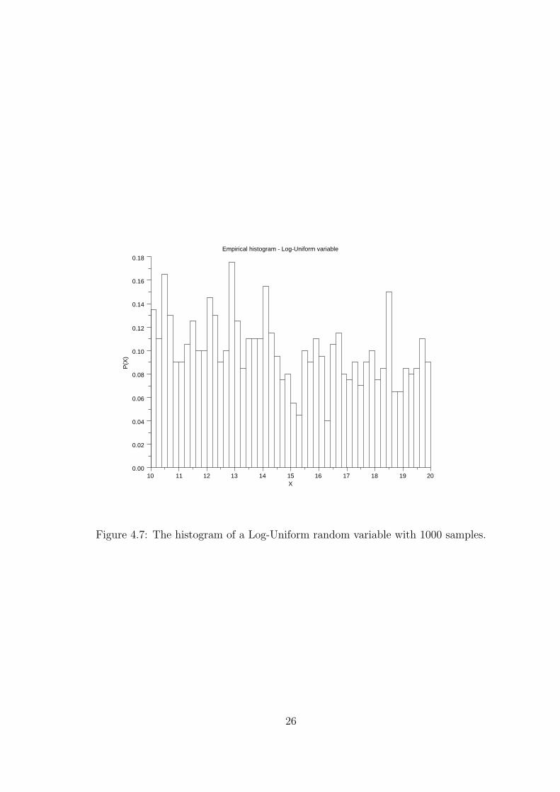
endcomputed = mean (valuesLou );mu = (b-a)/(log(b)-log(a));expected = mu;mprintf("Expectation=%.5f (expected=%.5f)\n",computed ,expected );//scf();histplot (50, valuesUni );xtitle("Empirical histogram - Uniform variable","X","P(X)");scf();histplot (50, valuesLou );xtitle("Empirical histogram - Log -Uniform variable","X","P(X)");randvar_destroy(rv);randvar_destroy(rv2);


Expectation =14.63075 (expected =14.42695)

The previous script also produces the figures 4.6 and 4.7.The transformation depends on the mother random variable rv1 and on the daughter ran-

dom variable rv. Specific transformations are provided for all many combinations of the twodistribution functions. These transformations will be analysed in the next sections.

24

0.0

0.2

0.4

0.6

0.8

1.0

1.2

1.4

1.6

2.0 2.1 2.2 2.3 2.4 2.5 2.6 2.7 2.8 2.9 3.0

Empirical histogram - Uniform variable

X

P(X

)

Figure 4.6: The histogram of a Uniform random variable with 1000 samples.

25

0.00

0.02

0.04

0.06

0.08

0.10

0.12

0.14

0.16

0.18

10 11 12 13 14 15 16 17 18 19 20

Empirical histogram - Log-Uniform variable

X

P(X

)

Figure 4.7: The histogram of a Log-Uniform random variable with 1000 samples.

26

Chapter 5

The setrandvar class

In this chapter, we presen the setrandvar class. The first section gives a brief outline of thefeatures of this class and the second section present several examples.

5.1 Introduction

The setrandvar class allows to manage a collection of random variables and to build a DesignOf Experiments (DOE). Several types of DOE are provided:

• Monte-Carlo,

• Latin Hypercube Sampling,

• Smolyak.

Once a DOE is created, we can retrieve the information experiment by experiment or the wholematrix of experiments. This last feature allows to benefit from the fact that Scilab can nativelymanage matrices, so that we do not have to perform loops to manage the complete DOE. Hence,good performances can be observed, even if the language still is interpreted.

The figure 5.1 presents the methods available in the setrandvar class. A complete descriptionof the input and output arguments of each function is available in the inline help and will not berepeated here.

More informations about the Oriented Object system used in this toolbox can be found in thesection 4.2.2.

5.2 Examples

In this section, we present examples of use of the setrandvar class. In the first example, wepresent a Scilab session where we create a Latin Hypercube Sampling. In the second part, wepresent various types of DOE which can be generated with this class.

5.2.1 A Monte-Carlo design with 2 variables

In the following example, we build a Monte-Carlo design of experiments, with 2 input randomvariables. The first variable is associated with a Normal distribution function and the second

27

Constructorssrv = setrandvar_new ( )

srv = setrandvar_new ( n )

srv = setrandvar_new ( file )

Methodssetrandvar_setsample ( srv , name , np )

setrandvar_setsample ( srv , k , i , value )

setrandvar_setsample ( srv , k , value )

setrandvar_setsample ( srv , value )

setrandvar_save ( srv , file )

np = setrandvar_getsize ( srv )

sample = setrandvar_getsample ( srv , k , i )

sample = setrandvar_getsample ( srv , k )

sample = setrandvar_getsample ( srv )

setrandvar_getlog ( srv )

nx = setrandvar_getdimension ( srv )

setrandvar_freememory ( srv )

setrandvar_buildsample ( srv , srv2 )

setrandvar_buildsample ( srv , name , np )

setrandvar_buildsample ( srv , name , np , ne )

setrandvar_addrandvar ( srv , rv )

Destructorsetrandvar_destroy ( srv )

Static methodstokenmatrix = setrandvar_tokens ()

nb = setrandvar_size ()

Figure 5.1: Outline of the methods of the setrandvar class

28

variable is associated with a Uniform distribution function. The simulation is based on 1000experiments.

The function nisp_initseed is used to set the value of the seed to zero, so that the re-sults can be reproduced. The setrandvar_new function is used to create a new set of ran-dom variables. Then we create two new random variables with the randvar_new function.These two variables are added to the set with the setrandvar_addrandvar function. Thesetrandvar_buildsample allows to build the design of experiments, which can be retrievedas matrix with the setrandvar_getsample function. The sampling matrix has np rows and 2columns (one for each input variable).

nisp_initseed (0);rvu1 = randvar_new("Normale" ,1,3);rvu2 = randvar_new("Uniforme" ,2,3);//srvu = setrandvar_new ();setrandvar_addrandvar ( srvu , rvu1);setrandvar_addrandvar ( srvu , rvu2);//np = 5000;setrandvar_buildsample(srvu , "MonteCarlo",np);sampling = setrandvar_getsample(srvu);// Check sampling of random variable #1mean(sampling (:,1)) // Expectation : 1// Check sampling of random variable #2mean(sampling (:,2)) // Expectation : 2.5//scf();histplot (50, sampling (: ,1));xtitle("Empirical histogram of X1");scf();histplot (50, sampling (: ,2));xtitle("Empirical histogram of X2");//// Clean -upsetrandvar_destroy(srvu);randvar_destroy(rvu1);randvar_destroy(rvu2);


-->mean(sampling (:,1)) // Expectation : 1ans =

1.0064346-->mean(sampling (:,2)) // Expectation : 2.5ans =

2.5030984

The prevous script also produces the figures 5.2 and 5.3.We may now want to add the exact distribution to these histograms and compare. The Normal

distribution function is not provided by Scilab, but is provided by the Stixbox module. Indeed,the dnorm function of the Stixbox module computes the Normal probability distribution function.

29

0.00

0.05

0.10

-15 -10 -5 0 5 10 15

Empirical histogram of X1

Figure 5.2: Monte-Carlo Sampling - Normal random variable.

0.0

0.5

1.0

2.0 2.1 2.2 2.3 2.4 2.5 2.6 2.7 2.8 2.9 3.0


Figure 5.3: Monte-Carlo Sampling - Uniform random variable.

30

In order to install this module, we can run the atomsInstall function, as in the following script.

atomsInstall("stixbox")

The following script compares the empirical and theoretical distributions.

scf();histplot (50, sampling (: ,1));xtitle("Empirical histogram of X1");x=linspace ( -15 ,15 ,1000);y = dnorm(x,1,3);plot(x,y,"r-")legend (["Empirical","Exact"]);

The previous script produces the figure 5.4.

EmpiricalExact

0.00

0.05

0.10

-15 -10 -5 0 5 10 15

Figure 5.4: Monte-Carlo Sampling - Histogram and exact distribution functions for the firstvariable.

The following script performs the same comparison for the second variable.

scf();histplot (50, sampling (: ,2));xtitle("Empirical histogram of X2");x=linspace (2 ,3 ,1000);y=ones (1000 ,1);plot(x,y,"r-");


5.2.2 A Monte-Carlo design with 2 variables

In this section, we create a Monte-Carlo design with 2 variables.We are going to use the exponential distribution function, which is not defined in Scilab.

The following exppdf function computes the probability distribution function of the exponentialdistribution function.

31

0.0

0.5

1.0

2.0 2.1 2.2 2.3 2.4 2.5 2.6 2.7 2.8 2.9 3.0


Figure 5.5: Monte-Carlo Sampling - Histogram and exact distribution functions for the secondvariable.

function p = exppdf ( x , lambda )p = lambda .*exp(-lambda .*x)

endfunction

The following script creates a Monte-Carlo sampling where the first variable is Normal andthe second variable is Exponential. Then we compare the empirical histogram and the exactdistribution function. We use the dnorm function defined in the Stixbox module.

nisp_initseed ( 0 );rv1 = randvar_new("Normale" ,1.0 ,0.5);rv2 = randvar_new("Exponentielle" ,5.);// Definition d’un groupe de variables aleatoiressrv = setrandvar_new ( );setrandvar_addrandvar ( srv , rv1 );setrandvar_addrandvar ( srv , rv2 );np = 1000;setrandvar_buildsample ( srv , "MonteCarlo" , np );//sampling = setrandvar_getsample ( srv );// Check sampling of random variable #1mean(sampling (:,1)), variance(sampling (:,1))// Check sampling of random variable #2min(sampling (:,2)), max(sampling (:,2))// Plotscf();histplot (40, sampling (:,1))x = linspace (-1,3,1000)’;p = dnorm(x,1 ,0.5);plot(x,p,"r-")

32

xtitle("Empirical histogram of X1","X","P(X)");legend (["Empirical","Exact"]);scf();histplot (40, sampling (:,2))x = linspace (0,2 ,1000)’;p = exppdf ( x , 5 );plot(x,p,"r-")xtitle("Empirical histogram of X2","X","P(X)");legend (["Empirical","Exact"]);// Clean -upsetrandvar_destroy(srv);randvar_destroy(rv1);randvar_destroy(rv2);

The previous script produces the figures 5.6 and 5.7.

EmpiricalExact

0.0

0.1

0.2

0.3

0.4

0.5

0.6

0.7

0.8

0.9

1.0

-1.0 -0.5 0.0 0.5 1.0 1.5 2.0 2.5 3.0 3.5


X

P(X

)

Figure 5.6: Monte-Carlo Sampling - Histogram and exact distribution functions for the firstvariable.

5.2.3 A LHS design

In this section, we present the creation of a Latin Hypercube Sampling. In our example, the DOEis based on two random variables, the first being Normal with mean 1.0 and standard deviation0.5 and the second being Uniform in the interval [2, 3].

We begin by defining two random variables with the randvar_new function.

vu1 = randvar_new("Normale" ,1.0 ,0.5);vu2 = randvar_new("Uniforme" ,2.0 ,3.0);

Then, we create a collection of random variables with the setrandvar_new function whichcreates here an empty collection of random variables. Then we add the two random variables tothe collection.

33

EmpiricalExact

0.0

0.5

1.0

1.5

2.0

2.5

3.0

3.5

4.0

4.5

5.0

0.0 0.2 0.4 0.6 0.8 1.0 1.2 1.4 1.6 1.8 2.0


X

P(X

)

Figure 5.7: Monte-Carlo Sampling - Histogram and exact distribution functions for the secondvariable.

srv = setrandvar_new ( );setrandvar_addrandvar ( srv , vu1 );setrandvar_addrandvar ( srv , vu2 );

We can now build the DOE so that it is a LHS sampling with 1000 experiments.

setrandvar_buildsample ( srv , "Lhs" , 1000 );

At this point, the DOE is stored in the memory space of the NISP library, but we do not havea direct access to it. We now call the setrandvar_getsample function and store that DOE intothe sampling matrix.

sampling = setrandvar_getsample ( srv );

The sampling matrix has 1000 rows, corresponding to each experiment, and 2 columns, cor-responding to each input random variable.

The following script allows to plot the sampling, which is is presented in figure 5.8.

my_handle = scf();clf(my_handle ,"reset");plot(sampling (:,1), sampling (: ,2));my_handle.children.children.children.line_mode = "off";my_handle.children.children.children.mark_mode = "on";my_handle.children.children.children.mark_size = 2;my_handle.children.title.text = "Latin Hypercube Sampling";my_handle.children.x_label.text = "Variable #1 : Normale ,1.0 ,0.5";my_handle.children.y_label.text = "Variable #2 : Uniforme ,2.0 ,3.0";

The following script allows to plot the histogram of the two variables, which are presented infigures 5.9 and 5.10.

// Plot Var #1

34

Figure 5.8: Latin Hypercube Sampling - The first variable is Normal, the second variable isUniform.

35

my_handle = scf();clf(my_handle ,"reset");histplot ( 50 , sampling (:,1))my_handle.children.title.text = "Variable #1 : Normale ,1.0 ,0.5";// Plot Var #2my_handle = scf();clf(my_handle ,"reset");histplot ( 50 , sampling (:,2))my_handle.children.title.text = "Variable #2 : Uniforme ,2.0 ,3.0";

2.52.01.51.00.50.0-0.5-1.0

0.8

0.7

0.6

0.5

0.4

0.3

0.2

0.1

0.03.0

Variable #1 : Normale,1.0,0.5

Figure 5.9: Latin Hypercube Sampling - Normal random variable.

We can use the mean and variance on each random variable and check that the expectedresult is computed. We insist on the fact that the mean and variance functions are not providedby the NISP library: these are pre-defined functions which are available in the Scilab library. Thatmeans that any Scilab function can be now used to process the data generated by the toolbox.

for ivar = 1:2m = mean(sampling(:,ivar))mprintf("Variable #%d, Mean : %f\n",ivar ,m)v = variance(sampling(:,ivar))mprintf("Variable #%d, Variance : %f\n",ivar ,v)

end


Variable #1, Mean : 1.000000Variable #1, Variance : 0.249925Variable #2, Mean : 2.500000Variable #2, Variance : 0.083417

Our numerical simulation is now finished, but we must destroy the objects so that the memorymanaged by the toolbox is deleted.

36

2.92.82.72.62.52.42.32.22.12.0

1.2

1.0

0.8

0.6

0.4

0.2

0.03.0

Variable #2 : Uniforme,2.0,3.0

Figure 5.10: Latin Hypercube Sampling - Uniform random variable.

randvar_destroy(vu1)randvar_destroy(vu2)setrandvar_destroy(srv)

5.2.4 A note on the LHS samplings

We emphasize that the LHS sampling which is provided by the setrandvar_buildsample functionis so that the points are centered within their cells.

In the following script, we create a LHS sampling with 10 points.

srv = setrandvar_new (2);np = 10;setrandvar_buildsample ( srv , "Lhs" , np );sampling = setrandvar_getsample ( srv );scf();plot(sampling (:,1), sampling (:,2),"bo");xtitle("LHS Design","X1","X2");// Add the cutscut = linspace ( 0 , 1 , np + 1 );for i = 1 : np + 1

plot( [cut(i) cut(i)] , [0 1] , "-" )endfor i = 1 : np + 1

plot( [0 1] , [cut(i) cut(i)] , "-" )endsetrandvar_destroy ( srv )

The previous script produces the figure 5.11.The ”LhsMaxMin” sampling provided by the setrandvar_buildsample function tries to max-

imize the minimum distance between the points in the sampling. The ntry parameter is the

37

0.0

0.1

0.2

0.3

0.4

0.5

0.6

0.7

0.8

0.9

1.0

0.0 0.1 0.2 0.3 0.4 0.5 0.6 0.7 0.8 0.9 1.0

LHS Design

X1

X2

Figure 5.11: Latin Hypercube Sampling - Computed with setrandvar_buildsample and the”Lhs” option.

number of random points generated before the best is accepted in the sampling.

np = 10;ntry = 100;setrandvar_buildsample ( srv , "LhsMaxMin" , np , ntry );sampling = setrandvar_getsample ( srv );

The previous script produces the figure 5.12.On the other hand, the nisp_buildlhs function produces a more classical LHS sampling,

where the points are randomly picked within their cells.

n = 5;s = 2;sampling = nisp_buildlhs ( s , n );scf();plot ( sampling (:,1) , sampling (:,2) , "bo" );// Add the cutscut = linspace ( 0 , 1 , n + 1 );for i = 1 : n + 1plot( [cut(i) cut(i)] , [0 1] , "-" )endfor i = 1 : n + 1plot( [0 1] , [cut(i) cut(i)] , "-" )end


38

0.0

0.1

0.2

0.3

0.4

0.5

0.6

0.7

0.8

0.9

1.0

0.0 0.1 0.2 0.3 0.4 0.5 0.6 0.7 0.8 0.9 1.0

LHS Max Min Design

X1

X2

Figure 5.12: Latin Hypercube Sampling - Computed with setrandvar_buildsample and the”LhsMaxMin” option.

0.0

0.1

0.2

0.3

0.4

0.5

0.6

0.7

0.8

0.9

1.0

0.0 0.1 0.2 0.3 0.4 0.5 0.6 0.7 0.8 0.9 1.0

Figure 5.13: Latin Hypercube Sampling - Computed with nisp_buildlhs.

39

5.2.5 Other types of DOEs

The following Scilab session allows to generate a Monte-Carlo sampling with two uniform variablesin the interval [−1, 1]. The figure 5.14 presents this sampling and the figures 5.15 and 5.16 presentthe histograms of the two uniform random variables.

vu1 = randvar_new("Uniforme" ,-1.0,1.0);vu2 = randvar_new("Uniforme" ,-1.0,1.0);srv = setrandvar_new ( );setrandvar_addrandvar ( srv , vu1 );setrandvar_addrandvar ( srv , vu2 );setrandvar_buildsample ( srv , "MonteCarlo" , 1000 );sampling = setrandvar_getsample ( srv );randvar_destroy(vu1);randvar_destroy(vu2);setrandvar_destroy(srv);

Figure 5.14: Monte-Carlo Sampling - Two uniform variables in the interval [−1, 1].

It is easy to change the type of sampling by modifying the second argument of the setrandvar_buildsamplefunction. This way, we can create the Petras, Quadrature and Sobol sampling presented in figures5.17, 5.18 and 5.19.

40

0.80.60.40.20.0-0.2-0.4-0.6-0.8-1.0

0.8

0.7

0.6

0.5

0.4

0.3

0.2

0.1

0.01.0

Variable #1 : Uniforme,-1.0,1.0

Figure 5.15: Latin Hypercube Sampling - First uniform variable in [−1, 1].

0.80.60.40.20.0-0.2-0.4-0.6-0.8-1.0

0.8

0.7

0.6

0.5

0.4

0.3

0.2

0.1

0.01.0

Variable #2 : Uniforme,-1.0,1.0

Figure 5.16: Latin Hypercube Sampling - Second uniform variable in [−1, 1].

41

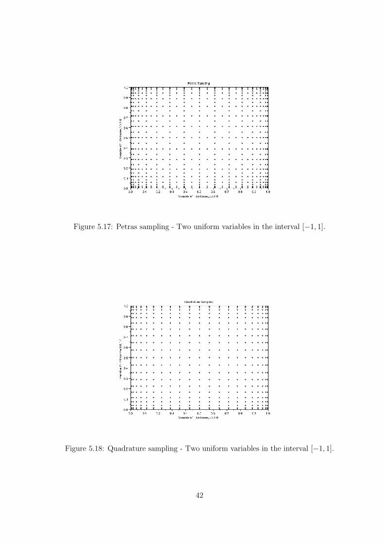
Figure 5.17: Petras sampling - Two uniform variables in the interval [−1, 1].

Figure 5.18: Quadrature sampling - Two uniform variables in the interval [−1, 1].

42

Figure 5.19: Sobol sampling - Two uniform variables in the interval [−1, 1].

43

Chapter 6

The polychaos class

6.1 Introduction

The polychaos class allows to manage a polynomial chaos expansion. The coefficients of theexpansion are computed based on given numerical experiments which creates the associationbetween the inputs and the outputs. Once computed, the expansion can be used as a regularfunction. The mean, standard deviation or quantile can also be directly retrieved.

The tool allows to get the following results:

• mean,

• variance,

• quantile,

• correlation, etc...

Moreover, we can generate the C source code which computes the output of the polynomial chaosexpansion. This C source code is stand-alone, that is, it is independent of both the NISP libraryand Scilab. It can be used as a meta-model.

The figure 6.1 presents the most commonly used methods available in the polychaos class.More methods are presented in figure 6.2. The inline help contains the detailed calling sequencefor each function and will not be repeated here. More than 50 methods are available and most ofthem will not be presented here.

More informations about the Oriented Object system used in this toolbox can be found in thesection 4.2.2.

6.2 Examples

In this section, we present to examples of use of the polychaos class.

6.2.1 Product of two random variables

In this section, we present the polynomial expansion of the product of two random variables.We analyse the Scilab script and present the methods which are available to perform the sensi-

44

Constructorspc = polychaos_new ( file )

pc = polychaos_new ( srv , ny )

pc = polychaos_new ( pc , nopt , varopt )

Methodspolychaos_setsizetarget ( pc , np )

polychaos_settarget ( pc , output )

polychaos_setinput ( pc , invalue )

polychaos_setdimoutput ( pc , ny )

polychaos_setdegree ( pc , no )

polychaos_getvariance ( pc )

polychaos_getmean ( pc )

Destructorpolychaos_destroy (pc)

Static methodstokenmatrix = polychaos_tokens ()

nb = polychaos_size ()

Figure 6.1: Outline of the methods of the polychaos class

tivity analysis. This script is based on the NISP methodology, which has been presented in theIntroduction chapter. We will use the figure 1.1 as a framework and will follow the steps in order.

In the following Scilab script, we define the function Example which takes a vector of size 2 asinput and returns a scalar as output.

function y = Exemple (x)y(:,1) = x(:,1) .* x(:,2)

endfunction

We now create a collection of two stochastic (normalized) random variables. Since the ran-dom variables are normalized, we use the default parameters of the randvar_new function. Thenormalized collection is stored in the variable srvx.

vx1 = randvar_new("Normale");vx2 = randvar_new("Uniforme");srvx = setrandvar_new ();setrandvar_addrandvar ( srvx , vx1 );setrandvar_addrandvar ( srvx , vx2 );

We create a collection of two uncertain parameters. We explicitely set the parameters of eachrandom variable, that is, the first Normal variable is associated with a mean equal to 1.0 anda standard deviation equal to 0.5, while the second Uniform variable is in the interval [1.0, 2.5].This collection is stored in the variable srvu.

vu1 = randvar_new("Normale" ,1.0 ,0.5);vu2 = randvar_new("Uniforme" ,1.0 ,2.5);srvu = setrandvar_new ();setrandvar_addrandvar ( srvu , vu1 );setrandvar_addrandvar ( srvu , vu2 );

45

Methodsoutput = polychaos_gettarget ( pc )

np = polychaos_getsizetarget ( pc )

polychaos_getsample ( pc , k , ovar )

polychaos_getquantile ( pc , k )

polychaos_getsample ( pc )

polychaos_getquantile ( pc , alpha )

polychaos_getoutput ( pc )

polychaos_getmultind ( pc )

polychaos_getlog ( pc )

polychaos_getinvquantile ( pc , threshold )

polychaos_getindextotal ( pc )

polychaos_getindexfirst ( pc )

ny = polychaos_getdimoutput ( pc )

nx = polychaos_getdiminput ( pc )

p = polychaos_getdimexp ( pc )

no = polychaos_getdegree ( pc )

polychaos_getcovariance ( pc )

polychaos_getcorrelation ( pc )

polychaos_getanova ( pc )

polychaos_generatecode ( pc , filename , funname )

polychaos_computeoutput ( pc )

polychaos_computeexp ( pc , srv , method )

polychaos_computeexp ( pc , pc2 , invalue , varopt )

polychaos_buildsample ( pc , type , np , order )

Figure 6.2: More methods from the polychaos class

46

The first design of experiment is build on the stochastic set srvx and based on a Quadraturetype of DOE. Then this DOE is transformed into a DOE for the uncertain collection of parameterssrvu.

degre = 2;setrandvar_buildsample ( srvx , "Quadrature" , degre );setrandvar_buildsample ( srvu , srvx );

The next steps will be to create the polynomial and actually perform the DOE. But beforedoing this, we can take a look at the DOE associated with the stochastic and uncertain collectionof random variables. We can use the setrandvar_getsample twice and get the following output.

-->setrandvar_getsample(srvx)ans =

- 1.7320508 0.1127017- 1.7320508 0.5- 1.7320508 0.8872983

0. 0.11270170. 0.50. 0.88729831.7320508 0.11270171.7320508 0.51.7320508 0.8872983

-->setrandvar_getsample(srvu)ans =

0.1339746 1.16905250.1339746 1.750.1339746 2.33094751. 1.16905251. 1.751. 2.33094751.8660254 1.16905251.8660254 1.751.8660254 2.3309475

These two matrices are a 9×2 matrices, where each line represents an experiment and each columnrepresents an input random variable. The stochastic (normalized) srvx DOE has been createdfirst, then the srvu has been deduced from srvx based on random variable transformations.

We now use the polychaos_new function and create a new polynomial pc. The number ofinput variables corresponds to the number of variables in the stochastic collection srvx, that is2, and the number of output variables is given as the input argument ny. In this particular case,the number of experiments to perform is equal to np=9, as returned by the setrandvar_getsize

function. This parameter is passed to the polynomial pc with the polychaos_setsizetarget

function.

ny = 1;pc = polychaos_new ( srvx , ny );np = setrandvar_getsize(srvx);polychaos_setsizetarget(pc,np);

47

In the next step, we perform the simulations prescribed by the DOE. We perform this loop inthe Scilab language and make a loop over the index k, which represents the index of the currentexperiment, while np is the total number of experiments to perform. For each loop, we get theinput from the uncertain collection srvu with the setrandvar_getsample function, pass it tothe Exemple function, get back the output which is then transferred to the polynomial pc by thepolychaos_settarget function.

inputdata = setrandvar_getsample(srvu);outputdata = Exemple(inputdata );polychaos_settarget(pc,outputdata );

We can compute the polynomial expansion based on numerical integration so that the coeffi-cients of the polynomial are determined. This is done with the polychaos_computeexp function,which stands for ”compute the expansion”.

polychaos_setdegree(pc,degre);polychaos_computeexp(pc,srvx ,"Integration");

Everything is now ready for the sensitivity analysis. Indeed, the polychaos_getmean returnsthe mean while the polychaos_getvariance returns the variance.

average = polychaos_getmean(pc);var = polychaos_getvariance(pc);mprintf("Mean = %f\n",average );mprintf("Variance = %f\n",var);mprintf("Indice de sensibilite du 1er ordre\n");mprintf(" Variable X1 = %f\n",polychaos_getindexfirst(pc ,1));mprintf(" Variable X2 = %f\n",polychaos_getindexfirst(pc ,2));mprintf("Indice de sensibilite Totale\n");mprintf(" Variable X1 = %f\n",polychaos_getindextotal(pc ,1));mprintf(" Variable X2 = %f\n",polychaos_getindextotal(pc ,2));


Mean = 1.750000Variance = 1.000000Indice de sensibilite du 1er ordre

Variable X1 = 0.765625Variable X2 = 0.187500

Indice de sensibilite TotaleVariable X1 = 0.812500Variable X2 = 0.234375

In order to free the memory required for the computation, it is necessary to delete all theobjects created so far.

polychaos_destroy(pc);randvar_destroy(vu1);randvar_destroy(vu2);randvar_destroy(vx1);randvar_destroy(vx2);setrandvar_destroy(srvu);setrandvar_destroy(srvx);

48

Prior to destroying the objects, we can inquire a little more about the density of the outputof the chaos polynomial. In the following script, we create a Latin Hypercube Sampling made of10 000 points. Then get the output of the polynomial on these inputs and plot the histogram ofthe output.

polychaos_buildsample(pc,"Lhs" ,10000 ,0);sample_output = polychaos_getsample(pc);scf();histplot (50, sample_output );xtitle("Product function - Empirical Histogram","X","P(X)");


0.00

0.05

0.10

0.15

0.20

0.25

0.30

0.35

0.40

0.45

-3 -2 -1 0 1 2 3 4 5 6 7

Product function - Empirical Histogram

X

P(X

)

Figure 6.3: Product function - Histogram of the output on a LHS design with 10000 experiments.

We may explore the following topics.

• Perform the same analysis where the variable X2 is a normal variable with mean 2 andstandard deviation 2.

• Check that the development in polynomial chaos on a Hermite-Hermite basis does not allowto get exact results. See that the convergence can be obtained by increasing the degree.

• Check that the development on a basis Hermite-Legendre allows to get exact results withdegree 2.

6.2.2 A note on performance

In this section, we emphasize vectorization which can be used to improve the performance of ascript when we compute the output of a function on a given sampling.

49

In order to use vectorization, the core feature that we used in the Exemple is the use of theelementwise multiplication, denoted by .*. In the Exemple function below (reproduced here forsimplicity), the input x is a np-by-2 matrix of doubles, where np is the number of experiments,and y is a np-by-1 matrix of doubles.

function y = Exemple (x)y(:,1) = x(:,1) .* x(:,2)

endfunction

The elementwise multiplication allows to multiply the two first columns of x, and sets the resultinto the output y, in one single statement. Since Scilab uses optimized numerical libraries, thisallows to get the best performance in most situations.

In the previous section, we have shown that we can compute the output of the Exemple

function in one single call to the function.

outputdata = Exemple(inputdata );

This call allows to produce all the outputs as fast as possible and is the recommended method.The reason is that the previous script lets Scilab perform computations with large matrices.

In fact, there is another, slower, method to perform the same computation. We make a loopover the index k, which represents the index of the current experiment, while np is the totalnumber of experiments to perform. For each loop, we get the input from the uncertain collectionsrvu with the setrandvar_getsample function, pass it to the Exemple function, get back theoutput which is then transferred to the polynomial pc by the polychaos_settarget function.

// This is slow.for k=1:np

inputdata = setrandvar_getsample(srvu ,k);outputdata = Exemple(inputdata );mprintf ( "Experiment #%d , input =[%f %f], output = %f\n", k, ..

inputdata (1), inputdata (2) , outputdata )polychaos_settarget(pc,k,outputdata );

end


Experiment #1, input =[0.133975 1.169052] , output = 0.156623Experiment #2, input =[0.133975 1.750000] , output = 0.234456Experiment #3, input =[0.133975 2.330948] , output = 0.312288Experiment #4, input =[1.000000 1.169052] , output = 1.169052Experiment #5, input =[1.000000 1.750000] , output = 1.750000Experiment #6, input =[1.000000 2.330948] , output = 2.330948Experiment #7, input =[1.866025 1.169052] , output = 2.181482Experiment #8, input =[1.866025 1.750000] , output = 3.265544Experiment #9, input =[1.866025 2.330948] , output = 4.349607

While the previous script is perfectly correct, it can be very slow when the number of ex-periments is large. This is because the interpreter has to perform a large number of loops withmatrices of small size. In general, this produces much slower script and should be avoided. Moredetails on this topic are presented in [2].

50

6.2.3 The Ishigami test case

In this section, we present the Ishigami test case.The function Exemple is the model that we consider in this numerical experiment. This

function takes a vector of size 3 in input and returns a scalar output.

function y = Exemple (x)a=7.b=0.1s1=sin(x(:,1))s2=sin(x(:,2))y(:,1) = s1 + a.*s2.*s2 + b.*x(: ,3).*x(: ,3).*x(: ,3).*x(: ,3).*s1

endfunction

We create 3 uncertain parameters which are uniform in the interval [−π, π] and put theserandom variables into the collection srvu.

rvu1 = randvar_new("Uniforme",-%pi ,%pi);rvu2 = randvar_new("Uniforme",-%pi ,%pi);rvu3 = randvar_new("Uniforme",-%pi ,%pi);

srvu = setrandvar_new ();setrandvar_addrandvar ( srvu , rvu1);setrandvar_addrandvar ( srvu , rvu2);setrandvar_addrandvar ( srvu , rvu3);

The collection of stochastic variables is created with the function setrandvar_new. The callingsequence srvx = setrandvar_new( nx ) allows to create a collection of nx=3 random variablesuniform in the interval [0, 1]. Then we create a Petras DOE for the stochastic collection srvx andtransform it into a DOE for the uncertain parameters srvu.

nx = setrandvar_getdimension ( srvu );srvx = setrandvar_new( nx );degre = 9;setrandvar_buildsample(srvx ,"Petras",degre );setrandvar_buildsample( srvu , srvx );

We use the polychaos_new function and create the new polynomial pc with 3 inputs and 1output.

noutput = 1;pc = polychaos_new ( srvx , noutput );

The next step allows to perform the simulations associated with the DOE prescribed by thecollection srvu. Here, we must perform np=751 experiments.

np = setrandvar_getsize(srvu);polychaos_setsizetarget(pc,np);inputdata = setrandvar_getsample(srvu);outputdata = Exemple(inputdata );polychaos_settarget(pc ,outputdata );

We can now compute the polynomial expansion by integration.

polychaos_setdegree(pc ,degre );polychaos_computeexp(pc,srvx ,"Integration");

51

Everything is now ready so that we can do the sensitivy analysis, as in the following script.

average = polychaos_getmean(pc);var = polychaos_getvariance(pc);mprintf("Mean = %f\n",average );mprintf("Variance = %f\n",var);mprintf("First order sensitivity index\n");mprintf(" Variable X1 = %f\n",polychaos_getindexfirst(pc ,1));mprintf(" Variable X2 = %f\n",polychaos_getindexfirst(pc ,2));mprintf(" Variable X3 = %f\n",polychaos_getindexfirst(pc ,3));mprintf("Total sensitivity index\n");mprintf(" Variable X1 = %f\n",polychaos_getindextotal(pc ,1));mprintf(" Variable X2 = %f\n",polychaos_getindextotal(pc ,2));mprintf(" Variable X3 = %f\n",polychaos_getindextotal(pc ,3));


Mean = 3.500000Variance = 13.842473First order sensitivity index

Variable X1 = 0.313953Variable X2 = 0.442325Variable X3 = 0.000000

Total sensitivity indexVariable X1 = 0.557675Variable X2 = 0.442326Variable X3 = 0.243721

We now focus on the variance generated by the variables #1 and #3. We set the groupto the empty group with the polychaos_setgroupempty function and add variables with thepolychaos_setgroupaddvar function.

groupe = [1 3];polychaos_setgroupempty ( pc );polychaos_setgroupaddvar ( pc , groupe (1) );polychaos_setgroupaddvar ( pc , groupe (2) );mprintf("Fraction of the variance of a group of variables\n");mprintf(" Groupe X1 et X2 =%f\n",polychaos_getgroupind(pc));


Fraction of the variance of a group of variablesGroupe X1 et X2 =0.557674

The function polychaos_getanova prints the functionnal decomposition of the normalizedvariance.

polychaos_getanova(pc);


1 0 0 : 0.3139530 1 0 : 0.4423251 1 0 : 1.55229e-0090 0 1 : 8.08643e-031

52

1 0 1 : 0.2437210 1 1 : 7.26213e-0311 1 1 : 1.6007e-007

We can compute the density function associated with the output variable of the function. Inorder to compute it, we use the polychaos_buildsample function and create a Latin HypercubeSampling with 10000 experiments. The polychaos_getsample function allows to quiery thepolynomial and get the outputs. We plot it with the histplot Scilab graphic function, whichproduces the figure 6.4.

polychaos_buildsample(pc,"Lhs" ,10000 ,0);sample_output = polychaos_getsample(pc);scf();histplot (50, sample_output)xtitle("Ishigami - Histogram");

151050-5-10

0.12

0.10

0.08

0.06

0.04

0.02

0.0020

Fonction Ishigami - Histogramme normalisé

Figure 6.4: Ishigami function - Histogram of the output of the chaos polynomial on a LHS designwith 10 000 experiments.

We can plot a bar graph of the sensitivity indices, as presented in figure 6.5.

for i=1:nxindexfirst(i)= polychaos_getindexfirst(pc,i);indextotal(i)= polychaos_getindextotal(pc,i);

endscf();

53

bar(indextotal ,0.2,’blue ’);bar(indexfirst ,0.15,’yellow ’);legend (["Total" "First order"],pos =1);xtitle("Ishigami - Sensitivity indices");

Figure 6.5: Ishigami function - Sensitivity indices.

54

Chapter 7

An introduction to sensitivity analysis

In this chapter, we (extremely) briefly present the theory which is used in the library. This sectionis a tutorial introduction to the NISP module.

7.1 Sensitivity analysis

In this section, we present the sensitivity analysis and emphasize the difference between globaland local analysis.

Consider the model

Y = f(X), (7.1)

where X ∈ DX ⊂ Rp is the input and Y ∈ DY ⊂ Rm is the output of the model. The mapping fis presented in figure 7.1.

f

X Y

DX DY

Figure 7.1: Global analysis.

The assume that the input X is a random variable, so that the output variable Y is also arandom variable. We are interested in measuring the sensitivity of the output depending on theuncertainty of the input. More precisely, we are interested in knowing

• the input variables Xi which generate the most variability in the output Y,

• the input variables Xi which are not significant,

• a sub-space of the input variables where the variability is maximum,

• if input variables interacts.

55

Consider the mapping presented in figure 7.1. The f mapping transforms the domain DX intothe domain DY . If f is sufficiently smooth, small perturbations of X generate small perturbationsof Y . The local sensitivity analysis focuses on the behaviour of the mapping in the neighbourhoodof a particular point X ∈ DX toward a particular point Y ∈ DY . The global sensisitivity analysismodels the propagation of uncertainties transforming the whole set DX into the set DY .

In the following, we assume that there is only one output variable so that Y ∈ R.There are two types of analysis that we are going to perform, that is uncertainty analysis and

sensitivity analysis.In uncertainty analysis, we assume that fX is the probability density function of the variable

X and we are searching for the probability density function fY of the variable Y and by itscumulated density function FY (y) = P (Y ≤ y). This problem is difficult in the general case, andthis is why we often are looking for an estimate of the expectation of Y , as defined by

E(Y ) =

∫DX

yfY (y)dy, (7.2)

and an estimate of its variance

V (Y ) =

∫DX

(y − E(Y ))2fY (y)dy. (7.3)

We might also be interested in the computation of the probability over a threshold.In sensitivity analysis, we focus on the relative importance of the input variable Xi on the

uncertainty of Y. This way, we can order the input variables so that we can reduce the variabilityof the most important input variables, in order to, finally, reduce the variability of Y.

More details on this topic can be found in the papers of Homma and Saltelli [4] or in the workof Sobol [10]. The Thesis by Jacques [6] presents an overview of sensitivity analysis.

7.2 Standardized regression coefficients of affine models

In this section, we present the standardized regression coefficients of an affine model.Assume that the random variables Xi are independent, with mean E(Xi) and finite variances

V (Xi), for i = 1, 2, . . . , p. Let us consider the random variable Y as an affine function of thevariables Xi:

Y = β0 +∑

i=1,2,...,p

βiXi, (7.4)

where βi are real parameters, for i = 1, 2, . . . , p.The expectation of the random variable Y is

E(Y ) = β0 +∑

i=1,2,...,p

βiE(Xi). (7.5)

Since the variables Xi are independent, the variance of the sum of variables is the sum of thevariances. Hence,

V (Y ) = V (β0) +∑

i=1,2,...,p

V (βiXi), (7.6)

56

which leads to the equality

V (Y ) =∑

i=1,2,...,p

β2i V (Xi). (7.7)

Hence, each term β2i V (Xi) is the part of the total variance V (Y ) which is caused by the variable

Xi.

Definition 7.2.1. ( Standardized Regression Coefficient) The standardized regression coefficientis

SRCi =β2i V (Xi)

V (Y ), (7.8)

for i = 1, 2, . . . , p.

Hence, the sum of the standardized regression coefficients is one:

SRC1 + SRC2 + . . .+ SRCp = 1. (7.9)

7.3 Link with the linear correlation coefficients

In this section, we present the link between the linear correlation coefficients of an affine model,and the standardized regression coefficients.

Assume that the random variables Xi are independent, with mean E(Xi) and finite variancesV (Xi), for i = 1, 2, . . . , p. Let us consider the random variable Y , which depends linearily on thevariables Xi by the relationship 7.4.

The linear correlation coefficient between Y and Xi is

ρY,Xi=

Cov(Y,Xi)√V (Y )

√V (Xi)

, (7.10)

for i = 1, 2, . . . , p. In the particular case of the affine model 7.4, we have

Cov(Y,Xi) = Cov(β0, Xi) + β1Cov(X1, Xi) + β2Cov(X2, Xi) + . . .+ (7.11)

βiCov(Xi, Xi) + . . .+ βpCov(Xp, Xi). (7.12)

(7.13)

Since the random variables Xi are independent, we have Cov(Xj, Xi) = 0, for any j 6= i. There-fore,

Cov(Y,Xi) = βiCov(Xi, Xi) (7.14)

= βiV (Xi). (7.15)

Hence, the correlation coefficient can be simplified into

ρY,Xi=

βiV (Xi)√V (Y )

√V (Xi)

(7.16)

=βi√V (Xi)√V (Y )

. (7.17)

57

We square the previous equality and get

ρ2Y,Xi

=β2i V (Xi)

V (Y ). (7.18)

Therefore, the square of the linear correlation coefficient is equal to the first order sensitivityindex, i.e.

ρ2Y,Xi

= SRCi. (7.19)

7.4 An example of affine model

In this section, we present an example of an affine model, where the difference between local andglobal sensitivity is made clearer by the use of scatter plots.

Consider the four independent random variables Xi, for i = 1, 2, 3, 4. We assume that thevariables Xi are normally distributed, with zero mean and i2 variance.

Let us consider the affine model

Y = X1 +X2 +X3 +X4. (7.20)

Notice that the derivative of Y with respect to any of its input is equal to one, i.e.

∂Y

∂Xi

= 1, (7.21)

for i = 1, 2, 3, 4. This means that, locally, the inputs all have the same effect on the output. Aswe are going to see, all the input random variables do not have the same effect on the variabilityof the output Y .

We can immediately compute the expectation of the output Y . Since the input randomvariables are independent, we have

E(Y ) = E(X1) + E(X2) + E(X3) + E(X4). (7.22)

In our case, the input variables Xi have zero mean, so that the output random variable Y alsohas a zero mean.

Let us compute the standardized regression coefficients of this model. By hypothesis, thevariance of each variable is

V (X1) = 1, V (X2) = 4, (7.23)

V (X3) = 9, V (X4) = 16. (7.24)

Since the variables are independent, the variance of the output Y is

V (Y ) = V (X1) + V (X2) + V (X3) + V (X4) = 30. (7.25)

The standardized regression coefficient is

SRCi =β2i V (Xi)

V (Y )=i2

30, (7.26)

58

for i = 1, 2, 3, 4. More specifically, we have

SRC1 =1

30, SRC2 =

4

30, (7.27)

SRC3 =9

30, SRC4 =

16

30. (7.28)

We have the following inequalities:

SRC4 > SRC3 > SRC2 > SRC1. (7.29)

This means that the variable which causes the most variance in the output is X4, while thevariable which causes the least variance in the output is X1.

The script below performs the analysis with the NISP module. The sampling is based on aLatin Hypercube Sampling design with 5000 points.

function y = Exemple (x)y(:) = x(:,1) + x(:,2) + x(:,3) + x(:,4)

endfunction

function r = lincorrcoef ( x , y )// Returns the linear correlation coefficient of x and y.// The variables are expected to be column matrices with the same size.x = x(:)y = y(:)mx = mean(x)my = mean(y)sx = sqrt(sum((x-mx ).^2))sy = sqrt(sum((y-my ).^2))r = (x-mx)’*(y-my) / sx / sy

endfunction

// Initialisation de la graine aleatoirenisp_initseed ( 0 );

// Create the random variables.rvu1 = randvar_new("Normale" ,0,1);rvu2 = randvar_new("Normale" ,0,2);rvu3 = randvar_new("Normale" ,0,3);rvu4 = randvar_new("Normale" ,0,4);srvu = setrandvar_new ();setrandvar_addrandvar ( srvu , rvu1);setrandvar_addrandvar ( srvu , rvu2);setrandvar_addrandvar ( srvu , rvu3);setrandvar_addrandvar ( srvu , rvu4);// Create a sampling by a Latin Hypercube Sampling with size 5000.nbshots = 5000;setrandvar_buildsample(srvu , "Lhs",nbshots );sampling = setrandvar_getsample(srvu);// Perform the experiments.y=Exemple(sampling );

59

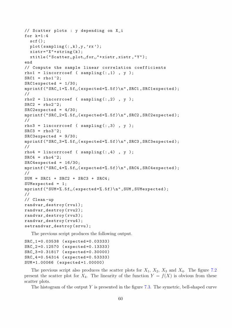
// Scatter plots : y depending on X_ifor k=1:4

scf();plot(sampling(:,k),y,’rx ’);xistr="X"+string(k);xtitle("Scatter plot for "+xistr ,xistr ,"Y");

end// Compute the sample linear correlation coefficientsrho1 = lincorrcoef ( sampling (:,1) , y );SRC1 = rho1 ^2;SRC1expected = 1/30;mprintf("SRC_1=%.5f (expected=%.5f)\n",SRC1 ,SRC1expected );//rho2 = lincorrcoef ( sampling (:,2) , y );SRC2 = rho2 ^2;SRC2expected = 4/30;mprintf("SRC_2=%.5f (expected=%.5f)\n",SRC2 ,SRC2expected );//rho3 = lincorrcoef ( sampling (:,3) , y );SRC3 = rho3 ^2;SRC3expected = 9/30;mprintf("SRC_3=%.5f (expected=%.5f)\n",SRC3 ,SRC3expected );//rho4 = lincorrcoef ( sampling (:,4) , y );SRC4 = rho4 ^2;SRC4expected = 16/30;mprintf("SRC_4=%.5f (expected=%.5f)\n",SRC4 ,SRC4expected );//SUM = SRC1 + SRC2 + SRC3 + SRC4;SUMexpected = 1;mprintf("SUM=%.5f (expected=%.5f)\n",SUM ,SUMexpected );//// Clean -uprandvar_destroy(rvu1);randvar_destroy(rvu2);randvar_destroy(rvu3);randvar_destroy(rvu4);setrandvar_destroy(srvu);


SRC_1 =0.03538 (expected =0.03333)SRC_2 =0.12570 (expected =0.13333)SRC_3 =0.31817 (expected =0.30000)SRC_4 =0.54314 (expected =0.53333)SUM =1.00066 (expected =1.00000)

The previous script also produces the scatter plots for X1, X2, X3 and X4. The figure 7.2present the scatter plot for X4. The linearity of the function Y = f(X) is obvious from thesescatter plots.

The histogram of the output Y is presented in the figure 7.3. The symetric, bell-shaped curve

60

Figure 7.2: Scatter plot for an affine model - Variable X4.

makes it clear that the output Y is a normal random variable. Indeed, we know from the previousanalysis that the mean of Y is zero, and its variance is 30.

7.5 Sensitivity analysis for nonlinear models

Let us focus on one particular input Xi of the model f , with i = 1, 2, . . . , p. If we set Xi to aparticular value, say xi for example, then the variance of the output Y may decrease or increase,depending on the value of xi, because the variable Xi is not random anymore. We can thenmeasure the conditionnal variance given Xi = xi, denoted by V (Y |Xi = xi).

Since Xi is a random variable, then the conditionnal variance V (Y |Xi = xi) is a randomvariable. We have already emphasized that the variance V (Y ) can be smaller or larger thanV (Y |Xi = xi). The other problem is that, in most cases, we do not know where the value of Xi

is best fixed. It may sound reasonable to investigate V (Y |Xi = xi) when the random variable Xi

has its mean value, i.e. it may be interesting to computed V (Y |Xi = xi). But other values of Xi

might change the variance significantly, so that the result may not be interesting.It therefore sounds reasonable to average the measure V (Y |Xi = xi) over all possible values of

Xi. We are then interested in E(V (Y |Xi)). If Xi has a large weight in the variance V (Y ), thenE(V (Y |Xi)) is small.

The theorem of the total variance states that, if V (Y ) is finite, then

V (Y ) = V (E(Y |Xi)) + E(V (Y |Xi)). (7.30)

If Xi has a large weight in the variance V (Y ), then V (E(Y |Xi)) is large.

61

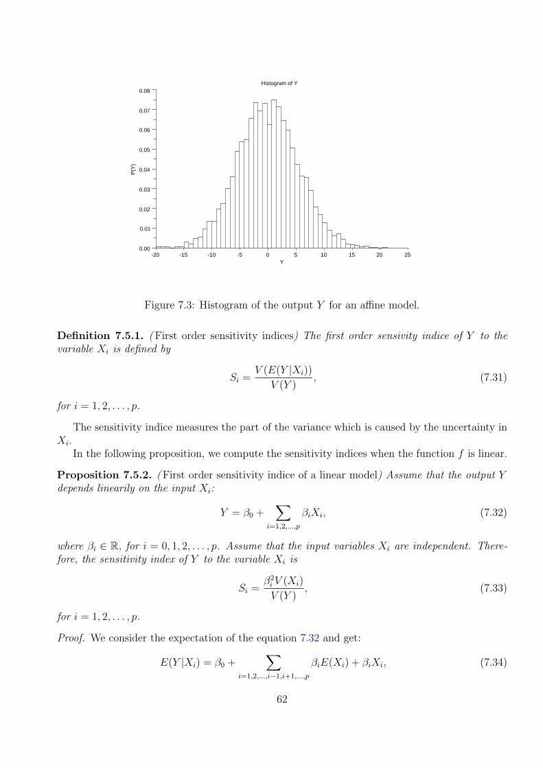
0.00

0.01

0.02

0.03

0.04

0.05

0.06

0.07

0.08

-20 -15 -10 -5 0 5 10 15 20 25

Histogram of Y

Y

P(Y

)

Figure 7.3: Histogram of the output Y for an affine model.

Definition 7.5.1. ( First order sensitivity indices) The first order sensivity indice of Y to thevariable Xi is defined by

Si =V (E(Y |Xi))

V (Y ), (7.31)

for i = 1, 2, . . . , p.

The sensitivity indice measures the part of the variance which is caused by the uncertainty inXi.

In the following proposition, we compute the sensitivity indices when the function f is linear.

Proposition 7.5.2. ( First order sensitivity indice of a linear model) Assume that the output Ydepends linearily on the input Xi:

Y = β0 +∑

i=1,2,...,p

βiXi, (7.32)

where βi ∈ R, for i = 0, 1, 2, . . . , p. Assume that the input variables Xi are independent. There-fore, the sensitivity index of Y to the variable Xi is

Si =β2i V (Xi)

V (Y ), (7.33)

for i = 1, 2, . . . , p.

Proof. We consider the expectation of the equation 7.32 and get:

E(Y |Xi) = β0 +∑

i=1,2,...,i−1,i+1,...,p

βiE(Xi) + βiXi, (7.34)

62

since the expection of a sum is the sum of expectations. Then,

V (E(Y |Xi)) = V (βiXi) (7.35)

= β2i V (Xi), (7.36)

since the variance of a constant term is zero. This immediately leads to the equation 7.33.

Hence, if we make the assumption that a model is affine, then the empirical linear correlationcoefficient can be used to estimate the sensitivity indices.

We now discuss various particular values of the first order sensitivity indices of a generalfunction f .

The following proposition allows to support the idea that, if Si = 0, then Y is uncorrelated toXi on average.

Proposition 7.5.3. Assume that the output Y depends on the input Xi:

Y = f(X1, X2, . . . , Xp) (7.37)

where the input variables Xi are independent. If, for some i = 1, 2, . . . , p, the variables Y and Xi

are independent, then Si = 0.

Proof. This is an immediate consequence of the definition of Si. Assume that i is an integer in theset {1, 2, . . . , p} and assume that Y and Xi are independent. Then the random variable E(Y |Xi)does not depend on Xi. Therefore, the conditionnal expectation E(Y |Xi) is a constant. Hence,its variance is zero.

We emphasize that the previous result is true only on average. We also emphasize that theconverse is not true, i.e. the equality Si = 0 does not imply that Y and Xi are independent. Thisis because it might happen that the variable Xi interact with some other variable Xj, with j 6= i.In this case, the variable Xi will be influential to the output Y by the mean of the interaction.In the section 7.6, we give an example of such a particular case.

TODO : the case Si = 1

7.6 The product of two variables

In this example, we consider a non-linear, non-additive model made of the product of two inde-pendent random variables. The goal of this example is to show that, in some cases, we have toconsider the interations between the variables.

Consider the function

Y = X1X2, (7.38)

whereX1 andX2 are two independent normal random variables with mean µ1 and µ2 and variancesσ2

1 and σ22.

Let us compute the expectation of the random variable Y . The expectation of Y is

E(Y ) =

∫ ∞−∞

∫ ∞−∞

X1X2F (X1, X2)dx1dx2, (7.39)

63

where F (x1, x2) is the joint probability distribution function of the variables X1 and X2. SinceX1 and X2 are independent variables, we have

F (x1, x2) = F1(X1)F2(X2), (7.40)

where F1 is the probability distribution function of X1 and F2 is the probability distributionfunction of X2. Then, we have

E(Y ) =

∫ ∞−∞

∫ ∞−∞

X1X2F1(X1)F2(X2)dx1dx2 (7.41)

=

(∫ ∞−∞

X1F1(X1)dx1

)(∫ ∞−∞

X2F2(X2)dx2

). (7.42)

= E(X1)E(X2). (7.43)

Therefore,

E(Y ) = µ1µ2. (7.44)

The variance of Y is

V (Y ) = E(Y 2)− E(Y )2. (7.45)

The expectation E(Y 2) is

E(Y 2) =

∫ ∞−∞

∫ ∞−∞

(X1X2)2F (x1, x2)dx1dx2 (7.46)

=

∫ ∞−∞

∫ ∞−∞

(X1X2)2F1(X1)F2(X2)dx1dx2 (7.47)

=

(∫ ∞−∞

X21F1(X1)dx1

)(∫ ∞−∞

X22F2(X2)dx2

), (7.48)

= E(X21 )E(X2

2 ). (7.49)

Now, we have

V (X1) = E(X21 )− E(X1)

2, V (X2) = E(X22 )− E(X2)

2, (7.50)

which leads to

E(X21 ) = V (X1) + E(X1)

2, E(X22 ) = V (X2) + E(X2)

2. (7.51)

Therefore,

E(Y 2) = (V (X1) + E(X1)2)(V (X2) + E(X2)

2) (7.52)

= (σ21 + µ2

1)(σ22 + µ2

2). (7.53)

Finally, we get

V (Y ) = (σ21 + µ2

1)(σ22 + µ2

2)− (µ1µ2)2. (7.54)

64

We can expand the previous equality and get

V (Y ) = σ21σ

22 + σ2

1µ22 + µ2

1σ22 + µ2

1µ22 − (µ1µ2)

2. (7.55)

The last two terms of the previous equality can be simplified, so that we get

V (Y ) = σ21σ

22 + σ2

1µ22 + µ2

1σ22. (7.56)

The sensitivity indices can be computed from the definitions

S1 =V (E(Y |X1))

V (Y ), S2 =

V (E(Y |X2))

V (Y ). (7.57)

We have E(Y |X1) = E(X2)X1 = µ2X1. Similarily, E(Y |X2) = µ1X2. Hence

S1 =V (µ2X1)

V (Y ), S2 =

V (X2)

V (Y ). (7.58)

We get

S1 =µ2

2V (X1)

V (Y ), S2 =

µ21V (X2)

V (Y ). (7.59)

Finally, the first order sensitivity indices are

S1 =µ2

2σ21

V (Y ), S2 =

µ21σ

22

V (Y ). (7.60)

Since σ21σ

22 ≥ 0, we have

µ22σ

21 + µ2

1σ22 ≤ V (Y ) = σ2

1σ22 + σ2

1µ22 + µ2

1σ22. (7.61)

We divide the previous inequality by V (Y ), and get

µ22σ

21

V (Y )+µ2

1σ22

V (Y )≤ 1. (7.62)

Therefore, the sum of the first order sensitivity indices satisfies the inequality

S1 + S2 ≤ 1. (7.63)

Hence, in this example, one part of the variance V (Y ) cannot be explained neither by X1

alone, or by X2 alone, because it is caused by the interactions between X1 and X2. We define byS1,2 the sensitivity index associated with the group of variables (X1, X2) as

S1,2 = 1− S1 − S2 =σ2

1σ22

V (Y ). (7.64)

The following Scilab script performs the sensitivity analysis on the previous example. Weconsider two normal variables, where the first variable has mean 1.5 and standard deviation 0.5while the second variable has mean 3.5 and standard deviation 2.5.

The following function defines the product of the X1 and X2 variables. Each column corre-spond to an input random variable and each row correspond to a numerical experiment.

65

function y = Exemple (x)y(:,1) = x(:,1) .* x(: ,2);

endfunction

The following function computes the exact sensitivity indices for the product function.

function exact = product_saexact ( mu1 , sigma1 , mu2 , sigma2 )// Exact results for the Product functionexact.expectation = mu1*mu2;exact.var = mu2^2* sigma1 ^2 + mu1^2* sigma2 ^2 + sigma1 ^2* sigma2 ^2;// Sensitivity indices.exact.S1 = ( mu2^2* sigma1 ^2 ) / exact.var;exact.S2 = ( mu1^2* sigma2 ^2 ) / exact.var;exact.S12 = ( sigma1 ^2 * sigma2 ^2 ) / exact.var;exact.ST1 = exact.S1 + exact.S12;exact.ST2 = exact.S2 + exact.S12;

endfunction

The following script computes the exact sensitivity indices in the particular case where wherethe first variable has mean 1.5 and standard deviation 0.5 while the second variable has mean 3.5and standard deviation 2.5.

// First variable// Normalmu1 = 1.5;sigma1 = 0.5;// Second variable// Normalmu2 = 3.5;sigma2 = 2.5;exact = product_saexact ( mu1 , sigma1 , mu2 , sigma2 )


-->exact = product_saexact ( mu1 , sigma1 , mu2 , sigma2 )exact =

expectation: 5.25var: 18.6875S1: 0.1638796S2: 0.7525084S12: 0.0836120ST1: 0.2474916ST2: 0.8361204

We can see that the sum of the two first order indices S1 and S2 is lower than 1.

-->exact.S1+exact.S2ans =

0.9163880

This is because the interaction between the two variables X1 and X2 and is measured by S1,2 =0.0836120.

The scatter plots for this function is presented in the figures 7.4 and fig-product-scatter2.These scatter plots are based on a Monte-Carlo simulation with 1000 experiments. It is clear thatthe variability of Y increases with the magnitude of X1 or X2.

66

Figure 7.4: Scatter plot for the product function X1 ·X2 - Variable X1.

Figure 7.5: Scatter plot for the product function X1 ·X2 - Variable X2.

67

The histogram of the output Y is presented in the figure 7.6.

0.00

0.02

0.04

0.06

0.08

0.10

0.12

-10 -5 0 5 10 15 20 25

Histogram of Y

Y

P(Y

)

Figure 7.6: Histogram of Y for the product function X1 ·X2.

In the following script, we perform the sensitivity analysis with the NISP library.

// 1. Two stochastic (normalized) variablesvx1 = randvar_new("Normale");vx2 = randvar_new("Normale");// 2. A collection of stoch. variables.srvx = setrandvar_new ();setrandvar_addrandvar ( srvx ,vx1);setrandvar_addrandvar ( srvx ,vx2);// 3. Two uncertain parametersvu1 = randvar_new("Normale",mu1 ,sigma1 );vu2 = randvar_new("Normale",mu2 ,sigma2 );// 4. A collection of uncertain parameterssrvu = setrandvar_new ();setrandvar_addrandvar ( srvu ,vu1);setrandvar_addrandvar ( srvu ,vu2);// 5. Create the Design Of Experimentsdegre = 2;setrandvar_buildsample(srvx ,"Quadrature",degre);setrandvar_buildsample( srvu , srvx );// 6. Create the polynomialny = 1;pc = polychaos_new ( srvx , ny );np = setrandvar_getsize(srvx);mprintf("Number of experiments : %d\n",np);

68

polychaos_setsizetarget(pc,np);// 7. Perform the DOEinputdata = setrandvar_getsample(srvu);outputdata = Exemple(inputdata );polychaos_settarget(pc,outputdata );// 8. Compute the coefficients of the polynomial expansionpolychaos_setdegree(pc,degre);polychaos_computeexp(pc,srvx ,"Integration");// 9. Get the sensitivity indicesaverage = polychaos_getmean(pc);var = polychaos_getvariance(pc);mprintf("Mean = %f (expectation = %f)\n",average ,exact.expectation );mprintf("Variance = %f (expectation = %f)\n",var ,exact.var);mprintf("First order sensitivity index\n");S1 = polychaos_getindexfirst(pc ,1);mprintf(" Variable X1 = %f (expectation = %f)\n",S1,exact.S1);re = abs(S1- S1_expectation )/ S1_expectation;mprintf(" Relative Error = %f\n", re);S2 = polychaos_getindexfirst(pc ,2);mprintf(" Variable X2 = %f (expectation = %f)\n",S2,exact.S2);re = abs(S2- S2_expectation )/ S2_expectation;mprintf(" Relative Error = %f\n", re);

mprintf("Total sensitivity index\n");ST1 = polychaos_getindextotal(pc ,1);mprintf(" Variable X1 = %f\n",ST1);ST2 = polychaos_getindextotal(pc ,2);mprintf(" Variable X2 = %f\n",ST2);// Clean -uppolychaos_destroy(pc);randvar_destroy(vu1);randvar_destroy(vu2);randvar_destroy(vx1);randvar_destroy(vx2);setrandvar_destroy(srvu);setrandvar_destroy(srvx);


Mean = 5.250000 (expectation = 5.250000)Variance = 18.687500 (expectation = 18.687500)First order sensitivity index

Variable X1 = 0.163880 (expectation = 0.163880)Relative Error = 0.000000

Variable X2 = 0.752508 (expectation = 0.752508)Relative Error = 0.000000

Total sensitivity indexVariable X1 = 0.247492Variable X2 = 0.836120

We see that the polynomial chaos performs an exact computation.

69

We are now considering the fact that Si = 0 does not imply that the output Y is independentof Xi. We consider the case of the product function to show an example of this.

We consider the case where µ2 = 0. If we plug the equality µ2 = 0 into the equations 7.60, weget S1 = 0. But the equation Y = X1X2 is clear about the fact that Y is not independent of X1

at all! The following script allows to compute the sensitivity indices in such a case.

mu1 = 0.1;sigma1 = 0.5;mu2 = 0;sigma2 = 2.5;exact = product_saexact ( mu1 , sigma1 , mu2 , sigma2 )


-->exact = product_saexact ( mu1 , sigma1 , mu2 , sigma2 )exact =

expectation: 0var: 1.625S1: 0S2: 0.0384615S12: 0.9615385ST1: 0.9615385ST2: 1

We see that S1 = 0 and S2 is small. There again, the effect on the output Y is caused by theinteraction between X1 and X2, which is measured by S1,2 = 0.9615385. In other words, 96% ofthe variance of the output Y is caused by the interaction of X1 and X2.

The figure 7.7 presents the scatter plot of the output variable Y . The fact that X2 hasa zero mean implies that, whatever the value of X1, the expectation value of Y is zero, i.e.E(Y |X1 = x1) = 0, for any x1. As a result, the variance V (E(Y |X1)) = 0. This can be seen inthe figure 7.7. The conditionnal expectation E(Y |X1) is the mean of Y given a value of X1 andso can be computed by averaging the values of Y on a vertical line X1 = x1. Since the valuesof Y are symetrically dispersed under and over the line Y = 0, the expectation E(Y |X1) is zero.Hence the variance of the averaged values of Y is also zero.

7.7 Sobol decomposition

Sobol [10] introduced the sensitivity index based on V (E(Y |Xi)) by decomposing the function fas a sum of function with an increasing number of parameters.

Proposition 7.7.1. ( Sobol decomposition) Consider the function f

Y = f(x1, x2, . . . , xp), (7.65)

where x1, . . . , xp ∈ [0, 1]. If f can be integrated in [0, 1]p, then there is a unique decomposition

Y = f0 +∑

i=1,2,...,p

fi(xi) +∑

1≤i<j≤p

fi,j(xi, xj) + . . .+ f1,2,...,p(x1, x2, . . . , xp), (7.66)

where f0 is a constant and the function of the decomposition satisfy the equalities∫ 1

0

fi1,...,is(xi1 , . . . , xis)dxik = 0, (7.67)

70

Figure 7.7: Scatter plot for the product function X1 ·X2 when S1 = 0 - Variable X1.

for any k = 1, 2, . . . , s and any indices {i1, . . . , is} ⊂ {1, . . . , p}.

Example (Sobol decomposition) Consider the case p = 3, i.e. consider the function

Y = f(x1, x2, x3), (7.68)

where x1, x2, x3 ∈ [0, 1]. The Sobol decomposition theorem states that there exists functionsf1, f2, f3, f12, f13, f23 and f123 such that

f(x1, x2, x3) = f1(x1) + f2(x2) + f3(x3) + f12(x1, x2) + (7.69)

f13(x1, x3) + f23(x2, x3) + f123(x1, x2, x3), (7.70)

such that the integrals of f1, f2 and f3 satisfy∫ 1

0

f1(x1)dx1 = 0,

∫ 1

0

f2(x2)dx2 = 0,

∫ 1

0

f3(x3)dx3 = 0, (7.71)

such that the integrals of f12, f13 and f23 satisfy∫ 1

0

f12(x1, x2)dx1 = 0,

∫ 1

0

f12(x1, x2)dx2 = 0, (7.72)∫ 1

0

f13(x1, x3)dx1 = 0,

∫ 1

0

f13(x1, x3)dx3 = 0, (7.73)∫ 1

0

f23(x2, x3)dx2 = 0,

∫ 1

0

f23(x2, x3)dx3 = 0, (7.74)

71

and such that the integrals of f123 satisfy∫ 1

0

f123(x1, x2, x3)dx1 = 0,

∫ 1

0

f123(x1, x2, x3)dx2 = 0, (7.75)∫ 1

0

f123(x1, x2, x3)dx3 = 0. (7.76)

The equalities 7.67 mean that the integral of each function with respect to one of its variablesis zero. The immediate consequence of this is that the decomposition functions are orthogonal,i.e. ∫ 1

0

fi1,...,is(xi1 , . . . , xis)fj1,...,js(xj1 , . . . , xjs)dx1 . . . dxp = 0, (7.77)

if (i1, . . . , is) 6= (j1, . . . , js).This because if the two set of indices (i1, . . . , is) and (j1, . . . , js), this means that there is at

least one index k which appears in one index and not in the other. By the equality 7.67, thisimplies that if we integrate with respect to xk, then the integral is zero. Since the integral in 7.77is for all the variables, since implies that all the integral is zero.

We are now going to explicitely compute the decomposition functions f0, fi, fi,j, etc... byintegration the decomposition, using the orthogonality to simplify the results. If we integrate theequation 7.66 with respect to all the variables, we get∫ 1

0

f(x)dx = f0. (7.78)

Let us denote by x∼i the vector x without its i-th component, i.e.

x∼i = (x1, x2, . . . , xi−1, xi+1, . . . , xp). (7.79)

If we integrate the equation 7.66 with respect to all the variables except i, we get∫ 1

0

f(x)dx∼i = f0 + fi(xi). (7.80)

If we integrate the equation 7.66 with respect to all the variables except i and j, we get∫ 1

0

f(x)dx∼i,j = f0 + fi(xi) + fj(xj) + fi,j(xi, xj). (7.81)

If we integrate the equation 7.66 with respect to all the variables except i and j and k, we get∫ 1

0

f(x)dx∼i,j,k = f0 + fi(xi) + fj(xj) + fk(xk) + (7.82)

fi,j(xi, xj) + fi,k(xi, xk) + fj,k(xj, xk) + fi,j,k(xi, xj, xk). (7.83)

72

The previous computations allows to get the decomposition functions.

f0 =

∫ 1

0

f(x)dx (7.84)

fi(xi) = −f0 +

∫ 1

0

f(x)dx∼i (7.85)

fi,j(xi, xj) = −f0 − fi(xi)− fj(xj) +

∫ 1

0

f(x)dx∼i,j, (7.86)

fi,j,k(xi, xj, xk) = −f0 − fi(xi)− fj(xj)− fk(xk)− fi,j(xi, xj)− fi,k(xi, xk) (7.87)

−fj,k(xj, xk) +

∫ 1

0

f(x)dx∼i,j,k, (7.88)

until the last term

f1,2,...,p(x1, x2, . . . , xp) = f(x)− f0 −∑

i=1,2,...,p

fi(xi)− . . . (7.89)

−∑

1≤i1<...<ip−1≤p

fi1,...,ip−1(xi1 , . . . , xip−1). (7.90)

The last term is obviously so that the equality 7.66 is satisfied.We have considered a function where the variables are in [0, 1]p. In fact, when we consider

the more general model Y = f(X1, . . . , Xp) where the random variables Xi are independent anduniform in [0, 1]p, the decomposition 7.66 is still valid.

7.8 Decomposition of the expectation

We can consider the decomposition 7.66 in terms of expectation and variance.If we compute the expectation of Y by the expression 7.66 we get

E(Y ) = f0, (7.91)

which is an obvious consequence of the zero integral property 7.67.We can compute the first order decomposition functions fi, by computing the conditional

expectation with respect to Xi. Indeed, since the conditional expectation with respect to Xi is

E(Y |Xi) =

∫ 1

0

f(x)dx∼i, (7.92)

for all i = 1, 2, . . . , p, the equation 7.85 can be written as

fi(xi) = −f0 + E(Y |Xi). (7.93)

We now plug the equation 7.91 into the previous equality, and get

fi(xi) = E(Y |Xi)− E(Y ). (7.94)

73

Similarily, we can compute the first order decomposition functions fi,j, by computing theconditional expectation with respect to Xi and Xj. Indeed, since the conditional expectationwith respect to Xi is

E(Y |Xi, Xj) =

∫ 1

0

f(x)dx∼i,j, (7.95)

for all i = 1, 2, . . . , p, the equation 7.86 can be written as

fi,j(xi, xj) = −f0 − fi(xi)− fj(xj) + E(Y |Xi, Xj), (7.96)

= E(Y |Xi, Xj)− E(Y )− E(Y |Xi)− E(Y |Xj). (7.97)

Similarily, the equation 7.88 leads to

fi,j,k(xi, xj, xk) = −f0 − fi(xi)− fj(xj)− fk(xk)− fi,j(xi, xj)− fi,k(xi, xk) (7.98)

−fj,k(xj, xk) + E(Y |Xi, Xj, Xk). (7.99)

= E(Y |Xi, Xj, Xk)− E(Y )− E(Y |Xi)− E(Y |Xj)− E(Y |Xk) (7.100)

−E(Y |Xi, Xj)− E(Y |Xi, Xk)− E(Y |Xj, Xk). (7.101)

7.9 Decomposition of the variance

The variance of the function 7.65 can be decomposed into

V (Y ) =

p∑i=1

Vi +∑

1≤i<j≤p

Vij + . . .+ V1,2,...,p, (7.102)

where

Vi = V (E(Y |Xi)), (7.103)

Vij = V (E(Y |Xi, Xj))− Vi − Vj (7.104)

Vi,j,k = V (E(Y |Xi, Xj, Xk))− Vij − Vik − Vjk − Vi − Vj − Vk, (7.105)

. . . (7.106)

V1,2,...,p = V (Y )−p∑i=1

Vi −∑

1≤i,j≤p

Vij −∑

1≤i1<i2<...<ip−1≤p

Vi1i2...ip . (7.107)

The previous equality is straigtforward, since the equality 7.107 is so that the equality 7.102must be satisfied, i.e. the term V1,2,...,p is the difference between V (Y ) and all the variancesassociated with lower orders.

It can be proved that the terms of the variance decomposition 7.102 are the variances of thefunctions defined by 7.91, 7.94, 7.97, 7.101, i.e.

Vi1,i2,...,is = V (fi1,i2,...,is(Xi1 , Xi2 , . . . , Xis)), (7.108)

74

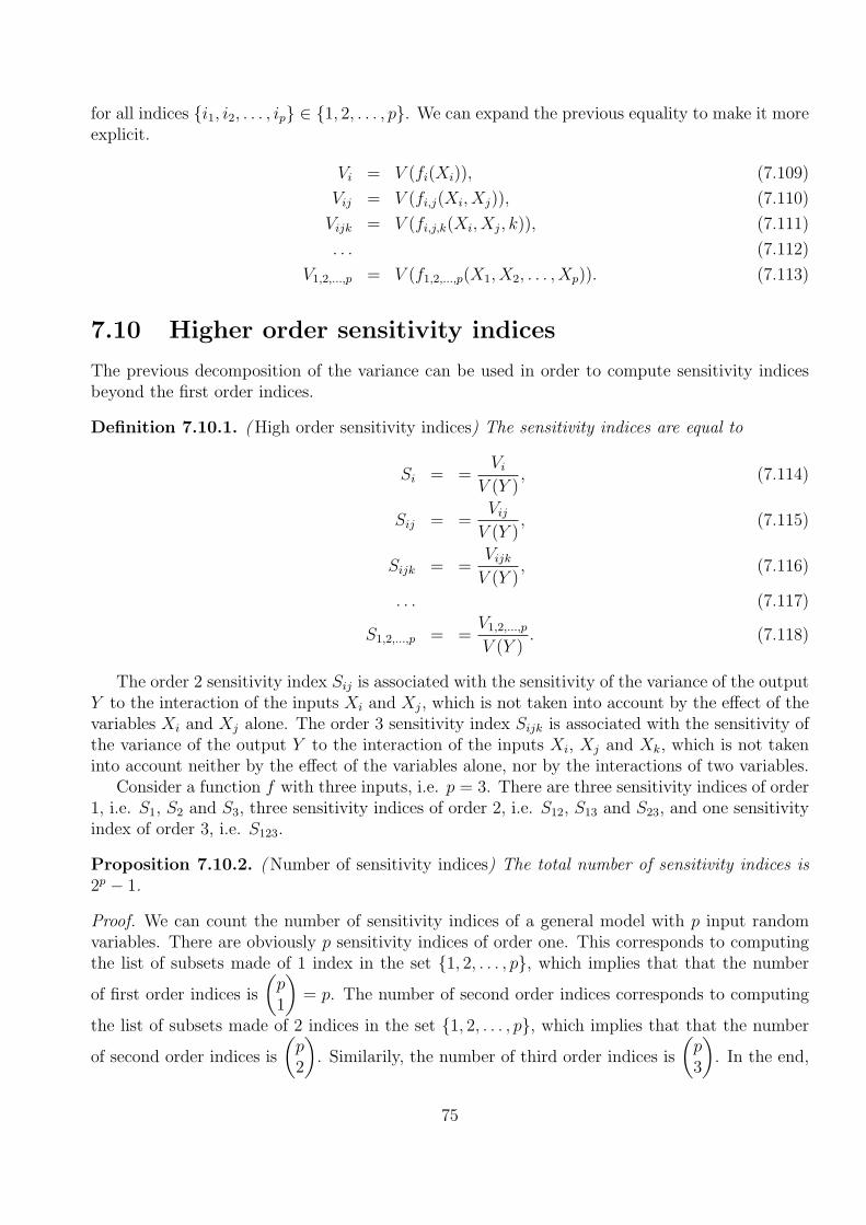
for all indices {i1, i2, . . . , ip} ∈ {1, 2, . . . , p}. We can expand the previous equality to make it moreexplicit.

Vi = V (fi(Xi)), (7.109)

Vij = V (fi,j(Xi, Xj)), (7.110)

Vijk = V (fi,j,k(Xi, Xj, k)), (7.111)

. . . (7.112)

V1,2,...,p = V (f1,2,...,p(X1, X2, . . . , Xp)). (7.113)

7.10 Higher order sensitivity indices

The previous decomposition of the variance can be used in order to compute sensitivity indicesbeyond the first order indices.

Definition 7.10.1. ( High order sensitivity indices) The sensitivity indices are equal to

Si = =Vi

V (Y ), (7.114)

Sij = =VijV (Y )

, (7.115)

Sijk = =VijkV (Y )

, (7.116)

. . . (7.117)

S1,2,...,p = =V1,2,...,p

V (Y ). (7.118)

The order 2 sensitivity index Sij is associated with the sensitivity of the variance of the outputY to the interaction of the inputs Xi and Xj, which is not taken into account by the effect of thevariables Xi and Xj alone. The order 3 sensitivity index Sijk is associated with the sensitivity ofthe variance of the output Y to the interaction of the inputs Xi, Xj and Xk, which is not takeninto account neither by the effect of the variables alone, nor by the interactions of two variables.

Consider a function f with three inputs, i.e. p = 3. There are three sensitivity indices of order1, i.e. S1, S2 and S3, three sensitivity indices of order 2, i.e. S12, S13 and S23, and one sensitivityindex of order 3, i.e. S123.

Proposition 7.10.2. ( Number of sensitivity indices) The total number of sensitivity indices is2p − 1.

Proof. We can count the number of sensitivity indices of a general model with p input randomvariables. There are obviously p sensitivity indices of order one. This corresponds to computingthe list of subsets made of 1 index in the set {1, 2, . . . , p}, which implies that that the number

of first order indices is

(p1

)= p. The number of second order indices corresponds to computing

the list of subsets made of 2 indices in the set {1, 2, . . . , p}, which implies that that the number

of second order indices is

(p2

). Similarily, the number of third order indices is

(p3

). In the end,

75

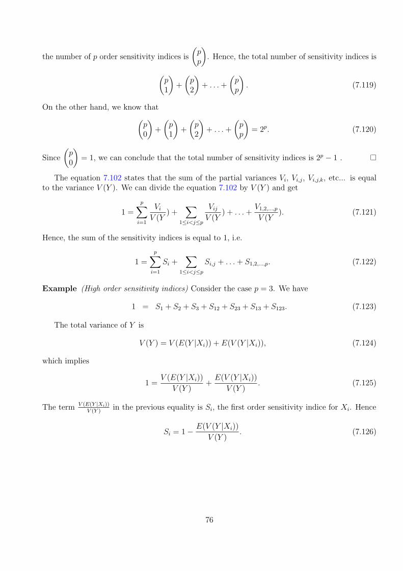
the number of p order sensitivity indices is

(pp

). Hence, the total number of sensitivity indices is

(p1

)+

(p2

)+ . . .+

(pp

). (7.119)

On the other hand, we know that(p0

)+

(p1

)+

(p2

)+ . . .+

(pp

)= 2p. (7.120)

Since

(p0

)= 1, we can conclude that the total number of sensitivity indices is 2p − 1 .

The equation 7.102 states that the sum of the partial variances Vi, Vi,j, Vi,j,k, etc... is equalto the variance V (Y ). We can divide the equation 7.102 by V (Y ) and get

1 =

p∑i=1

ViV (Y

) +∑

1≤i<j≤p

VijV (Y

) + . . .+V1,2,...,p

V (Y). (7.121)

Hence, the sum of the sensitivity indices is equal to 1, i.e.

1 =

p∑i=1

Si +∑

1≤i<j≤p

Si,j + . . .+ S1,2,...,p. (7.122)

Example (High order sensitivity indices) Consider the case p = 3. We have

1 = S1 + S2 + S3 + S12 + S23 + S13 + S123. (7.123)

The total variance of Y is

V (Y ) = V (E(Y |Xi)) + E(V (Y |Xi)), (7.124)

which implies

1 =V (E(Y |Xi))

V (Y )+E(V (Y |Xi))

V (Y ). (7.125)

The term V (E(Y |Xi))V (Y )

in the previous equality is Si, the first order sensitivity indice for Xi. Hence

Si = 1− E(V (Y |Xi))

V (Y ). (7.126)

76

7.11 Total sensitivity indices

In this section, we present the total sensitivity indices.We are interested in all the sensitivity indices Si, Sij, Sijk, etc... associated with a given

variable Xi. For example, we are interested in the sensitivity indices associated with X2, in afunction with p = 3 parameters. In this case, the associated sensitivity indices are S2, S12, S23

and S123. The associated indices are (2), (12), (23) and (123), that is, all the indices containing2.

Let us denote by Mi, the set of s-tuples (i1, i2, . . . , is) containing i, with s ≤ p. More formally,Mi is the set of s-tuples (i1, i2, . . . , is) such that i1, i2, . . . , is ∈ {1, 2, . . . , p} and there is a j ∈{1, 2, . . . , s} such that ij = i. In the previous example, we have C2 = {(2), (12), (23), (123)}.

Definition 7.11.1. ( Total sensitivity indices) For any i = 1, 2, . . . , p, the total sensitivity indexSTi with respect to the variable Xi is the sum of all the sensitivity indices associated with thevariable Xi, i.e.

STi =∑k∈Mi

Sk. (7.127)

Example (Total sensitivity indices) Consider the case p = 3. The total sensitivity index associ-ated with X2 is

ST2 = S2 + S12 + S23 + S123. (7.128)

By the equation 7.122, we have

1 = S1 + S2 + S3 + S12 + S23 + S13 + S123 (7.129)

= ST2 + S1 + S3 + S13. (7.130)

In other words, the sum of the total sensitivity index with respect to X2 and the sensitivity indicesnot containing 2 is 1. Hence,

ST2 = 1− S1 − S3 − S13. (7.131)

We can make a link between the total sensitivity indice STi and the expectation of the condi-tionnal variance of the variables different from i. We have

1 =V (E(Y |X∼i))

V (Y )+E(V (Y |X∼i))

V (Y ). (7.132)

The term E(V (Y |X∼i))V (Y )

is the total variance STi for the variable Xi. Hence,

STi = 1− V (E(Y |X∼i))V (Y )

. (7.133)

77

7.12 Ishigami function

In this section, we consider the model

Y = f(X1, X2, X3) = sin(X1) + a sin2(X2) + bX43 sin(X1) (7.134)

where X1, X2, X3 are three random variables uniform in [−π, π]. This implies that the distributionfunction of the variable Xi, fi, satisfies the equation

fi(Xi) =1

2π, (7.135)

for i = 1, 2, 3.We are going to compute the expectation, the variance and the sensitivity indices of this

function. Before this, we need auxialiary results which are presented first.

7.12.1 Elementary integration

We first notice that the integral of the sin function in the interval [−π, π] is zero, since thisfunction is symetric. Hence, ∫ π

−πsin(x)dx = 0. (7.136)

We are going to prove that ∫ π

−πsin2(x)dx = π. (7.137)

Indeed, if we integrate the sin2(x) function by part, we get∫ π

−πsin2(x)dx = [− cos(x) sin(x)]π−π −

∫ π

−π(− cos(x)) cos(x)dx (7.138)

= 0 +

∫ π

−πcos2(x)dx. (7.139)

On the other hand, the equality cos2(x) + sin2(x) = 1 implies∫ π

−πsin2(x)dx =

∫ π

−π(1− cos2(x))dx (7.140)

= 2π −∫ π

−πcos2(x)dx. (7.141)

We now combine 7.139 and 7.141 and get∫ π

−πcos2(x)dx = 2π −

∫ π

−πcos2(x)dx. (7.142)

The previous equality implies that

2

∫ π

−πcos2(x)dx = 2π, (7.143)

78

which leads to ∫ π

−πcos2(x)dx = π. (7.144)

Finally, the previous equality, combined with 7.139 immediately leads to 7.137.We are going to prove that ∫ π

−πsin4(x)dx =

3π

4. (7.145)

Indeed, if we integrate the sin4(x) function by part, we get∫ π

−πsin4(x)dx =

[− cos(x) sin3(x)

]π−π −

∫ π

−π(− cos(x))(3 sin2(x) cos(x))dx (7.146)

= 0 + 3

∫ π

−πcos2(x) sin2(x)dx. (7.147)

On the other hand, the equality cos2(x) + sin2(x) = 1 implies∫ π

−πsin4(x)dx =

∫ π

−πsin2(x) sin2(x)dx (7.148)

=

∫ π

−π(1− cos2(x)) sin2(x)dx (7.149)

=

∫ π

−πsin2(x)dx−

∫ π

−πcos2(x) sin2(x)dx. (7.150)

We plug the equality 7.137 into the previous equation and get∫ π

−πsin4(x)dx = π −

∫ π

−πcos2(x) sin2(x)dx. (7.151)

We combine 7.147 and 7.147 and get

3

∫ π

−πcos2(x) sin2(x)dx = π −

∫ π

−πcos2(x) sin2(x)dx. (7.152)

The previous equation leads to

4

∫ π

−πcos2(x) sin2(x)dx = π, (7.153)

which implies ∫ π

−πcos2(x) sin2(x)dx =

π

4, (7.154)

We finally plug the equation 7.154 into 7.147 and get the equation 7.145.

79

7.12.2 Expectation

By assumption, the three random variables X1, X2 and X3 are independent, so that the jointdistribution function is the product of the three distribution functions fi, i.e.

g1,2,3(x1, x2, x3) = g1(x1)g2(x2)g3(x3). (7.155)

By definition, the expectation of the random variable sin(X1) is

E(sin(X1)) =

∫ π

−π

∫ π

−π

∫ π

−πsin(x1)g1,2,3(x1, x2, x3)dx1dx2dx3 (7.156)

=

∫ π

−π

∫ π

−π

∫ π

−πsin(x1)g1(x1)g2(x2)g3(x3)dx1dx2dx3 (7.157)

=1

2π

∫ π

−πsin(x1)dx1 (7.158)

= 0. (7.159)

By definition, the expectation of the random variable sin2(X2) is

E(sin2(X2)) =

∫ π

−π

∫ π

−π

∫ π

−πsin2(x2)g1,2,3(x1, x2, x3)dx1dx2dx3 (7.160)

=

∫ π

−πsin2(x2)g2(x2)dx2 (7.161)

=1

2π

∫ π

−πsin2(x2)dx2. (7.162)

The equality 7.137 then implies that

E(sin2(X2)) =1

2π· π (7.163)

=1

2. (7.164)

By definition, the expectation of the random variable X43 is

E(X43 ) =

∫ π

−π

∫ π

−π

∫ π

−πx4

3g1,2,3(x1, x2, x3)dx1dx2dx3 (7.165)

=

∫ π

−π

∫ π

−π

∫ π

−πx4

3g1(x1)g2(x2)g3(x3)dx1dx2dx3 (7.166)

=

∫ π

−πx4

3g3(x3)dx3 (7.167)

=1

2π

∫ π

−πx4

3dx3, (7.168)

=1

2π

[1

5x5

3

]π−π

(7.169)

=1

2π

(1

5π5 − 1

5(−π)5

)(7.170)

=1

2π

2

5π5 (7.171)

=1

5π4. (7.172)

80

We are now going to use the expectations 7.159, 7.164 and 7.172 in order to compute theexpectation of the output Y . The model 7.134 is a sum of functions. Since the expectation ofa sum of two random variables is the sum of the expectations (be the variables independent ornot), we have

E(Y ) = E(sin(X1)) + E(a sin2(X1)) + E(bX43 sin(X1)) (7.173)

= E(sin(X1)) + aE(sin2(X1)) + bE(X43 sin(X1)). (7.174)

The expectation of the variable X43 sin(X1) is

E(X43 sin(X1)) =

∫ π

−π

∫ π

−π

∫ π

−π(x4

3 sin(x1))g1,2,3(x1, x2, x3)dx1dx2dx3 (7.175)

=

∫ π

−π

∫ π

−π

∫ π

−π(x4

3 sin(x1))g1(x1)g2(x2)g3(x3)dx1dx2dx3 (7.176)

= E(X43 )E(sin(X1)). (7.177)

Hence, the expectation of Y is

E(Y ) = E(sin(X1)) + aE(sin2(X1)) + bE(X43 )E(sin(X1)). (7.178)

We now combine the equations 7.159, 7.164 and 7.172 and get

E(Y ) = 0 + a1

2+ b

1

5π4 · 0 (7.179)

=a

2. (7.180)

7.12.3 Variance

The variance of the output Y is

V (Y ) = E(Y 2)− E(Y )2 (7.181)

= E((

sin(X1) + a sin2(X2) + bX43 sin(X1)

)2)− E(Y )2 (7.182)

= E(sin2(X1) + a2 sin4(X2) + b2X8

3 sin2(X1)+ (7.183)

2 sin(X1)a sin2(X2) + 2 sin2(X1)bX43+ (7.184)

2a sin2(X2)bX43 sin(X1)

)− E(Y )2 (7.185)

= E(sin2(X1)) + a2E(sin4(X2)) + b2E(X83 )E(sin2(X1)) + (7.186)

2aE(sin(X1))E(sin2(X2)) + 2bE(sin2(X1))E(X43 ) + (7.187)

2abE(sin2(X2))E(X43 )E(sin(X1))− E(Y )2. (7.188)

By the equality 7.159, the expectation of sin(X1) is zero in the interval [−π, π]. Therefore, theterms associated with E(sin(X1)) can be simplified in the previous equality. This leads to

V (Y ) = E(sin2(X1)) + a2E(sin4(X2)) + b2E(X83 )E(sin2(X1)) + (7.189)

2bE(X43 )E(sin2(X1))− E(Y )2 (7.190)

81

We now compute the terms appearing in the previous equality. Actually, we do not have muchto compute, since the equalities 7.164 and 7.172 are already available. Indeed, the equality 7.164immediately leads to

E(sin2(X1)) = E(sin2(X2)) (7.191)

=1

2. (7.192)

What remains to compute is E(sin4(X2)) and E(X83 ).

By definition, the expectation of the random variable X43 is

E(X83 ) =

1

2π

∫ π

−πx8

3dx3, (7.193)

=1

2π

[1

9x9

3

]π−π

(7.194)

=1

2π

(1

9π9 − 1

9(−π)9

)(7.195)

=1

2π

2

9π9 (7.196)

=1

9π8. (7.197)

On the other hand, the expectation of the random variable sin4(X2) is

E(sin2(X2)) =1

2π

∫ π

−πsin4(x2)dx2. (7.198)

The equality 7.145 then implies that

E(sin4(X2)) =1

2π· 3π

4(7.199)

=3

8. (7.200)

We now plug the equalities 7.192, 7.172, 7.197 and 7.200 into 7.190, and get

V (Y ) =1

2+ a2 3

8+ b2

1

9π8 1

2+ 2b

1

5π4 1

2− a2

22(7.201)

=1

2+

3a2

8+b2π8

18+bπ4

5− a2

4(7.202)

=1

2+a2

8+b2π8

18+bπ4

5(7.203)

7.12.4 Sobol decomposition

In this section, we perform the Sobol decompotion of the function f , as presented in the section7.7.


f0 = E(Y ) (7.204)

=a

2. (7.205)

82

We are first interested in the first order decomposition functions f1, f2 and f3 and theirassociated variances V1, V2 and V3.


f1(X1) = −f0 +

∫ 1

0

∫ 1

0

f(x)dx∼1 (7.206)

= −a2

+

∫ 1

0

∫ 1

0

f(x)dx2dx3 (7.207)

= −a2

+

∫ 1

0

∫ 1

0

(sin(X1) + a sin2(x2) + bx4

3 sin(X1))dx2dx3 (7.208)

= −a2

+ sin(X1) + aE(sin2(X2)) + bE(x43) sin(X1) (7.209)

= −a2

+ sin(X1) + a1

2+ bE(X4

3 ) sin(X1) (7.210)

= −a2

+ sin(X1) + a1

2+ b

π4

5sin(X1) (7.211)

= sin(X1)

(1 + b

π4

5

). (7.212)

The variance of f1 is

V1 = V (f1(X1)) (7.213)

= E(f1(X1)2)− E(f1(X1))

2. (7.214)

But the equality 7.67 states that the integral of any function fi with respect to its arguments iszero. Hence E(f1(X1)) = 0. This implies

V1 = E(f1(X1)2) (7.215)

= E

((sin(x1)

(1 + b

π4

5

))2)

(7.216)

= E(sin2(x1))

(1 + b

π4

5

)(7.217)

=1

2

(1 + b

π4

5

)2

. (7.218)

Similarily, we have

f2(X2) = −f0 +

∫ 1

0

∫ 1

0

f(x)dx∼2 (7.219)

= −a2

+

∫ 1

0

∫ 1

0

f(x)dx1dx3 (7.220)

= −a2

+ E(sin(X1)) + a sin2(X2) + bE(X43 )E(sin(X1)) (7.221)

= −a2

+ a sin2(X2). (7.222)

83

Hence,

V2 = E(f2(X2)2) (7.223)

= E((−a2

+ a sin2(X2))2) (7.224)

= E(a2

4+ a2 sin4(X2)− a2 sin2(X2)) (7.225)

=a2

4+ a2E(sin4(X2))− a2E(sin2(X2)) (7.226)

=a2

4+

3

8a2 − a2

2(7.227)

=a2

8. (7.228)

Similarily, we have

f3(X3) = −f0 +

∫ 1

0

∫ 1

0

f(x)dx∼3 (7.229)

= −a2

+

∫ 1

0

∫ 1

0

f(x)dx1dx2 (7.230)

= −a2

+ E(sin(X1)) + aE(sin2(X2)) + bX3E(sin(X1)) (7.231)

= −a2

+a

2(7.232)

= 0. (7.233)

Hence,

V3 = E(f3(X3)2) (7.234)

= 0. (7.235)

We can immediately conclude that S3 is zero. The fact that S3 is zero illustrates the fact thatconditional variances may be difficult to analyze. Indeed, the equation S3 = 0 implies that thefraction of the variance that can be explained by the effect of X3 alone is zero. It does not implythat the variable X3 has no effect: X3 as an effect, when we consider its interaction with X1,because of the b sin(X1) term.

We are now interested in the second order decomposition functions f1,2, f1,3 and f2,3.

84

We have

f1,2(X1, X2) = −f0 − f1(X1)− f2(X2) +

∫ 1

0

f(x)dx∼1,2 (7.236)

= −f0 − f1(X1)− f2(X2) +

∫ 1

0

f(x)dx3 (7.237)

= −a2− sin(X1)

(1 + b

π4

5

)+a

2− a sin2(X2) + (7.238)

sin(X1) + a sin2(X2) + bE(X43 ) sin(X1) (7.239)

= − sin(X1)

(1 + b

π4

5

)− a sin2(X2) + (7.240)

sin(X1) + a sin2(X2) + bπ4

5sin(X1) (7.241)

= 0. (7.242)

Hence,

V1,2 = V (f1,2(X1, X2)) (7.243)

= 0. (7.244)

We can immediately conclude that S1,2 is zero. This can be predicted from the equation 7.134,since there is no interaction between the variables X1 and X2.

We have

f1,3(X1, X3) = −f0 − f1(X1)− f3(X3) +

∫ 1

0

f(x)dx∼1,3 (7.245)

= −f0 − f1(X1)− f3(X3) +

∫ 1

0

f(x)dx2 (7.246)

= −a2− sin(X1)

(1 + b

π4

5

)+ (7.247)

sin(X1) + aE(sin2(X2)) + bX43 sin(X1) (7.248)

= −a2− sin(X1)

(1 + b

π4

5

)+ sin(X1) +

a

2+ bX4

3 sin(X1) (7.249)

= − sin(X1)bπ4

5+ bX4

3 sin(X1) (7.250)

= b sin(X1)

(X4

3 −π4

5

). (7.251)

Hence,

V1,3 = V (f1,3(X1, X3)) (7.252)

= E(f1,3(X1, X3)2)− E(f1,3(X1, X3))

2 (7.253)

85

The equality 7.67 implies that E(f1,3(X1, X3)) = 0. Hence,

V1,3 = E(f1,3(X1, X3)2) (7.254)

= b2E(sin2(X1))E

((X4

3 −π4

5

)2)

(7.255)

=b2

2E(X8

3 +π8

25− 2X4

3

π4

5) (7.256)

=b2

2(E(X8

3 ) +π8

25− 2E(X4

3 )π4

5) (7.257)

=b2

2(π8

9+π8

25− 2

π4

5

π4

5) (7.258)

=b2

2(π8

9+π8

25− 2

π8

25) (7.259)

=b2

2(π8

9− π8

25) (7.260)

=b2π8

2(1

9− 1

25). (7.261)

We have

f2,3(X2, X3) = −f0 − f2(X2)− f3(X3) +

∫ 1

0

f(x)dx∼2,3 (7.262)

= −f0 − f2(X2)− f3(X3) +

∫ 1

0

f(x)dx1 (7.263)

= −a2−(−a

2+ a sin2(X2)

)− 0 + (7.264)

E(sin(X1)) + a sin2(x2) + bx43E(sin(X1)) (7.265)

= 0. (7.266)

Hence,

V2,3 = 0. (7.267)

Finally, we can compute the function f1,2,3 and the variance V1,2,3. We have

f1,2,3(X1, X2, X3) = −f0 − f1(X1)− f2(X2)− f3(X3)− f1,2(X1, X2) (7.268)

−f1,3(X1, X3)− f2,3(X2, X3) + f(X1, X2, X3) (7.269)

= 0. (7.270)

Hence

V1,2,3 = 0. (7.271)

7.12.5 Summary of the results

In this section, we present a summary of the results for the Ishigami function

Y = f(X1, X2, X3) = sin(X1) + a sin2(X2) + bX43 sin(X1) (7.272)

86

where X1, X2, X3 are three random variables uniform in [−π, π]. The expectation and the varianceof Y are

E(Y ) =a

2(7.273)

V (Y ) =1

2+a2

8+b2π8

18+bπ4

5(7.274)

The Sobol decomposition functions are

f0 =a

2(7.275)

f1(X1) = sin(X1)

(1 + b

π4

5

)(7.276)

f2(X2) = −a2

+ a sin2(X2) (7.277)

f3(X3) = 0 (7.278)

f1,2(X1, X2) = 0 (7.279)

f1,3(X1, X3) = b sin(X1)

(X4

3 −π4

5

)(7.280)

f2,3(X2, X3) = 0 (7.281)

f1,2,3(X1, X2, X3) = 0. (7.282)

The Sobol decomposition variances are

V1 =1

2

(1 + b

π4

5

)2

(7.283)

V2 =a2

8(7.284)

V3 = 0 (7.285)

V1,2 = 0 (7.286)

V1,3 =b2π8

2(1

9− 1

25) (7.287)

V2,3 = 0 (7.288)

V1,2,3 = 0. (7.289)

7.12.6 Numerical results

In this section, we present numerical results associated with the Ishigami function.We begin by defining the Ishigami function.

function y = ishigami (x)a=7.b=0.1s1=sin(x(:,1))s2=sin(x(:,2))x34 = x(: ,3).^4y(:,1) = s1 + a.*s2.^2 + b.*x34.*s1

endfunction

87

In the following script, we perform a Monte-Carlo sampling and compute the output of theIshigami function. Then we plot the output Y against its input arguments X1, X2 and X3.

np = 1000;A = grand(np ,3,"def")*2* %pi - %pi;y = ishigami (A);scf();subplot (1,3,1);plot(A(:,1),y,"bo")xtitle("","X1","f(X1,X2,X3)");subplot (1,3,2);plot(A(:,2),y,"bo")xtitle("","X2","f(X1,X2,X3)");subplot (1,3,3);plot(A(:,3),y,"bo")xtitle("","X3","f(X1,X2,X3)");// Put the marks as transparenth.children (1). children.children.mark_background = 0;h.children (2). children.children.mark_background = 0;h.children (3). children.children.mark_background = 0;


Figure 7.8: Output of the Ishigami function with respect to each input argument.

The following function returns the exact expectation, variance and sensitivity indices of theIghigami function.

function exact = ishigami_saexact ( a , b )// Exact results for the Ishigami functionexact.expectation = a/2;exact.var = 1/2 + a^2/8 + b*%pi ^4/5 + b^2*%pi ^8/18;// Sensitivity indices.exact.S1 = (1/2 + b*%pi ^4/5+b^2*%pi ^8/50)/ exact.var;exact.S2 = (a^2/8)/ exact.var;exact.S3 = 0;exact.S12 = 0;exact.S23 = 0;exact.S13 = b^2*%pi ^8/2*(1/9 -1/25)/ exact.var;exact.S123 = 0;

88

exact.ST1 = exact.S1 + exact.S12 + exact.S13 + exact.S123;exact.ST2 = exact.S2 + exact.S12 + exact.S23 + exact.S123;exact.ST3 = exact.S3 + exact.S13 + exact.S23 + exact.S123;

endfunction

The following script allows to get the results associated with the parameters a = 7 and b = 0.1.

a=7.;b=0.1;exact = ishigami_saexact ( a , b )


-->exact = ishigami_saexact ( a , b )exact =

expectation: 3.5var: 13.844588S1: 0.3139052S2: 0.4424111S3: 0S12: 0S23: 0S13: 0.2436837S123: 0ST1: 0.5575889ST2: 0.4424111ST3: 0.2436837

7.13 A straightforward approach

In this section, we present a straightforward approach for the computation of the first ordersensitivity indices. As we are going to see, this method requires a too large number of functionevaluations. This section then motivate the need for more elaborate algorithms which are goingto be presented in the remaining sections.

Let us compute the sensitivity indice associated with a uniform random variable Xi, for i =1, 2, . . . , p. The analysis is based on the decomposition of the input variables of the function f

f(X) = f(Xi, X∼i), (7.290)

where the indices ∼ i are all the integers different from i. By the equation 7.103, we have

Vi = V (E(Y |Xi)). (7.291)

We could employ a straightforward method to estimate the previous variance, based on twonested loops. Indeed, we can set the variable Xi to a particular value, say Xj. From there, wecan create a sampling for the remaining parameters X∼i, based on n Monte-Carlo simulations,where n is a relatively large integer, say n = 1000. This leads to the experiments

yk |Xi=Xj= f(xk1, x

k2, . . . , Xi, . . . , x

kp), (7.292)

89

for k = 1, 2, . . . , n. Once done, we have a set of values {yk|Xi = Xk}k=1,2,...,n and can computethe associated expectation

E(Y |Xi = Xj) =1

n

∑k=1,2,...,n

yk |Xi=Xj. (7.293)

We can repeat this experiment m times, so that we now have the set of expectations E(Y |Xi = Xj)for j = 1, 2, . . . ,m. We can then compute the expectation and the variance of this randomvariable, with

E(Y ) =1

m

∑j=1,2,...,n

E(Y |Xi = Xj) (7.294)

Vi =1

m− 1

∑j=1,2,...,m

(E(Y |Xi = Xj)− E(Y ))2. (7.295)

This method requires a total of n ·m evaluations of f , which is too large to be manageablein practice. For example, if n =1 000 and m =1 000, the previous method requires 1 000000 function evaluations. Given the accuracy of Monte-Carlo experiments, the result would beunusable in practical cases.

7.14 The Sobol method for sensitivity analysis

In this section, we present a method by Sobol [10] to estimate the sensitivity indices, usingMonte-Carlo experiments.

Let us compute the sensitivity indice associated with a uniform random variable Xi, for i =1, 2, . . . , p. The analysis is based on the decomposition of the input variables of the function f

f(X) = f(Xi, X∼i), (7.296)

where the indices ∼ i are all the integers different from i. By the equation 7.103, we have

Vi = V (E(Y |Xi)). (7.297)

By the definition of a variance,

Vi = E(E(Y |Xi)2)− E(E(Y |Xi))

2. (7.298)

We can begin by computing the expression E(E(Y |Xi))2. By the definition of the conditionnal

expectation,

E(Y |Xi) =

∫f(Xi, X∼i)dX∼i, (7.299)

so that

E(E(Y |Xi)) =

∫ (∫f(Xi, X∼i)dX∼i

)dXi (7.300)

=

∫f(X)dX (7.301)

= E(Y ). (7.302)

90

Hence,

Vi = E(E(Y |Xi)2)− E(Y )2. (7.303)

On the other hand,

E(E(Y |Xi)2) = E

((∫f(Xi, X∼i)dX∼i

)2)

(7.304)

=

∫ (∫f(Xi, X∼i)dX∼i

)2

dXi (7.305)

=

∫ ∫ ∫f(Xi, X∼i)f(Xi, Z∼i)dX∼idZ∼idXi. (7.306)

We plug the previous equation into 7.298 and get

Vi =

∫ ∫ ∫f(Xi, X∼i)f(Xi, Z∼i)dX∼idZ∼idXi.− E(Y )2. (7.307)

Remark 7.14.1. Although the two previous computations seem monstruous at first, they aresimply derived from the basic following result. Assume that g is a smooth integrable function ofone variable x ∈ [0, 1]. Then, we have the following elementary result:(∫

g(x)dx

)2

=

(∫g(x)dx

)(∫g(x)dx

)(7.308)

=

(∫g(x)dx

)(∫g(y)dy

)(7.309)

=

(∫ (∫g(x)dx

)g(y)dy

)(7.310)

=

∫ ∫g(x)g(y)dxdy. (7.311)

Hence, the move from the equation 7.305 to 7.306 is just the application of the previous resultapplied to the function g(X∼i) = f(Xi, Z∼i), i.e. considering the variables X∼i.

In [8], Saltelli notices that the equation 7.306 is the expected value of the function F of 2p− 1variables:

F (Xi, X∼i, Z∼i) = f(Xi, X∼i)f(Xi, Z∼i). (7.312)

Hence, the integral 7.306 can be evaluated using a single Monte-Carlo loop.The following method is due to Sobol, Homma and Saltelli. It is based on the use of two

sampling A and B, made of n experiments:

A =

xA,11 xA,12 . . . xA,1p

xA,21 xA,22 . . . xA,2p...

......

xA,n1 xA,n2 . . . xA,np

, B =

xB,11 xB,12 . . . xB,1p

xB,21 xB,22 . . . xB,2p...

......

xB,n1 xB,n2 . . . xB,np

. (7.313)

91

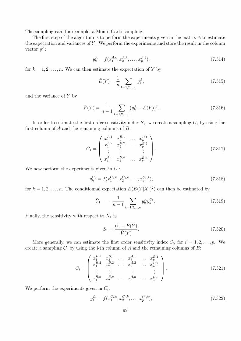
The sampling can, for example, a Monte-Carlo sampling.The first step of the algorithm is to perform the experiments given in the matrix A to estimate

the expectation and variances of Y . We perform the experiments and store the result in the columnvector yA:

yAk = f(xA,k1 , xA,k2 , . . . , xA,kp ), (7.314)

for k = 1, 2, . . . , n. We can then estimate the expectation of Y by

E(Y ) =1

n

∑k=1,2,...,n

yAk , (7.315)

and the variance of Y by

V (Y ) =1

n− 1

∑k=1,2,...,n

(yAk − E(Y ))2. (7.316)

In order to estimate the first order sensitivity index S1, we create a sampling C1 by using thefirst column of A and the remaining columns of B:

C1 =

xA,11 xB,12 . . . xB,1p

xA,21 xB,22 . . . xB,2p...

......

xA,n1 xB,n2 . . . xB,np

. (7.317)

We now perform the experiments given in C1:

yC1k = f(xC1,k

1 , xC1,k2 , . . . , xC1,k

p ), (7.318)

for k = 1, 2, . . . , n. The conditionnal expectation E(E(Y |X1)2) can then be estimated by

U1 =1

n− 1

∑k=1,2,...,n

yAk yC1k . (7.319)

Finally, the sensitivity with respect to X1 is

S1 =U1 − E(Y )

V (Y ). (7.320)

More generally, we can estimate the first order sensitivity index Si, for i = 1, 2, . . . , p. Wecreate a sampling Ci by using the i-th column of A and the remaining columns of B:

Ci =

xB,11 xB,12 . . . xA,1i . . . xB,1p

xB,21 xB,22 . . . xA,2i . . . xB,2p...

......

...

xB,n1 xB,n2 . . . xA,ni . . . xB,np

. (7.321)

We perform the experiments given in Ci:

yCik = f(xCi,k

1 , xCi,k2 , . . . , xCi,k

p ), (7.322)

92

for k = 1, 2, . . . , n. The conditionnal expectation E(E(Y |Xi)2) can then be estimated by

Ui =1

n− 1

∑k=1,2,...,n

yAk yCik . (7.323)

Finally, the sensitivity with respect to Xi is

Si =Ui − E(Y )2

V (Y ). (7.324)

The initial A sampling requires n function evaluations, which allows to compute the expecta-tion and the variance. From there, each sensitivity indice Si requires n function evaluations. Allthe first order sensitivity indices can therefore be approximated with n+ pn function evaluations.

The same procedure can be used to estimate the higher sensitivity indices. For example, inorder to compute the second order sensitivity indice Si,j, we use the sampling

Ci,j =

xB,11 xB,12 . . . xA,1i . . . xA,1j . . . xB,1p

xB,21 xB,22 . . . xA,2i . . . xA,1j . . . xB,2p...

......

......

xB,n1 xB,n2 . . . xA,ni . . . xA,1j . . . xB,np

. (7.325)

We perform the experiments given in Ci:

yCi,j

k = f(xCi,j ,k1 , x

Ci,j ,k2 , . . . , xCi,j ,k

p ), (7.326)

for k = 1, 2, . . . , n. The conditionnal expectation E(E(Y |Xi, Xj)2) can then be estimated by

Ui,j =1

n− 1

∑k=1,2,...,n

yAk yCi,j

k . (7.327)

Finally, the sensitivity with respect to Xi and Xj is

Si,j =Ui,j − E(Y )

V (Y )− Si − Sj. (7.328)

The procedure can be used to estimate the total sensitivity indices STi, for i = 1, 2, . . . , p. Welearnt in the section 7.11 that

STi = 1− V (E(Y |X∼i))V (Y )

. (7.329)

We then have to approximate

V∼i = V (E(Y |X∼i)) (7.330)

= E(E(Y |X∼i)2)− E(E(Y |X∼i))2 (7.331)

= E(E(Y |X∼i)2)− E(Y )2. (7.332)

Therefore, we have to compute

U∼i = E(E(Y |X∼i)2). (7.333)

93

We perform the experiments from the B sampling and store the result in the column vector yB:

yBk = f(xB,k1 , xB,k2 , . . . , xB,kp ), (7.334)

for k = 1, 2, . . . , n. Notice that the difference between the matrices B and Ci, only the column ichanges. We finally approximate U∼i by

U∼i =1

n− 1

∑k=1,2,...,n

yBk yCik . (7.335)

The equation 7.323 for the computation of Ui is discussed in [9], Chapter 5. ”Methods basedon decomposing the variance of the output”, section 5.9. We can think of A as the ”sample”matrix and of B as the ”resample” matrix. The term Ui is obtained from the product of values off computed from the sample matrix times values of f computed from Ci, i.e. a matrix where allfactors except Xi are re-sampled.

• If Xi is an influential factor, then high values of yAk will be preferentially associated withhigh values of yCi

k .

• If Xi is the only influential factor (all the others being dummies), then the two values of fwill be identical.

• If Xi is a totally non-influential factor, then high and low values of yAk will be randomlyassociated with high and low values of yCi

k .

Therefore, the estimate Ui of the sensitivity of Xi must be larger for an influential factor Xi thanfor a non-influential one.

TODO : the accuracy issue of the varianceTODO : why using the covariance instead of the difference formula for uiTODO : the comment of Saltelli of another formula for ui in the case of a non-influential factor

7.15 The Ishigami function by the Sobol method

In this section, we compute the sensitivity indices of the Ishigami function by the Sobol method.We consider three random variables uniform in [−π, π]. We use Monte-Carlo experiments tocompute the sensitivity indices.

The following function allows to compute the covariance matrix of its two input arguments xand y.

function C = nisp_cov ( x , y )x=x(:)y=y(:)n = size(x,"*")x=x-mean(x)y=y-mean(y)C(1,1) = x’*x/(n-1)C(1,2) = x’*y/(n-1)C(2,1) = C(1,2)C(2,2) = y’*y/(n-1)

endfunction

94

The following function returns the sensitivity index associated with the experiments ya andyc.

function s = sensitivityindex(ya,yc)// Returns the sensitivity index// associated with experiments ya and yc.C = nisp_cov (ya, yc)s= C(1,2)/ (st_deviation(ya) * st_deviation(yc))

endfunction

The following script allows to perform the analysis.

// Create the uncertain parametersrvu1 = randvar_new("Uniforme",-%pi ,%pi);rvu2 = randvar_new("Uniforme",-%pi ,%pi);rvu3 = randvar_new("Uniforme",-%pi ,%pi);srvu = setrandvar_new ();setrandvar_addrandvar ( srvu , rvu1);setrandvar_addrandvar ( srvu , rvu2);setrandvar_addrandvar ( srvu , rvu3);// The number of uncertain parameters is :nx = setrandvar_getdimension(srvu);np = 10000;// Create a first sampling Asetrandvar_buildsample(srvu ,"Lhs",np);A = setrandvar_getsample(srvu);// Create a first sampling Bsetrandvar_buildsample(srvu ,"Lhs",np);B = setrandvar_getsample(srvu);// Perform the experiments in Aya = ishigami(A);// Compute the first order sensitivity index for X1C = B;C(1:np ,1)=A(1:np ,1);yc = ishigami(C);s1 = sensitivityindex(ya,yc);mprintf("S1 : %f (expected = %f)\n", s1, exact.S1);// Compute the first order sensitivity index for X2C = B;C(1:np ,2)=A(1:np ,2);yc = ishigami(C);s2 = sensitivityindex(ya,yc);mprintf("S2 : %f (expected = %f)\n", s2, exact.S2);// Compute the first order sensitivity index for X3C = B;C(1:np ,3)=A(1:np ,3);yc = ishigami(C);s3 = sensitivityindex(ya,yc);mprintf("S3 : %f (expected = %f)\n", s3, exact.S3);// Compute the first order sensitivity index for {X1 ,X3}C = A;

95

C(1:np ,2)=B(1:np ,2);yc = ishigami(C);s13 = sensitivityindex(ya,yc)-s1-s3;mprintf("S13 : %f (expected = %f)\n", s13 , exact.S13);// Compute the sensitivity index for {X2,X3}C = B;C(:,[2 3])=A(:,[2 3]);yc = ishigami(C);s23 = sensitivityindex(ya,yc)-s2-s3;mprintf("S23 : %f (expected = %f)\n", s23 , exact.S23);// Compute the sensitivity index for {X1,X2,X3}C = B;C(:,[1 2 3])=A(:,[1 2 3]);yc = ishigami(C);s123 = sensitivityindex(ya,yc)-s1-s2-s3-s12 -s23 -s13;mprintf("S123 : %f (expected = %f)\n", s123 , exact.S123);// Compute the total sensitivity index for X1C = A;C(:,1)=B(:,1);yc = ishigami(C);st1 = 1-sensitivityindex(ya ,yc);mprintf("ST1 : %f (expected = %f)\n", st1 , exact.ST1);// Compute the total sensitivity index for X2C = A;C(:,2)=B(:,2);yc = ishigami(C);st2 = 1-sensitivityindex(ya ,yc);mprintf("ST2 : %f (expected = %f)\n", st2 , exact.ST2);// Compute the total sensitivity index for X3C = A;C(:,3)=B(:,3);yc = ishigami(C);st3 = 1-sensitivityindex(ya ,yc);mprintf("ST3 : %f (expected = %f)\n", st3 , exact.ST3);//// Clean -uprandvar_destroy(rvu1);randvar_destroy(rvu2);randvar_destroy(rvu3);setrandvar_destroy(srvu);


S1 : 0.311242 (expected = 0.313905)S2 : 0.449588 (expected = 0.442411)S3 : 0.000827 (expected = 0.000000)S12 : -0.006056 (expected = 0.000000)S13 : 0.245094 (expected = 0.243684)S23 : -0.008243 (expected = 0.000000)S123 : 0.007548 (expected = 0.000000)

96

ST1 : 0.557828 (expected = 0.557589)ST2 : 0.442837 (expected = 0.442411)ST3 : 0.245226 (expected = 0.243684)

In the following script, we create the histogram of the output of the Ishigami function.

scf();histplot (50,ya)xtitle("Ishigami function","X","P(X)")


0.00

0.02

0.04

0.06

0.08

0.10

0.12

-10 -5 0 5 10 15 20

Ishigami function

X

P(X

)

Figure 7.9: Histogram of the output of the Ishigami function.

7.16 Notes and references

More details on this topic can be found in the papers of Homma and Saltelli [4] or in the work ofSobol [10].

The thesis by Jacques [6] presents an overview of sensitivity analysis. Some of the resultspresented here are extracted from the short introduction by Jacques [5].

The book by Saltelli, Tanrantola, Compolongo and Ratto [9] presnts a description of a fewselected techniques for sensitivity analysis. Their presentation is based on the Simlab software,a free development framework for sensitivity analysis and uncertainty analysis. The licence ofSimlab is free for non-commercial purposes.

The first figure of this chapter is taken from the slides by Antoniadis [1].

97

Chapter 8

Thanks

Many thanks to Allan Cornet.

98

Bibliography

[1] Anestis Antoniadis. Analyse de l’incertitude et analyse de sensibilite - l’analyse de sensibilite,June 2005. Ecole d’ete CEA-EDF-INRIA.

[2] Michael Baudin. Programming in scilab, 2010.

[3] Michael Baudin and Jean-Marc Martinez. Polynomes de chaos sous scilab via la librairienisp. In 42emes Journees de Statistique, 24 au 28 mai 2010 - Marseille, France, 2010.

[4] T. Homma and A. Saltelli. Importance measures in global sensitivity analysis of non linearmodels. Reliability Engineering and System Safety, 52:1–17, 1996.

[5] Julien Jacques. Analyse de sensibilite globale, 2005. http://math.univ-lille1.fr/

~jacques/.

[6] Julien Jacques. Contributions a l’analyse de sensibilite et a l’analyse discriminante general-isee, 2005.

[7] Didier Pelat. Bases et methodes pour le traitement des donnees (Bruits et Signaux). MasterM2 Recherche : Astronomie?astrophysique, 2006.

[8] Andrea Saltelli. Making best use of model evaluations to compute sensitivity indices. Com-puter Physics Communications, 145(2):280 – 297, 2002.

[9] Andrea Saltelli, Stefano Tarantola, Francesca Compolongo, and Marco Ratto. Sensitivityanalysis in practice. John Wiley and Sons, 2004.

[10] I.M. Sobol. Sensitivity estimates for nonlinear mathematical models. Mathematical Modellingand Computational Experiments, 1:407?–414, 2003.

99

http://math.univ-lille1.fr/~jacques/

http://math.univ-lille1.fr/~jacques/

NISP Toolbox Manual - Scilabforge.scilab.org/upload/nisp/files/nisp_toolbox_manual_v... ·...

Documents

Transcript of NISP Toolbox Manual - Scilabforge.scilab.org/upload/nisp/files/nisp_toolbox_manual_v... ·...