repositorio.ul.ptrepositorio.ul.pt/bitstream/10451/33931/1/ulfc124388_tm_António... ·...
133
2018 UNIVERSIDADE DE LISBOA FACULDADE DE CIÊNCIAS DEPARTAMENTO DE FÍSICA Biomechanical Analysis of Walking in Subjects Affected by Neurological Diseases António Duarte Robalo Gonçalves Mendonça Mestrado Integrado em Engenharia Biomédica e Biofísica Perfil em Engenharia Clínica e Instrumentação Médica Dissertação orientada por: Pedro Cavaleiro Miranda Nevio Luigi Tagliamonte
Transcript of repositorio.ul.ptrepositorio.ul.pt/bitstream/10451/33931/1/ulfc124388_tm_António... ·...

2018
UNIVERSIDADE DE LISBOA
FACULDADE DE CIÊNCIAS
DEPARTAMENTO DE FÍSICA
Biomechanical Analysis of Walking in Subjects Affected by
Neurological Diseases
António Duarte Robalo Gonçalves Mendonça
Mestrado Integrado em Engenharia Biomédica e Biofísica
Perfil em Engenharia Clínica e Instrumentação Médica
Dissertação orientada por:
Pedro Cavaleiro Miranda
Nevio Luigi Tagliamonte

Acknowledgments António Mendonça 2018
II
ACKNOWLEDGEMENTS
This dissertation is dedicated to all my loving family, specially to my parents, Lucia Robalo and
João Mendonça, and to my brother, José Mendonça. Thank you for making me believe in myself,
without you, none of this would be possible. I also want to thank to my uncle, Lionel dos Santos, and
my cousin, Tomás dos Santos, for granting me access to their office to write this dissertation.
I want to express my deep gratitude to Professor Pedro Miranda, for all orientation given
throughout this dissertation, and to Eng. Nevio Tagliamonte, not only for all the guidance, but also for
the opportunity to work in such a stimulating working environment.
Thanks to Alessandro Ranieri for all orientation and advice given during the primary stages of
the internship.
I’m also extremely thankful to Dr. Marco Molinari, not only for allowing my stay at Fondazione
Santa Lucia to be possible, but also for all the help and availability. Also, from Fondazione Santa Lucia,
big thanks to Federica Tamburella, the physiotherapist that had the kindness to provide me the clinical
profiles of both healthy subjects and patients, and whose help was very important for the concretization
of this dissertation.
Regarding the work elaborated in Fondazione Santa Lucia, I must thank Matteo Arquilla, who
helped me a lot, especially during the early stages of this work’s development. I also want to express
my gratitude to Iolanda Pisotta for all the kindness and orientation inside the institution’s environment.
Again, I would like to express my deep gratitude to my loving parents for providing me the
economic support to develop my dissertation abroad.
Last, but not the least, I want to thank to my friends, for all the help and emotional support.

Abstract António Mendonça 2018
III
ABSTRACT
The occurrence of a spinal cord injury due to a motor vehicle accident, a fall, a shallow diving,
an act of violence, or a sport injury can drastically change anyone’s life. The autonomy to perform daily
life tasks, like walking, which most people take for granted, is drastically reduced, as well as one’s
quality of life. Fortunately, the use of robotic assisted rehabilitation devices can help in overcoming,
faster and more efficiently, the problems a spinal cord injury patient must face every day during the gait
performance. However, there is still a lack of clinical evidence proving that the use of such devices
provides better results than the ones provided by conventional physiotherapy, since there aren’t
standardized protocols and specific medical guidelines for using this kind of robotic systems.
This dissertation aims to enhance the human understanding about the analysis of the features of
EMG curves during the use of different robotic devices in single-shot tests. To achieve such purpose,
the gait performance of both healthy subjects and patients was tracked and analyzed, while they were
using one of the two robotic assisted rehabilitation devices: Lokomat exoskeleton or Gait Trainer GT1.
To evaluate the impact that these devices can have on the muscular activation, the electrical activity of
the tibialis anterior, soleus, gastrocnemius, biceps femoris, rectus femoris and semitendinosus, of both
right and left legs, was recorded using surface electromyography.
The experimental procedure adopted for healthy subjects was different from the one adopted for
patients. Ten healthy subjects performed five walking conditions, two of which were performed freely
over-ground and three using a robotic assisted rehabilitation device. In the context of this dissertation, a
self-paced over-ground walking condition was used as control. Ten patients performed three walking
conditions, using a robotic assisted rehabilitation device.
In a first instance, EMG data referring to both healthy subjects and patients were time-
normalized and filtered. Next, all EMG data were amplitude-normalized to the maximum value of a
specific walking condition, with the purpose of preparing the comparison of EMG data referring to all
walking conditions with one specific walking condition. This first stage was concluded with the
calculation of the root-mean-square value of each normalized curve, as an indication of the activation
level.
In a second stage, each filtered and time-normalized EMG curve referring to each healthy
subject/patient was, firstly, normalized to its maximum value, meaning that each EMG value is
presented in this case interpreted as a fraction of the respective maximum value. This second stage was
concluded with the study of the symmetry existing between the muscles of the left leg and the
corresponding muscles of the right leg. The mathematical tool chosen to quantitatively study the
symmetry was the Linear Fit Method.
The final purpose of this dissertation consisted in studying, simultaneously, the symmetry and
the activation levels displayed by the above-mentioned muscles, in order to provide information that
might prove useful to guide the definition and implementation of future standardized protocols and
medical guidelines aimed at making the robotic training more effective.
Overall, the results obtained for patients with spinal cord injury suggest that, in the context of
this dissertation, the training parameters chosen for the two robotic assisted rehabilitation devices used
were not effective in eliciting symmetrical patterns of muscle activity. The main conclusion drawn is
that, considering patients with spinal cord injuries, both robotic assisted rehabilitation devices used in
the context of this dissertation can be effective in eliciting symmetrical patterns of muscle activity, but
only under restrict settings of its training parameters. Another conclusion drawn from the results
presented is that, in a clinical environment the over or under-activation of muscles under specific
walking conditions may not represent a favourable factor for locomotor re-training, limiting the long-
term effects on the rehabilitation outcome.
Abstract António Mendonça 2018
IV
Keywords: spinal cord injury, locomotor training, robotic assisted rehabilitation devices, symmetry,
activation levels

Resumo António Mendonça 2018
V
RESUMO
A ocorrência de uma lesão da medula espinal devido, por exemplo, a um acidente rodoviário,
uma queda, um mergulho mal calculado, um ato de violência ou uma lesão desportiva pode condicionar
de forma severa e drástica a vida de qualquer pessoa. A autonomia para realizar tarefas essenciais da
vida diária, como a caminhada, que a maior parte das pessoas toma como garantida, é drasticamente
reduzida. Para além da dificuldade acrescida neste tipo de tarefas, muitas das vezes o próprio o estado
anímico e a autoconfiança do individuo sofrem também um duro golpe, podendo inclusive originar
situações de depressão. Por todas estas razões, a qualidade de vida de uma pessoa com uma lesão da
medula espinal é severamente afetada de forma negativa. Felizmente, atualmente existem já ferramentas
motorizadas que pretendem acelerar o processo de reabilitação e tornar as terapias envolventes mais
eficientes. De entre estas ferramentas destacam-se os dispositivos robóticos de reabilitação. Este tipo de
dispositivos tem como finalidade promover a plasticidade motora (alcançada pelo recrutamento
muscular dependente da ativação de vias neurais específicas), com vista a re-treinar a marcha de pessoas
que exibam problemas na locomoção. Muitos destes dispositivos têm ainda algoritmos que têm como
intuito incentivar as pessoas a participarem ativamente no processo de reaprendizagem. No entanto, não
há ainda evidências clínicas claras que comprovem que a utilização de tais dispositivos produza
melhores resultados do que os proporcionados pela fisioterapia convencional, visto não existirem ainda
protocolos estandardizados e diretrizes médicas vocacionadas para a utilização de tais sistemas. Isto é,
muitas das vezes a avaliação dos efeitos decorrentes da utilização de sistemas robóticos é formulada,
com base em parâmetros estatísticos que não reúnem um consenso universal por parte da comunidade
médica, na qual estão incluídos os fisioterapeutas.
Um dos propósitos desta dissertação consiste em proporcionar, numa primeira instância, um
estudo que vise aumentar o conhecimento humano acerca da análise das características de padrões EMG
obtidos durante a utilização de diferentes dispositivos robóticos em testes de uma única tentativa. No
sentido de alcançar tal objetivo, o desempenho da marcha de dez sujeitos saudáveis e de dez pacientes
com lesões na medula espinal foi rastreado e analisado, enquanto cada um deles caminhava com o
auxílio de um dos dois dispositivos robóticos de reabilitação, utilizados no contexto desta dissertação:
o exoesqueleto Lokomat e o sistema Gait Trainer GT1. O exosqueleto Lokomat é composto por duas
ortóteses que são vinculadas aos membros inferiores do utilizador por meio de alças e punhos. Para
propósitos de reabilitação, este exoesqueleto é usualmente acoplado com um sistema de suporte de peso
corporal e uma esteira ergométrica (passadeira rolante). O exoesqueleto Lokomat possui a
particularidade de fornecer ao utilizador, por meio de um controlador de impedância, um nível de
“orientação”. O nível de “orientação”, que é oferecido, determina o quanto é permitido aos movimentos
das pernas desviar de um certo padrão predefinido. Enquanto o utilizador se mover dentro dos limites
estabelecidos, de acordo com a trajetória predefinida, o controlador não toma nenhuma ação, porém de
cada vez que os limites são excedidos, são aplicados torques no sentido de reposicionar a perna de
acordo com a trajetória predefinida. O sistema Gait Trainer GT1 é um dispositivo robótico de
reabilitação do tipo efector-final, que faz uso de duas placas para os pés para gerar um movimento, do
tipo elipsoidal, semelhante à marcha. No que respeita à interface física do dispositivo, o utilizador é
preso a um arnês, que controla, verticalmente e horizontalmente, o seu centro de massa durante o ciclo
de marcha, e os seus pés são colocados sobre duas placas, cuja movimentação pretende simular as fases
de apoio (stance) e de balanço (swing). No sentido de avaliar o impacto que o Lokomat e o Gait Trainer
GT1 podem ter sobre a ativação muscular, foi registada, à superfície da pele, a atividade elétrica de seis
músculos, das pernas direita e esquerda. Para o efeito foram utilizados elétrodos não-invasivos,
colocados sobre a superfície da pele. Os músculos estudados, no contexto desta dissertação, são: tibialis
anterior, soleus, gastrocnemius, bíceps femoris, rectus femoris e semitendinosus.

Resumo António Mendonça 2018
VI
No seguimento deste estudo, o protocolo experimental definido para indivíduos saudáveis foi
diferente do estabelecido para pacientes com lesões na medula espinal. Todos os caminhantes saudáveis
executaram cinco condições de caminhada, em que duas foram realizadas diretamente sobre o solo, sem
qualquer apoio concedido por sistemas robóticos de reabilitação. No contexto desta dissertação, uma
destas condições foi utilizada como controlo. A condição de marcha em questão consiste numa
caminhada auto ritmada concretizada diretamente sobre o solo. As três restantes condições de marcha
foram executadas com o apoio de dispositivos robóticos de reabilitação. Uma destas três condições de
marcha foi concretizada com o sistema Gait Trainer GT1, sendo as outras duas realizadas com o apoio
do exoesqueleto Lokomat. As duas condições de marcha realizadas com o exoesqueleto Lokomat foram
cumpridas com o nível de “orientação” ajustado, respetivamente, em 50 e 100 %. No que toca aos
pacientes, todos eles realizaram, apenas, as três condições de marcha executadas com o auxílio de
dispositivos robóticos de reabilitação.
Os protocolos experimentais previamente descritos não foram realizados na presença do aluno
responsável pela escrita desta dissertação. Do mesmo modo, também os processos de inspeção, de
validação e de pré-processamento dos dados de EMG não foram realizados pelo aluno em questão.
Adicionalmente, o aluno também não foi responsável pela segmentação dos dados de EMG em ciclos
de marcha. O primeiro passo tomado pelo aluno, responsável pela escrita desta dissertação, consistiu em
normalizar, face ao tempo (de um ciclo de marcha), todos os dados de EMG, referentes a indivíduos
saudáveis e pacientes, de modo a obter padrões EMG normalizados no tempo. O passo seguinte constou
em filtrar/eliminar, de uma análise posterior, todos os padrões EMG normalizados no tempo que
exibissem uma razão sinal-ruído anormalmente baixa. Em seguida, todos os padrões EMG foram
normalizados em amplitude face ao valor máximo apresentado por uma condição de marcha específica.
Neste caso, a condição de marcha escolhida, especificamente, como referência, unanimemente para
pacientes e sujeitos saudáveis, foi a condição de marcha realizada com o apoio do exoesqueleto
Lokomat, com o nível de “orientação” ajustado em 100 %. Este tipo de normalização teve como intuito
preparar a comparação de dados de EMG referentes a todas as condições de marcha com uma condição
de marcha específica. A primeira etapa desta dissertação foi concluída com o cálculo da raiz do valor
quadrático médio (root-mean-square) de cada curva normalizada em amplitude e face ao tempo, como
indicação do respetivo nível de ativação.
Numa segunda fase desta dissertação, cada padrão (curva) EMG normalizado face ao tempo,
referente a cada paciente/sujeito saudável, foi, em primeiro lugar, normalizado face ao seu respetivo
valor máximo, o que significa que cada valor EMG exibido no padrão é interpretado como uma fração
desse mesmo valor máximo. Esta segunda etapa da dissertação foi concluída com o estudo, para cada
condição de marcha, da simetria existente entre os músculos da perna esquerda e os músculos
correspondentes da perna direita. A ferramenta matemática escolhida para qualificar quantitativamente
a simetria foi o Método de Ajuste Linear (Linear Fit Method), que basicamente consiste na regressão
linear de dois conjuntos de dados.
O propósito final desta dissertação consistiu em analisar, simultaneamente, quer a simetria quer
os níveis de ativação exibidos pelos músculos estudados (tibialis anterior, soleus, gastrocnemius, bíceps
femoris, rectus femoris e semitendinosus), a fim de obter indicações que possam revelar-se úteis no
processo de definição e implementação de futuros protocolos standard e diretrizes médicas, que visem
tornar mais efetiva a reabilitação auxiliada por sistemas robóticos.
Em geral, os resultados obtidos para pacientes com lesão da medula espinal sugerem que, no
contexto desta dissertação, os parâmetros de treino definidos para ambos os dispositivos robóticos de
reabilitação utilizados (Lokomat e Gait Trainer GT1) não foram eficazes na obtenção de padrões
simétricos de atividade muscular. A principal conclusão extraída desta dissertação, considerando
pacientes com lesões na medula espinal, é que os sistemas robóticos de reabilitação utilizados no
contexto desta dissertação podem, de facto, ser eficientes na obtenção de padrões simétricos de atividade

Resumo António Mendonça 2018
VII
muscular, mas apenas sob configurações bastante restritas dos seus parâmetros de treino. Outra
importante conclusão que se pode retirar dos resultados apresentados consiste no facto de, num ambiente
clínico, a sobre ou sub-estimulação que alguns músculos possam exibir no desempenho de condições de
marcha específicas possa não representar um fator favorável para a reaprendizagem locomotora e possa
condicionar a longo prazo os efeitos positivos sobre o resultado da reabilitação.
Palavras-chave: lesão da medula espinal, treino locomotor, dispositivos robóticos de reabilitação,
simetria, níveis de ativação
Contents António Mendonça 2018
VIII
CONTENTS
Chapter 1 - Introduction .......................................................................................................................... 1
Chapter 2 – Anatomical Background....................................................................................................... 3
2.1 – Introduction to the Nervous System ........................................................................................... 3
2.1.1 – Divisions of the Nervous System .......................................................................................... 3
2.1.1.1 – Spinal Cord.................................................................................................................... 4
2.1.1.2 – Spinal Nerves ................................................................................................................ 6
2.2 – Integration of Nervous System Functions ................................................................................... 8
2.2.1 – Sensory Functions................................................................................................................. 9
2.2.1.1 – Ascending Tracts ........................................................................................................... 9
2.2.1.2 – Sensory Areas of the Cerebral Cortex ........................................................................10
2.2.2 – Motor Functions .................................................................................................................11
2.2.2.1 – Motor Areas of the Cerebral Cortex ...........................................................................12
2.2.2.2 – Descending Tracts ......................................................................................................12
2.3 – Spinal Cord Injury ......................................................................................................................14
2.3.1 – Implications of a Spinal Cord Injury ....................................................................................16
2.3.2 – Incomplete Spinal Cord Injuries .........................................................................................17
2.3.3 – ASIA Impairment Scale .......................................................................................................17
Chapter 3 – Robotic Neurorehabilitation .............................................................................................19
3.1 – Biomechanics of Walking ...........................................................................................................21
3.1.1 – Stance Phase.......................................................................................................................22
3.1.1.1 – 1st Double Support Phase ...........................................................................................22
3.1.1.2 – Single Support Phase ..................................................................................................23
3.1.1.3 – 2nd Double Support Phase ..........................................................................................23
3.1.2 – Swing Phase ........................................................................................................................23
3.1.3 – Paraparetic Gait ..................................................................................................................23
3.1.4 – High-Steppage Gait .............................................................................................................23
3.2 – Robotic Assisted Rehabilitation Tools .......................................................................................24
3.2.1 – Lokomat ..............................................................................................................................24
3.2.2 – Gait Trainer GT1 .................................................................................................................25
3.3 – RAR Tools: Status of Gait Analysis .............................................................................................27
3.4 – EMG Signal .................................................................................................................................28
3.4.1 – Muscle Physiology ..............................................................................................................28
3.4.2 – State-of-Art: Treatment and Behavior of EMG Signal ........................................................30

Contents António Mendonça 2018
IX
Chapter 4 – Methods .............................................................................................................................33
4.1 – Experimental Protocol ...............................................................................................................33
4.1.1 – Participants .........................................................................................................................33
4.1.2 – Materials .............................................................................................................................34
4.1.2.1 – EMG and Acceleration Acquisition .............................................................................34
4.1.3 – Procedure ...........................................................................................................................35
4.1.3.1 – Healthy Subjects .........................................................................................................35
4.1.3.2 – Patients .......................................................................................................................36
4.2 – Data Processing .........................................................................................................................36
4.2.1 – Inspection Tool ...................................................................................................................37
4.2.2 – Preprocessing .....................................................................................................................37
4.2.2.1 – Filtering, Rectification and Smoothing .......................................................................37
4.2.2.2 – Events Detection ........................................................................................................37
4.2.3 – Gait Cycle Segmentation ....................................................................................................38
4.2.4 – EMG Profiles .......................................................................................................................39
4.2.5 – Threshold – Elimination of EMG Artifacts ..........................................................................39
4.2.6 – Normalization of EMG Curves ............................................................................................40
4.2.7 – Calculation of the Stance Phase .........................................................................................41
4.2.8 – Activation Levels .................................................................................................................41
4.2.8.1 – Average Relative Differences between Walking Conditions ......................................42
4.2.9 – Linear Fit Method ...............................................................................................................42
4.2.9.1 – Average Symmetry Discrepancies ..............................................................................44
Chapter 5 – Results ................................................................................................................................45
5.1 – EMG Profiles ..............................................................................................................................45
5.1.1 – Healthy Subjects .................................................................................................................45
5.1.2 – Patients ...............................................................................................................................46
5.2 – Elimination of EMG Artifacts .....................................................................................................48
5.2.1 – Healthy Subjects .................................................................................................................48
5.2.2 – Patients ...............................................................................................................................50
5.3 – Normalized EMG Curves ...........................................................................................................51
5.4 – Average Activation Levels .........................................................................................................53
5.4.1 – Healthy Subjects .................................................................................................................54
5.4.1.1 – Average Relative Differences between Walking Conditions ......................................56
5.4.2 – Incomplete SCI Patients .....................................................................................................58
5.4.2.1 – Average Relative Differences between Walking Conditions ......................................60
5.5 – Average A1 Coefficients ............................................................................................................61

Contents António Mendonça 2018
X
5.5.1 – Healthy Subjects .................................................................................................................61
5.5.1.1 – Average Symmetry Discrepancies ..............................................................................62
5.5.2 – Incomplete SCI Patients ......................................................................................................63
5.5.2.1 – Average Symmetry Discrepancies ..............................................................................63
Chapter 6 – Discussion ...........................................................................................................................65
6.1 – Elimination of EMG Artifacts .....................................................................................................65
6.2 – Normalized EMG Patterns ........................................................................................................66
6.3 – Average Activation Levels .........................................................................................................67
6.3.1 – Average Relative Differences between Walking Conditions ..............................................69
6.4 – Average A1 Coefficients ............................................................................................................70
6.4.1 – Average Symmetry Discrepancies ......................................................................................71
Chapter 7 – Conclusion ..........................................................................................................................72
7.1 – Clinical Considerations ..............................................................................................................73
7.2 – Future Perspectives ..................................................................................................................73
Bibliography ...........................................................................................................................................74
Annexes ..................................................................................................................................................79
A) Healthy Subjects – Normalized EMG Profiles ................................................................................79
B) Incomplete SCI Patients – Normalized EMG Profiles .....................................................................88
C) Healthy Subjects – Average Activation Levels ................................................................................92
D) Incomplete SCI Patients – Average Activation Levels ....................................................................96
E) Symmetry Coefficients .................................................................................................................100

List of Figures António Mendonça 2018
XI
LIST OF FIGURES
Figure 2.1 – Divisions of the nervous system………………………………………………………………………………………..3
Figure 2.2 – The parts of a reflex arc are labeled in the order in which action potentials pass through
them…………………………………………………………………………………………………………………………………………………..4
Figure 2.3 – Spinal cord and spinal nerves……………………………………………………………………………………………5
Figure 2.4 – Cross section of the spinal cord…………………………………………………………………………………………6
Figure 2.5 – Spinal cord and spinal nerves with their plexuses and branches of these……………………………7
Figure 2.6 – Dermatome map………………………………………………………………………………………………………………8
Figure 2.7 – Ascending tracts of the spinal cord………………………………………………………………………………….10
Figure 2.8 – Dorsal Column/Lemniscal Pathway…………………………………………………………………………………10
Figure 2.9 – Sensory and motor areas of the lateral side of the left cerebral cortex…………………………….11
Figure 2.10 – Descending tracts of the spinal cord……………………………………………………………………………..13
Figure 2.11 – Direct pathways……………………………………………………………………………………………………………14
Figure 2.12 – Illustration of a spinal cord injury………………………………………………………………………………….16
Figure 3.1 – Description of the human anatomical planes………………………………………………………………….22
Figure 3.2 – Representation of a segmented human gait cycle……………………………………………………………22
Figure 3.3 – Lokomat Pro version 6.0 (picture courtesy of Hocoma) …………………………………………………..25
Figure 3.4 – Gait Trainer GT1 (picture courtesy of Reha-Stim) ……………………………………………………………26
Figure 3.5 – Modified crank and rocker gear system including a planetary gear system to simulate
stance and swing phases with a ratio of 60 percent to 40 percent………………………………………………………27
Figure 3.6 – On the left: Voltage difference across the plasma membrane on the beginning of the
depolarization stage; On the right: Voltage difference during and after the action potential………………29
Figure 3.7 – Propagation of an action potential across a muscle fiber………………………………………………...30
Figure 5.1 – EMG profile for the healthy subject identified with the number 1……………………………………46
Figure 5.2 – EMG profile for the incomplete SCI patient identified with the number 1...........................47
Figure 5.3 – EMG profile for the complete SCI patient identified with the number 6……………………….....48
Figure 5.4 – Normalized EMG profile for the healthy subject identified with the number 2…………………51
Figure 5.5 – Normalized EMG profile for the incomplete SCI patient identified with the number 5……..52
Figure 5.6 – Average activation levels, with the respective standard deviation, over all healthy subjects,
for each muscle, considering each walking condition – considering the whole gait cycle…………………….54
Figure 5.7 – Average activation levels, with the respective standard deviation, over all healthy subjects,
for each muscle, considering each walking condition – considering only the stance phase…………………55

List of Figures António Mendonça 2018
XII
Figure 5.8 – Average activation levels, with the respective standard deviation, over all healthy subjects,
for each muscle, considering each walking condition – considering only the swing phase……….............56
Figure 5.9 – Average activation levels, with the respective standard deviation, over all incomplete SCI
patients, for each muscle, considering each walking condition – considering the whole gait cycle………58
Figure 5.10 – Average activation levels, with the respective standard deviation, over all incomplete SCI
patients, for each muscle, considering each walking condition – considering only the stance phase…..59
Figure 5.11 – Average activation levels, with the respective standard deviation, over all incomplete SCI
patients, for each muscle, considering each walking condition – considering only the swing phase…...60
Figure 5.12 – Average A1 coefficients, with the respective standard deviation, over all healthy subjects,
for each walking condition performed, considering each muscle……………………………………………………….62
Figure 5.13 – Average A1 coefficients, with the respective standard deviation, over all incomplete SCI
patients, for each walking condition performed, considering each muscle…………………………………………64
Figure 5.14 – Normalized EMG profile for the healthy subject identified with the number 1……………….79
Figure 5.15 – Normalized EMG profile for the healthy subject identified with the number 3……………….80
Figure 5.16 – Normalized EMG profile for the healthy subject identified with the number 4……………….81
Figure 5.17 – Normalized EMG profile for the healthy subject identified with the number 5……………….82
Figure 5.18 – Normalized EMG profile for the healthy subject identified with the number 6……………….83
Figure 5.19 – Normalized EMG profile for the healthy subject identified with the number 7……………….84
Figure 5.20 – Normalized EMG profile for the healthy subject identified with the number 8……………….85
Figure 5.21 – Normalized EMG profile for the healthy subject identified with the number 9……………….86
Figure 5.22 – Normalized EMG profile for the healthy subject identified with the number 10…………….87
Figure 5.23 – Normalized EMG profile for the incomplete SCI patient identified with the number 1……88
Figure 5.24 – Normalized EMG profile for the incomplete SCI patient identified with the number 2……89
Figure 5.25 – Normalized EMG profile for the incomplete SCI patient identified with the number 3……90
Figure 5.26 – Normalized EMG profile for the incomplete SCI patient identified with the number 4……91
Figure 5.27 – Healthy Subject number 1: A1 coefficients for each one of the six muscles considered,
considering each walking condition performed……………………………………………………………………………….101
Figure 5.28 – Healthy Subject number 2: A1 coefficients for each one of the six muscles considered,
considering each walking condition performed……………………………………………………………………………….102
Figure 5.29 – Healthy Subject number 3: A1 coefficients for each one of the six muscles considered,
considering each walking condition performed……………………………………………………………………………….103
Figure 5.30 – Healthy Subject number 4: A1 coefficients for each one of the six muscles considered,
considering each walking condition performed……………………………………………………………………………….104
Figure 5.31 – Healthy Subject number 5: A1 coefficients for each one of the six muscles considered,
considering each walking condition performed……………………………………………………………………………….105
List of Figures António Mendonça 2018
XIII
Figure 5.32 – Healthy Subject number 6: A1 coefficients for each one of the six muscles considered,
considering each walking condition performed……………………………………………………………………………….106
Figure 5.33 – Healthy Subject number 7: A1 coefficients for each one of the six muscles considered,
considering each walking condition performed……………………………………………………………………………….107
Figure 5.34 – Healthy Subject number 8: A1 coefficients for each one of the six muscles considered,
considering each walking condition performed……………………………………………………………………………….108
Figure 5.35 – Healthy Subject number 9: A1 coefficients for each one of the six muscles considered,
considering each walking condition performed……………………………………………………………………………….109
Figure 5.36 – Healthy Subject number 10: A1 coefficients for each one of the six muscles considered,
considering each walking condition performed……………………………………………………………………………….110
Figure 5.37 – Incomplete SCI patient number 1: A1 coefficients for each one of the six muscles
considered, considering each walking condition performed…………………………………………………………….112
Figure 5.38 – Incomplete SCI patient number 2: A1 coefficients for each one of the six muscles
considered, considering each walking condition performed…………………………………………………………….113
Figure 5.39 – Incomplete SCI patient number 3: A1 coefficients for each one of the six muscles
considered, considering each walking condition performed…………………………………………………………….114
Figure 5.40 – Incomplete SCI patient number 4: A1 coefficients for each one of the six muscles
considered, considering each walking condition performed…………………………………………………………….115
Figure 5.41 – Incomplete SCI patient number 5: A1 coefficients for each one of the six muscles
considered, considering each walking condition performed…………………………………………………………….116
List of Tables António Mendonça 2018
XIV
LIST OF TABLES
Table 2.1 – Descending tracts……………………………………………………………………………………………………………13
Table 4.1 – Overview of healthy participants’ characteristics……………………………………………………………..33
Table 4.2 – Overview of incomplete SCI patients’ characteristics……………………………………………………….34
Table 4.3 – Overview of complete SCI patients’ characteristics………………………………………………………….34
Table 4.4 – Experimental design for healthy subjects………………………………………………………………………...36
Table 4.5 – Experimental design for patients……………………………………………………………………………………..36
Table 5.1 – Number of muscles (EMG curves) compromised per walking condition for each healthy
subject………………………………………………………………………………………………………………………………………….....49
Table 5.2 – Number of muscles (EMG curves) compromised per walking condition for each
patient………………………………………………………………………………………………………………………………………………50
Table 5.3 – Healthy Subjects: Average relative differences between walking conditions, for each gait
phase (the whole gait cycle, the stance phase and the swing phase), considering the average activation
levels obtained for each muscle and respecting each walking condition…………………………………………….57
Table 5.4 – Incomplete SCI Patients: Average relative differences between walking conditions, for each
gait phase (the whole gait cycle, the stance phase and the swing phase), considering the average
activation levels obtained for each muscle and respecting each walking condition…………………………….61
Table 5.5 – Average symmetry discrepancies, regarding healthy subjects, for each one of the walking
conditions performed, considering each one of the six muscles studied…………………………………………….63
Table 5.6 – Average symmetry discrepancies, regarding incomplete SCI patients, for each one of the
walking conditions performed, considering each one of the six muscles studied………………………………..64
Table 5.7 – Average activation levels, with the respective standard deviation (presented between
parenthesis), over all healthy subjects, for each muscle, considering each walking condition –
considering the entire gait cycle………………………………………………………………………………………………………..92
Table 5.8 – Average activation levels, with the respective standard deviation (presented between
parenthesis), over all healthy subjects, for each muscle, considering each walking condition –
considering only the stance phase…………………………………………………………………………………………………….93
Table 5.9 – Average activation levels, with the respective standard deviation (presented between
parenthesis), over all healthy subjects, for each muscle, considering each walking condition –
considering only the swing phase………………………………………………………………………………………………………94
Table 5.10 – Activation levels of each healthy subject for the left semitendinosus (LST) while performing
the self-paced over-ground walking (OverC), and the left rectus femoris (LRF) while performing the

List of Tables António Mendonça 2018
XV
self-paced over-ground walking and the over-ground walking guided by a metronome (OverM),
considering each gait phase – the whole gait cycle, the stance phase and the swing phase…………………95
Table 5.11 – Average activation levels, with the respective standard deviation (presented between
parenthesis), over all incomplete SCI patients, for each muscle, considering each walking condition –
considering the whole gait cycle………………………………………………………………………………………………………..96
Table 5.12 – Average activation levels, with the respective standard deviation (presented between
parenthesis), over all incomplete SCI patients, for each muscle, considering each walking condition –
considering only the stance phase……………………………………………………………………………………………………97
Table 5.13 – Average activation levels, with the respective standard deviation (presented between
parenthesis), over all incomplete SCI patients, for each muscle, considering each walking condition –
considering only the swing phase………………………………………………………………………………………………………98
Table 5.14 – Activation levels of each incomplete SCI patient for the right gastrocnemius (RGC) and the
right semitendinosus (RST) while performing the Lokomat guided walking, with the guidance level set
to 50 % (Loko50), considering each gait phase – the whole gait cycle, the stance phase and the swing
phase………………………………………………………………………………………………………………………………………………..99
Table 5.15 – Average A1 coefficients, with the respective standard deviation (indicated between
parenthesis), over all healthy subjects, for each one of the six muscles considered, considering each
walking condition……………………………………………………………………………………………………………………………100
Table 5.16 – Average A1 coefficients, with the respective standard deviation (indicated between
parenthesis), over all incomplete SCI patients, for each one of the six muscles considered, considering
each walking condition……………………………………………………………………………………………………………………111

Acronyms & Nomenclature António Mendonça 2018
XVI
ACRONYMS & NOMENCLATURE
AIS American Impairment Scale
ANS Autonomic Nervous System
ASIA American Spinal Injury Association
BWS Body Weight Support
CNS Central Nervous System
DOF Degree(s)-of-freedom
EMG Electromyography
FAC Functional Ambulation Category
FSL Fondazione Santa Lucia
GT Gait Trainer GT1
GUI Graphical User Interface
LFM Linear Fit Method
Loko50 Lokomat guided walking condition, with the guidance level set to 50 %
Loko100 Lokomat guided walking condition, with the guidance level set to 100 %
(L/R) BF (Left/Right) biceps femoris
(L/R) GC (Left/Right) gastrocnemius
(L/R) RF (Left/Right) rectus femoris
(L/R) ST (Left/Right) semitendinosus
(L/R) SL (Left/Right) soleus
(L/R) TA (Left/Right) tibialis anterior
MRI Magnetic Resonance Imaging
OverC Comfort (Self-Paced) Over-Ground walking
OverM Over-Ground walking guided by a metronome
PNS Peripheral Nervous System
RAM Registered Medical Assistant
RAR Robotic Assisted Rehabilitation

Acronyms & Nomenclature António Mendonça 2018
XVII
RMS Root-mean-square
ROM Range-of-motion
SCI Spinal Cord Injury
SENIAM Surface EMG for a non-invasive assessment of muscles
SMU Single Motor Unit
SNS Somatic Nervous System

Introduction António Mendonça 2018
1
CHAPTER 1 - INTRODUCTION
The occurrence of a spinal cord injury due to a motor vehicle accident, a fall, a shallow diving,
an act of violence, or a sport injury can completely change anyone’s life. In several occasions, the
autonomy to perform daily life tasks, such as taking a normal walk, which most of us take for granted,
is drastically reduced, as well as one’s quality of life. Fortunately, there are already robotic devices
especially constructed to help in overcoming such problems (like walking properly), a patient with a
spinal cord injury must face every day. However, for patients with a spinal cord injury, there is still a
lack of clinical evidence to prove that the use of such devices provides better results than the ones
provided by conventional physiotherapy, since there aren’t standardized protocols and specific medical
guidelines for using this kind of robotic systems [27,54].
To improve the effects that locomotor training could have on patients with spinal cord injuries,
several robotic devices aimed at rehabilitating were already develop. Two of those devices were used in
the context of this dissertation: Lokomat exoskeleton [22,23,34] and Gait Trainer GT1 [24,25,34]. One
of the purposes of the present dissertation is to evaluate the impact that these two-robotic assisted
rehabilitation (RAR) devices could have in the rehabilitation process. Additionally, there are several
other RAR devices that have been specifically designed to promote the recovery of the locomotor
capabilities of patients that present motor deficits. Two of these RAR devices are: LokoHelp (LokoHelp
Group, Weil am Rhein, Germany) [52] and ReoAmbulator (Motorika Medical Ltd., New Jersey, USA)
[53] systems. In fact, according to I. Díaz et al. [12], RAR devices can be grouped according to one of
the rehabilitation principles that follow:
i) treadmill gait trainers;
ii) foot-plate-based gait trainers;
iii) over-ground gait trainers;
iv) stationary gait trainers;
v) ankle rehabilitation systems;
a) stationary systems;
b) active foot orthoses.
To evaluate the impact that RAR devices may have in the rehabilitation process, the electrical
activity of several muscles, of both right and left inferior limbs, is recorded using surface
electromyography. In the context of this dissertation, EMG data were recorded for six muscles. The
muscles in question are: tibialis anterior, soleus, gastrocnemius, biceps femoris, rectus femoris and
semitendinosus, of both right and left legs.
The final purpose of this dissertation consists of studying some features of EMG curves that
might reveal to be useful to guide the definition and implementation of future standardized protocols
and medical guidelines aimed at making the robotic training more effective.
Framework (Contextualization)
This dissertation, written by António Duarte Robalo Gonçalves Mendonça a student of the
integrated master's degree in biomedical engineering and biophysics from the faculty of sciences of the
University of Lisbon, was co-supervised by Nevio Luigi Tagliamonte, a biomedical engineer from the
Fondazione Santa Lucia (FSL). The internal supervisor was Pedro Cavaleiro Miranda a professor from
the faculty of sciences of University of Lisbon, specialized in bioelectrical signals. The internship related
to this dissertation was carried out at FSL, a private hospital that works daily with neurorehabilitation,

Introduction António Mendonça 2018
2
during the period of 6 months (from 8th of February of 2017 until 15th of August of 2017). FSL works
on the development of methods and procedures to conveniently apply exoskeletons to the gait training
of stroke victims and people with spinal cord injuries. The work developed by FSL aims to achieve a
quantitative understanding of the neuromuscular aspects related to the human walking. In this sense, the
presented dissertation will mainly focus on the biomechanical data analysis of the gait of individuals
that are neurologically compromised.
In the present dissertation, the student will analyse lower-limb electromyographic data of both
healthy subjects and patients with spinal cord injuries, walking i) freely over-ground and ii) with the aid
of robotic systems (exoskeletons and operative machines). In a first instance, the student will present
and statistically analyse data already acquired in the Laboratory of Robotic Neurorehabilitation, a lab
that belongs to FSL. For the analysis of data, the student will use programming software packages.
The expected outcomes of the present dissertation will consist of a quantitative comparison
between the features of different walking conditions, for both healthy subjects and neurologically
compromised patients. This dissertation also intends to provide a set of clinical indications useful to
derive new protocols capable of optimizing the neurorehabilitation process.
Segmentation
The presented dissertation is constituted by six chapters, where chapter 1 is the present
introduction.
In chapter 2, several theoretical anatomical concepts are explained and described to integrate
the reader within the context of this dissertation. Basically, this chapter consist of an anatomical revision
of the nervous system, to enlighten the reader about the structural and functional aspects of such system,
and what would happen when these are compromised.
Chapter 3 is an approach to robotic neurorehabilitation. First, this chapter aims to inform the
reader about the purposes of conventional and robotic neurorehabilitation. This chapter also includes a
description of the biomechanics involved in human gait, as well as a theoretical introduction of the 2
robotic systems used in the context of this dissertation. Finally, chapter 3 concludes with the state-of-art
of the application of these 2 systems, and a description of some useful aspects about electromyography.
This chapter was constructed in this order to enlighten the reader of how the conjugation of robotic
systems and electromyography can be useful to study and properly treat people that suffered spinal cord
injuries.
Chapter 4 describes all the methods employed in this dissertation. It includes the clinical
description of healthy subjects and spinal cord injury patients studied in this project. It also contains the
description of all experimental procedures designed for both healthy subjects and patients, as well as the
description of all materials and systems used in the acquisition of the data. Finally, this chapter also
describe all the algorithms and software routines used in data processing.
Chapter 5 exhibits all the results derived from the methods described in chapter 4.
Chapter 6 presents a discussion over the results obtained.
Finally, in Chapter 7 the main conclusions drawn from the overall results obtained are presented.

Anatomical Background António Mendonça 2018
3
CHAPTER 2 – ANATOMICAL BACKGROUND
2.1 - Introduction to the Nervous System [1]
Since the focus of this dissertation consist of evaluating the gait of subjects that are
neurologically compromised, it is pertinent to start this introduction with an approach to the human
nervous system, in order to understand a little better, the mechanisms behind the complex processes that
characterize human walking.
The human nervous system is involved in some way in nearly every human body functions. This
system has the function of receiving, interpreting and responding to sensory inputs (stimuli) and
controlling muscles and glands. The nervous system is also responsible for maintaining the homeostasis
and establishing and maintaining mental activity.
2.1.1 - Divisions of the Nervous System [1]
The nervous system is divided into two major divisions: the central nervous system and the
peripheral nervous system (Figure 2.1). The central nervous system (CNS) consists of the brain (located
inside the skull) and spinal cord (that is lodged within the spinal canal formed by the vertebrae). The
peripheral nervous system (PNS) consists of all the nervous tissue outside the CNS - nerves and ganglia.
The nerves of the PNS can be divided into two groups: 12 pairs of cranial nerves and 31 pairs of spinal
nerves.
Figure 2.1 – Divisions of the nervous system. The central nervous system consists of the brain and spinal cord. The
peripheral nervous system consists of nerves and ganglia. Figure adapted from [2].

Anatomical Background António Mendonça 2018
4
The PNS does the connection between the CNS and the various parts of the human body. The
PNS carries and transmits information coming from the different tissues of the body to the CNS and
carries and delivers neural commands from the CNS that alter body activities. The sensory division, or
afferent (toward) division, of the PNS conducts action potentials from sensory receptors to the CNS.
The neurons that transmit sensorial information from the periphery to the CNS are called sensory
neurons. The motor division, or efferent (away) division, of the PNS is responsible for routing action
potentials from the CNS to effector organs, such as muscles and glands. The neurons that transmit action
potentials from the CNS to the periphery are called motor neurons (Figure 2.2).
The motor division can be further subdivided based on the type of effector that is being
innervated. One of the subdivisions, the somatic nervous system (SNS) transmits action potentials from
the CNS to skeletal muscles. The other subdivision, the autonomic nervous system (ANS) transmits
action potentials from the CNS to cardiac muscle, smooth muscle and glands. The ANS, in turn, can be
divided into sympathetic (that prepares the body for the action) and parasympathetic (regulates rest and
vegetative functions) divisions.
The human nervous system can be considered analogous to a highly sophisticated computer
because it has the capability to receive, store and process information (inputs) and generate proper
responses.
2.1.1.1 - Spinal Cord [1]
The spinal cord has indeed a prominent role not only on the integration and transmission of
information, via neurons, throughout the whole nervous system but also on the control of muscles
movement and coordination. Therefore, from the sequential point of view the spinal cord acts like a
“middleman” in the performance of human walking. If a section of the spinal cord directly related to the
execution of lower limbs’ movements is damaged due for example to an injury, it is possible that some
of the physiological mechanisms responsible for the walking could be therefore compromised. If this
occurs the walking performance will be severely affected.
The spinal cord extends from the foramen magnum at the base of the skull to the second lumbar
vertebra (Figure 2.3). The spinal cord is divided into 4 sections: cervical, thoracic, lumbar and sacral.
Thirty-one pairs of nerves (spinal nerves) have origin in the spinal cord and are mainly responsible for
establishing the communication between the spinal cord and the peripherical segments of the human
Figure 2.2 – The parts of a reflex arc are labeled in the order in which action potentials pass through them. The five
components are (1) sensory receptor, (2) sensory neuron, (3) interneuron, (4) motor neuron and (5) effector organ. Figure
adapted from [1].

Anatomical Background António Mendonça 2018
5
body. The inferior end of the spinal cord and the spinal nerves exiting there resemble a horse’s tail and
are collectively called the cauda equina (Figure 2.3).
Looking at a cross section of the spinal cord (Figure 2.4) it is notorious that this important
component of the central nervous system consists of a superficial white matter portion and a deep gray
matter portion. The white matter basically consists of myelinated axons, and the gray matter is mainly
a collection of neuron cell bodies. The white matter in each half of the spinal cord is organized into three
columns, called the dorsal (posterior), ventral (anterior) and lateral columns. Each column contains
ascending and descending tracts (pathways). Ascending pathways mainly consist of axons that conduct
actions potentials toward the brain, and descending pathways consist of axons that conduct action
potentials away from the brain.
The gray matter of the spinal cord has the shape of the letter H, with posterior horns and anterior
horns. Small lateral horns exist in levels of the cord associated with the autonomic nervous system. The
central canal is a fluid-filled space containing cerebrospinal fluid.
Spinal nerves arise from numerous rootlets along the dorsal and ventral surfaces of the spinal
cord (Figure 2.4). The ventral rootlets combine to form a ventral root on the anterior side of the spinal
Figure 2.3 – Spinal cord and spinal nerves roots. Figure adapted from [1].

Anatomical Background António Mendonça 2018
6
cord, and the dorsal rootlets combine to form a dorsal root on the posterior side of the cord at each
segment. The ventral and the dorsal root unite just lateral to the spinal cord to form a spinal nerve. The
dorsal root contains a ganglion which is called dorsal root ganglion.
The cell bodies of sensory neurons are in the dorsal root ganglion. The axons of these neurons
that have origin in the periphery of the body pass through spinal nerves and the dorsal roots to the
posterior horn of the spinal cord gray matter. In the posterior horn, the axons either synapse with
interneurons or pass into the white matter and ascend or descend in the spinal cord.
The cell bodies of motor neurons, which regulate the activity of muscles and glands, are located
in the anterior and lateral horns of the spinal cord gray matter. Somatic motor neurons are located in the
anterior horn, and autonomic neurons are located in the lateral horn. Axons from the motor neurons
constitute the ventral roots and pass into the spinal nerves. Thus, the dorsal root contains only sensory
axons, while the ventral root is constituted only by motor axons. Therefore, each spinal nerve has both
sensory and motor axons.
2.1.1.2 - Spinal Nerves [1]
From an anatomical point of view, spinal nerves may be considered as the road that carries the
neural information from the central nervous system responsible for the activation of the peripheral
structures of the body.
Spinal nerves arise along the spinal cord from the union of the dorsal roots and ventral roots
(Figure 2.4). Most of the spinal nerves exit the vertebral column between adjacent vertebrae. Spinal
nerves are designated accordingly with the region of the vertebral column from which they emerge –
cervical (C), thoracic (T), lumbar (L), sacral (S) and coccygeal (Co). Spinal nerves are also numbered
(starting superiorly) according to their order within the region in which they are inserted. The 31 pairs
of spinal nerves are therefore C1 through C8, T1 through T12, L1 through L5, S1 through S5, and Co
(Figure 2.5).
Figure 2.4 – Cross section of the spinal cord. a) In each segment of the spinal cord, rootlets combine to form a dorsal root
on the dorsal side and a ventral root on the ventral side. c) Relationship of sensory and motor neurons to the spinal cord.
Figure adapted from [1].
Anatomical Background António Mendonça 2018
7
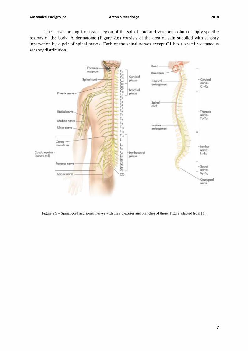
The nerves arising from each region of the spinal cord and vertebral column supply specific
regions of the body. A dermatome (Figure 2.6) consists of the area of skin supplied with sensory
innervation by a pair of spinal nerves. Each of the spinal nerves except C1 has a specific cutaneous
sensory distribution.
Figure 2.5 – Spinal cord and spinal nerves with their plexuses and branches of these. Figure adapted from [3].

Anatomical Background António Mendonça 2018
8
2.2 - Integration of Nervous System Functions [1]
The human nervous system produces responses with a degree of complexity that depends on the
interpretation of the stimuli received. The nervous system is indeed versatile as it can produce simple
responses such as reflexes or involve more complex mechanisms – the tracts (ascending and descending
pathways).
Although the spinal cord has a crucial role in the transmission and partly on the integration of
neural information, the interpretation and the processing of this kind of information occur mainly in the
encephalon. Besides that, the more complex responses triggered by the nervous system are usually
generated and/or developed by the encephalon.
The simplest kind of response that the nervous system can give is the reflex. A reflex is an
involuntary reaction in response to a stimulus applied to the periphery of the human body and transmitted
to the CNS. Reflexes allow a person to react to stimuli more quickly than is possible if conscious thought
is involved. A reflex arc is the neuronal pathway (basic functional unit) by which a reflex occurs (see
Figure 2.2). The reflex arc is, in other words, the basic functional unit of the nervous system because it
is the simplest pathway capable of receiving a stimulus and developing a proper response. A reflex arc
is usually composed by five segments (Figure 2.2): (1) a sensory receptor; (2) a sensory neuron; (3) in
some reflexes, interneurons, which are neurons that establish the communication between sensory
neurons and motor neurons; (4) a motor neuron; and (5) an effector organ (muscle or gland). The
simplest reflex arcs don’t involve interneurons. In fact, reflexes themselves vary in their complexity.
Some reflexes involve simple neural pathways and few or no interneurons while others have more
Figure 2.6 – Dermatome map. Figure adapted from [1].

Anatomical Background António Mendonça 2018
9
complex pathways and even integration centers. However, most reflexes occur in the spinal cord or in
the brainstem rather than in the higher brain centers.
One example of a reflex occurs when a person’s finger touches a very hot surface. In this order,
the heat stimulates pain receptors in the skin and consequently action potentials are produced. These
action potentials are conducted to the spinal cord via sensory neurons. In the spinal cord the sensory
neurons synapse with interneurons that, in turn, synapse with motor neurons that conduct action
potentials along their axons to flexor muscles in the upper limb that is receiving the stimulus. These
same muscles contract and pull the finger away from the hot surface. During the execution of this reflex
no conscious thought is required and the withdrawal of the finger from the painful stimulus begins before
the person is consciously aware of any pain.
2.2.1 - Sensory Functions [1]
The CNS constantly receives a variety of stimuli that have origin both inside and outside the
body. Sensory input to the brainstem and diencephalon helps maintain the homeostasis. Input to the
cerebrum and cerebellum keeps people informed about the surrounding environment and allows the
CNS to control motor functions. A small portion of the sensory input results in perception, the awareness
of the stimuli. Perception require the following steps:
1. Stimuli originated from the inside or outside of the body are detected by sensory receptors
and converted into action potentials that propagate to CNS through the nerves.
2. In the CNS, the nerve pathways carry the action potentials to the cerebral cortex and other
areas of CNS.
3. The action potentials that reach the cerebral cortex are translated, allowing the person to
be aware of the stimulus.
2.2.1.1 - Ascending Tracts [1]
The spinal cord and brainstem contain ascending tracts (pathways) that transmit information via
action potentials from the peripheral nervous system to various parts of the brain (Figure 2.7). Each tract
is involved with a limited type of sensory input, such as pain, temperature, touch, position or pressure,
because each tract contains axons from specific sensory receptors specialized to detect a specific type
of stimulus.
The names of the most part of ascending tracts in the CNS reflect their origin and termination.
To each path is usually given a compound name in which the first half of the word indicates its origin
and the second half of the word indicates its termination. The ascending tracts usually begin with the
prefix spino-, indicating its origin in the spinal cord. Exception to this rule of nomenclature is the dorsal
column tract.
Most ascending tracts consist of two or three neurons in sequence, from the periphery to the
brain. Almost all neurons that relay information to the cerebrum terminate in the thalamus. Another
neuron then conducts the information from the thalamus to the cerebral cortex. The spinothalamic tract
responsible for the transmission of action potentials dealing with pain and temperature to the thalamus
and on to the cerebral cortex, is an example of ascending tract. The already mentioned dorsal column
tract, which transmits action potentials dealing with touch, position and pressure, is another example
(Figure 2.8).
Typically, sensory tracts cross from one side of the body in the spinal cord or brainstem to the
other side of the body (Figure 2.8). Thus, the right side of the brain receives sensory inputs from the left
side of the body and vice versa.

Anatomical Background António Mendonça 2018
10
Ascending tracts can also terminate in the brainstem or cerebellum. For example, the anterior
and posterior spinocerebellar tracts transmit information about body position to the cerebellum.
2.2.1.2 – Sensory Areas of the Cerebral Cortex [1]
Figure 2.9 depicts a lateral view of the left cerebral cortex with some of the sensory and motor
areas indicated. Ascending tracts project to specific regions of the cerebral cortex, called primary
Figure 2.7 – Ascending tracts of the spinal cord. Figure adapted from [4].
Figure 2.8 – Dorsal Column / Medial Lemniscal Pathway. Figure adapted from [5].

Anatomical Background António Mendonça 2018
11
sensory areas, where sensations are perceived. The primary somatic sensory cortex (somatosensory
cortex), or general sensory area, is found in the parietal lobe posterior to the central sulcus.
Sensory fibers carrying general sensory input (related to pain, temperature, position…) synapse
in the thalamus. In turn, the thalamus projects neurons that relay information to the primary somatic
sensory cortex. Thus, sensory fibers from specific parts of the body project to specific regions of the
primary somatic sensory cortex. The primary somatic sensory cortex is organized topographically in
relation to the general plan of the body. As it can be seen in the Figure 2.9 the sensory impulses that
drive the stimuli from the lower limb and trunk project into the uppermost portions of the somatosensory
cortex.
The cortical areas immediately adjacent to the primary sensory areas (Figure 2.9), called
association areas, are deeply involved in the process of recognition.
2.2.2 - Motor Functions [1]
The motor system of the brain and spinal cord is responsible for maintaining the body’s posture
and balance, as well as moving the trunk, head, limbs, tongue, and eyes and communicating through
facial expressions and speech. The reflexes mediated through the spinal cord and brainstem are
responsible for some body movements that occur without a conscious thought (involuntary movements).
On the other hand, voluntary movements are consciously activated to achieve a specific goal, such as
walking. Although consciously activated, the components of most voluntary movements occur
automatically. For instance, once a person starts walking, she doesn’t have to think about the moment-
moment control of every muscle because there are neural circuits that control automatically the
movement of her limbs. After a person learns to execute complex tasks, like walking, these can be
performed in a relatively automatic way.
Figure 2.9 – Sensory and motor areas of the lateral side of the left cerebral cortex. Figure adapted from [6].

Anatomical Background António Mendonça 2018
12
Voluntary movements result from the stimulation of upper and lower motor neurons. Upper
motor neurons have their cell bodies in the cerebral cortex or in nuclei of the brainstem. Lower motor
neurons have their cell bodies in the anterior horn of the spinal cord gray matter or in cranial nerve
nuclei, in the brainstem. Axons of these neurons leave the central nervous system and extend through
spinal and cranial nerves to innervate skeletal muscles.
Voluntary movements depend on the following steps:
1. The initiation of most voluntary movements begins in the premotor area of the cerebral
cortex and leads to the stimulation of upper motor neurons.
2. The axons of upper motor neurons form descending pathways that synapse with lower motor
neurons. In turn, the axons of lower motor neurons stimulate the contraction of skeletal
muscles.
3. The cerebral cortex interacts with the basal nuclei and the cerebellum to plan and coordinate
the execution of movements.
2.2.2.1 – Motor Areas of the Cerebral Cortex [1]
The primary motor cortex is found in the posterior portion of the frontal lobe, directly anterior
to the central sulcus (Figure 2.9). Action potentials initiated in this region control voluntary movements
of skeletal muscles. Upper motor neuron axons project from specific regions of this cortex to specific
parts of the body so that a topographic map of the body exists in the primary motor cortex, with the head
inferior and lower limbs superior, analogous to the topographic map of the primary somatic sensory
cortex (Figure 2.9).
The premotor area of the frontal lobe is the portion of the cortex where motor functions are
organized before being initiated in the primary motor cortex. For instance, if a person decides to take a
step, the neurons of the premotor area are first stimulated, and the determination is made there as to
which muscles must contract, in what order, and to what degree. Action potentials are then passed to the
upper motor neurons of the primary motor cortex, which initiate each planned movement.
The motivation and foresight to plan and initiate movements occur in the anterior portion of the
frontal lobes, called the prefrontal area (Figure 2.9).
2.2.2.2 – Descending Tracts [1]
The names of the descending tracts are based on their origin and termination. For example, the
corticospinal tracts (Table 2.1) are so named because they begin in the cerebral cortex and terminate in
the spinal cord. The corticospinal tracts are considered direct because they extend directly from the
upper motor neurons in the cerebral cortex to the lower motor neurons in the spinal cord (a similar direct
tract extends to lower motor neurons in the brainstem). Other tracts are designated after the region of
the brainstem from which they originate. Although these tracts begin in the brainstem they are indirectly
commanded by the cerebral cortex, basal nuclei and cerebellum. These tracts are called indirect because
no direct connection exists between the cortical and spinal neurons.

Anatomical Background António Mendonça 2018
13
The descending tracts control different types of movement (Table 2.1). Tracts in the lateral
columns (Figure 2.10 and Figure 2.11) are most important in controlling goal-directed limb movements,
such as reaching and manipulating. The lateral corticospinal tract performs an especially important
function related to the speed and precision of skilled movements of the hands. Tracts in the ventral
columns, such as the reticulospinal tract, have the important role of maintaining posture, balance, and
limb position through the control of neck, trunk, and proximal limb muscles.
The lateral corticospinal tract is a good example of how descending pathways are organized. It
begins in the cerebral cortex and descends into the brainstem (Figure 2.11). At the inferior end of the
pyramids of the medulla oblongata the axons crossover to the opposite side of the body and continue
through the spinal cord. Crossover of axons in the brainstem or spinal cord to the opposite side of the
body is typical of descending pathways. Thus, the left side of the brain controls skeletal muscles on the
right side of the body, and vice versa. The upper motor neurons synapse with interneurons and these, in
turn, synapse with lower motor neurons in the brainstem or spinal cord. Lastly, axons of the lower motor
neurons extend to the skeletal muscle fibers.
Pathway Function
Direct
Lateral corticospinal Muscle tone and skilled movements, especially
of hands.
Anterior corticospinal Muscle tone and movement of trunk muscles.
Indirect
Rubrospinal Movement coordination.
Reticulospinal Posture adjustment, especially during
movement.
Vestibulospinal Posture and balance
Tectospinal Movement in response to visual reflexes.
Figure 2.10 – Descending tracts of the spinal cord. Figure adapted from [4].
Table 2.1 – Descending tracts (see figures 2.9 and 2.10). Table adapted from [1].

Anatomical Background António Mendonça 2018
14
2.3 – Spinal Cord Injury
Since the focus of this dissertation consists of the analysis of the gait in subjects with
neurological impairment, specifically spinal cord injuries, it is relevant to describe in this subchapter
some aspects related with this kind of injuries.
A spinal cord injury (SCI) occurs when the bony protection structure surrounding the cord is
damaged by way of fractures, dislocation, burst, compression, hyperextension or hyperflexion. In simple
words, a SCI (Figure 2.12) is a global definition for the damage of a spinal cord section that causes
changes in its function, either temporary or permanent. Spinal cord injuries can interrupt ascending
and/or descending tracts. Reflexes can still function below the level of the injury, but sensations and/or
motor functions and reflex modulation may be disrupted. Therefore, it is easy to understand that a SCI
can affect severely the performance of daily normal activities, such as walking. Actually, the walking
capability of a person after the occurrence of a SCI will strongly depend on the severity (complete or
incomplete) and the injury site (which section of the vertebral column was damaged) [1,9].
According to J.E. Lasfargues et al. [8], just in United States, the annual number of traumatic
spinal cord injury cases admitted to hospitals was projected to increase from approximately 11 500 in
Figure 2.11 – Direct pathways. Upper motor neuron axons descend to the medulla oblongata. Most axons decussate in
the medulla oblongata and descend in the lateral corticospinal tracts in the spinal cord. Some axons continue as the
anterior corticospinal tracts and decussate in the spinal cord. Figure adapted from [4].

Anatomical Background António Mendonça 2018
15
1994 to almost 13 400 in 2010. Age adjusted post-hospitalization incidence rate in 1994, in United
States, was estimated at approximately 38 per million [8]. Still considering the same article [8], in 2010,
there were approximately 247 000 Americans victims of a SCI living in United States. On the other
hand, according to A. Singh et al. [42], there are in the central region of Portugal, each year, 58 new
cases of SCI considering one million of Portuguese individuals. According to S. Ferro et al. [43], a study
conducted at acute-care SCI hospitals and SCI institutes from 11 Italian regions, realized between the
1st of October of 2013 and the 30th of September of 2014, estimated that the crude incidence rate of
traumatic SCI was 14.7 cases per million per year.
The most common cause of spinal cord dysfunction is trauma caused by motor vehicle
accidents, falls, shallow diving, acts of violence, and sports injuries. Damage can also occur from various
diseases acquired at birth or later in life, from tumors, electric shock, and loss of oxygen related to
surgical or underwater mishaps. Most spinal cord injuries that occur can be classified as acute contusions
of the cervical portion of the cord and do not completely sever the spinal cord (incomplete injuries) [1].
A SCI is classified as complete or incomplete. An incomplete injury means that the ability of
the spinal cord to convey messages to or from the brain is not completely lost. Additionally, this means
that, some sensation (even if it’s faint) and movement is possible below the level of injury. A complete
injury is characterized by a total lack of sensory and motor function below the level of injury. The
absence of motor and sensory function below the level of injury does not necessarily mean that don’t
exist remaining intact axons or nerves crossing the injury site, just that they are not functioning
conveniently due to the lesion [9].
At the time of SCI, two types of tissue damage occur: (1) primary mechanical damage and (2)
secondary tissue damage extending into a much larger region of the cord than the primary damage. The
only treatment for the primary damage is prevention itself, such as wearing seatbelts when driving
(mainly in automobiles) and not diving into shallow water. Once the accident occurs, there is practically
nothing that can be done to repair the primary damage. Secondary spinal cord damage, which begins
within minutes of the primary damage, is caused by ischemia (lack of blood supply), edema (fluid
accumulation), ion imbalances, the release of “excitotoxins” (such as glutamate), and inflammatory cell
invasion. Unlike primary damage, much of the secondary damage can be prevented or reversed if the
treatment is prompt. Giving the patient large doses of methylprednisolone, a synthetic anti-inflammatory
steroid, within 8 hours of the injury can dramatically reduce the effects of the secondary damage to the
cord. Other alternatives for the treatment of the secondary spinal cord damage include the anatomical
realignment and stabilization of the vertebral column and still the decompression of the spinal cord. All
the rehabilitation procedures applied in medicine intend to retrain patients to use whatever residual
connections that still exist across the site of damage [1].
Although the spinal cord was formerly considered incapable of regeneration following severe
damage, researchers have learned that most of the neurons of the adult spinal cord survive an injury and
begin to regenerate, growing about 1 mm into the site of damage, before regressing to an inactive,
atrophic state. The major block to adult spinal cord regeneration is the formation of a scar, consisting
mainly of astrocytes, at the site of injury. Myelin in the scar apparently inhibits regeneration. However,
and despite the arduous work, researchers are still trying to optimize mechanical tools and chemical
factors that might “stimulate” the regeneration of the spinal cord following an injury [1].
Doctors usually assess their patients for spinal cord injuries based on two factors: the location
and type of injury a patient has sustained, and the consequent symptoms. Anyone who has fallen,
suffered a blow, or lost consciousness may have suffered a SCI. If a person also experiences headaches,
loss of movement, tingling, difficulty moving, or difficulty breathing, the conjugation of all these
symptoms may be an indicative of the occurrence of a SCI. Yet, no single tests can assess directly all
spinal cord injuries. Instead, doctors rely on a variety of protocols that include a clinical evaluation of

Anatomical Background António Mendonça 2018
16
symptoms presented by a patient and imaging tests. A doctor can order MRI imaging or other forms of
radiological imaging to view a person’s spinal column, spinal cord or brain [46].
2.3.1 – Implications of a Spinal Cord Injury [9]
Since the spinal cord coordinates body movement and sensation, an injured spinal cord loses
some or all abilities (depending if the injury is incomplete or complete) to send and receive messages
responsible for controlling sensory, motor, and autonomic function.
The location of the spinal cord injury dictates the parts of the body that are affected. After a
complete neurological examination, the doctor responsible will assign a level of injury and determine if
the injury is complete or incomplete. The initial level of injury and function may change upon
rehabilitation.
The guidelines that follow are general guidelines and it is important to remember that individual
outcomes will vary for each patient.
Cervical Spinal Cord Injury C1-C8
Cervical level injuries cause tetraplegia or weakness in both superior and inferior limbs. This
area of the spinal cord controls signals to the back of the head, neck, arms, hands and diaphragm.
Since the neck region is very flexible it is difficult to stabilize cervical spinal cord injuries.
Patients may be placed in a brace or stabilizing device.
All regions of the body below the level of injury or top of the back may be affected. Often, a
cervical injury is accompanied by the loss of physical sensation, respiratory issues, inability to regulate
body temperature, as well as bowel, bladder and sexual dysfunction.
Thoracic Spinal Cord Injury T1-T12
Thoracic level injuries are less common due to the protection given by the rib cage.
Thoracic injuries can cause paralysis (paraplegia) or weakness of the inferior limbs along with
loss of physical sensation, bowel, bladder, and sexual dysfunction.
Figure 2.12 – Illustration of a spinal cord injury. Figure adapted from [15].

Anatomical Background António Mendonça 2018
17
In most cases, upper limbs’ function is unaffected. This area of the spinal cord controls signals
to some of the muscles of the back and part of the abdomen.
With these types of injuries most patients initially wear a brace on the trunk to provide extra
stability and help build up core muscles.
Lumbar Spinal Cord Injury L1-L5
Lumbar level injuries result in paralysis (paraplegia) or weakness of the inferior limbs. Loss of
physical sensation, bowel, bladder and sexual dysfunction can occur. However, superior limbs’ function
is usually unaffected.
The lumbar area of the spinal cord controls signals to the lower parts of the abdomen and the
back, the buttocks, some parts of the external genital organs, and parts of the inferior limbs. These
injuries often require surgery and external stabilization.
Sacral Spinal Cord Injury S1-S5
Sacral level injuries primary cause loss of bowel and bladder function as well as sexual
dysfunction. These injuries can cause weakness or paralysis of the hip and lower limbs.
The sacral area of the spinal cord controls signals to the thighs and lower parts of the inferior
limbs, the feet and sexual organs.
2.3.2 – Incomplete Spinal Cord Injuries [46]
Incomplete spinal cord injuries are increasingly common, thanks in part to a better treatment
and an increased knowledge about how to respond (and how not to respond) to a suspected SCI. This
kind of injury now accounts for more than 60 % of spinal cord injuries.
Some of the most common types of incomplete or partial spinal cord injuries include: the
anterior cord syndrome, the central cord syndrome and the Brown-Sequard syndrome.
The anterior cord syndrome is an injury, to the front of the spinal cord, that damages the motor
and sensory pathways (ascending and descending tracts) in the spinal cord. A person with this kind of
injury usually may retain some sensation but struggles with movement.
The central cord syndrome is an injury to the center of the cord, and damages nerves that carry
signals from the brain to the spinal cord. Loss of fine motor skills, paralysis of the superior limbs, and
partial impairment (usually less pronounced) in the inferior limbs are common. Some survivors also
suffer a loss of bowel or bladder control or lose the ability to sexually function.
The Brown-Sequard syndrome is the product of damage to one side of the spinal cord. The
injury may be more pronounced on one side of the body, i.e. movement may be impossible on the right
side, but may be fully retained on the left side. The degree to which Brown-Sequard patients are injured
greatly varies from patient to patient.
2.3.3 – ASIA Impairment Scale
The extent and severity of a patient’s spinal cord injury are described by a system of tests defined
as the American Spinal Injury Association (ASIA) Impairment Scale [47,48]. This set of tests is most
commonly known as AIS (American Impairment Scale). This scale helps to determine future
rehabilitation and recovery needs. It is ideally completed within 72 hours after the initial injury. The
scale’s grade is based on how much sensation a person can feel at multiple points on the body, as well

Anatomical Background António Mendonça 2018
18
as on motor function tests. This scale uses the following grades to evaluate the extent and severity of a
patient’s spinal cord injury:
A = Complete: complete lack of motor and sensory function below the level of injury (including
anal area).
B = Incomplete: some sensation below the neurologic level of injury (including anal sensation).
C = Incomplete: some muscle movement (motor function) is preserved below the neurologic
level of injury, but more than half of key muscles below the level of injury cannot move against gravity.
D = Incomplete: motor function is preserved below the neurologic level of injury, and most key
muscles below the level of injury are strong enough to move against gravity.
E = Normal: sensory and motor functions are normal.
As can be concluded, considering the occurrence of a spinal cord injury, the grade A
corresponds to the most severe degree that AIS can present, while the grade D corresponds to the least
severe degree.

Robotic Neurorehabilitation António Mendonça 2018
19
CHAPTER 3 – ROBOTIC NEUROREHABILITATION
The occurrence of a spinal cord injury can incapacitate a person to perform daily tasks such as
walking. As known, walking is an important part of being independent and overcoming daily obstacles.
If a person has lost the ability to walk normally due to a trauma, for example, then in most cases
(especially for patients with incomplete motor injuries), physical therapy will help to recover motor
functions given as lost. The purpose of neurorehabilitation consists basically of the execution of specific
exercises that promote motor plasticity (achieved by the neuromuscular recruitment dependent on the
activation of specific neural pathways [10]). The final purpose consists in restoring and accelerating
motor activity and minimizing functional deficits [11].
The neurorehabilitation process is governed by three fundamental principles of motor learning
[10]:
1st Principle – Practice: The recurrent practice of motor exercises generates motor learning;
2nd Principle – Specificity: The best way to improve the performance of a motor task is to
perform this specific motor task repetitively;
3rd Principle – Effort: Patients need to maintain a high degree of involvement to facilitate
and accelerate motor learning.
Regarding the rehabilitation of gait, the conventional physiotherapy, besides costly, in terms of
money and time, often requires an exhaustive physical effort on the part of the physiotherapists in charge
of performing it. Robotic assisted rehabilitation (RAR) tools have emerged with the objective of
reducing the cost, in terms of time, and attenuating the hard-physical effort demanded to physiotherapists
(not replacing them at all but assisting them in fulfilling their function). Additionally, with the purpose
of enhancing and accelerating conventional rehabilitation, RAR devices are well suited to produce
specific, intensive, task-oriented motor training for moving the patient’s lower limbs under the
supervision/help of a therapist [34]. The use of such tools also makes possible the evaluation of the level
of motor recovery since it is possible to quantitatively measure force and movement patterns [12].
Besides that, some RAR tools also have the advantage of being able to provide accurate sensorimotor
feedback, a feature that is not possible to acquire from conventional gait physiotherapy [56]. However,
this kind of systems shall follow the assist-as-needed approach. This approach states that RAR tools
shall have a controller developed purposely to help an individual only when is necessary, stimulating
and encouraging the user to put an effort on the specific task to be performed [12,20].
Many RAR tools used in the motor rehabilitation of the lower limbs have as an integral part of
their constitution a specific model of an exoskeleton.
An exoskeleton is an electromechanical device that is worn by a human operator and is intended
to enhance the user’s physical performance. From the medical point of view, exoskeletons may play a
prominent role in locomotor therapy of post-stroke patients or people with a spinal cord injury, since
these electromechanical systems may constitute an additional tool capable of re-educating the
compromised gait that these patients might present. Following this idea, exoskeletons may be a viable
alternative to the wheelchair, often necessarily used by these patients, providing mobility and enabling
these people to perform, as much as possible, normal daily activities such as climbing stairs.
Exoskeletons may still be a study tool for the medical community since they may contribute to a richer
understanding of the posture and movement of the human body [13].
An exoskeleton has as main constituents:
The mechanical structure;

Robotic Neurorehabilitation António Mendonça 2018
20
The power system that includes actuators and power supplies or batteries;
The control system with sensors.
Following the execution of a movement by the user, most exoskeletons usually follow a
procedure (algorithm) that is segmented into four steps [13]:
1) Analysis of the current situation: posture, limb position, etc., based on sensory information
acquired from angular sensors, pressure sensors, gyroscopes, accelerometers, etc., that are
incorporated in the mechanical structure of the exoskeleton. On the other hand, the analysis
of the current situation may also be achieved based on signals collected by
electromyography (EMG) or other bioelectrical activity (for example muscle contraction)
sensors, which are attached to the user’s skin surface.
2) When the user intends to move: the exoskeleton control system analyses the signals from
the sensors and determines which movement the user intends to perform.
3) The control system selects a preprogramed movement pattern, adjusts it to the user’s current
position and finally supports the movement by using actuators (electromechanical muscles)
that employ the appropriate level of force/help.
4) After completing the movement, the control system analyses the new situation – posture,
position of the limbs, etc. – evaluating and preparing the next possible user movements.
Almost all functional exoskeletons rely on additional support aids to ensure balance. On one hand,
healthy users will perform proper foot placement and other actions to ensure balance stability. On the
other hand, is highly probable that impaired people will need additional devices such as crutches [34].
In the case of treadmill-based exoskeletons the balance control is usually achieved by means of a simple
body weight support system with an adjustable vertical force [12].
Due to the close interaction between the user and exoskeleton, these robotic devices must be, as
close as possible, mechanically compatible with the human anatomy. In this sense, all exoskeletons must
move in line with the user without compromising (resisting or obstructing) the safe performance of
movements that are executed [14].Concerning the design of an exoskeleton, especially in the
construction of the joints that constitute the exoskeleton, there are certain fundamental biomechanical
factors that must be considered, such as degrees-of-freedom (DOF), range-of-motion (ROM), joint
torques requirements, joint rotational velocity, and joint angular bandwidth [14]. Other factors, such as
the type of actuation (which can be active, quasi-active or passive – this choice will have a preponderant
impact on the amount of energy needed to feed the mechanical system), the degree of anthropomorphism
(a device is seen as anthropomorphic when the elements constituting the exoskeleton frame correspond
in terms of size and of kinematic alignment to the part/limb of the human body that is being assisted),
the weight distribution/inertia of the exoskeleton and the physical interface are also relevant in the
construction of a exoskeleton’s design [14].
RAR devices can be classified according to the motion they apply to the user’s body. On one
hand, exoskeletons have axes aligned with the anatomical planes of the wearer. In gait rehabilitation,
exoskeletons provide direct control over individual joints, such as the hip, the knee and/or the ankle,
which can minimize abnormal posture or movement [34,56]. On the other hand, end-effector operative
machines work by applying mechanical forces to the distal segments of inferior limbs. In end-effector
devices, subjects’ feet are normally strapped over footplates, whose trajectories simulate specific stages
of the human gait [56,57]. Another possible classification, is between devices in which the user is moved
in a fixed place and those that move the user around the environment. Therefore, RAR devices can also
be classified as static or dynamic [34].

Robotic Neurorehabilitation António Mendonça 2018
21
Both end-effector operative machines and exoskeleton robotic devices have their own strengths
and weaknesses. Therefore, it is important to consider the rationale of the two types of devices and the
related benefits and disadvantages of each one. On one hand, end-effector walking devices offer the
advantage of easy setup, allowing the user to extend his/her knee with more freedom. However, end-
effector devices suffer from limited control of the proximal joints of inferior limbs, which could result
in abnormal movement patterns. In addition, the task of maintaining balance may be more demanding
(since the required degree of balance depends on how the harness is setup and whether the user holds
the hand rails). In case of exoskeletons, a clear advantage is that gait cycles can be controlled more
easily. On the other hand, the construction of exoskeleton-type devices is more complex and more
expensive when compared with the end-effector type, since exoskeleton-type devices are outfitted with
programmable drives or passive elements responsible for moving the knees and hips during the phases
of gait [34,55,56, 57].
3.1 – Biomechanics of Walking
Locomotion is the ability to move from one place to another. In humans, walking is the main
method of locomotion. Walking involves all joints of the lower limb and is described by an “inverted
pendulum” motion, in which the body vaults over the non-moving limb [40].
The intensive study of the human walking biomechanics, accomplished by the scientific
community, is really challenging, since it requires a lot of time and patience, but it is crucial for the
design of new RAR tools. Therefore, before reviewing any RAR tool considered in the context of this
dissertation, as well the status of gait analysis using RAR tools, it is pertinent to address some
biomechanical aspects related to human walking.
In biomechanical terms the human inferior limb can be considered as a seven DOF structure,
with three rotational DOF at the hip (spherical joint), one at the knee (condylar joint), and three at the
ankle/foot joint complex [16]. Figure 3.1 presents a description of the human anatomical planes. The
hip joint allows the flexion/extension movement in the sagittal plane, the abduction/adduction
movement in the coronal plane and internal/external rotations in the transverse plane. The knee joint
actually has two DOF, however only one is generally considered, because the internal/external rotations
of the knee in the transverse plane constitute very limited movements. Thus, the knee joint is usually
related only to the flexion/extension movement in the sagittal plane. The ankle/foot joint complex results
from the combination of the ankle joint and the transverse tarsal joint. In turn, the transverse tarsal joint
is not a single joint but rather the combination of the talo-navicular and the calcaneo-cuboid joint [19].
The ankle/foot joint complex allows the flexion/extension movement in the sagittal plane, as well as the
eversion/inversion movement in the coronal plane and internal/external rotations in the transverse plane
[14,16].
Figure 3.2 shows a simplified diagram of the processes involved in human walking. A gait cycle,
segmented according to Figure 3.2, corresponds to the period that separates the occurrence of two
identical events during gait. Any event can be selected for the beginning of the gait cycle since the
various events follow each other continuously. However, the human gait cycle is typically represented
as starting (0%) and ending (100%) at the point of heel strike on the same foot, with heel strike on the
adjacent foot occurring at, approximately, 60 % of gait cycle [16]. Each gait cycle is divided into two
phases: stance and swing. The stance phase corresponds to the portion of gait cycle in which the foot,
whose heel strike was considered the initial event, (in Figure 3.2, corresponding to the right foot) is in
contact with the ground, constituting 60% of the gait cycle. The swing phase corresponds to the period
in which the same foot is in the air, constituting the remaining 40% of the gait cycle [16]. The swing
phase begins when the toes of the foot, whose heel strike was considered the initial event, leave the
ground (designated as the toe off moment – in Figure 3.2 designated as foot off).

Robotic Neurorehabilitation António Mendonça 2018
22
3.1.1 – Stance Phase [19]
A more convenient and precise way to describe the stance phase of gait is to consider the three
sub-stages that a single foot undergoes (considering the right leg in Figure 3.1). They are as follows: 1st
Double Support Phase, Single Support Phase and 2nd Double Support Phase.
3.1.1.1 – 1st Double Support Phase
Figure 3.2 – Representation of a segmented human gait cycle. Figure adapted from [17].
Figure 3.1 – Description of the human anatomical planes. Figure adapted from [18].
Robotic Neurorehabilitation António Mendonça 2018
23
The 1st Double Support Phase starts on the moment that the heel first touches the ground and
lasts until the whole foot is on the ground (Figure 3.1).
3.1.1.2 – Single Support Phase
The beginning of the Single Support Phase is defined as the moment the whole foot is on the
ground. At the end of the middle Single Support Phase (Figure 3.1) the body’s center of gravity already
passed over top of the foot. The body’s center of gravity is located approximately in the pelvic area in
front of the lower spine when we are standing and walking. The purpose of the initial and middle Single
Support Phase is to allow the foot to serve as a shock absorber, helping to cushion the force of body
weight landing on the foot. Once the body’s center of gravity has passed in front of the neutral position,
a person is said to be in the terminal Single Support Phase. This last stage of the Single Support Phase
ends when the heel lifts off the ground (Figure 3.1). During this stage, the foot needs to go from being
a flexible shock absorber to be a rigid lever that can serve to propel the body forward.
3.1.1.3 – 2nd Double Support Phase
The 2nd Double Support Phase begins when the heel begins to lift off the ground. During this
phase, the foot functions as a rigid lever to move the body forward. During this stage, the forces that go
through the foot are quite significant: often two to three times a person’s body weight. This happens
because the foot creates a lever arm (centered on the ankle), which serves to magnify body weight forces.
The 2nd Double Support Phase ends with the toe off (in the Figure 3.1 referred as foot off), a conventional
designation that characterizes the moment when the toes of the considered foot (the right in this case)
leave the ground. The toe off moment also represents the end of the stance phase and the beginning of
the swing phase.
3.1.2 – Swing Phase [40]
The swing phase accounts for 40 % of the gait cycle. It can be divided into the leg lift and swing
phases.
3.1.3 – Paraparetic Gait [58]
A spinal cord injury can cause a paraparetic gait. Paraparetic gait usually results from the
damage of the descending corticospinal tract which may be characterized in an early stage by a
generalized stiffening of the lower limbs. In fact, the patient may find impossible to walk quickly or run.
Paraparetic gait is recognized by a stiff, scissor-like walking with leg adduction and extension. In short,
this condition is associated with weakness and hyperreflexia in both lower limbs.
3.1.4 – High-Steppage Gait [19]
Another example of an abnormal gait is a high-steppage gait pattern. This kind of gait pattern
is often seen in patients whose muscles from the anterior compartment of the leg do not function
normally (considering, for example, patients that present a droop foot). This impairment of the anterior
compartment muscles causes the foot to slap onto the ground during the 1st Double Support Phase of
walking. Patients normally try to overcome this problem by bending their knee more than normal during
the swing phase of gait to lift the foot higher off the ground.
Robotic Neurorehabilitation António Mendonça 2018
24
3.2 – Robotic Assisted Rehabilitation Tools
Throughout the 21st century, several RAR tools have been specifically designed to help
reestablish the motor mobility of people severely affected by neurological diseases, that present
problems to walk normally.
The subsections that follow describe the two RAR tools used in the context of this dissertation:
the Lokomat exoskeleton Pro version 6.0 and Gait Trainer GT1. These two RAR tools, described with
detail in the following subsections, were used in the acquisition of EMG data recorded from a series of
experiments. These experiments were carried out at FSL and involved several subjects, 10 healthy
subjects, 5 subjects with complete spinal cord injury and 5 subjects with incomplete spinal cord injury.
3.2.1 – Lokomat [22,23,34]
The Lokomat exoskeleton Pro version 6.0 (Hocoma AG, Volketswil, Switzerland) (Figure 3.3)
is comprised of two actuated orthoses that are attached to the user’s inferior limbs by means of cuffs
and straps. This bilaterally driven exoskeleton is usually used with a body weight support (BWS) system
and a treadmill. The geometry (hip width and length of the lower limbs) of the orthoses, and the size
and position of leg cuffs must be adjusted to the subject’s individual anthropometry, ensuring that
walking in the device is as natural and comfortable as possible.
The hip and knee joints of Lokomat are actuated by linear actuators, in the sagittal plane, and
as such guide the user’s inferior limbs to move along a preprogrammed kinematic gait pattern. This
predefined pattern is based on joint movements derived from trajectories of healthy subjects but can be
fine-tuned by adjusting the hip and knee angles to meet walkers’ functionality. Ankle movements are
not actuated directly by the orthoses, but can be stabilized by elastic foot lifters, to prevent foot drop
and concomitant stumbling during the swing phase.
The ‘guidance’ provided by the Lokomat exoskeleton is realized by means of an impedance
controller, which allows the level of guidance to be set by a therapist. The level of guidance that is
offered determines how much lower limbs’ movements are permitted to deviate from a predefined
pattern. As long as the participant moves along the predefined trajectory, the controller does not act, but
once the limits are exceeded, joint torques are applied in order to move the lower limb back towards the
desired track. When the guidance level is set to its maximum (i.e. 100%), the subject is forced to strictly
follow the predefined trajectory without permitting any kind of deviance. On the other hand, when the
guidance level is set to nil (i.e. 0% - ‘free run’ mode), free movements of the inferior limbs are allowed
as torques are applied only to compensate interaction forces between the exoskeleton and the user that
result from inertia of the exoskeleton, gravity and friction.
In the present study, the level of guidance during the ‘Lokomat guided walking’ condition was
first set to 50%, which allows small deviations and requires a more active involvement of the walker
when compared to fully guided walking (the guidance level set to 100 %). At a later stage of the
experiments the guidance level of the exoskeleton was modified to 100%.

Robotic Neurorehabilitation António Mendonça 2018
25
3.2.2 – Gait Trainer GT1 [24,25,34]
Gait Trainer GT1 (Reha-Stim, Berlin, Germany) (Figure 3.4) is an end-effector type RAR
device which uses two footplates to generate a gait-like movement (simulating stance and swing phases
with an actual lifting of the foot during the swing). These footplates are designed and programmed to
provide a ratio of 60 percent to 40 percent between the stance and swing phases. It is important to refer
that user’s feet don´t enter in contact with the ground at any moment (the feet are always strapped to the
platforms).
According to S. Hesse et al. [24], the Gait Trainer GT1’s design is based on a double crank and
rocker gear system. It consists of two footplates positioned on two bars (couplers), two rockers, and two
cranks that provide propulsion (Figure 3.5). The low backward movement of the footplates simulates
the stance phase while the forward movement simulates the swing phase. This system generates a
different movement of the tip and the rear of the footplate during the swing stage. Basically, the tip of
the footplate follows an arc-like movement corresponding to the length of the rocker, while the rear end
is lifted, so that the footplate itself is inclined during swing. Furthermore, the crank propulsion is
modified by a planetary gear system to provide the ratio of 60 percent to 40 percent between stance and
swing phases. It consists of fixed sun gears and circulating planet gears of the same diameter. The foot
bars are eccentrically connected to the planet gears so that the rear end of the foot bars follows an
ellipsoid-like movement. The upper half of the revolution (corresponding to the swing) lasts 40 percent,
while the lower half of the revolution (corresponding to the stance) lasts 60 percent of one revolution
time. According to the user’s anthropomorphic features and walking capabilities, different gear sizes
and eccentricities can be mounted to vary the stride length and the phase duration.
In Gait Trainer GT1 there is no way to control the level of physical assistance (guidance level)
provided to individuals. Indeed, the system is very basic and only permits the physiotherapist to set the
Figure 3.3 – Lokomat Pro version 6.0 (picture courtesy of Hocoma). This picture shows a person strapped in a Lokomat
Pro version 6.0. The person is suspended in a harness from a wire above for body weight support and moved by
attachments at the lower back to the robotic exoskeleton. The subject’s legs are strapped in the exoskeleton which is
actuated at the hip and knee. The forefoot is stepped upwards with a spring to induce dorsiflexion. Figure adapted from
[12].
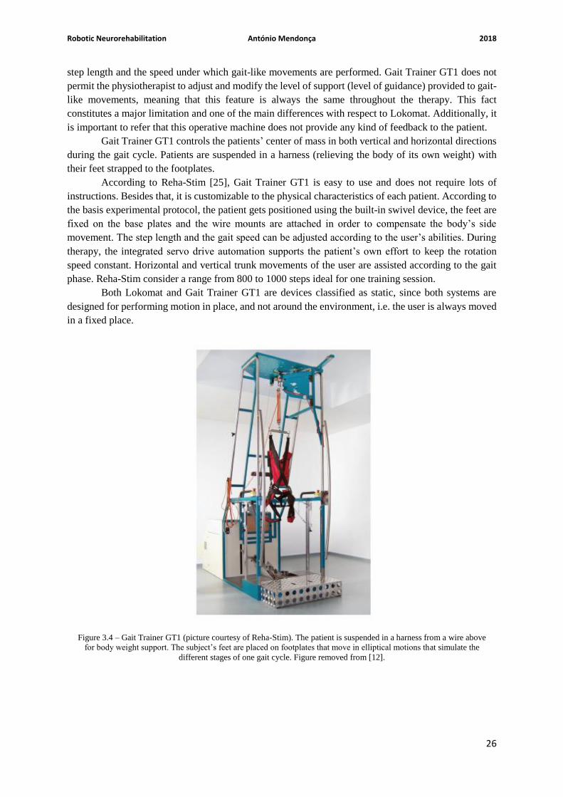
Robotic Neurorehabilitation António Mendonça 2018
26
step length and the speed under which gait-like movements are performed. Gait Trainer GT1 does not
permit the physiotherapist to adjust and modify the level of support (level of guidance) provided to gait-
like movements, meaning that this feature is always the same throughout the therapy. This fact
constitutes a major limitation and one of the main differences with respect to Lokomat. Additionally, it
is important to refer that this operative machine does not provide any kind of feedback to the patient.
Gait Trainer GT1 controls the patients’ center of mass in both vertical and horizontal directions
during the gait cycle. Patients are suspended in a harness (relieving the body of its own weight) with
their feet strapped to the footplates.
According to Reha-Stim [25], Gait Trainer GT1 is easy to use and does not require lots of
instructions. Besides that, it is customizable to the physical characteristics of each patient. According to
the basis experimental protocol, the patient gets positioned using the built-in swivel device, the feet are
fixed on the base plates and the wire mounts are attached in order to compensate the body’s side
movement. The step length and the gait speed can be adjusted according to the user’s abilities. During
therapy, the integrated servo drive automation supports the patient’s own effort to keep the rotation
speed constant. Horizontal and vertical trunk movements of the user are assisted according to the gait
phase. Reha-Stim consider a range from 800 to 1000 steps ideal for one training session.
Both Lokomat and Gait Trainer GT1 are devices classified as static, since both systems are
designed for performing motion in place, and not around the environment, i.e. the user is always moved
in a fixed place.
Figure 3.4 – Gait Trainer GT1 (picture courtesy of Reha-Stim). The patient is suspended in a harness from a wire above
for body weight support. The subject’s feet are placed on footplates that move in elliptical motions that simulate the
different stages of one gait cycle. Figure removed from [12].

Robotic Neurorehabilitation António Mendonça 2018
27
3.3 – RAR Tools: Status of Gait Analysis
This section presents, in general, the status of EMG analysis in patients with a spinal cord injury
involving the use of RAR tools, and a small description of what is being done with the two robotic
systems introduced in the previous subchapters.
Evidence of RAR tools efficacy in improving functional gait of stroke patients is becoming
stronger but several parameters of optimization, combinations with other techniques and the difference
in effect between subgroups are still not well understood. For stroke patients it has been shown that the
use of RAR devices together with conventional physiotherapy increases the odds of becoming gait
independent [26]. For patients with a spinal cord injury, evidence of locomotor training efficacy using
RAR tools is less clear as there is a lack of randomized controlled trials which makes the evaluation of
different approaches to locomotor training difficult [27]. In fact, there are still no standardized protocols
and specific medical guidelines for using this kind of robotic systems. Thus, to determine the correct
criteria for the use of robotic systems, it is necessary to prepare and conduct clinical trials involving a
large (statistically speaking) sample of individuals [13].
To improve the human understanding of the effect of locomotor training, using RAR tools, on
test subjects, the scientific community applies a widely and useful tool: gait analysis [28,54]. Measuring
and tracking the performance of patients, using RAR tools, is important to evaluate the functional
improvements that result from the use of such devices. During rehabilitation therapies, measurements
of the electrical activity of some specific muscles become relevant to analyze gait and, in turn, to
evaluate the effects of such training. If this kind of training works, the EMG curves generated by patients
should become more similar to the ones presented by healthy subjects.
However, there are some difficulties when working together with EMG and people with motor
disabilities. After the acquisition of EMG data, analyzing the patterns of activity into meaningful results
is difficult and most methods used in the analysis involve complicated statistical or mathematical
processes that might be hard for clinicians and others that are not very well versed in mathematics to
Figure 3.5 – Modified crank and rocker gear system including a planetary gear system to simulate stance and swing
phases with a ratio of 60 percent to 40 percent. Figure adapted from [24].

Robotic Neurorehabilitation António Mendonça 2018
28
understand. This has led to the use of many EMG parameters that ignore time and look at a grand average
of gait cycles or at sub-periods or points where the meaning of the whole pattern is lost [29,30].
There is already research on EMG curves obtained during locomotor training using robotic
devices [22,23,31]. Some of these studies attempt to assess differences between RAR devices in a
quantitative way [22,23,31]. For example, the article [22] analyzes the differences in muscle activity
and temporal step parameters between Lokomat guided walking and treadmill walking in post-stroke
hemiparetic patients and healthy subjects. This study has concluded that compared to treadmill walking,
Lokomat guided walking was associated with reductions in the amplitude of muscle activity in both
healthy subjects and stroke patients, and a reduction in temporal step asymmetry in stroke patients. The
article [22] also concluded that in patients, the reductions in muscle output were apparent irrespective
of whether muscle activity was abnormally high or abnormally low during the treadmill walking. The
article [23] studies the combined effects of body weight support (BWS) and gait speed on gait related
muscle activity, comparing the regular treadmill walking with the Lokomat guided walking. According
to K. van Kammen et al. [23], the results obtained have shown that the Lokomat exoskeleton alters the
temporal regulation of steps as well as the neuromuscular control of walking, and that the nature and
magnitude of these effects depend on complex interactions with gait speed and BWS. The article [23]
also claims, based on the results obtained, if normative gait patterns are desired, very low speeds and
high levels of BWS should be avoided when possible. The article [31] studies the alterations in muscle
activation patterns during robot-assisted walking (again, it is basically a comparison between walking
in a regular treadmill and walking in a Lokomat exoskeleton). Regarding Gait Trainer GT1, there are
some studies that evaluate the efficacy of this RAR tool [32,33,55,56,57], but not many that study EMG
curves during a locomotor training. Most of studies involving a gait trainer, of which the articles [32]
and [33] are part of, do not make use of EMG curves to evaluate the related gait. Instead, these studies
usually use other criteria such as the functional ambulation category (FAC), the RMA score (gross
functions of leg and trunk section), the modified Ashworth score testing for the ankle dorsiflexion of the
affected side and the mean gait velocity to evaluate and infer about the effects that this kind of device
has on patients.
The application of mathematical and statistical tools may prove to be useful to understand the
whole EMG curve both in research as well as in a clinical setting, in order to optimize the neuro-
rehabilitation process. The Linear Fit Method (LFM), that has been developed and validated for
kinematic data [21], is the linear regression of two data sets plotted against each other to obtain 3
parameters that describe offset, amplitude difference and shape similarity, as described by M. Iosa et al.
[21]. The LFM has shown a good reliability in comparing kinematic data from 34 patients with
cerebrovascular accident with 15 healthy subjects [21].
This dissertation aims at using the LFM, in conjugation with other mathematical operations, to
study the EMG activity recorded during the use of different robotic devices and during the over-ground
walking, to gain knowledge of how these devices influence muscle activity both in patients and healthy
subjects.
3.4 – EMG Signal
Electromyography is the study of electrical signals generated by the muscles. These signals are
rich in information about the functionality from the muscle and can be exploited for research purposes.
So, it is relevant to understand how they are generated in the human body.
3.4.1 – Muscle Physiology [1,7]

Robotic Neurorehabilitation António Mendonça 2018
29
Action potentials are the electrical signals that originate the muscle contraction. The action
potential is generated due to the capability of nerve cell membranes to allow the passage of Na+ ions
and K+ ions. These signals are propagated from the brain or spinal cord along axons of nerve cells to
skeletal muscle fibers and causes them to contract.
Plasma membranes are polarized, meaning that there is a voltage difference across each plasma
membrane. The voltage difference of an unstimulated cell is designated the resting membrane potential,
which is by norm about -85 mV. However, stimulation of a cell can cause depolarization of its plasma
membrane. If the depolarization makes the membrane potential reach a value called “threshold”, an
action potential is triggered. An action potential, typically takes about one to a few milliseconds to occur
and it is constituted by two stages: depolarization and repolarization. During the depolarization phase,
the interior of the cell becomes positively charged after cell stimulation because of the opening of Na+
channels present in the membrane. These positively charged ions make the interior of the cell less
negative and, if the threshold value is reached, more voltage-gated Na+ channels will open rapidly,
making the interior of the membrane positive for a brief time (about +20 mV – see Figure 3.6). This
voltage change provokes additional permeability changes in the plasma membrane, which makes
depolarization stop and repolarization start. During this stage, the Na+ channels close and the movement
of K+ toward the exterior of the cell increases, making the interior of the plasma membrane more
negative and the exterior more positive. After the resting membrane potential is reestablished, voltage-
gated K+ channels close and the action potential ends. The generation of an action potential, therefore
depends if the stimulus is strong enough to reach the threshold value and cause depolarization. This is
denominated as the all-or-nothing principle.
Although an action potential occurs in a very small area of the plasma membrane, it can
propagate across it by stimulating the generation of another action potential in an adjacent location,
which also generates another action potential, and so on. This illustrated in Figure 3.7. Action potentials
that are carried by motor axons cause another action potentials to be produced in muscle fibers, causing
cross-bridge movement and muscle sarcomere contraction.
The motor unit is the basis of skeletal muscle. It consists of a single motor neuron and the group
of skeletal muscle fibers to which is attached. The motor unit is the smallest unit that can be activated
by a volitional effort, which means all the muscles fibers that are part of it are activated synchronously.
The evoked field potential from a Single Motor Unit (SMU) has a duration of 3 to 15 milliseconds and
an amplitude of 20 to 2000 µV, depending on the size of the motor unit.
Surface electromyography uses non-invasive surface electrodes (also used on the context of this
dissertation), which are placed directly on skin surface and can detect the sum of the signals generated
Figure 3.6 – On the left: Voltage difference across the plasma membrane on the beginning of the depolarization stage;
On the right: Voltage difference during and after the action potential. Figure adapted from [1].

Robotic Neurorehabilitation António Mendonça 2018
30
by SMUs. Its main advantage is the non-invasiveness, making this method easy to implement and non-
painful for the subject in study. Since surface EMG sensors are sensitive to electrical activity over an
area too wide the main disadvantage is the difficulty in distinguishing SMUs from each other in the
EMG signal.
3.4.2 – State-of-Art: Treatment and Behavior of EMG Signal
Since EMG data analysis is a key point on the development of this dissertation, it is important
to refer some useful aspects about electromyography and the influence that it has on the detection of
gait events (heel strikes and toe offs), in the context of the present scenario.
According with the literature ([22,23]) at least 10 lower limb muscles (5 per body side) are
investigated on the context of EMG data analysis. To improve skin conduction, in most studies, the skin
is abraded and cleaned with alcohol, and body hair is removed at the sites where electrodes are placed.
Electrode placement is usually in accordance with SENIAM conventions [36].
Again, according with the literature ([22, 23]), the segmentation of electromyographic signals
for each gait cycle is achieved using kinematic data derived from pressure sensors, accelerometers, etc.
Kinematic data are necessary to identify and separate strides during walking trials. A stride can be
identified as the period/distance between two heel strikes on the same side (two consecutive heel strikes
performed by the same leg). The stride starting and ending samples are usually marked on a timeline.
Before electromyographic signals are segmented they, must first be prepared. Again, according to the
same articles ([22,23]), first, EMG data are filtered, usually using a 4th order Butterworth digital filter,
to attenuate motion artifacts. Then, filtered signals are typically full-wave rectified and finally low-pass
filtered to obtain the final muscular activation patterns. For visual presentation of the data, the filtered
EMG data of each individual stride are time-normalized with respect to the gait cycle time (i.e. 0-100
%, heel strike to heel strike) and subsequently averaged over all strides. The choice of doing an
amplitude normalization on EMG data depends on the preferences and purposes that each author has for
his studies. Some authors choose not to follow such practice, as happen in the studies [22,37,38,39].
Other studies, such as [23], opt for follow such normalization technique. Regardless the choice taken it
is important to refer that normalization of EMG amplitudes reduces the interindividual (among the
studied subjects) variation in EMG amplitude by dividing the measured amplitude in microvolts by the
maximum amplitude measured over all walking conditions, so that EMG values are expressed as a
Figure 3.7 – Propagation of an action potential across a muscle fiber. Figure adapted from [1].

Robotic Neurorehabilitation António Mendonça 2018
31
percentage of the maximal amplitude. According to K. van Kammen et al. [23], a potential limitation of
such procedure is that, if the signal to noise ratio is low (i.e. when the overall amplitude of the signal is
low), background noise will have a disproportional contribution to the amplitude normalized signal,
which may result in unreliable group averages.
EMG records differ between individuals and differ for a single individual according to variables
such as velocity [41]. According to literature [22,23,31,34,38,39] each lower limb muscle studied often
present a EMG curve, in which amplitude values may vary largely throughout the gait cycle, i.e. for
example a muscle may have an amplitude peak of about 100 micro-volts at the beginning of the stance
phase and later present low values, of about 10 micro-volts, during the entire swing phase.
Considering healthy people, it is expected that certain lower limb muscles exhibit certain
behaviors, and therefore certain EMG amplitude values, during a specific stage of the gait cycle. For
instance, during the heel strike it is known, according to [40,41], that there are three muscles/muscle
groups involved (each muscle/ muscle group acting at a different joint) in the proper execution of such
action: gluteus maximus, quadriceps femoris and the anterior compartment of the leg. The gluteus
maximus acts on the hip to decelerate the lower limb. The quadriceps femoris (which is itself a muscle
group) keeps the inferior limb extended at the knee and hip. The anterior compartment of the leg
maintains the ankle dorsiflexion, positioning the heel for the strike. So, it is expected that during the
execution of a heel strike all these muscles, comparing with other lower limb muscles that do not
participate directly on the process, present high amplitude values in an EMG profile. After the heel
strike, the leading lower limb hits the ground, and the muscles work to cope with the force passing
through the inferior limb. This is known as the support stage (which includes the 1st double support
phase, the single support phase and the 2nd support phase – see sections 3.1.1.1, 3.1.1.2 and 3.1.1.3).
Again, according to [40,41], during this stage there are three muscle groups that ensure the correct
performance of such action: quadriceps femoris, foot inverters and everters, and gluteus minimus,
medius and tensor fascia lata. The quadriceps femoris keeps the lower limb extended, accepting the
weight of the body. Foot inverters and everters contract in a balanced manner to stabilize the foot.
Gluteus minimus, medius and tensor facia lata abduct the lower limb. This keeps the pelvis level by
counteracting the imbalance created from having most of the body-weight on one lower limb. During
the toe off phase, the foot prepares to leave the ground (first the heel and then the toes). Again, according
to [40,41], there are three muscle groups involved in the implementation of such act: hamstring muscles,
quadriceps femoris and posterior compartment of the leg. Hamstring muscles extend the inferior limb
at the hip. Quadriceps femoris maintains the extended position of the knee. The posterior compartment
of the leg plantarflexes the ankle. The prime movers include gastrocnemius, soleus and tibialis posterior.
Based on what is described above it can be concluded that quadriceps femoris is a muscle group highly
active during the entire stance phase. Once the foot has left the ground, the lower limb is raised in
preparation for the swing phase (this corresponds to the leg lift moment/stage). Based on [40,41], there
are four muscles/muscle groups responsible for triggering such action: iliopsoas, rectus femoris (muscle
that is a part of quadriceps femoris muscle group), hamstring muscles and the anterior compartment of
the leg. Iliopsoas and rectus femoris are responsible for flexing the lower limb at the hip, driving the
knee forwards. Hamstring muscles flex the lower limb at the knee joint. The anterior compartment of
the leg dorsiflexes the ankle. Finally, in the swing phase, according to [40,41] there are again four
muscles/muscle groups highly active: iliopsoas, rectus femoris, quadriceps femoris and the anterior
compartment of the leg. In the swing phase, the raised lower limb is propelled forward. This is where
the forward motion of the walk occurs. Iliopsoas and rectus femoris (muscle that is part of quadriceps
femoris muscle group) keep the hip flexed, resisting gravity as it tries to pull the lower limb down. The
remaining muscles that constitute quadriceps femoris (vastus lateralis, vastus medialis and vastus
intermedius, [44]) extends the knee, positioning the foot for landing. The anterior compartment of the
leg maintains ankle dorsiflexion so that the heel is in place for landing. Next, the heel hits the ground,

Robotic Neurorehabilitation António Mendonça 2018
32
and the whole cycle repeats. From what is written above, it can be expected (considering only healthy
subjects) that, depending on the specific gait stage, some specific muscles will present high amplitude
values in a EMG profile, while others will not. Considering EMG profiles from patients with motor
disabilities, it is predictable that during a specific gait stage some specific lower limb muscles will show
irregularities, comparing with EMG profiles from healthy subjects, on the amplitude values. In turn,
these irregularities will depend on the motor disability that is assessed.
According to K. van Kammen et al. [22,23], EMG curves of a single individual change
according to the walking condition performed, the level of BWS and the speed settled. This means that
the EMG curves displayed by a person walking on a RAR device are different from those displayed by
the same person when walking without the aid of the robot in question, being the difference dependent
on the level of BWS administered and the speed selected. In fact, the paper [22] concluded that compared
to treadmill walking (without any kind of robot assistance), Lokomat guided walking was associated
with reductions in the amplitude of muscle activity in both healthy subjects and patients. Besides that,
in case several RAR devices are evaluated, it is also important emphasize that two different RAR devices
will not induce equal EMG curves (this can be seen later in Chapter 5).

Methods António Mendonça 2018
33
CHAPTER 4 – METHODS
4.1 – Experimental Protocol
4.1.1 – Participants
The experiments carried out for both healthy subjects and patients were covered by an approval
of the local ethical committee at FSL. All participants provided their written informed consent.
A total of 10 able-bodied (healthy) subjects were recruited for the experiment. All subjects were
either employees or researchers at FSL. The subjects were 5 females and 5 males, with an average age
of 28.6 ± 4.7 years, an average weight of 61.0 ± 6.8 kg and an average height of 172.6 ± 9.4 cm (see
table 4.1). For a full overview of the characteristics of the healthy participants involved in these
experiments, see Table 4.1.
Based on several clinical criteria and functional assessments a total of 10 patients were recruited
for the experiment, 5 of them with a complete SCI and the other 5 with an incomplete SCI. Most of
patients had motor functional distal lesions, but there is also one case or another that had motor
functional proximal lesions, depending on which section of the spinal cord was damaged. Patients were
6 males, 3 of them with incomplete SCI and the other 3 with complete SCI, and 4 females, 2 of them
with incomplete SCI and the other 2 with complete SCI. The average age of patients with incomplete
SCI was 43.6 ± 4.8 years, while the average age of patients with complete SCI was 27.0 ± 9.7 years. For
a full overview of the characteristics of both incomplete and complete SCI patients involved in these
experiments, see Tables 4.2 and 4.3 (no access to weight and height of any patient was granted).
Regarding patients, there are several characteristics that are pertinent: the lesion level, the grade obtained
on the AISA Impairment Scale (AIS), the lesion date and the etiology of the lesion.
Healthy Subject Gender Age (years) Weight (kg) Height (cm)
1 Female 28 55 179
2 Male 30 72 183
3 Male 23 62 175
4 Male 38 69 165
5 Female 30 57 179
6 Female 24 55 178
7 Female 33 58 155
8 Male 27 70 182
9 Male 30 54 165
10 Female 23 58 165
Mean (std) 28.6 (4.7) 61.0 (6.8) 172.6 (9.4)
Table 4.1 – Overview of healthy participants’ characteristics.

Methods António Mendonça 2018
34
Patient Gender Age Lesion Level AIS Lesion Date Etiology
1 Male 45 T9 C 12/04/2012 Car accident
2 Female 36 L1 C 31/05/2013 Fall accident
3 Male 49 T10 D 09/10/2013 Ischemic
4 Female 43 T10 D 07/05/2013 Ischemic
5 Male 45 C7 D 19/10/2013 Traumatic
Mean (std) 43.6 (4.8)
Patient Gender Age Lesion Level AIS Lesion Date Etiology
6 Male 22 T7 A 09/02/2011 Car accident
7 Female 20 T12-L1 A 31/12/2012 Fall accident
8 Female 44 T9-T10 A 05/04/2009 Car accident
9 Male 26 T9 A 21/10/2012 Motorbike accident
10 Male 23 T11-T12 A 06/05/2010 Motorbike accident
Mean (std) 27.0 (9.7)
4.1.2 – Materials
During experiments two RAR devices were used, a Lokomat exoskeleton (see section 3.2.1)
and a Gait Trainer GT1 (see section 3.2.2).
4.1.2.1 – EMG and Acceleration Acquisition
EMG and acceleration data were recorded using a wireless system – TrignoTM Wireless EMG
System (Delsys Inc., Los Angeles, USA). All wireless sensors used during these experiments had
accelerometers with three spatial axes. Wireless sensors were placed over 6 muscles in each lower limb.
Sensors were placed in accordance with manufacture recommendations and SENIAM conventions [36],
i.e. with the x-axis parallel to muscle fibers and oriented in the cranial direction (i.e. the positive x-axis
is in the direction towards the head). A 13th wireless sensor only recording acceleration was placed over
the spinous process of the seventh cervical vertebra (C7). Acceleration data were sampled at 148 Hz and
EMG data at 2000 Hz. Acceleration data were recorded at ± 6g (where g is the gravity constant). The
muscles recorded for both right and left inferior limb were: rectus femoris (RF - muscle that is part of
quadriceps femoris), biceps femoris (BF – muscle that is part of hamstring), semitendinosus (ST –
muscle that is part of hamstring), tibialis anterior (TA – muscle of the anterior compartment of the leg),
soleus (SL – one of the two muscles of the superficial posterior compartment of the leg) and
gastrocnemius (GC – the other muscle of the superficial posterior compartment of the leg) lateral head.
As the placement of straps and harnesses for the two RAR devices varied from subject to subject due to
their size the best approximate placement for the electrodes was chosen by the investigators.
Besides that, regarding acceleration data, for some sensors there was a disagreement between
the direction of similar axes, i.e. z-axis and the direction of movement. For instance, the right tibialis
anterior might have its z-axis giving positive values when the right leg swung forward while the left
tibialis anterior might have its z-axis giving negative values when the left leg swung forward. To correct
this, an accelerometers’ map was elaborated with the direction of each axis in relation to the movement’s
Table 4.2 – Overview of incomplete SCI patients’ characteristics.
Table 4.3 – Overview of complete SCI patients’ characteristics.

Methods António Mendonça 2018
35
direction, so that these could be normalized to the movement’s direction when necessary (unfortunately,
access to this document was not granted).
4.1.3 – Procedure
The experimental procedure settled for healthy subjects was a little different from the one
created for patients (see subchapters below). Both protocols were in accordance with the Declaration of
Helsinki [35]. It’s also important to refer that none of the participants had previous experience with
walking in both Lokomat and Gait Trainer GT1.
4.1.3.1 – Healthy Subjects
In this experimental setup (Table 4.4) five conditions were tested in three sessions. The
conditions tested were: two over-ground walking conditions (where, basically, one individual walks
freely over the ground), two using a Lokomat exoskeleton and one using a Gait Trainer GT1. All three
sessions were for most subjects carried out on the same day but with breaks in-between as subjects
moved between locations of equipment and were prepared for each session. For each condition, EMG
and acceleration data of a total of 12 muscles plus acceleration data from the vertebra C7 were recorded
in two 60 seconds periods with 60 seconds non-record period in-between (resting period). Subjects were
given a short training period to adjust to the condition before the beginning of each recording.
In the first session, subjects performed two Lokomat conditions, consecutively, with 50 %
(referred in Table 4.4 as Loko50) and 100 % (referred in Table 4.4 as Loko100) guidance force and a
treadmill speed of 1.5 km/h (see with detail the section 3.2.1).
In the second session, two over-ground conditions were tested. First, subjects were asked to
walk and stop when prompted. Their step length was measured, and a cadence was calculated leading
to an approximate speed of 1.5 km/h. Subjects then walked guided by a metronome (referred in Table
4.4 as Over-Ground Metronome), at 1.5 km/h, in a 20 meters straight line, measured and drawn on a
hard floor, with cones at each end to indicate the point (place) where they would have to turn (to walk
in the opposite direction). After walking with a metronome, in the second over-ground condition,
subjects were asked to choose a comfortable speed by walking until they had found one. Then along the
same track, subjects walked at the previously chosen speed (basically, subjects performed a self-paced
over-ground walking – referred in Table 4.4 as Self-Paced Over-Ground).
In the third session, subjects walked on Gait Trainer GT1 (see section 3.2.2) at a speed of 1.5
km/h. As can be seen in Table 4.4 Gait Trainer GT1 is abbreviated as GT.
Wireless sensors were placed on the subjects after they were placed in the Lokomat exoskeleton.
It was attempted to leave the sensors unmoved during and between sessions but the long time between
the first and last session, as well as the change of location (RAR devices weren’t all in the same room)
between sessions had caused in some cases the detachment of sensors from the initial placement. Beyond
that, during the experimental setup of the Gait Trainer session, the adaptation of some subjects to a new
harness was not easy, and in some cases, forced the reconfiguration of the sensors’ placement only for
this particular walking condition. So, it cannot be concluded that the sensors’ position remains
unchanged during the entire experimental protocol.
Table 4.4 – Experimental design for healthy subjects. The within subject experimental protocol was carried out over 3
sessions with substantial breaks in-between. For the sessions with 2 conditions the order was kept the same for all
subjects. The order of sessions 2 and 3 was swapped for some subjects.

Methods António Mendonça 2018
36
4.1.3.2 – Patients
Since most of patients had lesions that severely compromised the execution of a normal gait,
without any kind of assistance (for example crutches), it was established that all patients would not test
the over-ground walking conditions. So, the experimental setup settled for patients was different from
the one established for healthy subjects. To that extent, in this experimental setup (Table 4.5) only three
conditions were tested in two sessions. The conditions tested were two Lokomat walking conditions and
one using a Gait Trainer GT1. The two sessions were for most patients carried out on the same day but
with breaks in-between as subjects moved between locations of equipment and were prepared for
sessions. Once again, for each condition, EMG and acceleration data of a total of 12 muscles plus
acceleration data from the vertebra C7 were recorded in two 60 seconds periods with 60 seconds non-
record period in-between (60 seconds pause in-between recordings). Patients were given a short training
period (a little bigger than the one given to healthy subjects) to adjust to the condition before the
beginning of each recording.
In the first session, patients performed two Lokomat conditions, consecutively, with 50 % (in
table 4.5 referred as Loko50) and 100 % (in Table 4.5 referred as Loko100) guidance force and a
treadmill speed of 1.5 km/h.
In the second session, patients walked on Gait Trainer GT1 once again at a speed of 1.5 km/h.
As can be seen in Table 4.5 Gait Trainer GT1 is abbreviated as GT.
Wireless sensors were placed on the patients after they were placed in the Lokomat exoskeleton.
It was attempted to leave the sensors unmoved during and between sessions but the long time (comparing
to healthy subjects even longer, since we are dealing with patients with motor disabilities) between the
first and the second session, as well as the change of location (RAR devices weren’t all in the same
room) between sessions had caused in most patients the detachment of the sensors from the initial
placement. Besides that, in most patients the harness of the 2 RAR tools did not necessarily allow the
sensors’ position to remain unchanged.
Session 1 Session 2
Loko50 Loko100 GT
4.2 – Data Processing
Offline data processing of acceleration and EMG data was carried out using custom-made
software routines in MATLAB (version 2014a; The Mathworks Inc., Natick, Massachusetts, USA) and
consisted of the following main parts: inspection and validation of data, preprocessing of data, gait cycle
segmentation, presentation of EMG profiles each one constituted by twelve EMG curves, the
implementation of a threshold with the purpose of eliminating unreliable EMG curves due to possible
artifacts, normalization of EMG curves, calculation of the stance phase, calculation of activation levels,
and the application of the Linear Fit Method to study symmetry aspects. The inspection and validation
of data, the preprocessing and the gait cycle segmentation had already been done during a previous
Session 1 Session 2 Session 3
Loko50 Loko100 Over-Ground Metronome Self-Paced
Over-Ground GT
Table 4.5 – Experimental design for patients. The within subject experimental protocol was carried out over 2 sessions
with a substantial break in-between. For the sessions with 2 conditions the order was kept the same for all patients.

Methods António Mendonça 2018
37
project. Although the inspection and validation of data, the preprocessing and the gait cycle
segmentation have not been developed by the student responsible for this thesis, it is useful to describe
the methods used, as precisely as possible, since these are the starting point for everything that follows.
4.2.1 – Inspection Tool
During a previous project it was constructed an exploratory tool for a quick loading, displaying
and testing filtering of EMG data as well as other algorithms that had saved a lot of time during the
preprocessing. Therefore, a simple graphical user interface (GUI) was coded to display EMG and
acceleration data for each device in each session, storing data in a convenient way that allows the quick
integration of smaller processing modules. The final purpose of this GUI is to provide an immediate
feedback about data that are presented.
4.2.2 – Preprocessing
In the preprocessing EMG data were filtered, rectified and smoothed, event detection was
carried out on the acceleration data and automatic error-rejection carried out.
4.2.2.1 – Filtering, Rectification and Smoothing
Digital filters were applied separately for EMG and acceleration data. Since accelerometer data
signals have only been used for segmentation purposes, they were filtered “on demand” depending on
which step detection algorithm (presented and discussed in the next subchapter) was used. All filtering
was performed both in the forwards and backwards direction to eliminate phase shifts that would
compromise timing of events.
EMG signals were subject to bandpass filtering, using a fourth order Butterworth filter (20 –
350 Hz); power line noise was attenuated by a Butterworth notch filter at 50 Hz. After filtering, these
signals were rectified (full wave) and smoothed per-sample.
4.2.2.2 – Events Detection
Acceleration data were used to detect different events, i.e. heel strikes and toe offs, during the
gait. These events were needed to segment EMG recordings into gait cycles. Depending on the
condition, different algorithms were used to account for the difference in acceleration features available.
In the over-ground and both Lokomat conditions, step detection was carried out by finding the
high acceleration associated with the impact of the heel strike and the lift of the foot. For these
conditions, step detection was carried out using 5 steps:
1. Filtering acceleration data from the right and left tibialis anterior with a second order
Butterworth filter (0.4 to 4 Hz);
2. Summing together the 3 axes of the acceleration data and calculating the norm of the
resultant vector, i.e. ||�⃗�|| = (𝑥2 + 𝑦2 + 𝑧2)1 2⁄ ;
3. Detecting peaks in this new series of vector norms and selecting the largest peaks separated
by an appropriate distance (a threshold distance chosen to limit the number of peaks found
and thus increase the number of true events found) chosen either based on the 1.5 km/h
speed of most conditions or on the self-selected speed. For the self-paced gait, the generally

Methods António Mendonça 2018
38
higher walking speeds caused the need for the detection to be based on slightly different and
more dynamic parameters. Thus, the acceleration of the vertebra C7 in the vertical plane
(corresponding to z-axis of accelerometers) was used to estimate the walking speed (step
frequency), from which a minimum distance (threshold distance) between adjacent events
could be dynamically computed.
4. Peaks were classified into two types of events (heel strikes or toe offs) using either the
acceleration in the vertical plane (z-axis of accelerometers) at the period around the event
or the relative distance to other peaks, i.e. based on the physiological division of the gait
cycle that assumes that the distance that separates a heel strike from a toe off is bigger than
the distance that separates a toe off from a new heel strike.
5. After heel strikes and toe offs have been saved, strides length (identified as the distance
between two heel strikes on the same leg) was calculated, and strides were rejected if their
length deviated more than 20 % from the median length. Additionally, for the over-ground
walking conditions, strides were also rejected if there were missing events, i.e. two
consecutive heel strikes without a toe off between them. This last stage in the step detection
algorithm was mainly used to remove strides taken while healthy subjects circled around
the cones in the over-ground conditions (see section 4.1.3.1).
There is no actual stepping with impact in the Gait Trainer condition since there are no real
impacts between the ground and the subject’s feet and therefore any heel strike or toe off. Instead there
is a controlled pendulum like motion. This can be used to estimate an approximate gait cycle in which
the forward motion of footplates represents the swing phase and the backward motion represents the
stance phase. Therefore, an event detection algorithm was designed to find the end of the backwards and
forwards motions of footplates. In practical terms, the end of a backward motion corresponds to a toe
off while the end of a forward motion corresponds to a heel strike.
The algorithm involves 4 steps:
1. Filtering of accelerometer z-axis data from the right and left soleus and gastrocnemius using
a second order Butterworth filter (0.1 to 0.5 Hz), to preserve only the lowest frequencies.
This axis is approximately parallel to the direction of the movement.
2. Peaks are detected considering both minimums and maximums. As a pendulum these peaks,
in a heavily filtered acceleration, should coincide with a change on the movement’s
direction, i.e. shifts between back and forward motion of the footplates. When a peak is a
minimum, in practical terms, corresponds to the end of a stance phase and the transition for
a swing phase. On the contrary, when a peak is a maximum, in practical terms, corresponds
to the end of a swing phase and the transition for a stance phase.
3. Validating the peaks by checking, for both legs (one at a time), if within 50 samples both z-
axes of soleus and gastrocnemius have a peak and if so calculate their average location.
4. Strides’ length was calculated (identified as the distance between two validated peaks on
the same leg), and strides were rejected if their length deviated more than 20 % from the
median length.
4.2.3 – Gait Cycle Segmentation

Methods António Mendonça 2018
39
Based on the detected events, gait cycles were extracted and used for segmenting EMG data
into step cycles. These were then resampled using MATLAB’s resample ( ) function such that for each
subject within each condition all gait cycles would contain the same number of samples as the shortest
gait cycle.
4.2.4 – EMG Profiles
Next, the resulting EMG profiles were visualized for both healthy subjects and patients. For
each muscle studied, rectified and filtered EMG signals were presented for each gait cycle. Additionally,
for each muscle, the average EMG signal (curve) over all gait cycles was also calculated and exhibited.
Besides that, all EMG signals (including the average EMG signal) were time normalized (i.e. 0 to 100
%, heel strike to heel strike), but during this stage of the data processing were not amplitude normalized.
This procedure was repeated for all healthy subjects/patients and considering each walking condition
during the second 60 seconds period of recording (considering only the recording period from 120 to
180 seconds – see sections 4.1.3.1 and 4.1.3.2). Although data were recorded during two 60 seconds
periods, only the second period was considered for the data analysis because the first period was
interpreted as an adaptation period to the walking condition in question. Furthermore, if the two 60
seconds periods were considered, a huge amount of data would have to be presented. Thus, to save time
and make the data processing less cumbersome, the second recording period was chosen to represent
both recording periods.
In addition to what is written above, it is important to emphasize that, in this dissertation, one
EMG profile belonging to a healthy subject/patient corresponding to the performance of a specific
walking condition is constituted by 12 average EMG curves, since12 muscles are studied.
4.2.5 – Threshold – Elimination of EMG Artifacts
After all raw amplitude EMG curves were presented for all patients/healthy subjects considering
all available walking conditions, it was concluded and, consequently decided, that some of them would
have to be discarded/eliminated from a further analysis since they presented data with a low signal-to-
noise ratio (i.e. the overall amplitude of the signal is too low). Thus, for some specific healthy
subjects/patients during the performance of a specific walking condition, EMG curves of some muscles
were neglected. To separate EMG curves that only contained background noise (not representative of
any muscle activation) from those that showed significant data, the excursion of each average EMG
signal was calculated, and a threshold was implemented. In this specific case, the excursion corresponds
to the difference between the maximum and minimum values of the average EMG signal. The threshold
was set to 6.5 µV (the best empirical solution found – achieved by trial and error), i.e. if the excursion
of an average EMG signal of a specific muscle wasn’t superior to 6.5 µV that average EMG curve would
be discarded. On the other hand, if the excursion of an average EMG signal of a specific muscle was
greater than the threshold value, that same EMG curve would be accepted and included for further
analysis.
Additionally, tables were elaborated for both healthy subjects and patients (one table exclusively
for healthy subjects and another exclusively for patients) that exhibited the number of muscles (average
EMG curves) compromised per walking condition for each healthy subject/patient, and precisely which
muscles were compromised.
4.2.6 – Normalization of EMG Curves

Methods António Mendonça 2018
40
After the implementation of the previous algorithm the remaining EMG curves were amplitude-
normalized. The normalization was performed considering each healthy subject/patient, considering
each walking condition and each muscle during the second 60 seconds period of recording (considering
only the recording period from 120 to 180 seconds – see sections 4.1.3.1 and 4.1.3.2). Therefore, for
each healthy subject/patient the average EMG signal of each muscle, considering each walking
condition, was normalized to the maximum value of the average EMG signal of that same muscle
considering the Lokomat guided walking, with the guidance level set to 100 %. This means that, the
Lokomat guided walking with the guidance level set to 100 % was selected, in the elaboration of this
study, as the reference walking condition, being the remaining walking conditions object of comparison.
This Lokomat guided walking condition was chosen as the reference walking condition because it does
not allow any deviation from a predefined trajectory (see section 3.2.1). Since the level of guidance
offered by the Lokomat exoskeleton determines how much legs’ movements are permitted to deviate
from a predefined pattern, when the guidance is set to 100%, the user is forced to strictly follow the
predefined trajectory. In fact, the predefined trajectories executed by the Lokomat exoskeleton are
planned and designed by algorithms based on able-bodied people kinematic data. Following this idea, it
is valid to claim that the Lokomat guided walking with the guidance level set to 100 % have compelled
both healthy participants and patients to follow a trajectory designed according to a gait performed by
an able-bodied person.
The method described above was implemented for both healthy subjects and patients. One
important aspect to choose the Lokomat guided walking, with the guidance level set to 100 %, as the
reference walking condition, to the detriment of the remaining walking conditions, was the fact that
none of the patients was able to perform an over-ground walking condition conveniently. So, the
Lokomat guided walking, with the guidance level set to 100 %, was chosen to be the same reference
walking condition for both healthy subjects and patients.
Additionally, is important to emphasize that, if a EMG curve (average EMG signal) of a specific
muscle of a specific healthy subject/patient obtained during the performance of the Lokomat guided
walking with the assistance level adjusted to 100 % was classified as compromised, EMG curves
corresponding to all other walking conditions for that specific muscle could not be normalized. One way
found to circumvent this problem consisted in using, for that specific muscle, as normalization value the
maximum value of the average EMG signal of that same muscle corresponding to the same walking
condition but considering the first 60 seconds period of recording (considering the recording period from
0 to 60 seconds – see sections 4.1.3.1 and 4.1.3.2). However, such value would only be used if the
subjacent average EMG signal was considered valid after being tested by the Threshold – Elimination
of EMG Artifacts algorithm. Thus, in order to predict such scenario, all EMG curves of all healthy
subjects and patients respective to the Lokomat guided walking, with the guidance level set to 100 %,
considering the first 60 seconds of recording (from 0 to 60 seconds) were tested by the Threshold –
Elimination of EMG Artifacts algorithm.
If the Lokomat walking condition, with the guidance level set to 100 %, was designated, for
both periods of recording (0 to 60 seconds and 120 to 180 seconds), as compromised for a specific
muscle, none of the average EMG signals of any of the walking conditions performed would be
normalized for that same muscle. If this happens, no normalized data would be presented for the muscle
in question.
4.2.7 – Calculation of the Stance Phase
The stance phase was calculated for each healthy subject/patient considering each walking
condition, for both right and left inferior limb, as a percentage of the gait cycle. For each walking
condition, except Gait Trainer guided walking, the calculation of the stance phase for both right and left

Methods António Mendonça 2018
41
lower limbs was based, respectively, on acceleration data from the left and right tibialis anterior,
considering only the second period of recording (from 120 to 180 seconds). In fact, the stance phase of
each lower limb was calculated based on the heel strikes’ and toe offs’ indexes registered, during the
Events Detection stage (see section 4.2.2.2), for the left and right tibialis anterior. An algorithm was
implemented in MATLAB to scan all heel strikes’ indexes and to calculate, for each walking condition
(except Gait Trainer guided walking), in terms of a percentage, a series of values representing the end
of the stance phase. Basically, this algorithm consists of a cycle for that covers, for each walking
condition (except the Gait trainer guided walking), all heel strikes’ indexes and which calculates, for
each pair of heel strikes’ indexes, a new percentage value representing the end of the stance phase. This
process is described, in analytical terms, by the following equation:
𝐸𝑛𝑑𝑆𝑡𝑎𝑛𝑐𝑒𝑃ℎ𝑎𝑠𝑒𝑉𝑎𝑙𝑢𝑒 =𝑇𝑜𝑒𝑂𝑓𝑓𝑖𝑛𝑑𝑒𝑥−𝐹𝑖𝑟𝑠𝑡𝐻𝑒𝑒𝑙𝑆𝑡𝑟𝑖𝑘𝑒𝑖𝑛𝑑𝑒𝑥
𝑆𝑒𝑐𝑜𝑛𝑑𝐻𝑒𝑒𝑙𝑆𝑡𝑟𝑖𝑘𝑒𝑖𝑛𝑑𝑒𝑥−𝐹𝑖𝑟𝑠𝑡𝐻𝑒𝑒𝑙𝑆𝑡𝑟𝑖𝑘𝑒𝑖𝑛𝑑𝑒𝑥∗ 100 (4.1)
The ToeOffindex presented in equation (4.1) represents the index of the toe off that lies between
the pair of heel strikes’ indexes considered. At the end of this cycle for there is, for each walking
condition (except the Gait Trainer guided walking), a series of calculated percentage values representing
the end of the stance phase. The final step of this algorithm consists in averaging these series of
percentage values, giving for each walking condition an estimative of the stance phase duration. This
procedure was repeated for each healthy subject/patient considering each walking condition, except the
Gait Trainer GT1 guided walking.
For the Gait Trainer GT1 guided walking, as described in section 4.2.2.2, there were no heel
strikes or toe offs that could be used to calculate the stance phase. So, it was decided not to use any gait
event, of any muscle, to calculate the percentage of the stance phase. Since Gait Trainer is an end-
effector type RAR device which provides a ratio of 60 percent to 40 percent between the stance and
swing phases, it was admitted that, for the Gait Trainer guided walking, the stance phase, for both right
and left lower limb, consisted of exactly 60 % of a gait cycle. This procedure was adopted for each
healthy subject/patient.
4.2.8 – Activation Levels
After completing the data normalization and calculating the stance phase, activation levels were
calculated for the normalized curves obtained previously, for both healthy subjects and patients. The
activation level of a muscle, in the context of this dissertation, corresponds to the root-mean-square
(RMS) of the referring normalized curve. The RMS of a set of values (n values) corresponds to the
square root of the arithmetic mean of the squares of the values [45], which can be described by the
following equation (equation (4.2)). In MATLAB, the RMS calculation is based on this same equation,
since MATLAB only deals with sequences of samples, instead of continuous signals or functions.
𝑥𝑟𝑚𝑠 = √(𝑥1
2 + 𝑥22 + ⋯ + 𝑥𝑛
2)
𝑛 (4.2)
In the development of this dissertation, the activation levels were calculated, firstly considering
the whole gait cycle and then considering, separately, the stance and swing phases. After calculating the
activation levels for each normalized curve, considering the whole gait cycle, the stance and swing
phases, the average activation level over all healthy subjects/patients was obtained for each muscle,
considering each walking condition performed. It is important to emphasize that the calculation of the
average activation levels was achieved considering only the normalized curves obtained after the

Methods António Mendonça 2018
42
implementation of the Normalization of EMG Curves algorithm (section 4.2.6), i.e. data that were not
normalized, due, for example, to the fact of being compromised (section 4.2.5), were not included in
this statistic. Considering this fact, in MATLAB, the average activation levels were accomplished by
averaging, for each muscle considering each walking condition, the activation levels (RMS values) of
all healthy subjects/patients, using the function nanmean ( ), which implements the mean of a series of
values considering only those that are different from NaN (Not-a-Number) values. This process was
implemented for both healthy subjects and patients.
Each average activation level obtained for each muscle, considering each walking condition,
was presented by an error bar which displayed the respective standard deviation. Firstly, were presented
the average activation levels relative to the whole gait cycle. Then, the average activation levels were
presented, separately, for the stance and swing phases.
4.2.8.1 – Average Relative Differences between Walking Conditions
The next method consisted in calculating the average relative differences between walking
conditions, considering the average activation levels calculated previously for each muscle and
respecting each walking condition. The first step taken, in MATLAB, to calculate the average relative
differences consisted in averaging, for each walking condition, the average activation levels of all 12
muscles, using the function nanmean ( ). After calculating the global average activation level
representative of each walking condition, the average relative differences between walking conditions
were obtained following the next equation:
𝐴𝑣. 𝑟𝑒𝑙. 𝑑𝑖𝑓𝑓𝑒𝑟𝑒𝑛𝑐𝑒1−2 =𝑎𝑣𝑒𝑟𝑎𝑔𝑒 𝑎𝑐𝑡𝑖𝑣𝑎𝑡𝑖𝑜𝑛 𝑙𝑒𝑣𝑒𝑙1 − 𝑎𝑣𝑒𝑟𝑎𝑔𝑒 𝑎𝑐𝑡𝑖𝑣𝑎𝑡𝑖𝑜𝑛 𝑙𝑒𝑣𝑒𝑙2
𝑎𝑣𝑒𝑟𝑎𝑔𝑒 𝑎𝑐𝑡𝑖𝑣𝑎𝑡𝑖𝑜𝑛 𝑙𝑒𝑣𝑒𝑙1∗ 100% (4.4)
The Av.rel.difference1-2 represents, in equation (4.4), the average relative difference between
two of the five walking conditions that can be considered (walking condition 1 and walking condition
2). The average activation level1 represents the global average activation level for the first walking
condition considered (walking condition 1). In this case, the first walking condition considered is, in the
context of the equation (4.4), chosen as the walking condition of reference. The average activation level2
represents the global average activation level for the second walking condition considered (walking
condition 2). The equation (4.4) was used to calculate the average relative differences among all walking
conditions.
The average relative differences between walking conditions were computed for each gait phase
(the entire gait cycle, the stance phase and the swing phase), for both healthy subjects and patients. The
results of the implementation of the previous method are presented ahead in the format of tables.
4.2.9 – Linear Fit Method
Before implementing the Linear Fit Method (LFM), in a first instance, each curve resulting
from the algorithm Threshold – Elimination of EMG Artifacts was normalized to its maximum value,
i.e. each average EMG signal referring to each healthy subject/patient, considering each walking
condition and corresponding to each muscle was normalized to its respective maximum value
(maximum value of the average EMG signal in question). This procedure was performed attending only
data referring to the second 60 seconds period of recording (from 120 to 180 seconds). This procedure
was performed because the objective of implementing the LFM is to study only the symmetry between
two maximum-normalized curves, considering a specific muscle and a specific walking condition, and
not to investigate the symmetry of data corresponding to various walking conditions normalized to one

Methods António Mendonça 2018
43
specific walking condition. In short, this means that data resulting from the normalization method
defined in section 4.2.6 was not used in the context of this specific section. An important advantage of
using this procedure is that it does not depend on whether the Lokomat guided walking, with the
guidance level set to 100 %, is designated as compromised.
The final stage of this dissertation basically consisted in adapting the LFM to EMG data to study
the symmetry between the muscles of the left lower limb and the correspondent muscles of the right
lower limb. The LFM is a mathematical tool that has been developed and validated originally for
kinematic data [21]. Basically, as described by M. Iosa et al. [21], the LFM is the linear regression of
two data sets plotted against each other to obtain 3 parameters that describe offset, amplitude difference
and shape similarity.
The LFM is fully described in [21], but in short, the two data sets (plotted against each other)
are interpreted as the cartesian coordinates of a set of vectors for which a linear fit is performed in the
form of the following equation:
𝑌 = 𝐴0 + 𝐴1𝑋 (4.5)
In few words, in the context of equation (4.5), one of the data sets is deduced as the X vector
while the other is understood as the Y vector. A third parameter obtained from the application of the
LFM is the coefficient of determination R2, which is a goodness-of-fit measure for linear regression
models that dictates on how close the data are to the fitted regression line. Therefore, a perfect
application of the LFM entails a R2 equals to 1, an A1 coefficient equals to 1 and an A0 coefficient equals
to 0. This ideal scenario is described by the equation (4.6), which is a simplification of the equation
(4.5), considering obviously the conditions upper mentioned. In the context of this dissertation, the
coefficient used to infer about muscular symmetry is the A1 coefficient.
𝑌 = 𝑋 (4.6)
The mathematical method described by the equation (4.5) was applied to each pair of filtered
and normalized curves corresponding to a same muscle, i.e. the equation (4.5) was used to confront the
normalized data relative to the same muscles in left and right lower limbs. In practical terms, if the data
relative to a muscle of the left lower limb, for example the LGC, were used, in equation (4.5), as the X
vector, the data regarding the same muscle of the right lower limb, in this case the RGC, would have to
be used as the Y vector. In case of one of the curves tested was compromised (see section 4.2.5 to
understand why), regardless of whether it corresponded to the right or left muscle, the method described
above could not be applied for the pair of curves in question. If this scenario occurred the results relative
to symmetry for the corresponding muscle, considering the walking condition and the healthy
subject/patient in question, would be designated as inconclusive. The procedure upper mentioned was
implemented for each healthy subject/patient, considering each one of the six muscles (tibialis anterior
- TA, gastrocnemius - GC, soleus - SL, semitendinosus - ST, biceps femoris - BF and rectus femoris -
RF) studied and respecting each walking condition performed. It is important to emphasize that each
normalized curve implemented in equation (4.5) concerns the whole gait cycle.
From the implementation of the previous method what is crucial to obtain, considering
symmetry aspects, is the A1 coefficient. This coefficient, in practical terms, represents the level of
symmetry existing between the two normalized curves tested by equation (4.5). In the context of this
dissertation, an A1 coefficient only is considered (validated) as an index of symmetry when the module
of the respective A0 coefficient is small enough, the coefficient of determination R2 is high enough and
the A1 coefficient admits itself a positive value. This means that the only coefficient which can vary,
without a range of positive limits settled, is the A1 coefficient. After implementing the method described

Methods António Mendonça 2018
44
by the equation (4.5) for each pair of curves corresponding to a same muscle, A1 coefficients obtained
for each healthy subject/patient, relative to each walking condition, were object of validation. In this
case, for an A1 coefficient to be considered valid, the module of the respective A0 coefficient must be
smaller than 0.5, the coefficient of determination R2 must be higher than 0.6 and the A1 coefficient must
be itself greater than 0. In cases where one of the curves used by equation (4.5) is considered as
compromised by the Threshold - Elimination of EMG Artifacts algorithm, the results regarding the pair
of curves in question will be designated as inconclusive and will not be included in the symmetry study.
Thus, for these specific cases the A1 coefficient will not be presented, and it will assume the form of a
NaN value.
After being obtained and validated, A1 coefficients of all healthy subjects/patients were averaged
for each one of the six muscles considered, respecting each walking condition performed. Each average
A1 coefficient (over all healthy subjects/patients) was calculated, in MATLAB, by making use of the
function nanmean ( ). The final step of this method consisted in calculating the average A1 coefficient
per walking condition, for each one of the walking conditions performed. The average A1 coefficient per
walking condition consists on averaging, for each walking condition, the average A1 coefficients (over
all healthy subjects/patients) referent to all six muscles. This process was fulfilled by using again, in
MATLAB, the function nanmean ( ).
Each average A1 coefficient obtained for each muscle, considering each walking condition
performed, was presented, for both healthy subjects and patients, by an error bar which displayed the
respective standard deviation.
4.2.9.1 – Average Symmetry Discrepancies
An average symmetry discrepancy consists of the absolute difference between the average
symmetry coefficient (average A1 coefficient over all healthy subjects/patients) presented by one of the
six muscles, for one of the five walking conditions considered, and the perfect coefficient of symmetry,
i.e. the A1 coefficient equals to 1. This absolute difference, which is presented in terms of a percentage,
is analytically described by equation (4.7). This process was executed for each one of the six muscles
(TA, GC, SL, ST, BF, RF), considering each one of the five walking conditions performed (OverC,
OverM, Loko50, Loko100 and GT).
𝐴𝑣. 𝑆𝑦𝑚𝑚𝑒𝑡𝑟𝑦 𝐷𝑖𝑠.𝑚𝑢𝑠𝑐𝑙𝑒,𝑐𝑜𝑛𝑑𝑖𝑡𝑖𝑜𝑛 = |1 − 𝑎𝑣. 𝑠𝑦𝑚𝑚𝑒𝑡𝑟𝑦 𝑐𝑜𝑒𝑓.𝑚𝑢𝑠𝑐𝑙𝑒,𝑐𝑜𝑛𝑑𝑖𝑡𝑖𝑜𝑛 | ∗ 100% (4.7)
In equation (4.7), the Av. Symmetry.Dis. muscle, condition represents the average symmetry
discrepancy for the muscle and walking condition considered. The av. symmetry. coef. muscle, condition
represents the average symmetry coefficient (average A1 coefficient), over all healthy subjects/patients,
for the muscle and walking condition considered.
In cases where a muscle did not exhibit an average symmetry coefficient for a specific walking
condition, equation (4.7) could not be applied. Whenever this scenario occurred the corresponding
average symmetry discrepancy was categorized as a NaN value.
The last stage of this method consisted in calculating the average symmetry discrepancy per
walking condition. The average symmetry discrepancy per walking condition consists on averaging, for
each walking condition, the average symmetry discrepancies of all six muscles. This process was
accomplished by using the function nanmean ( ) in MATLAB.

Results António Mendonça 2018
45
CHAPTER 5 – RESULTS
This chapter is devoted to the presentation of the results of applying the methods described in
Chapter 4.
5.1 – EMG Profiles
Three representative EMG profiles are presented in figures 5.1, 5.2 and 5.3, one for a healthy
subject, one for an incomplete SCI patient and one for a complete SCI patient. As can be seen in figures
mentioned above, each EMG profile contains 12 average EMG curves. All EMG signals (including the
average EMG signal) are time normalized (i.e. 0 to 100 %, heel strike to heel strike) but are not amplitude
normalized. EMG data were visualized for all healthy subjects/patients, considering each walking
condition and each muscle during the second 60 seconds period of recording (considering only the
recording period from 120 to 180 seconds), but since these EMG profiles don’t constitute a final result
of this thesis, it was chosen not to present all the 50 EMG profiles regarding healthy subjects (resulting
from 10 healthy subjects performing 5 walking conditions) and all 27 EMG profiles regarding patients
(resulting from 9 patients performing 3 walking conditions), but only present 3 representative examples.
Although there are 10 patients (subsequently 30 EMG profiles should be available for visualization)
only 27 EMG profiles were considered. The 3 EMG profiles (one for each walking condition) regarding
the tenth patient (identified in Table 4.3 has the patient number 10) have been removed because all EMG
data regarding this patient were completely compromised for all walking conditions performed. Thus,
on further analysis only four complete SCI patients are going to be considered. Figures 5.1, 5.2 and 5.3
constitute a representative example of what has been visualized for each healthy subject/patient during
the performance of each walking condition. Figure 5.1 represents the EMG profile of the first healthy
subject (walker identified as the healthy subject number 1 – see Table 4.1) performing the Lokomat
guided walking, with the guidance level settled to 100 % (Loko100 condition). Figure 5.2 represents the
EMG profile corresponding to the first incomplete SCI patient (patient identified as the patient number
1 – see Table 4.2) performing the same walking condition mentioned above. Figure 5.3 represents the
EMG profile of the first complete SCI patient (patient identified as patient number 6 – see Table 4.3)
performing again the same walking condition.
As can be seen in the following figures (Figures 5.1, 5.2 and 5.3), for each muscle there are
many grey lines and a more prominent solid black line. Each grey line represents one EMG signal
corresponding to one gait cycle. The black solid line observed represents the average EMG signal
(curve) over all gait cycles. All EMG signals (including average EMG signals) are presented in Volts
(V). As it can be observed, in the following figures, there is at the top of each figure a title that indicates
which healthy subject/patient is being study and which condition is being considered, as well the unit
that is being used (in this case the Volt (V)).
5.1.1 – Healthy Subjects
The EMG profile of the healthy subject identified with the number 1 (see Table 4.1) performing
the Lokomat guided walking (guidance level settled to 100 %), is illustrated in Figure 5.1.
As can be seen in Figure 5.1, average EMG signals of basically almost all 12 muscles studied
have amplitude values bigger than 5 µV, except for the LRF muscle. This was a common scenario for
the most part of healthy subjects during the performance of practically all walking conditions. Of course,
there were some exceptions but that’s why an algorithm was implemented to eliminate EMG artifacts
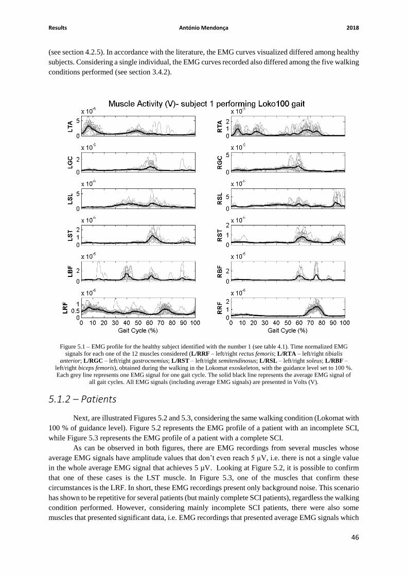
Results António Mendonça 2018
46
(see section 4.2.5). In accordance with the literature, the EMG curves visualized differed among healthy
subjects. Considering a single individual, the EMG curves recorded also differed among the five walking
conditions performed (see section 3.4.2).
5.1.2 – Patients
Next, are illustrated Figures 5.2 and 5.3, considering the same walking condition (Lokomat with
100 % of guidance level). Figure 5.2 represents the EMG profile of a patient with an incomplete SCI,
while Figure 5.3 represents the EMG profile of a patient with a complete SCI.
As can be observed in both figures, there are EMG recordings from several muscles whose
average EMG signals have amplitude values that don’t even reach 5 µV, i.e. there is not a single value
in the whole average EMG signal that achieves 5 µV. Looking at Figure 5.2, it is possible to confirm
that one of these cases is the LST muscle. In Figure 5.3, one of the muscles that confirm these
circumstances is the LRF. In short, these EMG recordings present only background noise. This scenario
has shown to be repetitive for several patients (but mainly complete SCI patients), regardless the walking
condition performed. However, considering mainly incomplete SCI patients, there were also some
muscles that presented significant data, i.e. EMG recordings that presented average EMG signals which
Figure 5.1 – EMG profile for the healthy subject identified with the number 1 (see table 4.1). Time normalized EMG
signals for each one of the 12 muscles considered (L/RRF – left/right rectus femoris; L/RTA – left/right tibialis
anterior; L/RGC – left/right gastrocnemius; L/RST – left/right semitendinosus; L/RSL – left/right soleus; L/RBF –
left/right biceps femoris), obtained during the walking in the Lokomat exoskeleton, with the guidance level set to 100 %.
Each grey line represents one EMG signal for one gait cycle. The solid black line represents the average EMG signal of
all gait cycles. All EMG signals (including average EMG signals) are presented in Volts (V).

Results António Mendonça 2018
47
represented, in fact, some kind of muscular activity (in Volts, as can be seen in Figures 5.2). In short,
basically both patients’ groups constituted the main reason to construct an algorithm capable of
eliminating EMG artifacts (see section 4.2.5).
Figure 5.2 – EMG profile for the incomplete SCI patient identified with the number 1 (see table 4.2). Time normalized
EMG signals for each one of the 12 muscles considered (L/RRF – left/right rectus femoris; L/RTA – left/right tibialis
anterior; L/RGC – left/right gastrocnemius; L/RST – left/right semitendinosus; L/RSL – left/right soleus; L/RBF –
left/right biceps femoris), obtained during the walking in the Lokomat exoskeleton, with the guidance level set to 100 %.
Each grey line represents one EMG signal for one gait cycle. The solid black line represents the average EMG signal of
all gait cycles. All EMG signals (including average EMG signals) are presented in Volts (V).

Results António Mendonça 2018
48
5.2 – Elimination of EMG Artifacts
Next, are presented two tables (one table for healthy subjects and one table for patients) that
exhibit the number of muscles (EMG curves) compromised per walking condition for each healthy
subject/patient. Besides that, these tables also indicate, between parenthesis, which muscles (EMG
signals) are compromised.
5.2.1 – Healthy Subjects
Figure 5.3 – EMG profile for the complete SCI patient identified with the number 6 (see table 4.3). Time normalized
EMG signals for each one of the 12 muscles considered (L/RRF – left/right rectus femoris; L/RTA – left/right tibialis
anterior; L/RGC – left/right gastrocnemius; L/RST – left/right semitendinosus; L/RSL – left/right soleus; L/RBF –
left/right biceps femoris), obtained during the walking in the Lokomat exoskeleton, with the guidance level set to 100 %.
Each grey line represents one EMG signal for one gait cycle. The solid black line represents the average EMG signal of
all gait cycles. All EMG signals (including average EMG signals) are presented in Volts (V).
Table 5.1 – Number of muscles (EMG curves) compromised per walking condition (OverC – self-paced over-ground
walking; OverM – metronome over-ground walking; Loko50 – Lokomat guided walking, with the guidance level set to
50 %; Loko100 – Lokomat guided walking, with the guidance level set to 100 %; GT – Gait Trainer GT1 guided
walking) for each healthy subject. Muscles’ names indicated between parenthesis are abbreviated (see the nomenclature
in the captions of figures 5.1, 5.2 and 5.3).

Results António Mendonça 2018
49
Walking
Condition
Healthy
Walker
OverC OverM Loko50 Loko100 GT Total per
subject
1 1 (RRF) 3 (RBF; LRF;
RRF)
6 (LGC; LST;
RST; LBF;
LRF; RRF)
1 (LRF)
6 (LTA;
RTA; LGC;
RGC; RSL;
RST)
17
2 2 (LRF; RRF) 3 (RBF; LRF;
RRF) 1 (LBF)
3 (RST; LBF;
RRF)
7 (LGC;
RGC; LSL;
LST; RST;
LBF; RBF)
16
3 0 0 1 (LRF) 0
7 (LGC;
LSL; RSL;
LST; RST;
LBF; LRF)
8
4 0 2 (LRF; RRF) 3 (LTA; LBF;
RRF)
9 (LTA; LGC;
RGC; LSL;
LST; LBF;
RBF; LRF;
RRF)
8 (LTA;
LGC; RGC;
LSL; RSL;
LST; RST;
RBF)
22
5 0 2 (LRF; RRF) 4 (LST; LBF;
LRF; RRF)
5 (LGC; LST;
LBF; LRF;
RRF)
5 (LGC;
LST; RST;
LBF; RBF)
16
6 0 0 4 (LTA; RTA;
RST; RBF)
3 (LTA; RTA;
RST)
4 (LGC;
RGC; LBF;
RBF)
11
7 0 5 (LST; RST;
RBF; LRF;
RRF)
6 (RGC; RST;
LBF; RBF;
LRF; RRF)
8 (LGC; RGC;
LST; RST;
LBF; RBF;
LRF; RRF)
9 (LTA;
LGC; RGC;
RSL; LST;
RST; RBF;
LRF; RRF)
28
8 2 (RBF; RRF) 1 (RST) 3 (LTA; RSL;
LRF) 1 (LRF)
8 (LTA;
RTA; LGC;
RGC; LSL;
RSL; RST;
RBF)
15
9 0 1 (RRF) 4 (RTA; LGC;
LRF; RRF)
4 (RTA; LGC;
LRF; RRF)
5 (RGC;
LSL; RSL;
RST; LRF)
14
10
7 (LTA; RGC;
RSL; RST;
RBF; LRF;
RRF)
3 (LST; LRF;
RRF)
7 (RTA; LGC;
RGC; RST;
LBF; RBF;
RRF)
7 (LGC; RGC;
LSL; LST;
RST; RBF;
RRF)
10 (LGC;
RGC; LSL;
RSL; LST;
RST; LBF;
RBF; LRF;
RRF)
34
Total per
condition 12 20 39 41 69 181
Table 5.1 indicates between parenthesis, for each healthy subject, according to each walking
condition, which precise muscles will not be considered on a further analysis. Compromised muscles’

Results António Mendonça 2018
50
names are abbreviated, but the nomenclature for each name can be consulted in the captions of Figures
5.1, 5.2 and 5.3.
5.2.2 – Patients
Walking Condition
Patient
Loko50 Loko100 GT Total per
patient
1 (Incomplete SCI) 9 (LGC; RGC; LSL;
LST; RST; LBF;
RBF; LRF; RRF)
11 (all muscles,
except LTA) 12 (all muscles) 32
2 (Incomplete SCI) 8 (LTA; RTA; LGC;
RGC; RSL; LBF;
RBF; LRF)
12 (all muscles)
7 (LTA; RTA; LGC;
RGC; LSL; RSL;
LBF)
27
3 (Incomplete SCI) 8 (LTA; RTA; LGC;
LSL; RSL; RST;
LRF; RRF)
5 (LTA; LSL; RSL;
RST; LRF)
10 (LTA; RTA; LGC;
RGC; LSL; RSL;
LST; RST; LBF;
RBF)
23
4 (Incomplete SCI) 6 (LTA; RTA; LST;
RST; RBF; LRF)
5 (RTA; LST; RST;
RBF; LRF)
11 (all muscles,
except RRF) 22
5 (Incomplete SCI) 2 (LTA; LGC) 3 (LTA; LST; RRF) 3 (LTA; RSL; LBF) 8
6 (Complete SCI) 12 (all muscles) 12 (all muscles)
10 (LTA; RTA; LGC;
RGC; LSL; RSL;
LST; RST; RBF;
RRF)
34
7 (Complete SCI)
10 (RTA; LGC;
RGC; LSL; RSL;
LST; RST; LBF;
RBF; LRF)
11 (all muscles,
except RRF)
11 (all muscles,
except RRF) 32
8 (Complete SCI) 11 (all muscles,
except RTA)
11(all muscles, except
RST)
11 (all muscles,
except LRF) 33
9 (Complete SCI) 12 (all muscles) 12 (all muscles) 12 (all muscles) 36
Total per
condition
78 (Incomplete SCI: 33)
(Complete SCI: 45)
82 (Incomplete SCI: 36)
(Complete SCI: 46)
87 (Incomplete SCI: 43)
(Complete SCI: 44)
248 (Incomplete: 113)
(Complete: 135)
Considering only the complete SCI patients referred in Table 5.2, a total of 144 EMG curves
was obtained (4 complete SCI patients * 3 walking conditions * 12 muscles). Unfortunately, after the
implementation of the excursion’s threshold (fixed at 6.5 µV) of the 144 EMG curves displayed only 9
(144 initial EMG curves – 135 compromised EMG curves) remained available for further analysis.
Therefore, it was agreed to discard and not include all data related to complete SCI patients on further
analysis. This means that, only data referring to incomplete SCI patients will be considered in the
following subchapters of this dissertation. Considering only incomplete SCI patients, according to Table
5.2, for the Gait Trainer GT1 guided walking there were three muscles compromised for all incomplete
SCI patients. The compromised muscles are: left tibialis anterior, right soleus and left biceps femoris.
Therefore, for the Gait Trainer GT1 guided walking these 3 muscles will not be included and will be
seen as a gap on any future analysis.
Table 5.2 indicates between parenthesis, for each patient according to each walking condition,
which precise muscles will not be considered on further analysis. Compromised muscles’ names are
Table 5.2 – Number of muscles (EMG curves) compromised per walking condition (Loko50 – Lokomat guided walking,
with the guidance level set to 50 %; Loko100 – Lokomat guided walking, with the guidance level set to 100 %; GT – Gait
Trainer GT1 guided walking) for each patient. Muscles’ names indicated between parenthesis are abbreviated (see the
nomenclature in the captions of figures 5.1, 5.2 and 5.3).

Results António Mendonça 2018
51
abbreviated, but the nomenclature for each name can be consulted in the captions of Figures 5.1, 5.2 and
5.3.
5.3 – Normalized EMG Curves
Next, two illustrative EMG profiles are presented (Figures 5.4 and 5.5), each one containing 12
normalized EMG curves. One of the EMG profiles presented concerns a healthy subject (in this case the
healthy subject identified with the number 2), while the other corresponds to an incomplete SCI patient
(in this case, the patient identified with the number 5). EMG profiles, containing normalized data, were
obtained for all healthy subjects/ incomplete SCI patients. Normalized EMG profiles for the remaining
healthy subjects/ incomplete SCI patients can be found, respectively, in Annexes A) and B).
As can be seen is Figures 5.4 and 5.5, as well in figures found in Annexes A) and B), each
walking condition is represented by a specific color. The color scheme, presented as a color caption, for
all walking conditions can be found and consulted in the bottom of each figure. Since, healthy subjects
performed more walking conditions than patients, the color scheme used for healthy subjects is different
from the one used for patients. Additionally, in each figure is presented, for each walking condition, the
estimate of the stance phase’s duration, previously calculated, for the right and left leg (consult section
4.2.7). Each estimate is represented by a dashed line which is colored in accordance with the respective
walking condition.
Figure 5.4 – Normalized EMG profile for the healthy subject identified with the number 2 (see table 4.1). Time and
amplitude normalized EMG signals for each one of the 12 muscles considered (muscles’ names can be consulted in the
captions of Figures 5.1, 5.2 and 5.3). Each solid colored line represents the normalized average EMG signal of a specific
walking condition. According to the color caption (found in the bottom of the figure), black represents the Self-Paced
Over-Ground walking (OverC), blue represents the Metronome Over-Ground Walking (OverM), red represents the
Lokomat guided walking with the guidance level set to 50 % (Loko50), purple represents the Lokomat guided walking
with the guidance level adjusted to 100 % (Loko100) and green represents the Gait Trainer guided walking (GT). Each
dashed line represents the estimate of the stance phase’s duration of a specific walking condition and is colored in
accordance with the corresponding walking condition.
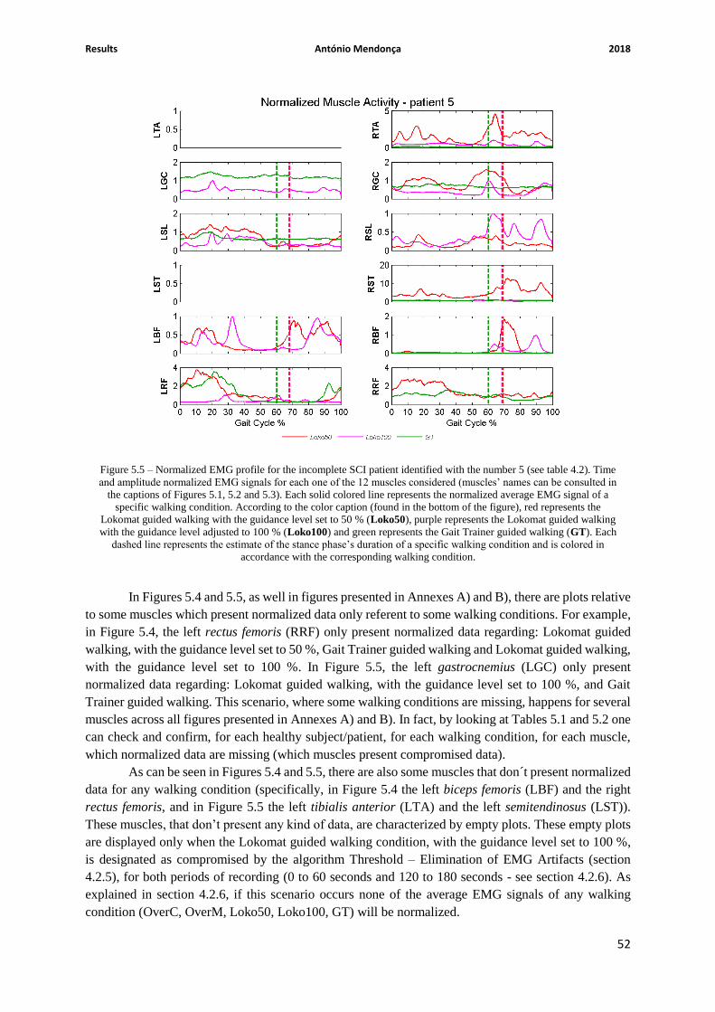
Results António Mendonça 2018
52
In Figures 5.4 and 5.5, as well in figures presented in Annexes A) and B), there are plots relative
to some muscles which present normalized data only referent to some walking conditions. For example,
in Figure 5.4, the left rectus femoris (RRF) only present normalized data regarding: Lokomat guided
walking, with the guidance level set to 50 %, Gait Trainer guided walking and Lokomat guided walking,
with the guidance level set to 100 %. In Figure 5.5, the left gastrocnemius (LGC) only present
normalized data regarding: Lokomat guided walking, with the guidance level set to 100 %, and Gait
Trainer guided walking. This scenario, where some walking conditions are missing, happens for several
muscles across all figures presented in Annexes A) and B). In fact, by looking at Tables 5.1 and 5.2 one
can check and confirm, for each healthy subject/patient, for each walking condition, for each muscle,
which normalized data are missing (which muscles present compromised data).
As can be seen in Figures 5.4 and 5.5, there are also some muscles that don´t present normalized
data for any walking condition (specifically, in Figure 5.4 the left biceps femoris (LBF) and the right
rectus femoris, and in Figure 5.5 the left tibialis anterior (LTA) and the left semitendinosus (LST)).
These muscles, that don’t present any kind of data, are characterized by empty plots. These empty plots
are displayed only when the Lokomat guided walking condition, with the guidance level set to 100 %,
is designated as compromised by the algorithm Threshold – Elimination of EMG Artifacts (section
4.2.5), for both periods of recording (0 to 60 seconds and 120 to 180 seconds - see section 4.2.6). As
explained in section 4.2.6, if this scenario occurs none of the average EMG signals of any walking
condition (OverC, OverM, Loko50, Loko100, GT) will be normalized.
Figure 5.5 – Normalized EMG profile for the incomplete SCI patient identified with the number 5 (see table 4.2). Time
and amplitude normalized EMG signals for each one of the 12 muscles considered (muscles’ names can be consulted in
the captions of Figures 5.1, 5.2 and 5.3). Each solid colored line represents the normalized average EMG signal of a
specific walking condition. According to the color caption (found in the bottom of the figure), red represents the
Lokomat guided walking with the guidance level set to 50 % (Loko50), purple represents the Lokomat guided walking
with the guidance level adjusted to 100 % (Loko100) and green represents the Gait Trainer guided walking (GT). Each
dashed line represents the estimate of the stance phase’s duration of a specific walking condition and is colored in
accordance with the corresponding walking condition.
Results António Mendonça 2018
53
As can be seen in Annex B), Figure 5.24, the normalized EMG profile of the incomplete SCI
patient identified with the number 2 is comprised of 12 empty plots. This means that the scenario
described in the previous paragraph had occurred for all 12 muscles considered. In fact, this result can
be anticipated only by looking at Table 5.2.
5.4 – Average Activation Levels
Next, are presented, through error bars, the average activation levels (with the respective
standard deviations) of both healthy subjects and incomplete SCI patients for each muscle, considering
each walking condition. Since, the average activation levels are calculated based on the normalized
curves, previously obtained (section 5.3), they do not present a unit of measure, i.e. these average
activation levels are dimensionless (they represent normalized RMS values). As referred in section 4.2.8,
the average activation levels were calculated, separately, for the stance and swing phases, and
considering additionally the entire gait cycle. So, the average activation levels (average RMS values)
given below are, for both healthy subjects and patients, referent to one of the phases mentioned above.
The three first figures (Figures 5.6., 5.7 and 5.8) are relative to healthy subjects. Figures 5.9, 5.10 and
5.11 are relative to incomplete SCI patients. Figures 5.6 and 5.9 are referent to the whole gait cycle.
Figures 5.7 and 5.10 are referent to the stance phase. Figures 5.8 and 5.11 are referent to the swing
phase. To complement the graphical information displayed below, in Annexes C) and D) are presented
tables (Tables 5.7, 5.8, 5.9, 5.11, 5.12 and 5.13) with the average RMS values (with the respective
standard deviations shown between parenthesis) for each muscle, considering each walking condition.
Again, each table presented is referent to one of the phases mentioned above (entire gait cycle, stance
phase and swing phase). The Annex C), in which are presented Tables 5.7, 5.8 and 5.9, is exclusively
dedicated to healthy subjects and the Annex D), where Tables 5.11, 5.12 and 5.13 are presented, is
exclusively dedicated to incomplete SCI patients. Also, in Annexes C) and D) are presented two tables,
Tables 5.10 and 5.14, that contain, respectively for healthy subjects and incomplete SCI patients, the
RMS values referring to the muscles that present abnormal results during the performance of a specific
walking condition.
As can be noted in Figures 5.6 to 5.11, for each muscle, each walking condition is represented
by a specific color. The color scheme, presented as a color caption, can be consulted in the bottom of
each of the figures upper mentioned. As referred in section 5.3, the color scheme used for patients is
different from the one used for healthy subjects (the reason is also described in section 5.3).

Results António Mendonça 2018
54
5.4.1 – Healthy Subjects
Figure 5.6 – Average activation levels, with the respective standard deviation, over all healthy subjects (clinically
described in table 4.1), for each muscle, considering each walking condition – considering the whole gait cycle. The
name of each one of the 12 muscles considered can be consulted in the caption of Figure 5.4. The method used to obtain
such average RMS values is described in section 4.6.8. Each colored bar represents, for each muscle, the average
activation level of a specific walking condition. As can be seen in the color caption (found in the bottom of the figure),
black represents the Self-Paced Over-Ground walking (OverC), blue represents the Metronome Over-Ground Walking
(OverM), red represents the Lokomat guided walking with the guidance level set to 50 % (Loko50), purple represents
the Lokomat guided walking with the guidance level adjusted to 100 % (Loko100) and green represents the Gait Trainer
guided walking (GT).

Results António Mendonça 2018
55
Figure 5.7 – Average activation levels, with the respective standard deviation, over all healthy subjects (clinically
described in table 4.1), for each muscle, considering each walking condition – considering only the stance phase. The
name of each one of the 12 muscles considered can be consulted in the caption of Figure 5.4. The method used to obtain
such average RMS values is described in section 4.6.8. Each colored bar represents, for each muscle, the average
activation level of a specific walking condition. The color scheme used for representing each walking condition is equal
to the one that is used in Figure 5.6.
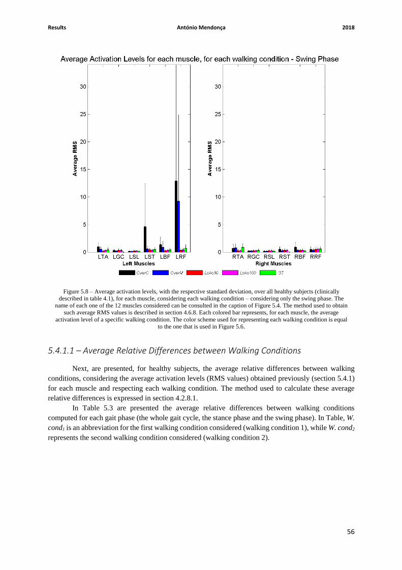
Results António Mendonça 2018
56
5.4.1.1 – Average Relative Differences between Walking Conditions
Next, are presented, for healthy subjects, the average relative differences between walking
conditions, considering the average activation levels (RMS values) obtained previously (section 5.4.1)
for each muscle and respecting each walking condition. The method used to calculate these average
relative differences is expressed in section 4.2.8.1.
In Table 5.3 are presented the average relative differences between walking conditions
computed for each gait phase (the whole gait cycle, the stance phase and the swing phase). In Table, W.
cond1 is an abbreviation for the first walking condition considered (walking condition 1), while W. cond2
represents the second walking condition considered (walking condition 2).
Figure 5.8 – Average activation levels, with the respective standard deviation, over all healthy subjects (clinically
described in table 4.1), for each muscle, considering each walking condition – considering only the swing phase. The
name of each one of the 12 muscles considered can be consulted in the caption of Figure 5.4. The method used to obtain
such average RMS values is described in section 4.6.8. Each colored bar represents, for each muscle, the average
activation level of a specific walking condition. The color scheme used for representing each walking condition is equal
to the one that is used in Figure 5.6.

Results António Mendonça 2018
57
Average Relative Differences (%)
Gait Phase
𝑊. 𝑐𝑜𝑛𝑑1 − 𝑊. 𝑐𝑜𝑛𝑑2
𝑊. 𝑐𝑜𝑛𝑑1∗ 100%
Whole Gait
Cycle Stance Phase Swing Phase
𝑂𝑣𝑒𝑟𝐶 − 𝑂𝑣𝑒𝑟𝑀
𝑂𝑣𝑒𝑟𝐶∗ 100% 38.69 % 39.25 % 41.42 %
𝑂𝑣𝑒𝑟𝐶 − 𝐿𝑜𝑘𝑜50
𝑂𝑣𝑒𝑟𝐶∗ 100% 84.48 % 84.90 % 84.12 %
𝑂𝑣𝑒𝑟𝐶 − 𝐿𝑜𝑘𝑜100
𝑂𝑣𝑒𝑟𝐶∗ 100% 86.53 % 87.36 % 83.71 %
𝑂𝑣𝑒𝑟𝐶 − 𝐺𝑇
𝑂𝑣𝑒𝑟𝐶∗ 100% 84.89 % 88.32 % 82.06 %
𝑂𝑣𝑒𝑟𝑀 − 𝐿𝑜𝑘𝑜50
𝑂𝑣𝑒𝑟𝑀∗ 100% 74.69 % 75.14 % 72.89 %
𝑂𝑣𝑒𝑟𝑀 − 𝐿𝑜𝑘𝑜100
𝑂𝑣𝑒𝑟𝑀∗ 100% 78.03 % 79.19 % 72.19 %
𝑂𝑣𝑒𝑟𝑀 − 𝐺𝑇
𝑂𝑣𝑒𝑟𝑀∗ 100% 75.36 % 80.77 % 69.38 %
𝐿𝑜𝑘𝑜50 − 𝐿𝑜𝑘𝑜100
𝐿𝑜𝑘𝑜50∗ 100% 13.20 % 16.31 % -2.56 %
𝐿𝑜𝑘𝑜50 − 𝐺𝑇
𝐿𝑜𝑘𝑜50∗ 100% 2.64 % 22.66 % -12.95 %
𝐿𝑜𝑘𝑜100 − 𝐺𝑇
𝐿𝑜𝑘𝑜100∗ 100% -12.15 % -12.15 % -10.13 %
Table 5.3 – Healthy Subjects: Average relative differences between walking conditions, for each gait phase (the whole
gait cycle, the stance phase and the swing phase), considering the average activation levels obtained for each muscle and
respecting each walking condition.

Results António Mendonça 2018
58
5.4.2 – Incomplete SCI Patients
Figure 5.9 – Average activation levels, with the respective standard deviation, over all incomplete SCI patients (clinically
described in table 4.2), for each muscle, considering each walking condition – considering the whole gait cycle. The
name of each one of the 12 muscles considered can be consulted in the caption of Figure 5.5. The method used to obtain
such average RMS values is described in section 4.6.8. Each colored bar represents, for each muscle, the average
activation level of a specific walking condition. As can be seen in the color caption (found in the bottom of the figure),
red represents the Lokomat guided walking with the guidance level set to 50 % (Loko50), purple represents the Lokomat
guided walking with the guidance level adjusted to 100 % (Loko100) and green represents the Gait Trainer guided
walking (GT).

Results António Mendonça 2018
59
Figure 5.10 – Average activation levels, with the respective standard deviation, over all incomplete SCI patients
(clinically described in table 4.2), for each muscle, considering each walking condition – considering only the stance
phase. The name of each one of the 12 muscles considered can be consulted in the caption of Figure 5.5. The method
used to obtain such average RMS values is described in section 4.6.8. Each colored bar represents, for each muscle, the
average activation level of a specific walking condition. The color scheme used for representing each walking condition
is equal to the one that is used in Figure 5.9.

Results António Mendonça 2018
60
5.4.2.1 – Average Relative Differences between Walking Conditions
Next are presented, for incomplete SCI patients, the average relative differences between
walking conditions, considering the average activation levels (RMS values) obtained previously (section
5.4.2) for each muscle and respecting each walking condition. The method used to calculate these
average relative differences is explained in section 4.2.8.1.
In Table 5.4 are presented the average relative differences between walking conditions
computed for each gait phase (the whole gait cycle, the stance phase and the swing phase). In Table, W.
cond1 is an abbreviation for the first walking condition considered (walking condition 1), while W. cond2
represents the second walking condition considered (walking condition 2).
Figure 5.11 – Average activation levels, with the respective standard deviation, over all incomplete SCI patients
(clinically described in table 4.2), for each muscle, considering each walking condition – considering only the swing
phase. The name of each one of the 12 muscles considered can be consulted in the caption of Figure 5.5. The method
used to obtain such average RMS values is described in section 4.6.8. Each colored bar represents, for each muscle, the
average activation level of a specific walking condition. The color scheme used for representing each walking condition
is equal to the one that is used in Figure 5.9.

Results António Mendonça 2018
61
Average Relative Differences (%)
Gait Phase
𝑊. 𝑐𝑜𝑛𝑑1 − 𝑊. 𝑐𝑜𝑛𝑑2
𝑊. 𝑐𝑜𝑛𝑑1∗ 100%
Whole Gait
Cycle Stance Phase Swing Phase
𝐿𝑜𝑘𝑜50 − 𝐿𝑜𝑘𝑜100
𝐿𝑜𝑘𝑜50∗ 100% 77.42 % 73.17 % 83.47 %
𝐿𝑜𝑘𝑜50 − 𝐺𝑇
𝐿𝑜𝑘𝑜50∗ 100% 63.80 % 56.90 % 72.37 %
𝐿𝑜𝑘𝑜100 − 𝐺𝑇
𝐿𝑜𝑘𝑜100∗ 100% -60.35 % -60.65 % -67.11 %
5.5 – Average A1 Coefficients Next, are presented, through error bars, the average A1 coefficients (with the respective standard
deviations) of both healthy subjects and incomplete SCI patients for each muscle, considering each
walking condition. To complement the graphical information displayed below in Figures 5.12 and 5.13,
in Annex E) are presented tables (Tables 5.15 and 5.16) which contain the average A1 coefficient (with
the respective standard deviation shown between parenthesis) for each one of the six muscles
considered, respecting each walking condition performed. In Annex E) are also presented, through bar
plots, the A1 coefficients corresponding to each healthy subject/patient, for each one of the six muscles,
considering all walking conditions performed.
As can be noted in the following figures, for each walking condition performed each one of the
six muscles is represented by a specific color. The color scheme, presented as a color caption, can be
consulted in the bottom of each one of the figures displayed below. In this case, since the number of
muscles studied is the same for both healthy subjects and incomplete SCI patients, the color scheme
used for patients is equal to the one used for healthy subjects. Also, it is possible to observe in the
following figures the average A1 coefficient over all six muscles for each walking condition performed
(the average A1 coefficient per walking condition). The average A1 coefficient per walking condition is
represented, for each walking condition, by a black dashed line. The standard deviation corresponding
to each average A1 coefficient per walking condition was calculated based on the average symmetry
coefficients (average A1 coefficients) exhibited by all six muscles. The standard deviations respective to
the average A1 coefficients per walking condition can be consulted in the tables expressed in Annex E).
Each table displayed in Annex E) indicate all standard deviations between parenthesis.
5.5.1 – Healthy Subjects
In Figure 5.12, are presented, for healthy subjects, the average A1 coefficients (with the
respective standard deviations) for each muscle considering each walking condition.
Table 5.4 – Incomplete SCI Patients: Average relative differences between walking conditions, for each gait phase (the
whole gait cycle, the stance phase and the swing phase), considering the average activation levels obtained for each
muscle and respecting each walking condition.

Results António Mendonça 2018
62
5.5.1.1 – Average Symmetry Discrepancies
Next, Table 5.5 displays the average symmetry discrepancy, regarding healthy subjects, for each
one of the six muscles (TA, GC, SL, ST, BF and RF) studied, for each one of the walking conditions
performed (OverC, OverM, Loko50, Loko100 and GT – consult caption of Table 5.1). In Table 5.5 the
average symmetry discrepancies per walking condition are also displayed, as well as the respective
standard deviations (presented between parenthesis). The standard deviation per walking condition,
presented between parenthesis for each walking condition, was calculated based on the average
symmetry discrepancies exhibited by all six muscles. The method used to calculate these average
symmetry discrepancies is fully explained and described in section 4.2.9.1. All data used in equation
(4.7), to calculate such average symmetry discrepancies, are displayed in Annex E), Table 5.15.
Figure 5.12 – Average A1 coefficients, with the respective standard deviation, over all healthy subjects (clinically
described in Table 4.1), for each walking condition performed, considering each muscle. The name of each one of the 5
walking conditions considered can be consulted in the caption of Table 5.1. The method used to obtain such average A1
coefficients is described in section 4.6.9. Each colored bar represents, for each walking condition, the average A1
coefficient of a specific muscle. As can be seen in the color caption (found in the bottom of the figure), blue represents
the tibialis anterior (TA), cyan represents the gastrocnemius (GC), green represents the soleus (SL), purple represents
the semitendinosus (ST), red represents the biceps femoris (BF) and black represents the rectus femoris (RF). Each one
of the five black dashed lines represents the average A1 coefficient over all six muscles for each one of the walking
conditions performed.

Results António Mendonça 2018
63
Walking
Condition
Muscle
OverC OverM Loko50 Loko100 GT
TA 6 % 9 % 8 % 14 % 4 %
GC 2 % 7 % 2 % NaN NaN
SL 8 % 9 % 14 % 21 % 13 %
ST 6 % 16 % 7 % 10 % 13 %
BF 20 % 26 % 11 % 15 % 17 %
RF 16 % 34 % 38 % NaN 2 %
Average
Symmetry
Discrepancy
per Walking
Condition (standard
deviation)
9.67 % (6.86 %)
16.83 % (10.94 %)
13.33 % (12.74 %)
15.00 % (4.55 %)
9.80 % (6.46 %)
5.5.2 – Incomplete SCI Patients
In Figure 5.13, are presented, for incomplete SCI patients, the average A1 coefficients (with the
respective standard deviations) for each muscle considering each walking condition.
5.5.2.1 – Average Symmetry Discrepancies
Next, is also presented Table 5.6, which displays the average symmetry discrepancy, regarding
incomplete SCI patients, for each one of the six muscles (TA, GC, SL, ST, BF and RF) studied, for each
one of the walking conditions performed (Loko50, Loko100 and GT – consult caption of Table 5.2). In
Table 5.6 are also displayed the average symmetry discrepancies per walking condition, as well as the
respective standard deviations (presented between parenthesis). The standard deviation per walking
condition, presented between parenthesis for each walking condition, was calculated based on the
average symmetry discrepancies exhibited by all six muscles. The method used to calculate these
average symmetry discrepancies is fully explained and described in section 4.2.9.1. All data used in
equation (4.7), to calculate such average symmetry discrepancies, are displayed in Annex E), Table 5.16.
Table 5.5 – Average symmetry discrepancies, regarding healthy subjects, for each one of the walking conditions
performed, considering each one of the six muscles studied. All data used to calculate such average symmetry
discrepancies are displayed in Annex E), Table 5.15. The last row indicates the average symmetry discrepancy per
walking condition, for each one of the walking conditions performed.

Results António Mendonça 2018
64
Walking
Condition
Muscle
Loko50 Loko100 GT
TA NaN NaN NaN
GC NaN NaN NaN
SL NaN NaN NaN
ST NaN NaN 16 %
BF NaN NaN NaN
RF 22 % NaN 11 % Average
Symmetry
Discrepancy
per Walking
Condition (standard
deviation)
22.00 % (0.00 %)
NaN 13.50 % (3.54 %)
Figure 5.13 – Average A1 coefficients, with the respective standard deviation, over all incomplete SCI patients (clinically
described in Table 4.2), for each walking condition performed, considering each muscle. The name of each one of the 3
walking conditions considered can be consulted in the caption of Table 5.2. The method used to obtain such average A1
coefficients is described in section 4.6.9. Each colored bar represents, for each walking condition, the average A1
coefficient of a specific muscle. The color scheme for each muscle can be consulted in caption of Figure 5.12 Each black
dashed line represents the average A1 coefficient over all six muscles for each one of the walking conditions performed.
Table 5.6 – Average symmetry discrepancies, regarding incomplete SCI patients, for each one of the walking conditions
performed, considering each one of the six muscles studied. All data used to calculate such average symmetry
discrepancies are displayed in Annex E), Table 5.16. The last row indicates the average symmetry discrepancy per
walking condition, for each one of the walking conditions performed.

Discussion António Mendonça 2018
65
CHAPTER 6 – DISCUSSION
This chapter is dedicated to the discussion of the results previously obtained in Chapter 5.
6.1 – Elimination of EMG Artifacts
According to Tables 5.1 and 5.2, the total number of compromised EMG curves is bigger for
the 9 patients (248 EMG curves from 324 EMG curves available) than for the 10 healthy subjects (181
EMG curves from 600 EMG curves available). This was expected, since an injured spinal cord loses
some or all abilities to send and receive messages from the brain to the body’s system that controls
sensory and motor functions.
Since, an injured spinal cord loses, completely or incompletely, the ability to convey messages
to or from the brain, motor and sensory functions of inferior limb muscles below the level of injury will
depend if the injury is classified as complete or incomplete. In fact, according to Table 5.2, the total
number of compromised EMG curves is higher for the 4 complete SCI patients (135 EMG curves from
a total of 145) than for the 5 incomplete SCI patients (113 EMG curves from a total of 180). Besides
that, it is possible to verify that the number of compromised EMG curves of any incomplete SCI patient,
except for the first patient (number 1), is smaller than the one exhibited by any complete SCI patient.
These results obtained for both groups of patients are sustained by what is expressed in Tables 4.2 and
4.3, namely the AIS grade. All complete SCI patients described in Table 4.3 and presented in Table 5.2
were classified with the grade A (the most severe level of SCI) in the AIS scale. In part, this classification
for all complete SCI patients can explain the high number of EMG curves neglected. As referred in
Chapter 5, regarding complete SCI patients, since almost EMG curves available are compromised, one
may infer that all EMG data relative to complete SCI patients might not be entirely trustworthy. In fact,
all EMG data referring to the 9 non-compromised muscles may only reflect spasticity or the occurrence
of reflexes (involuntary reactions) that are processed directly in spinal cord, without being perceived by
the cerebral cortex, i.e. without the person being consciously aware of the stimulus. Based on that, it
was agreed to discard, from any subsequent analysis, all data relative to complete SCI patients.
Regarding incomplete SCI patients, 3 of them were classified with the grade D (the least severe level of
SCI) and the other 2 were classified with the grade C. Consulting Table 5.2, one can confirm that
incomplete SCI patients classified with the grade D are the ones that have less EMG curves rejected. On
the other hand, the incomplete SCI patient that presented the highest number of compromised EMG
curves was the first patient (number 1) with 32 signals compromised. This agrees with what is expressed
in section 2.3.3. According to the description of the AIS scale, the grade C means that some muscle
movement (motor function) is preserved below the neurologic level of injury, but more than half of key
muscles below the level of injury cannot move against gravity. According to the same description, the
grade D claims that motor function is preserved below the neurologic level of injury, and most key
muscles below the level of injury are strong enough to move against gravity.
Regarding healthy subjects, in Table 5.1 is possible to verify that the tenth subject (number 10)
was the one that presented more compromised EMG curves (34). This could happen due to a bad
adaptation of the subject to the walking conditions in question, or to the detachment of some wireless
surface sensors during an initial stage of the procedure. This is supported by the fact that the tenth subject
displayed a high number of compromised curves for basically all walking conditions performed, except
for the over-ground walking guided by a metronome (OverM). Another important aspect to point out in
Table 5.1 is the total number of EMG curves compromised per walking condition. The conditions that
presented the smallest number of compromised curves were the self-paced over-ground walking (12)
and the over-ground walking guided by a metronome (20). The results involving these two walking
Discussion António Mendonça 2018
66
conditions were expected, since these are the best approximations of a gait performed in a natural
environment.
Looking at Tables 5.1 and 5.2, one can observe that the Gait Trainer GT1 guided walking was
the condition that presented more compromised curves, for both healthy subjects and patients. The total
number of compromised curves displayed by all healthy subjects was 69. The total number of
compromised curves exhibited by all patients was 87. Looking at Table 5.1, it is possible to note that
the total number of compromised curves presented by the GT walking condition is much higher than the
one presented by any other walking condition. Additionally, one can verify that each healthy subject
presents a high number of compromised curves for the GT walking condition. Consulting Table 5.2, it
is possible to notice that, although the distribution of the number of compromised curves is, for all
walking conditions, more uniform for patients (especially complete SCI patients) than for healthy
subjects, the Gait Trainer GT1 guided walking is still the condition that presents the highest total number
of compromised curves. Besides that, each patient, with exception of the fifth patient, exhibits a high
number of compromised curves for the GT walking condition. The possible reasons why this scenario
occurred for both healthy subjects and patients are the following:
a) Fatigue – since all walking conditions were performed on the same day, for most subjects,
and GT walking condition was the last to be performed, considering both healthy subjects
and patients. In case of patients, the difficulties in mobility required an additional effort that
promoted even more the fatigue.
b) Bad adaptation – during the experimental setup of the Gait Trainer GT1 session, the
adaptation of some subjects to a new harness was not easy, and in some cases, had forced
the reconfiguration of the sensors’ placement. Additionally, the long period separating the
first from the last session, as well as the change of location (RAR devices weren’t all in the
same room) between sessions had caused in most subjects the detachment of sensors.
c) Gait Trainer GT1 is an end-effector type RAR device that suffers from limited control of
the proximal joints of inferior limbs, which could result in abnormal movement patterns. In
this case, the level of support given by Gait Trainer GT1 to subjects is automatic, which
may not have encouraged subjects’ engagement on the task performed. Additionally,
footplates movements might have replaced entirely the motor function of some leg muscles,
which means that a subject could be performing a gait on the Gait Trainer GT1 without
intentionally activating those specific muscles.
6.2 – Normalized EMG Curves
In the context of this dissertation, the outcomes of normalization are considered satisfactory
when the number of compromised EMG curves corresponding to the Lokomat guided walking, with the
guidance level set to 100 %, is low. In practical terms, this corresponds, in the presentation of a figure
(for example Figures 5.4 and 5.5), to a low number of empty plots. The optimal circumstances
correspond to cases where figures don’t present a single empty plot. As referred in section 5.3, these
empty plots are displayed only when the Lokomat guided walking condition, with the guidance level set
to 100 %, is designated as compromised by the algorithm Threshold – Elimination of EMG Artifacts
(section 4.2.5), for both periods of recording (0 to 60 seconds and 120 to 180 seconds - see section
4.2.6). On the other hand, there are some cases where the average EMG signal, corresponding to the
Lokomat guided walking, referring to the first 60 seconds period of recording (from 0 to 60 seconds)
was used, which could lead to some discrepancies between the information displayed in Figures 5.4 and

Discussion António Mendonça 2018
67
5.5, as well as in Figures 5.14 to 5.26, and the information that is presented in Tables 5.1 and 5.2. For
example, in Figure 5.4 are presented only 2 empty plots, but consulting Table 5.2 it is possible to note
that there are 3 compromised curves for the Lokomat guided walking, with the guidance level set to 100
%. This means that the information presented by figures and tables previously mentioned doesn’t
necessarily have to match.
Regarding healthy subjects, looking at Figure 5.15, presented in Annex A), and confirming with
Table 5.1, the subject that presents the best outcomes in terms of normalization is the third one (subject
number 3), since he does not present a single empty plot. On the other hand, subjects that present the
worst outcomes are the fourth (subject number 4) and the seventh (subject number 7), since each one
presents 7 empty plots, as can be seen in Figures 5.16 and 5.19, presented in Annex A). Regarding
incomplete SCI patients, the one that presents the best outcomes is the fifth patient (patient number 5),
with only 2 empty plots (Figure 5.5). On the other hand, the patient that presents the worst outcomes is
the second one, since all 12 EMG curves are described by an empty plot (Figure 5.24, Annex B)).
As can be seen in Figures 5.4 and 5.5, as well as in Figure 5.14 to 5.26, the stance phase,
considering the same walking condition, is different between subjects, except for the GT walking
condition. Besides that, considering each single subject the stance phase obtained is different for each
walking condition performed. Additionally, considering each single subject, the stance phase estimated
for each single walking condition usually differs between the right and left legs. These results were
expected. In fact, the small differences shown by each subject during gait performance can be used,
somewhat like the fingerprint, as a unique characteristic element capable of identifying (distinguishing)
one specific individual in the midst of many others.
6.3 – Average Activation Levels
Regarding healthy subjects, looking at Figures 5.6 to 5.8, there are some specific muscles that
exhibit excessively high average activation levels, for some specific walking conditions, regardless the
gait phase considered (stance, swing or the entire gait cycle). The muscles and walking conditions in
question are: the left semitendinosus (LST) while performing the self-paced over-ground walking
(OverC), and the left rectus femoris (LRF) while performing the self-paced over-ground walking and
the over-ground walking guided by a metronome (OverM). In Annex C) it is presented Table 5.10,
which contains, for each gait phase considered, the RMS values corresponding to each healthy subject,
for each one of the muscles mentioned above, considering the walking conditions also above-mentioned.
Looking at Table 5.10, it is possible to note that the average RMS referring to the left rectus femoris,
for both OverC and OverM, is calculated based on the RMS values of two subjects, corresponding to
numbers 3 and 6. Since, the subject number 3 displays a huge RMS value, for each gait phase considered,
the average RMS referring to the left rectus femoris, for both OverC and OverM, assumes a value which,
compared with the remaining average RMS values, is excessively high. The big variation between the
two values used to calculate the average RMS value referring to the left rectus femoris, for both OverC
and OverM, is explicit, in Figures 5.6 to 5.8, by the high value displayed by the standard deviation. As
can be seen in Table 5.10, the average RMS value referring to the LST for the OverC, for each gait
phase considered, is calculated based on seven subjects – numbers 1, 2, 3, 4, 6, 8 and 9. The sixth and
the ninth subjects display RMS values which can be considered very high, in comparison with the values
displayed by the remaining subjects. These two values have a big influence on the value that the average
RMS value displays. In fact, these values explain the big variation, presented in Table 5.10 between
parenthesis, calculated over the seven RMS values and illustrated by a big standard deviation.
Looking at Figures 5.6 to 5.8, as well as Tables 5.7 to 5.9, presented in Annex C), it is possible
to note that some specific muscles don’t present an average RMS value for some specific walking

Discussion António Mendonça 2018
68
conditions. The muscles and walking conditions in question are: the left gastrocnemius (LGC) and the
right semitendinosus (RST) while performing the Gait Trainer GT1 guided walking (GT). The reasons
why these muscles don’t present an average value for this specific walking condition can be inferred
from Table 5.1. Looking at Table 5.1 it is possible to note that 9 of the 10 subjects have, for the GT
walking condition, the EMG curve referring to the LGC designated as compromised. Although, the
subject number 9 doesn’t have this curve designated as compromised, he has for the Lokomat guided
walking, with the guidance level set to 100 %, the EMG curve referring to the LGC designated as
compromised, for both periods of recording (0 to 60 seconds and 120 to 180 seconds), which means that
it is impossible, for this subject, to normalize data referring to the LGC. Thus, regarding the 10 healthy
subjects, it was not possible to obtain an average RMS value for the LGC, considering the GT walking
condition. Looking again at Table 5.1, one can verify that 9 of the 10 subjects have, for the Gait Trainer
guided walking, the EMG curve referring to the RST designated as compromised. Although, the subject
number 6 doesn’t have this curve designated as compromised, he has for the Lokomat guided walking,
with the guidance level set to 100 %, the EMG curve referring to the RST designated as compromised,
for both periods of recording, which means that it is impossible, for this subject, to normalize data
referring to the RST. Thus, regarding the 10 healthy subjects, it was impossible to obtain an average
RMS value for the RST considering the GT walking condition.
Regarding incomplete SCI patients, based on Figures 5.9 to 5.11, it is possible to see that some
muscles do not present a standard deviation for a specific walking condition. Tables 5.11 to 5.13 indicate
which muscles and walking conditions do not present a standard deviation. Every time a muscle does
not exhibit a standard deviation for a specific walking condition means that the calculation of the
respective average RMS value presented was based on a single patient.
As can be seen in Figures 5.9 to 5.11, as well as in Tables 5.11 to 5.13, presented in Annex D),
there are some specific muscles that exhibit excessively high average activation levels for some specific
walking conditions, regardless the gait phase considered (stance, swing or the entire gait cycle). The
muscles and walking conditions in question are: the right gastrocnemius (RGC) and the right
semitendinosus (RST) while performing the Lokomat guided walking, with the guidance level set to 50
% (Loko50). In Annex D) it is presented Table 5.14, which contains, for each gait phase considered, the
normalized RMS values corresponding to each patient, for each one of the muscles mentioned above,
considering the above-mentioned walking conditions. Looking at Table 5.14, it is possible to note that,
for each gait phase considered, the average RMS referring to the RGC for Loko50 is calculated based
on the RMS values of three patients, corresponding to numbers 3, 4 and 5. Since, the patient number 3
displays a huge value, for each gait phase considered, the average RMS referring to the RGC for Loko50
assumes a value which, compared with the remaining average RMS values, is excessively high. The big
variation, between the RMS of the third patient and the two other RMS values used to calculate the
average value, is illustrated, in Figures 5.6 to 5.8, by the high value displayed by the standard deviation.
As can be seen in Table 5.14, the calculation of the average RMS referring to the RST is based on a
single patient, the fifth one. Since, this patient displays, for each gait phase, a high RMS value, in turn
the average RMS also assumes a high value.
Looking at Figures 5.9 to 5.11, and confirming with Tables 5.11 to 5.13, presented in Annex
D), it is possible to note that some specific muscles don’t present an average RMS value for some
specific walking conditions. The muscles and walking conditions in question are: the left tibialis
anterior (LTA), the left semitendinosus (LST), the left biceps femoris (LBF) and the right soleus (RSL)
while performing the GT walking condition (GT). The reason for which the LTA, the RSL and the LBF
do not present average RMS values, exclusively for the Gait Trainer GT1 guided walking, is already
mentioned in the last part of the first paragraph of section 5.2.2 and is inferred directly from data
presented in Table 5.2. Looking at Table 5.2, it is possible to note that 3 of the 5 incomplete SCI patients
have, for the GT walking condition, the EMG curve referring to the LST designated as compromised.

Discussion António Mendonça 2018
69
Although, the other two incomplete SCI patients (numbers 2 and 5) don’t have this curve designated as
compromised, they have for the Lokomat guided walking, with the guidance level set to 100 %, the
EMG curve referring to the LST designated as compromised, for both periods of recording (0 to 60
seconds and 120 to 180 seconds), which means that it is impossible, for these two patients, to normalize
data referring to the LST. Thus, regarding all 5 incomplete SCI patients, it was not possible to obtain an
average RMS value for the LST considering the GT walking condition. On the other hand, there are
some muscles that appear to present null average RMS values for the GT walking condition. For
example, the right tibialis anterior (RTA) and the right biceps femoris (RBF) appear to present null
average activation levels for the Gait Trainer GT1 guided walking, but by consulting Tables 5.11 to
5.13, displayed in Annex D), one can confirm that these values, although close to zero, are not precisely
equal to zero.
6.3.1 – Average Relative Differences between Walking Conditions
Regarding healthy subjects, looking at Table 5.3 it is possible to note that, for each gait phase
considered (entire gait cycle, stance phase and swing phase), both over-ground walking conditions
present, in terms of activation, a large difference from the conditions performed on RAR devices.
Indeed, the largest differences presented are among over-ground walking conditions and conditions
performed on RAR devices. Considering the entire gait cycle, the largest difference presented
corresponds to the one between the OverC and the Loko100, being the difference of 86.35 %. During
stance, the largest difference corresponds to the difference between the OverC and the GT walking
condition (88.32 %). During swing, the largest difference corresponds to the difference between the
OverC and the Loko50 (84.12 %). These facts suggest that the activation levels produced by healthy
subjects while walking on RAR devices are quite different from those produced during gait performed
freely over the ground. On the other hand, looking again at Table 5.3 one can verify that the smallest
differences correspond to those among walking conditions performed on RAR devices. It can be said
that these differences, compared with the ones above-mentioned, are small, because none of them
reaches even 25 %. In fact, considering the entire gait cycle, the difference exhibited between the Loko50
and the GT walking condition is tiny, only of 2.64 %. Considering the stance phase, the lowest difference
presented has an absolute value of 12.15 % and is referent to the Loko100 and the GT walking condition.
Considering the swing phase, the smallest difference displayed has an absolute value of 2.56 % and
corresponds to the difference between the Loko50 and the Loko100. Besides that, looking at difference
between the Loko100 and the GT walking condition, it is possible to note that the global average
activation level presented by the Loko100 during the whole gait cycle, as well as during stance and
swing phases, is smaller than the global average activation level presented by the GT walking condition,
since all average relative differences present a negative signal. During the swing phase, Gait Trainer
GT1 produces a global average activation level slightly higher than the one produced by the Lokomat
exoskeleton, regardless the level of guidance chosen. In short, all these last facts suggest that, in case of
healthy subjects, RAR devices produce activations levels that are quite similar among them.
Looking at Table 5.4, it is possible to conclude that the scenario that had happened for healthy
subjects does not match with the one found for incomplete SCI patients. The average relative differences
among walking conditions performed on RAR devices are quite large, as compared to those calculated
for healthy subjects. In fact, all differences transcend the value of 50 %. It is possible to note that the
largest differences calculated are referent to the two levels of guidance selected for the Lokomat
exoskeleton (whole gait cycle – 77.42 %; stance phase – 73.17 %; swing phase – 83.47%). As happened
for healthy subjects, the global average activation level promoted by the Lokomat exoskeleton, with the
guidance level set to 100 %, is lower, although in larger proportions (the difference is substantially
amplified), than the one generated by the Gait Trainer GT1, during the entire gait cycle, as well as during

Discussion António Mendonça 2018
70
stance and swing phases. In short, these facts suggest that, in case of incomplete SCI patients, the
activation patterns delivered by RAR devices are quite different from each other’s. Regarding
incomplete SCI patients, considering a single RAR device, even the level of guidance is largely
determinant on the magnitude that the global average activation level will present, regardless the gait
phase considered. That’s why, especially in case of patients, each RAR device/level of guidance must
be analyzed separately, in order to understand which are the specific effects that each RAR device/level
of guidance has over the locomotor training.
6.4 – Average A1 Coefficients
Regarding healthy subjects, as noted in Figure 5.12, and confirming with Table 5.15 presented
in Annex E), there aren’t average A1 coefficients that present values excessively and abnormally high or
low. According to Table 5.15, there isn’t any average A1 coefficient smaller than 0.6 and bigger than
1.15. Otherwise, there are some muscles, for some specific walking conditions which do not present a
standard deviation. Table 5.15 indicates between parenthesis which are the muscles and walking
conditions that do not exhibit a standard deviation. The reason why some muscles do not present a
standard deviation is already explained in the third paragraph of section 6.3.
Looking at Figure 5.12, and confirming with Table 5.15, it is possible to note that some muscles
do not present an average A1 coefficient for specific walking conditions. The muscles and walking
conditions in question are: the gastrocnemius (GC) and the rectus femoris (RF) while performing the
Lokomat guided walking, with the guidance level set to 100 % (Loko100), and the gastrocnemius (GC)
while performing the Gait Trainer GT1 guided walking (GT). The possible reasons why these muscles
do not present data for the walking conditions mentioned are already referred in the sixth paragraph of
section 4.2.9. There are three scenarios that can explain why these results:
1. None of the subjects presented an A1 coefficient that has passed through the validation test
(section 4.2.9).
2. For the specific above-mentioned muscles and walking conditions, regarding all subjects,
at least one of the curves tested by the LFM was considered as compromised, according to
algorithm Threshold – Elimination of EMG Artifacts (section 4.2.5). This scenario,
although rare, could happen.
3. A third scenario that could explain the results referring to the above-mentioned muscles and
walking conditions consists of the conjugation of the two previous scenarios, where some
subjects had presented A1 coefficients considered as invalid, while the remaining had at least
one of the curves, tested by the LFM, designated as compromised, after the implementation
of the Threshold – Elimination of EMG Artifacts.
Looking again at Figure 5.12, it is possible to confirm that the OverC was the walking condition
that presented, in general terms, the best results regarding symmetry, since all six muscles displayed
average A1 coefficients close to 1, in a range between 0.8 and 0.98 (consult Table 5.15). In fact, by
looking at Table 5.15, the OverC is the walking condition that exhibits, for the average A1 coefficient
per walking condition, the lowest standard deviation (0.07). These results are supported by the fact that
the OverC is the walking condition that most resembles a natural gait. In practical terms, all walking
conditions presented in Figure 5.12 exhibited good results regarding symmetry, since all of them
displayed an average A1 coefficient per walking condition close to 1 (consult Table 5.15). However, is
important to emphasize that the calculation of the average A1 coefficient per walking condition of both
Loko100 and GT walking condition did not include all six muscles studied. In fact, looking at Table
5.15, the average A1 coefficient per walking condition that constitutes the best approximation of the

Discussion António Mendonça 2018
71
perfect symmetry (A1 = 1) is referent to the Loko100, however this same walking condition is also the
one that presents the biggest standard deviation (0.18). This means that, the average A1 coefficients
referring to the Loko100 are the ones that differ most from each other.
Unfortunately, regarding incomplete SCI patients, only three average A1 coefficients were
obtained, considering all walking conditions performed (Figure 5.13). Although these results can be
considered bad, they are admissible since the gait of these patients is often characterized by a temporal
and spatial asymmetry of the stepping pattern. In turn, this asymmetry is frequently a product of a
strategy adopted by incomplete SCI patients, in order to avoid pain. One of the purposes of using RAR
devices is to make incomplete SCI patients’ gait more symmetrical, but looking at Figure 5.13, this was
not what happened in the context of this study. The reasons why most muscles didn’t present any average
A1 coefficient for most walking conditions involve one of the three scenarios previously described for
healthy subjects. As noted in Figure 5.13, only three average A1 coefficients were obtained, considering
all walking conditions performed, and none of them presented a standard deviation, which means that
each average A1 coefficient obtained is referent to one specific incomplete SCI patient. The first average
A1 coefficient corresponds to the RF while performing the Loko50. The other two average coefficients
are referent to the ST and the RF while performing the GT walking condition. Looking at Figures 5.37
to 5.41, it is possible to verify that the average coefficient referring to the Loko50 corresponds to the
fifth patient. The other two average coefficients referring to the GT walking condition concern the
second patient. In short, it is possible to conclude that these abnormalities, in terms of symmetry,
displayed by incomplete SCI patients require control strategies, in response to the robotic assistance
provided by RAR devices, different from those adopted for healthy subjects.
6.4.1 – Average Symmetry Discrepancies
Regarding healthy subjects, looking at Table 5.5, it is possible to note that practically all
muscles, all walking conditions, have exhibited an average symmetry discrepancy that did not exceed
30 %, except for the rectus femoris (RF) while performing the OverM (34 %) and the Loko50 (38 %)
walking conditions. The condition that presented the lowest average symmetry discrepancy per walking
condition was the OverC (9.67 %). This means that the OverC is the walking condition that, on average,
is closer to a scenario of perfect symmetry. As referred previously these results are in line with the fact
that the OverC is the walking condition that most resembles a natural gait. The GT walking condition
also presents a low value for the average symmetry discrepancy per walking condition, but not all
muscles were included in the respective calculation (the GC was not included). On the other hand, the
walking condition that presented the highest average symmetry discrepancy per walking condition was
the OverM (16.83 %). This high value displayed by the OverM can be explained by the fact that the two
last muscles, the biceps femoris (BF) and the rectus femoris (RF), exhibited high average symmetry
discrepancies, respectively 26 % and 34 %, in comparison to the average symmetry discrepancies
displayed by the remaining muscles. Additionally, although the Loko100 presents the second highest
average symmetry discrepancy per walking condition, is the walking condition that reveals the lowest
standard deviation, which suggests that the discrepancies referring to the muscles involved in the
respective calculation do not differ too much from each other.
Regarding incomplete SCI patients, there’s not much to be said, since only three values were
obtained for the average symmetry discrepancy, as can be seen in Table 5.6. Looking at Table 5.6, it is
possible to confirm that the average symmetry discrepancies obtained were not too high, i.e. did not
overcome 25 %. The GT walking condition was the only one whose calculation of the average symmetry
discrepancy per walking condition was based on more than one muscle. The values exhibited for the GT
walking condition did not differ much from one another. That’s why the respective standard deviation
presents a low value (3.54 %). The reasons why such bad results were obtained for incomplete SCI
patients are already mentioned in section 6.4.
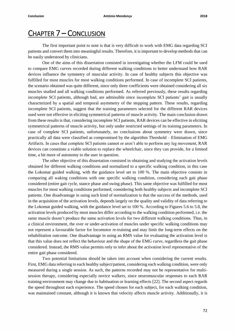
Conclusion António Mendonça 2018
72
CHAPTER 7 – CONCLUSION
The first important point to note is that is very difficult to work with EMG data regarding SCI
patients and convert them into meaningful results. Therefore, it is important to develop methods that can
be easily understood by clinicians.
One of the aims of this dissertation consisted in investigating whether the LFM could be used
to compare EMG curves recorded during different walking conditions to better understand how RAR
devices influence the symmetry of muscular activity. In case of healthy subjects this objective was
fulfilled for most muscles for most walking conditions performed. In case of incomplete SCI patients,
the scenario obtained was quite different, since only three coefficients were obtained considering all six
muscles studied and all walking conditions performed. As referred previously, these results regarding
incomplete SCI patients, although bad, are admissible since incomplete SCI patients’ gait is usually
characterized by a spatial and temporal asymmetry of the stepping pattern. These results, regarding
incomplete SCI patients, suggest that the training parameters selected for the different RAR devices
used were not effective in eliciting symmetrical patterns of muscle activity. The main conclusion drawn
from these results is that, considering incomplete SCI patients, RAR devices can be effective in eliciting
symmetrical patterns of muscle activity, but only under restricted settings of its training parameters. In
case of complete SCI patients, unfortunately, no conclusions about symmetry were drawn, since
practically all data were classified as compromised by the algorithm Threshold – Elimination of EMG
Artifacts. In cases that complete SCI patients cannot or aren’t able to perform any leg movement, RAR
devices can constitute a viable solution to replace the wheelchair, since they can provide, for a limited
time, a bit more of autonomy to the user in question.
The other objective of this dissertation consisted in obtaining and studying the activation levels
obtained for different walking conditions and normalized to a specific walking condition, in this case
the Lokomat guided walking, with the guidance level set to 100 %. The main objective consists in
comparing all waking conditions with one specific walking condition, considering each gait phase
considered (entire gait cycle, stance phase and swing phase). This same objective was fulfilled for most
muscles for most walking conditions performed, considering both healthy subjects and incomplete SCI
patients. One disadvantage in using such kind of normalization is that the success of the methods, used
in the acquisition of the activation levels, depends largely on the quality and validity of data referring to
the Lokomat guided walking, with the guidance level set to 100 %. According to Figures 5.6 to 5.8, the
activation levels produced by most muscles differ according to the walking condition performed, i.e. the
same muscle doesn’t produce the same activation levels for two different walking conditions. Thus, in
a clinical environment, the over or under-activation of muscles under specific walking conditions may
not represent a favourable factor for locomotor re-training and may limit the long-term effects on the
rehabilitation outcome. One disadvantage in using an RMS value for evaluating the activation level is
that this value does not reflect the behaviour and the shape of the EMG curve, regardless the gait phase
considered. Instead, the RMS value permits only to infer about the activation level representative of the
entire gait phase considered.
Two potential limitations should be taken into account when considering the current results.
First, EMG data referring to each healthy subject/patient, considering each walking condition, were only
measured during a single session. As such, the patterns recorded may not be representative for multi-
session therapy, considering especially novice walkers, since neuromuscular responses to each RAR
training environment may change due to habituation or learning effects [22]. The second aspect regards
the speed throughout each experience. The speed chosen for each subject, for each walking condition,
was maintained constant, although it is known that velocity affects muscle activity. Additionally, it is
Conclusion António Mendonça 2018
73
known that the mutual interactions between speed, level of guidance and BWS affect significantly the
muscle activity that each muscle display [23].
7.1 – Clinical Considerations
The physical support of limb movements to attain safe and successful stepping in the light of
impaired control, represents a general principle of locomotor training that is implemented in both
conventional physiotherapy and RAR. However, motor learning requires an active participation of the
patient and an inevitable consequence of providing physical support is that it decreases the necessity of
active contributions. Arguably, the potential of both Lokomat and Gait Trainer GT1 as gait-trainer
devices depend on the extent to which they encourage active contributions from the patient [22].
In order to stimulate the active participation of patients, RAR devices should operate in a way
that can selectively target specific impairments in locomotor task performance (e.g. impaired single
support phase), following the so-called assist-as-needed paradigm [12,20]. According to this paradigm,
patients are free to explore patterns, but they are assisted when failing to successfully complete the gait
cycle. In case of the Lokomat version used in the context of this dissertation, although the impedance
control that drives the exoskeleton allows the control of the overall guidance level, the timing of events
is fixed, and guidance is provided equally throughout the entire gait cycle [49,50]. However, the most
recent versions of the Lokomat exoskeleton have already implemented a “path control algorithm” that
produces a supportive force for the timing of events, which, in turn, can be set separately from the
guidance level [50,51]. This improvement allows more flexibly timed limb trajectories and intends to
enhance even more the purpose of the assist-as-needed paradigm.
7.2 – Future Perspectives
In short, the conjugational assessment of both activation levels and symmetry indexes can
constitute a useful tool to demarcate the benefits that RAR devices can bring to locomotor re-training.
Additionally, this evaluation performed over multiple sessions can bring even more benefits, since it
allows to determine which are the training parameters that best conform to a specific SCI patient, i.e.
which are the training parameters that can generate the best long-term results. In fact, the conjugational
assessment of both activation levels and symmetry indexes over multiple sessions can be used to
quantify and qualify the long-term learning effects produced during the locomotor training involving
RAR devices. Therefore, this conjugational assessment can constitute a great resource to construct
conventional, standardized and efficient protocols capable of optimizing the rehabilitation process.
Another challenge that still needs to be resolved is that practically all robotic systems are not
yet ready to be used in a domestic environment. This happens because the current systems are somehow
massive and those that are portable still do not present solutions regarding durable energy sources. In
case this scenario is altered, SCI patients will be allowed to perform the rehabilitation process directly
at home, without the extra effort required to go from home to the institution.

Bibliography António Mendonça 2018
74
BIBLIOGRAPHY
[1] R.R. Seeley, T.D. Stephens, P. Tate. “Anatomy and Physiology” (8th edition). McGraw Hill,
Chap. 9-14, pp. 374-506, 2008.
[2] Zannie’s Science Page (accessed at 15th of March 2017). Available at:
http://zanniedallara.weebly.com/bio-body-system.html
[3] Emaze’s Official Website, “Nervous System Images” (accessed at 28th of March 2017).
Available at: https://www.emaze.com/@AZLCCIFC/Nervous-system-images
[4] Chegg Study Webpage, “Seeley’s Principles of Anatomy and Physiology” (2nd edition),
Solutions for Chapter 12 Problem 4P (accessed at 20th of April 2017). Available at:
http://www.chegg.com/homework-help/use-figures-1112-123-124-125-129-1211-1212-answer-
questions-chapter-12-problem-4p-solution-9780077441487-exc
[5] MyHumanBody.ca Webpage (accessed at 29th of April 2017). Available at:
http://www.corpshumain.ca/en/Touche_en.php
[6] The Nervous System, published at 31st of January 2017 (accessed at 30th of May 2017).
Available at: https://mrdoddswebsite.weebly.com/uploads/5/4/8/2/5482575/the_nervous_system.pdf
[7] J.G. Webster. “Medical Instrumentation: Application and Design” (4th edition). John Wiley &
Sons, Inc, 2010.
[8] J. E. Lasfargues, D. Custis, F. Morrone, J. Carswell and T. Nguyen, “A model for estimating
spinal cord prevalence in the United States”, Paraplegia, vol. 33, pp. 62-68, 1995.
[9] Christopher & Dana REEVE Foundation, “What is a complete vs incomplete injury?” (accessed
at 12th May 2017). Available at: https://www.christopherreeve.org/living-with-paralysis/newly-
paralyzed/how-is-an-sci-defined-and-what-is-a-complete-vs-incomplete-injury
[10] D. P. Ferris, G. S. Sawicki, and A. R. Domingo, “Powered Lower Limb Orthoses for Gait
Rehabilitation”, Top Spinal Cord Injury Rehabilitation, vol. 11, no. 2, pp. 34-49, 2005.
[11] H. Schmidt, C. Werner, R. Bernhardt, S. Hesse, and J. Kruger, “Gait rehabilitation machines
based on programmable footplates,” Journal of NeuroEngineering and Rehabilitation, vol. 4, no. 2, pp.
1-3, 2007.
[12] I. Díaz, J. J. Gil, and E. Sánchez, “Lower-Limb Robotic Rehabilitation: Literature Review and
Challenges”, Journal of Robotics, vol. 2011, Article ID 759764, pp. 1-8, 5th September 2011.
[13] E. Mikolajewska, and D. Mikolajewski, “Exoskeletons in Neurological Diseases – Current and
Potential Future Applications, Adv Clin Exp Med, vol. 20, no. 2, pp. 227-233, 2011.
[14] A. M. Dollar and M. Cenciarini, “Biomechanical Considerations in the Design of Lower Limb
Exoskeletons”, IEEE International Conference on Rehabilitation Robotics, pp. 297-302, 2011.

Bibliography António Mendonça 2018
75
[15] BBC News, UK, Scotland, Edinburgh, Fife and East, “Scientists hope fish clues aid spinal cord
injury treatment”, published at 25th of July 2017 (accessed at 30th August 2017). Available at:
http://www.bbc.com/news/uk-scotland-edinburgh-east-fife-40715505
[16] A. M. Dollar and H. Herr, “Lower Extremity Exoskeletons and Active Orthoses: Challenges
and State-of-the-Art”, IEEE Transactions on Robotics, vol.24, no.1, pp. 144-56, February 2008.
[17] A. Bonnefoy-Mazure and S. Armand, “Normal Gait”, Orthopedic Management of Children with
Cerebral Palsy, Chap. 16, pp. 200-201, January 2015.
[18] ThoughtCo., “Anatomical Directional Terms and Body Planes” (accessed at 30th of March
2017). Available at: https://www.thoughtco.com/anatomical-directional-terms-and-body-planes-
373204
[19] FootEducation Webpage, “Biomechanics of Walking (Gait)” (accessed at 14th of April 2017).
Available at: https://www.footeducation.com/page/biomechanics-of-walking-gait
[20] K. H. Low, “Robot-Assisted Gait Rehabilitation: From Exoskeletons to Gait Systems”, Defense
Science Research Conference and Expo (DSR), pp. 1-9, 2011.
[21] M. Iosa, A. Cereatti, A. Merlo, I. Campanini, S. Paolucci and A. Cappozzo, “Assessment of
Waveform Similarity in Clinical Gait Data: The Linear Fit Method”, BioMed Research International,
vol. 2014, Article ID 214156, pp. 1-7, 2014.
[22] K. van Kammen, A. M. Boonstra, L. H. V. van der Woude, H. A. Reinders-Messelink, and R.
den Otter, “Differences in muscle activity and temporal step parameters between Lokomat guided
walking and treadmill walking in post-stroke hemiparetic patients and healthy walkers”, Journal of
NeuroEngineering and Rehabilitation, vol. 14 (1), no. 32, pp. 1-11, 2017.
[23] K. van Kammen, A. M. Boonstra, H. A. Reinders-Messelink, and R. den Otter, “The combined
effects of body weight support and gait speed on gait related muscle activity: a comparison between
walking in the Lokomat exoskeleton and regular treadmill walking”, Plos One 9(9): e107323. doi:
10.1371/journal.pone.0107323, vol. 9 (9), pp. 1-12, 16th September 2014.
[24] S. Hesse and D. Uhlenbrock, “A mechanized gait trainer for restoration of gait”, Journal of
Rehabilitation Research and Development, vol. 37, no. 6, pp. 701-708, November 2000.
[25] Reha-Stim Official Website, “Gait Trainer GT I” (accessed at 12th of June of 2017). Available
at: http://www.reha-stim.de/cms/index.php?id=76
[26] J. Mehrholz, B. Elsner, C. Werner, J. Kugler and M. Pohl, “Electromechanical-assisted training
for walking after stroke”, Cochrane Database of Systematic Reviews, issue 7, pp. 1-17, 10th May 2017.
[27] J. Mehrholz, J. Kugler and M. Pohl, “Locomotor training for walking after spinal cord injury”,
Cochrane Database of Systematic Reviews, issue 11, 14th November 2012.
[28] M. Wirz, D. H. Zemon, R. Rupp, A. Scheel, G. Colombo, V. Diezt and T. G. Hornby,
“Effectiveness of automated locomotor training in patients with chronic incomplete spinal cord injury:

Bibliography António Mendonça 2018
76
a multicenter trial.”, Archives of Physical Medicine and Rehabilitation, vol. 86 (4), pp. 672-680, April
2005.
[29] T. A. Wren, G. E. Gorton III, S. Ounpuu and C. A. Tucker, “Efficacy of clinical gait analysis.
A systematic review”, Gait & Posture, vol. 34 (2), pp. 149-153, June 2011.
[30] M. Halaki and K. Ginn, “Normalization of EMG Signals: To Normalize or Not to Normalize
and What to Normalize to?”, Computational Intelligence in Electromyography Analysis – A Perspective
on Current Applications and Future Challenges, Chap. 7, Dr. Ganesh R. Naik (Ed.), InTech, 17th
October 2012. Available from: https://www.intechopen.com/books/computational-intelligence-in-
electromyography-analysis-a-perspective-on-current-applications-and-future-
challenges/normalization-of-emg-signals-to-normalize-or-not-to-normalize-and-what-to-normalize-to-
[31] J. M. Hidler and A. E. Wall, “Alterations in muscle activation patterns during robotic-assisted
walking”, Clinical Biomechanics, vol. 20, issue 2, pp. 184-193, 2015.
[32] C. Werner, S. Von Frankenberg, T. Treig, M. Konrad and S. Hesse, “Treadmill training with
partial body weight support and an electromechanical gait trainer for restoration of gait in subacute
stroke patients: a randomized crossover study,” Stroke, vol. 33, no. 12, pp. 2895–2901, 2002.
[33] S. H. Peurala, O. Airaksinen, P. Huuskonen et al., “Effects of intensive therapy using gait trainer
or floor walking exercises early after stroke,” Journal of Rehabilitation Medicine, vol. 41, no. 3, pp.
166–173, 2009.
[34] G. Morone, S. Paolucci, A. Cherubini, D. De Angelis, V. Venturiero, P. Coiro and M. Iosa,
“Robot-assisted gait training for stroke patients: current state of the art and perspectives of robotics”,
Neuropsychiatric Disease and Treatment, vol. 13, pp. 1303-1311, 2017.
[35] “World Medic Association Declaration of Helsinki: ethical principles for medical research
involving human subjects”, JAMA, vol. 310, no. 20, pp. 2191-2194, 27th November 2013.
[36] H. J. Hermens, B. Freriks, G. Rau and C. Disselhorst-Klug, “The recommendations for sensor
and sensor placement procedures for surface electromyography.”, European recommendations for
surface electromyography, H. Hermens (Ed.), pp. 15-53, 1999.
[37] A. Lamontagne, C. L. Richards and F. Malouin, “Coactivation during gait as an adaptive
behavior after stroke”, Journal of Electromyography and Kinesiology, vol. 10 (6), pp. 407-415,
December 2000.
[38] P. Coenen, G. van Werven, M. P. van Nunen, J. H. van Dieën, K. H. Gerrits and T. W. Janssen,
“Robot-assisted walking vs overground walking in stroke patients: an evaluation of muscle activity”,
Journal of Rehabilitation Medicine, vol. 44 (4), pp. 331-337, April 2012.
[39] T. A. Schuler, R. Müller and H. J. van Hedel, “Leg surface electromyography patterns in
children with neuro-orthopedic disorders walking on a treadmill unassisted and assisted by a robot with
and without encouragement”, Journal of NeuroEngineering and Rehabilitation, vol. 10, no. 78, pp.1-
13, 2003.

Bibliography António Mendonça 2018
77
[40] TeachMeAnatomy.info, “Walking and Gaits” (accessed at 5th of August 2017). Available at:
http://teachmeanatomy.info/lower-limb/misc/walking-and-gaits/
[41] D. Thompson, “Muscle activity during the gait cycle” (accessed at 10th of August 2017).
Available at: http://ouhsc.edu/bserdac/dthompso/web/gait/kinetics/mmactsum.htm
[42] A. Singh, L. Tetreault, S. Kalsi-Ryan, A. Nouri and M. G. Fehlings, “Global prevalence and
incidence of traumatic spinal cord injury”, Clinical Epidemiology, vol. 6, pp. 309-331, 2014.
[43] S. Ferro, L. Cecconi, J. Bonavita, M. C. Pagliacci, A. Biggeri and M. Franceschini, “Incidence
of traumatic spinal cord injury in Italy during 2013-2014: a population-based study.”, Spinal Cord, 5th
September 2017.
[44] Encyclopedia Britannica, “Quadriceps femoris muscle” (accessed at 16th of August 2017).
Available at: https://www.britannica.com/science/quadriceps-femoris-muscle
[45] Wolfram MathWorld Official Website, “Root-Mean-Square” (accessed at 12th of September
2017). Available at: http://mathworld.wolfram.com/Root-Mean-Square.html
[46] SpinalCord.com, “Types of Spinal Cord Injuries” (accessed 10th of November 2017). Available
at: https://www.spinalcord.com/types-of-spinal-cord-injuries
[47] Shepherd Center, “Understanding Spinal Cord Injury” (accessed at 15th of November 2017).
Available at: http://www.spinalinjury101.org/details/asia-iscos
[48] ASIA (American Spinal Injury Association), “International Standards for Neurological
Classification of Spinal Cord Injury (ISNCSCI)”, provided by ISCOS (International Spinal Cord
Society) (accessed at 10th December 2017). Available at: http://asia-spinalinjury.org/wp-
content/uploads/2016/02/International_Stds_Diagram_Worksheet.pdf
[49] A. Duschau-Wicke, J. von Zitzewitz, A. Caprez, L. Lunenburger and R. Riener, “Path control:
a method for patient-cooperative robot-aided gait rehabilitation.”, IEEE Trans.Neural Syst. Rehab. Eng.,
vol. 38 (1), pp. 38-48, 2010.
[50] A. Duschau-Wicke, A. Caprez and R. Riener, “Patient-cooperative control increases active
participation of individuals with SCI during robot-aided gait training.”, Journal of NeuroEngineering
and Rehabilitation, vol. 7 (43), pp. 1-13, 2010.
[51] R. Riener, L. Lunenburger, I. Maier, G. Colombo and V. Dietz, “Locomotor Training in
Subjects with Sensori-Motor Deficits: An Overview of the Robotic Gait Orthosis Lokomat”, Journal of
Healthcare Engineering, vol. 1, no. 2, pp. 197-216, 2010.
[52] S. Freivogel, J. Mehrholz, T. Husak-Sotomayor, and D. Schmalohr, “Gait training with the
newly developed “LokoHelp”-system is feasible for non-ambulatory patients after stroke, spinal cord
and brain injury. A feasibility study,” Brain Injury, vol. 22 (7-8), pp. 625–632, 2008.
[53] G. R. West, “Powered gait orthosis and method of utilizing same,” Patent number 6 689 075,
2004.

Bibliography António Mendonça 2018
78
[54] M. Iosa, G. Morone, A. Fusco, M. Bragoni, P. Coiro, M. Multari, V. Venturiero, D. De Angelis,
L. Pratesi and S. Paolucci, “Seven Capital Devices for the Future of Stroke Rehabilitation”, Stroke
Research and Treatment, vol. 2012, Article ID 187965, pp. 1-9, 2012.
[55] W. H. Chang and Y. Kim, “Robot-assisted Therapy in Stroke Rehabilitation”, Journal of Stroke,
vol. 15, no. 3, pp. 174-181, September 2013.
[56] H. Y. Kim and J. S. H. You, “A Review of Robot-Assisted Gait Training in Stroke Patients”,
Brain Neurorehabilitation, vol. 10, no. 2, pp. 1-7, September 2017.
[57] J. Mehrholz and M. Pohl, “Electromechanical-Assisted Gait Training After Stroke: A
Systematic Review Comparing End-Effector and Exoskeleton Devices”, Journal of Rehabilitation
Medicine, vol. 44, number 3, pp. 193-199, March 2012.
[58] Health Information | A-Z of Medical Conditions | Patient, Dr. Mary Lowth, “Abnormal Gait”,
History and Examination, published at 12th of August 2014 (accessed at 4th of March 2018). Available
at: https://patient.info/doctor/abnormal-gait

Annexes António Mendonça 2018
79
ANNEXES
A) Healthy Subjects – Normalized EMG Profiles
Figure 5.14 – Normalized EMG profile for the healthy subject identified with the number 1 (see table 4.1). Time and
amplitude normalized EMG signals for each one of the 12 muscles considered (muscles’ names can be consulted in the
captions of Figures 5.1, 5.2 and 5.3). Each solid colored line represents the normalized average EMG signal of a specific
walking condition. The color scheme used for representing each walking condition is equal to the one that is used in
figure 5.4. Each dashed line represents the estimate of the stance phase’s duration of a specific walking condition and is
colored in accordance with the corresponding walking condition.
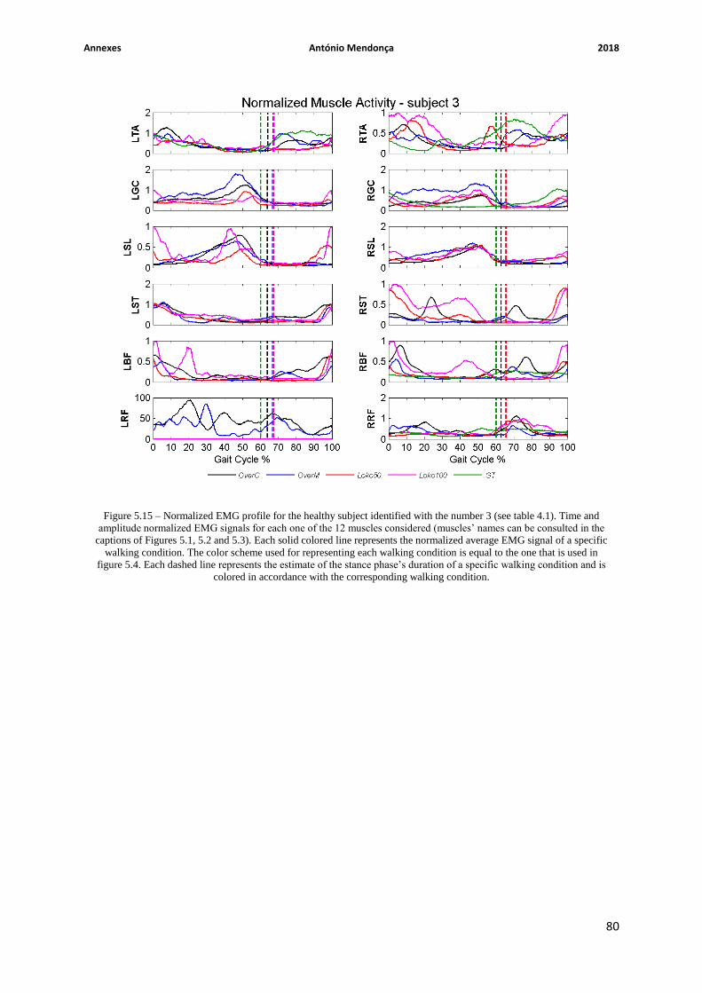
Annexes António Mendonça 2018
80
Figure 5.15 – Normalized EMG profile for the healthy subject identified with the number 3 (see table 4.1). Time and
amplitude normalized EMG signals for each one of the 12 muscles considered (muscles’ names can be consulted in the
captions of Figures 5.1, 5.2 and 5.3). Each solid colored line represents the normalized average EMG signal of a specific
walking condition. The color scheme used for representing each walking condition is equal to the one that is used in
figure 5.4. Each dashed line represents the estimate of the stance phase’s duration of a specific walking condition and is
colored in accordance with the corresponding walking condition.

Annexes António Mendonça 2018
81
Figure 5.16 – Normalized EMG profile for the healthy subject identified with the number 4 (see table 4.1). Time and
amplitude normalized EMG signals for each one of the 12 muscles considered (muscles’ names can be consulted in the
captions of Figures 5.1, 5.2 and 5.3). Each solid colored line represents the normalized average EMG signal of a specific
walking condition. The color scheme used for representing each walking condition is equal to the one that is used in
figure 5.4. Each dashed line represents the estimate of the stance phase’s duration of a specific walking condition and is
colored in accordance with the corresponding walking condition.

Annexes António Mendonça 2018
82
Figure 5.17 – Normalized EMG profile for the healthy subject identified with the number 5 (see table 4.1). Time and
amplitude normalized EMG signals for each one of the 12 muscles considered (muscles’ names can be consulted in the
captions of Figures 5.1, 5.2 and 5.3). Each solid colored line represents the normalized average EMG signal of a specific
walking condition. The color scheme used for representing each walking condition is equal to the one that is used in
figure 5.4. Each dashed line represents the estimate of the stance phase’s duration of a specific walking condition and is
colored in accordance with the corresponding walking condition.

Annexes António Mendonça 2018
83
Figure 5.18 – Normalized EMG profile for the healthy subject identified with the number 6 (see table 4.1). Time and
amplitude normalized EMG signals for each one of the 12 muscles considered (muscles’ names can be consulted in the
captions of Figures 5.1, 5.2 and 5.3). Each solid colored line represents the normalized average EMG signal of a specific
walking condition. The color scheme used for representing each walking condition is equal to the one that is used in
figure 5.4. Each dashed line represents the estimate of the stance phase’s duration of a specific walking condition and is
colored in accordance with the corresponding walking condition.

Annexes António Mendonça 2018
84
Figure 5.19 – Normalized EMG profile for the healthy subject identified with the number 7 (see table 4.1). Time and
amplitude normalized EMG signals for each one of the 12 muscles considered (muscles’ names can be consulted in the
captions of Figures 5.1, 5.2 and 5.3). Each solid colored line represents the normalized average EMG signal of a specific
walking condition. The color scheme used for representing each walking condition is equal to the one that is used in
figure 5.4. Each dashed line represents the estimate of the stance phase’s duration of a specific walking condition and is
colored in accordance with the corresponding walking condition.

Annexes António Mendonça 2018
85
Figure 5.20 – Normalized EMG profile for the healthy subject identified with the number 8 (see table 4.1). Time and
amplitude normalized EMG signals for each one of the 12 muscles considered (muscles’ names can be consulted in the
captions of Figures 5.1, 5.2 and 5.3). Each solid colored line represents the normalized average EMG signal of a specific
walking condition. The color scheme used for representing each walking condition is equal to the one that is used in
figure 5.4. Each dashed line represents the estimate of the stance phase’s duration of a specific walking condition and is
colored in accordance with the corresponding walking condition.

Annexes António Mendonça 2018
86
Figure 5.21 – Normalized EMG profile for the healthy subject identified with the number 9 (see table 4.1). Time and
amplitude normalized EMG signals for each one of the 12 muscles considered (muscles’ names can be consulted in the
captions of Figures 5.1, 5.2 and 5.3). Each solid colored line represents the normalized average EMG signal of a specific
walking condition. The color scheme used for representing each walking condition is equal to the one that is used in
figure 5.4. Each dashed line represents the estimate of the stance phase’s duration of a specific walking condition and is
colored in accordance with the corresponding walking condition.
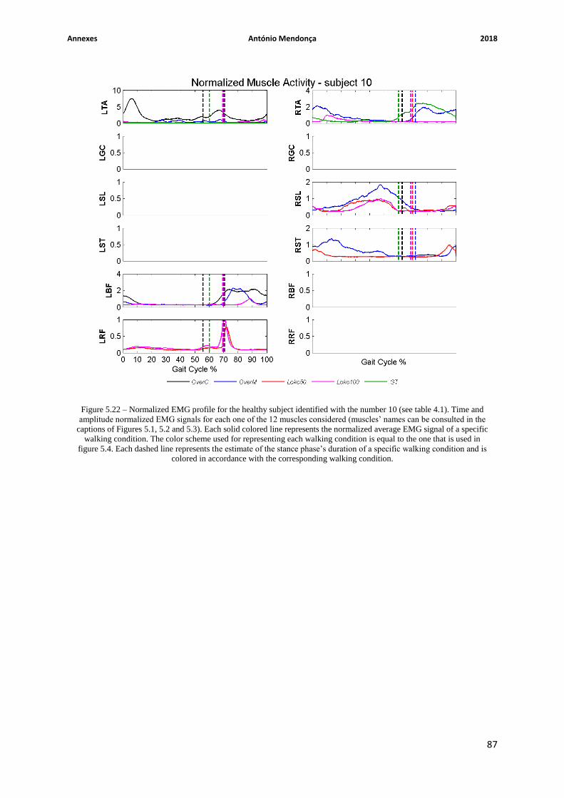
Annexes António Mendonça 2018
87
Figure 5.22 – Normalized EMG profile for the healthy subject identified with the number 10 (see table 4.1). Time and
amplitude normalized EMG signals for each one of the 12 muscles considered (muscles’ names can be consulted in the
captions of Figures 5.1, 5.2 and 5.3). Each solid colored line represents the normalized average EMG signal of a specific
walking condition. The color scheme used for representing each walking condition is equal to the one that is used in
figure 5.4. Each dashed line represents the estimate of the stance phase’s duration of a specific walking condition and is
colored in accordance with the corresponding walking condition.

Annexes António Mendonça 2018
88
B) Incomplete SCI Patients – Normalized EMG Profiles
Figure 5.23 – Normalized EMG profile for the incomplete SCI patient identified with the number 1 (see table 4.2). Time
and amplitude normalized EMG signals for each one of the 12 muscles considered (muscles’ names can be consulted in
the captions of Figures 5.1, 5.2 and 5.3). Each solid colored line represents the normalized average EMG signal of a
specific walking condition. The color scheme used for representing each walking condition is equal to the one that is
used in figure 5.5. Each dashed line represents the estimate of the stance phase’s duration of a specific walking condition
and is colored in accordance with the corresponding walking condition.

Annexes António Mendonça 2018
89
Figure 5.24 – Normalized EMG profile for the incomplete SCI patient identified with the number 2 (see table 4.2). Time
and amplitude normalized EMG signals for each one of the 12 muscles (muscles’ names can be consulted in the captions
of Figures 5.1, 5.2 and 5.3). Each solid colored line represents the normalized average EMG signal of a specific walking
condition. The color scheme used for representing each walking condition is equal to the one that is used in figure 5.5.
Each dashed line represents the estimate of the stance phase’s duration of a specific walking condition and is colored in
accordance with the corresponding walking condition.

Annexes António Mendonça 2018
90
Figure 5.25 – Normalized EMG profile for the incomplete SCI patient identified with the number 3 (see table 4.2). Time
and amplitude normalized EMG signals for each one of the 12 muscles (muscles’ names can be consulted in the captions
of Figures 5.1, 5.2 and 5.3). Each solid colored line represents the normalized average EMG signal of a specific walking
condition. The color scheme used for representing each walking condition is equal to the one that is used in figure 5.5.
Each dashed line represents the estimate of the stance phase’s duration of a specific walking condition and is colored in
accordance with the corresponding walking condition.

Annexes António Mendonça 2018
91
Figure 5.26 – Normalized EMG profile for the incomplete SCI patient identified with the number 4 (see table 4.2). Time
and amplitude normalized EMG signals for each one of the 12 muscles considered (muscles’ names can be consulted in
the captions of Figures 5.1, 5.2 and 5.3). Each solid colored line represents the normalized average EMG signal of a
specific walking condition. The color scheme used for representing each walking condition is equal to the one that is
used in figure 5.5. Each dashed line represents the estimate of the stance phase’s duration of a specific walking condition
and is colored in accordance with the corresponding walking condition.
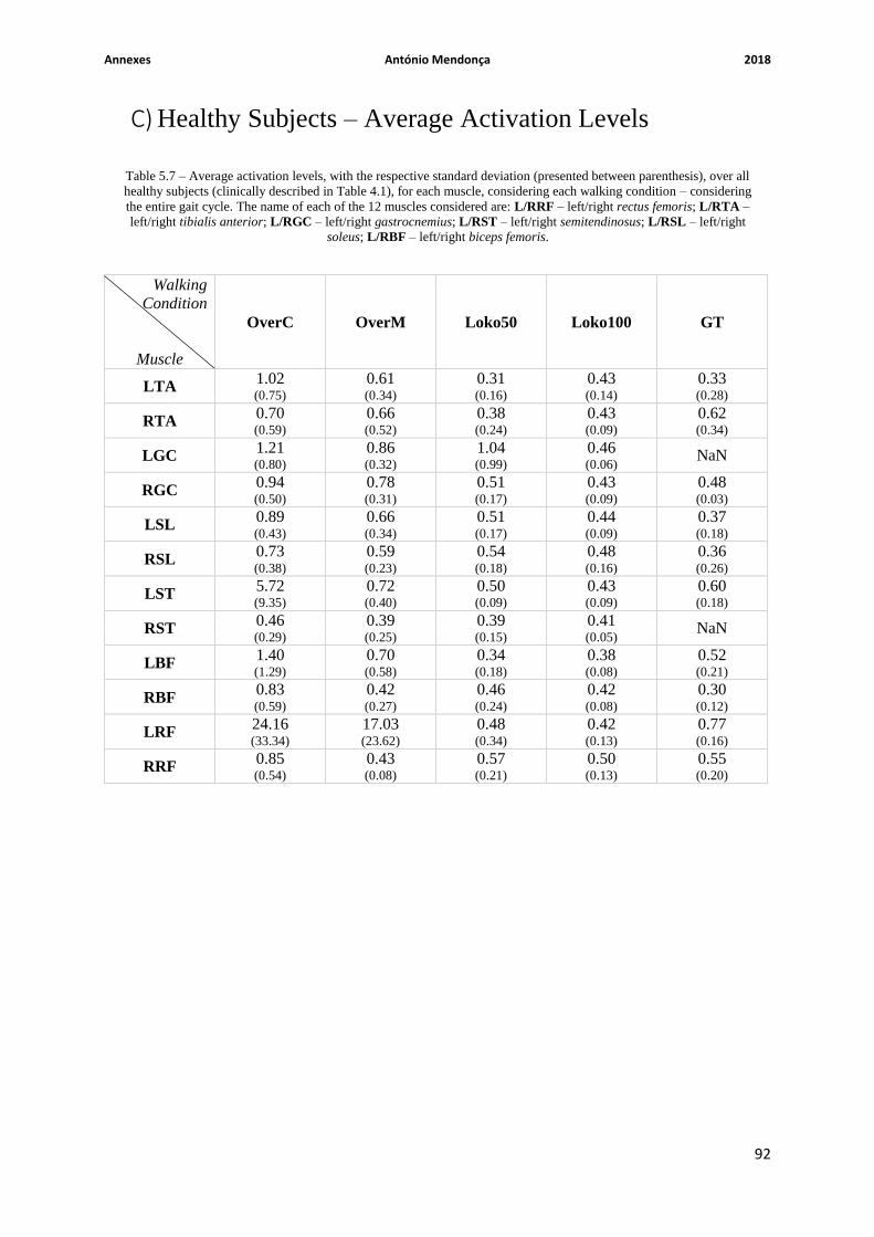
Annexes António Mendonça 2018
92
C) Healthy Subjects – Average Activation Levels
Walking
Condition
Muscle
OverC OverM Loko50 Loko100 GT
LTA 1.02 (0.75)
0.61 (0.34)
0.31 (0.16)
0.43 (0.14)
0.33 (0.28)
RTA 0.70 (0.59)
0.66 (0.52)
0.38 (0.24)
0.43 (0.09)
0.62 (0.34)
LGC 1.21 (0.80)
0.86 (0.32)
1.04 (0.99)
0.46 (0.06)
NaN
RGC 0.94 (0.50)
0.78 (0.31)
0.51 (0.17)
0.43 (0.09)
0.48 (0.03)
LSL 0.89 (0.43)
0.66 (0.34)
0.51 (0.17)
0.44 (0.09)
0.37 (0.18)
RSL 0.73 (0.38)
0.59 (0.23)
0.54 (0.18)
0.48 (0.16)
0.36 (0.26)
LST 5.72 (9.35)
0.72 (0.40)
0.50 (0.09)
0.43 (0.09)
0.60 (0.18)
RST 0.46 (0.29)
0.39 (0.25)
0.39 (0.15)
0.41 (0.05)
NaN
LBF 1.40 (1.29)
0.70 (0.58)
0.34 (0.18)
0.38 (0.08)
0.52 (0.21)
RBF 0.83 (0.59)
0.42 (0.27)
0.46 (0.24)
0.42 (0.08)
0.30 (0.12)
LRF 24.16 (33.34)
17.03 (23.62)
0.48 (0.34)
0.42 (0.13)
0.77
(0.16)
RRF 0.85 (0.54)
0.43 (0.08)
0.57 (0.21)
0.50 (0.13)
0.55 (0.20)
Table 5.7 – Average activation levels, with the respective standard deviation (presented between parenthesis), over all
healthy subjects (clinically described in Table 4.1), for each muscle, considering each walking condition – considering
the entire gait cycle. The name of each of the 12 muscles considered are: L/RRF – left/right rectus femoris; L/RTA –
left/right tibialis anterior; L/RGC – left/right gastrocnemius; L/RST – left/right semitendinosus; L/RSL – left/right
soleus; L/RBF – left/right biceps femoris.

Annexes António Mendonça 2018
93
Walking
Condition
Muscle
OverC OverM Loko50 Loko100 GT
LTA 1.00 (0.82)
0.61 (0.34)
0.35 (0.19)
0.46 (0.16)
0.20 (0.18)
RTA 0.66 (0.55)
0.59 (0.40)
0.42 (0.27)
0.48 (0.11)
0.22 (0.13)
LGC 1.50 (1.04)
1.02 (0.39)
1.20 (1.19)
0.48 (0.03)
NaN
RGC 1.16 (0.62)
0.94 (0.37)
0.58 (0.23)
0.48 (0.12)
0.48 (0.20)
LSL 1.12 (0.55)
0.80 (0.41)
0.59 (0.21)
0.50 (0.09)
0.44 (0.24)
RSL 0.92 (0.52)
0.71 (0.28)
0.60 (0.18)
0.53 (0.15)
0.42 (0.34)
LST 6.04
(10.24)
0.75 (0.41)
0.48 (0.14)
0.48 (0.12)
0.57 (0.17)
RST 0.33 (0.24)
0.42 (0.28)
0.37 (0.20)
0.40 (0.14)
NaN
LBF 1.22 (1.33)
0.48 (0.31)
0.34 (0.24)
0.37 (0.14)
0.52 (0.21)
RBF 0.66 (0.47)
0.40 (0.31)
0.46 (0.32)
0.42 (0.12)
0.30 (0.16)
LRF 26.51 (36.53)
18.40 (25.60)
0.44 (0.30)
0.36 (0.15)
0.50
(0.00)
RRF 0.89 (0.66)
0.42 (0.05)
0.50 (0.25)
0.39 (0.17)
0.42 (0.10)
Table 5.8 – Average activation levels, with the respective standard deviation (presented between parenthesis), over all
healthy subjects (clinically described in Table 4.1), for each muscle, considering each walking condition – considering
only the stance phase. The name of each of the 12 muscles considered are: L/RRF – left/right rectus femoris; L/RTA –
left/right tibialis anterior; L/RGC – left/right gastrocnemius; L/RST – left/right semitendinosus; L/RSL – left/right
soleus; L/RBF – left/right biceps femoris.

Annexes António Mendonça 2018
94
Walking
Condition
Muscle
OverC OverM Loko50 Loko100 GT
LTA 0.93 (0.79)
0.54 (0.41)
0.18 (0.13)
0.30 (0.23)
0.38 (0.38)
RTA 0.69 (0.73)
0.75 (0.77)
0.26 (0.21)
0.24 (0.18)
0.84 (0.66)
LGC 0.29 (0.18)
0.23 (0.15)
0.34 (0.25)
0.31 (0.20)
NaN
RGC 0.23 (0.14)
0.21 (0.10)
0.24 (0.14)
0.27 (0.17)
0.28 (0.30)
LSL 0.16 (0.09)
0.11 (0.06)
0.21 (0.14)
0.21 (0.15)
0.15 (0.12)
RSL 0.17 (0.14)
0.16 (0.10)
0.25 (0.13)
0.26 (0.15)
0.16 (0.13)
LST 4.62 (7.77)
0.58 (0.45)
0.42 (0.25)
0.32 (0.18)
0.51 (0.35)
RST 0.51 (0.42)
0.27 (0.21)
0.36 (0.21)
0.34 (0.21)
NaN
LBF 1.36 (1.36)
0.84 (1.03)
0.25 (0.18)
0.30 (0.20)
0.37 (0.30)
RBF 0.89 (0.80)
0.35 (0.28)
0.32 (0.22)
0.34 (0.22)
0.20 (0.15)
LRF 12.91 (22.04)
9.24 (15.67)
0.36 (0.47)
0.38 (0.31)
0.70
(0.64)
RRF 0.50 (0.48)
0.33 (0.25)
0.51 (0.36)
0.52 (0.31)
0.56 (0.41)
Table 5.9 – Average activation levels, with the respective standard deviation (presented between parenthesis), over all
healthy subjects (clinically described in Table 4.1), for each muscle, considering each walking condition – considering
only the swing phase. The name of each of the 12 muscles considered are: L/RRF – left/right rectus femoris; L/RTA –
left/right tibialis anterior; L/RGC – left/right gastrocnemius; L/RST – left/right semitendinosus; L/RSL – left/right
soleus; L/RBF – left/right biceps femoris.

Annexes António Mendonça 2018
95
Whole Gait Cycle Stance Phase Swing Phase
Walking
Condition
(Muscle)
Healthy
Walker
OverC (LST)
OverC (LRF)
OverM (LRF)
OverC (LST)
OverC (LRF)
OverM (LRF)
OverC (LST)
OverC (LRF)
OverM (LRF)
1 0.56 NaN NaN 0.48 NaN NaN 0.68 NaN NaN
2 0.53 NaN NaN 0.54 NaN NaN 0.48 NaN NaN
3 0.52 47.74 33.73 0.50 52.34 36.50 0.56 38.34 27.34
4 1.71 NaN NaN 1.62 NaN NaN 1.85 NaN NaN
5 NaN NaN NaN NaN NaN NaN NaN NaN NaN
6 11.50 0.59 0.33 11.32 0.68 0.30 11.80 0.36 0.39
7 NaN NaN NaN NaN NaN NaN NaN NaN NaN
8 0.38 NaN NaN 0.37 NaN NaN 0.40 NaN NaN
9 24.85 NaN NaN 27.44 NaN NaN 21.22 NaN NaN
10 NaN NaN NaN NaN NaN NaN NaN NaN NaN
Average
RMS
value (standard
deviation)
5.72 (9.35)
24.16 (33.34)
17.03 (23.62)
6.04 (10.24)
26.51 (36.53)
18.40 (25.60)
4.62 (7.77)
12.91 (22.04)
9.24 (15.67)
Table 5.10 – Activation levels of each healthy subject (clinically described in Table 4.1) for the left semitendinosus
(LST) while performing the self-paced over-ground walking (OverC), and the left rectus femoris (LRF) while
performing the self-paced over-ground walking and the over-ground walking guided by a metronome (OverM),
considering each gait phase – the whole gait cycle, the stance phase and the swing phase. The muscles previously
referred are indicated between parenthesis.
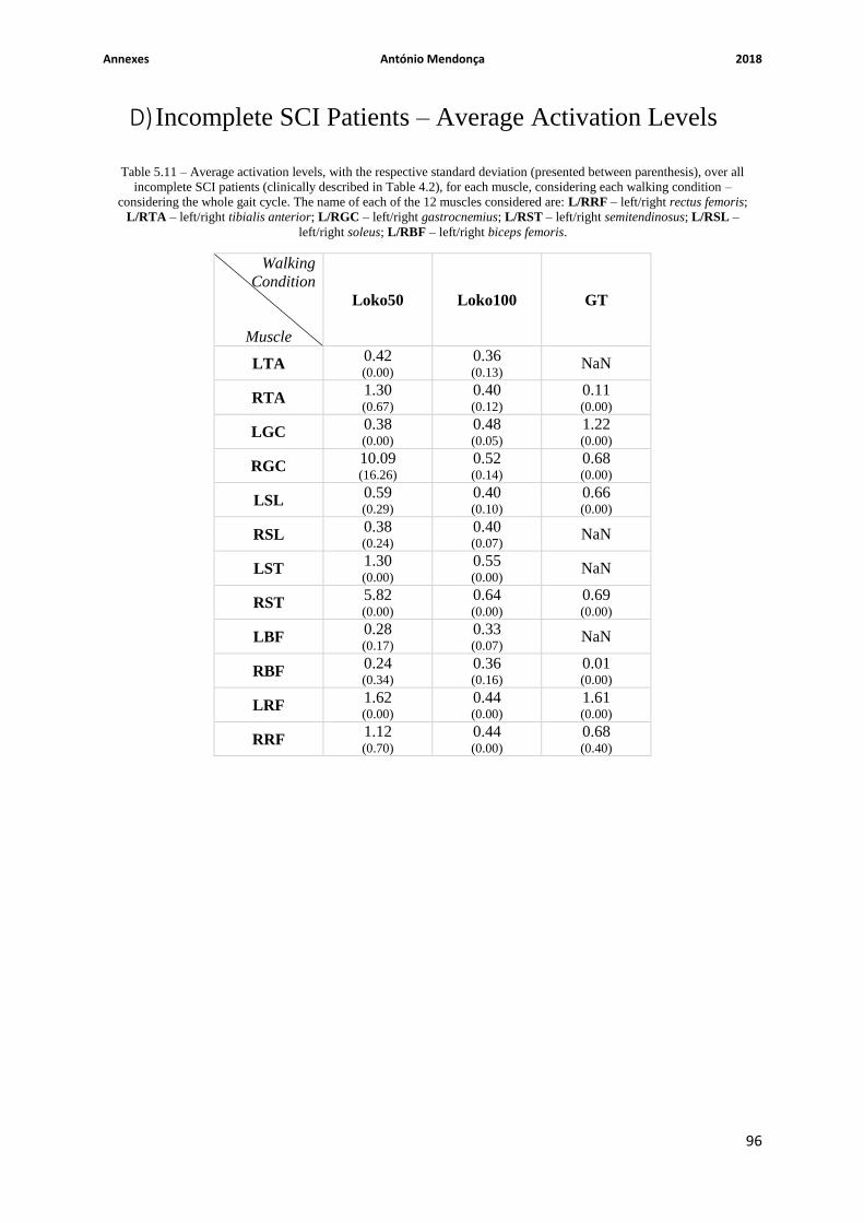
Annexes António Mendonça 2018
96
D) Incomplete SCI Patients – Average Activation Levels
Walking
Condition
Muscle
Loko50 Loko100 GT
LTA 0.42 (0.00)
0.36 (0.13)
NaN
RTA 1.30 (0.67)
0.40 (0.12)
0.11 (0.00)
LGC 0.38 (0.00)
0.48 (0.05)
1.22 (0.00)
RGC 10.09 (16.26)
0.52 (0.14)
0.68 (0.00)
LSL 0.59 (0.29)
0.40 (0.10)
0.66 (0.00)
RSL 0.38 (0.24)
0.40 (0.07)
NaN
LST 1.30 (0.00)
0.55 (0.00)
NaN
RST 5.82 (0.00)
0.64 (0.00)
0.69 (0.00)
LBF 0.28 (0.17)
0.33 (0.07)
NaN
RBF 0.24 (0.34)
0.36 (0.16)
0.01 (0.00)
LRF 1.62 (0.00)
0.44 (0.00)
1.61
(0.00)
RRF 1.12 (0.70)
0.44 (0.00)
0.68 (0.40)
Table 5.11 – Average activation levels, with the respective standard deviation (presented between parenthesis), over all
incomplete SCI patients (clinically described in Table 4.2), for each muscle, considering each walking condition –
considering the whole gait cycle. The name of each of the 12 muscles considered are: L/RRF – left/right rectus femoris;
L/RTA – left/right tibialis anterior; L/RGC – left/right gastrocnemius; L/RST – left/right semitendinosus; L/RSL –
left/right soleus; L/RBF – left/right biceps femoris.

Annexes António Mendonça 2018
97
Walking
Condition
Muscle
Loko50 Loko100 GT
LTA 0.45 (0.00)
0.40 (0.14)
NaN
RTA 1.34 (0.62)
0.44 (0.10)
0.12 (0.00)
LGC 0.42 (0.00)
0.50 (0.06)
0.12 (0.00)
RGC 8.43
(13.28)
0.51 (0.14)
0.72 (0.00)
LSL 0.67 (0.36)
0.44 (0.13)
0.69 (0.00)
RSL 0.40 (0.24)
0.39 (0.01)
NaN
LST 1.36 (0.00)
0.58 (0.00)
NaN
RST 4.07 (0.00)
0.69 (0.00)
0.66 (0.00)
LBF 0.21 (0.11)
0.28 (0.11)
NaN
RBF 0.11 (0.15)
0.33 (0.28)
0.01 (0.00)
LRF 1.92 (0.00)
0.48 (0.00)
1.94
(0.00)
RRF 1.26 (0.80)
0.47 (0.06)
0.54 (0.53)
Table 5.12 – Average activation levels, with the respective standard deviation (presented between parenthesis), over all
incomplete SCI patients (clinically described in Table 4.2), for each muscle, considering each walking condition –
considering only the stance phase. The name of each of the 12 muscles considered are: L/RRF – left/right rectus
femoris; L/RTA – left/right tibialis anterior; L/RGC – left/right gastrocnemius; L/RST – left/right semitendinosus;
L/RSL – left/right soleus; L/RBF – left/right biceps femoris.

Annexes António Mendonça 2018
98
Walking
Condition
Muscle
Loko50 Loko100 GT
LTA 0.34 (0.00)
0.25 (0.11)
NaN
RTA 1.22 (0.78)
0.26 (0.23)
0.10 (0.00)
LGC 0.22 (0.00)
0.42 (0.04)
1.17 (0.00)
RGC 12.69 (21.06)
0.52 (0.16)
0.62 (0.00)
LSL 0.35 (0.05)
0.28 (0.01)
0.62 (0.00)
RSL 0.33 (0.24)
0.39 (0.20)
NaN
LST 1.17 (0.00)
0.46 (0.00)
NaN
RST 8.52 (0.00)
0.50 (0.00)
0.74 (0.00)
LBF 0.36 (0.29)
0.34 (0.24)
NaN
RBF 0.40 (0.56)
0.34 (0.08)
0.01 (0.00)
LRF 0.58 (0.00)
0.33 (0.00)
0.94
(0.00)
RRF 0.70 (0.39)
0.35 (0.16)
0.75 (0.46)
Table 5.13 – Average activation levels, with the respective standard deviation (presented between parenthesis), over all
incomplete SCI patients (clinically described in Table 4.2), for each muscle, considering each walking condition –
considering only the swing phase. The name of each of the 12 muscles considered are: L/RRF – left/right rectus femoris;
L/RTA – left/right tibialis anterior; L/RGC – left/right gastrocnemius; L/RST – left/right semitendinosus; L/RSL –
left/right soleus; L/RBF – left/right biceps femoris.

Annexes António Mendonça 2018
99
Whole Gait Cycle Stance Phase Swing Phase
Walking
Condition
(Muscle)
Patient
Loko50 (RGC)
Loko50 (RST)
Loko50 (RGC)
Loko50 (RST)
Loko50 (RGC)
Loko50 (RST)
1 NaN NaN NaN NaN NaN NaN
2 NaN NaN NaN NaN NaN NaN
3 28.87 NaN 23.76 NaN 37.02 NaN
4 0.51 NaN 0.52 NaN 0.49 NaN
5 0.90 5.82 1.00 4.07 0.58 8.52
Average
RMS
value (standard
deviation)
10.09 (16.26)
5.82 (0.00)
8.43 (13.28)
4.07 (0.00)
12.69 (21.06)
8.52 (0.00)
Table 5.14 – Activation levels of each incomplete SCI patient (clinically described in Table 4.2) for the right
gastrocnemius (RGC) and the right semitendinosus (RST) while performing the Lokomat guided walking, with the
guidance level set to 50 % (Loko50), considering each gait phase – the whole gait cycle, the stance phase and the swing
phase. The muscles previously referred are indicated between parenthesis.
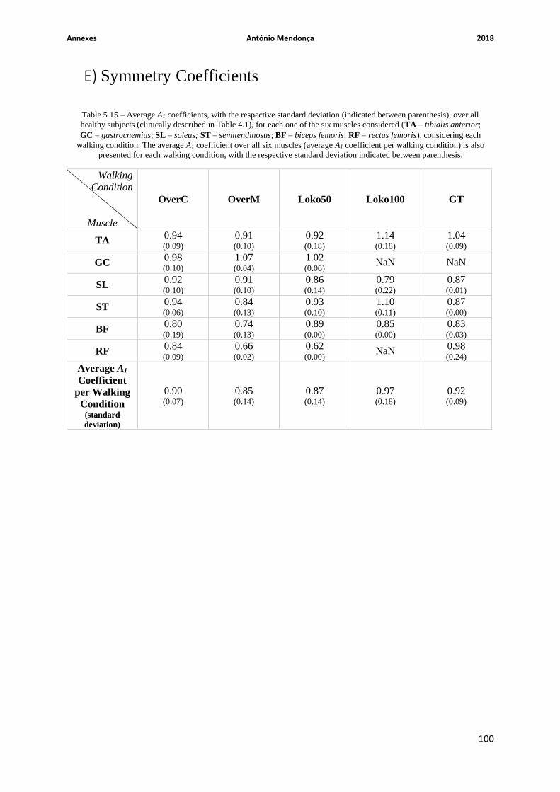
Annexes António Mendonça 2018
100
E) Symmetry Coefficients
Walking
Condition
Muscle
OverC OverM Loko50 Loko100 GT
TA 0.94 (0.09)
0.91 (0.10)
0.92 (0.18)
1.14 (0.18)
1.04 (0.09)
GC 0.98 (0.10)
1.07 (0.04)
1.02 (0.06)
NaN NaN
SL 0.92 (0.10)
0.91 (0.10)
0.86 (0.14)
0.79 (0.22)
0.87 (0.01)
ST 0.94 (0.06)
0.84 (0.13)
0.93 (0.10)
1.10 (0.11)
0.87 (0.00)
BF 0.80 (0.19)
0.74 (0.13)
0.89 (0.00)
0.85 (0.00)
0.83 (0.03)
RF 0.84 (0.09)
0.66 (0.02)
0.62 (0.00)
NaN 0.98 (0.24)
Average A1
Coefficient
per Walking
Condition (standard
deviation)
0.90 (0.07)
0.85 (0.14)
0.87 (0.14)
0.97 (0.18)
0.92 (0.09)
Table 5.15 – Average A1 coefficients, with the respective standard deviation (indicated between parenthesis), over all
healthy subjects (clinically described in Table 4.1), for each one of the six muscles considered (TA – tibialis anterior;
GC – gastrocnemius; SL – soleus; ST – semitendinosus; BF – biceps femoris; RF – rectus femoris), considering each
walking condition. The average A1 coefficient over all six muscles (average A1 coefficient per walking condition) is also
presented for each walking condition, with the respective standard deviation indicated between parenthesis.
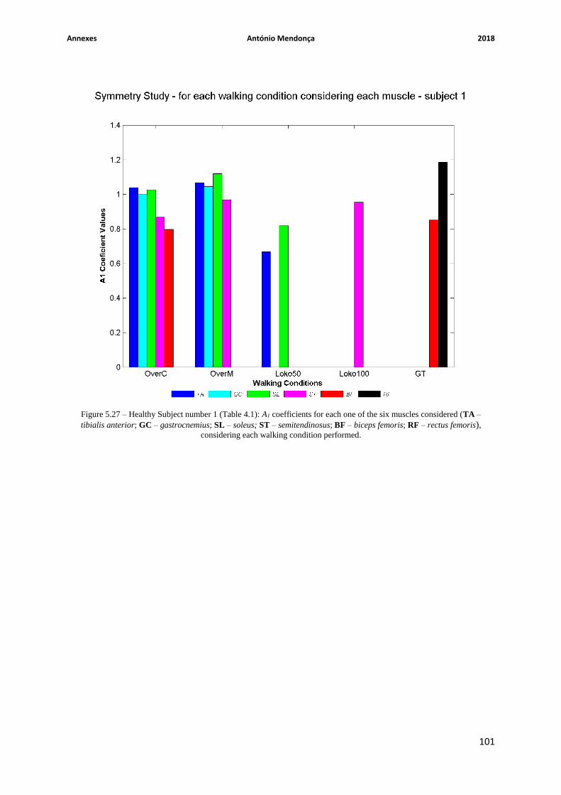
Annexes António Mendonça 2018
101
Figure 5.27 – Healthy Subject number 1 (Table 4.1): A1 coefficients for each one of the six muscles considered (TA –
tibialis anterior; GC – gastrocnemius; SL – soleus; ST – semitendinosus; BF – biceps femoris; RF – rectus femoris), considering each walking condition performed.

Annexes António Mendonça 2018
102
Figure 5.28 – Healthy Subject number 2 (Table 4.1): A1 coefficients for each one of the six muscles considered (TA –
tibialis anterior; GC – gastrocnemius; SL – soleus; ST – semitendinosus; BF – biceps femoris; RF – rectus femoris), considering each walking condition performed.

Annexes António Mendonça 2018
103
Figure 5.29 – Healthy Subject number 3 (Table 4.1): A1 coefficients for each one of the six muscles considered (TA –
tibialis anterior; GC – gastrocnemius; SL – soleus; ST – semitendinosus; BF – biceps femoris; RF – rectus femoris), considering each walking condition performed.
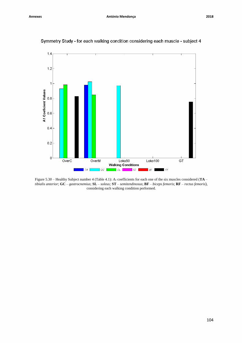
Annexes António Mendonça 2018
104
Figure 5.30 – Healthy Subject number 4 (Table 4.1): A1 coefficients for each one of the six muscles considered (TA –
tibialis anterior; GC – gastrocnemius; SL – soleus; ST – semitendinosus; BF – biceps femoris; RF – rectus femoris), considering each walking condition performed.

Annexes António Mendonça 2018
105
Figure 5.31 – Healthy Subject number 5 (Table 4.1): A1 coefficients for each one of the six muscles considered (TA –
tibialis anterior; GC – gastrocnemius; SL – soleus; ST – semitendinosus; BF – biceps femoris; RF – rectus femoris), considering each walking condition performed.

Annexes António Mendonça 2018
106
Figure 5.32 – Healthy Subject number 6 (Table 4.1): A1 coefficients for each one of the six muscles considered (TA –
tibialis anterior; GC – gastrocnemius; SL – soleus; ST – semitendinosus; BF – biceps femoris; RF – rectus femoris), considering each walking condition performed.

Annexes António Mendonça 2018
107
Figure 5.33 – Healthy Subject number 7 (Table 4.1): A1 coefficients for each one of the six muscles considered (TA –
tibialis anterior; GC – gastrocnemius; SL – soleus; ST – semitendinosus; BF – biceps femoris; RF – rectus femoris), considering each walking condition performed.

Annexes António Mendonça 2018
108
Figure 5.34 – Healthy Subject number 8 (Table 4.1): A1 coefficients for each one of the six muscles considered (TA –
tibialis anterior; GC – gastrocnemius; SL – soleus; ST – semitendinosus; BF – biceps femoris; RF – rectus femoris), considering each walking condition performed.

Annexes António Mendonça 2018
109
Figure 5.35 – Healthy Subject number 9 (Table 4.1): A1 coefficients for each one of the six muscles considered (TA –
tibialis anterior; GC – gastrocnemius; SL – soleus; ST – semitendinosus; BF – biceps femoris; RF – rectus femoris), considering each walking condition performed.

Annexes António Mendonça 2018
110
Figure 5.36 – Healthy Subject number 10 (Table 4.1): A1 coefficients for each one of the six muscles considered (TA –
tibialis anterior; GC – gastrocnemius; SL – soleus; ST – semitendinosus; BF – biceps femoris; RF – rectus femoris), considering each walking condition performed.

Annexes António Mendonça 2018
111
Walking
Condition
Muscle
Loko50 Loko100 GT
TA NaN NaN NaN
GC NaN NaN NaN
SL NaN NaN NaN
ST NaN NaN 0.84 (0.00)
BF NaN NaN NaN
RF 0.78 (0.00)
NaN 0.89 (0.00)
Average A1
Coefficient
per Walking
Condition (standard
deviation)
0.78 (0.00)
NaN 0.86 (0.04)
Table 5.16 – Average A1 coefficients, with the respective standard deviation (indicated between parenthesis), over all
incomplete SCI patients (clinically described in Table 4.2), for each one of the six muscles considered (TA – tibialis
anterior; GC – gastrocnemius; SL – soleus; ST – semitendinosus; BF – biceps femoris; RF – rectus femoris), considering each walking condition. The average A1 coefficient over all six muscles (average A1 coefficient per walking
condition) is also presented for each walking condition, with the respective standard deviation indicated between
parenthesis.

Annexes António Mendonça 2018
112
Figure 5.37 – Incomplete SCI patient number 1 (Table 4.2): A1 coefficients for each one of the six muscles considered
(TA – tibialis anterior; GC – gastrocnemius; SL – soleus; ST – semitendinosus; BF – biceps femoris; RF – rectus
femoris), considering each walking condition performed.

Annexes António Mendonça 2018
113
Figure 5.38 – Incomplete SCI patient number 2 (Table 4.2): A1 coefficients for each one of the six muscles considered
(TA – tibialis anterior; GC – gastrocnemius; SL – soleus; ST – semitendinosus; BF – biceps femoris; RF – rectus
femoris), considering each walking condition performed.
Annexes António Mendonça 2018
114
Figure 5.39 – Incomplete SCI patient number 3 (Table 4.2): A1 coefficients for each one of the six muscles considered
(TA – tibialis anterior; GC – gastrocnemius; SL – soleus; ST – semitendinosus; BF – biceps femoris; RF – rectus
femoris), considering each walking condition performed.
Annexes António Mendonça 2018
115
Figure 5.40 – Incomplete SCI patient number 4 (Table 4.2): A1 coefficients for each one of the six muscles considered
(TA – tibialis anterior; GC – gastrocnemius; SL – soleus; ST – semitendinosus; BF – biceps femoris; RF – rectus
femoris), considering each walking condition performed.

Annexes António Mendonça 2018
116
Figure 5.41 – Incomplete SCI patient number 5 (Table 4.2): A1 coefficients for each one of the six muscles considered
(TA – tibialis anterior; GC – gastrocnemius; SL – soleus; ST – semitendinosus; BF – biceps femoris; RF – rectus
femoris), considering each walking condition performed.