Nine linear motion plants for teaching fundamental and ...

Nine linear motion plants for teaching fundamental and advanced controls concepts

STUDENT WORKBOOKLinear Flexible Joint Experiment for LabVIEW Users

Standardized for ABET* Evaluation Criteria

Developed by:Jacob Apkarian, Ph.D., Quanser

Hervé Lacheray, M.A.SC., QuanserPeter Martin, M.A.SC., Quanser

Quanser educational solutions are powered by:

Courseware complies with:

CAPTIVATE. MOTIVATE. GRADUATE. * ABET Inc., is the recognized accreditor for college and university programs in applied science, computing, engineering, and technology. ABET has provided leadership and quality assurance in higher education for over 75 years.

c⃝ 2012 Quanser Inc., All rights reserved.

Quanser Inc.119 Spy CourtMarkham, OntarioL3R [email protected]: 1-905-940-3575Fax: 1-905-940-3576

Printed in Markham, Ontario.

For more information on the solutions Quanser Inc. offers, please visit the web site at:http://www.quanser.com

This document and the software described in it are provided subject to a license agreement. Neither the software nor this document may beused or copied except as specified under the terms of that license agreement. All rights are reserved and no part may be reproduced, stored ina retrieval system or transmitted in any form or by any means, electronic, mechanical, photocopying, recording, or otherwise, without the priorwritten permission of Quanser Inc.

LFJC-E Workbook - Student Version 2

http://www.quanser.com

CONTENTS1 Introduction 4

2 Modeling 52.1 Background 52.2 Pre-Lab Questions 102.3 In-Lab Exercises 11

3 Position Control 173.1 Specifications 173.2 Background 173.3 Pre-Lab Questions 193.4 In-Lab Exercises 20

4 System Requirements 244.1 Overview of Files 244.2 Software Setup 25

5 Lab Report 275.1 Template for Content 275.2 Tips for Report Format 28

LFJC-E Workbook - Student Version v 1.0

1 INTRODUCTIONThe objective of this laboratory is to develop a feedback system to track the spring-driven cart to a desired position asquickly as possible while minimizing the overshoot and residual vibration. A full-state-feedback controller is designedusing the Linear Quadratic Regulator (LQR) methodology.

Topics Covered

• Developing of a mathematical model of the linear flexible joint system using Lagrangian mechanics.

• Obtaining the linear state-space representation of the open-loop system

• Designing a state-feedback controller using the LQR algorithm.

• Simulating the closed-loop system to ensure that the specifications are met

• Implementing the controller on the LFJC-E plant and evaluating its performance

Prerequisites

In order to successfully carry out this laboratory, the user should be familiar with the following:

• The required software and hardware outlined in Section 4.

• State-space modeling fundamentals.

• Some knowledge of state-feedback.

• Basics of LabVIEWTM .

• Laboratory described in the LabVIEW Integration [2] in order to be familiar using LabVIEWTM with the IP02Base Unit.


2 MODELING

2.1 Background

2.1.1 Model Convention

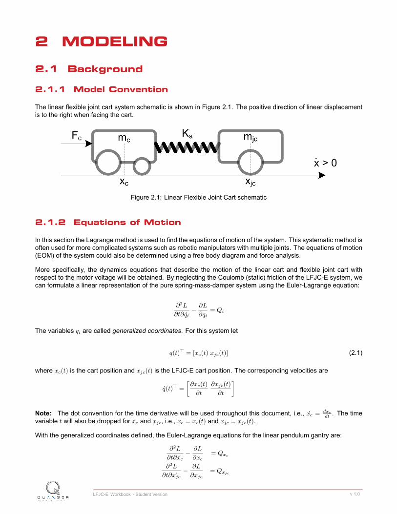
The linear flexible joint cart system schematic is shown in Figure 2.1. The positive direction of linear displacementis to the right when facing the cart.

Figure 2.1: Linear Flexible Joint Cart schematic

2.1.2 Equations of Motion

In this section the Lagrange method is used to find the equations of motion of the system. This systematic method isoften used for more complicated systems such as robotic manipulators with multiple joints. The equations of motion(EOM) of the system could also be determined using a free body diagram and force analysis.

More specifically, the dynamics equations that describe the motion of the linear cart and flexible joint cart withrespect to the motor voltage will be obtained. By neglecting the Coulomb (static) friction of the LFJC-E system, wecan formulate a linear representation of the pure spring-mass-damper system using the Euler-Lagrange equation:

∂2L

∂t∂qi− ∂L

∂qi= Qi

The variables qi are called generalized coordinates. For this system let

q(t)⊤ = [xc(t) xjc(t)] (2.1)

where xc(t) is the cart position and xjc(t) is the LFJC-E cart position. The corresponding velocities are

q(t)⊤ =

[∂xc(t)

∂t

∂xjc(t)

∂t

]

Note: The dot convention for the time derivative will be used throughout this document, i.e., xc = dxc

dt . The timevariable t will also be dropped for xc and xjc, i.e., xc = xc(t) and xjc = xjc(t).

With the generalized coordinates defined, the Euler-Lagrange equations for the linear pendulum gantry are:

∂2L

∂t∂xc− ∂L

∂xc= Qxc

∂2L

∂t∂ ˙xjc− ∂L

∂xjc= Qxjc


The Lagrangian of the system, L, is described:L = T − V

where T is the total kinetic energy of the system and V is the total potential energy of the system. Therefore, theLagrangian represents the difference between the kinetic and potential energy of the system.

The potential energy of a system is fundamentally a measure of the energy that a system has due to some kind ofwork that was performed to move it from a lower energy configuration. In the case of the LFJC-E since the verticalmotions of the carts are fixed, the system's total potential energy is due to the elastic potential energy of the linearspring. Therefore, the total potential energy of system is:

VT =1

2Ks(xjc − xc)

2 (2.2)

where Ks is the joint spring constant.

The total kinetic energy of the system is the sum of the translational and rotational kinetic energies arising from themotion of the IP02 cart, and the translational kinetic energy of the LFJC-E cart. The translational kinetic energy ofthe IP02 cart, Tct, can be expressed as:

Tct =1

2mcxc

2

and the rotational energy due to the DC motor, Tcr, is:

Tcr =1

2

ηgJmK2g xc

2

r2mp

where the corresponding IP02 parameters are defined in the IP02 User Manual [1]. Finally, the translational kineticenergy of the LFJC-E is:

Tjct =1

2mjc ˙xjc

2

If we combine the kinetic energy equations together, the resultant total kinetic energy of the system is:

TT =1

2Jeqxc

2 +1

2mjcx

2jc (2.3)

where

Jeq = M +ηgK

2gJm

r2mp

The generalized forces, Qxc and Qxjc , are used to describe the non-conservative forces applied to a system withrespect to the generalized coordinates. The generalized forces acting on the linear carts are:

Qxc = Fc −Beqxc (2.4)

and acting on the pendulum isQxjc = −Beqjc xjc. (2.5)

where Beq and Beqjc are the equivalent viscous damping of the IP02 and LFJC-E carts respectively.

Note: The nonlinear Coulomb friction applied to the linear carts have been neglected in the dynamic model.

By substituting the total kinetic and potential energy of the system shown in Equation 2.2 and Equation 2.3, and thegeneralized forces into the Euler-Lagrange formulation, the equations of motion are:

Jeqxc +Ksxc −Ksx2 = Fc −Beqxc (2.6)


andmjcxjc −Ksxc +Ksxjc = −Beqjc xjc. (2.7)

Solving for the acceleration terms in the equations of motion yields:

xc =1

Jeq

(−Ksxc +Ksxjc −Beqxc + Fc

)(2.8)

and

xjc =1

mjc

(Ksxc −Ksxjc −Beqjc xjc

). (2.9)

The linear force applied to the cart, Fc, is generated by the servo motor and described by the equation:

Fc =ηgKgKt

Rmrmp

(−KgKmxc

rmp+ ηmVm

)(2.10)

where the servo motor parameters are defined in the IP02 User Manual [1].

The equations of motion for the IP02 and LFJC-E derived in Equation 2.8 and Equation 2.9 match the typical formof an EOM for a single body:

Jx+ bx+ g(x) = F1 (2.11)

where x is a linear position, J is the moment of inertia, b is the damping, g(x) is the gravitational function, and F1 isthe applied force (scalar value).

For a generalized coordinate vector q, this can be generalized into the matrix form

D(q)q + C(q, q)q + g(q) = F (2.12)

where D is the inertial matrix, C is the damping matrix, g(q) is the gravitational vector, and F is the applied forcevector.

The equations of motion given in 2.6 and 2.7 can be placed into this matrix format.

2.1.3 State-Space Model

The linear state-space equations arex = Ax+Bu (2.13)

andy = Cx+Du

where x is the state, u is the control input, A, B, C, and D are state-space matrices. For the linear pendulum gantrysystem, the state and output are defined

x⊤ = [xc xjc xc xjc] (2.14)

andy⊤ = [xc xjc]. (2.15)

In the output equation, only the position of the IP02 and LFJC-E carts are being measured. Based on this, the Cand D matrices in the output equation are

C =

[1 0 0 00 1 0 0

](2.16)


andD =

[00

]. (2.17)

The velocities of the carts can be computed in the digital controller by taking the derivative and filtering the resultthough a high-pass filter.

2.1.4 Free-Oscillation of a Second Order System

Figure 2.2: Free Oscillation Response

Finding the Natural Frequency

The period of the oscillations in a system response can be found using the equation

Tosc =tn+1 − t1

n(2.18)

where tn is the time of the nth oscillation, t1 is the time of the first peak, and n is the number of oscillations considered.From this, the damped natural frequency (in radians per second) is

ωd =2π

Tosc(2.19)

and the undamped natural frequency isωn =

ωd√1− ζ2

. (2.20)

Finding the Damping Ratio

The damping ratio of a second-order system can be found from its response. For a typical second-order under-damped system, the subsidence ratio (i.e., decrement ratio) is defined as

δ =1

nln

O1

On+1(2.21)


where O1 is the peak of the first oscillation and On is the peak of the nth oscillation. Note that O1 > On, as this is adecaying response.

The damping ratio is definedζ =

1√1 + 2π

δ

2(2.22)


2.2 Pre-Lab Questions

1. Find the linear state-space model of the flexible joint cart system.

2. Consider the linear spring-damper-mass portion of the system having parameters Ks, Beqjc , and mjc respec-tively. If the displacement of the mass center of gravity is xjc, determine the ordinary differential equation(ODE) that describes the free-oscillatory motion of the mass. Hint: Refer to the generalized second ordersingle body EOM shown in Equation 2.11.

3. Taking the Laplace transform of the ODE describing the free motion of the mass found in Question 2, expressthe coefficients of the ODE in terms of the generic damping and natural frequency parameters, ζ and ωn, foundin the second-order characteristic equation:

s2 + 2ζωns+ ω2n (2.23)

Note: For an underdamped system where ζ < 1, the roots of the characteristic equation are the complexconjugate roots:

s1 = −ζωn + jωn

√1− ζ2

ands2 = −ζωn − jωn

√1− ζ2


2.3 In-Lab Exercises

The goal of this laboratory is to explore the state-space model of the linear flexible joint cart. You will begin bydetermining the damping and spring constant of your particular LFJC-E. You will then conduct an experiment tovalidate the model by comparing the response of the model to the response of the actual system.

2.3.1 Impulse Response Test

Experimental Setup

The LFJC Model Parameters VI shown in Figure 2.3 is used to measure the impulse response of the LFJC-E loadcart.

Figure 2.3: LabVIEW VI used to measure LFJC-E impulse response

Note: Before you can conduct these experiments, you need to make sure that the lab files are configured accordingto your IP02 and LFJC-E setup. If they have not been configured already, then go to Section 4.2 to configure thelab files before you begin.

1. Open the LabVIEW project called Linear Flexible Joint Cart.lvproj, shown in Figure 4.1, in Section 4.2.

2. Open the LFJC Model Parameters.vi shown in Figure 2.3.

3. If you haven't already, set the HIL Initialize vi to match your DAQ board as described in Section 4.2.

4. Clamp the IP02 cart to the track end-plate so that it cannot move.

5. With the IP02 cart immobile, you should be able to fully compress the linear spring by pushing on the LFJC-Eload cart. When the cart is released, the spring restoring force will apply an impulse force and initiate freeoscillations of the LFJC-E spring-damper-mass system.

6. Run the VI. Release the load cart and observe the oscillations on the LFJC-E Cart Position chart. When theoscillations have decayed significantly, click on the Stop button.


7. Your response should resemble the scope shown in Figure 2.4. Plot the response of the load cart and attachit to your report.

Figure 2.4: LFJC-E load cart impulse response

8. Using the response from Question 7 and the subsidence ratio Equation 2.21, calculate the experimental damp-ing ratio, ζ. You can use the Graph Palette to zoom in on the response.

9. Using the measured damping ratio, we can now calculate the experimental natural frequency of the system.Using the response from Question 7 and the period of the oscillations expressed in Equation 2.18, calculatethe experimental natural frequency, ωn.

10. Using the measured values of ζ and ωn, and the relationship you derived in Section 2.2, determine the exactvalues of the equivalent spring stiffness, Ks, and equivalent damping coefficient, Beqjc , that correspond toyour particular LFJC-E system. How do your values compare to the specification values of Ks = 142 N/m andBeqjc = 2.2 N-s/m, given in the LFJC-E User Manual [3]?Note: The mass of the LFJC-E load cart with the spring assembly is 0.293 kg, and each additional weight is0.125 kg. Therefore, the total mass of the LFJC-E load cart with two weights, mjc, is 0.543 kg.

2.3.2 Model Analysis

The LFJC Model Design VI shown in Figure 2.5 is used to create the state-space model of the linear flexible jointcart system. Once the model has been constructed using the state matrices that were developed in Section 2.2, youcan export the state-space model for use in other VIs.


1. Ensure that you have configured the lab files for your IP02 and LFJC-E setup. If they have not been configuredalready, then go to Section 4.2 to configure the lab files before you begin.


3. Open the SPG Model Design.vi shown in Figure 2.5.

4. Open the MathScript window under Tools | MathScript Window.

5. Open the setup lfjc model student script. Nearthe bottom of the script, you should find the following code:


Figure 2.5: VI used to confirm system model

A = eye(4,4);B = [0;0;1;0];C = eye(2,4);D = zeros(2,1);

%Actuator DynamicsA(3,3) = A(3,3) - B(3)*eta_g*Kg^2*eta_m*Kt*Km/r_mp^2/Rm;A(4,3) = A(4,3) - B(4)*eta_g*Kg^2*eta_m*Kt*Km/r_mp^2/Rm;B = eta_g*Kg*eta_m*Kt/r_mp/Rm*B;

The representative C andD matrices have already been included. You need to enter the state-space matricesA and B that you found in Section 2.2. The actuator dynamics have been added to convert your state-spacematrices to be in terms of voltage. Recall that the input of the state-space model you found in Section 2.2 is theforce acting on the IP02 cart. However, we do not control force directly - we control the servo input voltage. Theabove code uses the voltage-torque relationship given in Equation 2.10 in Section 2.1.2 to transform torque tovoltage.Note: The model parameters are denoted as Jeq, M jc, Beq jc, Ks, and Beq.

6. Run the setup lfjc model student script to load the state-space matrices. Show the numerical matrices thatare displayed in the Output Window.

7. Copy the resultant state-space matrices into the A and B fields in the LFJC Model Design VI. Run the modelto verify that the parameters were loaded properly.

8. Using the VI, record the open-loop poles of the system.

9. Enter a title for the state-space model in the Model Name field and press Save to export a copy of the modelinto the Model Files folder.

10. Update the values of the equivalent spring stiffness, Ks, and equivalent LFJC-E damping, Beqjc, with theexperimental values you found in Section 2.3.1. The values can be entered in the following script location:


% ##### USER-DEFINED MODEL PARAMETERS #####% Specify perticular equivalent spring stiffness, Ks, and equivalent% damping, Beq_jc, parameters:

%Ks = 0;%Beq_jc = 0;

11. Copy the updated state-space matrices into the A and B fields in the LFJC Model Design VI. Run the modelto verify that the parameters were loaded properly.

12. Enter a title for the alternative state-space model in the Model Name field and press Save to export a copy ofthe model into the Model Files folder.

Before ending this lab... To do the pre-lab questions in Section 3.3, you need the A and B matrices (numericalrepresentation) and the open-loop poles. Make sure you record these.


2.3.3 Model Validation

Experimental Setup

The LFJC Modeling VI shown in Figure 2.6 is used to confirm that the actual system hardware matches the state-space model derived in Section 2.1.3. This VI applies a voltage to the DC motor, and outputs the IP02 and LFJC-Ecart positions, as well as the spring deflection.

Figure 2.6: LabVIEW VI used to confirm system model



2. Open LFJC Modeling.vi shown in Figure 2.6.


4. Before starting the VI, load the state-space model you developed in Section 2.3.2 by double-clicking on theState-Space block on the block diagram, and clicking on ''Load Model''.

5. Ensure that the LFJC-E is in the middle of the track, and that the motor and encoder cables are able to movefreely.

6. Run the VI. The IP02 cart, and LFJC-E load cart should begin moving back and forth along the track, and thegraphs should resemble Figure 2.7. The blue trace is the simulated position of the cart, and the red trace isthe corresponding measured position.


Figure 2.7: IP02 open-loop step response

7. Load the state-space model that was generated using the experimental values for the equivalent damping andstiffenss parameters.

8. Re-run themodel and observe any changes in the response. Does the updated simulation match themeasuredresponse better than the default? Why might this be the case?

9. Create a figure that compares the simulated and experimental response of the cart positions and spring de-flection. Comment on why there may be discrepancies in the response of the updated model and the actualsystem.


3 POSITION CONTROL

3.1 Specifications

The response of the linear flexible joint cart should satisfy the following requirements:

• Percent Overshoot: PO ≤ 10 %

• Maximum settling time (5 %): ts ≤ 0.6 s

• Steady-state error: ess = 0.The control effort should be minimized as much as possible within the specified hard limit.

Note: The previous specifications are given in response to a ±20 mm square wave cart position setpoint.

3.2 Background

3.2.1 Linear Quadratic Regular (LQR)

If (A,B) are controllable, then the Linear Quadratic Regular optimization method can be used to find a feedbackcontrol gain. Given the plant model in Equation 2.13, the LQR algorithm finds the control input u that minimizes thecost function

J =

∫ ∞

0

x(t)′Qx(t) + u(t)′Ru(t) dt, (3.1)

where Q and R are the weighting matrices. The weighting matrices affect how LQR minimizes the function and are,essentially, tuning variables.

Given the control law u = −Kx, the state-space becomes

x = Ax+B(−Kx)

= (A−BK)x

Designing a controller with the Linear Quadratic Regular (LQR) technique is an iterative process. In software, youhave to select the Q and R matrices, generate the gain K using the LQR algorithm, and then simulate the systemor implement the control to access the control performance. The relationship between changing Q and R and theclosed-loop response is not evident. However, we can gain insight into how changing the different elements in Qand R will effect the response. We will only be changing the diagonal elements in Q, thus let

Q =

q1 0 0 00 q2 0 00 0 q3 00 0 0 q4

. (3.2)

Since we are dealing with a single-input system, R is a scalar value. Using the Q and R defined, the cost functiongiven in Equation 3.1 becomes:

J =

∫ ∞

0

q1x21 + q2x

22 + q3x

23 + q4x

24 +Ru2 dt. (3.3)


3.2.2 Feedback Control

The feedback control loop that controls the position of the mass cart is illustrated in Figure 3.1. The reference stateis defined

xd = [xjcd 0 0 0]

where xjcd is the desired LFJC-E load cart position. The controller is

u = K(xjcd − x). (3.4)

Note that when xjcd = 0 then u = −Kx, which is the control used in the LQR algorithm.

Figure 3.1: State-feedback control loop


3.3 Pre-Lab Questions

1. Based on the location of the open-loop poles determined in Section 2.1.1, what can you infer about the stabilityand dynamic behaviour of the open-loop system?

2. For the feedback control u = −Kx, the Linear-Quadratic Regular algorithm finds a gain K that minimizes thecost function J . Matrix Q sets the weight on the states and determines how u will minimize J (and hence howit generates gain K). From the relationship between the cost function and Q and R parameters expressed inEquation 3.3, explain how increasing the diagonal elements, qi, effects the generated gain K = [k1 k2 k3 k4].

3. Explain the effect of increasing R has on the generated gain, K.

4. Based on your results in Question 1 and Question 2, predict which elements of the Q matrix will require thelargest weight in order to achieve the system specifications outlined in Section 3.1.


3.4 In-Lab Exercises

The goal of this laboratory is to design a state-feedback controller for the linear flexible joint cart system using theLinear-Quadratic-Regulator (LQR) algorithm. The controller is then implemented on the system, and an experimentis conducted to access the performance of the controller.

3.4.1 Control Simulation

Experiment Setup

The LFJC Control Design VI shown in Figure 3.2 is used to simulate the closed-loop response of the linear flexiblejoint cart using the state-feedback control described in Section 3.2.2 with the control gain K. The response of thesystem is simulated to verify that the specifications are met, and the motor is not saturated.

Figure 3.2: VI used to simulate the state-feedback control

Note: Before you can conduct this experiment, you need to make sure that the lab files are configured accordingto your system setup. If they have not been configured already, go to Section 4.2 to configure the lab files first.


2. Open the LFJC Control Design.vi shown in Figure 3.2.



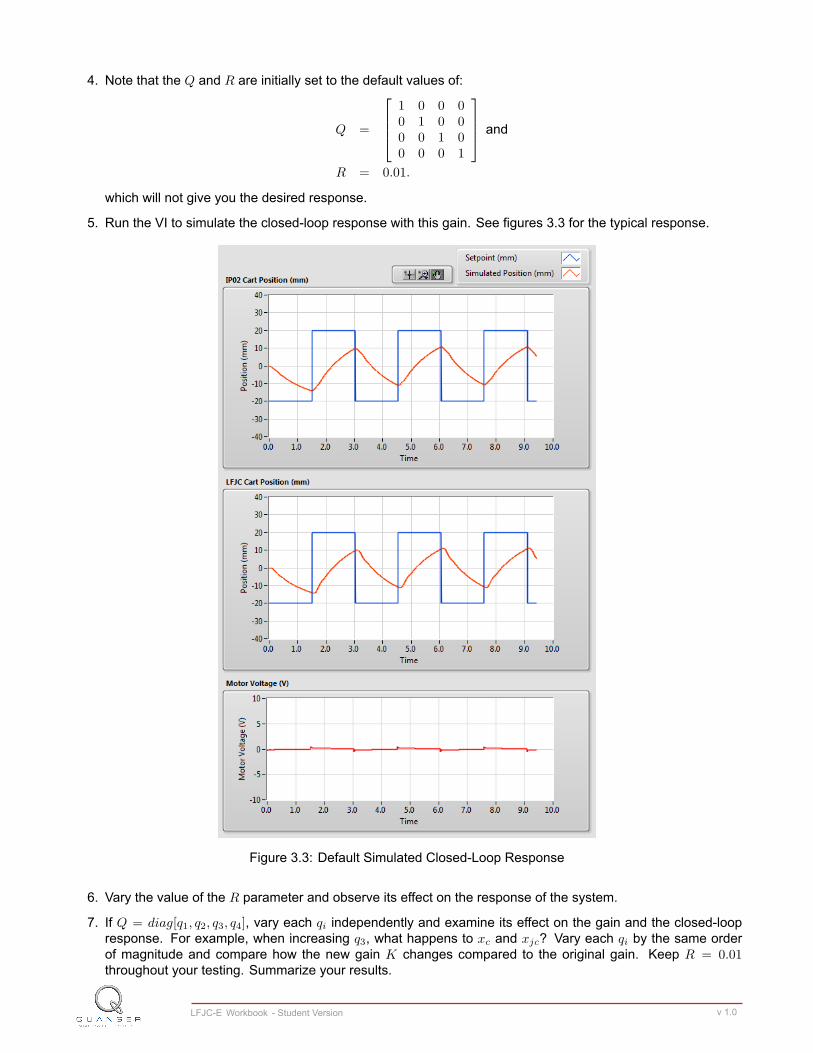
4. Note that the Q and R are initially set to the default values of:

Q =

1 0 0 00 1 0 00 0 1 00 0 0 1

and

R = 0.01.

which will not give you the desired response.

5. Run the VI to simulate the closed-loop response with this gain. See figures 3.3 for the typical response.

Figure 3.3: Default Simulated Closed-Loop Response

6. Vary the value of the R parameter and observe its effect on the response of the system.

7. If Q = diag[q1, q2, q3, q4], vary each qi independently and examine its effect on the gain and the closed-loopresponse. For example, when increasing q3, what happens to xc and xjc? Vary each qi by the same orderof magnitude and compare how the new gain K changes compared to the original gain. Keep R = 0.01throughout your testing. Summarize your results.


Note: Recall your analysis in pre-lab Question 2 where the effect of adjusting Q on the generated K wasassessed generally by inspecting the cost function equation. You may find some discrepancies in this exerciseand the pre-lab questions.

8. Find a Q and R that will satisfy the specifications given in Section 3.1. When doing this, try to maintain alow-amplitude smooth control signal within ±10 V. This control will later be implemented on actual hardware.Enter the weighting matrices, Q and R, used and the resulting gain, K.Note: Recall that the most important design objective for the controller is to maintain the pendulum in thebalanced inverted position.

9. Record the responses from the Cart Position (mm), LFJC Cart Position (mm), and Motor Voltage (V) scopes.

10. Measure the settling time and overshoot of the simulated LFJC-E load cart position response. Does the re-sponse satisfy the specifications given in Section 3.1?

3.4.2 Control Implementation

In this section, the LQR based state-feedback controller that was designed and simulated in the previous sectionsis run on the actual linear flexible joint cart.

Experiment Setup

The LFJC Position Control VI shown in Figure 3.4 is used to implement the LFJC-E controller with the controlgains that were developed using the LQR algorithm. The response of the system is measured to verify that thespecifications are met.

Figure 3.4: VI used to implement the LFJC position controller


Note: Before you can conduct these experiments, you need to make sure that the lab files are configured accordingto your IP02 and LFJC-E. If they have not been configured already, then go to Section 4.2 to configure the lab filesbefore you begin.


2. Open the LFJC Position Control.vi shown in Figure 3.4.


4. Ensure that the LFJC-E system is in the centre of the track. Run the VI.

5. The response should resemble the simulation. Once you have obtained a suitable response, click on the STOPbutton to stop the controller. Use the graphs to plot the IP02 cart, LFJC-E cart, and motor voltage responsesin a figure.

6. Measure the settling time, overshoot, and steady-state error of the LFJC-E load cart position. Are the specifi-cations given in Section 3.1 satisfied?

7. How could you alter the controller to compensate for the steady-state error?

3.4.3 Partial-State Feedback


2. Open the LFJC Position Control.vi shown in Figure 3.4.


4. Enter the control gain that you found in Section 3.4.1 into the Feedback Gain field.

5. Set the State-Feedback toggle to the Partial-State Feedback (downward) position.

6. Ensure that the LFJC-E system is in the centre of the track. Run the VI.

7. Stop the controller once you have obtained a representative response.

8. Create a figure representing the IP02 cart and LFJC-E cart position response.

9. Examine the difference between the partial-state feedback (PSF) response and the full-state feedback (FSF)response. Explain the behaviour of PSF control by examining the block diagram.

10. Turn off the power to the amplifier if no more experiments will be performed in this session.


4 SYSTEM REQUIREMENTSRequired Hardware

• IP02 and LFJC-E as described the IP02 User Manual [1], and the LFJC-E User Manual [3].

• Power Amplifier (e.g., Quanser VoltPAQ-X1)

• Data Acquisition Device (e.g., Quanser Q1-cRIO, Q2-USB, or NI DAQ with the Quanser-NI Terminal board)

Required Software

Make sure LabVIEWTM is installed with the following required add-ons:

1. LabVIEWTM

2. NI-DAQmx

3. NI LabVIEWTM Control Design and Simulation Module

4. NI LabVIEWTM MathScript RT Module

5. Quanser Rapid Control Prototyping Toolkitr

Note: Make sure the Quanser Rapid Control Prototyping (RCP) Toolkit is installed after LabVIEW. See the RCPToolkit Quick Start Guide for more information.

4.1 Overview of Files

File Name DescriptionLinear Flexible Joint Cart Workbook (Student).pdf This laboratory guide contains a modeling and po-

sition control experiment demonstrating state-spacemodeling and feedback control of the linear flexiblejoint cart. The in-lab exercises are explained usingthe LabVIEW software.

setup lfjc model student.m Creates the model parameters and student statespace model of the linear flexible joint cart system.

LFJC Model Parameters.vi LabVIEW VI that is used to find the experimentalequivalent damping and stiffness.

LFJC Model Design.vi VI that is used to create the state-space model of theLFJC-E

LFJC Modeling.vi LabVIEW VI that simulates and compares the state-space model to the linear flexible joint cart system.

LFJC Control Design.vi VI that is used to tune the feedback control parame-ters using LQR.

LFJC Position Control.vi LabVIEW VI that implements the state-feedback po-sition controller

Table 4.1: Files supplied with the Linear Flexible Joint Cart Laboratory.


4.2 Software Setup

Virtual Instrument Setup

Follow these steps to get the system ready for this lab:

1. Load the LabVIEWTM software.

2. Open the LabVIEW project called Linear Flexible Joint Cart Project.lvproj, shown in Figure 4.1.

Figure 4.1: Linear Flexible Joint Cart Project

3. Open the LFJC Position Control.vi VI under My Computer.

Q1-cRIO users: Before proceeding, make sure your project is configured with your NI CompactRIO (as per-formed in the Q1-cRIO Quick Start Guide).

4. Go to the block diagram (CTRL-E) and double click on the HIL Initialize Express VI, shown in Figure 4.2.

Figure 4.2: RCP Toolkit HIL Initialize VI

5. Under the Main tab, select the data-aquisition device that is installed on your system in the Board type section(e.g., Q2-USB) as shown in Figure 4.3.


Figure 4.3: Select the DAQ device

6. Repeat this procedure for LFJC Modeling.vi, and LFJC Model Parameters.vi.

MathScript Setup

Ensure that the following configuration is specified before beginning the laboratory:

1. Load the LabVIEWTM software.

2. Open the LabVIEW project called Linear Flexible Joint Cart.lvproj, shown in Figure 4.1.

3. Open the MathScript setup lfjc model student.m

4. At the top of the script, ensure that the load configuration is set as follows:

% ############### CONFIGURATION ###############%Type of IP02 Cart Load: set to 'NO_WEIGHT', 'WEIGHT'%IP02_WEIGHT_TYPE = 'NO_WEIGHT';IP02_WEIGHT_TYPE = 'WEIGHT';% Type of LFJC Load: set to 'NO_WEIGHT', 'ONE_WEIGHT', 'TWO_WEIGHT'%LFJC_WEIGHT_TYPE = 'NO_WEIGHT';%LFJC_WEIGHT_TYPE = 'ONE_WEIGHT';LFJC_WEIGHT_TYPE = 'TWO_WEIGHT';


5 LAB REPORTWhen you prepare your lab report, you can follow the outline given in Section 5.1 to build the content of your report.Also, in Section 5.2 you can find some basic tips for the format of your report.

5.1 Template for Content

I. PROCEDURE

I.1. Modeling Experiment

1. Briefly describe the main goal of this experiment and the procedure.

• Briefly describe the experimental procedure (Section 2.3.1), Impulse Response Test• Briefly describe the experimental procedure in Step 7 in Section 2.3.1.• Briefly describe the experimental procedure (Section 2.3.2), Model Analysis• Briefly describe the experimental procedure in Step 5 in Section 2.3.2.• Briefly describe the experimental procedure in Step 6 in Section 2.3.2.• Briefly describe the experimental procedure (Section 2.3.3), Model Validation• Briefly describe the experimental procedure in Step 8 in Section 2.3.3.

I.2. Position Control Experiment

1. Briefly describe the main goal of this experiment and the procedure.

• Briefly describe the experimental procedure (Section 3.4.1), Control Simulation• Briefly describe the experimental procedure in Step 6 in Section 3.4.1.• Briefly describe the experimental procedure in Step 7 in Section 3.4.1.• Briefly describe the experimental procedure in Step 9 in Section 3.4.1.• Briefly describe the experimental procedure (Section 3.4.2), Control Implementation• Briefly describe the experimental procedure in Step 7 in Section 3.4.2.• Briefly describe the experimental procedure (Section 3.4.3), Partial-State Feedback• Briefly describe the experimental procedure in Step 8 in Section 3.4.3.

II. RESULTSDo not interpret or analyze the data in this section. Just provide the results.

II.1. Modeling Experiment

1. Impulse response plot from Step 7 in Section 2.3.1, Impulse Response Test

2. Numeric matrices from Step 6 in Section 2.3.2, Model Analysis

3. Comparison plot from Step 9 in Section 2.3.3, Model Validation

II.2. Position Control Experiment


1. Cart position and motor voltage plots from Step 9 in Section 3.4.1, Control Simulation

2. Cart position and motor voltage plots from Step 5 in Section 3.4.2, Control Implementation

3. Cart position plots from Step 8 in Section 3.4.3, Partial-State Feedback

III. ANALYSISProvide details of your calculations (methods used) for analysis for each of the following:

III.1. Modeling Experiment

1. Step 8 in Section 2.3.1, Impulse Response Test.



4. Step 8 in Section 2.3.2, Model Analysis.

5. Step 8 in Section 2.3.3, Model Validation.

III.2. Control Simulation

1. Step 8 in Section 3.4.1, Control Simulation.

2. Step 10 in Section 3.4.1, Control Simulation.

3. Step 6 in Section 3.4.2, Control Implementation.

4. Step 9 in Section 3.4.3, Partial-State Feedback.

IV. CONCLUSIONSInterpret your results to arrive at logical conclusions.

1. Steps 10, and 9 in Section 2.3.

2. Steps 10, and 6 in Section 3.4.

5.2 Tips for Report Format

PROFESSIONAL APPEARANCE

• Has cover page with all necessary details (title, course, student name(s), etc.)

• Each of the required sections is completed (Procedure, Results, Analysis and Conclusions).

• Typed.

• All grammar/spelling correct.

• Report layout is neat.

• Does not exceed specified maximum page limit, if any.

• Pages are numbered.

• Equations are consecutively numbered.


• Figures are numbered, axes have labels, each figure has a descriptive caption.

• Tables are numbered, they include labels, each table has a descriptive caption.

• Data are presented in a useful format (graphs, numerical, table, charts, diagrams).

• No hand drawn sketches/diagrams.

• References are cited using correct format.


REFERENCES[1] Quanser Inc. IP02 User Manual, 2009.

[2] Quanser Inc. IP02 LabVIEW Integration, 2012.

[3] Quanser Inc. LFJC-E User Manual, 2012.


Nine linear motion plants for teaching fundamental and advanced controls concepts

Linear PendulumIP02 Base Unit

Linear Flexible Joint with Inverted Pendulum

Seesaw PendulumSeesaw

Linear Flexible Inverted Pendulum Linear Double Inverted PendulumInverted Pendulum

Linear Flexible Joint

Linear Flexible Joint on Seesaw

Quanser’s linear collection allows you to create experiments of varying complexity – from basic to advanced. With nine plants to choose from, students can be exposed to a wide range of topics relating to mechanical and aerospace engineering. For more information please contact [email protected]

©2012 Quanser Inc. All rights reserved.

Solutions for teaching and research. Made in Canada.

[email protected] +1-905-940-3575 QUANSER.COM

Nine linear motion plants for teaching fundamental and ...

Documents

Transcript of Nine linear motion plants for teaching fundamental and ...