NIGHTTIME CONSTRUCTION VALUATION OF LIGHTING GLARE …
206
NIGHTTIME CONSTRUCTION: EVALUATION OF LIGHTING GLARE FOR HIGHWAY CONSTRUCTION IN ILLINOIS By Khaled El-Rayes Liang Y. Liu Feniosky Pena-Mora Frank Boukamp Ibrahim Odeh University of Illinois at Urbana-Champaign and Mostafa Elseifi Marwa Hassan Bradley University Research Report FHWA-ICT-08-014 A report of the findings of ICT R27-2 Nighttime Construction: Evaluation of Lighting Glare for Highway Construction in Illinois Illinois Center for Transportation December 2007 CIVIL ENGINEERING STUDIES Illinois Center for Transportation Series No. 08-014 UILU-ENG-2008-2001 ISSN: 0197-9191
Transcript of NIGHTTIME CONSTRUCTION VALUATION OF LIGHTING GLARE …
NIGHTTIME CONSTRUCTION: EVALUATION OF LIGHTING GLARE FOR HIGHWAY CONSTRUCTION IN ILLINOIS
By
Khaled El-Rayes Liang Y. Liu
Feniosky Pena-Mora Frank Boukamp Ibrahim Odeh
University of Illinois at Urbana-Champaign
and
Mostafa Elseifi Marwa Hassan
Bradley University
Research Report FHWA-ICT-08-014
A report of the findings of
ICT R27-2 Nighttime Construction:
Evaluation of Lighting Glare for Highway Construction in Illinois
Illinois Center for Transportation December 2007
CIVIL ENGINEERING STUDIES Illinois Center for Transportation Series No. 08-014
UILU-ENG-2008-2001 ISSN: 0197-9191
Technical Report Documentation Page
1. Report No.
FHWA-ICT-08-014
2. Government Accession No. 3. Recipient's Catalog No.
4. Title and Subtitle 5. Report Date
January 2008
Nighttime Construction: Evaluation of Lighting Glare for Highway Construction in Illinois
6. Performing Organization Code
7. Author(s 8. Performing Organization Report N o.
Khaled El-Rayes, Liang Y. Liu, Mostafa Elseifi, Feniosky Pena-Mora, Marwa Hassan, Frank Boukamp, Ibrahim Odeh
FHWA-ICT-08-014 UILU-ENG-2008-2001 10. Work Unit ( TRAIS)
11. Contract or Grant No.
ICT Project R27-2
9. Performing Organization Name and Address
Illinois Center for Transportation Department of Civil and Environmental Engineering University of Illinois 205 North Mathews – MC-250 Urbana, IL 61801
13. Type of Report and Period Covered
12. Sponsoring Agency Name and Address
Illinois Department of Transportation Bureau of Materials and Physical Research
126 East Ash Street Springfield, IL 62704-4766
14. Sponsoring Agency Code
15. Supplementary Notes
16. Abstract This report presents the findings of a research project that studied the veiling luminance ratio (glare) experienced by drive-by motorists in lanes adjacent to nighttime work zones. The objectives of the project are to (1) provide an in-depth comprehensive review of the latest literature on the causes of glare and the existing practices that can be used to quantify and control glare during nighttime highway construction; (2) identify practical factors that affect the measurement of veiling luminance ratio (glare) in and around nighttime work zones; (3) analyze and compare the levels of glare and lighting performance generated by typical lighting arrangements in nighttime highway construction; (4) evaluate the impact of lighting parameters on glare and provide practical recommendations to reduce and control lighting glare in and around nighttime work zones; (5) develop a practical model to measure and quantify levels of glare experienced by drive-by motorists; and (6) investigate and analyze existing studies and recommendations on the maximum allowable levels of veiling luminance ratio (glare) that can be tolerated by nighttime drivers. The research work was performed in four main tasks: literature review, site visits, field studies, and model development. In the first task, a comprehensive literature review was conducted to study the latest research on quantifying and controlling lighting glare. In the second task, several nighttime highway construction sites were visited to identify practical factors that affect the measurement of glare. In the third task, field experiments were conducted to measure the levels of glare generated by commonly used construction lighting equipment and to evaluate the impact of lighting parameters on glare levels. In the fourth task, practical models were developed to enable resident engineers and contractors to measure and control the levels of glare experienced by drive-by motorists in lanes adjacent to nighttime work zones.
17. Key Words
Nighttime Construction, Lighting, Glare, Highway Construction, Work Zones
18. Distribution Statement
No restrictions. This document is available to the public through the National Technical Information Service, Springfield, Virginia 22161.
19. Security Classif. (of this report)
Unclassified
20. Security Classif. (of this page)
Unclassified
21. No. of Pages
204
22. Price
Form DOT F 1700.7 (8-72) Reproduction of completed page authorized
ii
ACKNOWLEDGEMENTS The research team acknowledges the financial support provided by the Illinois Center for Transportation under grant number ICT R27-2. The research team also wishes to express its sincere appreciation and gratitude for the chair of the Technical Review Panel (TRP) Dennis Huckaba and its members: Jeff Birch, Mike Brand, Patty Broers, Sharon Haasis, Herb Jung, Heidi Liske, Matt Mueller, Jim Schoenherr, Mark Seppelt, Mike Staggs, and Hal Wakefield for their valuable advice, constructive feedback, and guidance throughout all phases of this project. Finally, the members of the research team wish to thank Glenn West from Accenting Images Inc. for providing the balloon lights during the field experiment; John Wessels from Airstar America Inc. for following up with our inquiries regarding the balloon lights; Rick Ricca from Protection Services Inc. for providing the Nite Lite for the field tests; Jim Meister for helping arranging and providing the experimental site; Omar El Anwar, Hisham Said, Mani Golparvar, Wallied Orabi, Joe Wakim, and Riley Barron for their help and support during the various stages of the project; and Tim Prunkard for his help during the field tests.
iii
EXECUTIVE SUMMARY
NIGHTTIME CONSTRUCTION: EVALUATION OF LIGHTING GLARE FOR HIGHWAY CONSTRUCTION IN ILLINOIS This report presents the findings of a research project, funded under ICT contract R27-2 FY06-07, that studied the veiling luminance ratio (glare) experienced by drive-by motorists in lanes adjacent to nighttime work zones. The objectives of this project are to (1) provide an in-depth comprehensive review of the latest literature on the causes of glare and the existing practices that can be used to quantify and control glare during nighttime highway construction; (2) identify practical factors that affect the measurement of veiling luminance ratio (glare) in and around nighttime work zones; (3) analyze and compare the levels of glare and lighting performance generated by typical lighting arrangements in nighttime highway construction; (4) evaluate the impact of lighting design parameters on glare and provide practical recommendations to reduce and control lighting glare in and around nighttime work zones; (5) develop a practical model that can be utilized by resident engineers and contractors to measure and quantify veiling luminance ratio (glare) experienced by drive-by motorists near nighttime highway construction sites; and (6) investigate and analyze existing recommendations on the maximum allowable levels of veiling luminance ratio (glare) that can be tolerated by nighttime drivers from similar lighting sources. In order to achieve these objectives, the team conducted research in four major tasks that focused on: (1) conducting a comprehensive literature review; (2) visiting and studying a number of nighttime highway construction projects; (3) conducting field studies to evaluate the performance of selected lighting arrangements; and (4) developing practical models to measure and control the levels of glare experienced by drive-by motorists in lanes adjacent to nighttime work zones. Planned as the first task of the project, a comprehensive literature review was conducted to study the latest research and developments on veiling luminance ratio (glare) and its effects on drivers and construction workers during nighttime highway construction work. Sources of information included publications from professional societies, journal articles, on-line databases, and contacts from DOT’s. The review of the literature focused on: (1) lighting requirements for nighttime highway construction; (2) causes and sources of glare in nighttime work zones, including fixed roadway lighting, vehicles headlamps, and nighttime lighting equipment in the work zone; (3) the main types of glare which can be classified based on its source as either direct or reflected glare; and based on its impact as discomfort, disabling, or blinding glare; (4) available procedures to measure and quantify discomfort and disabling glare; (5) existing methods to quantify pavement/adaptation luminance which is essential in measuring discomfort and disabling glare; (6) available recommendations by state DOTs and professional organizations to control glare; (7) existing guidelines and hardware for glare control; and (8) available ordinances to measure and control light trespass caused by roadway lighting. The second task involved site visits to a number of nighttime work zones to identify practical factors that affect the measurement of the veiling luminance ratio in nighttime construction sites. The site visits were conducted over a five-month period in order to gather data on the type of construction operations that are typically performed during nighttime hours, the type of lighting equipment used to illuminate the work area, and the levels of glare experienced by workers and motorists in and around the work zone. One of the main findings of these site visits was identifying a number of challenges and practical factors that significantly affect the measurement and quantification of the veiling luminance ratio (glare) in nighttime work zones. These practical factors were carefully considered during the development of the glare measurement model in this study to ensure its practicality and ease
iv
of use in nighttime work zones by resident engineers and contractors alike. Another important finding of the site visits was the observation that improper utilization and setup of construction lighting equipment may cause significant levels of glare for construction workers and drive-by motorists. In the third task, the research team conducted field experiments to study and evaluate the levels of lighting glare caused by commonly used lighting equipment in nighttime work zones. During these experiments, a total of 25 different lighting arrangements were tested over a period of 33 days from May 10, 2007, to June 12, 2007, at the Illinois Center for Transportation (ICT) at the University of Illinois at Urbana-Champaign. The objectives of these experiments were to: (1) analyze and compare the levels of glare and lighting performance generated by typical lighting arrangements in nighttime highway construction; and (2) provide practical recommendations for lighting arrangements to reduce and control lighting glare in and around nighttime work zones. The field tests were designed to evaluate the levels of glare and lighting performance generated by commonly used construction lighting equipment, including one balloon light, two balloon lights, three balloon lights, one light tower and one Nite Lite. The tests were also designed to study the impact of tested lighting parameters (i.e., type of light, height of light, aiming and rotation angles of light towers, and height of vehicle/observer) on the veiling luminance ratio experienced by drive-by motorists as well as their impact on the average horizontal illuminance and lighting uniformity ratio in the work area. Based on the findings from these tests, a number of practical recommendations were provided to control and reduce veiling luminance ratio/glare in and around nighttime work zones. The final (fourth) task of this research focused on the development of a practical model to measure and quantify veiling luminance ratio (glare) experienced by drive-by motorists in lanes adjacent to nighttime work zones. The model was designed to consider the practical factors that were identified during the site visits, including the need to provide a robust balance between practicality and accuracy to ensure that it can be efficiently and effectively used by resident engineers on nighttime highway construction sites. To ensure practicality, the model enables resident engineers to measure the required vertical illuminance data in safe locations inside the work zone while allowing the traffic in adjacent lanes to flow uninterrupted. These measurements can then be analyzed by newly developed regression models to accurately calculate the vertical illuminance values experienced by drivers from which the veiling luminance ratio (glare) can be derived. This task also analyzed existing recommendations on the maximum allowable levels of veiling luminance ratio (glare) that can be tolerated by nighttime drivers from various lighting sources, including roadway lighting, headlights of opposite traffic vehicles, and lighting equipment in nighttime work zones.

v
TABLE OF CONTENTS
CHAPTER 1 INTRODUCTION ............................................................................................................................1
1.1. OVERVIEW AND PROBLEM STATEMENT...................................................................................................1 1.2. RESEARCH OBJECTIVES ...........................................................................................................................4 1.3. RESEARCH METHODOLOGY .....................................................................................................................4 1.4. REPORT ORGANIZATION ..........................................................................................................................5
CHAPTER 2 LITERATURE REVIEW ................................................................................................................7 2.1. LIGHTING REQUIREMENTS FOR NIGHTTIME HIGHWAY CONSTRUCTION ..................................................7
2.1.1. Illuminance.........................................................................................................................................7 2.1.2. Light Uniformity.................................................................................................................................7 2.1.3. Glare ..................................................................................................................................................8 2.1.4. Light Trespass ..................................................................................................................................10 2.1.5. Visibility ...........................................................................................................................................11
2.2. CAUSES OF GLARE IN NIGHTTIME WORK ZONE.....................................................................................12 2.3. TYPES OF GLARE ...................................................................................................................................13
2.3.1. Direct and Reflected Glare ..............................................................................................................13 2.3.2. Discomfort, Disabling and Blinding Glare ......................................................................................13
2.4. GLARE MEASUREMENTS........................................................................................................................14 2.4.1. Discomfort Glare Measurement.......................................................................................................15 2.4.2. Disabling Glare Measurement .........................................................................................................18 2.4.3. Pavement Luminance Measurement.................................................................................................23
2.5. AVAILABLE STANDARDS AND RECOMMENDATIONS ..............................................................................29 2.5.1. U.S. Departments of Transportation ................................................................................................29
2.5.1.1. Virginia .................................................................................................................................................. 29 2.5.1.2. New York............................................................................................................................................... 29 2.5.1.3. California ............................................................................................................................................... 29 2.5.1.4. Tennessee............................................................................................................................................... 29 2.5.1.5. Indiana ................................................................................................................................................... 30 2.5.1.6. South Carolina ....................................................................................................................................... 30 2.5.1.7. Delaware ................................................................................................................................................ 30 2.5.1.8. Florida.................................................................................................................................................... 30 2.5.1.9. Oregon ................................................................................................................................................... 30
2.5.2. Professional Organizations..............................................................................................................31 2.5.2.1. IESNA.................................................................................................................................................... 31 2.5.2.2. CIE......................................................................................................................................................... 31 2.5.2.3. FHWA.................................................................................................................................................... 32
2.5.3. Guidelines and Hardware for Controlling Glare.............................................................................32 2.5.3.1. Guidelines for Controlling Glare............................................................................................................ 32 2.5.3.2. Hardware for Controlling Glare ............................................................................................................. 34
CHAPTER 3 SITE VISITS...................................................................................................................................35 3.1. OTTAWA, IL (I-80) ................................................................................................................................35 3.2. OTTAWA, IL (IL-23) ..............................................................................................................................40 3.3. SPRINGFIELD, IL (I-72) ..........................................................................................................................43 3.4. EFFINGHAM, IL (I-70)............................................................................................................................46 3.5. CHAMPAIGN, IL (I-74) ...........................................................................................................................49
3.5.1. Veiling Luminance Ratio from Light Tower.....................................................................................51 3.5.2. Veiling Luminance Ratio from Balloon Light ..................................................................................53
3.6. MAIN FINDINGS .....................................................................................................................................55 CHAPTER 4 FIELD EXPERIMENTS................................................................................................................60
4.1. SITE PREPARATION ................................................................................................................................60 4.2. UTILIZED EQUIPMENT............................................................................................................................63
vi
4.2.1. Balloon Lights ..................................................................................................................................63 4.2.2. Nite Lite............................................................................................................................................63 4.2.3. Light Tower ......................................................................................................................................64 4.2.4. Illuminance Meter ............................................................................................................................65 4.2.5. Luminance Meter .............................................................................................................................66 4.2.6. Distance Measurement Meters.........................................................................................................66 4.2.7. Angle Locator...................................................................................................................................67
4.3. VEILING LUMINANCE RATIO (GLARE) MEASUREMENTS PROCEDURE ...................................................68 4.3.1. Step 1: Veiling Luminance Measurements and Calculations ...........................................................69 4.3.2. Step 2: Pavement Luminance Measurements and Calculations.......................................................69 4.3.3. Step 3: Veiling Luminance Ratio (Glare) Calculations....................................................................71 4.3.4. Step 4: Spread Sheet Implementation...............................................................................................71
4.4. HORIZONTAL ILLUMINANCE AND UNIFORMITY RATIO MEASUREMENTS PROCEDURE...........................74 4.5. GLARE AND LIGHT PERFORMANCE OF TESTED LIGHTING ARRANGEMENTS...........................................76
4.5.1. One Balloon Light ............................................................................................................................80 4.5.2. Two Balloon Lights ..........................................................................................................................88 4.5.3. Three Balloon Lights........................................................................................................................94 4.5.4. Light Tower ....................................................................................................................................100 4.5.5. One Nite Lite ..................................................................................................................................115
CHAPTER 5 RECOMMENDATIONS TO CONTROL AND REDUCE GLARE .......................................119 5.1. IMPACT OF TESTED PARAMETERS ON LIGHTING PERFORMANCE .........................................................119
5.1.1. Type of Lighting .............................................................................................................................119 5.1.2. Height of Light ...............................................................................................................................123 5.1.3. Aiming and Rotation Angles of Light Tower ..................................................................................130 5.1.4. Height of Vehicle/Observer............................................................................................................134
5.2. PRACTICAL RECOMMENDATIONS TO REDUCE GLARE..........................................................................136 CHAPTER 6 PRACTICAL MODEL FOR CALCULATING VEILING LUMINANCE RATIO ..............139
6.1. MODEL COMPUTATIONS ......................................................................................................................139 6.1.1. Stage 1: Vertical Illuminance Measurements inside the Work Zone..............................................140 Stage 2: Vertical Illuminance Calculation at Motorists Locations ..............................................................141 6.1.2. Stage 3: Veiling Luminance Calculation........................................................................................141 6.1.3. Stage 4: Pavement Luminance Calculation ...................................................................................142 6.1.4. Stage 5: Veiling Luminance Ratio (Glare) Calculation .................................................................143
6.2. USER INTERFACE .................................................................................................................................143 6.2.1. Input Lighting Equipment Data......................................................................................................144 6.2.2. Calculate Critical Locations of Maximum Glare ...........................................................................146 6.2.3. Input Measured Vertical Illuminance.............................................................................................146 6.2.4. Calculate Veiling Luminance Ratio ...............................................................................................147 6.2.5. Display Veiling Luminance Ratio (Glare)......................................................................................147
6.3. REGRESSION MODELS..........................................................................................................................147 6.3.1. Data Collection ..............................................................................................................................147
6.3.1.1. Vertical Illuminance Measurements inside the Work Zone ................................................................. 148 6.3.1.2. Vertical Illuminance Measurements at First and Second Lines of Sight .............................................. 148 6.3.1.3. Pavement Luminance Measurements and Calculations ....................................................................... 149
6.3.2. Overview of Regression Analysis ...................................................................................................152 6.3.2.1. High-Level and Stepwise Regression Analysis.................................................................................... 152 6.3.2.2. Regression Analysis Procedure and Results......................................................................................... 153
6.3.3. Vertical Illuminance Regression Models........................................................................................153 6.3.3.1. One Balloon Light................................................................................................................................ 153 6.3.3.2. Two Balloon Lights ............................................................................................................................. 155 6.3.3.3. Three Balloon Lights ........................................................................................................................... 156 6.3.3.4. One Light Tower.................................................................................................................................. 158
6.3.4. Pavement Luminance Regression Models ......................................................................................161
vii
CHAPTER 7 MAXIMUM ALLOWABLE LEVELS OF VEILING LUMINANCE RATIO ......................164 7.1. GLARE FROM ROADWAY LIGHTING .....................................................................................................164 7.2. GLARE FROM HEADLIGHTS OF OPPOSITE TRAFFIC VEHICLES..............................................................164 7.3. SUMMARY AND CONCLUSIONS ............................................................................................................166
CHAPTER 8 CONCLUSIONS AND FUTURE RESEARCH.........................................................................168 8.1. INTRODUCTION ....................................................................................................................................168 8.2. RESEARCH TASKS AND FINDINGS ........................................................................................................168 8.3. FUTURE RESEARCH..............................................................................................................................171
8.3.1. Quantifying and Controlling Glare for Construction Workers ......................................................171 8.3.2. Improving Safety for Construction Equipment Entering Work Zones............................................171 8.3.3. Minimizing the Risk of Vehicles Crashing into the Work Zone ......................................................172
REFERENCES.....................................................................................................................................................173 APPENDIX A: EVALUATION OF PAVEMENT REFLECTANCE CHARACTERISTICS FOR A
BALLOON LIGHTING SYSTEM.....................................................................................................................178

viii
LIST OF FIGURES
FIGURE 1.1 RELATIVE IMPORTANCE OF NIGHTTIME CONSTRUCTION ADVANTAGES (EL-RAYES ET AL.
2003) ................................................................................................................................................. 1
FIGURE 1.2 LIGHTING PROBLEMS ENCOUNTERED BY RESIDENT ENGINEERS IN ILLINOIS (EL-
RAYES ET AL. 2003) .......................................................................................................................... 2
FIGURE 1.3 LIGHTING PROBLEMS ENCOUNTERED BY CONTRACTORS (EL-RAYES ET AL. 2003).............. 3
FIGURE 1.4 LIGHTING PROBLEMS REPORTED BY DOTS IN NIGHTTIME CONSTRUCTION (EL-RAYES ET
AL. 2003) ........................................................................................................................................... 3
FIGURE 1.5 RESEARCH OBJECTIVES AND PRODUCTS ................................................................................ 6
FIGURE 2.1 ILLUMINANCE METER ............................................................................................................. 7
FIGURE 2.2 LUMINANCE METER................................................................................................................ 8
FIGURE 2.3 COMPARISON BETWEEN SPECULAR AND DIFFUSE REFLECTIONS........................................... 9
FIGURE 2.4 LUMINOUS PATCH PRODUCED ON DIFFERENT PAVEMENT SURFACES................................. 10
FIGURE 2.5 TRAFFIC SITUATION WITH TWO MOTOR BIKES ON APPROACHING COURSES (VOS 2003)... 19
FIGURE 2.6 SCHEMATIC VIEW OF THE GEM AND THE RESPECTIVE FIELDS OF VIEW (BLACKWELL AND
RENNILSON 2001) ........................................................................................................................... 23
FIGURE 2.7 PAVEMENT LUMINANCE FIELD MEASUREMENTS................................................................. 24
FIGURE 2.8 SCHEMATIC REPRESENTATION FOR PAVEMENT REFLECTANCE CALCULATIONS................... 25
FIGURE 2.9 LABORATORY SETUP UTILIZED BY JUNG ET AL. (1984) ........................................................ 28
FIGURE 2.10 MOUNTING HEIGHT OF LUMINARIES IN WORK ZONES (ELLIS AND AMOS 1996) .............. 33
FIGURE 2.11 RULES FOR AIMING LUMINARIES IN WORK ZONES (ELLIS AND AMOS 1996).................... 33
FIGURE 2.12 BALLOON LIGHTS IN HIGHWAY PROJECTS ......................................................................... 34
FIGURE 3.1 BALLOON LIGHTS ON PAVER (I-80) ...................................................................................... 35
FIGURE 3.2 HEADLIGHT OF ROLLER (I-80) .............................................................................................. 36
FIGURE 3.3 MARINE LIGHT (I-80)............................................................................................................ 37
FIGURE 3.4 ILLUMINANCE METER ........................................................................................................... 37
FIGURE 3.5 ROLLER AND OBSERVER LOCATION IN THE WORK ZONE (I-80) .......................................... 38
FIGURE 3.6 LUMINANCE METER.............................................................................................................. 39
FIGURE 3.7 LASER METER AND WHEEL METER...................................................................................... 40
FIGURE 3.8 BALLOON LIGHTS ON PAVER (IL-23) ................................................................................... 41
FIGURE 3.9 STREET LIGHTS (IL-23)......................................................................................................... 41
FIGURE 3.10 BALLOON LIGHTS AND OBSERVER LOCATIONS (IL-23) ..................................................... 42
FIGURE 3.11 PATCHING OPERATIONS (I-72)............................................................................................ 43
ix
FIGURE 3.12 LIGHT TOWER TO ILLUMINATE FLAGGER STATION (I-72) ................................................. 44
FIGURE 3.13 OBSERVER AND LIGHT TOWER LOCATIONS (I-72) ............................................................. 45
FIGURE 3.14 BRUSHING OPERATION (I-70) ............................................................................................. 46
FIGURE 3.15 BALLOON LIGHT TO ILLUMINATE FLAGGER (I-70)............................................................. 47
FIGURE 3.16 OBSERVER AND BALLOON LIGHT LOCATIONS (I-70) ......................................................... 48
FIGURE 3.17 I-74 HIGHWAY PROJECT LOCATION.................................................................................... 49
FIGURE 3.18 BALLOON LIGHT ON PAVER (I-74)...................................................................................... 50
FIGURE 3.19 HEADLIGHTS FOR ROLLER (I-74) ........................................................................................ 50
FIGURE 3.20 LIGHT TOWER TO ILLUMINATE FLAGGER STATION (I-74) ................................................. 51
FIGURE 3.21 MEASUREMENT POINTS (I-74) ............................................................................................ 52
FIGURE 3.22 OBSERVER POSITIONS AND LIGHT TOWER LOCATIONS (I-74) ........................................... 52
FIGURE 3.23 OBSERVER AND BALLOON LIGHT LOCATIONS (I-74) ......................................................... 54
FIGURE 4.1 SITE OF FIELD EXPERIMENTS BEFORE SUNSET..................................................................... 61
FIGURE 4.2 SITE OF FIELD EXPERIMENTS AFTER SUNSET....................................................................... 62
FIGURE 4.3 SIMULATED CONSTRUCTION ZONE....................................................................................... 62
FIGURE 4.4 BALLOON LIGHTS ................................................................................................................. 63
FIGURE 4.5 NITE LITE .............................................................................................................................. 64
FIGURE 4.6 LIGHT TOWER ....................................................................................................................... 65
FIGURE 4.7 UTILIZED ILLUMINANCE METER........................................................................................... 65
FIGURE 4.8 UTILIZED LUMINANCE METER.............................................................................................. 66
FIGURE 4.9 LASER METER AND WHEEL METER...................................................................................... 66
FIGURE 4.10 DISTANCE MEASUREMENTS................................................................................................ 67
FIGURE 4.11 ANGLE LOCATOR USED TO MEASURE AIMING ANGLES .................................................... 67
FIGURE 4.12 ANGLE LOCATOR USED TO MEASURE ROTATION ANGLES................................................ 68
FIGURE 4.13 VEILING LUMINANCE GRID LOCATION............................................................................... 68
FIGURE 4.14 VERTICAL ILLUMINANCE MEASUREMENTS ........................................................................ 69
FIGURE 4.15 MEASUREMENT PROCEDURE FOR PAVEMENT LUMINANCE ............................................... 70
FIGURE 4.16 PAVEMENT LUMINANCE MEASUREMENTS ......................................................................... 70
FIGURE 4.17 VEILING LUMINANCE RATIO (GLARE) CALCULATIONS ..................................................... 71
FIGURE 4.18 SPREAD SHEET IMPLEMENTATION...................................................................................... 72
FIGURE 4.19 PAVEMENT LUMINANCE AND VERTICAL ILLUMINANCE .................................................... 73
FIGURE 4.20 HORIZONTAL ILLUMINANCE MEASUREMENTS ................................................................... 74
FIGURE 4.21 HORIZONTAL ILLUMINANCE MEASUREMENTS ................................................................... 74
FIGURE 4.22 HORIZONTAL ILLUMINANCE DISTRIBUTION (IN LUX)......................................................... 75
x
FIGURE 4.23 CLOSING BOTH ENDS OF THE EXPERIMENTAL ROAD......................................................... 76
FIGURE 4.24 POSITIONING THE CONSTRUCTION CONES.......................................................................... 77
FIGURE 4.25 POSITIONING AND SETTING UP THE TESTED LIGHTING EQUIPMENT.................................. 78
FIGURE 4.26 PAVING BITUMINOUS SURFACES ACTIVITY ....................................................................... 80
FIGURE 4.27 ROLLING BITUMINOUS SURFACES ACTIVITY ..................................................................... 81
FIGURE 4.28 PAVEMENT CLEANING AND SWEEPING ACTIVITY.............................................................. 82
FIGURE 4.29 WORK ZONE FLAGGER STATION ........................................................................................ 82
FIGURE 4.30 ONE BALLOON LIGHT ARRANGEMENT............................................................................... 83
FIGURE 4.31 VEILING LUMINANCE RATIOS FOR ONE BALLOON LIGHT AT 3.5 M HEIGHT (TEST #1) ..... 84
FIGURE 4.32 VEILING LUMINANCE RATIOS FOR ONE BALLOON LIGHT AT 4.0 M HEIGHT (TEST #2) ..... 85
FIGURE 4.33 VEILING LUMINANCE RATIOS FOR ONE BALLOON LIGHT AT 4.5 M HEIGHT (TEST #3) ..... 85
FIGURE 4.34 VEILING LUMINANCE RATIOS FOR ONE BALLOON LIGHT AT 5.0 M HEIGHT (TEST #4) ..... 86
FIGURE 4.35 PAVEMENT EQUIPMENT USING TWO BALLOON LIGHTS .................................................... 89
FIGURE 4.36 TWO BALLOON LIGHTS ARRANGEMENT ............................................................................ 89
FIGURE 4.37 VEILING LUMINANCE RATIOS FOR TWO BALLOON LIGHTS AT 4.0 M HEIGHT (TEST #5)... 90
FIGURE 4.38 VEILING LUMINANCE RATIOS FOR TWO BALLOON LIGHTS AT 4.5 M HEIGHT (TEST #6)... 91
FIGURE 4.39 VEILING LUMINANCE RATIOS FOR TWO BALLOON LIGHTS AT 5.0 M HEIGHT (TEST #7)... 91
FIGURE 4.40 UTILIZATION OF THREE BALLOON LIGHTS IN NIGHTTIME WORK ZONE............................ 94
FIGURE 4.41 THREE BALLOON LIGHTS ARRANGEMENT ......................................................................... 95
FIGURE 4.42 VEILING LUMINANCE RATIOS FOR THREE BALLOON LIGHTS AT 4.0 M HEIGHT (TEST#8) 96
FIGURE 4.43 VEILING LUMINANCE RATIOS FOR THREE BALLOON LIGHTS AT 4.5 M HEIGHT (TEST#9) 97
FIGURE 4.44 VEILING LUMINANCE RATIOS FOR THREE BALLOON LIGHTS AT 5.0 M HEIGHT (TEST#10)
........................................................................................................................................................ 97
FIGURE 4.45 GIRDERS REPAIR ACTIVITY .............................................................................................. 100
FIGURE 4.46 PAVEMENT PATCHING AND REPAIRS ACTIVITY ............................................................... 101
FIGURE 4.47 WORK ZONE FLAGGER STATION ...................................................................................... 101
FIGURE 4.48 ONE LIGHT TOWER ARRANGEMENT................................................................................. 102
FIGURE 4.49 TESTED PARAMETERS FOR THE LIGHT TOWER................................................................. 103
FIGURE 4.50 VEILING LUMINANCE RATIO FOR ONE LIGHT TOWER AT A HEIGHT OF 5 M, ROTATION
ANGLE OF 0°, AND AIMING ANGLES OF 0°,0°,0°,0° (TESTED ARRANGEMENT # 11).................... 104
FIGURE 4.51 VEILING LUMINANCE RATIO FOR ONE LIGHT TOWER AT A HEIGHT OF 8.5 M, ROTATION
ANGLE OF 0°, AND AIMING ANGLES OF 0°,0°,0°,0° (TEST #18) ................................................... 105
FIGURE 4.52 VEILING LUMINANCE RATIO FOR ONE LIGHT TOWER AT A HEIGHT OF 5 M, ROTATION
ANGLE OF 0°, AND AIMING ANGLES OF 20°,20°,-20°,-20° (TEST #12)......................................... 105

xi
FIGURE 4.53 VEILING LUMINANCE RATIO FOR ONE LIGHT TOWER AT A HEIGHT OF 8.5 M, ROTATION
ANGLE OF 0°, AND AIMING ANGLES OF 20°,20°,-20°,-20° (TEST #19)......................................... 106
FIGURE 4.54 VEILING LUMINANCE RATIO FOR ONE LIGHT TOWER AT A HEIGHT OF 5 M, ROTATION
ANGLE OF 0°, AND AIMING ANGLES OF 45°,45°,-45°,-45° (TEST #13)......................................... 106
FIGURE 4.55 VEILING LUMINANCE RATIO FOR ONE LIGHT TOWER AT A HEIGHT OF 8.5 M, ROTATION
ANGLE OF 0°, AND AIMING ANGLES OF 45°,45°,-45°,-45° (TEST #20)......................................... 107
FIGURE 4.56 VEILING LUMINANCE RATIO FOR ONE LIGHT TOWER AT A HEIGHT OF 5 M, ROTATION
ANGLE OF 20°, AND AIMING ANGLES OF 20°,20°,0°,0° (TEST #14) ............................................. 107
FIGURE 4.57 VEILING LUMINANCE RATIO FOR ONE LIGHT TOWER AT A HEIGHT OF 8.5 M, ROTATION
ANGLE OF 20°, AND AIMING ANGLES OF 20°,20°,0°,0° (TEST #21) ............................................. 108
FIGURE 4.58 VEILING LUMINANCE RATIO FOR ONE LIGHT TOWER AT A HEIGHT OF 5 M, ROTATION
ANGLE OF 20°, AND AIMING ANGLES OF 45°,45°,0°,0° (TEST #15) ............................................. 108
FIGURE 4.59 VEILING LUMINANCE RATIO FOR ONE LIGHT TOWER AT A HEIGHT OF 8.5 M, ROTATION
ANGLE OF 20°, AND AIMING ANGLES OF 45°,45°,0°,0° (TEST #22) ............................................. 109
FIGURE 4.60 VEILING LUMINANCE RATIO FOR ONE LIGHT TOWER AT A HEIGHT OF 5 M, ROTATION
ANGLE OF 45°, AND AIMING ANGLES OF 20°,20°,0°,0° (TEST #16) ............................................. 109
FIGURE 4.61 VEILING LUMINANCE RATIO FOR ONE LIGHT TOWER AT A HEIGHT OF 8.5 M, ROTATION
ANGLE OF 45°, AND AIMING ANGLES OF 20°,20°,0°,0° (TEST #23) ............................................. 110
FIGURE 4.62 VEILING LUMINANCE RATIO FOR ONE LIGHT TOWER AT A HEIGHT OF 5 M, ROTATION
ANGLE OF 45°, AND AIMING ANGLES OF 45°,45°,0°,0° (TEST #17) ............................................. 110
FIGURE 4.63 VEILING LUMINANCE RATIO FOR ONE LIGHT TOWER AT A HEIGHT OF 8.5 M, ROTATION
ANGLE OF 45°, AND AIMING ANGLES OF 45°,45°,0°,0° (TEST #24) ............................................. 111
FIGURE 4.64 PAVEMENT CLEANING AND SWEEPING ACTIVITY............................................................ 115
FIGURE 4.65 ONE NITE LITE ARRANGEMENT........................................................................................ 116
FIGURE 4.66 VEILING LUMINANCE RATIOS FOR ONE NITE LITE AT 3.5 M HEIGHT (TEST#25)............. 117
FIGURE 5.1 VEILING LUMINANCE RATIOS CAUSED BY BALLOON LIGHT AND NITE LITE AT FIRST LINE
OF SIGHT ....................................................................................................................................... 120
FIGURE 5.2 VEILING LUMINANCE RATIOS CAUSED BY BALLOON LIGHT AND LIGHT TOWER AT FIRST
LINE OF SIGHT............................................................................................................................... 122
FIGURE 5.3 IMPACT OF HEIGHT ON VEILING LUMINANCE RATIO FOR ONE BALLOON LIGHT AT FIRST
LINE OF SIGHT............................................................................................................................... 124
FIGURE 5.4 IMPACT OF HEIGHT ON VEILING LUMINANCE RATIO FOR ONE BALLOON LIGHT AT SECOND
LINE OF SIGHT............................................................................................................................... 125

xii
FIGURE 5.5 IMPACT OF HEIGHT ON VEILING LUMINANCE RATIO FOR TWO BALLOON LIGHTS AT FIRST
LINE OF SIGHT............................................................................................................................... 126
FIGURE 5.6 IMPACT OF HEIGHT ON VEILING LUMINANCE RATIO FOR THREE BALLOON LIGHTS AT FIRST
LINE OF SIGHT............................................................................................................................... 128
FIGURE 5.7 IMPACT OF HEIGHT ON VEILING LUMINANCE RATIO FOR ONE LIGHT TOWER AT FIRST LINE
OF SIGHT WHEN ROTATION ANGLE IS 0° AND AIMING ANGLES ARE 45°,45°,-45°,-45°............... 129
FIGURE 5.8 COMBINED IMPACT OF AIMING AND ROTATION ANGLES ON DRIVE-BY MOTORISTS ........ 134
FIGURE 5.9 VEILING LUMINANCE RATIO FOR FIRST LINE OF SIGHT FOR PICKUP TRUCK AND NORMAL
CAR ............................................................................................................................................... 135
FIGURE 5.10 VEILING LUMINANCE RATIO FOR SECOND LINE OF SIGHT FOR PICKUP TRUCK AND
NORMAL CAR................................................................................................................................ 136
FIGURE 6.2 RESIDENT ENGINEER LOCATIONS TO MEASURE VERTICAL ILLUMINANCE ....................... 140
FIGURE 6.3 VEILING LUMINANCE CALCULATIONS................................................................................ 142
FIGURE 6.4 OPTIONAL INPUT DATA ...................................................................................................... 144
FIGURE 6.5 GRAPHICAL USER INTERFACE............................................................................................. 145
FIGURE 6.6 INPUT DATA FOR DIFFERENT TYPES OF LIGHTING EQUIPMENT......................................... 146
FIGURE 6.7 LATERAL AND LONGITUDINAL DISTANCES OF LIGHTING EQUIPMENT .............................. 146
FIGURE 6.8 VEILING LUMINANCE GRID LOCATIONS RECOMMENDED BY IESNA. ............................... 148
FIGURE 6.9 VEILING LUMINANCE GRID LOCATIONS IN FIELD TESTS ................................................... 148
FIGURE 6.10 MEASUREMENT PROCEDURE FOR PAVEMENT LUMINANCE ............................................. 149
FIGURE 6.11 DATA RECORDING FORM .................................................................................................. 151
FIGURE 7.1 EXPERIMENTAL SITE LAYOUT ARRANGEMENT FOR OPPOSITE TRAFFIC ........................... 165
FIGURE 7.2 VEILING LUMINANCE GRID CALCULATIONS AND MEASUREMENTS .................................. 165

xiii
LIST OF TABLES
TABLE 2.1 RECOMMENDED LIGHT TRESPASS LIMITATIONS (IESNA TM-2000) .................................... 11
TABLE 2.2 DUAL LAMP EGLARE (LUX) AT THE EYE OF THE OBSERVER AS A FUNCTION OF VIEWING
DISTANCE AND RUNNING LIGHT INTENSITY OF 7,000 AND 10,000 CD (SCHIEBER 1998) .............. 16
TABLE 2.3 ESTIMATED DEBOER DISCOMFORT GLARE RATING AS A FUNCTION OF VIEWING DISTANCE
AND BACKGROUND LUMINANCE FOR 7000 CD DAYTIME RUNNING LIGHTS (SCHIEBER 1998).. 17
TABLE 2.4 ESTIMATED DEBOER DISCOMFORT GLARE RATING AS A FUNCTION OF VIEWING DISTANCE
AND BACKGROUND LUMINANCE FOR 10000 CD DAYTIME RUNNING LIGHTS (SCHIEBER 1998). 17
TABLE 2.5 NOMINAL DETECTION DISTANCE AND BRAKING TIME FOR A CROSSING PEDESTRIAN, WHILE
BLINDED BY AN UNDIPPED APPROACHING MOTORBIKE (VOS 2003)............................................... 21
TABLE 2.6 LEQUIVALENT AND THRESHOLDELEVATION ESTIMATES OF LOSS IN VISUAL SENSITIVITY DUE
TO LUMINANCE ADAPTATION STATE (DARK VS. TWILIGHT) FOR 7,000 CD DAYTIME RUNNING
LIGHTS (SCHIEBER 1998). ............................................................................................................... 22
TABLE 2.7 LEQUIVALENT AND THRESHOLDELEVATION ESTIMATES OF LOSS IN VISUAL SENSITIVITY DUE
TO LUMINANCE ADAPTATION STATE (DARK VS. TWILIGHT) FOR 10,000 CD DAYTIME RUNNING
LIGHTS (SCHIEBER 1998). ............................................................................................................... 22
TABLE 2.8 R-TABLE FOR STANDARD SURFACE R2 .................................................................................. 26
TABLE 2.9 PAVEMENT CATEGORIES AND THEIR CHARACTERISTICS (IESNA 2000)................................ 27
TABLE 2.10 REFLECTANCE PARAMETERS FOR THE FOUR PAVEMENT CATEGORIES ................................ 27
TABLE 2.11 GLARE SCREENING METHODS USED IN VARIOUS STATES (AMOS 1994) ............................ 31
TABLE 2.12 GLARE GUIDELINES (ELLIS AND AMOS 2003) ..................................................................... 32
TABLE 3.1 VEILING LUMINANCE RATIO EXPERIENCED BY MOTORISTS FROM ROLLER HEADLIGHTS
OTTAWA, IL (I-80) .......................................................................................................................... 38
TABLE 3.2 VEILING LUMINANCE RATIO EXPERIENCED BY MOTORISTS FROM BALLOON LIGHTS
OTTAWA, IL (IL-23)........................................................................................................................ 42
TABLE 3.3 VEILING LUMINANCE RATIO EXPERIENCED BY WORKERS FROM LIGHT TOWER (I-72) ....... 45
TABLE 3.4 GLARE MEASUREMENTS FROM BALLOON LIGHTS (I-70) ...................................................... 48
TABLE 3.5 GLARE MEASUREMENTS FROM LIGHT TOWER (I-74) ............................................................ 53
TABLE 3.6 GLARE MEASUREMENTS FROM BALLOON LIGHTS (I-74) ...................................................... 55
TABLE 3.7 TYPICAL LIGHTING EQUIPMENT FOR THE OBSERVED CONSTRUCTION OPERATIONS ........... 56
TABLE 4.1 TESTED LIGHTING ARRANGEMENTS ...................................................................................... 79
TABLE 4.2 VEILING LUMINANCE RATIOS FOR ONE BALLOON LIGHT AT FIRST LINE OF SIGHT ............. 86
TABLE 4.3 VEILING LUMINANCE RATIOS FOR ONE BALLOON LIGHT AT SECOND LINE OF SIGHT ......... 87
xiv
TABLE 4.4 AVERAGE HORIZONTAL ILLUMINANCE AND LIGHTING UNIFORMITY RATIOS FOR ONE
BALLOON LIGHT ............................................................................................................................. 87
TABLE 4.5 VEILING LUMINANCE RATIOS FOR TWO BALLOON LIGHTS AT FIRST LINE OF SIGHT........... 92
TABLE 4.6 VEILING LUMINANCE RATIOS FOR TWO BALLOON LIGHTS AT SECOND LINE OF SIGHT....... 92
TABLE 4.7 AVERAGE HORIZONTAL ILLUMINANCE AND LIGHTING UNIFORMITY RATIOS FOR TWO
BALLOON LIGHTS............................................................................................................................ 93
TABLE 4.8 VEILING LUMINANCE RATIOS FOR THREE BALLOON LIGHTS AT FIRST LINE OF SIGHT........ 98
TABLE 4.9 VEILING LUMINANCE RATIOS FOR THREE BALLOON LIGHTS AT SECOND LINE OF SIGHT ... 98
TABLE 4.10 AVERAGE HORIZONTAL ILLUMINANCE AND LIGHTING UNIFORMITY RATIOS FOR THREE
BALLOON LIGHTS............................................................................................................................ 99
TABLE 4.11 TESTED LIGHTING ARRANGEMENTS FOR ONE LIGHT TOWER........................................... 103
TABLE 4.12 VEILING LUMINANCE RATIOS FOR ONE LIGHT TOWER AT FIRST LINE OF SIGHT ............. 111
TABLE 4.13 VEILING LUMINANCE RATIOS FOR ONE LIGHT TOWER AT SECOND LINE OF SIGHT ......... 112
TABLE 4.14A AVERAGE HORIZONTAL ILLUMINANCE AND LIGHTING UNIFORMITY RATIOS FOR ONE
LIGHT TOWER ............................................................................................................................... 113
TABLE 4.14B AVERAGE HORIZONTAL ILLUMINANCE AND LIGHTING UNIFORMITY RATIOS FOR ONE
LIGHT TOWER (CONTINUED) ........................................................................................................ 114
TABLE 4.15 VEILING LUMINANCE RATIOS FOR ONE NITE LITE AT BOTH LINES OF SIGHTS ................ 117
TABLE 4.16 AVERAGE HORIZONTAL ILLUMINANCE AND LIGHTING UNIFORMITY RATIOS FOR NITE LITE
...................................................................................................................................................... 118
TABLE 5.1 VEILING LUMINANCE RATIOS CAUSED BY BALLOON LIGHT AND NITE LITE AT FIRST LINE
OF SIGHT ....................................................................................................................................... 120
TABLE 5.2 AVERAGE HORIZONTAL ILLUMINANCE AND LIGHTING UNIFORMITY RATIOS GENERATED BY
BALLOON LIGHT AND NITE LITE .................................................................................................. 121
TABLE 5.3 VEILING LUMINANCE RATIOS CAUSED BY BALLOON LIGHT AND LIGHT TOWER AT FIRST
LINE OF SIGHT............................................................................................................................... 122
TABLE 5.4 COMPARING LIGHT TOWER AND BALLOON LIGHT PERFORMANCE IN AVERAGE HORIZONTAL
ILLUMINANCE AND LIGHTING UNIFORMITY RATIOS .................................................................... 123
TABLE 5.5 IMPACT OF HEIGHT ON VEILING LUMINANCE RATIO FOR ONE BALLOON LIGHT AT FIRST
LINE OF SIGHT............................................................................................................................... 125
TABLE 5.6 IMPACT OF HEIGHT ON VEILING LUMINANCE RATIO FOR ONE BALLOON LIGHT AT SECOND
LINE OF SIGHT............................................................................................................................... 126
TABLE 5.7 IMPACT OF HEIGHT ON VEILING LUMINANCE RATIO FOR TWO BALLOON LIGHTS AT FIRST
LINE OF SIGHT............................................................................................................................... 127

xv
TABLE 5.8 IMPACT OF HEIGHT ON VEILING LUMINANCE RATIOS FOR THREE BALLOON LIGHTS AT
FIRST LINE OF SIGHT..................................................................................................................... 128
TABLE 5.9 IMPACT OF HEIGHT ON VEILING LUMINANCE RATIOS FOR ONE LIGHT TOWER AT FIRST LINE
OF SIGHT WHEN ROTATION ANGLE IS 0° AND AIMING ANGLES ARE 45°,45°,-45°,-45°............... 129
TABLE 5.10 IMPACT OF BALLOON LIGHT HEIGHT ON AVERAGE HORIZONTAL ILLUMINANCE AND
LIGHTING UNIFORMITY RATIOS.................................................................................................... 130
TABLE 5.11 IMPACT OF AIMING ANGLE ON VEILING LUMINANCE RATIOS .......................................... 131
TABLE 5.12 IMPACT OF LIGHT TOWER AIMING ANGLES ON AVERAGE HORIZONTAL ILLUMINANCE AND
LIGHTING UNIFORMITY RATIOS.................................................................................................... 131
TABLE 5.13 IMPACT OF ROTATION ANGLE ON VEILING LUMINANCE RATIOS AT 20° AIMING ANGLE
AND 5 M HEIGHT ........................................................................................................................... 132
TABLE 5.14 IMPACT OF ROTATION ANGLE ON VEILING LUMINANCE RATIOS AT 45° AIMING ANGLE
AND 5 M HEIGHT ........................................................................................................................... 133
TABLE 5.15 VEILING LUMINANCE RATIOS CAUSED BY PICKUP TRUCK AND NORMAL CAR................ 135
TABLE 5.16 CRITICAL LOCATIONS WHERE MAXIMUM VEILING LUMINANCE RATIO WAS OBSERVED AT
FIRST LINE OF SIGHT..................................................................................................................... 137
TABLE 5.17 CRITICAL LOCATIONS WHERE MAXIMUM VEILING LUMINANCE RATIO WAS OBSERVED AT
SECOND LINE OF SIGHT................................................................................................................. 138
TABLE 6.1 CRITICAL LOCATIONS WHERE MAXIMUM VEILING LUMINANCE RATIO WAS OBSERVED ..141
TABLE 6.2 SUMMARY OF STATISTICS FOR ONE BALLOON LIGHT......................................................... 154
TABLE 6.3 ANOVA ANALYSIS FOR ONE BALLOON LIGHT................................................................... 154
TABLE 6.4 COEFFICIENT TERMS OF THE REGRESSION MODELS FOR ONE BALLOON LIGHT................. 154
TABLE 6.5 RESIDUALS SUMMARY FOR ONE BALLOON LIGHT LIGHTING ARRANGEMENTS ................. 155
TABLE 6.6 SUMMARY OF STATISTICS FOR TWO BALLOON LIGHTS ...................................................... 155
TABLE 6.7 ANOVA ANALYSIS FOR TWO BALLOON LIGHTS ................................................................ 155
TABLE 6.8 COEFFICIENT TERMS OF THE REGRESSION MODELS FOR TWO BALLOON LIGHTS .............. 156
TABLE 6.9 RESIDUALS SUMMARY FOR TWO BALLOON LIGHTS LIGHTING ARRANGEMENTS............... 156
TABLE 6.10 SUMMARY OF STATISTICS FOR THREE BALLOON LIGHTS ................................................. 157
TABLE 6.11 ANOVA ANALYSIS FOR THREE BALLOON LIGHTS ........................................................... 157
TABLE 6.12 COEFFICIENT TERMS OF THE REGRESSION MODELS FOR THREE BALLOON LIGHTS ......... 157
TABLE 6.13 RESIDUALS SUMMARY FOR THREE BALLOON LIGHTS LIGHTING ARRANGEMENTS ......... 158
TABLE 6.14 MATRIX OF INDEPENDENT VARIABLE CORRELATION COEFFICIENTS ............................... 158
TABLE 6.15 SUMMARY OF STATISTICS FOR LIGHT TOWER ................................................................... 158
TABLE 6.16 ANOVA ANALYSIS FOR LIGHT TOWER............................................................................. 159
xvi
TABLE 6.17 COEFFICIENT TERMS OF THE REGRESSION MODELS FOR LIGHT TOWER........................... 160
TABLE 6.18 RESIDUALS SUMMARY FOR LIGHT TOWER LIGHTING ARRANGEMENTS ........................... 161
TABLE 6.19 PAVEMENT LUMINANCE VALUES ...................................................................................... 162
TABLE 6.20 AVERAGE PAVEMENT LUMINANCE MODELS OF BALLOON LIGHTS .................................. 162
TABLE 7.1 VEILING LUMINANCE RATIO FOR 1,500; 7,000; AND 10,000 CD DAYTIME RUNNING LIGHTS
(SCHIEBER 1998)........................................................................................................................... 164
TABLE 7.2 VEILING LUMINANCE RATIO EXPERIENCED BY HEADLIGHTS OF OPPOSITE TRAFFIC......... 166
TABLE 7.3 VMAX VALUES FOR TESTED LIGHTING ARRANGEMENTS ...................................................... 167
1
CHAPTER 1 INTRODUCTION 1. 2
1.1. Overview and Problem Statement Highway construction and repair projects often alter and/or close existing roads during
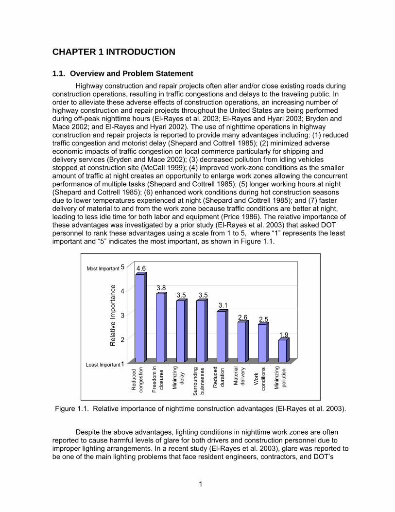
construction operations, resulting in traffic congestions and delays to the traveling public. In order to alleviate these adverse effects of construction operations, an increasing number of highway construction and repair projects throughout the United States are being performed during off-peak nighttime hours (El-Rayes et al. 2003; El-Rayes and Hyari 2003; Bryden and Mace 2002; and El-Rayes and Hyari 2002). The use of nighttime operations in highway construction and repair projects is reported to provide many advantages including: (1) reduced traffic congestion and motorist delay (Shepard and Cottrell 1985); (2) minimized adverse economic impacts of traffic congestion on local commerce particularly for shipping and delivery services (Bryden and Mace 2002); (3) decreased pollution from idling vehicles stopped at construction site (McCall 1999); (4) improved work-zone conditions as the smaller amount of traffic at night creates an opportunity to enlarge work zones allowing the concurrent performance of multiple tasks (Shepard and Cottrell 1985); (5) longer working hours at night (Shepard and Cottrell 1985); (6) enhanced work conditions during hot construction seasons due to lower temperatures experienced at night (Shepard and Cottrell 1985); and (7) faster delivery of material to and from the work zone because traffic conditions are better at night, leading to less idle time for both labor and equipment (Price 1986). The relative importance of these advantages was investigated by a prior study (El-Rayes et al. 2003) that asked DOT personnel to rank these advantages using a scale from 1 to 5, where “1” represents the least important and “5” indicates the most important, as shown in Figure 1.1.
4.6
3.83.5 3.5
3.1
2.6 2.5
1.9
1
2
3
4
5
Rel
ativ
e Im
porta
nce
Red
uced
cong
estio
n
Free
dom
incl
osur
es
Min
imzi
ngde
lay
Surr
ound
ing
buis
ness
es
Red
uced
dura
tion
Mat
eria
lde
liver
y
Wor
kco
nditio
ns
Min
imzi
ngpo
llutio
n
Least Important
Most Important
Figure 1.1. Relative importance of nighttime construction advantages (El-Rayes et al. 2003).
Despite the above advantages, lighting conditions in nighttime work zones are often
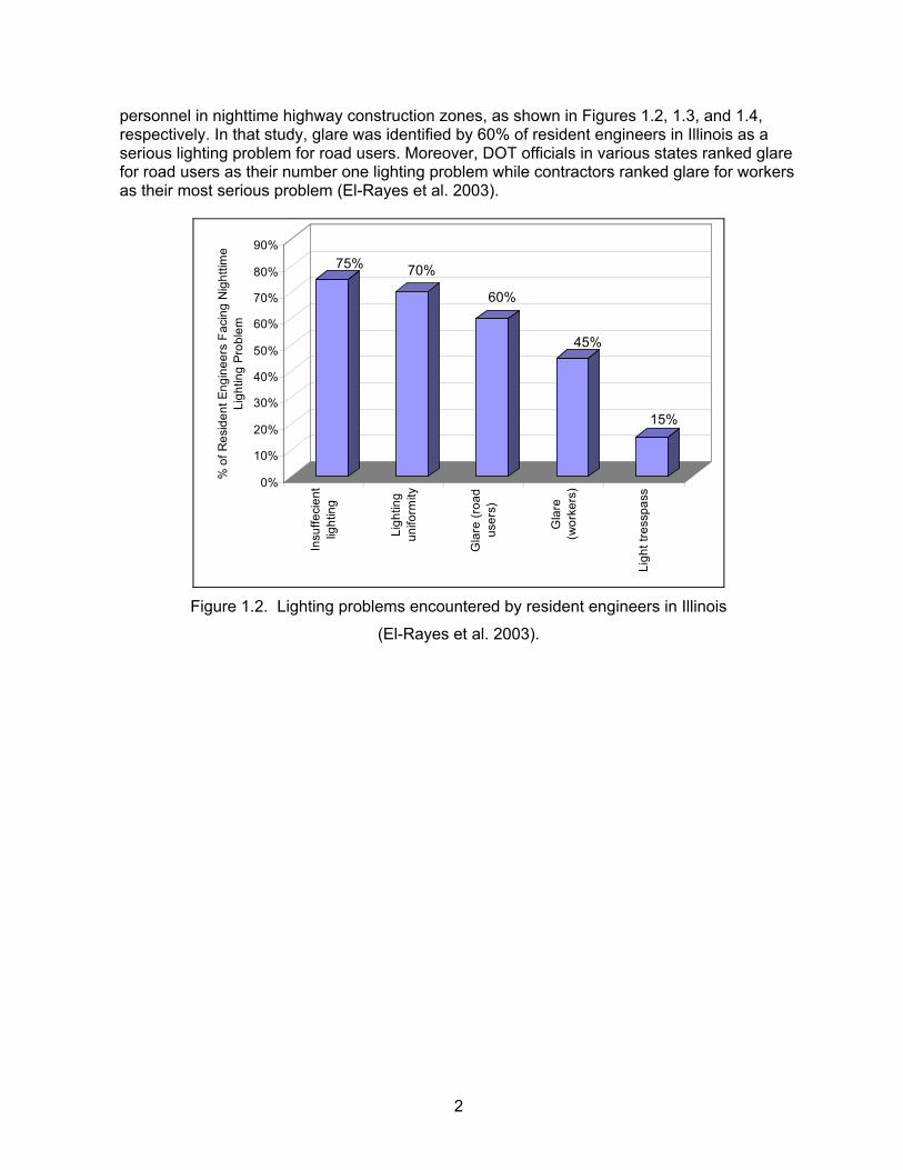
reported to cause harmful levels of glare for both drivers and construction personnel due to improper lighting arrangements. In a recent study (El-Rayes et al. 2003), glare was reported to be one of the main lighting problems that face resident engineers, contractors, and DOT’s
2
personnel in nighttime highway construction zones, as shown in Figures 1.2, 1.3, and 1.4, respectively. In that study, glare was identified by 60% of resident engineers in Illinois as a serious lighting problem for road users. Moreover, DOT officials in various states ranked glare for road users as their number one lighting problem while contractors ranked glare for workers as their most serious problem (El-Rayes et al. 2003).
75% 70%
60%
45%
15%
0%
10%
20%
30%
40%
50%
60%
70%
80%
90%
% o
f Res
iden
t Eng
inee
rs F
acin
g N
ight
time
Ligh
ting
Prob
lem
Insu
ffeci
ent
light
ing
Ligh
ting
unifo
rmity
Gla
re (r
oad
user
s)
Gla
re(w
orke
rs)
Ligh
t tre
sspa
ss
Figure 1.2. Lighting problems encountered by resident engineers in Illinois
(El-Rayes et al. 2003).

3
78% 78%
74%70%
65%
48%
43%
35%30% 30%
22% 22%17%
0%
10%
20%
30%
40%
50%
60%
70%
80%
90%
% o
f Con
tract
ors
Faci
ng N
igtti
me
Ligh
ting
Pro
blem
Gla
re "w
orke
rs"
Uni
form
ity
Gla
re "r
oad
user
s"
Insu
ffici
ent
light
ing
Pla
cem
ent o
feq
uipm
ent
Cos
t of l
ight
ing
Mob
ility
of
equi
pmen
t
Ret
rofit
Con
st.
equi
pmen
t
Avai
labi
lity
ofeq
uipm
ent
Exp
erie
nce
inde
sign
Tres
pass
Ligh
ting
desi
gnto
ol
Equ
ipm
ent
relia
bilit
y
Figure 1.3. Lighting problems encountered by contractors (El-Rayes et al. 2003).
88%
69%
50%
44%
31%
0%
10%
20%
30%
40%
50%
60%
70%
80%
90%
% o
f DO
Ts S
elec
ting
Nig
httim
e Li
ghtti
ng P
robl
em
Glare "roadusers"
Insufficientlighting
Lightinguniformity
Glare"workers"
Light trespass
Figure 1.4. Lighting problems reported by DOTs in nighttime construction
(El-Rayes et al. 2003).

4
Glare is a term used to describe the sensation of annoyance, discomfort, or loss of visual performance and visibility produced by experiencing luminance in the visual field significantly greater than that to which eyes of the observer are adapted (Triaster 1982). Glare from work zone lighting is reported to be one of the most serious challenges confronting nighttime construction operations as it leads to increased levels of hazards and crashes on and around nighttime construction sites (El-Rayes et al. 2003; Hancher and Taylor 2001; Shepard and Cottrell 1985). Nighttime drivers passing near a nighttime construction zone may find difficulty adjusting to the extreme changes in lighting levels when they travel from a relatively dark roadway environment to a bright lighting condition in the work zone. Similarly, the vision of equipment operators in the work zone may be impaired by bright and direct lighting sources. As such, contractors and resident engineers should exert every possible effort to reduce glare during nighttime operations. The major challenge in minimizing glare is caused by the lack of a practical and objective model that can be used to measure and quantify glare on nighttime construction sites. The lack of such a model often leads to disputes among resident engineers and contractors on what constitutes acceptable or objectionable levels of glare and does not enable them to quantify reductions in glare that can be achieved on site.
1.2. Research Objectives The primary goal of this research is to develop a glare measurement model capable of measuring and quantifying lighting glare during nighttime construction work. To achieve this goal, the main research objectives of this study are to:
(1) Conduct an in-depth comprehensive review of the latest literature on the causes of glare and existing practices that can be used to quantify and control glare during nighttime highway construction.
(2) Identify practical factors that affect the measurement of veiling luminance ratio (glare) in and around nighttime work zones.
(3) Analyze and compare the levels of glare and lighting performance generated by typical lighting arrangements in nighttime highway construction.
(4) Evaluate the impact of lighting design parameters on glare and provide practical recommendations for lighting arrangements to reduce and control lighting glare in and around nighttime work zones.
(5) Develop a practical and safe model that can be utilized by contractors and resident engineers to measure and quantify harmful levels of veiling luminance ratio (glare) experienced by drive-by motorists near nighttime highway construction sites.
(6) Investigate and analyze existing recommendations on the maximum allowable levels of veiling luminance ratio (glare) that can be tolerated by nighttime drivers from various lighting sources, including roadway lighting, headlights of opposite traffic vehicles, and lighting equipment in nighttime work zones.
1.3. Research Methodology A research team led by researchers from the University of Illinois at Urbana-
Champaign and Bradley University jointly investigated the effects of veiling luminance ratio (glare) on the traveling public. The team conducted a review of the literature to establish baseline knowledge of existing research in evaluating and calculating the veiling luminance ratio (glare). In addition, the team visited several nighttime construction sites in Illinois. These visits were conducted to identify practical factors that affect the measurement of glare in and around nighttime work zones. The knowledge gathered from the literature and the site visits were used to develop and refine a practical model for quantifying the veiling luminance ratio
5
(glare) that is experienced by drive-by motorists in adjacent lanes to nighttime highway construction zones.
The research team also conducted several field tests to analyze and compare the levels of glare and lighting performance generated by typical lighting arrangements in nighttime highway construction. The test results enabled the research team to provide practical recommendations for lighting arrangements to reduce and control lighting glare in and around nighttime work zones. Furthermore, the team used the field tests in generating regression analysis models that are integrated in the developed model. These regression models were designed to accurately calculate the vertical illuminance values experienced by drivers in adjacent lanes to the work zone based on the measured values at safe locations inside the work zone. The research team also evaluated existing studies and recommendations on the maximum allowable level of veiling luminance ratio that can be tolerated by nighttime motorists.
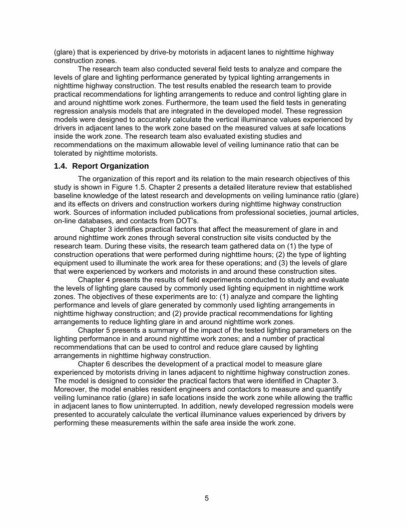
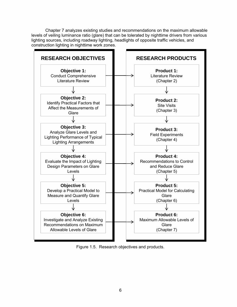
1.4. Report Organization The organization of this report and its relation to the main research objectives of this
study is shown in Figure 1.5. Chapter 2 presents a detailed literature review that established baseline knowledge of the latest research and developments on veiling luminance ratio (glare) and its effects on drivers and construction workers during nighttime highway construction work. Sources of information included publications from professional societies, journal articles, on-line databases, and contacts from DOT’s.
Chapter 3 identifies practical factors that affect the measurement of glare in and around nighttime work zones through several construction site visits conducted by the research team. During these visits, the research team gathered data on (1) the type of construction operations that were performed during nighttime hours; (2) the type of lighting equipment used to illuminate the work area for these operations; and (3) the levels of glare that were experienced by workers and motorists in and around these construction sites.
Chapter 4 presents the results of field experiments conducted to study and evaluate the levels of lighting glare caused by commonly used lighting equipment in nighttime work zones. The objectives of these experiments are to: (1) analyze and compare the lighting performance and levels of glare generated by commonly used lighting arrangements in nighttime highway construction; and (2) provide practical recommendations for lighting arrangements to reduce lighting glare in and around nighttime work zones.
Chapter 5 presents a summary of the impact of the tested lighting parameters on the lighting performance in and around nighttime work zones; and a number of practical recommendations that can be used to control and reduce glare caused by lighting arrangements in nighttime highway construction.
Chapter 6 describes the development of a practical model to measure glare experienced by motorists driving in lanes adjacent to nighttime highway construction zones. The model is designed to consider the practical factors that were identified in Chapter 3. Moreover, the model enables resident engineers and contactors to measure and quantify veiling luminance ratio (glare) in safe locations inside the work zone while allowing the traffic in adjacent lanes to flow uninterrupted. In addition, newly developed regression models were presented to accurately calculate the vertical illuminance values experienced by drivers by performing these measurements within the safe area inside the work zone.
6
Chapter 7 analyzes existing studies and recommendations on the maximum allowable levels of veiling luminance ratio (glare) that can be tolerated by nighttime drivers from various lighting sources, including roadway lighting, headlights of opposite traffic vehicles, and construction lighting in nighttime work zones.
Figure 1.5. Research objectives and products.
Objective 1:Conduct Comprehensive
Literature Review
Objective 2:Identify Practical Factors that Affect the Measurements of
Glare
Objective 3:Analyze Glare Levels and
Lighting Performance of Typical Lighting Arrangements
Objective 4:Evaluate the Impact of Lighting Design Parameters on Glare
Levels
Objective 5:Develop a Practical Model to Measure and Quantify Glare
Levels
Objective 6:Investigate and Analyze Existing Recommendations on Maximum
Allowable Levels of Glare
Product 1:Literature Review
(Chapter 2)
Product 2:Site Visits
(Chapter 3)
Product 3:Field Experiments
(Chapter 4)
Product 4:Recommendations to Control
and Reduce Glare(Chapter 5)
Product 5:Practical Model for Calculating
Glare(Chapter 6)
Product 6:Maximum Allowable Levels of
Glare(Chapter 7)
RESEARCH OBJECTIVES RESEARCH PRODUCTS
7
CHAPTER 2 LITERATURE REVIEW 2. 2
An extensive literature review was conducted to investigate and study existing research on glare in nighttime highway construction. The following sections provide a brief summary of the reviewed literature on (1) lighting requirements for nighttime highway construction; (2) causes of glare in nighttime work zones; (3) types of glare; (4) glare measurements; and (5) available standards and recommendations for glare control.
2.1. Lighting Requirements for Nighttime Highway Construction Lighting conditions in nighttime work zones need to satisfy a number of important
lighting design requirements including: (1) illuminance; (2) light uniformity; (3) glare; (4) light trespass; and (5) visibility. The following sections describe these important lighting requirements.
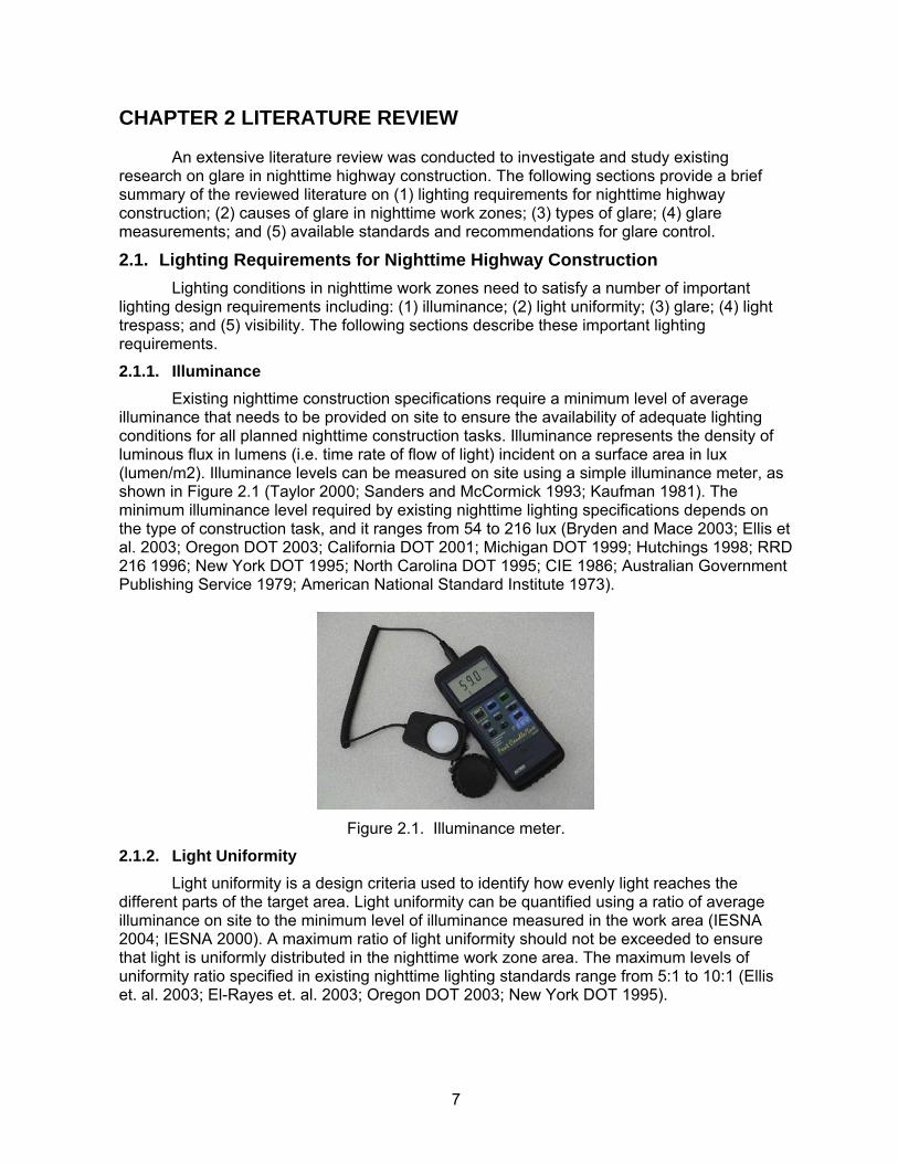
2.1.1. Illuminance Existing nighttime construction specifications require a minimum level of average
illuminance that needs to be provided on site to ensure the availability of adequate lighting conditions for all planned nighttime construction tasks. Illuminance represents the density of luminous flux in lumens (i.e. time rate of flow of light) incident on a surface area in lux (lumen/m2). Illuminance levels can be measured on site using a simple illuminance meter, as shown in Figure 2.1 (Taylor 2000; Sanders and McCormick 1993; Kaufman 1981). The minimum illuminance level required by existing nighttime lighting specifications depends on the type of construction task, and it ranges from 54 to 216 lux (Bryden and Mace 2003; Ellis et al. 2003; Oregon DOT 2003; California DOT 2001; Michigan DOT 1999; Hutchings 1998; RRD 216 1996; New York DOT 1995; North Carolina DOT 1995; CIE 1986; Australian Government Publishing Service 1979; American National Standard Institute 1973).
Figure 2.1. Illuminance meter.
2.1.2. Light Uniformity Light uniformity is a design criteria used to identify how evenly light reaches the
different parts of the target area. Light uniformity can be quantified using a ratio of average illuminance on site to the minimum level of illuminance measured in the work area (IESNA 2004; IESNA 2000). A maximum ratio of light uniformity should not be exceeded to ensure that light is uniformly distributed in the nighttime work zone area. The maximum levels of uniformity ratio specified in existing nighttime lighting standards range from 5:1 to 10:1 (Ellis et. al. 2003; El-Rayes et. al. 2003; Oregon DOT 2003; New York DOT 1995).
8
2.1.3. Glare To minimize its negative impact on road users and construction workers, a maximum
level of glare should not be exceeded in and around the highway construction zone. Glare can be defined as the sensation of annoyance, discomfort or loss of visual performance and visibility due to experiencing luminance in the visual field significantly greater than that to which the eyes of the observer are adapted (Pritchard 1999). Glare can be quantified using the veiling luminance ratio, which is determined by calculating the ratio of the veiling luminance to the average pavement luminance in and around the work zone (IESNA 2004; IESNA 2000). The rationale behind using this ratio rather than the absolute veiling luminance is due to the fact that the sensation of glare is not only dependent on the amount of veiling luminance reaching the driver’s eyes as an absolute value, but also on the lighting level at which the driver’s eyes are adapted to before being exposed to that amount of glare. It should be noted that available lighting standards do not specify a maximum veiling luminance ratio for nighttime construction; however, IESNA recommends a maximum ratio of 0.4 to control glare caused by permanent roadway lighting (IESNA 2004; IESNA 2000).
As previously mentioned, glare can be quantified as a ratio of veiling luminance to the average pavement luminance. Veiling luminance depends on the levels of vertical illuminance that reach the driver’s eyes and it can be measured on site using an illuminance meter (see Figure 2.1) while the pavement luminance can be measured using a luminance meter as shown in Figure 2.2 (Triaster 1982). Pavement luminance can be defined as a quantitative measure of the surface brightness measured in candelas per square meter or foot lamberts (Triaster 1982). Pavement luminance controls the magnitude of the sensation of an object which the brain receives. It depends on several factors including (1) the amount of light incident on the pavement; (2) the reflection characteristics of the pavement surface; (3) relative angle from which the light strikes the surface; and (4) location of the observer.
Figure 2.2. Luminance meter.
Pavement surfaces reflect light towards the drivers using two mechanisms; specularity
and diffusion characteristics (see Figure 2.3). An ideal specular surface would reflect the entire incident light at a point at an angle of reflection exactly equal to the angle of incidence. Examples of ideally specular surfaces include mirrors, highly-polished metal surfaces, and the surface of liquids. In total opposite to an ideally specular surface, a perfectly diffuse surface reflects light as a cosine function of the incident angle. A perfectly diffuse surface would appear equally bright to an observer from any viewing angle. Examples of ideally diffuse

9
surfaces include walls finished with flat white paint at incident angles close to zero degrees (King 1976).
Although one of these two mechanisms is primarily controlling light reflection for a given surface, no pavement surface will act as an ideal diffuser or specular but rather as a combination of these two forms. Portland cement concrete surfaces essentially utilize a diffuse reflection mode while asphalt concrete surfaces mainly act as a specular one. Pavement reflectance properties depend, among other factors, on the surface characteristics, the color, and the roughness of the surface. Because of their light-colored aggregates, concrete surfaces have initial higher reflectance values than asphalt surfaces.
Figure 2.3. Comparison between specular and diffuse reflections.
To explain the mixed influences of the specular and diffusion properties of a surface,
consider a single luminaire on the side of a roadway, which would produce a single luminous patch on the pavement surface. To the driver, this luminous will produce a patch with the form of a “T” with the tail extending toward the observer (see Figure 2.4). The size, shape, and luminance properties of the “T” depend mainly on the reflectance properties of the surface. For a diffusive-dominant surface, the head of the “T” predominates and only a short tail would appear. For a specular-dominant surface, the head of the “T” will be small and the tail very long. For a wet surface, the head may not be visible and the tail may become elongated.
Ideal Specular Reflection Perfectly Diffuse Reflection
θ1 θ2
θ1=θ2
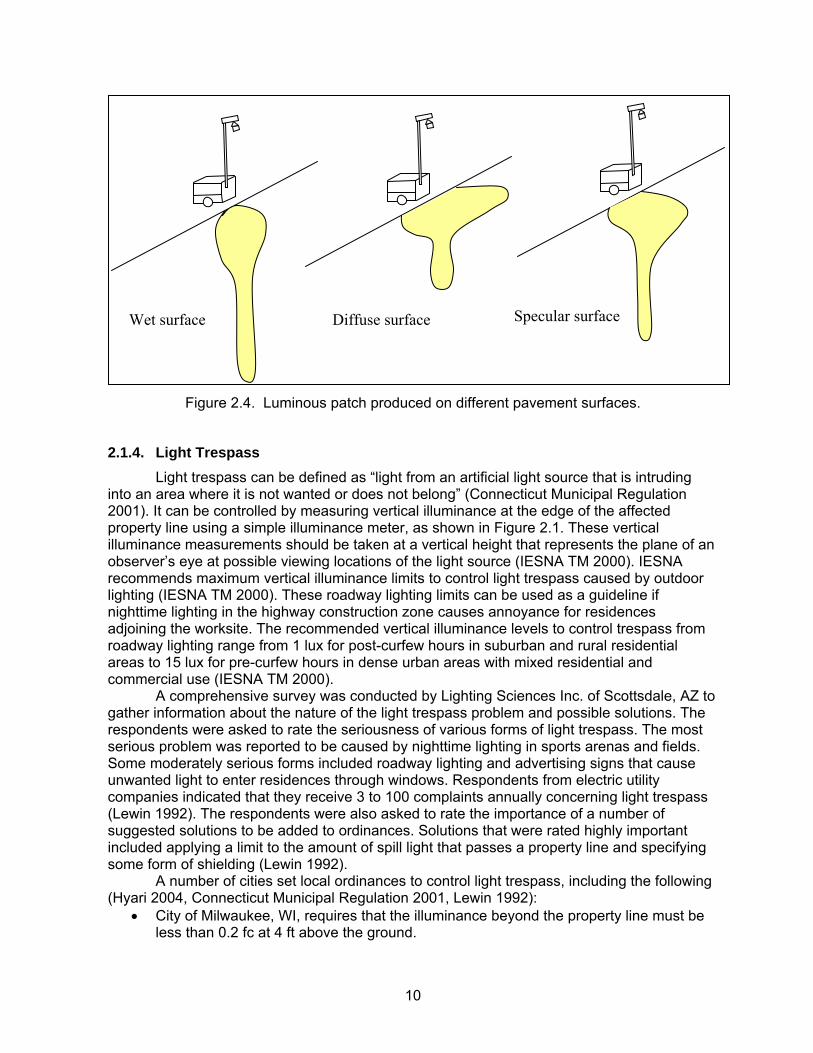
10
Figure 2.4. Luminous patch produced on different pavement surfaces.
2.1.4. Light Trespass Light trespass can be defined as “light from an artificial light source that is intruding into an area where it is not wanted or does not belong” (Connecticut Municipal Regulation 2001). It can be controlled by measuring vertical illuminance at the edge of the affected property line using a simple illuminance meter, as shown in Figure 2.1. These vertical illuminance measurements should be taken at a vertical height that represents the plane of an observer’s eye at possible viewing locations of the light source (IESNA TM 2000). IESNA recommends maximum vertical illuminance limits to control light trespass caused by outdoor lighting (IESNA TM 2000). These roadway lighting limits can be used as a guideline if nighttime lighting in the highway construction zone causes annoyance for residences adjoining the worksite. The recommended vertical illuminance levels to control trespass from roadway lighting range from 1 lux for post-curfew hours in suburban and rural residential areas to 15 lux for pre-curfew hours in dense urban areas with mixed residential and commercial use (IESNA TM 2000). A comprehensive survey was conducted by Lighting Sciences Inc. of Scottsdale, AZ to gather information about the nature of the light trespass problem and possible solutions. The respondents were asked to rate the seriousness of various forms of light trespass. The most serious problem was reported to be caused by nighttime lighting in sports arenas and fields. Some moderately serious forms included roadway lighting and advertising signs that cause unwanted light to enter residences through windows. Respondents from electric utility companies indicated that they receive 3 to 100 complaints annually concerning light trespass (Lewin 1992). The respondents were also asked to rate the importance of a number of suggested solutions to be added to ordinances. Solutions that were rated highly important included applying a limit to the amount of spill light that passes a property line and specifying some form of shielding (Lewin 1992). A number of cities set local ordinances to control light trespass, including the following (Hyari 2004, Connecticut Municipal Regulation 2001, Lewin 1992):
• City of Milwaukee, WI, requires that the illuminance beyond the property line must be less than 0.2 fc at 4 ft above the ground.
Wet surface Diffuse surface Specular surface

11
• City of Greenwich, CT, requires that (1) all exterior lights be shielded; (2) lights adjacent to businesses must not be visible from a height of greater than 5 ft while those adjacent to residential areas must not be visible at any height; and (3) intensity of lighting at property line must not exceed 0.5 fc for businesses or 0.1 fc for residences.
• County of San Diego, CA, requires that illuminance levels caused by spill light shall not exceed 0.2 fc; which is equivalent to the amount of illuminance from moonlight, in both the horizontal and vertical planes at a point 1.5 m (5 ft) inside the owner’s property line.
• Village of Skokie, IL, defines light trespass to be light from a roadway lighting system falling on adjacent properties with an intensity of more than 0.3 fc.
• County of Milford, CT, limits the maximum allowable illuminance on the edge of a property line to 0.1 fc and 0.5 fc for residentially and commercially zoned properties, respectively.
• County of Watertown, CT, prevents the location of any lighting within 5 ft of any property lines.
The Illuminating Engineering Society of North America (IESNA) recommends limits for vertical illumination that reaches a property. Table 2.1 shows this society’s limits for light trespass which represent the maximum allowed vertical illuminance in the plane of an observer’s eye at possible viewing locations of the light source, which are recommended to be measured at the edge of the property line (Hyari 2004, IESNA TM-2000).
Table 2.1. Recommended Light Trespass Limitations (IESNA TM-2000)
Environmental Zone Pre-Curfew Limitations*
Post-Curfew Limitations*
Areas of low ambient brightness (suburban and rural residential areas where roadway lighting may be lighted to typical residential standards)
3.0 (0.3) 1.0 (0.1)
Areas of medium ambient brightness (e.g. urban residential areas where roadway lighting will normally be traffic route standards)
8.0 (0.8) 3.0 (0.3)
Areas of high ambient brightness (e.g. dense urban areas with mixed residential and commercial use with a high level of nighttime activity)
15.0 (1.5) 6.0 (0.6)
*Lux (footcandles) values on a plane perpendicular to the line of sight to the luminaire (s).
2.1.5. Visibility Visibility is often considered to be a more valid criterion for roadway lighting design than luminance and illuminance (Janoff et al. 1989). This is mainly due to the findings of research studies that indicated the existence of a correlation between visibility and both
12
nighttime safety and human visual performance, and the inability to establish such a correlation between luminance or illuminance and these factors (Janoff et al. 1989). Despite its significance, no research has been directed towards overcoming the difficulty of measuring visibility (Ellis et al. 1995). Currently there are a limited number of devices to measure visibility in controlled environments such as laboratories, all of which are based on reducing the illuminance of the scene until a predetermined object called the critical detail, can barely be seen (Kaufman and Christensen 1987). A quantitative measure of Visibility is the Visibility Index, which can be calculated using Equation 2.1 (Janoff et al. 1989). VI= C X RCS X DGF (2.1) Where, C = physical contrast; RCS = relative contrast sensitivity; and DGF = disability glare factor. Visibility is also an important criterion in roadway lighting design because humans use luminance contrast to distinguish between the target object and the background. As such, visibility is affected by both glare and contrast sensitivity (Janoff et al. 1989). Contrast sensitivity is “the ability to detect luminance difference,” while contrast can be defined as “the relationship between luminance of an object and its immediate background” and it is given by the following equation (Kaufman 1981). Contrast = (Lo-Li)/Li (2.2) Where, Lo = luminance of the object; and Li = luminance of the background.
2.2. Causes of Glare in Nighttime Work Zone Glare from work zone lighting is reported to be one of the most serious challenges confronting nighttime construction operations as it leads to increased levels of hazards and crashes on and around nighttime construction sites (El-Rayes et al. 2003; Hancher and Taylor 2001; Cottrell 1999; Shepard and Cottrell 1985). The main causes of glare in nighttime work zones that were reported in the literature review include: glare from fixed road lighting, glare from vehicles’ headlamps, and glare from construction and lighting equipments (Porter et al. 2005; IESNA 2004; Ellis et al. 2003; Bullough et al. 2002; IESNA 2000; Cottrell 1999; Mace et al. 2001; Schieber 1998; Ellis and Amos 1996). Several research studies have reported that roadway lighting can cause glare for drivers and pedestrians. The effect of glare from roadway lighting increases with: (1) the increase of the glare source's luminance; (2) the decrease of the pavement luminance; and (3) the decrease of the glare angle between the light source and the line of sight of the observer (IESNA 2004; Bullough et al. 2002; Mace et al. 2001; IESNA 2000). The glare angle and its impact on the overall levels of glare experienced by drivers are affected by three factors: (1) the distance between the driver and the light source; (2) the height of the light source relative to the height of the observer; and (3) the direction in which the light is aimed (Bryden and Mace 2002; Ellis and Amos 1996). In urban and semi-urban environments where roadway lights are available, there are fewer glare problems because of the availability of the road lights that increase the pavement luminance (Ellis et al. 2003). As for rural areas, glare is a serious problem because of the sudden shift from a dark environment to a well lit one and then back to dark again when passing through a construction zone. The IESNA (IESNA 2004; IESNA 2000) recommends the use of a veiling luminance ratio as a method to measure and
13
control glare in roadway lighting design. A maximum veiling luminance ratio of 0.4 is recommended as a threshold to control glare at nighttime driving by the IESNA (2004). Vehicle headlights are also a major cause of glare in nighttime driving (Mace et al. 2001). Several factors affect the levels of glare caused by vehicles headlights including: (1) intensity of light produced by the headlights; (2) illuminance levels that reach the drivers eyes from the headlights of vehicles on the opposite direction; (3) angle between the headlights and the line of sight of the driver traveling on the opposite direction which depends on the geometry of the road (i.e., median and lane width); (4) photometric distribution of the headlights’ high and low beam; (5) aiming standards of the headlights; and (6) headlights height (Mace et al. 2001). Glare is also caused by lighting in nighttime construction zones (El-Rayes and Hyari 2005; Hyari 2004; Ellis et al. 2003; El-Rayes et al. 2003; Bryden and Mace 2002; Ellis and Amos 1996; Amos 1994). Several factors affect glare levels in and around nighttime construction zones including: (1) type and intensity of the utilized lighting equipment; (2) location of the nighttime lights in the nighttime work zone and their proximity to drivers and construction personnel; (3) aiming angle of the luminaries; and (4) height of the light sources on site (El-Rayes and Hyari 2005; El-Rayes et al. 2003). Moreover, the problem of glare to motorists from highway construction was found to be acute when adjacent lanes for the construction area were opened to traffic (Ellis et al. 2003).
2.3. Types of Glare Glare is a term used to describe the sensation of annoyance, discomfort or loss of visual performance and visibility produced by experiencing luminance in the visual field significantly greater than that to which eyes of the observer are adapted (Triaster 1982). Glare can also be described as the excessive contrast between bright and dark areas in the visual field. The bright object by itself may not cause glare; however, glare will be experienced if a dark background exists with the bright object. Glare can be classified based on its source as either direct or reflected (Sanders and McCormick 1993) and based on its impact as discomfort, disabling or blinding glare (Porter et al. 2005; Bullough et al. 2002; Mace et al. 2001; Schieber 1998; Sanders and McCormick 1993).
2.3.1. Direct and Reflected Glare Direct glare is mainly caused by direct observation of high luminances in the visual environment of the observer. Examples of direct glare include an insufficiently shielded luminaire, headlights, and taillights (Porter et al. 2005; Mace et al. 2001; Schieber 1998; Sanders and McCormick 1993). Reflected glare is caused by the reflection of light from a surface (Sanders and McCormick 1993). Examples of reflected glare include reflected light from polished surfaces such as the steel or aluminum doors on tractor trailers or a rear-view mirror at night that reflect light toward the driver’s eye. Reflected glare can be further classified into four main types: (1) specular, which is caused by reflected light from smooth or polished surface; (2) spread, which is caused when the reflecting surface is brushed or etched; (3) diffuse; when the light is reflected from flat-painted or matte surface; and (4) compound, when there is combination of the first three types (Sanders and McCormick 1993).
2.3.2. Discomfort, Disabling and Blinding Glare Glare can also be classified based on its impact on the observers into three types: discomfort, disabling and blinding (Porter et al. 2005; Bullough et al. 2002; Mace et al. 2001; Schieber 1998; Sanders and McCormick 1993). Discomfort glare may result in discomfort, annoyance, pain, and fatigue that may have a deleterious effect on vision (Porter et al. 2005; Bryden and Mace 2002, Mace et al. 2001). Discomfort glare depends on three main factors (1) size, luminance, and number of glare sources; (2) the background luminance; and (3) the
14
angle between the observer’s line of site and the source of glare (Mace et al. 2001; Schieber 1998; Amos 1994). Disabling glare on the other hand is often reported at levels of illumination well above those of discomfort glare (Schieber 1998). Disabling glare results from light scatter within the eye that effectively reduces the visibility of objects (Porter et al. 2005; Bryden and Mace 2002; Mace et al. 2001; Schieber 1998; Sanders and McCormick 1993). Disabling glare, also known as veiling luminance, has strong effect on visibility as it produces a reduction in the visibility distance of low contrast objects (Mace et al. 2001). When an intense light is presented near the line of sight of the observer, the light will scatter in the eye, which overlays the retinal image of an object and reduces the contrast of the retinal image. This scattered light is described as the veiling luminance. Also, the reduction of the object’s contrast can reach a threshold where the object is hardly visible. This effect is very important at nighttime when contrast sensitivity is low and one or more bright lights are near the line of sight such as vehicles headlights, streetlights, or construction equipment lights (CIE 2002). There are three factors that affect disabling glare: (1) illuminance incident on the observer eye from the glare source; (2) age of the observer; and (3) the angle between the observer’s line of site and the center of the glare source. Disabling glare is evaluated by comparing it to the adaptation luminance of the motorists which is considered by IESNA to be the pavement luminance levels (Mace et al. 2001; IESNA 2004; IESNA 2000). The age of the observer is a main factor that affects the measurement of disabling glare. Typically, people's visual faculties decline with age and tend to be more farsighted. The cellular lens of the eyes continues to grow over time, especially the outer layer of the lens. The growth of the cells will increase the thickness of the lens which is the major cause for farsightedness in the elderly, and the thickness will increase the scattering of light passing through the lens. The scattering of the light will cause a veiling luminance over the retinal image and blurs the image on the retina. Also the muscles of the pupil begin to atrophy with age, which will decrease the range and speed of the pupil adjustment over different illumination levels. All these factors will reduce the amount of illumination that reaches the retina and reduce visual acuity (Sanders and McCormick 1993). Weale (1961) demonstrated a 50% reduction of retinal illumination for 50-year old individuals compared to 20-year olds. This further increases to 66% reduction at age 60. Moreover, the National Center for Health Statistics (1977) shows an increase in the percentage of people with defective visual acuity from 0.7% between age 35 to 44 up to 14% between age 65 to 74 (Sanders and McCormick 1993). The decrease of the speed of the pupil adjustment over different illumination levels and the increase of the light scattering through the eye will increase the sensitivity to disabling glare over time (Sanders and McCormick 1993). Blinding glare is also called dazzling glare. It causes temporary vision deficiencies such as the effect experienced when staring into the sun. Blinding glare has a long term-effect even after the light source is removed (Sanders and McCormick 1993). It causes the interruption of vision due to very bright visual scenes, such as a sunny beach, presumably due to pupillary spasm by over contraction (Vos 2003). Blinding glare is reported by Vos (2003) to be functional protection against retinal over-exposure which might lead to temporary or even permanent blindness due to photochemical light damage or to retinal burn.
2.4. Glare Measurements Several studies in the literature have reported various methods to measure and quantify discomfort and disabling glare. The following three sections highlight existing methods to measure these two types of glare as well as available methods to quantify pavement/adaptation luminance which is essential in measuring both types of glare.
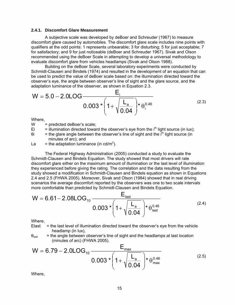
15
2.4.1. Discomfort Glare Measurement A subjective scale was developed by deBoer and Schreuder (1967) to measure discomfort glare caused by automobiles. The discomfort glare scale includes nine points with qualifiers at the odd points: 1 represents unbearable; 3 for disturbing; 5 for just acceptable; 7 for satisfactory; and 9 for just noticeable (deBoer and Schreuder 1967). Sivak and Olson recommended using the deBoer Scale in attempting to develop a universal methodology to evaluate discomfort glare from vehicles headlamps (Sivak and Olson 1988). Building on the deBoer Scale, several laboratory experiments were conducted by Schmidt-Clausen and Bindels (1974) and resulted in the development of an equation that can be used to predict the value of deBoer scale based on: the illumination directed toward the observer’s eye, the angle between observer’s line of sight and the glare source, and the adaptation luminance of the observer, as shown in Equation 2.3.
46.0i
a
i
*04.0
L1*003.0
ELOG0.20.5Wθ⎟
⎟⎠
⎞⎜⎜⎝
⎛+
−= (2.3)
Where, W = predicted deBoer’s scale; Ei = illumination directed toward the observer’s eye from the ith light source (in lux); θi = the glare angle between the observer’s line of sight and the ith light source (in
minutes of arc); and La = the adaptation luminance (in cd/m2). The Federal Highway Administration (2005) conducted a study to evaluate the Schmidt-Clausen and Bindels Equation. The study showed that most drivers will rate discomfort glare either on the maximum amount of illumination or the last level of illumination they experienced before giving the rating. The correlation and the data resulting from the study showed a modification in Schmidt-Clausen and Bindels equation as shown in Equations 2.4 and 2.5 (FHWA 2005). Moreover, Sivak and Olson (1984) showed that in real driving scenarios the average discomfort reported by the observers was one to two scale intervals more comfortable than predicted by Schmidt-Clausen and Bindels Equation.
46.0last
a
last10
*04.0
L1*003.0
ELOG08.261.6Wθ⎟
⎟⎠
⎞⎜⎜⎝
⎛+
−= (2.4)
Where, Elast = the last level of illumination directed toward the observer’s eye from the vehicle
headlamp (in lux), θlast = the angle between observer’s line of sight and the headlamps at last location
(minutes of arc) (FHWA 2005).
46.0max
a
max10
*04.0
L1*003.0
ELOG0.279.6Wθ⎟
⎟⎠
⎞⎜⎜⎝
⎛+
−= (2.5)
Where,
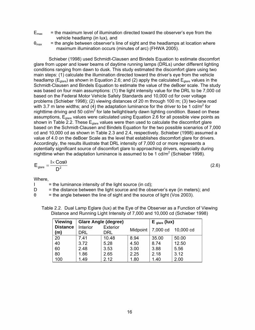
16
Emax = the maximum level of illumination directed toward the observer’s eye from the vehicle headlamp (in lux), and
θmax = the angle between observer’s line of sight and the headlamps at location where maximum illumination occurs (minutes of arc) (FHWA 2005).
Schieber (1998) used Schmidt-Clausen and Bindels Equation to estimate discomfort glare from upper and lower beams of daytime running lamps (DRLs) under different lighting conditions ranging from dawn to dusk. This study estimated the discomfort glare using two main steps: (1) calculate the illumination directed toward the driver’s eye from the vehicle headlamp (Eglare) as shown in Equation 2.6; and (2) apply the calculated Eglare values in the Schmidt-Clausen and Bindels Equation to estimate the value of the deBoer scale. The study was based on four main assumptions: (1) the light intensity value for the DRL to be 7,000 cd based on the Federal Motor Vehicle Safety Standards and 10,000 cd for over voltage problems (Schieber 1998); (2) viewing distances of 20 m through 100 m; (3) two-lane road with 3.7 m lane widths; and (4) the adaptation luminance for the driver to be 1 cd/m2 for nighttime driving and 50 cd/m2 for late twilight/early dawn lighting condition. Based on these assumptions, Eglare values were calculated using Equation 2.6 for all possible view points as shown in Table 2.2. These Eglare values were then used to calculate the discomfort glare based on the Schmidt-Clausen and Bindels Equation for the two possible scenarios of 7,000 cd and 10,000 cd as shown in Table 2.3 and 2.4, respectively. Schieber (1998) assumed a value of 4.0 on the deBoer Scale as the level that establishes discomfort glare for drivers. Accordingly, the results illustrate that DRL intensity of 7,000 cd or more represents a potentially significant source of discomfort glare to approaching drivers, especially during nighttime when the adaptation luminance is assumed to be 1 cd/m2 (Schieber 1998).
2glare DCosIE θ×
= (2.6)
Where, I = the luminance intensity of the light source (in cd); D = the distance between the light source and the observer’s eye (in meters); and θ = the angle between the line of sight and the source of light (Vos 2003).
Table 2.2. Dual Lamp Eglare (lux) at the Eye of the Observer as a Function of Viewing Distance and Running Light Intensity of 7,000 and 10,000 cd (Schieber 1998)
Glare Angle (degree) E glare (lux) Viewing Distance (m)
Interior DRL
Exterior DRL Midpoint 7,000 cd 10,000 cd
20 7.41 10.48 8.94 35.00 50.00 40 3.72 5.28 4.50 8.74 12.50 60 2.48 3.53 3.00 3.88 5.56 80 1.86 2.65 2.25 2.18 3.12 100 1.49 2.12 1.80 1.40 2.00

17
Table 2.3. Estimated deBoer Discomfort Glare Rating as a Function of Viewing Distance and Background Luminance for 7000 cd Daytime Running Lights (Schieber 1998)
deBoer Scale Adaptation Luminance (cd/m2)
Viewing Distance (m)
Glare Angle (minarc)
E glare (lux)
1 50 20 536 35.00 0.93 2.49 40 270 8.74 1.86 3.43 60 189 3.88 2.41 3.97 80 135 2.18 2.79 4.36 100 108 1.40 3.09 4.65
Table 2.4. Estimated deBoer Discomfort Glare Rating as a Function of Viewing Distance and
Background Luminance for 10000 cd Daytime Running Lights (Schieber 1998).
deBore Scale Adaptation Luminance (cd/m2)
Viewing Distance (m)
Glare Angle (minarc)
E glare (lux)
1 50 20 536 50.00 0.62 2.19 40 270 12.50 1.55 3.12 60 189 5.56 2.09 3.66 80 135 3.12 2.48 4.05 100 108 2.00 2.78 4.34
Vos (2003) proposed a method to measure discomfort glare due to roadway lighting using a similar approach to that of the deBoer Scale. This approach used a Glare Control Mark (GM) that can be calculated using Equation 2.7. The GM depends on the number, height, color, directional radiation pattern of the light sources, the projected area of the luminaires, the light intensity in the direction of an approaching car driver, and the average road luminance. Vos (2003) suggested the use of a scale to relate GM values to discomfort levels, where GM = 1 represents bad, GI = 3 is inadequate, GI = 5 is fair, GI = 7 is good, and GI = 9 is excellent.
GM = F + 1.29 log A14 – 3.31 log I10 + 0.97 log Lrd (2.7)
Where, F = a value which is determined by the installation characteristics (number of light points
per km, suspension height, color and directional radiation pattern); A14 = the projected area of the luminaires (in m2) visible at 14° below the horizontal; I10 = the intensity (cd) in the direction of an approaching car driver at 10° below the
horizontal line of view; and Lrd = the average road luminance (cd/m2) (Vos 2003). Moreover, Vos (2003) also proposed a method to measure discomfort glare in interior spaces (see Equation 2.8) using a glare index (GI) that depends on: the luminance and solid angle of the light sources, the luminance of the direct field of view, and the position angle between the light source and the line of sight. Vos (2003) suggested the use of a scale to
18
relate GI values to discomfort levels, where GI = 600 represents intolerable, GI = 150 is uncomfortable, GI = 35 is acceptable and GI = 8 is perceptible.
)(f)L()()L(GI
sc
f
bs
as
seriorint θ×Ω×
= ∑ (2.8)
Where, Ls = the luminance of the light source s; Ωs = the solid angle of the light source s; Lf = the luminance of the direct field of view f; fs (θ) = an empirical weighting function of the position angle θ between light source and line
of sight; and a, b, and c = empirical best fitting values (Vos 2003).
2.4.2. Disabling Glare Measurement The most common formula for quantifying disabling glare was a result of many studies done by Holladay, Stiles and later Stiles and Crawford. It is known as the Stiles-Holladay disabling glare formula for a point glare source as shown in Equation 2.9 (Vos 2003; CIE 2002; Mace et al. 2001).
2glare
eq
E10L
θ
×= (2.9)
Where, Leq = veiling luminance or equivalent veiling background in cd/m2; Eglare = illuminance at the observer’s eye in lux which is caused by the glare source and it
can be calculated using the inverse square law (Equation 2.6); and θ = the angle between the line of sight and the glare source in degrees. The Stiles-Holladay disabling glare formula did not consider the age of the driver and was also limited to angular range of one-degree up to 30-degree (Vos 2003). The International Commission on Illumination - abbreviated as CIE from its French title Commission Internationale de l'Eclairage – set a committee to update Stiles-Holladay equation. The results were three disabling glare equations that are an extension of the classic Stiles-Holladay equation that take into consideration the effect of age and the effect of ocular pigmentation (CIE 2002). The first developed equation is the CIE Age-adjusted Stiles-Holladay Disabling Glare equation, which is the simplest one but has a restricted validity domain of 1° < θ < 30°, as shown in Equation 2.10.
2
4
glare
veil 1*70
Age110HolladayStilesadjustedageEL
θ⎥⎥⎦
⎤
⎢⎢⎣
⎡⎟⎠⎞
⎜⎝⎛+=−−
⎥⎥⎦
⎤
⎢⎢⎣
⎡ (2.10)
Where, Lveil = the veiling luminance (in cd/m2); Eglare = illuminance at the observer’s eye (in lux); Age = the age of the observer (in years); and θ = the angle between the line of sight and the glare source in degrees. The second formula is the CIE Small Angle Disabling Glare equation which extends in the lower angular region to the domain of 0.1° < θ < 30°, as shown in Equation 2.11.
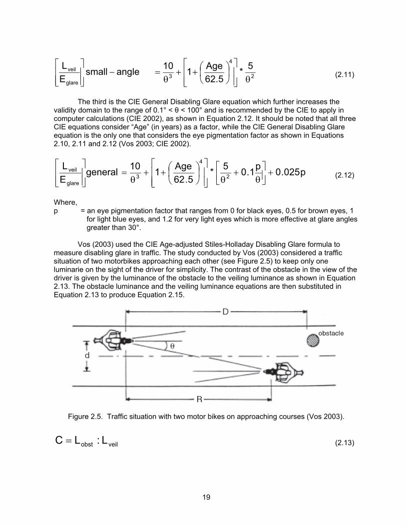
19
2
4
3glare
veil 5*5.62
Age110anglesmallEL
θ⎥⎥⎦
⎤
⎢⎢⎣
⎡⎟⎠⎞
⎜⎝⎛++
θ=−
⎥⎥⎦
⎤
⎢⎢⎣
⎡ (2.11)
The third is the CIE General Disabling Glare equation which further increases the validity domain to the range of 0.1° < θ < 100° and is recommended by the CIE to apply in computer calculations (CIE 2002), as shown in Equation 2.12. It should be noted that all three CIE equations consider “Age” (in years) as a factor, while the CIE General Disabling Glare equation is the only one that considers the eye pigmentation factor as shown in Equations 2.10, 2.11 and 2.12 (Vos 2003; CIE 2002).
p025.0p1.05*5.62
Age110generalEL
2
4
3glare
veil +⎥⎦⎤
⎢⎣⎡
θ+
θ⎥⎥⎦
⎤
⎢⎢⎣
⎡⎟⎠⎞
⎜⎝⎛++
θ=
⎥⎥⎦
⎤
⎢⎢⎣
⎡ (2.12)
Where, p = an eye pigmentation factor that ranges from 0 for black eyes, 0.5 for brown eyes, 1
for light blue eyes, and 1.2 for very light eyes which is more effective at glare angles greater than 30°.
Vos (2003) used the CIE Age-adjusted Stiles-Holladay Disabling Glare formula to measure disabling glare in traffic. The study conducted by Vos (2003) considered a traffic situation of two motorbikes approaching each other (see Figure 2.5) to keep only one luminarie on the sight of the driver for simplicity. The contrast of the obstacle in the view of the driver is given by the luminance of the obstacle to the veiling luminance as shown in Equation 2.13. The obstacle luminance and the veiling luminance equations are then substituted in Equation 2.13 to produce Equation 2.15.
Figure 2.5. Traffic situation with two motor bikes on approaching courses (Vos 2003).
veilobst L:LC = (2.13)
20
⎟⎟
⎠
⎞
⎜⎜
⎝
⎛θ
⎥⎥⎦
⎤
⎢⎢⎣
⎡
⎭⎬⎫
⎩⎨⎧+ρ= 2
reesdeg
4
22 /70
Age1.RI10:
DIC (2.14)
])70/Age(1[10)D/d]/180.([C 4
2
+πρ
= (2.15)
Where, ρ = the reflection factor of the obstacle; I = the headlight intensity; D = the distance from the driver to the obstacle; d = the lateral distance between the two motorbikes. R = the mutual distance between the two motorbikes; Age = the age of the driver; and θ = the glare angle which can also be calculated using Equation 2.16 as follows:
θdegrees = (180/π) d/R (2.16)
A detection distance “D” for the obstacle can be developed from Equation 2.15 as shown in Equation 2.18. Vos (2003) used this equation to illustrate how age influences the distance for detecting an obstacle on the road with the presence of disabling glare. A 25% reflection factor for the obstacle (ρ = 0.25) with a minimum contrast of 25% (C = 0.25) and a 5 meters lateral lane distance (d = 5) was assumed. Based on these assumptions, the detection distance “D” can then be calculated using Equation 2.18.
)]70/Age[1(C10.d)/180(D 4ectiondet +
ρπ= (2.17)
)]70/Age[1(90D
4ectiondet+
= (2.18)
Equation 2.18 shows that the detection distance will be equal to 90 meters for young observers (i.e. 25-year-old), while older observers of 70 and 83 years-old need shorter detection distances of 64 and 52 meters, respectively. Furthermore, Vos (2003) adjusted Equation 2.18 to consider the presence of some extraocular light scatter sources such as a dirty or scratched windshield by doubling the coefficient 10 in the original Stiles-Holladay, as shown in Equation 2.19. This produced shorter detection distances and breaking times as shown in Table 2.5.
)]70/Age[2(90D
4ectiondet+
= (2.19)

21
Table 2.5. Nominal Detection Distance and Braking Time for a Crossing Pedestrian, while Blinded by an Undipped Approaching Motorbike (Vos 2003)
Nominal detection distance (m)
Nominal breaking time (sec)
Young adults 64 2.3 70 years old 52 1.9 83 years old 45 1.6
Another study by Schieber (1998) was conducted to quantify disabling glare from upper and lower beams of daytime running lamps (DRLs) under different lighting conditions ranging from dawn to dusk. This study measured disabling glare using two main steps: (1) calculate the “equivalent veiling luminance” (Lequivalent) based on the illumination that reaches the observer’s eye from the light source (Eglare), the angle between the line of sight and the glare source (θ), and the age of the observer using Equation 2.20; and (2) calculate a threshold for disabling glare that was named (Thresholdelevation) based on the equivalent veiling luminance (Lequivalent) calculated in the first step and the pavement/background luminance (Lbackground) experienced by the driver, as shown in Equation 2.22. Schieber (1998) reported that significant disabling glare can be experienced by drivers when the threshold value exceeds 2 (i.e., Thresholdelevation > 2).
2glare
equivalent
E*kL
θ= (2.20)
Where, θ = the angle between the glare source and the observer’s line of sight (degrees); Eglare = the illumination caused by the glare source at the eye of the observer (lux) calculated
by (Equation 2.6); and k = a variable dependent on the age of the observer and can be calculated using
equation 2.19 (Mace et al. 2001; Schieber 1998).
( )⎟⎟⎠
⎞⎜⎜⎝
⎛⎟⎠⎞
⎜⎝⎛ −−
+=4
4.66inyearsobserverofAge105.9k
(2.21)
( ) equivalentbackgroundbackgroundelevation LLL01.0
01.0Threshold+
= (2.22)
Where, Lbackground = adaptation or pavement luminance; and Lequivalent = equivalent veiling luminance calculated using Equation 2.20. The Schieber study (1998) was based on four main assumptions: (1) the light intensity value for the DRL to be 7,000 cd according to the Federal Motor Vehicle Safety Standards and 10,000 cd in case of over voltage problems; (2) viewing distances of 20 m through 100 m; (3) a two-lane road with 3.7 m lane widths; and (4) the adaptation luminance for the driver to be 1 cd/m2 for nighttime driving and 50 cd/m2 for late twilight/early dawn lighting condition. Based on these assumptions, Eglare values were calculated using Equation 2.6 for all possible
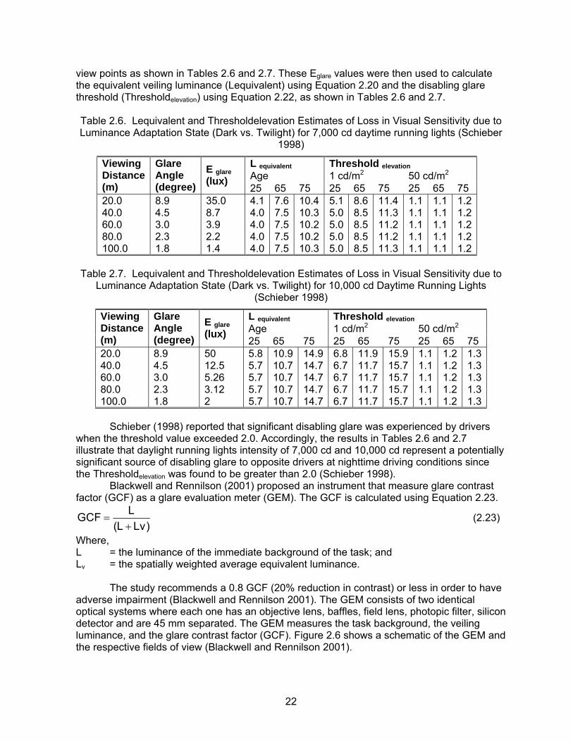
22
view points as shown in Tables 2.6 and 2.7. These Eglare values were then used to calculate the equivalent veiling luminance (Lequivalent) using Equation 2.20 and the disabling glare threshold (Thresholdelevation) using Equation 2.22, as shown in Tables 2.6 and 2.7. Table 2.6. Lequivalent and Thresholdelevation Estimates of Loss in Visual Sensitivity due to Luminance Adaptation State (Dark vs. Twilight) for 7,000 cd daytime running lights (Schieber
1998)
L equivalent Threshold elevation Age 1 cd/m2 50 cd/m2
Viewing Distance (m)
Glare Angle (degree)
E glare (lux)
25 65 75 25 65 75 25 65 75 20.0 8.9 35.0 4.1 7.6 10.4 5.1 8.6 11.4 1.1 1.1 1.240.0 4.5 8.7 4.0 7.5 10.3 5.0 8.5 11.3 1.1 1.1 1.260.0 3.0 3.9 4.0 7.5 10.2 5.0 8.5 11.2 1.1 1.1 1.280.0 2.3 2.2 4.0 7.5 10.2 5.0 8.5 11.2 1.1 1.1 1.2100.0 1.8 1.4 4.0 7.5 10.3 5.0 8.5 11.3 1.1 1.1 1.2
Table 2.7. Lequivalent and Thresholdelevation Estimates of Loss in Visual Sensitivity due to
Luminance Adaptation State (Dark vs. Twilight) for 10,000 cd Daytime Running Lights (Schieber 1998)
L equivalent Threshold elevation Age 1 cd/m2 50 cd/m2
Viewing Distance (m)
Glare Angle (degree)
E glare (lux)
25 65 75 25 65 75 25 65 75 20.0 8.9 50 5.8 10.9 14.9 6.8 11.9 15.9 1.1 1.2 1.340.0 4.5 12.5 5.7 10.7 14.7 6.7 11.7 15.7 1.1 1.2 1.360.0 3.0 5.26 5.7 10.7 14.7 6.7 11.7 15.7 1.1 1.2 1.380.0 2.3 3.12 5.7 10.7 14.7 6.7 11.7 15.7 1.1 1.2 1.3100.0 1.8 2 5.7 10.7 14.7 6.7 11.7 15.7 1.1 1.2 1.3
Schieber (1998) reported that significant disabling glare was experienced by drivers when the threshold value exceeded 2.0. Accordingly, the results in Tables 2.6 and 2.7 illustrate that daylight running lights intensity of 7,000 cd and 10,000 cd represent a potentially significant source of disabling glare to opposite drivers at nighttime driving conditions since the Thresholdelevation was found to be greater than 2.0 (Schieber 1998). Blackwell and Rennilson (2001) proposed an instrument that measure glare contrast factor (GCF) as a glare evaluation meter (GEM). The GCF is calculated using Equation 2.23.
)LvL(LGCF+
= (2.23)
Where, L = the luminance of the immediate background of the task; and Lv = the spatially weighted average equivalent luminance. The study recommends a 0.8 GCF (20% reduction in contrast) or less in order to have adverse impairment (Blackwell and Rennilson 2001). The GEM consists of two identical optical systems where each one has an objective lens, baffles, field lens, photopic filter, silicon detector and are 45 mm separated. The GEM measures the task background, the veiling luminance, and the glare contrast factor (GCF). Figure 2.6 shows a schematic of the GEM and the respective fields of view (Blackwell and Rennilson 2001).

23
Figure 2.6. Schematic view of the GEM and the respective fields of view (Blackwell and
Rennilson 2001).
2.4.3. Pavement Luminance Measurement To determine pavement luminance, site measurements can be made using a luminance meter at various possible observer points in the field of view to estimate an average value for this parameter. However, luminance meters are expensive, which may limit their availability and use in the design of nighttime construction sites. In addition, these measurements are rarely made prior to the design of lighting arrangements. As an alternative solution, pavement luminance can be calculated based on a two-dimensional array of light reflection coefficients referred to as the r-tables. In recent years, however, research studies have raised concerns about the accuracy of this procedure and whether adopted reflection coefficients are applicable to new generations of pavement materials such as open-graded friction course and to predominant pavement conditions (Khan et al. 1999). The measurement of pavement luminance is based on identifying a representative average value that considers various possible view points according to the following four main steps (these steps can be repeated at any desired observer position (p)): (1). Identify a set of all possible view points (g = 1 to G) that exist in the field of view of the
driver. These points are set to be equally spaced and cover the field of view at a distance of 83m ahead of the considered observer position p as shown in Figure 2.7. This distance was set by the Illuminating Engineering Society of North America (IESNA) standards for roadway lighting, which set the line of sight of the driver to be inclined 1o downward, and the average height of the driver’s eye assumed 1.45m (IESNA 2000). Although not considered in the IESNA specifications, this viewing angle would be greater than 1o for drivers of trucks, buses, vans, and SUVs while the viewing angle will be smaller than this value for drivers of sport cars.
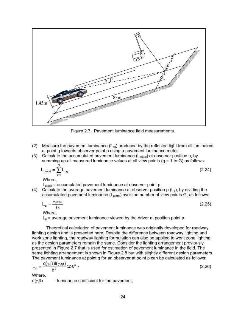
24
Figure 2.7. Pavement luminance field measurements.
(2). Measure the pavement luminance (Lpg) produced by the reflected light from all luminaires at point g towards observer point p using a pavement luminance meter.
(3). Calculate the accumulated pavement luminance (Lptotal) at observer position p, by summing up all measured luminance values at all view points (g = 1 to G) as follows:
∑=
=G
1gpgptotal LL (2.24)
Where, Lptotal = accumulated pavement luminance at observer point p.
(4). Calculate the average pavement luminance at observer position p (Lp), by dividing the accumulated pavement luminance (Lptotal) over the number of view points G, as follows:
G
LL ptotal
p = (2.25)
Where, Lp = average pavement luminance viewed by the driver at position point p.
Theoretical calculation of pavement luminance was originally developed for roadway lighting design and is presented here. Despite the difference between roadway lighting and work zone lighting, the roadway lighting formulation can also be applied to work zone lighting as the design parameters remain the same. Consider the lighting arrangement previously presented in Figure 2.7 that is used for estimation of pavement luminance in the field. The same lighting arrangement is shown in Figure 2.8 but with slightly different design parameters. The pavement luminance at point g for an observer at point p can be calculated as follows:
γϕγβγ
= 32p cos
h),(I),(qL (2.26)
Where, q(γ,β) = luminance coefficient for the pavement;
g
1o
83m1.45m
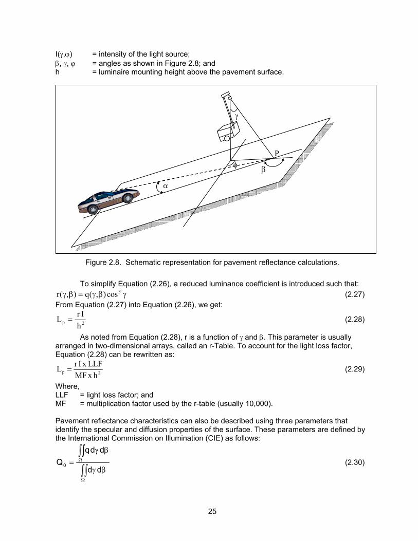
25
I(γ,ϕ) = intensity of the light source; β, γ, ϕ = angles as shown in Figure 2.8; and h = luminaire mounting height above the pavement surface.
Figure 2.8. Schematic representation for pavement reflectance calculations.
To simplify Equation (2.26), a reduced luminance coefficient is introduced such that:
γβγ=βγ 3cos),(q),(r (2.27) From Equation (2.27) into Equation (2.26), we get:
2p hIrL = (2.28)
As noted from Equation (2.28), r is a function of γ and β. This parameter is usually arranged in two-dimensional arrays, called an r-Table. To account for the light loss factor, Equation (2.28) can be rewritten as:
2p hxMFLLFxIrL = (2.29)
Where, LLF = light loss factor; and MF = multiplication factor used by the r-table (usually 10,000). Pavement reflectance characteristics can also be described using three parameters that identify the specular and diffusion properties of the surface. These parameters are defined by the International Commission on Illumination (CIE) as follows:
∫∫
∫∫
Ω
Ω
βγ
βγ=
dd
ddqQ0 (2.30)
P
α
β
γ
φ
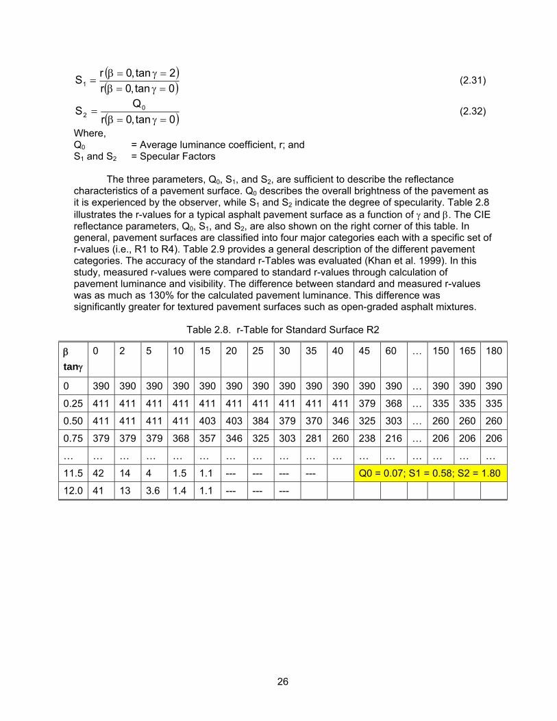
26
( )( )0tan,0r
2tan,0rS1 =γ=β=γ=β
= (2.31)
( )0tan,0rQ
S 02 =γ=β= (2.32)
Where, Q0 = Average luminance coefficient, r; and S1 and S2 = Specular Factors The three parameters, Q0, S1, and S2, are sufficient to describe the reflectance characteristics of a pavement surface. Q0 describes the overall brightness of the pavement as it is experienced by the observer, while S1 and S2 indicate the degree of specularity. Table 2.8 illustrates the r-values for a typical asphalt pavement surface as a function of γ and β. The CIE reflectance parameters, Q0, S1, and S2, are also shown on the right corner of this table. In general, pavement surfaces are classified into four major categories each with a specific set of r-values (i.e., R1 to R4). Table 2.9 provides a general description of the different pavement categories. The accuracy of the standard r-Tables was evaluated (Khan et al. 1999). In this study, measured r-values were compared to standard r-values through calculation of pavement luminance and visibility. The difference between standard and measured r-values was as much as 130% for the calculated pavement luminance. This difference was significantly greater for textured pavement surfaces such as open-graded asphalt mixtures.
Table 2.8. r-Table for Standard Surface R2
β tanγ
0 2 5 10 15 20 25 30 35 40 45 60 … 150 165 180
0 390 390 390 390 390 390 390 390 390 390 390 390 … 390 390 390
0.25 411 411 411 411 411 411 411 411 411 411 379 368 … 335 335 335
0.50 411 411 411 411 403 403 384 379 370 346 325 303 … 260 260 260
0.75 379 379 379 368 357 346 325 303 281 260 238 216 … 206 206 206
… … … … … … … … … … … … … … … … …
11.5 42 14 4 1.5 1.1 --- --- --- --- Q0 = 0.07; S1 = 0.58; S2 = 1.80
12.0 41 13 3.6 1.4 1.1 --- --- ---

27
Table 2.9. Pavement Categories and Their Characteristics (IESNA 2000)
Class Description Mode of reflectance R1 Portland cement concrete road surface. Asphalt
road with a minimum of 15% of the artificial brightener (e.g., Synopal) aggregate (e.g., labradorite, quartzite).
Mostly diffuse
R2 Asphalt road surface with an aggregate composed of a minimum 60% gravel (size greater than 10mm)
Mixed (diffuse and specular)
R3 Asphalt road surface (regular and carpet seal) with dark aggregates (e.g., trap rock, blast furnace slag); rough texture after some months of use (typical highways)
Slightly specular
R4 Asphalt road with very smooth texture Mostly specular Both Q0 and S1 can be measured using a Portable Road Surface Reflectometer. Table 2.10 shows the CIE reflectance parameters for the four pavement categories. If the measured Q0 differs from the standard values shown in Table 2.10, all reflectance coefficients, r, need to be adjust proportionally (Jung et al. 1984).
Table 2.10. Reflectance Parameters for the Four Pavement Categories
R Series Parameter
R1 R2 R3 R4
Q0 0.10 0.07 0.07 0.08
S1 0.25 0.58 1.11 1.55
S2 1.53 1.80 2.38 3.03 Research has also shown that pavement reflectance varies significantly with traffic wear and the location with respect to the wheel path (Khan et al. 1999). This is particularly critical with asphalt surfaces, which show increased brightness and specularity with aging and deterioration. As a result, pavement reflectance may vary significantly in the same pavement depending on the locations (in or away from the wheel path), climatic conditions (wet or dry), aging and deterioration. Research also indicates that fine-grained mixtures exhibit greater variation in pavement reflectance than coarse-grained mixtures. In fine-grained mixtures, it appears that the effect of surface depressions is more pronounced than in coarse-grained mixtures (Bassett et al. 1988). In these cases, assuming only one standard r-table for a particular pavement type may result in erroneous calculations of the pavement luminance due to the large discrepancies that may exist in the same road section. To investigate the effects of pavement characteristics on the measured luminance and to develop accurate classification criteria, a limited number of studies used a laboratory measurement setup (Jung et al. 1984; King and Finch 1978). In one of the most notable laboratory setups, a sample obtained from a pavement core is placed horizontally on a rotating table, and is illuminated from various positions defined by angle γ. A photometer is then used to measure the reflected light at a viewing angle α of 1o. The sample and the fixed photometer rotate around the axis X-X to simulate the rotating angle β ranging from 0 to 180o. Figure 2.8 illustrates the described laboratory experimental setup and Figure 2.9 shows the corresponding field setup with the same design parameters. Using this setup, reduced

28
luminance coefficients, r(β, tanγ), can be estimated for different lighting conditions as defined by the angles β, and γ. Using the described laboratory test setup, an r-table can be obtained for each pavement sample by varying the angle β and tanγ from 0 to 180o and from 0 to 12, respectively. Each coefficient, r, is calculated as follows:
ILhr
2
= (2.33)
Where, L = measured pavement luminance in cd/m2; h = height of lamp above the sample surface (set in this setup at 0.68m); and I = luminous intensity of the lamp, in lumens.
Figure 2.9. Laboratory setup utilized by Jung et al. (1984).
It was reported that on the same pavement sample, the variability of the developed laboratory setup was no greater than 2%. A critical factor that was also discussed in this study includes the influence of the measurement location on the road on the accuracy. As previously mentioned, pavement reflectance varies significantly with the measurement location with respect to the wheel path and depending on the differences in pavement wear, mixture compaction, contamination of the pavement surface, and segregation of the mixture. It was found that measurements of pavement reflection along the wheel path of a newly-constructed road section varied by a percentage ranging between 6% and 20%. On the other hand, measurements over the whole road section varied by a percentage ranging between 2% and 56%. Pavement reflectance is also influenced by the degree of wetness of the surface, which in turn affects the lighting and safety conditions of the roadway. Using a laboratory test setup similar to the one shown in Figure 2.9, the influence of pavement wetness was evaluated (Bassett et al. 1988). In this study, a dry pavement sample was sprayed with a mist of water until saturated, and the drying surface reflectance characteristics were monitored over time. To maintain a desired level of saturation through measurements needed to develop an r-table, a closed loop system allowing the control of the mist of water was used. Unfortunately, results of this study did not directly quantify the effect of pavement wetness on the reflectance characteristics of a given surface. However, for the coarse-grained samples, a 10 minute drying time resulted in a 23% decrease in the average reflectance coefficient Q0 indicating that wet surfaces are characterized by a greater brightness than dry surface. For
Luminaire
X
Photometer
X
Sample
1o γ h=0.68m
29
the fine-grained samples, a 10-minute drying time resulted in a 144% decrease in Q0 indicating their strong dependency on the level of saturation at the surface.
2.5. Available Standards and Recommendations The following three sections highlight: (1) existing glare recommendations by several USDOTs; (2) existing glare recommendations by professional organizations; and (3) existing guidelines and hardware for glare control.
2.5.1. U.S. Departments of Transportation Several U.S. Departments of Transportation have developed recommendations to control glare caused by nighttime highway lighting. This section provides a review of the existing recommendations that were obtained in this literature review from nine states: Virginia, New York, California, Tennessee, Indiana, South Carolina, Delaware, Florida, and Oregon. 2.5.1.1. Virginia The Virginia Department of Transportation (VDOT) recommends that temporary lighting for night work should be designed so that glare does not interfere with driver’s visibility or create visibility problems for truck drivers, equipment operators, flaggers, or other workers. The adequacy of the floodlight placement and elimination of potential glare shall be determined by driving through and observing the floodlighted area from each direction on all approaching roadways after the initial floodlight setup, and periodically during each shift (VDOT 2005). Moreover, the use of screens mounted on the top of temporary traffic barriers should be considered in crossover applications whenever multi-lane traffic is reduced to two-way motor vehicle traffic to reduce headlight glare from oncoming traffic and improve mobility through the crossover (VDOT 2005). 2.5.1.2. New York The New York Department of Transportation (NYDOT) provides a number of requirements that need to be met to avoid objectionable levels of glare, including (1) all luminaires should be aimed so that the center of the beam axis is not greater than 60 degrees from the vertical; (2) no luminaires that provide luminance intensity greater than 20,000 candelas at an angle 72 degree above the vertical should be permitted; (3) the contractor should be responsible for providing shields, visors, or louvers on luminaires when necessary to reduce objectionable levels of glare (NYDOT 1995). 2.5.1.3. California The California Department of Transportation (Caltrans) suggests using glare screens in order to control harmful glare from the opposite traffic. The glare screen should be installed only on barriers where the median is 6.1 m or less. Moreover, Caltrans requires contractors to control glare in nighttime highway construction by directing the light onto the construction area and to avoid shining lights toward residences (California DOT 2001). 2.5.1.4. Tennessee The Tennessee Department of Transportation (TDOT) recommends that all luminaries in nighttime highway construction be located and directed in such a way to minimize glare to both motorists and work vehicles. If glare is noted from any travel path, the contractor must adjust the lighting to reduce the glare to an acceptable level to the satisfaction of the Engineer (TDOT 2006).
30
2.5.1.5. Indiana The Indiana Department of Transportation (INDOT) recommends the use of glare screens to control objectionable glare in nighttime highway construction. Typical applications of glare screens in construction zones are at crossover transitions and in 2-way, 2-lane operations (INDOT 2006). 2.5.1.6. South Carolina The South Carolina Department of Transportation (SCDOT) recommends that the contractor furnish, place, and maintain lighting facilities to provide light of sufficient intensity to facilitate good workmanship and proper inspection in all areas where work is being performed during the hours of darkness. SCDOT also recommends that lighting shall be arranged so as not to produce glare or diminish the motorist’s visibility (SCDOT 2000). 2.5.1.7. Delaware The Delaware Department of Transportation (DelDOT) recommends the use of floodlights to light work activities, flagger stations and other restricted or hazardous areas at night when area lighting is not sufficient. DelDOT also requires that floodlights be positioned or shielded to prevent glare to drivers (DelDOT 2001). 2.5.1.8. Florida The Florida DOT recommends the use of glare screens as a mean for controlling glare. The screen has to be added temporarily to barriers on locations identified on the construction plans. 2.5.1.9. Oregon The Oregon Department of Transportation (ODOT) recommends using glare shields suitable for placement on the top of concrete median barrier to block vehicle headlights from blinding on-coming motorists (ODOT 2001). Other U.S. DOT recommend applying screens or barrier walls to shield workers, adjacent properties, and traveling public from objectionable glare. Table 2.11 shows an example of some states that use screens and barriers to avoid glare (Amos 1994).
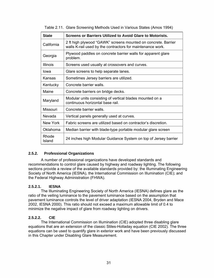
31
Table 2.11. Glare Screening Methods Used in Various States (Amos 1994)
State Screens or Barriers Utilized to Avoid Glare to Motorists.
California 2 ft high plywood “GAWK” screens mounted on concrete. Barrier walls K-rail used by the contractors for maintenance work.
Georgia Plywood paddles on concrete barrier walls for apparent glare problem.
Illinois Screens used usually at crossovers and curves.
Iowa Glare screens to help separate lanes.
Kansas Sometimes Jersey barriers are utilized.
Kentucky Concrete barrier walls.
Maine Concrete barriers on bridge decks.
Maryland Modular units consisting of vertical blades mounted on a continuous horizontal base rail.
Missouri Concrete barrier walls.
Nevada Vertical panels generally used at curves.
New York Fabric screens are utilized based on contractor’s discretion.
Oklahoma Median barrier with blade-type portable modular glare screen
Rhode Island 24 inches high Modular Guidance System on top of Jersey barrier
2.5.2. Professional Organizations A number of professional organizations have developed standards and recommendations to control glare caused by highway and roadway lighting. The following sections provide a review of the available standards provided by: the Illuminating Engineering Society of North America (IESNA), the International Commission on Illumination (CIE); and the Federal Highway Administration (FHWA). 2.5.2.1. IESNA The Illuminating Engineering Society of North America (IESNA) defines glare as the ratio of the veiling luminance to the pavement luminance based on the assumption that pavement luminance controls the level of driver adaptation (IESNA 2004, Bryden and Mace 2002, IESNA 2000). This ratio should not exceed a maximum allowable limit of 0.4 to minimize the negative impact of glare from roadway lighting on drivers. 2.5.2.2. CIE The International Commission on Illumination (CIE) adopted three disabling glare equations that are an extension of the classic Stiles-Holladay equation (CIE 2002). The three equations can be used to quantify glare in exterior work and have been previously discussed in this Chapter under Disabling Glare Measurement.
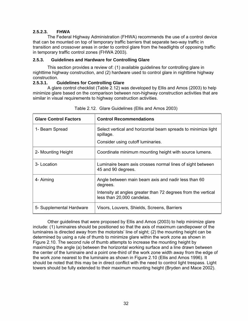
32
2.5.2.3. FHWA The Federal Highway Administration (FHWA) recommends the use of a control device that can be mounted on top of temporary traffic barriers that separate two-way traffic in transition and crossover areas in order to control glare from the headlights of opposing traffic in temporary traffic control zones (FHWA 2003).
2.5.3. Guidelines and Hardware for Controlling Glare This section provides a review of: (1) available guidelines for controlling glare in nighttime highway construction, and (2) hardware used to control glare in nighttime highway construction. 2.5.3.1. Guidelines for Controlling Glare A glare control checklist (Table 2.12) was developed by Ellis and Amos (2003) to help minimize glare based on the comparison between non-highway construction activities that are similar in visual requirements to highway construction activities.
Table 2.12. Glare Guidelines (Ellis and Amos 2003)
Glare Control Factors Control Recommendations
1- Beam Spread Select vertical and horizontal beam spreads to minimize light spillage.
Consider using cutoff luminaries.
2- Mounting Height Coordinate minimum mounting height with source lumens.
3- Location Luminaire beam axis crosses normal lines of sight between 45 and 90 degrees.
4- Aiming Angle between main beam axis and nadir less than 60 degrees.
Intensity at angles greater than 72 degrees from the vertical less than 20,000 candelas.
5- Supplemental Hardware Visors, Louvers, Shields, Screens, Barriers
Other guidelines that were proposed by Ellis and Amos (2003) to help minimize glare include: (1) luminaires should be positioned so that the axis of maximum candlepower of the luminaires is directed away from the motorists’ line of sight; (2) the mounting height can be determined by using a rule of thumb to minimize glare within the work zone as shown in Figure 2.10. The second rule of thumb attempts to increase the mounting height by maximizing the angle (a) between the horizontal working surface and a line drawn between the center of the luminaire and a point one-third of the work zone width away from the edge of the work zone nearest to the luminaire as shown in Figure 2.10 (Ellis and Amos 1996). It should be noted that this may be in direct conflict with the need to control light trespass. Light towers should be fully extended to their maximum mounting height (Bryden and Mace 2002).
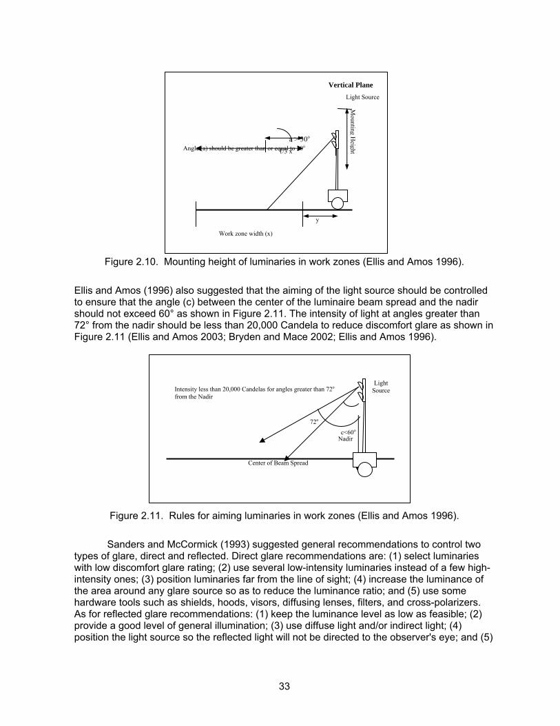
33
Figure 2.10. Mounting height of luminaries in work zones (Ellis and Amos 1996).
Ellis and Amos (1996) also suggested that the aiming of the light source should be controlled to ensure that the angle (c) between the center of the luminaire beam spread and the nadir should not exceed 60° as shown in Figure 2.11. The intensity of light at angles greater than 72° from the nadir should be less than 20,000 Candela to reduce discomfort glare as shown in Figure 2.11 (Ellis and Amos 2003; Bryden and Mace 2002; Ellis and Amos 1996).
Figure 2.11. Rules for aiming luminaries in work zones (Ellis and Amos 1996).
Sanders and McCormick (1993) suggested general recommendations to control two types of glare, direct and reflected. Direct glare recommendations are: (1) select luminaries with low discomfort glare rating; (2) use several low-intensity luminaries instead of a few high-intensity ones; (3) position luminaries far from the line of sight; (4) increase the luminance of the area around any glare source so as to reduce the luminance ratio; and (5) use some hardware tools such as shields, hoods, visors, diffusing lenses, filters, and cross-polarizers. As for reflected glare recommendations: (1) keep the luminance level as low as feasible; (2) provide a good level of general illumination; (3) use diffuse light and/or indirect light; (4) position the light source so the reflected light will not be directed to the observer's eye; and (5)
a > 30o
c<60o
Intensity less than 20,000 Candelas for angles greater than 72o from the Nadir
Nadir
Light Source
Center of Beam Spread
1/3 x
Mounting H
eight
Light Source
72o
y
Work zone width (x)
Angle (a) should be greater than or equal to 30o
Vertical Plane
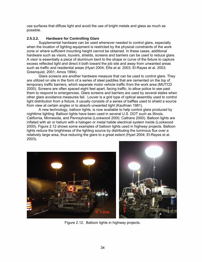
34
use surfaces that diffuse light and avoid the use of bright metals and glass as much as possible. 2.5.3.2. Hardware for Controlling Glare Supplemental hardware can be used whenever needed to control glare, especially when the location of lighting equipment is restricted by the physical constraints of the work zone or where sufficient mounting height cannot be obtained. In these cases, additional hardware such as visors, louvers, shields, screens and barriers can be used to reduce glare. A visor is essentially a piece of aluminum bent to the shape or curve of the fixture to capture excess reflected light and direct it both toward the job site and away from unwanted areas such as traffic and residential areas (Hyari 2004; Ellis et al. 2003; El-Rayes et al. 2003; Greenquist, 2001; Amos 1994). Glare screens are another hardware measure that can be used to control glare. They are utilized on site in the form of a series of steel paddles that are cemented on the top of temporary traffic barriers, which separate motor vehicle traffic from the work area (MUTCD 2000). Screens are often spaced eight feet apart, facing traffic, to allow police to see past them to respond to emergencies. Glare screens and barriers are used by several states when other glare avoidance measures fail. Louver is a grid type of optical assembly used to control light distribution from a fixture, it usually consists of a series of baffles used to shield a source from view at certain angles or to absorb unwanted light (Kaufman 1981). A new technology, balloon lights, is now available to help control glare produced by nighttime lighting. Balloon lights have been used in several U.S. DOT such as Illinois, California, Minnesota, and Pennsylvania (Lockwood 2000, Caltrans 2000). Balloon lights are inflated with air or helium with a halogen or metal halide electrical system inside (Lockwood 2000). Figure 2.12 shows some examples of balloon lights used in highway projects. Balloon lights reduce the brightness of the lighting source by distributing the luminous flux over a relatively large area, thus reducing the glare to a great extent (Hyari 2004; El-Rayes et al. 2003).
Figure 2.12. Balloon lights in highway projects.
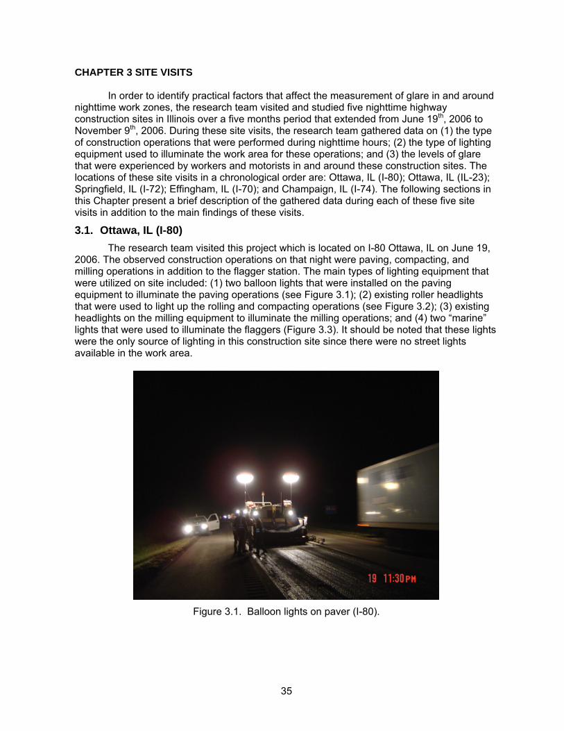
35
CHAPTER 3 SITE VISITS 3. 5 In order to identify practical factors that affect the measurement of glare in and around nighttime work zones, the research team visited and studied five nighttime highway construction sites in Illinois over a five months period that extended from June 19th, 2006 to November 9th, 2006. During these site visits, the research team gathered data on (1) the type of construction operations that were performed during nighttime hours; (2) the type of lighting equipment used to illuminate the work area for these operations; and (3) the levels of glare that were experienced by workers and motorists in and around these construction sites. The locations of these site visits in a chronological order are: Ottawa, IL (I-80); Ottawa, IL (IL-23); Springfield, IL (I-72); Effingham, IL (I-70); and Champaign, IL (I-74). The following sections in this Chapter present a brief description of the gathered data during each of these five site visits in addition to the main findings of these visits.
3.1. Ottawa, IL (I-80) The research team visited this project which is located on I-80 Ottawa, IL on June 19, 2006. The observed construction operations on that night were paving, compacting, and milling operations in addition to the flagger station. The main types of lighting equipment that were utilized on site included: (1) two balloon lights that were installed on the paving equipment to illuminate the paving operations (see Figure 3.1); (2) existing roller headlights that were used to light up the rolling and compacting operations (see Figure 3.2); (3) existing headlights on the milling equipment to illuminate the milling operations; and (4) two “marine” lights that were used to illuminate the flaggers (Figure 3.3). It should be noted that these lights were the only source of lighting in this construction site since there were no street lights available in the work area.
Figure 3.1. Balloon lights on paver (I-80).
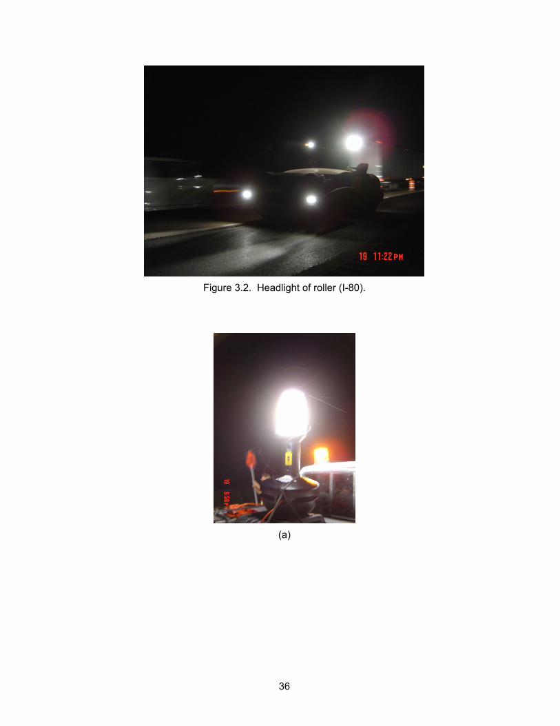
36
Figure 3.2. Headlight of roller (I-80).
(a)
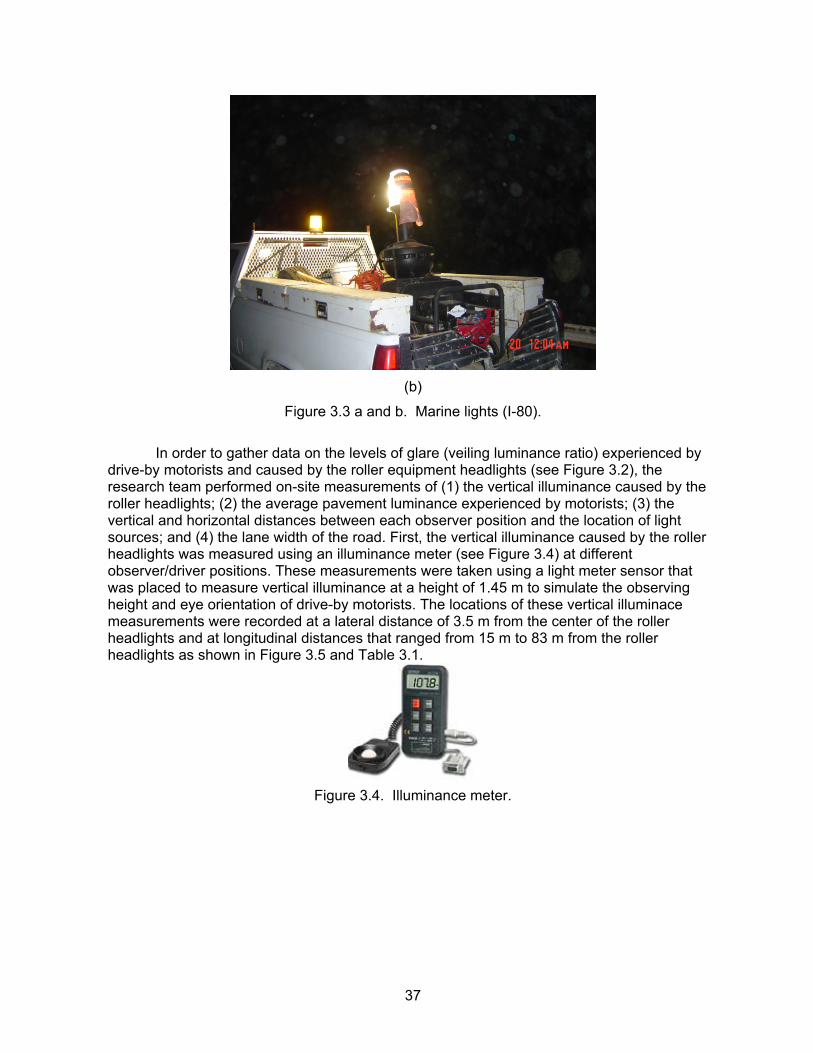
37
(b)
Figure 3.3 a and b. Marine lights (I-80).
In order to gather data on the levels of glare (veiling luminance ratio) experienced by drive-by motorists and caused by the roller equipment headlights (see Figure 3.2), the research team performed on-site measurements of (1) the vertical illuminance caused by the roller headlights; (2) the average pavement luminance experienced by motorists; (3) the vertical and horizontal distances between each observer position and the location of light sources; and (4) the lane width of the road. First, the vertical illuminance caused by the roller headlights was measured using an illuminance meter (see Figure 3.4) at different observer/driver positions. These measurements were taken using a light meter sensor that was placed to measure vertical illuminance at a height of 1.45 m to simulate the observing height and eye orientation of drive-by motorists. The locations of these vertical illuminace measurements were recorded at a lateral distance of 3.5 m from the center of the roller headlights and at longitudinal distances that ranged from 15 m to 83 m from the roller headlights as shown in Figure 3.5 and Table 3.1.
Figure 3.4. Illuminance meter.
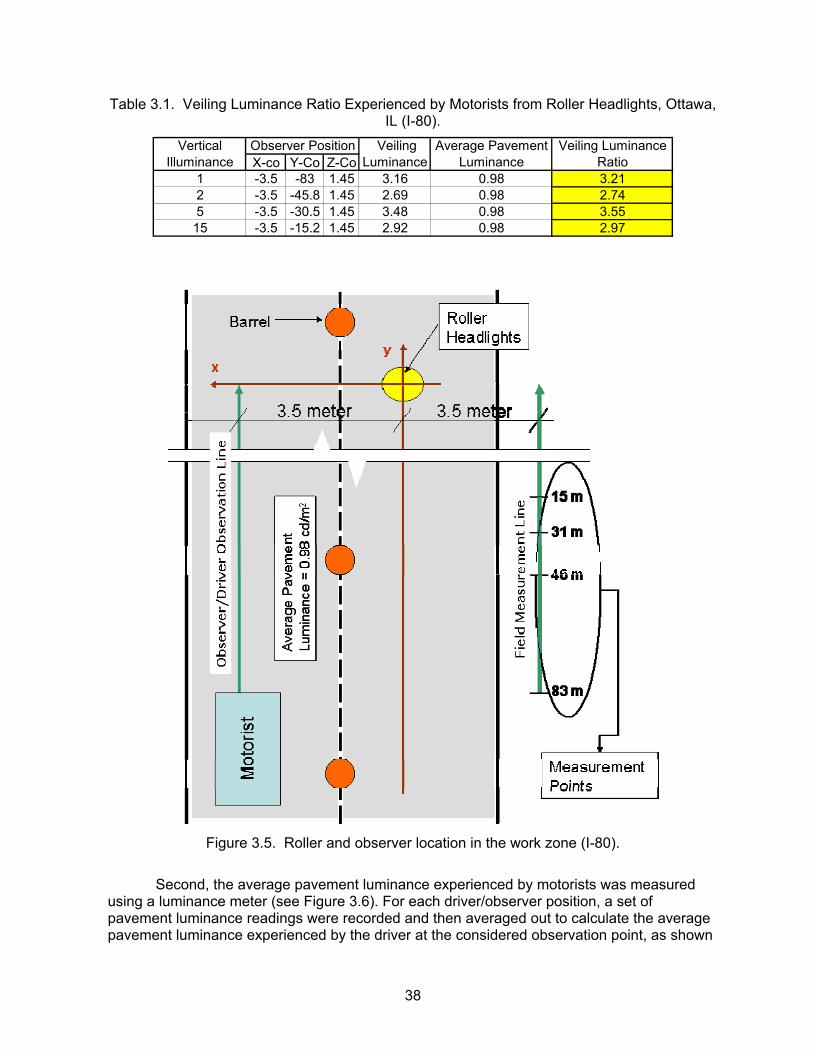
38
Table 3.1. Veiling Luminance Ratio Experienced by Motorists from Roller Headlights, Ottawa, IL (I-80).
X-co Y-Co Z-Co1 -3.5 -83 1.45 3.16 0.98 3.212 -3.5 -45.8 1.45 2.69 0.98 2.745 -3.5 -30.5 1.45 3.48 0.98 3.5515 -3.5 -15.2 1.45 2.92 0.98 2.97
Vertical Illuminance
Observer Position Veiling Luminance Ratio
Veiling Luminance
Average Pavement Luminance
Figure 3.5. Roller and observer location in the work zone (I-80).
Second, the average pavement luminance experienced by motorists was measured
using a luminance meter (see Figure 3.6). For each driver/observer position, a set of pavement luminance readings were recorded and then averaged out to calculate the average pavement luminance experienced by the driver at the considered observation point, as shown
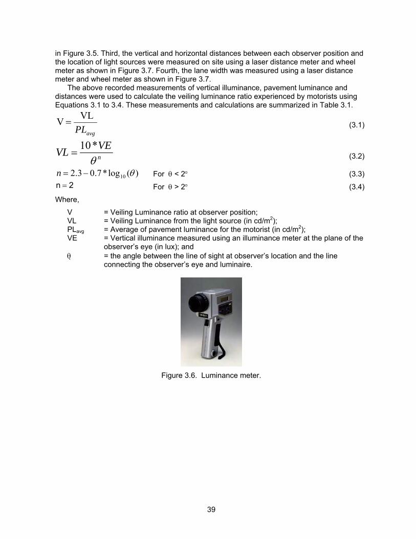
39
in Figure 3.5. Third, the vertical and horizontal distances between each observer position and the location of light sources were measured on site using a laser distance meter and wheel meter as shown in Figure 3.7. Fourth, the lane width was measured using a laser distance meter and wheel meter as shown in Figure 3.7. The above recorded measurements of vertical illuminance, pavement luminance and distances were used to calculate the veiling luminance ratio experienced by motorists using Equations 3.1 to 3.4. These measurements and calculations are summarized in Table 3.1.
avgPLVL V = (3.1)
nVEVL
θ*10
= (3.2)
)(log*7.03.2 10 θ−=n For θ < 2° (3.3) 2n = For θ > 2° (3.4)
Where,
V = Veiling Luminance ratio at observer position; VL = Veiling Luminance from the light source (in cd/m2); PLavg = Average of pavement luminance for the motorist (in cd/m2); VE = Vertical illuminance measured using an illuminance meter at the plane of the
observer’s eye (in lux); and θ = the angle between the line of sight at observer’s location and the line
connecting the observer’s eye and luminaire.
Figure 3.6. Luminance meter.
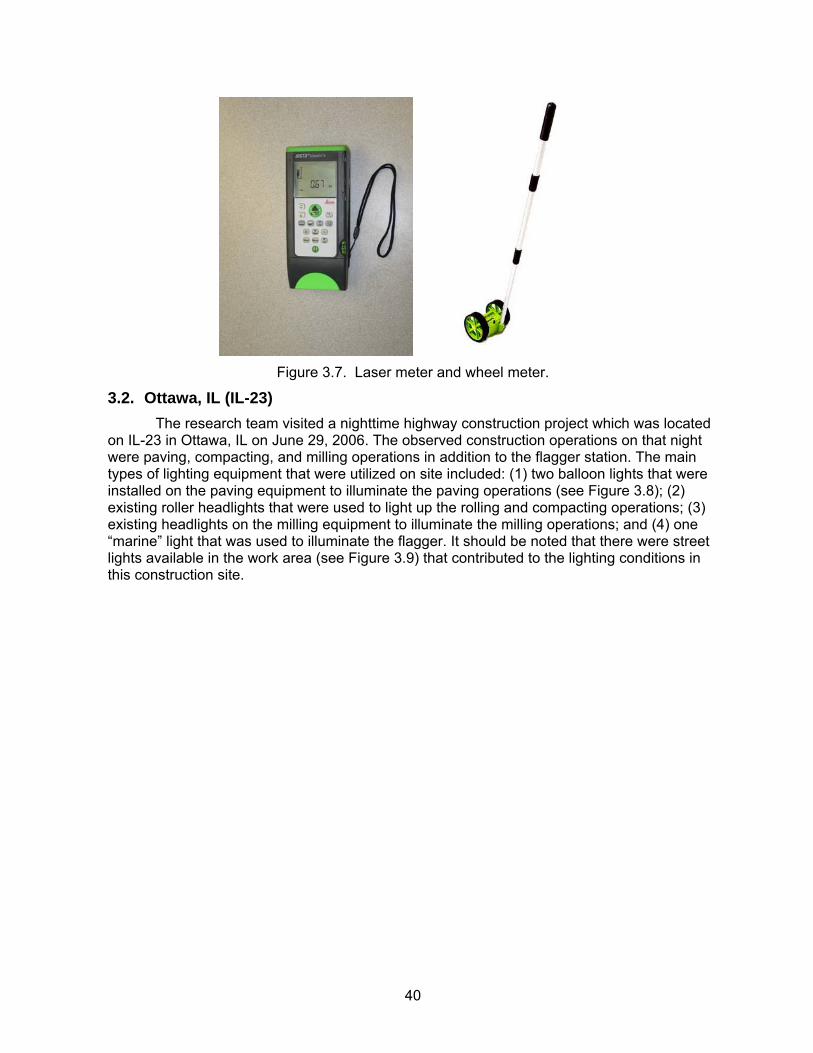
40
Figure 3.7. Laser meter and wheel meter.
3.2. Ottawa, IL (IL-23) The research team visited a nighttime highway construction project which was located on IL-23 in Ottawa, IL on June 29, 2006. The observed construction operations on that night were paving, compacting, and milling operations in addition to the flagger station. The main types of lighting equipment that were utilized on site included: (1) two balloon lights that were installed on the paving equipment to illuminate the paving operations (see Figure 3.8); (2) existing roller headlights that were used to light up the rolling and compacting operations; (3) existing headlights on the milling equipment to illuminate the milling operations; and (4) one “marine” light that was used to illuminate the flagger. It should be noted that there were street lights available in the work area (see Figure 3.9) that contributed to the lighting conditions in this construction site.

41
Figure 3.8. Balloon lights on paver (IL-23).
Figure 3.9. Street lights (IL-23).
The research performed on-site measurements to calculate the levels of glare (veiling luminance ratio) experienced by drive-by motorists and caused by the two balloon lights that
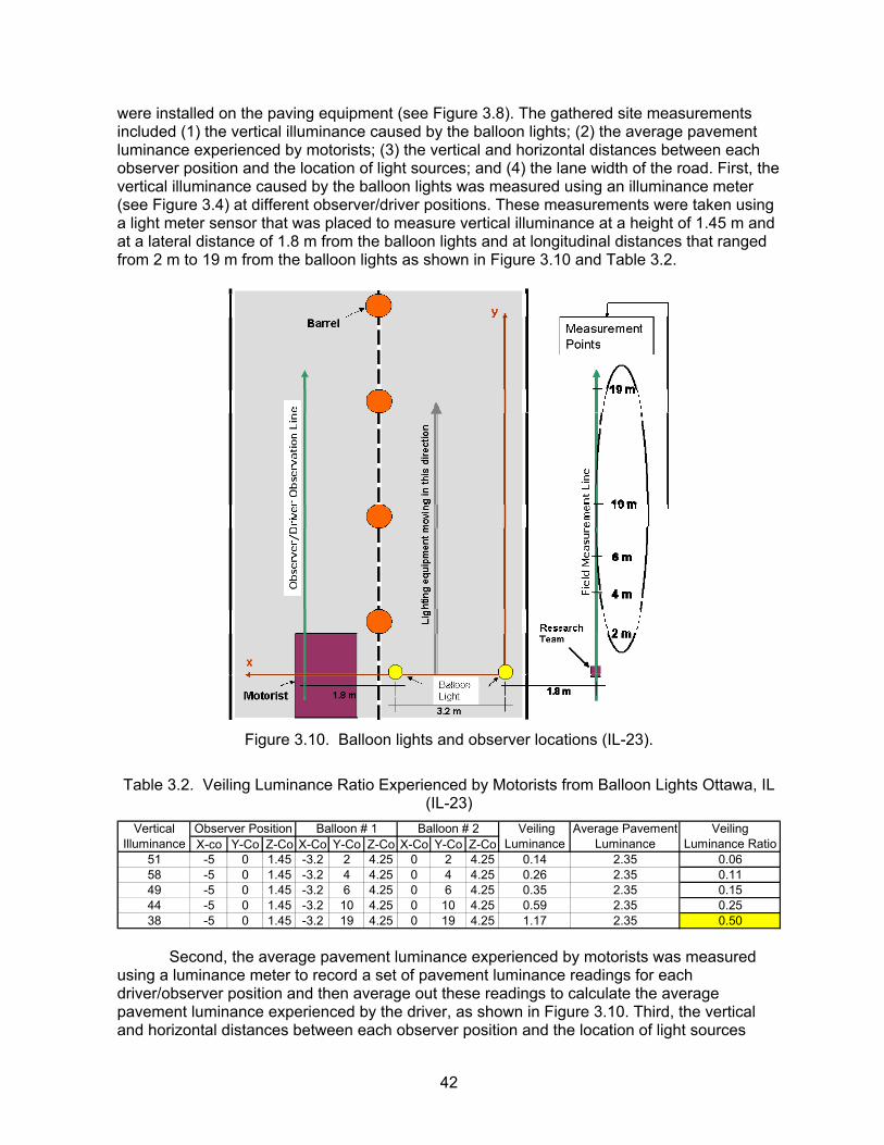
42
were installed on the paving equipment (see Figure 3.8). The gathered site measurements included (1) the vertical illuminance caused by the balloon lights; (2) the average pavement luminance experienced by motorists; (3) the vertical and horizontal distances between each observer position and the location of light sources; and (4) the lane width of the road. First, the vertical illuminance caused by the balloon lights was measured using an illuminance meter (see Figure 3.4) at different observer/driver positions. These measurements were taken using a light meter sensor that was placed to measure vertical illuminance at a height of 1.45 m and at a lateral distance of 1.8 m from the balloon lights and at longitudinal distances that ranged from 2 m to 19 m from the balloon lights as shown in Figure 3.10 and Table 3.2.
Figure 3.10. Balloon lights and observer locations (IL-23).
Table 3.2. Veiling Luminance Ratio Experienced by Motorists from Balloon Lights Ottawa, IL
(IL-23)
X-co Y-Co Z-Co X-Co Y-Co Z-Co X-Co Y-Co Z-Co51 -5 0 1.45 -3.2 2 4.25 0 2 4.25 0.14 2.35 0.0658 -5 0 1.45 -3.2 4 4.25 0 4 4.25 0.26 2.35 0.1149 -5 0 1.45 -3.2 6 4.25 0 6 4.25 0.35 2.35 0.1544 -5 0 1.45 -3.2 10 4.25 0 10 4.25 0.59 2.35 0.2538 -5 0 1.45 -3.2 19 4.25 0 19 4.25 1.17 2.35 0.50
Balloon # 1 Balloon # 2 Veiling Luminance Ratio
Veiling Luminance
Average Pavement Luminance
Vertical Illuminance
Observer Position
Second, the average pavement luminance experienced by motorists was measured using a luminance meter to record a set of pavement luminance readings for each driver/observer position and then average out these readings to calculate the average pavement luminance experienced by the driver, as shown in Figure 3.10. Third, the vertical and horizontal distances between each observer position and the location of light sources
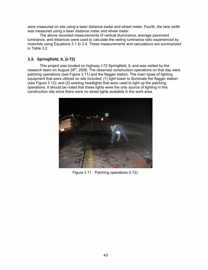
43
were measured on site using a laser distance meter and wheel meter. Fourth, the lane width was measured using a laser distance meter and wheel meter. The above recorded measurements of vertical illuminance, average pavement luminance, and distances were used to calculate the veiling luminance ratio experienced by motorists using Equations 3.1 to 3.4. These measurements and calculations are summarized in Table 3.2.
3.3. Springfield, IL (I-72) This project was located on highway I-72 Springfield, IL and was visited by the research team on August 28th, 2006. The observed construction operations on that day were patching operations (see Figure 3.11) and the flagger station. The main types of lighting equipment that were utilized on site included: (1) light tower to illuminate the flagger station (see Figure 3.12); and (2) existing headlights that were used to light up the patching operations. It should be noted that these lights were the only source of lighting in this construction site since there were no street lights available in the work area.
Figure 3.11. Patching operations (I-72).
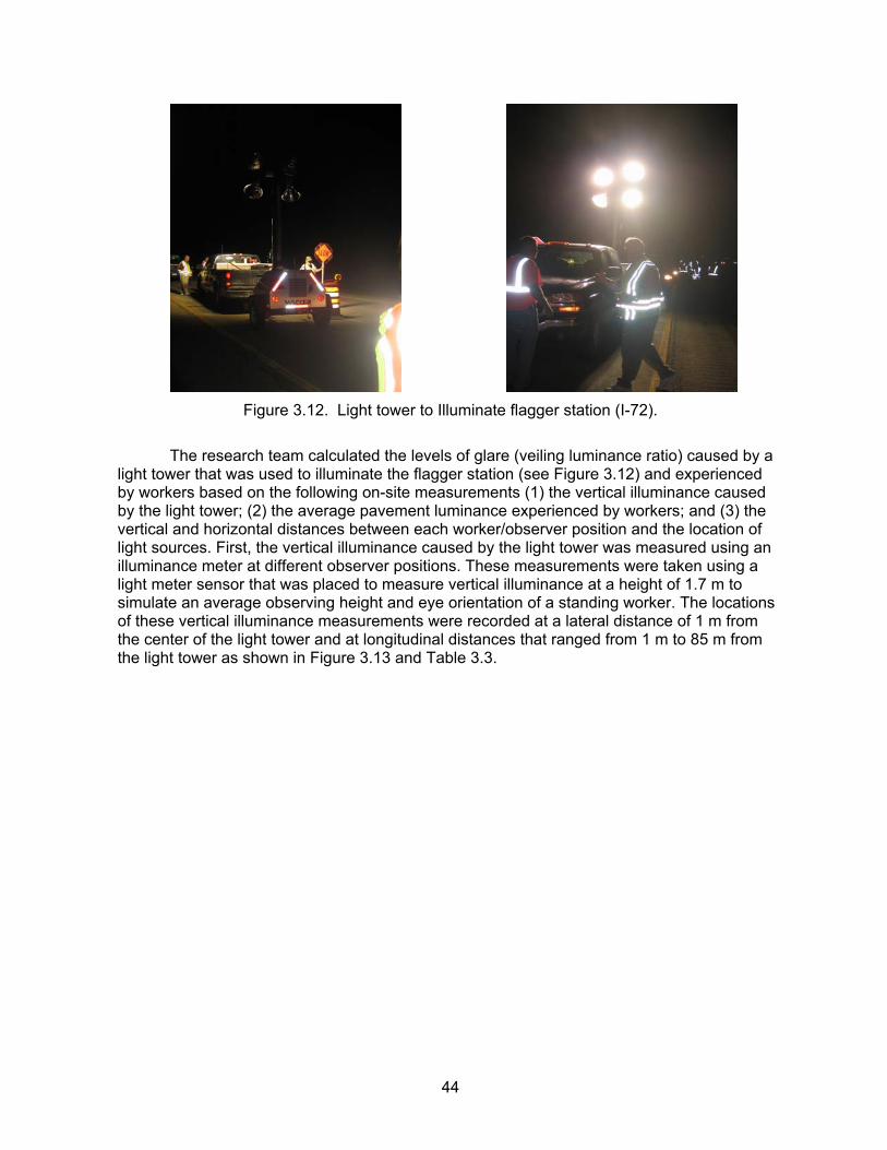
44
Figure 3.12. Light tower to Illuminate flagger station (I-72).
The research team calculated the levels of glare (veiling luminance ratio) caused by a light tower that was used to illuminate the flagger station (see Figure 3.12) and experienced by workers based on the following on-site measurements (1) the vertical illuminance caused by the light tower; (2) the average pavement luminance experienced by workers; and (3) the vertical and horizontal distances between each worker/observer position and the location of light sources. First, the vertical illuminance caused by the light tower was measured using an illuminance meter at different observer positions. These measurements were taken using a light meter sensor that was placed to measure vertical illuminance at a height of 1.7 m to simulate an average observing height and eye orientation of a standing worker. The locations of these vertical illuminance measurements were recorded at a lateral distance of 1 m from the center of the light tower and at longitudinal distances that ranged from 1 m to 85 m from the light tower as shown in Figure 3.13 and Table 3.3.
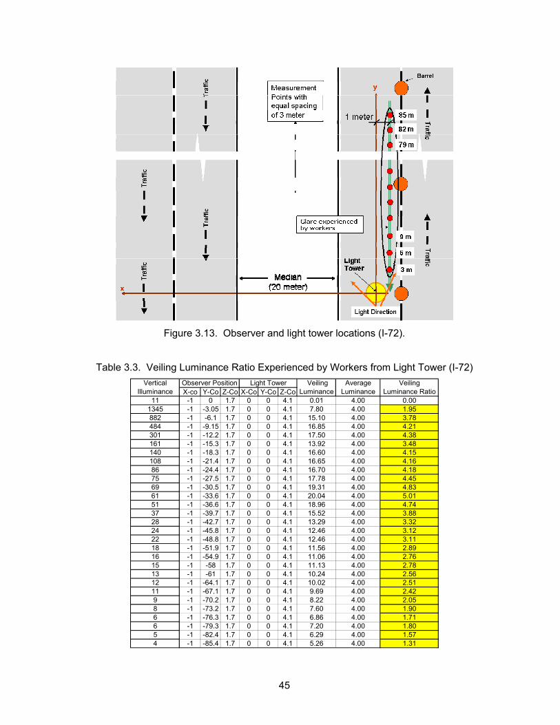
45
Figure 3.13. Observer and light tower locations (I-72).
Table 3.3. Veiling Luminance Ratio Experienced by Workers from Light Tower (I-72)
X-co Y-Co Z-Co X-Co Y-Co Z-Co11 -1 0 1.7 0 0 4.1 0.01 4.00 0.00
1345 -1 -3.05 1.7 0 0 4.1 7.80 4.00 1.95882 -1 -6.1 1.7 0 0 4.1 15.10 4.00 3.78484 -1 -9.15 1.7 0 0 4.1 16.85 4.00 4.21301 -1 -12.2 1.7 0 0 4.1 17.50 4.00 4.38161 -1 -15.3 1.7 0 0 4.1 13.92 4.00 3.48140 -1 -18.3 1.7 0 0 4.1 16.60 4.00 4.15108 -1 -21.4 1.7 0 0 4.1 16.65 4.00 4.1686 -1 -24.4 1.7 0 0 4.1 16.70 4.00 4.1875 -1 -27.5 1.7 0 0 4.1 17.78 4.00 4.4569 -1 -30.5 1.7 0 0 4.1 19.31 4.00 4.8361 -1 -33.6 1.7 0 0 4.1 20.04 4.00 5.0151 -1 -36.6 1.7 0 0 4.1 18.96 4.00 4.7437 -1 -39.7 1.7 0 0 4.1 15.52 4.00 3.8828 -1 -42.7 1.7 0 0 4.1 13.29 4.00 3.3224 -1 -45.8 1.7 0 0 4.1 12.46 4.00 3.1222 -1 -48.8 1.7 0 0 4.1 12.46 4.00 3.1118 -1 -51.9 1.7 0 0 4.1 11.56 4.00 2.8916 -1 -54.9 1.7 0 0 4.1 11.06 4.00 2.7615 -1 -58 1.7 0 0 4.1 11.13 4.00 2.7813 -1 -61 1.7 0 0 4.1 10.24 4.00 2.5612 -1 -64.1 1.7 0 0 4.1 10.02 4.00 2.5111 -1 -67.1 1.7 0 0 4.1 9.69 4.00 2.429 -1 -70.2 1.7 0 0 4.1 8.22 4.00 2.058 -1 -73.2 1.7 0 0 4.1 7.60 4.00 1.906 -1 -76.3 1.7 0 0 4.1 6.86 4.00 1.716 -1 -79.3 1.7 0 0 4.1 7.20 4.00 1.805 -1 -82.4 1.7 0 0 4.1 6.29 4.00 1.574 -1 -85.4 1.7 0 0 4.1 5.26 4.00 1.31
Vertical Illuminance
Observer Position Veiling Luminance Ratio
Veiling Luminance
Average Luminance
Light Tower
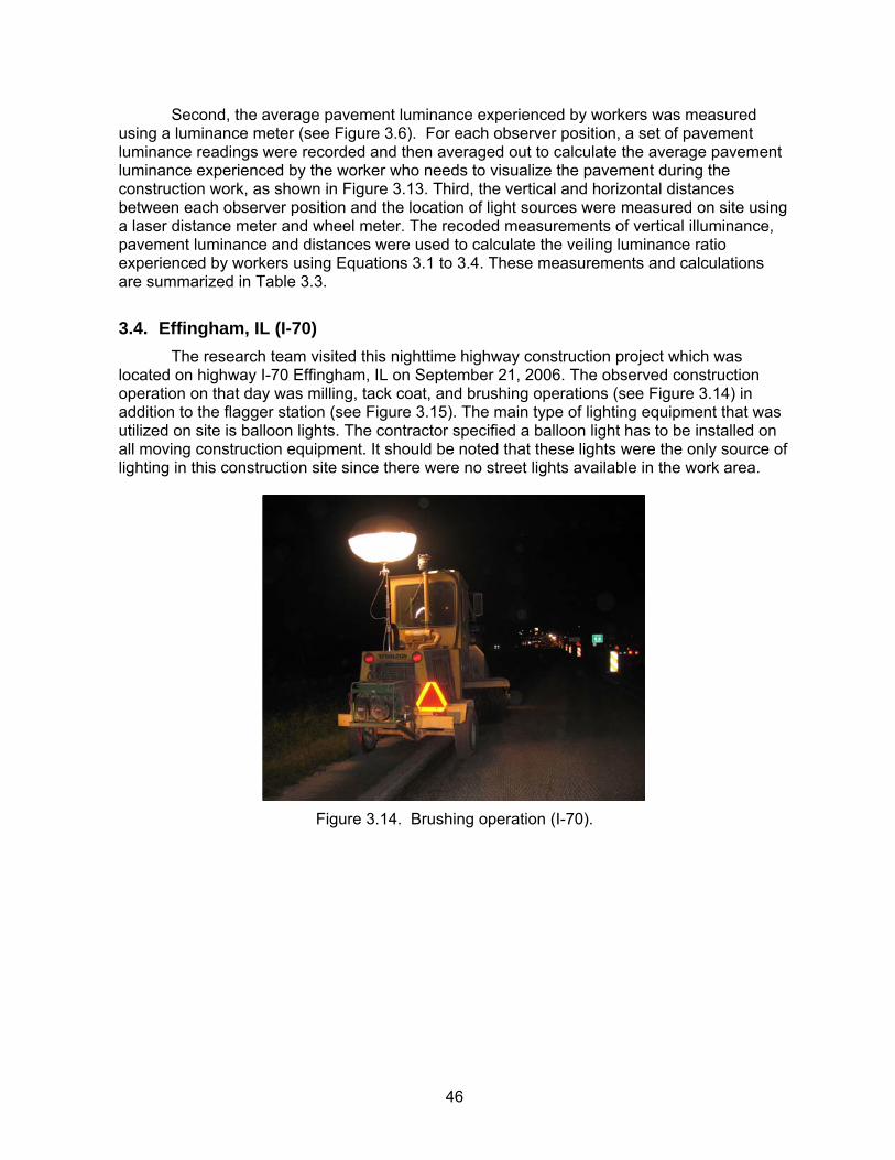
46
Second, the average pavement luminance experienced by workers was measured using a luminance meter (see Figure 3.6). For each observer position, a set of pavement luminance readings were recorded and then averaged out to calculate the average pavement luminance experienced by the worker who needs to visualize the pavement during the construction work, as shown in Figure 3.13. Third, the vertical and horizontal distances between each observer position and the location of light sources were measured on site using a laser distance meter and wheel meter. The recoded measurements of vertical illuminance, pavement luminance and distances were used to calculate the veiling luminance ratio experienced by workers using Equations 3.1 to 3.4. These measurements and calculations are summarized in Table 3.3.
3.4. Effingham, IL (I-70) The research team visited this nighttime highway construction project which was located on highway I-70 Effingham, IL on September 21, 2006. The observed construction operation on that day was milling, tack coat, and brushing operations (see Figure 3.14) in addition to the flagger station (see Figure 3.15). The main type of lighting equipment that was utilized on site is balloon lights. The contractor specified a balloon light has to be installed on all moving construction equipment. It should be noted that these lights were the only source of lighting in this construction site since there were no street lights available in the work area.
Figure 3.14. Brushing operation (I-70).
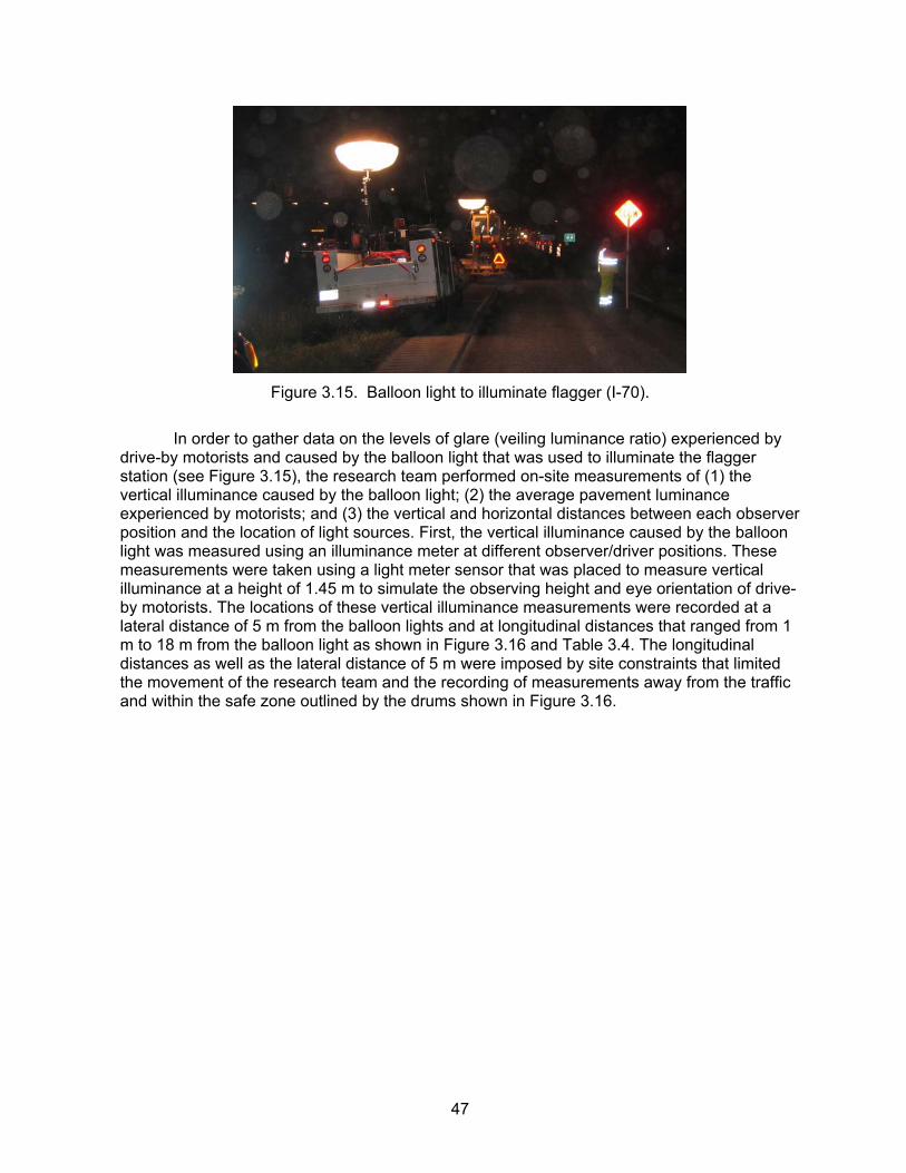
47
Figure 3.15. Balloon light to illuminate flagger (I-70).
In order to gather data on the levels of glare (veiling luminance ratio) experienced by drive-by motorists and caused by the balloon light that was used to illuminate the flagger station (see Figure 3.15), the research team performed on-site measurements of (1) the vertical illuminance caused by the balloon light; (2) the average pavement luminance experienced by motorists; and (3) the vertical and horizontal distances between each observer position and the location of light sources. First, the vertical illuminance caused by the balloon light was measured using an illuminance meter at different observer/driver positions. These measurements were taken using a light meter sensor that was placed to measure vertical illuminance at a height of 1.45 m to simulate the observing height and eye orientation of drive-by motorists. The locations of these vertical illuminance measurements were recorded at a lateral distance of 5 m from the balloon lights and at longitudinal distances that ranged from 1 m to 18 m from the balloon light as shown in Figure 3.16 and Table 3.4. The longitudinal distances as well as the lateral distance of 5 m were imposed by site constraints that limited the movement of the research team and the recording of measurements away from the traffic and within the safe zone outlined by the drums shown in Figure 3.16.

48
Figure 3.16. Observer and balloon light locations (I-70).
Table 3.4. Glare Measurements from Balloon Lights (I-70)
X-co Y-Co Z-Co X-Co Y-Co Z-Co10.0 5 0 1.45 0 0 3.1 0.01 0.50 0.0222.0 5 -1.53 1.45 0 0 3.1 0.04 0.50 0.0829.0 5 -3.05 1.45 0 0 3.1 0.09 0.50 0.1729.0 5 -4.58 1.45 0 0 3.1 0.13 0.50 0.2624.0 5 -6.1 1.45 0 0 3.1 0.16 0.50 0.3220.0 5 -7.63 1.45 0 0 3.1 0.18 0.50 0.3715.0 5 -9.15 1.45 0 0 3.1 0.19 0.50 0.3713.0 5 -10.7 1.45 0 0 3.1 0.21 0.50 0.4211.0 5 -12.2 1.45 0 0 3.1 0.23 0.50 0.4510.0 5 -13.7 1.45 0 0 3.1 0.25 0.50 0.518.0 5 -15.3 1.45 0 0 3.1 0.25 0.50 0.497.0 5 -16.8 1.45 0 0 3.1 0.26 0.50 0.515.0 5 -18.3 1.45 0 0 3.1 0.21 0.50 0.43
Balloon Light Veiling Luminance Ratio
Veiling Luminance
Average Pavement Luminance
Vertical Illuminance
Observer Position
Second, the average pavement luminance experienced by motorists was measured using a luminance meter (see Figure 3.6). For each driver/observer position, a set of pavement luminance readings were recorded and then averaged out to calculate the average pavement luminance experienced by the driver at the considered observation point, as shown
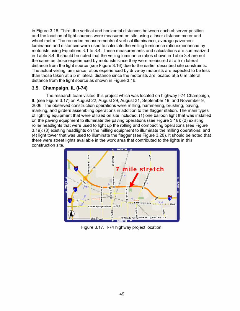
49
in Figure 3.16. Third, the vertical and horizontal distances between each observer position and the location of light sources were measured on site using a laser distance meter and wheel meter. The recorded measurements of vertical illuminance, average pavement luminance and distances were used to calculate the veiling luminance ratio experienced by motorists using Equations 3.1 to 3.4. These measurements and calculations are summarized in Table 3.4. It should be noted that the veiling luminance ratios shown in Table 3.4 are not the same as those experienced by motorists since they were measured at a 5 m lateral distance from the light source (see Figure 3.16) due to the earlier described site constraints. The actual veiling luminance ratios experienced by drive-by motorists are expected to be less than those taken at a 5 m lateral distance since the motorists are located at a 6 m lateral distance from the light source as shown in Figure 3.16.
3.5. Champaign, IL (I-74) The research team visited this project which was located on highway I-74 Champaign, IL (see Figure 3.17) on August 22, August 29, August 31, September 19, and November 9, 2006. The observed construction operations were milling, hammering, brushing, paving, marking, and girders assembling operations in addition to the flagger station. The main types of lighting equipment that were utilized on site included: (1) one balloon light that was installed on the paving equipment to illuminate the paving operations (see Figure 3.18); (2) existing roller headlights that were used to light up the rolling and compacting operations (see Figure 3.19); (3) existing headlights on the milling equipment to illuminate the milling operations; and (4) light tower that was used to illuminate the flagger (see Figure 3.20). It should be noted that there were street lights available in the work area that contributed to the lights in this construction site.
Figure 3.17. I-74 highway project location.
7 mile stretch
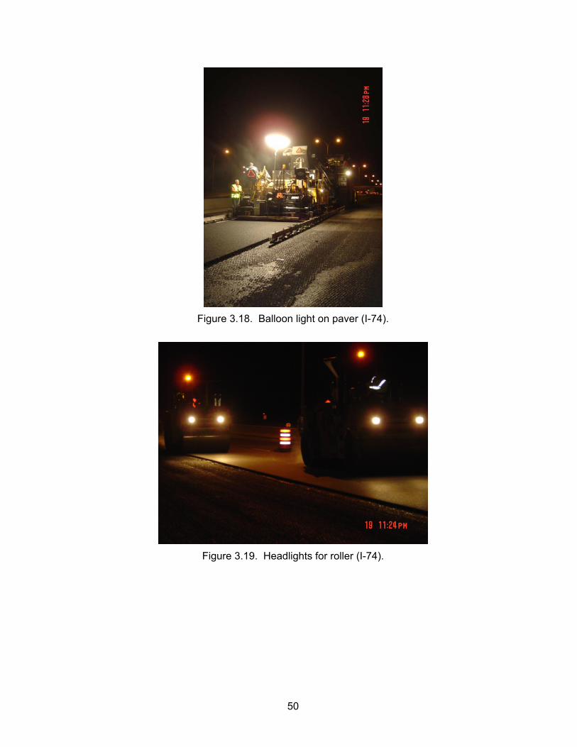
50
Figure 3.18. Balloon light on paver (I-74).
Figure 3.19. Headlights for roller (I-74).
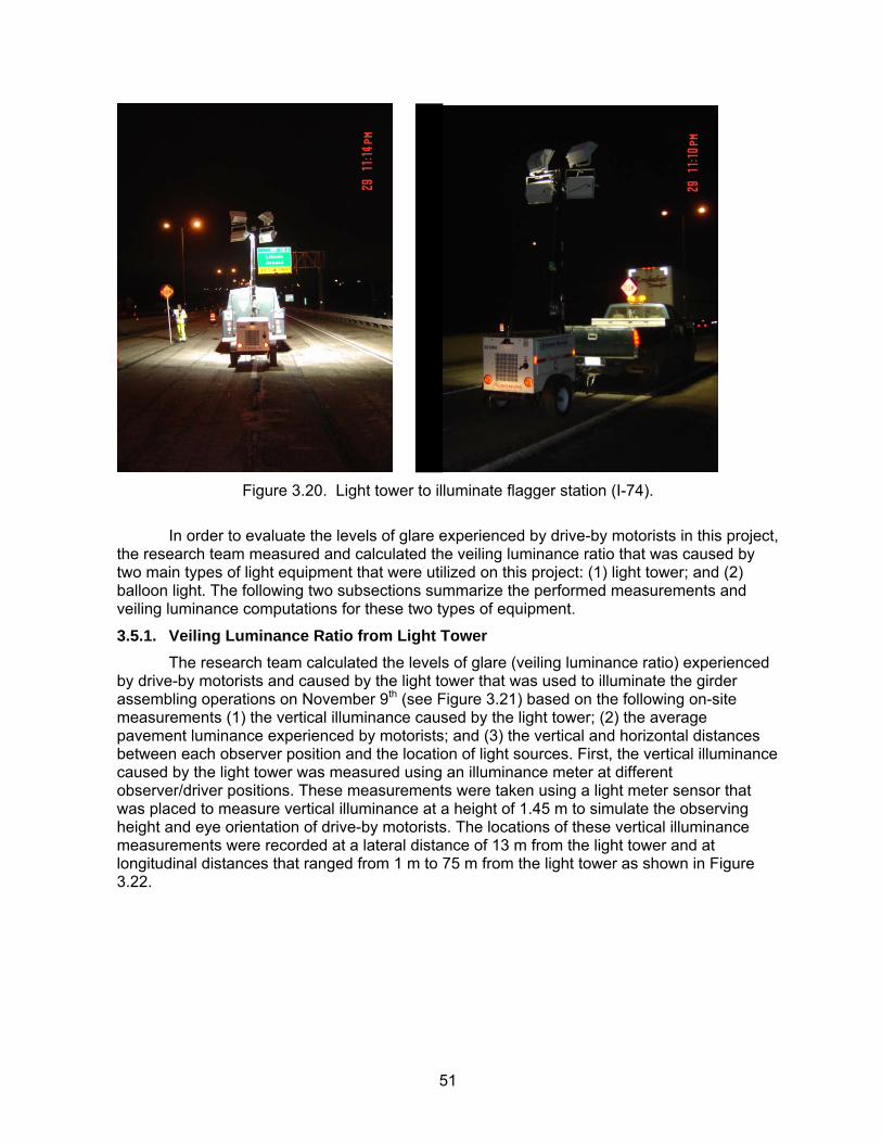
51
Figure 3.20. Light tower to illuminate flagger station (I-74).
In order to evaluate the levels of glare experienced by drive-by motorists in this project, the research team measured and calculated the veiling luminance ratio that was caused by two main types of light equipment that were utilized on this project: (1) light tower; and (2) balloon light. The following two subsections summarize the performed measurements and veiling luminance computations for these two types of equipment.
3.5.1. Veiling Luminance Ratio from Light Tower The research team calculated the levels of glare (veiling luminance ratio) experienced by drive-by motorists and caused by the light tower that was used to illuminate the girder assembling operations on November 9th (see Figure 3.21) based on the following on-site measurements (1) the vertical illuminance caused by the light tower; (2) the average pavement luminance experienced by motorists; and (3) the vertical and horizontal distances between each observer position and the location of light sources. First, the vertical illuminance caused by the light tower was measured using an illuminance meter at different observer/driver positions. These measurements were taken using a light meter sensor that was placed to measure vertical illuminance at a height of 1.45 m to simulate the observing height and eye orientation of drive-by motorists. The locations of these vertical illuminance measurements were recorded at a lateral distance of 13 m from the light tower and at longitudinal distances that ranged from 1 m to 75 m from the light tower as shown in Figure 3.22.
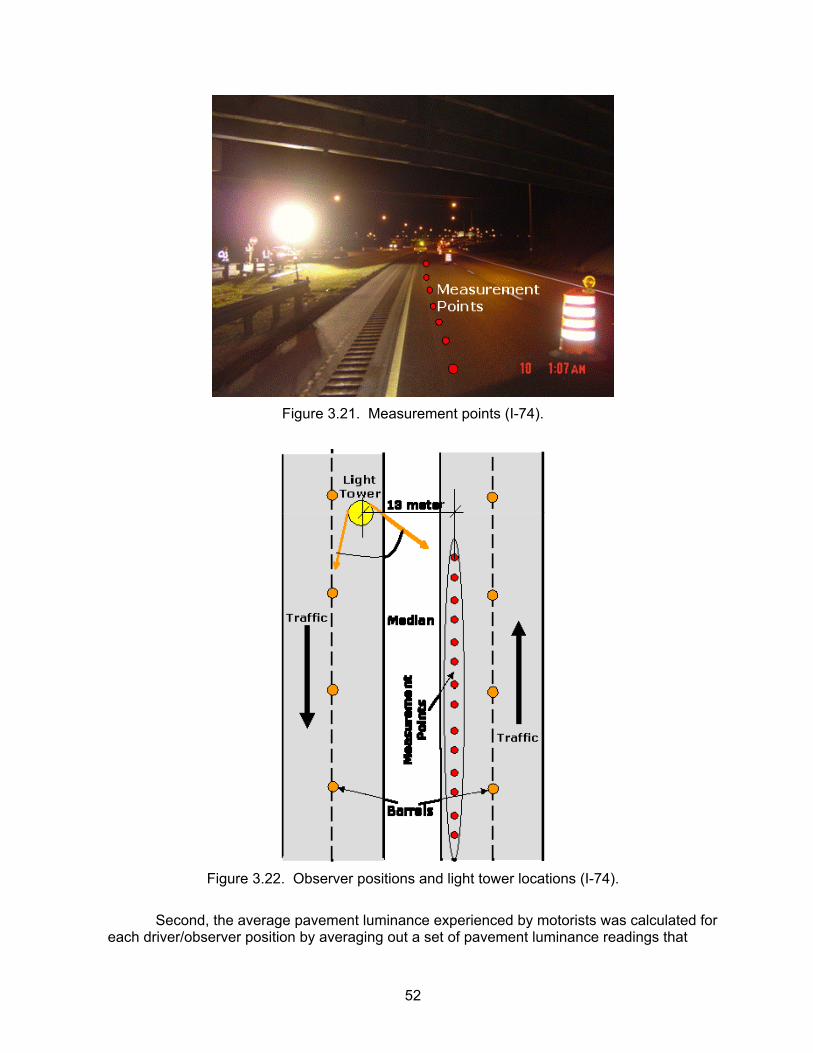
52
Figure 3.21. Measurement points (I-74).
Figure 3.22. Observer positions and light tower locations (I-74).
Second, the average pavement luminance experienced by motorists was calculated for each driver/observer position by averaging out a set of pavement luminance readings that
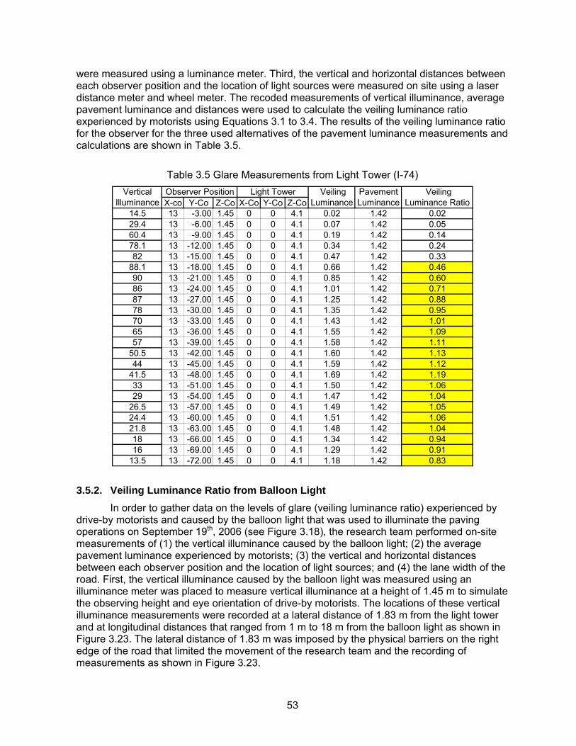
53
were measured using a luminance meter. Third, the vertical and horizontal distances between each observer position and the location of light sources were measured on site using a laser distance meter and wheel meter. The recoded measurements of vertical illuminance, average pavement luminance and distances were used to calculate the veiling luminance ratio experienced by motorists using Equations 3.1 to 3.4. The results of the veiling luminance ratio for the observer for the three used alternatives of the pavement luminance measurements and calculations are shown in Table 3.5.
Table 3.5 Glare Measurements from Light Tower (I-74)
X-co Y-Co Z-Co X-Co Y-Co Z-Co14.5 13 -3.00 1.45 0 0 4.1 0.02 1.42 0.0229.4 13 -6.00 1.45 0 0 4.1 0.07 1.42 0.0560.4 13 -9.00 1.45 0 0 4.1 0.19 1.42 0.1478.1 13 -12.00 1.45 0 0 4.1 0.34 1.42 0.2482 13 -15.00 1.45 0 0 4.1 0.47 1.42 0.33
88.1 13 -18.00 1.45 0 0 4.1 0.66 1.42 0.4690 13 -21.00 1.45 0 0 4.1 0.85 1.42 0.6086 13 -24.00 1.45 0 0 4.1 1.01 1.42 0.7187 13 -27.00 1.45 0 0 4.1 1.25 1.42 0.8878 13 -30.00 1.45 0 0 4.1 1.35 1.42 0.9570 13 -33.00 1.45 0 0 4.1 1.43 1.42 1.0165 13 -36.00 1.45 0 0 4.1 1.55 1.42 1.0957 13 -39.00 1.45 0 0 4.1 1.58 1.42 1.11
50.5 13 -42.00 1.45 0 0 4.1 1.60 1.42 1.1344 13 -45.00 1.45 0 0 4.1 1.59 1.42 1.12
41.5 13 -48.00 1.45 0 0 4.1 1.69 1.42 1.1933 13 -51.00 1.45 0 0 4.1 1.50 1.42 1.0629 13 -54.00 1.45 0 0 4.1 1.47 1.42 1.04
26.5 13 -57.00 1.45 0 0 4.1 1.49 1.42 1.0524.4 13 -60.00 1.45 0 0 4.1 1.51 1.42 1.0621.8 13 -63.00 1.45 0 0 4.1 1.48 1.42 1.0418 13 -66.00 1.45 0 0 4.1 1.34 1.42 0.9416 13 -69.00 1.45 0 0 4.1 1.29 1.42 0.91
13.5 13 -72.00 1.45 0 0 4.1 1.18 1.42 0.83
Veiling Luminance
Pavement Luminance
Veiling Luminance Ratio
Light TowerVertical Illuminance
Observer Position
3.5.2. Veiling Luminance Ratio from Balloon Light In order to gather data on the levels of glare (veiling luminance ratio) experienced by drive-by motorists and caused by the balloon light that was used to illuminate the paving operations on September 19th, 2006 (see Figure 3.18), the research team performed on-site measurements of (1) the vertical illuminance caused by the balloon light; (2) the average pavement luminance experienced by motorists; (3) the vertical and horizontal distances between each observer position and the location of light sources; and (4) the lane width of the road. First, the vertical illuminance caused by the balloon light was measured using an illuminance meter was placed to measure vertical illuminance at a height of 1.45 m to simulate the observing height and eye orientation of drive-by motorists. The locations of these vertical illuminance measurements were recorded at a lateral distance of 1.83 m from the light tower and at longitudinal distances that ranged from 1 m to 18 m from the balloon light as shown in Figure 3.23. The lateral distance of 1.83 m was imposed by the physical barriers on the right edge of the road that limited the movement of the research team and the recording of measurements as shown in Figure 3.23.

54
Figure 3.23. Observer and balloon light locations (I-74).
Second, the average pavement luminance experienced by motorists was measured using a luminance meter (see Figure 3.6). For each driver/observer position, a set of pavement luminance readings were recorded and then averaged out to calculate the average pavement luminance experienced by the driver at the considered observation point, as shown in Figure 3.23. Third, the vertical and horizontal distances between each observer position and the location of light sources were measured on site using a laser distance meter and wheel meter as shown in Figure 3.7. Fourth, the lane width was measured using a laser distance meter and wheel meter as shown in Figure 3.7. The above recorded measurements of vertical illuminance, average pavement luminance and distances were used to calculate the veiling luminance ratio experienced by motorists using Equations 3.1 to 3.4. These measurements and calculations are summarized in Table 3.6. It should be noted that the veiling luminance ratios shown in Table 3.6 are not the same as those experienced by motorists since they were measured at a 1.83 m lateral distance from the light source (see Figure 3.23) due to the earlier described site constraints. The actual veiling luminance ratios experienced by drive-by motorists are expected to be less than those taken at a 1.83 m lateral distance since the motorists are located at a 3.75 m lateral distance from the light source as shown in Figure 3.23.

55
Table 3.6. Glare Measurements from Balloon Lights (I-74)
X-co Y-Co Z-Co X-Co Y-Co Z-Co17.0 -1.83 0 1.45 0 0 4.5 0.02 1.00 0.0227.0 -1.83 -0.92 1.45 0 0 4.5 0.05 1.00 0.0573.0 -1.83 -1.83 1.45 0 0 4.5 0.18 1.00 0.1893.0 -1.83 -2.75 1.45 0 0 4.5 0.33 1.00 0.33
102.0 -1.83 -3.66 1.45 0 0 4.5 0.50 1.00 0.50104.0 -1.83 -4.58 1.45 0 0 4.5 0.69 1.00 0.6999.0 -1.83 -5.49 1.45 0 0 4.5 0.87 1.00 0.8788.0 -1.83 -6.41 1.45 0 0 4.5 0.98 1.00 0.9875.0 -1.83 -7.32 1.45 0 0 4.5 1.05 1.00 1.0566.0 -1.83 -8.24 1.45 0 0 4.5 1.12 1.00 1.1256.0 -1.83 -9.15 1.45 0 0 4.5 1.15 1.00 1.1551.0 -1.83 -10.1 1.45 0 0 4.5 1.23 1.00 1.2343.0 -1.83 -11 1.45 0 0 4.5 1.21 1.00 1.2137.0 -1.83 -11.9 1.45 0 0 4.5 1.21 1.00 1.2132.0 -1.83 -12.8 1.45 0 0 4.5 1.19 1.00 1.1928.0 -1.83 -13.7 1.45 0 0 4.5 1.18 1.00 1.1822.0 -1.83 -14.6 1.45 0 0 4.5 1.04 1.00 1.0422.0 -1.83 -15.6 1.45 0 0 4.5 1.16 1.00 1.1619.0 -1.83 -16.5 1.45 0 0 4.5 1.11 1.00 1.1118.0 -1.83 -17.4 1.45 0 0 4.5 1.16 1.00 1.1617.0 -1.83 -18.3 1.45 0 0 4.5 1.21 1.00 1.21
Vertical Illuminance
Observer Position Veiling Luminance Ratio
Veiling Luminance
Average Pavement Luminance
Balloon Light
3.6. Main Findings The research team observed several construction operations during the aforementioned site visits. The observed construction operations included milling, paving, compacting, patching, hammering, and girder assembling in addition to the flagger station. The types of lighting equipment that were utilized on these sites included light towers, balloon lights, marine lights, and existing headlights of construction equipment such as roller and milling equipment. Table 3.7 summarizes the observed construction operations and the typical lighting equipment used in each observed operation.
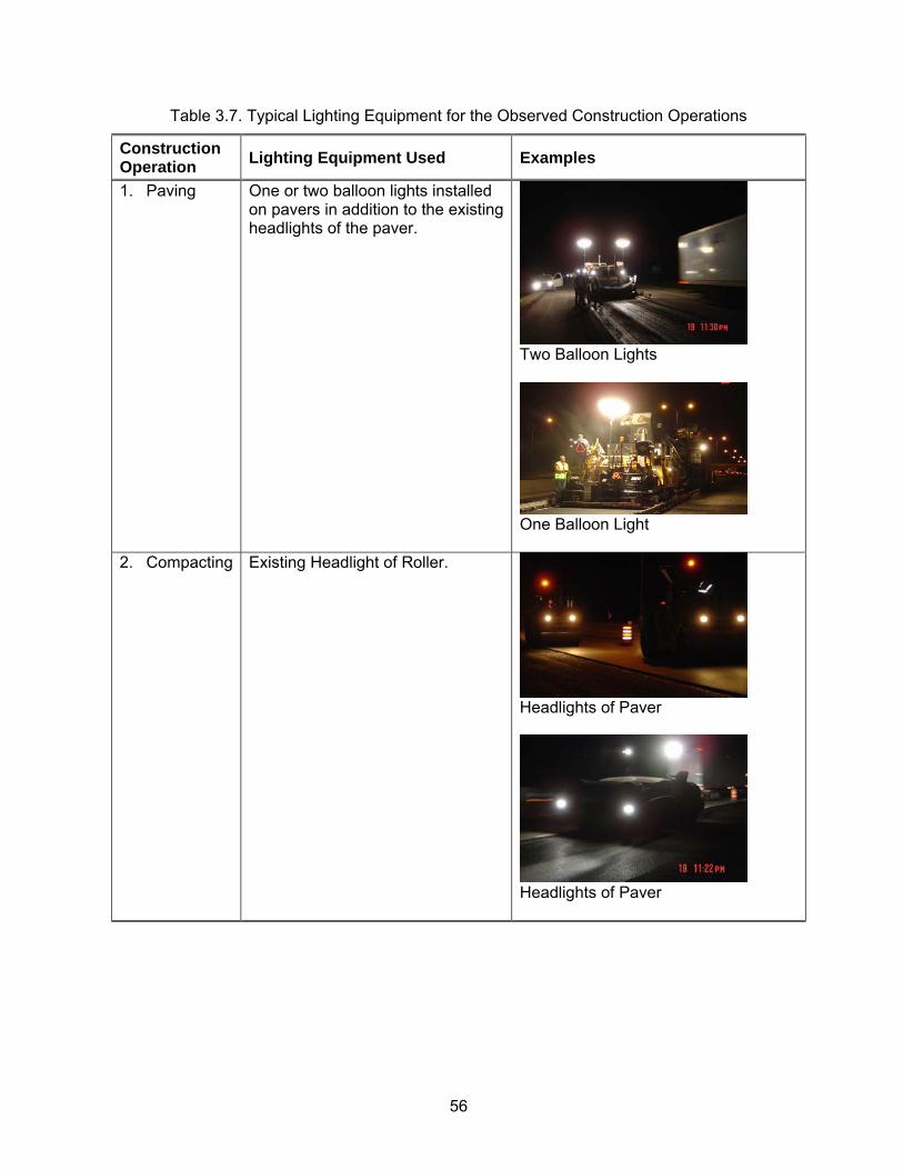
56
Table 3.7. Typical Lighting Equipment for the Observed Construction Operations
Construction Operation Lighting Equipment Used Examples
1. Paving One or two balloon lights installed on pavers in addition to the existing headlights of the paver.
Two Balloon Lights
One Balloon Light
2. Compacting Existing Headlight of Roller.
Headlights of Paver
Headlights of Paver
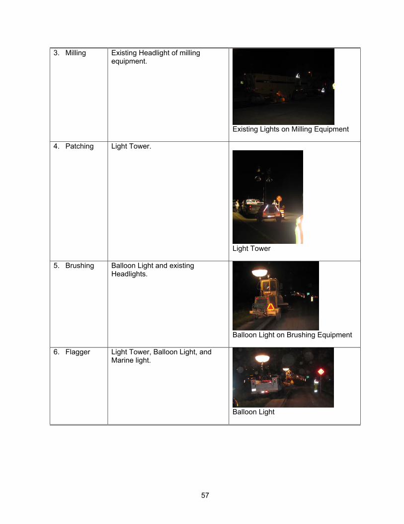
57
3. Milling Existing Headlight of milling equipment.
Existing Lights on Milling Equipment
4. Patching Light Tower.
Light Tower
5. Brushing Balloon Light and existing Headlights.
Balloon Light on Brushing Equipment
6. Flagger Light Tower, Balloon Light, and Marine light.
Balloon Light
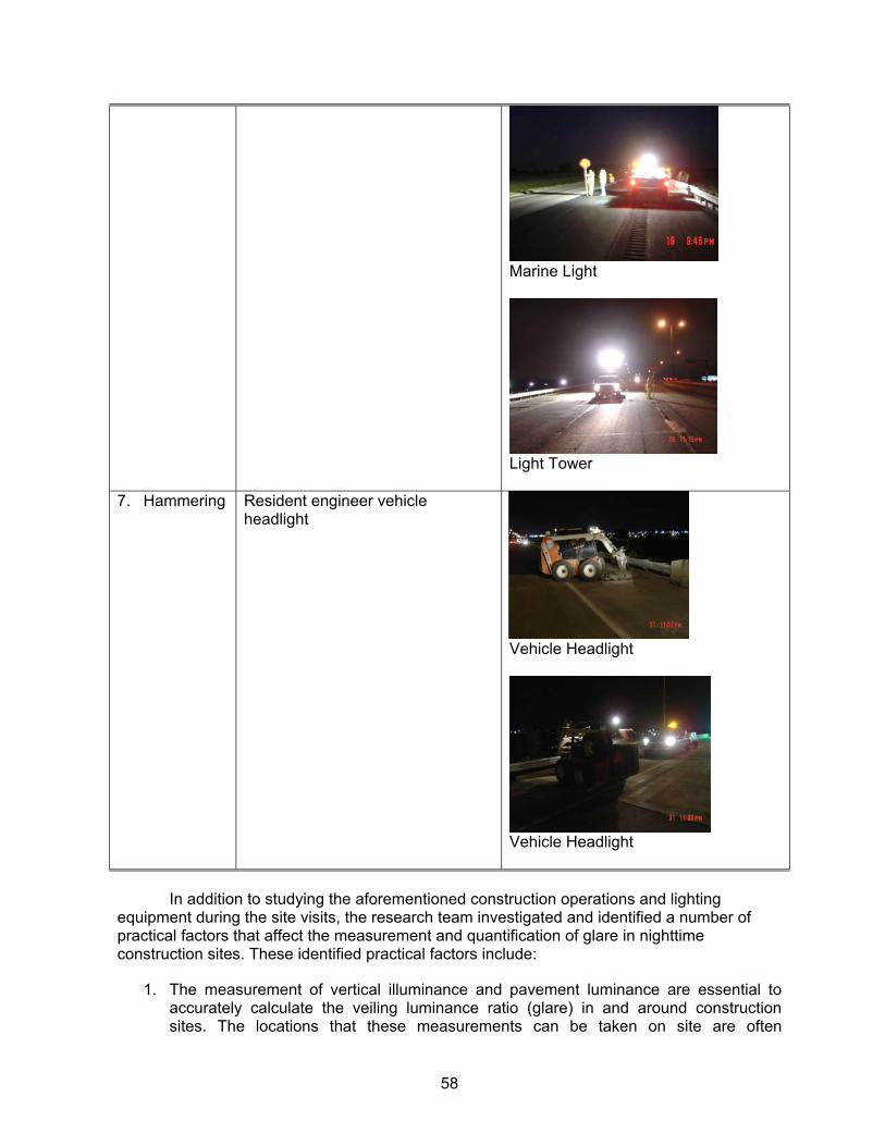
58
Marine Light
Light Tower
7. Hammering Resident engineer vehicle headlight
Vehicle Headlight
Vehicle Headlight
In addition to studying the aforementioned construction operations and lighting equipment during the site visits, the research team investigated and identified a number of practical factors that affect the measurement and quantification of glare in nighttime construction sites. These identified practical factors include:
1. The measurement of vertical illuminance and pavement luminance are essential to accurately calculate the veiling luminance ratio (glare) in and around construction sites. The locations that these measurements can be taken on site are often
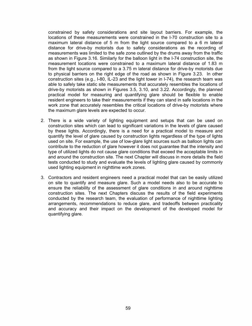
59
constrained by safety considerations and site layout barriers. For example, the locations of these measurements were constrained in the I-70 construction site to a maximum lateral distance of 5 m from the light source compared to a 6 m lateral distance for drive-by motorists due to safety considerations as the recording of measurements was limited to the safe zone outlined by the drums away from the traffic as shown in Figure 3.16. Similarly for the balloon light in the I-74 construction site, the measurement locations were constrained to a maximum lateral distance of 1.83 m from the light source compared to a 3.75 m lateral distance for drive-by motorists due to physical barriers on the right edge of the road as shown in Figure 3.23. In other construction sites (e.g., I-80, IL-23 and the light tower in I-74), the research team was able to safely take static site measurements that accurately resembles the locations of drive-by motorists as shown in Figures 3.5, 3.10, and 3.22. Accordingly, the planned practical model for measuring and quantifying glare should be flexible to enable resident engineers to take their measurements if they can stand in safe locations in the work zone that accurately resembles the critical locations of drive-by motorists where the maximum glare levels are expected to occur.
2. There is a wide variety of lighting equipment and setups that can be used on construction sites which can lead to significant variations in the levels of glare caused by these lights. Accordingly, there is a need for a practical model to measure and quantify the level of glare caused by construction lights regardless of the type of lights used on site. For example, the use of low-glare light sources such as balloon lights can contribute to the reduction of glare however it does not guarantee that the intensity and type of utilized lights do not cause glare conditions that exceed the acceptable limits in and around the construction site. The next Chapter will discuss in more details the field tests conducted to study and evaluate the levels of lighting glare caused by commonly used lighting equipment in nighttime work zones.
3. Contractors and resident engineers need a practical model that can be easily utilized on site to quantify and measure glare. Such a model needs also to be accurate to ensure the reliability of the assessment of glare conditions in and around nighttime construction sites. The next Chapters discuss the results of the field experiments conducted by the research team, the evaluation of performance of nighttime lighting arrangements, recommendations to reduce glare, and tradeoffs between practicality and accuracy and their impact on the development of the developed model for quantifying glare.
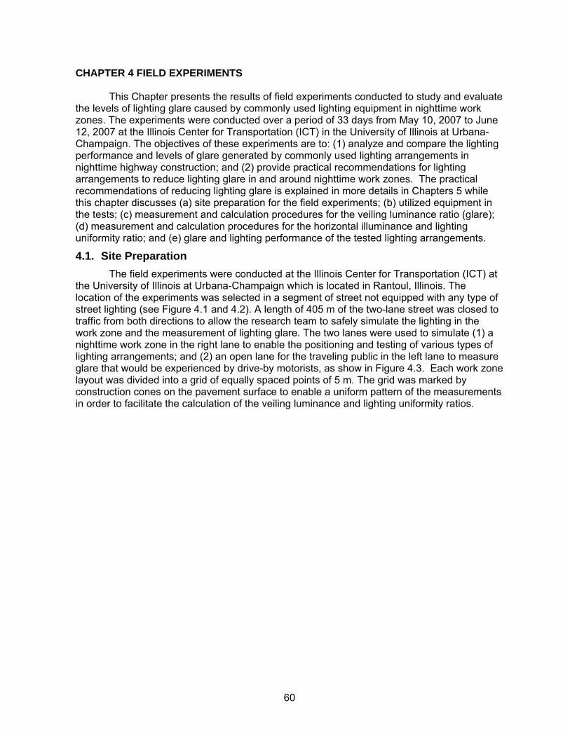
60
CHAPTER 4 FIELD EXPERIMENTS 4. This Chapter presents the results of field experiments conducted to study and evaluate the levels of lighting glare caused by commonly used lighting equipment in nighttime work zones. The experiments were conducted over a period of 33 days from May 10, 2007 to June 12, 2007 at the Illinois Center for Transportation (ICT) in the University of Illinois at Urbana-Champaign. The objectives of these experiments are to: (1) analyze and compare the lighting performance and levels of glare generated by commonly used lighting arrangements in nighttime highway construction; and (2) provide practical recommendations for lighting arrangements to reduce lighting glare in and around nighttime work zones. The practical recommendations of reducing lighting glare is explained in more details in Chapters 5 while this chapter discusses (a) site preparation for the field experiments; (b) utilized equipment in the tests; (c) measurement and calculation procedures for the veiling luminance ratio (glare); (d) measurement and calculation procedures for the horizontal illuminance and lighting uniformity ratio; and (e) glare and lighting performance of the tested lighting arrangements.
4.1. Site Preparation The field experiments were conducted at the Illinois Center for Transportation (ICT) at the University of Illinois at Urbana-Champaign which is located in Rantoul, Illinois. The location of the experiments was selected in a segment of street not equipped with any type of street lighting (see Figure 4.1 and 4.2). A length of 405 m of the two-lane street was closed to traffic from both directions to allow the research team to safely simulate the lighting in the work zone and the measurement of lighting glare. The two lanes were used to simulate (1) a nighttime work zone in the right lane to enable the positioning and testing of various types of lighting arrangements; and (2) an open lane for the traveling public in the left lane to measure glare that would be experienced by drive-by motorists, as show in Figure 4.3. Each work zone layout was divided into a grid of equally spaced points of 5 m. The grid was marked by construction cones on the pavement surface to enable a uniform pattern of the measurements in order to facilitate the calculation of the veiling luminance and lighting uniformity ratios.
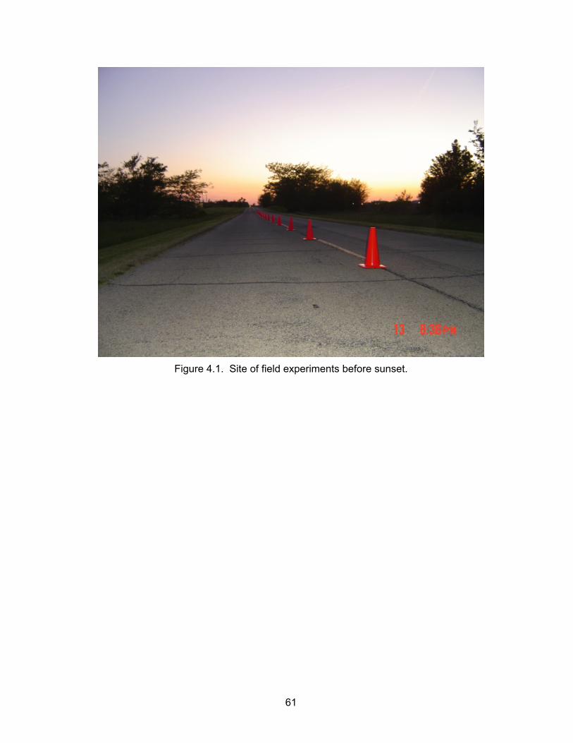
61
Figure 4.1. Site of field experiments before sunset.
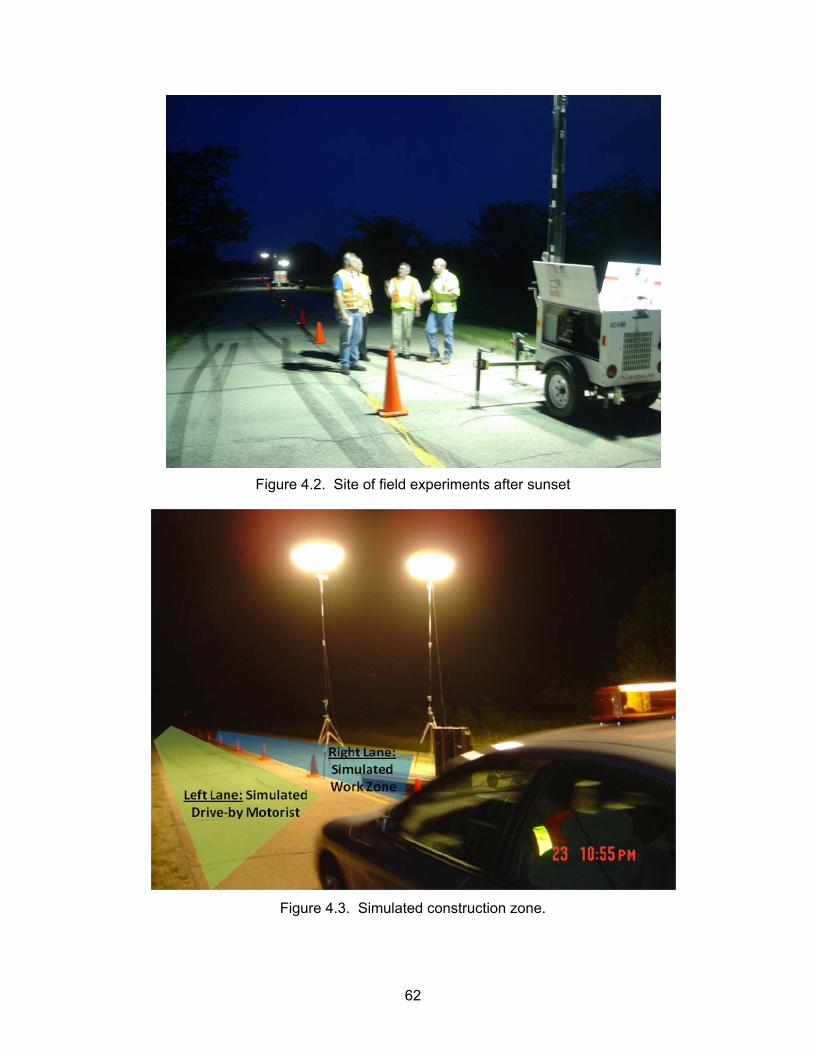
62
Figure 4.2. Site of field experiments after sunset
Figure 4.3. Simulated construction zone.

63
4.2. Utilized Equipment The field experiments evaluated the performance of three types of lighting equipment (balloon lights from Accenting Images Inc., Nite Lite from Protection Services Inc., and one rented adjustable light tower) and utilized four types of measurement equipment (illuminance meter, luminance meter, distance measurement meters, and angle locators). The following sections provide a brief description of each of these lighting and measurement equipment:
4.2.1. Balloon Lights
Three balloon lights were utilized in the field experiments. Each balloon light contains two 1000-watt halogen bulbs with a maximum light output of 54,000 Lumens and the capability to illuminate up to 500m2. The balloon light weighs 8 kg and is 1.1 m in diameter and it inflates with an internal fan. Each balloon light comes with a 5.8 m stand that was used to simulate and test the typical heights that were encountered during the site visits to a number of highway construction zones, as shown in Figure 4.4.
Figure 4.4. Balloon lights.
4.2.2. Nite Lite The Nite Lite is a portable construction light with a 400 watt Metal Halide lamp in a dome shape that is coated with a light diffusing compound, as shown in Figure 4.5. The light weighs 11.8 kg with a diameter of 0.635 m and it stores securely in its custom foam padded carry/storage case. Moreover, Nite Lite draws 4 amps at 120 volts AC, and comes standard with a 7.3 m grounded plug. Light output is rated at 42,000 Lumens which can illuminate an area of 1,395 m2.

64
Figure 4.5. Nite lite.
4.2.3. Light Tower One light tower was utilized in this experiment. The light tower is equipped with four 1000-watt metal halide luminaries, as shown in Figure 4.6. Aiming and rotation angles of all luminaries are adjustable in all directions, and mounting height of luminaries can be extended up to 8.5 m.
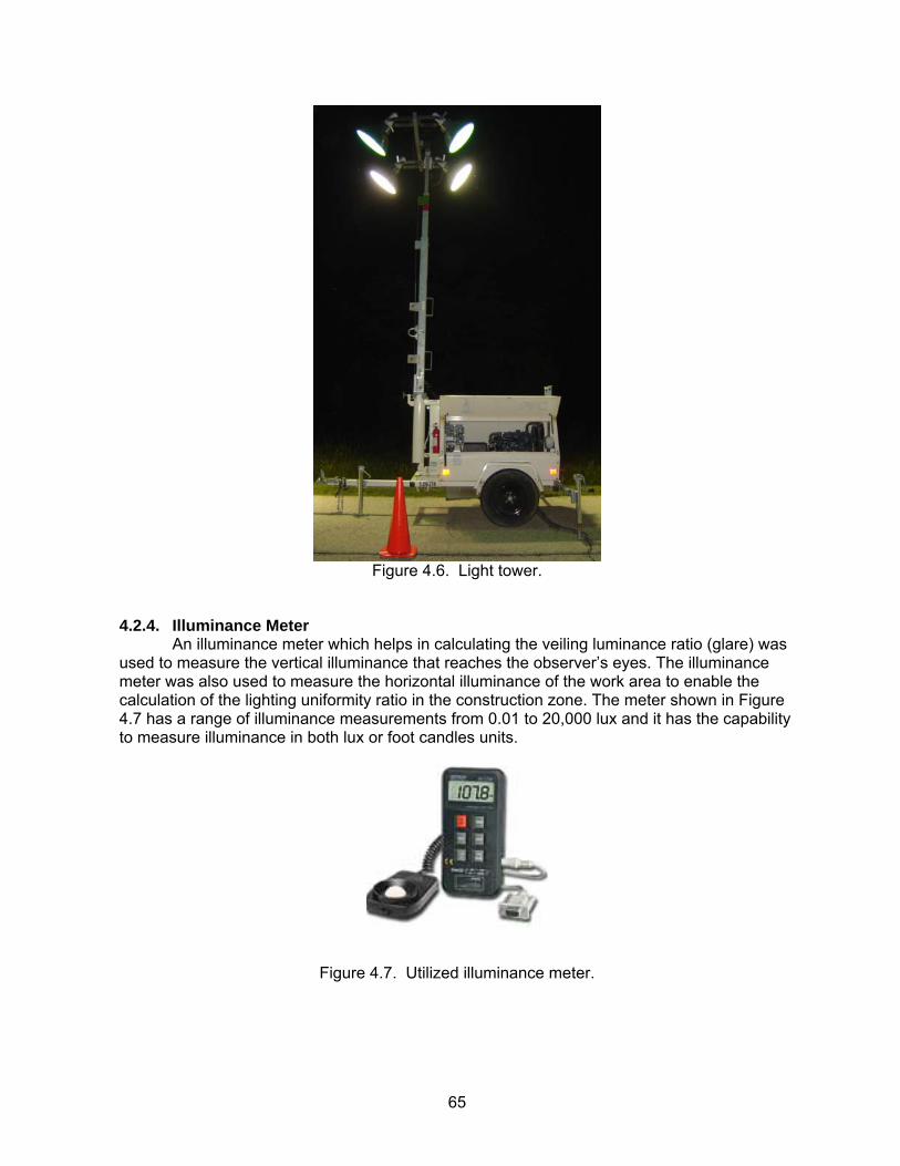
65
Figure 4.6. Light tower.
4.2.4. Illuminance Meter An illuminance meter which helps in calculating the veiling luminance ratio (glare) was used to measure the vertical illuminance that reaches the observer’s eyes. The illuminance meter was also used to measure the horizontal illuminance of the work area to enable the calculation of the lighting uniformity ratio in the construction zone. The meter shown in Figure 4.7 has a range of illuminance measurements from 0.01 to 20,000 lux and it has the capability to measure illuminance in both lux or foot candles units.
Figure 4.7. Utilized illuminance meter.
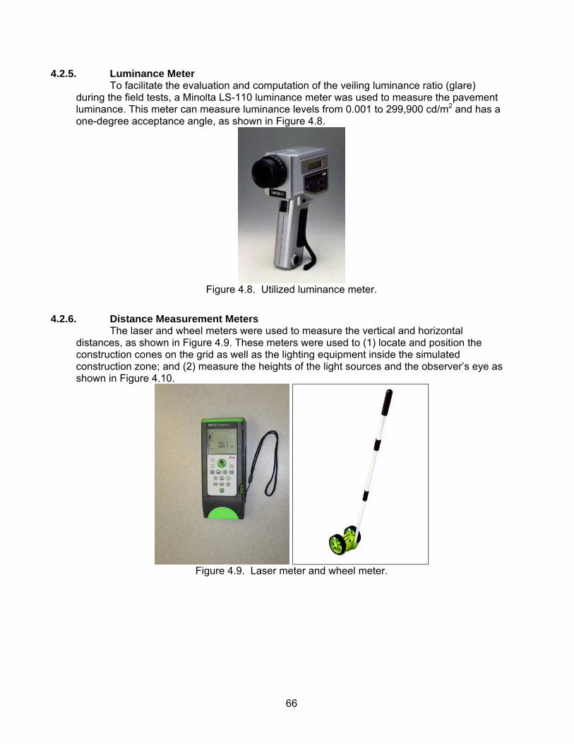
66
4.2.5. Luminance Meter To facilitate the evaluation and computation of the veiling luminance ratio (glare) during the field tests, a Minolta LS-110 luminance meter was used to measure the pavement luminance. This meter can measure luminance levels from 0.001 to 299,900 cd/m2 and has a one-degree acceptance angle, as shown in Figure 4.8.
Figure 4.8. Utilized luminance meter.
4.2.6. Distance Measurement Meters
The laser and wheel meters were used to measure the vertical and horizontal distances, as shown in Figure 4.9. These meters were used to (1) locate and position the construction cones on the grid as well as the lighting equipment inside the simulated construction zone; and (2) measure the heights of the light sources and the observer’s eye as shown in Figure 4.10.
Figure 4.9. Laser meter and wheel meter.
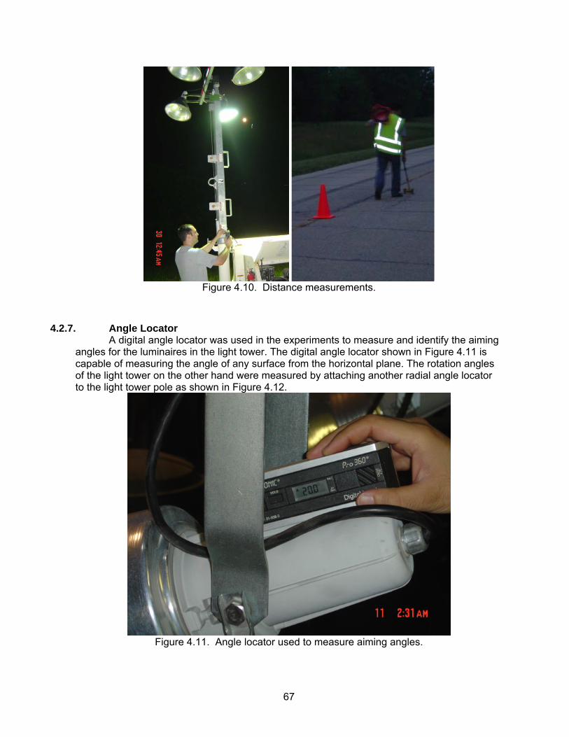
67
Figure 4.10. Distance measurements.
4.2.7. Angle Locator A digital angle locator was used in the experiments to measure and identify the aiming angles for the luminaires in the light tower. The digital angle locator shown in Figure 4.11 is capable of measuring the angle of any surface from the horizontal plane. The rotation angles of the light tower on the other hand were measured by attaching another radial angle locator to the light tower pole as shown in Figure 4.12.
Figure 4.11. Angle locator used to measure aiming angles.
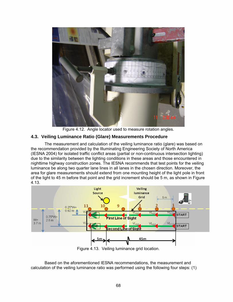
68
Figure 4.12. Angle locator used to measure rotation angles.
4.3. Veiling Luminance Ratio (Glare) Measurements Procedure The measurement and calculation of the veiling luminance ratio (glare) was based on the recommendation provided by the Illuminating Engineering Society of North America (IESNA 2004) for isolated traffic conflict areas (partial or non-continuous intersection lighting) due to the similarity between the lighting conditions in these areas and those encountered in nighttime highway construction zones. The IESNA recommends that test points for the veiling luminance be along two quarter lane lines in all lanes in the chosen direction. Moreover, the area for glare measurements should extend from one mounting height of the light pole in front of the light to 45 m before that point and the grid increment should be 5 m, as shown in Figure 4.13.
Figure 4.13. Veiling luminance grid location.
Based on the aforementioned IESNA recommendations, the measurement and calculation of the veiling luminance ratio was performed using the following four steps: (1)
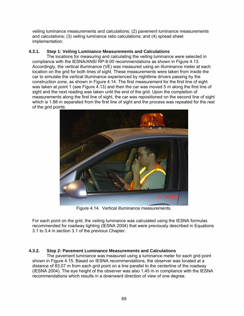
69
veiling luminance measurements and calculations; (2) pavement luminance measurements and calculations; (3) veiling luminance ratio calculations; and (4) spread sheet implementation.
4.3.1. Step 1: Veiling Luminance Measurements and Calculations
The locations for measuring and calculating the veiling luminance were selected in compliance with the IESNA/ANSI RP-8-00 recommendations as shown in Figure 4.13. Accordingly, the vertical illuminance (VE) was measured using an illuminance meter at each location on the grid for both lines of sight. These measurements were taken from inside the car to simulate the vertical illuminance experienced by nighttime drivers passing by the construction zone, as shown in Figure 4.14. The first measurement for the first line of sight was taken at point 1 (see Figure 4.13) and then the car was moved 5 m along the first line of sight and the next reading was taken until the end of the grid. Upon the completion of measurements along the first line of sight, the car was repositioned on the second line of sight which is 1.88 m separated from the first line of sight and the process was repeated for the rest of the grid points.
Figure 4.14. Vertical illuminance measurements.
For each point on the grid, the veiling luminance was calculated using the IESNA formulas recommended for roadway lighting (IESNA 2004) that were previously described in Equations 3.1 to 3.4 in section 3.1 of the previous Chapter.
4.3.2. Step 2: Pavement Luminance Measurements and Calculations The pavement luminance was measured using a luminance meter for each grid point shown in Figure 4.15. Based on IESNA recommendations, the observer was located at a distance of 83.07 m from each grid point on a line parallel to the centerline of the roadway (IESNA 2004). The eye height of the observer was also 1.45 m in compliance with the IESNA recommendations which results in a downward direction of view of one degree.
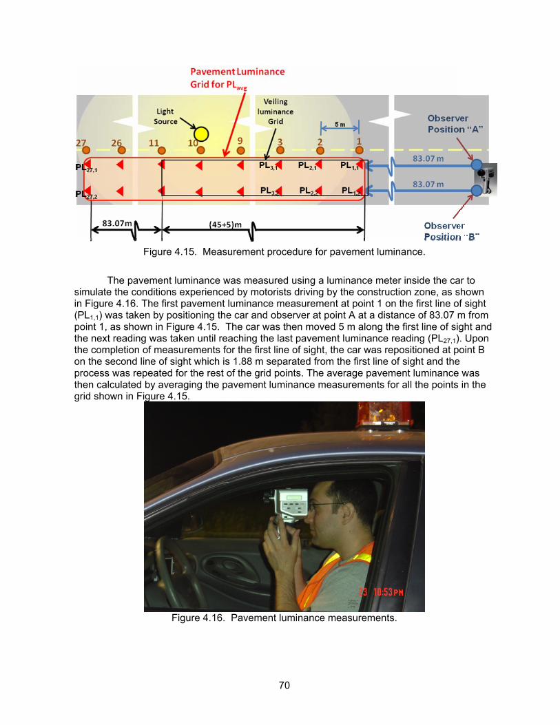
70
Figure 4.15. Measurement procedure for pavement luminance.
The pavement luminance was measured using a luminance meter inside the car to simulate the conditions experienced by motorists driving by the construction zone, as shown in Figure 4.16. The first pavement luminance measurement at point 1 on the first line of sight (PL1,1) was taken by positioning the car and observer at point A at a distance of 83.07 m from point 1, as shown in Figure 4.15. The car was then moved 5 m along the first line of sight and the next reading was taken until reaching the last pavement luminance reading (PL27,1). Upon the completion of measurements for the first line of sight, the car was repositioned at point B on the second line of sight which is 1.88 m separated from the first line of sight and the process was repeated for the rest of the grid points. The average pavement luminance was then calculated by averaging the pavement luminance measurements for all the points in the grid shown in Figure 4.15.
Figure 4.16. Pavement luminance measurements.
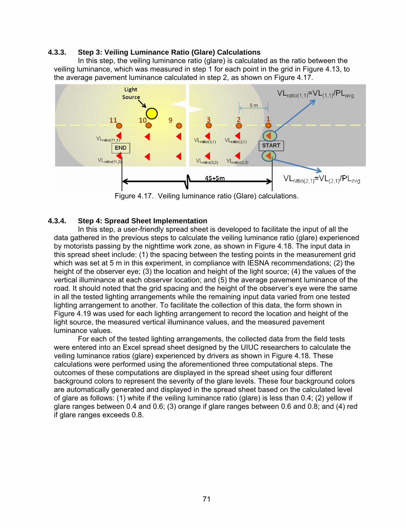
71
4.3.3. Step 3: Veiling Luminance Ratio (Glare) Calculations In this step, the veiling luminance ratio (glare) is calculated as the ratio between the veiling luminance, which was measured in step 1 for each point in the grid in Figure 4.13, to the average pavement luminance calculated in step 2, as shown on Figure 4.17.
Figure 4.17. Veiling luminance ratio (Glare) calculations.
4.3.4. Step 4: Spread Sheet Implementation In this step, a user-friendly spread sheet is developed to facilitate the input of all the data gathered in the previous steps to calculate the veiling luminance ratio (glare) experienced by motorists passing by the nighttime work zone, as shown in Figure 4.18. The input data in this spread sheet include: (1) the spacing between the testing points in the measurement grid which was set at 5 m in this experiment, in compliance with IESNA recommendations; (2) the height of the observer eye; (3) the location and height of the light source; (4) the values of the vertical illuminance at each observer location; and (5) the average pavement luminance of the road. It should noted that the grid spacing and the height of the observer’s eye were the same in all the tested lighting arrangements while the remaining input data varied from one tested lighting arrangement to another. To facilitate the collection of this data, the form shown in Figure 4.19 was used for each lighting arrangement to record the location and height of the light source, the measured vertical illuminance values, and the measured pavement luminance values. For each of the tested lighting arrangements, the collected data from the field tests were entered into an Excel spread sheet designed by the UIUC researchers to calculate the veiling luminance ratios (glare) experienced by drivers as shown in Figure 4.18. These calculations were performed using the aforementioned three computational steps. The outcomes of these computations are displayed in the spread sheet using four different background colors to represent the severity of the glare levels. These four background colors are automatically generated and displayed in the spread sheet based on the calculated level of glare as follows: (1) white if the veiling luminance ratio (glare) is less than 0.4; (2) yellow if glare ranges between 0.4 and 0.6; (3) orange if glare ranges between 0.6 and 0.8; and (4) red if glare ranges exceeds 0.8.

72
5
1.45
1
Light # x y z
1 1.92 45 4.5
0.988333333
Values Entered11
0.7 0.00 0.230.95 5.00 0.261.3 10.00 0.281.85 15.00 0.302.75 20.00 0.324.45 25.00 0.358.75 30.00 0.4119.8 35.00 0.452.25 40.00 0.023.25 45.00 0.001.8 50.00 0.00
Insert the space between the locations:
Insert the height of the observer:
Number of light sources entered:
Average Pavement Luminance:
Vertical Illuminance Observer Location Glare
Glare Calculations
Figure 4.18. Spread sheet implementation.
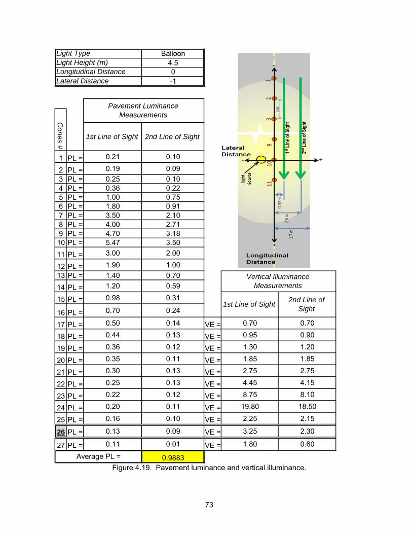
73
Balloon4.50-1
1st Line of Sight 2nd Line of Sight
1 PL = 0.21 0.10
2 PL = 0.19 0.093 PL = 0.25 0.104 PL = 0.36 0.225 PL = 1.00 0.756 PL = 1.80 0.917 PL = 3.50 2.108 PL = 4.00 2.719 PL = 4.70 3.18
10 PL = 5.47 3.5011 PL = 3.00 2.00
12 PL = 1.90 1.0013 PL = 1.40 0.7014 PL = 1.20 0.59
15 PL = 0.98 0.31
16 PL = 0.70 0.24
17 PL = 0.50 0.14 VE = 0.70 0.70
18 PL = 0.44 0.13 VE = 0.95 0.90
19 PL = 0.36 0.12 VE = 1.30 1.20
20 PL = 0.35 0.11 VE = 1.85 1.85
21 PL = 0.30 0.13 VE = 2.75 2.75
22 PL = 0.25 0.13 VE = 4.45 4.15
23 PL = 0.22 0.12 VE = 8.75 8.10
24 PL = 0.20 0.11 VE = 19.80 18.50
25 PL = 0.16 0.10 VE = 2.25 2.15
26 PL = 0.13 0.09 VE = 3.25 2.30
27 PL = 0.11 0.01 VE = 1.80 0.60
0.9883
Light TypeLight Height (m)
Lateral Distance
Average PL =
Longitudinal Distance
1st Line of Sight 2nd Line of Sight
Vertical Illuminance Measurements
Cones #
Pavement Luminance Measurements
Figure 4.19. Pavement luminance and vertical illuminance.

74
4.4. Horizontal Illuminance and Uniformity Ratio Measurements Procedure In addition to measuring and calculating the veiling luminance ratio in the previous section, the horizontal illuminance provided by the tested lighting arrangements was also measured and calculated. The purpose of this calculation is to evaluate the lighting performance (i.e., average horizontal illuminance and lighting uniformity) as well as the veiling luminance ratio for all the tested lighting arrangements. The horizontal illuminance (HI) was measured using an illuminance meter (see Figure 4.20) at each measurement point on the grid shown in Figure 4.21. The measurement points in this grid were located along the two quarter lane lines in the simulated work zone and extended 20 m on both sides of the light source with a spacing of 5 m according to recommendations from IESNA (IESNA 2004). To facilitate the collection of this measurement data, the form shown in Figure 4.22 was used for each lighting arrangement to record the measured horizontal illuminance values for each point in the utilized grid.
Figure 4.20. Horizontal illuminance measurements.
Figure 4.21. Horizontal illuminance measurements.

75
2.8 m 0.92 m1 -20 1.61 1.632 -15 3.85 43 -10 12.5 13.14 -5 55 665 0 220 2806 5 55 667 10 12.5 13.18 15 3.85 49 20 1.61 1.63
HI-Distribution Table (in lux)Work Area
Meas. Points
Distance (m
)
Figure 4.22. Horizontal illuminance distribution (in lux).
The average horizontal illuminance (Eavg) was calculated by dividing the total accumulated illuminance (Etotal) in all the grid points in the specified work area by the number of points (P) in that grid, as shown in Equation 4.1. For each tested lighting arrangement, the average horizontal illuminance was calculated for three possible scenarios of work areas with a length of 20 m, 30 m, or 40 m, as shown in Figure 4.21. These lengths were selected to represent the typical work areas on both sides of the light source that were observed during the site visits and/or the spacing between equally spaced light sources along the length of the work zone.
PEE total
avg = (4.1)
Where, Etotal = accumulated illuminance in all grid points (P) in the construction work area (in lux);
and P = total number of the points in the grid in the work zone.
The lighting uniformity ratio (U) is represented by the ratio between the previously calculated average illuminance in the work area (Eavg) and the minimum illuminance measured at any grid point in the work zone as shown in Equation 4.2. It should be noted that lighting uniformity improves on construction zones when the value of the uniformity ratio decreases, which indicates smaller differences between the darkest point and the average illuminance in the work area.
minEE
U avg= (4.2)
Where, Eavg = average horizontal illuminance in the work area (in lux); and
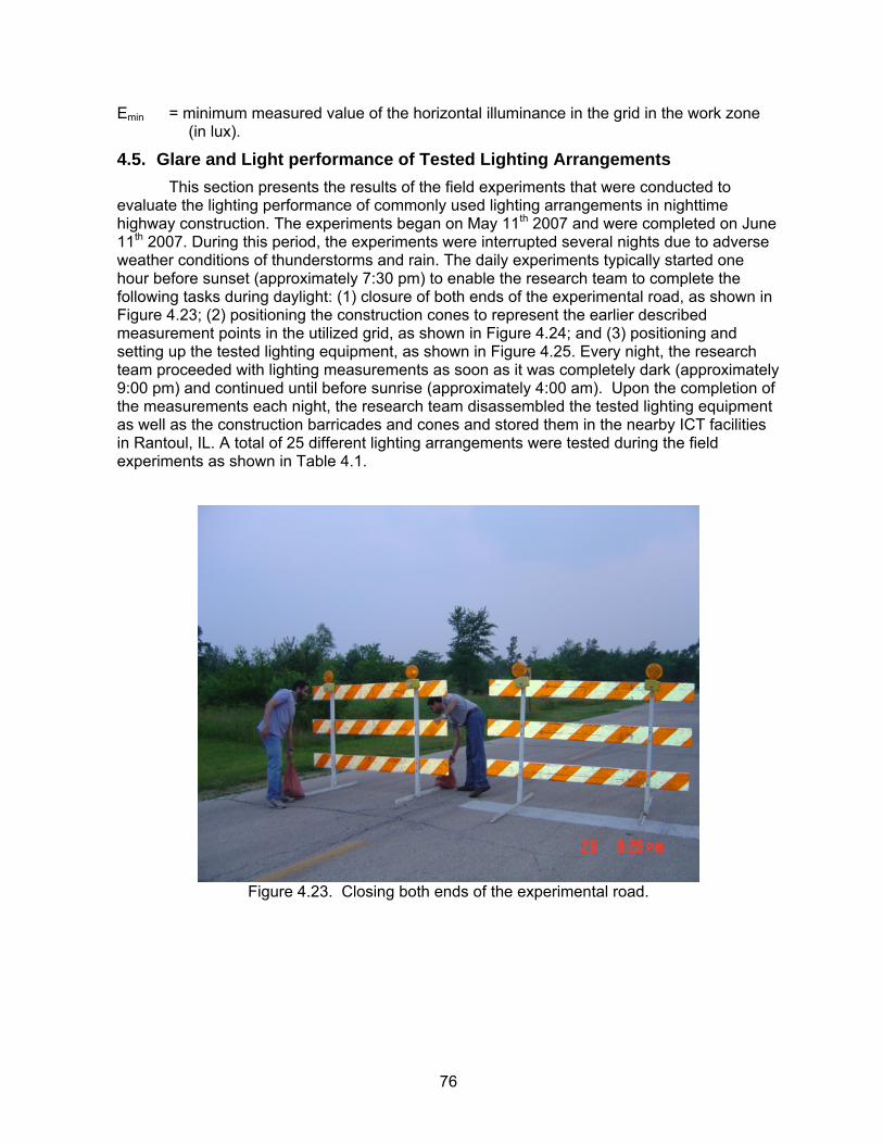
76
Emin = minimum measured value of the horizontal illuminance in the grid in the work zone (in lux).
4.5. Glare and Light performance of Tested Lighting Arrangements This section presents the results of the field experiments that were conducted to evaluate the lighting performance of commonly used lighting arrangements in nighttime highway construction. The experiments began on May 11th 2007 and were completed on June 11th 2007. During this period, the experiments were interrupted several nights due to adverse weather conditions of thunderstorms and rain. The daily experiments typically started one hour before sunset (approximately 7:30 pm) to enable the research team to complete the following tasks during daylight: (1) closure of both ends of the experimental road, as shown in Figure 4.23; (2) positioning the construction cones to represent the earlier described measurement points in the utilized grid, as shown in Figure 4.24; and (3) positioning and setting up the tested lighting equipment, as shown in Figure 4.25. Every night, the research team proceeded with lighting measurements as soon as it was completely dark (approximately 9:00 pm) and continued until before sunrise (approximately 4:00 am). Upon the completion of the measurements each night, the research team disassembled the tested lighting equipment as well as the construction barricades and cones and stored them in the nearby ICT facilities in Rantoul, IL. A total of 25 different lighting arrangements were tested during the field experiments as shown in Table 4.1.
Figure 4.23. Closing both ends of the experimental road.
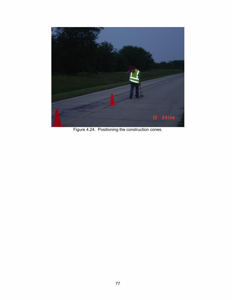
77
Figure 4.24. Positioning the construction cones.
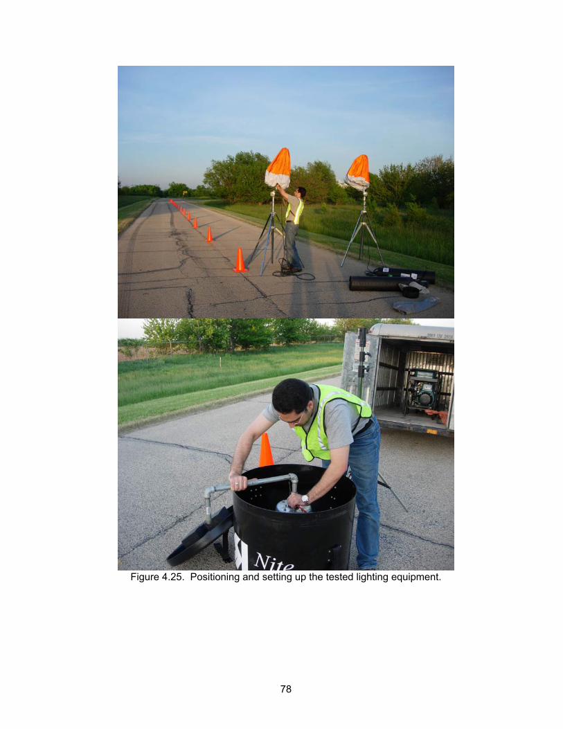
78
Figure 4.25. Positioning and setting up the tested lighting equipment.
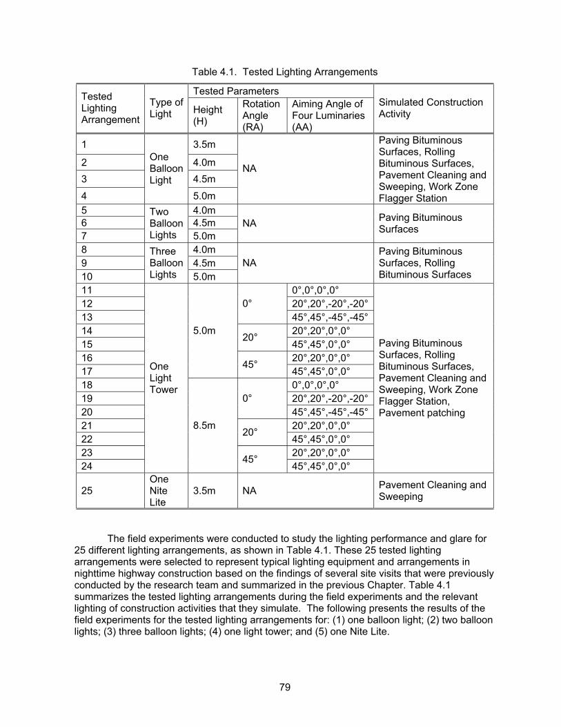
79
Table 4.1. Tested Lighting Arrangements
Tested Parameters Tested Lighting Arrangement
Type of Light Height
(H)
Rotation Angle (RA)
Aiming Angle of Four Luminaries (AA)
Simulated Construction Activity
1 3.5m
2 4.0m 3 4.5m
4
One Balloon Light
5.0m
NA
Paving Bituminous Surfaces, Rolling Bituminous Surfaces, Pavement Cleaning and Sweeping, Work Zone Flagger Station
5 4.0m 6 4.5m 7
Two Balloon Lights 5.0m
NA Paving Bituminous Surfaces
8 4.0m 9 4.5m 10
Three Balloon Lights 5.0m
NA Paving Bituminous Surfaces, Rolling Bituminous Surfaces
11 0°,0°,0°,0° 12 20°,20°,-20°,-20°13
0° 45°,45°,-45°,-45°
14 20°,20°,0°,0° 15
20° 45°,45°,0°,0°
16 20°,20°,0°,0° 17
5.0m
45° 45°,45°,0°,0°
18 0°,0°,0°,0° 19 20°,20°,-20°,-20°20
0° 45°,45°,-45°,-45°
21 20°,20°,0°,0° 22
20° 45°,45°,0°,0°
23 20°,20°,0°,0° 24
One Light Tower
8.5m
45° 45°,45°,0°,0°
Paving Bituminous Surfaces, Rolling Bituminous Surfaces, Pavement Cleaning and Sweeping, Work Zone Flagger Station, Pavement patching
25 One Nite Lite
3.5m NA Pavement Cleaning and Sweeping
The field experiments were conducted to study the lighting performance and glare for 25 different lighting arrangements, as shown in Table 4.1. These 25 tested lighting arrangements were selected to represent typical lighting equipment and arrangements in nighttime highway construction based on the findings of several site visits that were previously conducted by the research team and summarized in the previous Chapter. Table 4.1 summarizes the tested lighting arrangements during the field experiments and the relevant lighting of construction activities that they simulate. The following presents the results of the field experiments for the tested lighting arrangements for: (1) one balloon light; (2) two balloon lights; (3) three balloon lights; (4) one light tower; and (5) one Nite Lite.
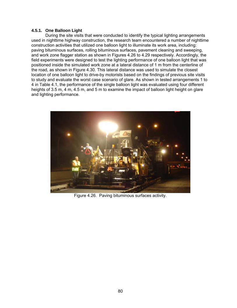
80
4.5.1. One Balloon Light During the site visits that were conducted to identify the typical lighting arrangements used in nighttime highway construction, the research team encountered a number of nighttime construction activities that utilized one balloon light to illuminate its work area, including: paving bituminous surfaces, rolling bituminous surfaces, pavement cleaning and sweeping, and work zone flagger station as shown in Figures 4.26 to 4.29 respectively. Accordingly, the field experiments were designed to test the lighting performance of one balloon light that was positioned inside the simulated work zone at a lateral distance of 1 m from the centerline of the road, as shown in Figure 4.30. This lateral distance was used to simulate the closest location of one balloon light to drive-by motorists based on the findings of previous site visits to study and evaluate the worst case scenario of glare. As shown in tested arrangements 1 to 4 in Table 4.1, the performance of the single balloon light was evaluated using four different heights of 3.5 m, 4 m, 4.5 m, and 5 m to examine the impact of balloon light height on glare and lighting performance.
Figure 4.26. Paving bituminous surfaces activity.
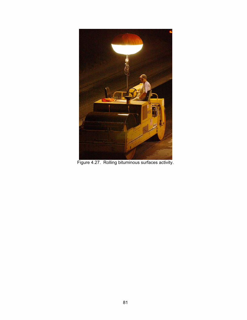
81
Figure 4.27. Rolling bituminous surfaces activity.
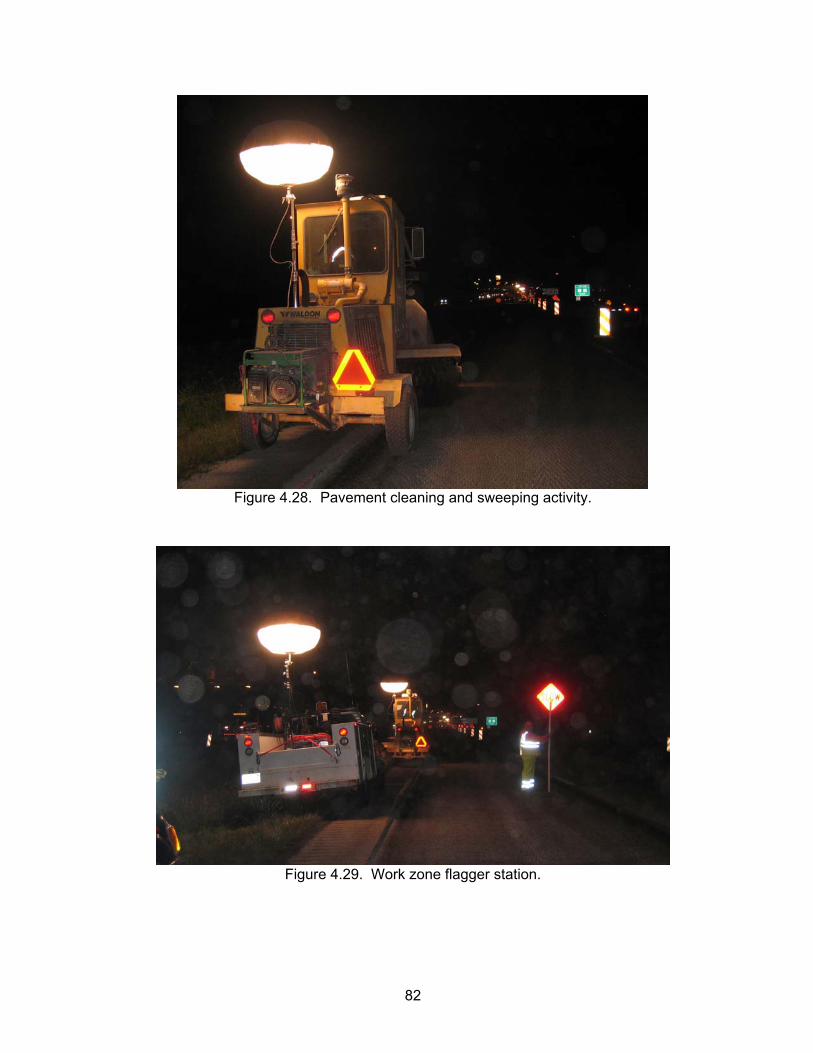
82
Figure 4.28. Pavement cleaning and sweeping activity.
Figure 4.29. Work zone flagger station.
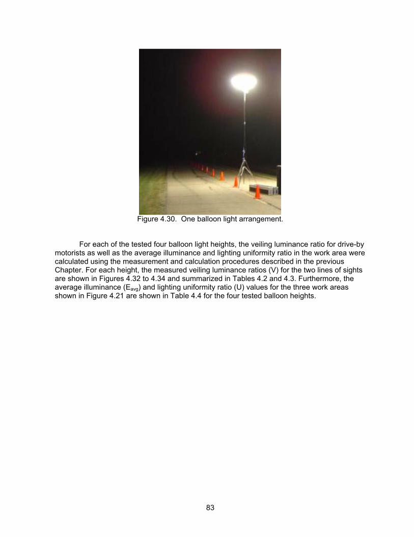
83
Figure 4.30. One balloon light arrangement.
For each of the tested four balloon light heights, the veiling luminance ratio for drive-by motorists as well as the average illuminance and lighting uniformity ratio in the work area were calculated using the measurement and calculation procedures described in the previous Chapter. For each height, the measured veiling luminance ratios (V) for the two lines of sights are shown in Figures 4.32 to 4.34 and summarized in Tables 4.2 and 4.3. Furthermore, the average illuminance (Eavg) and lighting uniformity ratio (U) values for the three work areas shown in Figure 4.21 are shown in Table 4.4 for the four tested balloon heights.
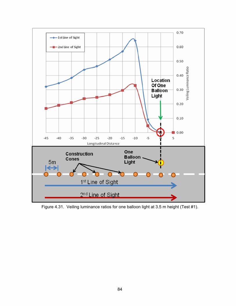
84
Figure 4.31. Veiling luminance ratios for one balloon light at 3.5 m height (Test #1).
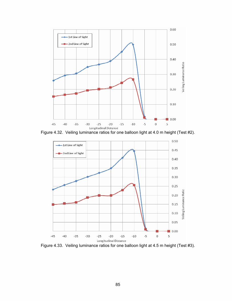
85
Figure 4.32. Veiling luminance ratios for one balloon light at 4.0 m height (Test #2).
Figure 4.33. Veiling luminance ratios for one balloon light at 4.5 m height (Test #3).
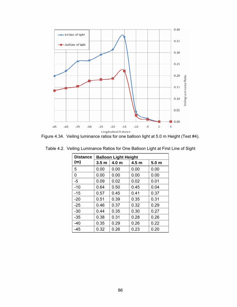
86
Figure 4.34. Veiling luminance ratios for one balloon light at 5.0 m Height (Test #4).
Table 4.2. Veiling Luminance Ratios for One Balloon Light at First Line of Sight
Balloon Light Height Distance (m) 3.5 m 4.0 m 4.5 m 5.0 m 5 0.00 0.00 0.00 0.00 0 0.00 0.00 0.00 0.00 -5 0.09 0.02 0.02 0.01 -10 0.64 0.50 0.45 0.04 -15 0.57 0.45 0.41 0.37 -20 0.51 0.39 0.35 0.31 -25 0.46 0.37 0.32 0.29 -30 0.44 0.35 0.30 0.27 -35 0.38 0.31 0.28 0.26 -40 0.35 0.29 0.26 0.22 -45 0.32 0.26 0.23 0.20

87
Table 4.3. Veiling Luminance Ratios for One Balloon Light at Second Line of Sight
Balloon Light Height Distance (m) 3.5 m 4.0 m 4.5 m 5.0 m 5 0.00 0.00 0.00 0.00 0 0.00 0.00 0.00 0.00 -5 0.05 0.01 0.01 0.01 -10 0.33 0.27 0.26 0.03 -15 0.30 0.24 0.23 0.22 -20 0.26 0.21 0.20 0.19 -25 0.25 0.20 0.20 0.18 -30 0.24 0.19 0.19 0.18 -35 0.21 0.17 0.16 0.15 -40 0.19 0.16 0.15 0.15 -45 0.17 0.15 0.15 0.14
Table 4.4. Average Horizontal Illuminance and Lighting Uniformity Ratios for One Balloon Light
Balloon Light Height in meters (H)
Work Area Length in meters
Average Horizontal Illuminance in lux (Eavg)
Lighting Uniformity Ratio (U)
20 85.79 10.55
30 61.96 26.94 3.5
40 48.44 44.44
20 85.52 7.64
30 62.10 17.74 4.0
40 48.64 32.43
20 79.32 6.35
30 57.78 15.01 4.5
40 45.30 28.14
20 70.50 5.11
30 51.63 11.73 5.0
40 40.58 21.36

88
The main findings of the above four tested lighting arrangements for a single balloon light includes: (1) Veiling luminance ratio/glare steadily increases for drive by motorists as they approach
the light source and it reaches a peak at 10 m before the balloon light for the first three tested heights (3.5 m, 4 m, 4.5m) while the peak glare value for the fourth tested height (5 m) was observed at 15 m before the light, as shown in Tables 4.2 and 4.3 and Figures 4.31 to 4.34.
(2) Veiling luminance ratios experienced at the first line of sight are consistently higher than those observed at the second line of sight, as shown in Figures 4.31 to 4.34. The increase in these ratios at the first line of sight compared to the second light of sight is due to the closer lateral distance to the light source (see Figure 4.31).
(3) For the second line of sight in all the tested balloon light heights, the veiling luminance ratios in all locations were less than 0.4 which is the maximum ratio allowed by IESNA for roadway lighting (IESNA 2004), as shown in Table 4.3.
(4) For the first line of sight in all the tested balloon light heights, the 0.4 veiling luminance ratio was exceeded in 9 of the 44 tested locations as follows:
4.1) For the tested height of 3.5 m, veiling luminance ratios exceeded 0.4 at five locations before the light source at 10 m, 15 m, 20 m, 25 m and 30 m, as shown in Table 4.2;
4.2) For the tested height of 4 m, veiling luminance ratios exceeded 0.4 at two locations at 10 m and 15 m before the light source, as shown in Table 4.2;
4.3) For the tested height of 4.5 m, veiling luminance ratios exceeded 0.4 at two locations at 10 m and 15 m before the light source, as shown in Table 4.2;
4.4) For the tested height of 5 m, veiling luminance ratios were consistently less than 0.4 in all locations, as shown in Table 4.2;
(5) Veiling luminance ratios steadily decrease as the balloon light height increases as shown in Tables 4.2 and 4.3.
(6) Average horizontal illuminance in the work area continues to decrease as the balloon light height increases as shown in Table 4.4.
(7) Lighting uniformity ratio in the work area steadily decreases as the balloon light height increases as shown in Table 4.4.
4.5.2. Two Balloon Lights During the site visits, the research team observed a number of nighttime highway construction projects in Illinois that utilized two balloon lights to provide lighting for paving bituminous surfaces activity, as shown in Figure 4.35. Accordingly, the field experiments were designed to test the lighting performance of two balloon lights that were positioned inside the simulated work zone and separated by 2.72 m to simulate the same lighting settings observed during the site visits, as shown in Figure 4.36. As shown in tested arrangements 5 to 7 in Table 4.1, the two balloon lights were tested using three different heights of 4 m, 4.5 m, and 5 m to examine the impact of height on glare and lighting performance.
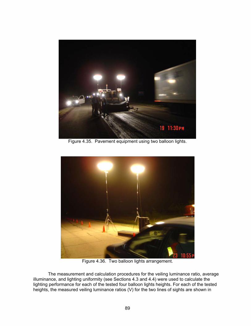
89
Figure 4.35. Pavement equipment using two balloon lights.
Figure 4.36. Two balloon lights arrangement.
The measurement and calculation procedures for the veiling luminance ratio, average illuminance, and lighting uniformity (see Sections 4.3 and 4.4) were used to calculate the lighting performance for each of the tested four balloon lights heights. For each of the tested heights, the measured veiling luminance ratios (V) for the two lines of sights are shown in

90
Figures 4.37 to 4.39 and in Tables 4.5 and 4.6. In addition, the average illuminance (Eavg) and lighting uniformity ratio (U) values for the three work areas shown in Figure 4.21 are shown in Table 4.7 for the tested balloon heights.
Figure 4.37. Veiling luminance ratios for two balloon lights at 4.0 m height (Test #5).
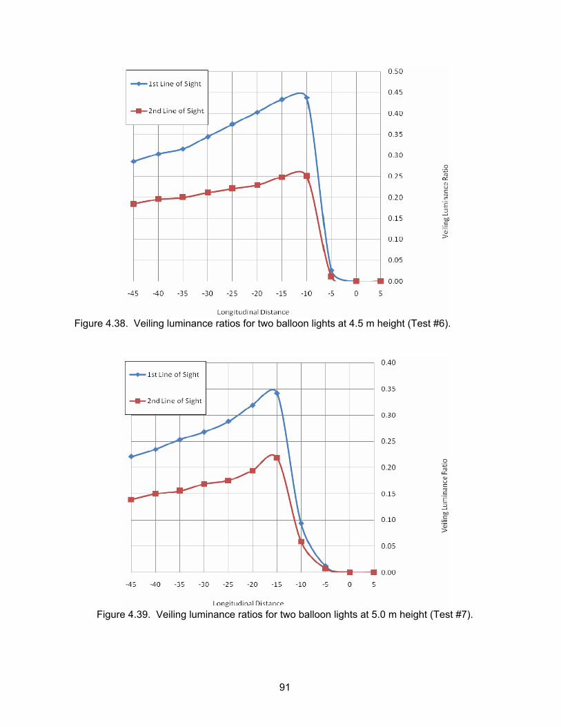
91
Figure 4.38. Veiling luminance ratios for two balloon lights at 4.5 m height (Test #6).
Figure 4.39. Veiling luminance ratios for two balloon lights at 5.0 m height (Test #7).
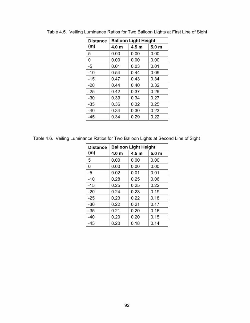
92
Table 4.5. Veiling Luminance Ratios for Two Balloon Lights at First Line of Sight
Balloon Light Height Distance (m) 4.0 m 4.5 m 5.0 m 5 0.00 0.00 0.00 0 0.00 0.00 0.00 -5 0.01 0.03 0.01 -10 0.54 0.44 0.09 -15 0.47 0.43 0.34 -20 0.44 0.40 0.32 -25 0.42 0.37 0.29 -30 0.39 0.34 0.27 -35 0.36 0.32 0.25 -40 0.34 0.30 0.23 -45 0.34 0.29 0.22
Table 4.6. Veiling Luminance Ratios for Two Balloon Lights at Second Line of Sight
Balloon Light Height Distance (m) 4.0 m 4.5 m 5.0 m 5 0.00 0.00 0.00 0 0.00 0.00 0.00 -5 0.02 0.01 0.01 -10 0.28 0.25 0.06 -15 0.25 0.25 0.22 -20 0.24 0.23 0.19 -25 0.23 0.22 0.18 -30 0.22 0.21 0.17 -35 0.21 0.20 0.16 -40 0.20 0.20 0.15 -45 0.20 0.18 0.14
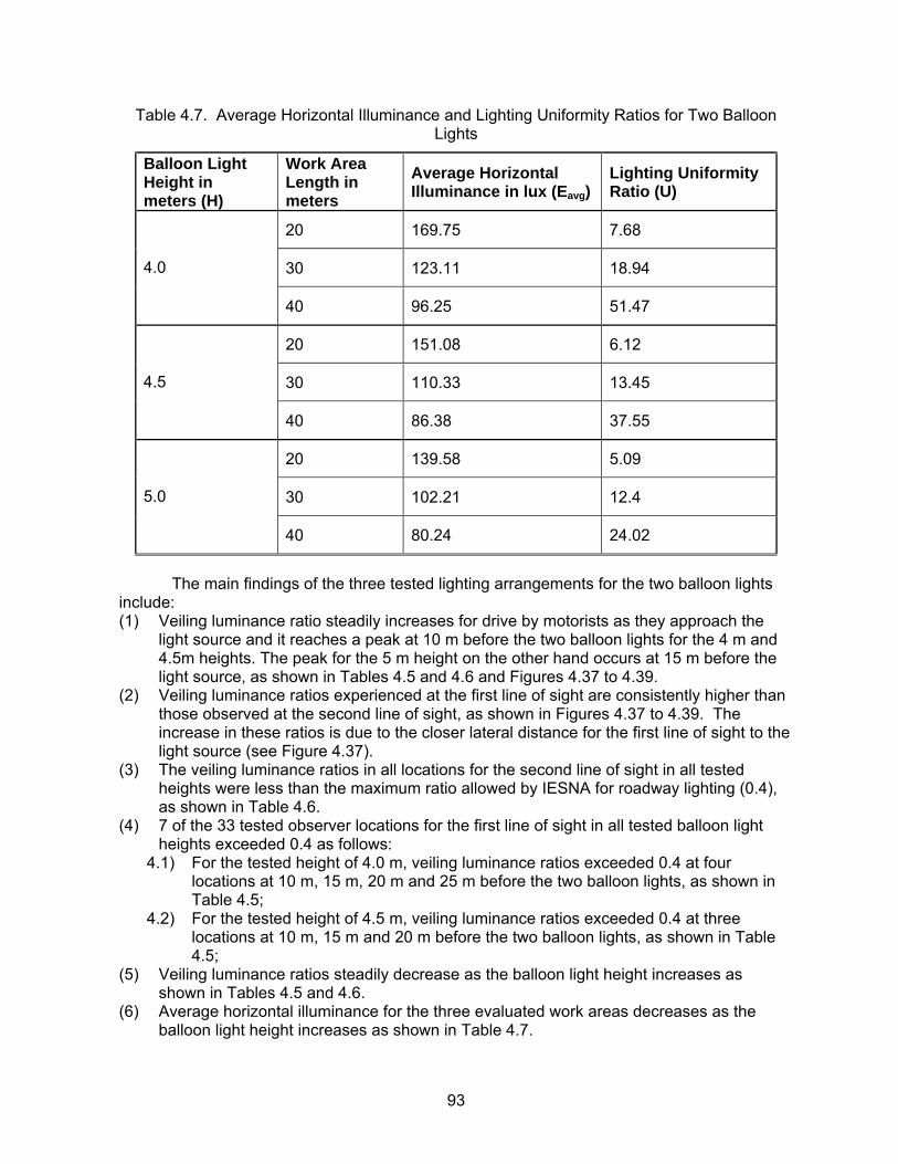
93
Table 4.7. Average Horizontal Illuminance and Lighting Uniformity Ratios for Two Balloon Lights
Balloon Light Height in meters (H)
Work Area Length in meters
Average Horizontal Illuminance in lux (Eavg)
Lighting Uniformity Ratio (U)
20 169.75 7.68
30 123.11 18.94 4.0
40 96.25 51.47
20 151.08 6.12
30 110.33 13.45 4.5
40 86.38 37.55
20 139.58 5.09
30 102.21 12.4 5.0
40 80.24 24.02
The main findings of the three tested lighting arrangements for the two balloon lights include: (1) Veiling luminance ratio steadily increases for drive by motorists as they approach the
light source and it reaches a peak at 10 m before the two balloon lights for the 4 m and 4.5m heights. The peak for the 5 m height on the other hand occurs at 15 m before the light source, as shown in Tables 4.5 and 4.6 and Figures 4.37 to 4.39.
(2) Veiling luminance ratios experienced at the first line of sight are consistently higher than those observed at the second line of sight, as shown in Figures 4.37 to 4.39. The increase in these ratios is due to the closer lateral distance for the first line of sight to the light source (see Figure 4.37).
(3) The veiling luminance ratios in all locations for the second line of sight in all tested heights were less than the maximum ratio allowed by IESNA for roadway lighting (0.4), as shown in Table 4.6.
(4) 7 of the 33 tested observer locations for the first line of sight in all tested balloon light heights exceeded 0.4 as follows:
4.1) For the tested height of 4.0 m, veiling luminance ratios exceeded 0.4 at four locations at 10 m, 15 m, 20 m and 25 m before the two balloon lights, as shown in Table 4.5;
4.2) For the tested height of 4.5 m, veiling luminance ratios exceeded 0.4 at three locations at 10 m, 15 m and 20 m before the two balloon lights, as shown in Table 4.5;
(5) Veiling luminance ratios steadily decrease as the balloon light height increases as shown in Tables 4.5 and 4.6.
(6) Average horizontal illuminance for the three evaluated work areas decreases as the balloon light height increases as shown in Table 4.7.

94
(7) Lighting uniformity ratio in the work area steadily decreases as the height of the two balloon lights increases as shown in Table 4.7.
4.5.3. Three Balloon Lights During the site visits, the research team observed in a number of projects the utilization of three balloon lights in close proximity to each other. In these projects, the paving equipment utilized two balloon lights on the sides of the paver while a nearby roller utilized a third balloon light, as shown in Figure 4.40. Accordingly, the field experiments were designed to test the veiling luminance ratio, average horizontal illuminance, and lighting uniformity for the three balloon lights. Two of the balloon lights were positioned inside the simulated work zone and separated by 2.72 m to simulate a paving bituminous surface activity while one balloon light was positioned in the middle of the simulated work zone to represent a rolling bituminous surface activity, as shown in Figure 4.41. The two balloon lights were positioned with a 10 m longitudinal distance away from the third balloon light to simulate the closest location of a paver to a roller in the simulated work zone. As shown in tested arrangements 8 to 10 in Table 4.1, the three balloon lights were tested using three different heights of 4 m, 4.5 m, and 5 m to examine the impact of height on the veiling luminance ratio, average horizontal illuminance, and lighting uniformity.
Figure 4.40. Utilization of three balloon lights in nighttime work zone.
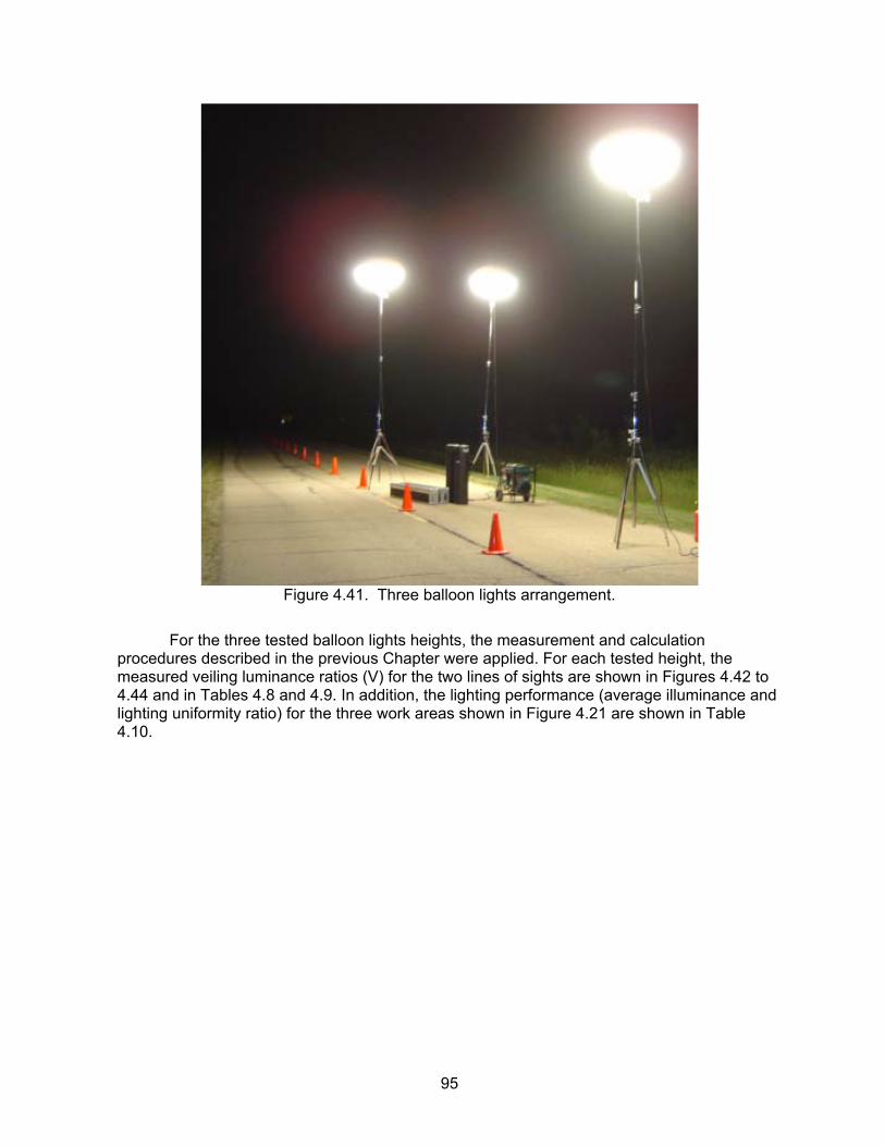
95
Figure 4.41. Three balloon lights arrangement.
For the three tested balloon lights heights, the measurement and calculation procedures described in the previous Chapter were applied. For each tested height, the measured veiling luminance ratios (V) for the two lines of sights are shown in Figures 4.42 to 4.44 and in Tables 4.8 and 4.9. In addition, the lighting performance (average illuminance and lighting uniformity ratio) for the three work areas shown in Figure 4.21 are shown in Table 4.10.
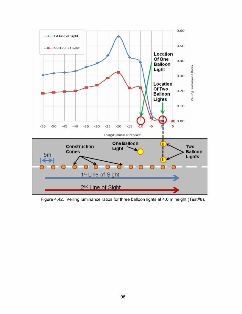
96
Figure 4.42. Veiling luminance ratios for three balloon lights at 4.0 m height (Test#8).
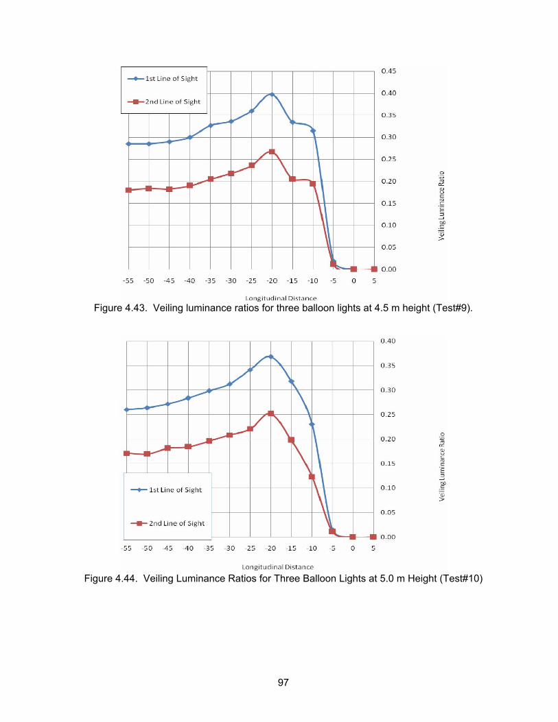
97
Figure 4.43. Veiling luminance ratios for three balloon lights at 4.5 m height (Test#9).
Figure 4.44. Veiling Luminance Ratios for Three Balloon Lights at 5.0 m Height (Test#10)

98
Table 4.8. Veiling Luminance Ratios for Three Balloon Lights at First Line of Sight
Balloon Light Height Distance (m) 4.0 m 4.5 m 5.0 m 5 0.00 0.00 0.00 0 0.00 0.00 0.00 -5 0.05 0.02 0.01 -10 0.39 0.31 0.23 -15 0.42 0.33 0.32 -20 0.56 0.40 0.37 -25 0.44 0.36 0.34 -30 0.39 0.34 0.31 -35 0.36 0.33 0.30 -40 0.33 0.30 0.28 -45 0.32 0.29 0.27 -50 0.32 0.29 0.26 -55 0.31 0.29 0.26
Table 4.9. Veiling Luminance Ratios for Three Balloon Lights at Second Line of Sight
Balloon Light Height Distance (m) 4.0 m 4.5 m 5.0 m 5 0.00 0.00 0.00 0 0.00 0.00 0.00 -5 0.02 0.01 0.01 -10 0.22 0.19 0.12 -15 0.22 0.20 0.20 -20 0.32 0.27 0.25 -25 0.29 0.24 0.22 -30 0.24 0.22 0.21 -35 0.22 0.20 0.20 -40 0.20 0.19 0.18 -45 0.20 0.18 0.18 -50 0.19 0.18 0.17 -55 0.18 0.18 0.17
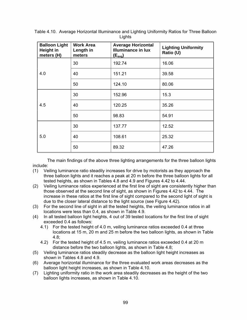
99
Table 4.10. Average Horizontal Illuminance and Lighting Uniformity Ratios for Three Balloon Lights
Balloon Light Height in meters (H)
Work Area Length in meters
Average Horizontal Illuminance in lux (Eavg)
Lighting Uniformity Ratio (U)
30 192.74 16.06
40 151.21 39.58 4.0
50 124.10 80.06
30 152.96 15.3
40 120.25 35.26 4.5
50 98.83 54.91
30 137.77 12.52
40 108.61 25.32 5.0
50 89.32 47.26
The main findings of the above three lighting arrangements for the three balloon lights include: (1) Veiling luminance ratio steadily increases for drive by motorists as they approach the
three balloon lights and it reaches a peak at 20 m before the three balloon lights for all tested heights, as shown in Tables 4.8 and 4.9 and Figures 4.42 to 4.44.
(2) Veiling luminance ratios experienced at the first line of sight are consistently higher than those observed at the second line of sight, as shown in Figures 4.42 to 4.44. The increase in these ratios at the first line of sight compared to the second light of sight is due to the closer lateral distance to the light source (see Figure 4.42).
(3) For the second line of sight in all the tested heights, the veiling luminance ratios in all locations were less than 0.4, as shown in Table 4.9.
(4) In all tested balloon light heights, 4 out of 39 tested locations for the first line of sight exceeded 0.4 as follows:
4.1) For the tested height of 4.0 m, veiling luminance ratios exceeded 0.4 at three locations at 15 m, 20 m and 25 m before the two balloon lights, as shown in Table 4.8;
4.2) For the tested height of 4.5 m, veiling luminance ratios exceeded 0.4 at 20 m distance before the two balloon lights, as shown in Table 4.8;
(5) Veiling luminance ratios steadily decrease as the balloon light height increases as shown in Tables 4.8 and 4.9.
(6) Average horizontal illuminance for the three evaluated work areas decreases as the balloon light height increases, as shown in Table 4.10.
(7) Lighting uniformity ratio in the work area steadily decreases as the height of the two balloon lights increases, as shown in Table 4.10.
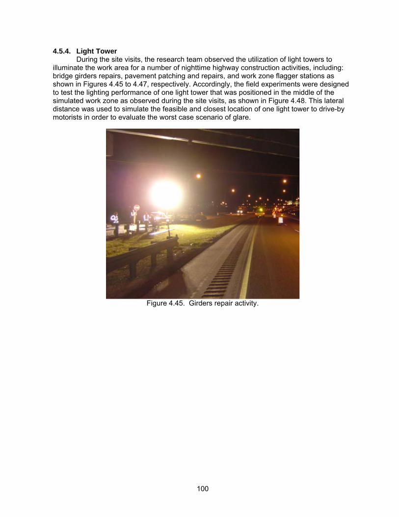
100
4.5.4. Light Tower During the site visits, the research team observed the utilization of light towers to illuminate the work area for a number of nighttime highway construction activities, including: bridge girders repairs, pavement patching and repairs, and work zone flagger stations as shown in Figures 4.45 to 4.47, respectively. Accordingly, the field experiments were designed to test the lighting performance of one light tower that was positioned in the middle of the simulated work zone as observed during the site visits, as shown in Figure 4.48. This lateral distance was used to simulate the feasible and closest location of one light tower to drive-by motorists in order to evaluate the worst case scenario of glare.
Figure 4.45. Girders repair activity.
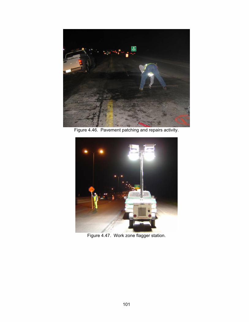
101
Figure 4.46. Pavement patching and repairs activity.
Figure 4.47. Work zone flagger station.

102
Figure 4.48. One light tower arrangement.
Moreover, the light tower was tested to examine the impact of three different parameters on the veiling luminance ratio and lighting performance. The tested parameters include: (1) the height of the light tower (H) which represents the vertical distance between the center of the luminaries and the road surface; (2) the rotation angle (RA) of the light tower which represents the rotation of the light tower pole around a vertical axis; and (3) the aiming angles (AA) of the four luminaries that denotes the vertical angle between the center of the beam spread of the luminaire and the nadir, as shown in Figure 4.49. These tested lighting arrangements are shown in Table 4.11.
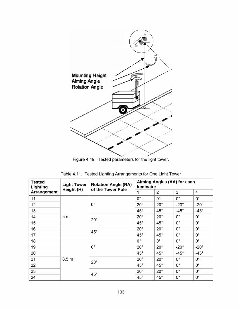
103
Figure 4.49. Tested parameters for the light tower.
Table 4.11. Tested Lighting Arrangements for One Light Tower
Aiming Angles (AA) for each luminaire
Tested Lighting Arrangement
Light Tower Height (H)
Rotation Angle (RA) of the Tower Pole 1 2 3 4
11 0° 0° 0° 0° 12 20° 20° -20° -20° 13
0° 45° 45° -45° -45°
14 20° 20° 0° 0° 15
20° 45° 45° 0° 0°
16 20° 20° 0° 0° 17
5 m
45° 45° 45° 0° 0°
18 0° 0° 0° 0° 19 20° 20° -20° -20° 20
0° 45° 45° -45° -45°
21 20° 20° 0° 0° 22
20° 45° 45° 0° 0°
23 20° 20° 0° 0° 24
8.5 m
45° 45° 45° 0° 0°
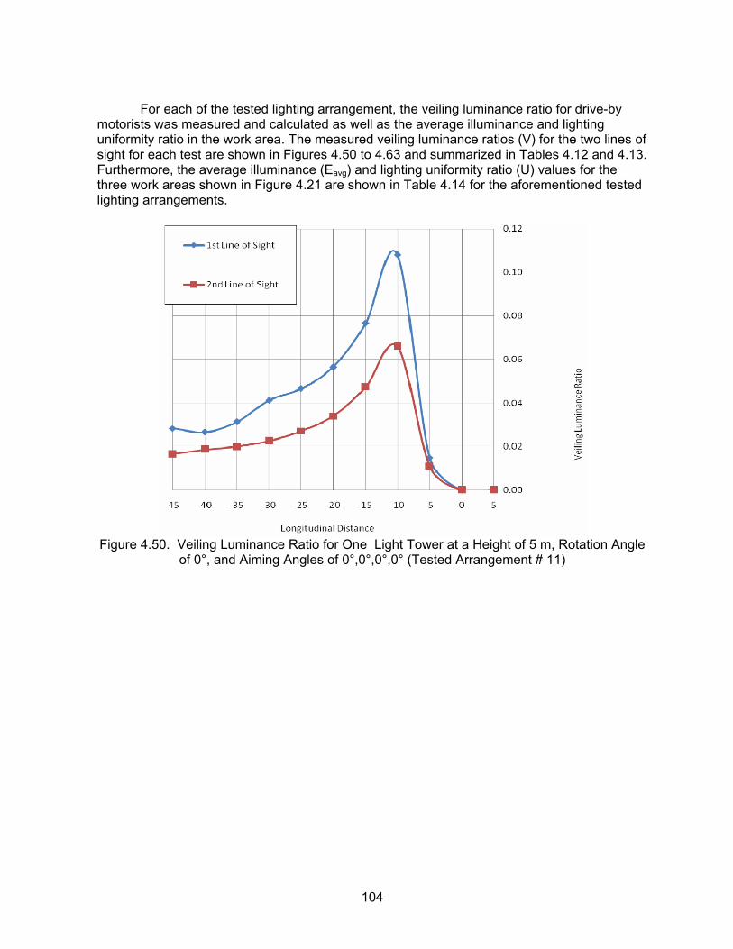
104
For each of the tested lighting arrangement, the veiling luminance ratio for drive-by motorists was measured and calculated as well as the average illuminance and lighting uniformity ratio in the work area. The measured veiling luminance ratios (V) for the two lines of sight for each test are shown in Figures 4.50 to 4.63 and summarized in Tables 4.12 and 4.13. Furthermore, the average illuminance (Eavg) and lighting uniformity ratio (U) values for the three work areas shown in Figure 4.21 are shown in Table 4.14 for the aforementioned tested lighting arrangements.
Figure 4.50. Veiling Luminance Ratio for One Light Tower at a Height of 5 m, Rotation Angle
of 0°, and Aiming Angles of 0°,0°,0°,0° (Tested Arrangement # 11)

105
Figure 4.51. Veiling luminance ratio for one light tower at a height of 8.5 m, rotation angle of
0°, and aiming angles of 0°,0°,0°,0° (Test #18).
Figure 4.52. Veiling luminance ratio for one light tower at a height of 5 m, rotation angle of 0°,
and aiming angles of 20°,20°,-20°,-20° (Test #12).
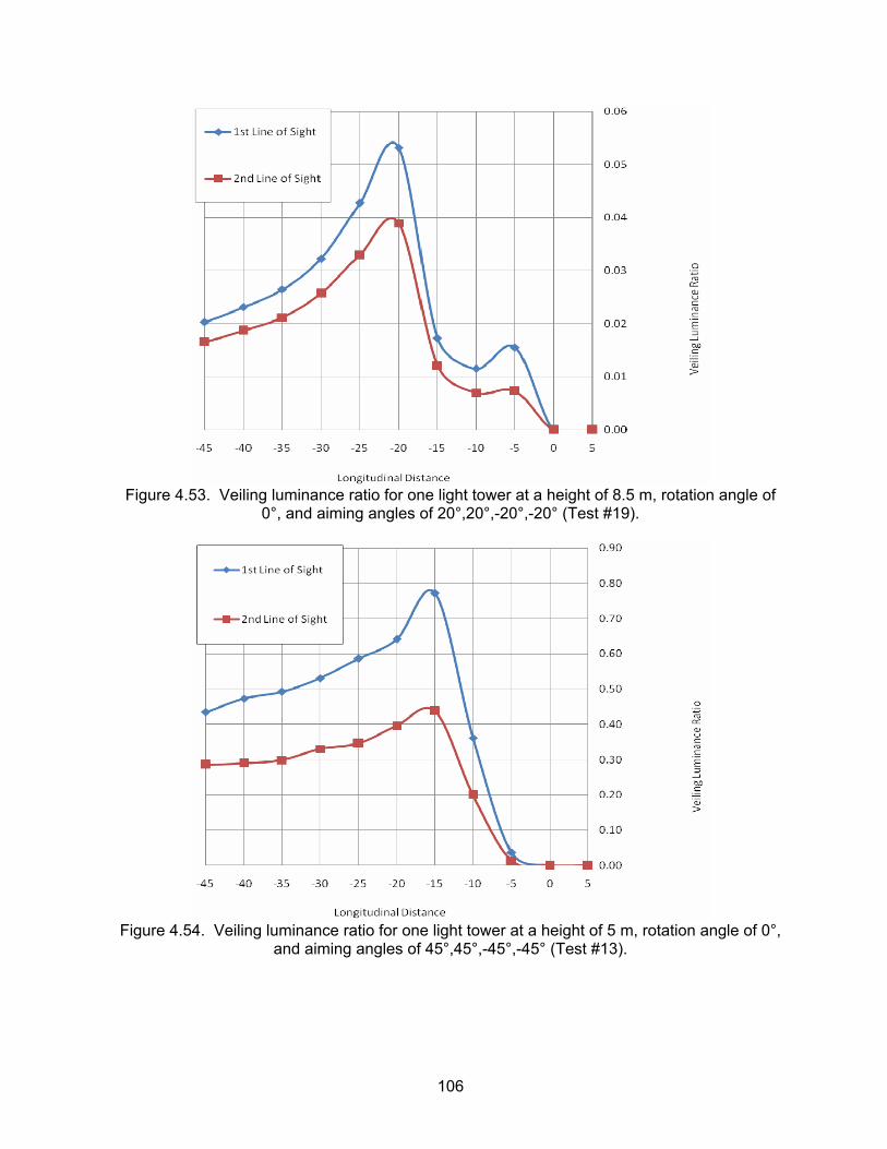
106
Figure 4.53. Veiling luminance ratio for one light tower at a height of 8.5 m, rotation angle of
0°, and aiming angles of 20°,20°,-20°,-20° (Test #19).
Figure 4.54. Veiling luminance ratio for one light tower at a height of 5 m, rotation angle of 0°,
and aiming angles of 45°,45°,-45°,-45° (Test #13).

107
Figure 4.55. Veiling luminance ratio for one light tower at a height of 8.5 m, rotation angle of
0°, and aiming angles of 45°,45°,-45°,-45° (Test #20).
Figure 4.56. Veiling luminance ratio for one light tower at a height of 5 m, rotation angle of
20°, and aiming angles of 20°,20°,0°,0° (Test #14).

108
Figure 4.57. Veiling luminance ratio for one light tower at a height of 8.5 m, rotation angle of
20°, and aiming angles of 20°,20°,0°,0° (Test #21).
Figure 4.58. Veiling luminance ratio for one light tower at a height of 5 m, rotation angle of
20°, and aiming angles of 45°,45°,0°,0° (Test #15).
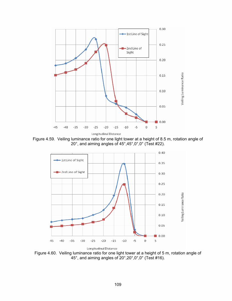
109
Figure 4.59. Veiling luminance ratio for one light tower at a height of 8.5 m, rotation angle of
20°, and aiming angles of 45°,45°,0°,0° (Test #22).
Figure 4.60. Veiling luminance ratio for one light tower at a height of 5 m, rotation angle of
45°, and aiming angles of 20°,20°,0°,0° (Test #16).

110
Figure 4.61. Veiling luminance ratio for one light tower at a height of 8.5 m, rotation angle of
45°, and aiming angles of 20°,20°,0°,0° (Test #23).
Figure 4.62. Veiling luminance ratio for one light tower at a height of 5 m, rotation angle of
45°, and aiming angles of 45°,45°,0°,0° (Test #17).
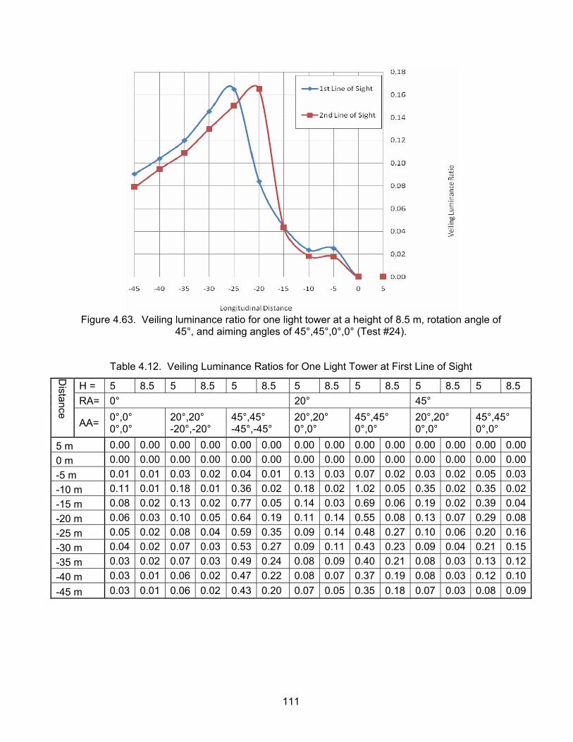
111
Figure 4.63. Veiling luminance ratio for one light tower at a height of 8.5 m, rotation angle of
45°, and aiming angles of 45°,45°,0°,0° (Test #24).
Table 4.12. Veiling Luminance Ratios for One Light Tower at First Line of Sight
H = 5 8.5 5 8.5 5 8.5 5 8.5 5 8.5 5 8.5 5 8.5 RA= 0° 20° 45°
Distance
AA= 0°,0° 0°,0°
20°,20° -20°,-20°
45°,45° -45°,-45°
20°,20° 0°,0°
45°,45° 0°,0°
20°,20° 0°,0°
45°,45° 0°,0°
5 m 0.00 0.00 0.00 0.00 0.00 0.00 0.00 0.00 0.00 0.00 0.00 0.00 0.00 0.000 m 0.00 0.00 0.00 0.00 0.00 0.00 0.00 0.00 0.00 0.00 0.00 0.00 0.00 0.00-5 m 0.01 0.01 0.03 0.02 0.04 0.01 0.13 0.03 0.07 0.02 0.03 0.02 0.05 0.03-10 m 0.11 0.01 0.18 0.01 0.36 0.02 0.18 0.02 1.02 0.05 0.35 0.02 0.35 0.02-15 m 0.08 0.02 0.13 0.02 0.77 0.05 0.14 0.03 0.69 0.06 0.19 0.02 0.39 0.04-20 m 0.06 0.03 0.10 0.05 0.64 0.19 0.11 0.14 0.55 0.08 0.13 0.07 0.29 0.08-25 m 0.05 0.02 0.08 0.04 0.59 0.35 0.09 0.14 0.48 0.27 0.10 0.06 0.20 0.16-30 m 0.04 0.02 0.07 0.03 0.53 0.27 0.09 0.11 0.43 0.23 0.09 0.04 0.21 0.15-35 m 0.03 0.02 0.07 0.03 0.49 0.24 0.08 0.09 0.40 0.21 0.08 0.03 0.13 0.12-40 m 0.03 0.01 0.06 0.02 0.47 0.22 0.08 0.07 0.37 0.19 0.08 0.03 0.12 0.10-45 m 0.03 0.01 0.06 0.02 0.43 0.20 0.07 0.05 0.35 0.18 0.07 0.03 0.08 0.09
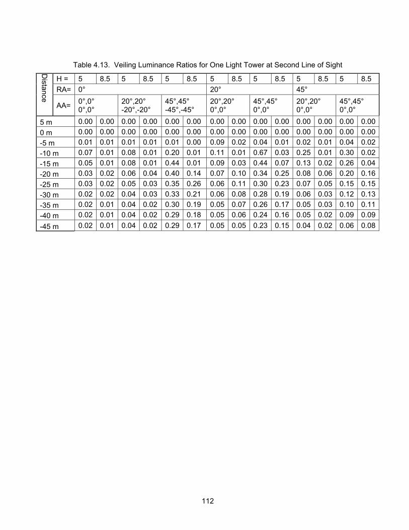
112
Table 4.13. Veiling Luminance Ratios for One Light Tower at Second Line of Sight
H = 5 8.5 5 8.5 5 8.5 5 8.5 5 8.5 5 8.5 5 8.5 RA= 0° 20° 45°
Distance
AA= 0°,0° 0°,0°
20°,20° -20°,-20°
45°,45° -45°,-45°
20°,20° 0°,0°
45°,45° 0°,0°
20°,20° 0°,0°
45°,45° 0°,0°
5 m 0.00 0.00 0.00 0.00 0.00 0.00 0.00 0.00 0.00 0.00 0.00 0.00 0.00 0.000 m 0.00 0.00 0.00 0.00 0.00 0.00 0.00 0.00 0.00 0.00 0.00 0.00 0.00 0.00-5 m 0.01 0.01 0.01 0.01 0.01 0.00 0.09 0.02 0.04 0.01 0.02 0.01 0.04 0.02-10 m 0.07 0.01 0.08 0.01 0.20 0.01 0.11 0.01 0.67 0.03 0.25 0.01 0.30 0.02-15 m 0.05 0.01 0.08 0.01 0.44 0.01 0.09 0.03 0.44 0.07 0.13 0.02 0.26 0.04-20 m 0.03 0.02 0.06 0.04 0.40 0.14 0.07 0.10 0.34 0.25 0.08 0.06 0.20 0.16-25 m 0.03 0.02 0.05 0.03 0.35 0.26 0.06 0.11 0.30 0.23 0.07 0.05 0.15 0.15-30 m 0.02 0.02 0.04 0.03 0.33 0.21 0.06 0.08 0.28 0.19 0.06 0.03 0.12 0.13-35 m 0.02 0.01 0.04 0.02 0.30 0.19 0.05 0.07 0.26 0.17 0.05 0.03 0.10 0.11-40 m 0.02 0.01 0.04 0.02 0.29 0.18 0.05 0.06 0.24 0.16 0.05 0.02 0.09 0.09-45 m 0.02 0.01 0.04 0.02 0.29 0.17 0.05 0.05 0.23 0.15 0.04 0.02 0.06 0.08

113
Table 4.14A. Average Horizontal Illuminance and Lighting Uniformity Ratios for One Light Tower
Test Arrangement #
Work Area Length in meters
Average Horizontal Illuminance in lux (Eavg)
Lighting Uniformity Ratio (U)
20 1310.82 119.82 30 936.93 439.87 11
40 728.88 1104.37 20 679.66 13.25 30 487.39 75.56 12 40 379.38 291.83 20 825.60 6.82 30 598.84 21.78 13 40 468.21 43.76 20 1010.66 71.07 30 723.30 159.67 14 40 562.85 678.13 20 978.63 36.65 30 701.79 115.62 15 40 546.76 166.70 20 944.92 154.40 30 675.94 734.71 16 40 525.92 674.26 20 695.84 63.26 30 498.38 124.59 17 40 387.94 484.92 20 749.64 16.81 30 537.10 95.06 18 40 418.17 224.82 20 620.76 7.76 30 450.20 18.92 19 40 351.85 47.16

114
Table 4.14B. Average Horizontal Illuminance and Lighting Uniformity Ratios for One Light Tower (Continued)
Test Arrangement #
Work Area Length in meters
Average Horizontal Illuminance in lux (Eavg)
Lighting Uniformity Ratio (U)
20 557.40 1.67 30 421.09 5.58 20
40 332.90 14.05 20 686.99 19.97 30 495.41 37.53 21 40 386.34 140.49 20 619.65 8.45 30 449.94 22.61 22 40 352.03 58.48 20 593.06 24.71 30 427.22 59.17 23 40 332.92 141.67 20 527.73 20.78
30 381.40 38.06 24
40 297.63 107.84
The main findings of the above tested lighting arrangements for one light tower include: (1) Veiling luminance ratio/glare steadily increases for drive by motorists as they approach
the light source and it reaches a peak between 10 m and 15 m before the light tower for the 5 m light height while the peak glare value for the 8.5 m height was observed between 20 m and 25 m before the light, as shown in Tables 4.12 and 4.13 and Figures 4.50 to 4.63.
(2) The rotation and aiming angles of the light tower luminaries have an impact on the veiling luminance ratios experienced at both lines of sight.
(3) For the second line of sight in all the tested heights, the veiling luminance ratios exceeded the 0.4 in two lighting arrangements as follows:
3.1) For the 5 m height and 0° and 45° rotation and aiming angles, the locations where the veiling luminance ratios exceeded 0.4 were at 15 m and 20 m before the light tower, as shown in Table 4.13;
3.2) For the 5 m height and 20° and 45° rotation and aiming angles, the locations where the veiling luminance ratios exceeded 0.4 were at 10 m and 15 m before the light tower, as shown in Table 4.13.
(4) For the first line of sight in all the tested heights, the 0.4 veiling luminance ratio was exceeded in two lighting arrangements as follows:
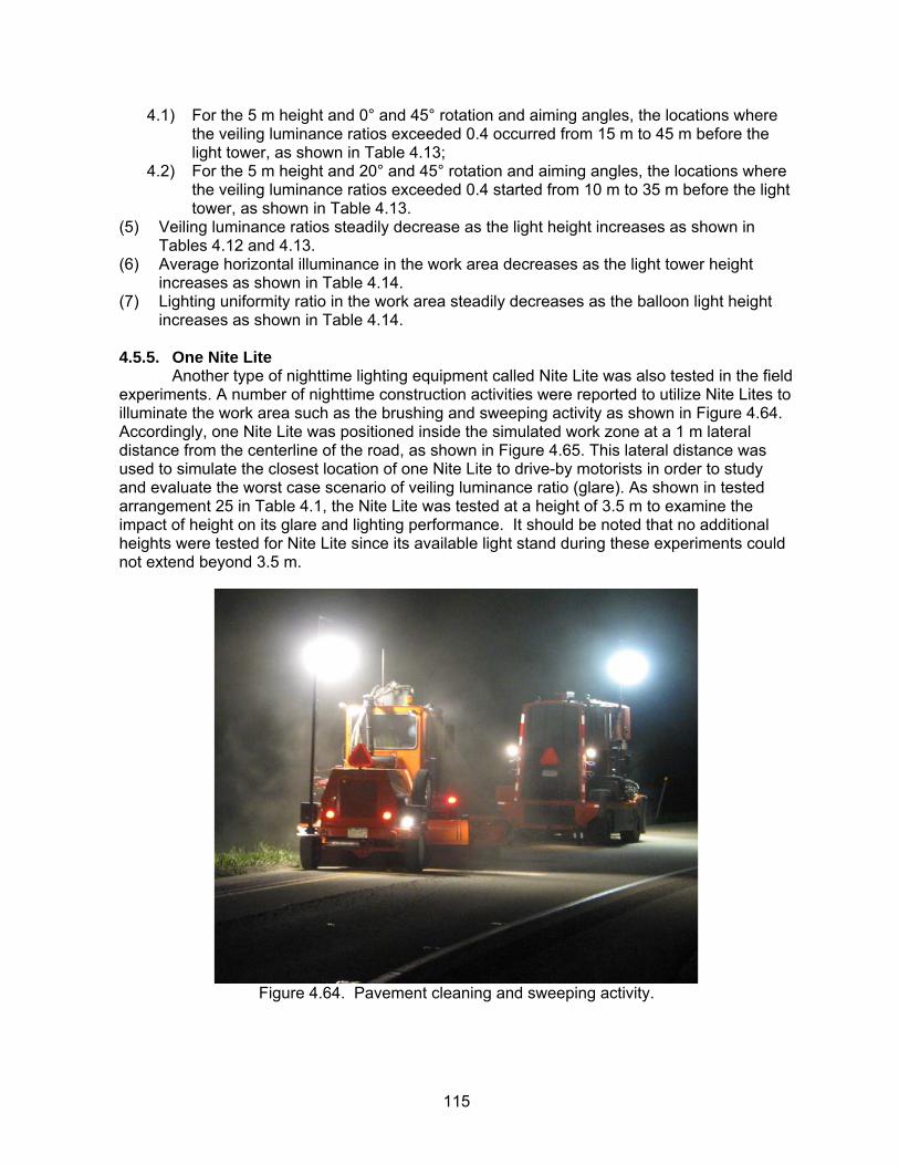
115
4.1) For the 5 m height and 0° and 45° rotation and aiming angles, the locations where the veiling luminance ratios exceeded 0.4 occurred from 15 m to 45 m before the light tower, as shown in Table 4.13;
4.2) For the 5 m height and 20° and 45° rotation and aiming angles, the locations where the veiling luminance ratios exceeded 0.4 started from 10 m to 35 m before the light tower, as shown in Table 4.13.
(5) Veiling luminance ratios steadily decrease as the light height increases as shown in Tables 4.12 and 4.13.
(6) Average horizontal illuminance in the work area decreases as the light tower height increases as shown in Table 4.14.
(7) Lighting uniformity ratio in the work area steadily decreases as the balloon light height increases as shown in Table 4.14.
4.5.5. One Nite Lite Another type of nighttime lighting equipment called Nite Lite was also tested in the field experiments. A number of nighttime construction activities were reported to utilize Nite Lites to illuminate the work area such as the brushing and sweeping activity as shown in Figure 4.64. Accordingly, one Nite Lite was positioned inside the simulated work zone at a 1 m lateral distance from the centerline of the road, as shown in Figure 4.65. This lateral distance was used to simulate the closest location of one Nite Lite to drive-by motorists in order to study and evaluate the worst case scenario of veiling luminance ratio (glare). As shown in tested arrangement 25 in Table 4.1, the Nite Lite was tested at a height of 3.5 m to examine the impact of height on its glare and lighting performance. It should be noted that no additional heights were tested for Nite Lite since its available light stand during these experiments could not extend beyond 3.5 m.
Figure 4.64. Pavement cleaning and sweeping activity.
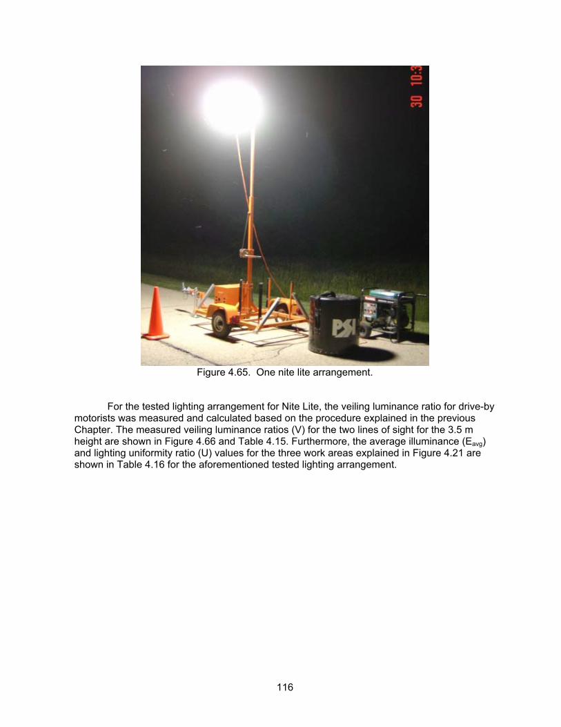
116
Figure 4.65. One nite lite arrangement.
For the tested lighting arrangement for Nite Lite, the veiling luminance ratio for drive-by motorists was measured and calculated based on the procedure explained in the previous Chapter. The measured veiling luminance ratios (V) for the two lines of sight for the 3.5 m height are shown in Figure 4.66 and Table 4.15. Furthermore, the average illuminance (Eavg) and lighting uniformity ratio (U) values for the three work areas explained in Figure 4.21 are shown in Table 4.16 for the aforementioned tested lighting arrangement.
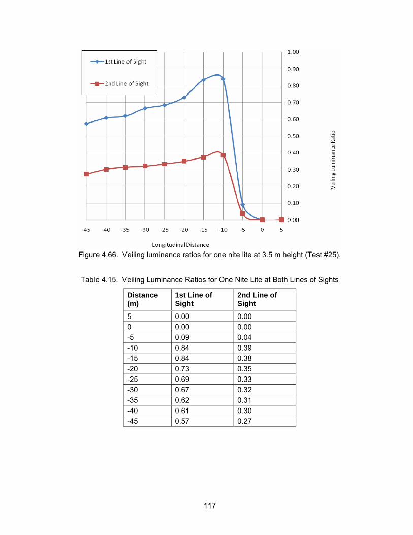
117
Figure 4.66. Veiling luminance ratios for one nite lite at 3.5 m height (Test #25).
Table 4.15. Veiling Luminance Ratios for One Nite Lite at Both Lines of Sights
Distance (m)
1st Line of Sight
2nd Line of Sight
5 0.00 0.00 0 0.00 0.00 -5 0.09 0.04 -10 0.84 0.39 -15 0.84 0.38 -20 0.73 0.35 -25 0.69 0.33 -30 0.67 0.32 -35 0.62 0.31 -40 0.61 0.30 -45 0.57 0.27
118
Table 4.16. Average Horizontal Illuminance and Lighting Uniformity Ratios for Nite Lite
Nite Lite Height in meters (H)
Work Area Length in meters
Average Horizontal Illuminance in lux (Eavg)
Lighting Uniformity Ratio (U)
20 84.59 11
30 61.13 25.47 Nite Lite
40 47.79 45.51
The main findings of the above tested lighting arrangement for the Nite Lite include: (1) Veiling luminance ratio steadily increases for drive-by motorists as they approach the
Nite Lite and reaches a peak at 10 m before the light source for the tested 3.5 m height, as shown in Table 4.15 and Figure 4.66.
(2) Veiling luminance ratios experienced at the first line of sight are consistently higher than those observed at the second line of sight, as shown in Figure 4.66.
(3) For the second line of sight in all the tested heights, the veiling luminance ratios in all locations were less than 0.4, as shown in Table 4.15.
(4) The veiling luminance ratio for the Nite Lite at the first line of sight exceeded 0.4 in a distance that extends from 10 m up to 45 m before the light source, as shown in Table 4.15.
119
CHAPTER 5 RECOMMENDATIONS TO CONTROL AND REDUCE GLARE 5. Based on the results of the conducted field experiments, the following two main sections of this Chapter present (1) a summary of the impact of the tested lighting parameters on the lighting performance in and around nighttime work zones; and (2) a number of practical recommendations that can be used to control and reduce glare caused by lighting arrangements in nighttime highway construction.
5.1. Impact of Tested Parameters on Lighting Performance This section summarizes the impact of the tested lighting parameters of (1) type of light; (2) height of light; (3) aiming and rotation angles of light towers, and (4) height of vehicle/observer on the veiling luminance ratio experienced by drive-by motorists as well as their impact on average horizontal illuminance and lighting uniformity ratio in the work area.
5.1.1. Type of Lighting The results of the conducted experiments illustrate that the type of lighting has an important impact on the veiling luminance ratio experienced by drive-by motorists. To evaluate the impact of the type of lighting, two sets of experiments were conducted to compare (1) one balloon light and one Nite Lite at a height of 3.5 m; and (2) one balloon light and one light tower at a height of 5 m. These experiments were divided into two sets because the available light stand for the Nite Lite during the field experiments could not extend beyond 3.5 m and the least practical height for the utilized light tower was 5m. In the first set of experiments to compare the balloon light and Nite Lite, the test results indicate that the balloon light generated 33% less average veiling luminance ratio (Vavg) than the Nite Lite at the first line of sight when both were tested at a height of 3.5 m. Similarly at the same tested height, the balloon light generated 23% less maximum veiling luminance ratio (Vmax) than the Nite Lite at the first line of sight, as shown in Figure 5.1 and Table 5.1. The test results also indicate that the balloon light and the Nite Lite at a height of 3.5 m generated very similar values of average horizontal illuminance (Eavg) and lighting uniformity ratio (U) with a difference less than 6%, as shown in Table 5.2.

120
Figure 5.1. Veiling luminance ratios caused by balloon light and nite lite at first line of sight.
Table 5.1. Veiling Luminance Ratios Caused by Balloon Light and Nite Lite at First Line of
Sight
Distance from Light Source (m) Nite Lite Balloon Light
5 0.00 0.00 0 0.00 0.00 -5 0.09 0.09 -10 0.84 0.64 -15 0.84 0.57 -20 0.73 0.51 -25 0.69 0.46 -30 0.67 0.44 -35 0.62 0.38 -40 0.61 0.35 -45 0.57 0.32 Average Veiling Luminance Ratio (Vavg)
0.51 0.34
% Reduction in Vavg Over Nite Lite 0% -33%
Maximum Veiling Luminance Ratio (Vmax)
0.84 0.64
% Reduction in Vmax Over Nite Lite 0% -23%
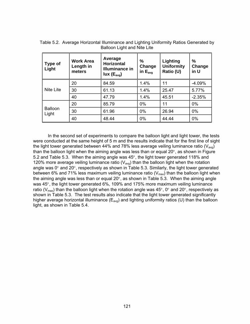
121
Table 5.2. Average Horizontal Illuminance and Lighting Uniformity Ratios Generated by Balloon Light and Nite Lite
Type of Light
Work Area Length in meters
Average Horizontal Illuminance in lux (Eavg)
% Change in Eavg
Lighting Uniformity Ratio (U)
% Change in U
20 84.59 1.4% 11 -4.09% 30 61.13 1.4% 25.47 5.77% Nite Lite 40 47.79 1.4% 45.51 -2.35% 20 85.79 0% 11 0% 30 61.96 0% 26.94 0% Balloon
Light 40 48.44 0% 44.44 0%
In the second set of experiments to compare the balloon light and light tower, the tests were conducted at the same height of 5 m and the results indicate that for the first line of sight the light tower generated between 44% and 78% less average veiling luminance ratio (Vavg) than the balloon light when the aiming angle was less than or equal 20°, as shown in Figure 5.2 and Table 5.3. When the aiming angle was 45°, the light tower generated 118% and 120% more average veiling luminance ratio (Vavg) than the balloon light when the rotation angle was 0° and 20°, respectively as shown in Table 5.3. Similarly, the light tower generated between 6% and 71% less maximum veiling luminance ratio (Vmax) than the balloon light when the aiming angle was less than or equal 20°, as shown in Table 5.3. When the aiming angle was 45°, the light tower generated 6%, 109% and 175% more maximum veiling luminance ratio (Vmax) than the balloon light when the rotation angle was 45°, 0° and 20°, respectively as shown in Table 5.3. The test results also indicate that the light tower generated significantly higher average horizontal illuminance (Eavg) and lighting uniformity ratios (U) than the balloon light, as shown in Table 5.4.
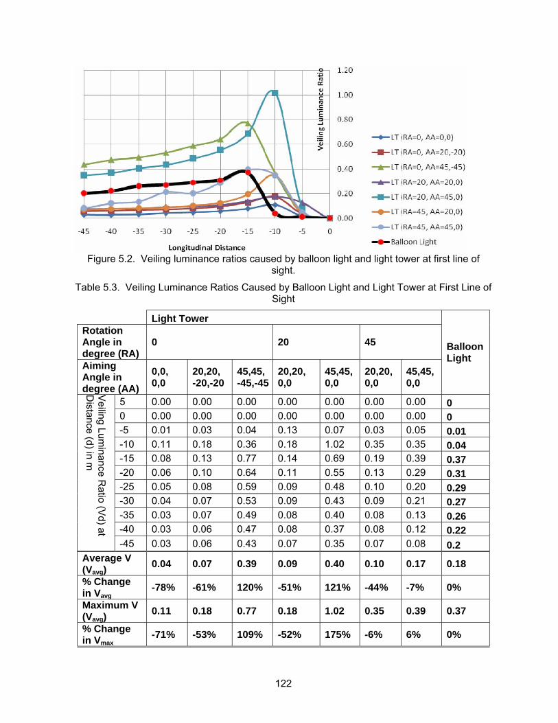
122
Figure 5.2. Veiling luminance ratios caused by balloon light and light tower at first line of
sight.
Table 5.3. Veiling Luminance Ratios Caused by Balloon Light and Light Tower at First Line of Sight
Light Tower Rotation Angle in degree (RA)
0 20 45
Aiming Angle in degree (AA)
0,0, 0,0
20,20, -20,-20
45,45, -45,-45
20,20, 0,0
45,45, 0,0
20,20, 0,0
45,45, 0,0
Balloon Light
5 0.00 0.00 0.00 0.00 0.00 0.00 0.00 0 0 0.00 0.00 0.00 0.00 0.00 0.00 0.00 0 -5 0.01 0.03 0.04 0.13 0.07 0.03 0.05 0.01 -10 0.11 0.18 0.36 0.18 1.02 0.35 0.35 0.04 -15 0.08 0.13 0.77 0.14 0.69 0.19 0.39 0.37 -20 0.06 0.10 0.64 0.11 0.55 0.13 0.29 0.31 -25 0.05 0.08 0.59 0.09 0.48 0.10 0.20 0.29 -30 0.04 0.07 0.53 0.09 0.43 0.09 0.21 0.27 -35 0.03 0.07 0.49 0.08 0.40 0.08 0.13 0.26 -40 0.03 0.06 0.47 0.08 0.37 0.08 0.12 0.22
Veiling Lum
inance Ratio (V
d) at D
istance (d) in m
-45 0.03 0.06 0.43 0.07 0.35 0.07 0.08 0.2 Average V (Vavg)
0.04 0.07 0.39 0.09 0.40 0.10 0.17 0.18
% Change in Vavg
-78% -61% 120% -51% 121% -44% -7% 0%
Maximum V (Vavg)
0.11 0.18 0.77 0.18 1.02 0.35 0.39 0.37
% Change in Vmax
-71% -53% 109% -52% 175% -6% 6% 0%
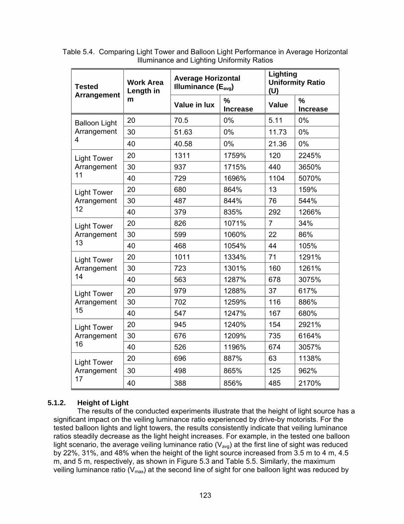
123
Table 5.4. Comparing Light Tower and Balloon Light Performance in Average Horizontal Illuminance and Lighting Uniformity Ratios
Average Horizontal Illuminance (Eavg)
Lighting Uniformity Ratio (U) Tested
Arrangement Work Area Length in m
Value in lux % Increase Value %
Increase 20 70.5 0% 5.11 0% 30 51.63 0% 11.73 0%
Balloon Light Arrangement 4 40 40.58 0% 21.36 0%
20 1311 1759% 120 2245% 30 937 1715% 440 3650%
Light Tower Arrangement 11 40 729 1696% 1104 5070%
20 680 864% 13 159% 30 487 844% 76 544%
Light Tower Arrangement 12 40 379 835% 292 1266%
20 826 1071% 7 34% 30 599 1060% 22 86%
Light Tower Arrangement 13 40 468 1054% 44 105%
20 1011 1334% 71 1291% 30 723 1301% 160 1261%
Light Tower Arrangement 14 40 563 1287% 678 3075%
20 979 1288% 37 617% 30 702 1259% 116 886%
Light Tower Arrangement 15 40 547 1247% 167 680%
20 945 1240% 154 2921% 30 676 1209% 735 6164%
Light Tower Arrangement 16 40 526 1196% 674 3057%
20 696 887% 63 1138%
30 498 865% 125 962% Light Tower Arrangement 17 40 388 856% 485 2170%
5.1.2. Height of Light
The results of the conducted experiments illustrate that the height of light source has a significant impact on the veiling luminance ratio experienced by drive-by motorists. For the tested balloon lights and light towers, the results consistently indicate that veiling luminance ratios steadily decrease as the light height increases. For example, in the tested one balloon light scenario, the average veiling luminance ratio (Vavg) at the first line of sight was reduced by 22%, 31%, and 48% when the height of the light source increased from 3.5 m to 4 m, 4.5 m, and 5 m, respectively, as shown in Figure 5.3 and Table 5.5. Similarly, the maximum veiling luminance ratio (Vmax) at the second line of sight for one balloon light was reduced by
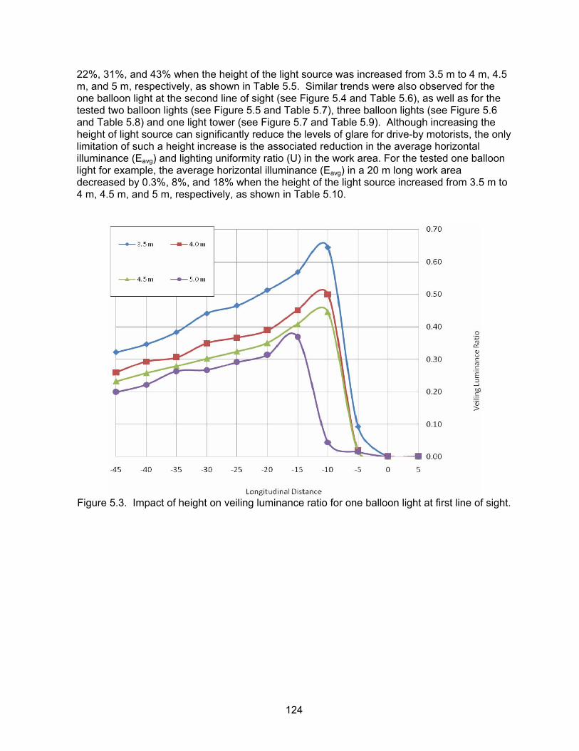
124
22%, 31%, and 43% when the height of the light source was increased from 3.5 m to 4 m, 4.5 m, and 5 m, respectively, as shown in Table 5.5. Similar trends were also observed for the one balloon light at the second line of sight (see Figure 5.4 and Table 5.6), as well as for the tested two balloon lights (see Figure 5.5 and Table 5.7), three balloon lights (see Figure 5.6 and Table 5.8) and one light tower (see Figure 5.7 and Table 5.9). Although increasing the height of light source can significantly reduce the levels of glare for drive-by motorists, the only limitation of such a height increase is the associated reduction in the average horizontal illuminance (Eavg) and lighting uniformity ratio (U) in the work area. For the tested one balloon light for example, the average horizontal illuminance (Eavg) in a 20 m long work area decreased by 0.3%, 8%, and 18% when the height of the light source increased from 3.5 m to 4 m, 4.5 m, and 5 m, respectively, as shown in Table 5.10.
Figure 5.3. Impact of height on veiling luminance ratio for one balloon light at first line of sight.
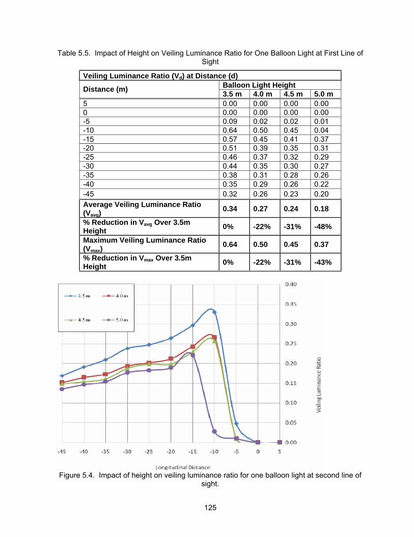
125
Table 5.5. Impact of Height on Veiling Luminance Ratio for One Balloon Light at First Line of Sight
Veiling Luminance Ratio (Vd) at Distance (d) Balloon Light Height Distance (m) 3.5 m 4.0 m 4.5 m 5.0 m
5 0.00 0.00 0.00 0.00 0 0.00 0.00 0.00 0.00 -5 0.09 0.02 0.02 0.01 -10 0.64 0.50 0.45 0.04 -15 0.57 0.45 0.41 0.37 -20 0.51 0.39 0.35 0.31 -25 0.46 0.37 0.32 0.29 -30 0.44 0.35 0.30 0.27 -35 0.38 0.31 0.28 0.26 -40 0.35 0.29 0.26 0.22 -45 0.32 0.26 0.23 0.20 Average Veiling Luminance Ratio (Vavg)
0.34 0.27 0.24 0.18
% Reduction in Vavg Over 3.5m Height 0% -22% -31% -48%
Maximum Veiling Luminance Ratio (Vmax)
0.64 0.50 0.45 0.37
% Reduction in Vmax Over 3.5m Height 0% -22% -31% -43%
Figure 5.4. Impact of height on veiling luminance ratio for one balloon light at second line of
sight.
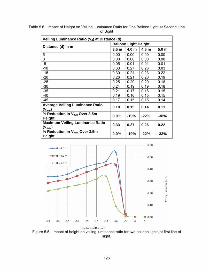
126
Table 5.6. Impact of Height on Veiling Luminance Ratio for One Balloon Light at Second Line of Sight
Veiling Luminance Ratio (Vd) at Distance (d) Balloon Light Height Distance (d) in m 3.5 m 4.0 m 4.5 m 5.0 m
5 0.00 0.00 0.00 0.00 0 0.00 0.00 0.00 0.00 -5 0.05 0.01 0.01 0.01 -10 0.33 0.27 0.26 0.03 -15 0.30 0.24 0.23 0.22 -20 0.26 0.21 0.20 0.19 -25 0.25 0.20 0.20 0.18 -30 0.24 0.19 0.19 0.18 -35 0.21 0.17 0.16 0.15 -40 0.19 0.16 0.15 0.15 -45 0.17 0.15 0.15 0.14 Average Veiling Luminance Ratio (Vavg)
0.18 0.15 0.14 0.11
% Reduction in Vavg Over 3.5m Height 0.0% -19% -22% -38%
Maximum Veiling Luminance Ratio (Vmax)
0.33 0.27 0.26 0.22
% Reduction in Vmax Over 3.5m Height 0.0% -19% -22% -33%
Figure 5.5. Impact of height on veiling luminance ratio for two balloon lights at first line of
sight.

127
Table 5.7. Impact of Height on Veiling Luminance Ratio for Two Balloon Lights at First Line of
Sight
Veiling Luminance Ratio (Vd) at Distance (d) Balloon Light Height
Distance (m) 4.0 m 4.5 m 5.0 m
5 0.00 0.00 0.00 0 0.00 0.00 0.00 -5 0.01 0.03 0.01 -10 0.54 0.44 0.09 -15 0.47 0.43 0.34 -20 0.44 0.40 0.32 -25 0.42 0.37 0.29 -30 0.39 0.34 0.27 -35 0.36 0.32 0.25 -40 0.34 0.30 0.23 -45 0.34 0.29 0.22 Average Veiling Luminance Ratio (Vavg) 0.30 0.27 0.18 % Reduction in Vavg Over 5.0m Height 0.0% -12% -39% Maximum Veiling Luminance Ratio (Vmax) 0.54 0.44 0.34 % Reduction in Vmax Over 5.0m Height 0.0% -19% -37%
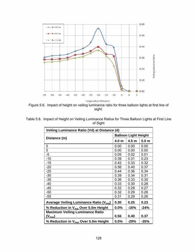
128
Figure 5.6. Impact of height on veiling luminance ratio for three balloon lights at first line of
sight.
Table 5.8. Impact of Height on Veiling Luminance Ratios for Three Balloon Lights at First Line
of Sight
Veiling Luminance Ratio (Vd) at Distance (d) Balloon Light Height
Distance (m) 4.0 m 4.5 m 5.0 m
5 0.00 0.00 0.00 0 0.00 0.00 0.00 -5 0.05 0.02 0.01 -10 0.39 0.31 0.23 -15 0.42 0.33 0.32 -20 0.56 0.40 0.37 -25 0.44 0.36 0.34 -30 0.39 0.34 0.31 -35 0.36 0.33 0.30 -40 0.33 0.30 0.28 -45 0.32 0.29 0.27 -50 0.32 0.29 0.26 -55 0.31 0.29 0.26
Average Veiling Luminance Ratio (Vavg) 0.30 0.25 0.23 % Reduction in Vavg Over 5.0m Height 0.0% -16% -24% Maximum Veiling Luminance Ratio (Vmax) 0.56 0.40 0.37 % Reduction in Vmax Over 5.0m Height 0.0% -29% -35%

129
Figure 5.7. Impact of height on veiling luminance ratio for one light tower at first line of sight
when rotation angle is 0° and aiming angles are 45°,45°,-45°,-45°.
Table 5.9. Impact of Height on Veiling Luminance Ratios for One Light Tower at First Line of Sight when Rotation Angle is 0° and Aiming Angles are 45°,45°,-45°,-45°
Height of Light Tower 5.0 m 8.5 m Rotation Angle 0°
Aiming Angle of Luminaries 45°,45°, -45°,-45°
5 0.00 0.00 0 0.00 0.00 -5 0.04 0.01 -10 0.36 0.02 -15 0.77 0.05 -20 0.64 0.19 -25 0.59 0.35 -30 0.53 0.27 -35 0.49 0.24 -40 0.47 0.22
Vei
ling
Lum
inan
ce R
atio
(Vd)
at
Dis
tanc
e (d
) in
m
-45 0.43 0.20 Average Veiling Luminance Ratio (Vavg)
0.39 0.14
% Reduction in Vavg Over 5.0m Height 0% -64% Maximum Veiling Luminance Ratio (Vmax)
0.77 0.35
% Reduction in Vmax Over 5.0m Height 0% -55%
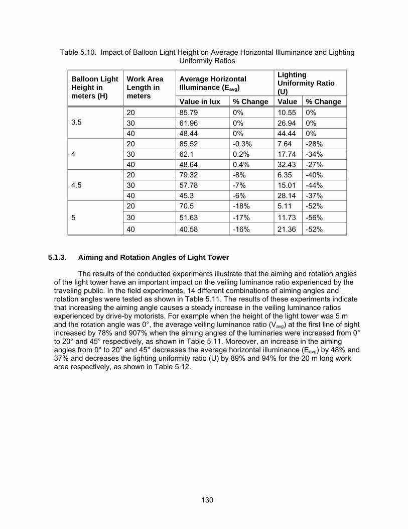
130
Table 5.10. Impact of Balloon Light Height on Average Horizontal Illuminance and Lighting Uniformity Ratios
Average Horizontal Illuminance (Eavg)
Lighting Uniformity Ratio (U)
Balloon Light Height in meters (H)
Work Area Length in meters
Value in lux % Change Value % Change 20 85.79 0% 10.55 0% 30 61.96 0% 26.94 0% 3.5 40 48.44 0% 44.44 0% 20 85.52 -0.3% 7.64 -28% 30 62.1 0.2% 17.74 -34% 4 40 48.64 0.4% 32.43 -27% 20 79.32 -8% 6.35 -40% 30 57.78 -7% 15.01 -44% 4.5 40 45.3 -6% 28.14 -37% 20 70.5 -18% 5.11 -52% 30 51.63 -17% 11.73 -56% 5 40 40.58 -16% 21.36 -52%
5.1.3. Aiming and Rotation Angles of Light Tower
The results of the conducted experiments illustrate that the aiming and rotation angles of the light tower have an important impact on the veiling luminance ratio experienced by the traveling public. In the field experiments, 14 different combinations of aiming angles and rotation angles were tested as shown in Table 5.11. The results of these experiments indicate that increasing the aiming angle causes a steady increase in the veiling luminance ratios experienced by drive-by motorists. For example when the height of the light tower was 5 m and the rotation angle was 0°, the average veiling luminance ratio (Vavg) at the first line of sight increased by 78% and 907% when the aiming angles of the luminaries were increased from 0° to 20° and 45° respectively, as shown in Table 5.11. Moreover, an increase in the aiming angles from 0° to 20° and 45° decreases the average horizontal illuminance (Eavg) by 48% and 37% and decreases the lighting uniformity ratio (U) by 89% and 94% for the 20 m long work area respectively, as shown in Table 5.12.
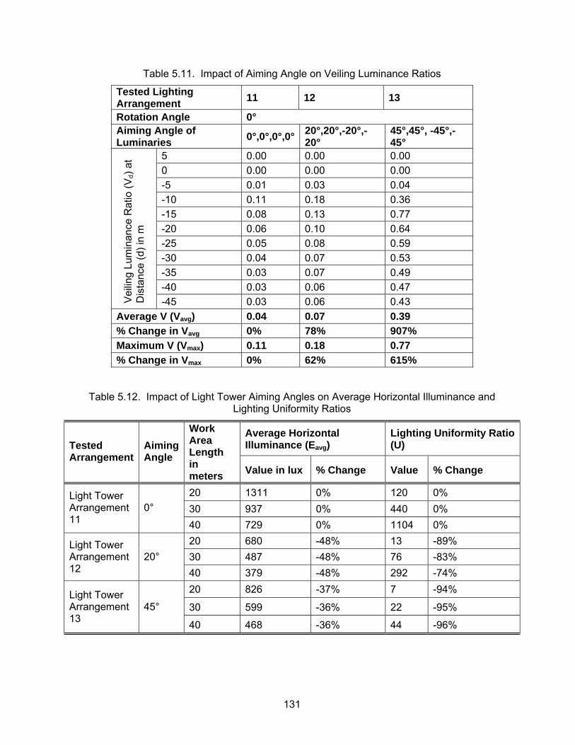
131
Table 5.11. Impact of Aiming Angle on Veiling Luminance Ratios
Tested Lighting Arrangement 11 12 13
Rotation Angle 0° Aiming Angle of Luminaries 0°,0°,0°,0° 20°,20°,-20°,-
20° 45°,45°, -45°,-45°
5 0.00 0.00 0.00 0 0.00 0.00 0.00 -5 0.01 0.03 0.04 -10 0.11 0.18 0.36 -15 0.08 0.13 0.77 -20 0.06 0.10 0.64 -25 0.05 0.08 0.59 -30 0.04 0.07 0.53 -35 0.03 0.07 0.49 -40 0.03 0.06 0.47
Vei
ling
Lum
inan
ce R
atio
(Vd)
at
Dis
tanc
e (d
) in
m
-45 0.03 0.06 0.43 Average V (Vavg) 0.04 0.07 0.39 % Change in Vavg 0% 78% 907% Maximum V (Vmax) 0.11 0.18 0.77 % Change in Vmax 0% 62% 615%
Table 5.12. Impact of Light Tower Aiming Angles on Average Horizontal Illuminance and
Lighting Uniformity Ratios
Average Horizontal Illuminance (Eavg)
Lighting Uniformity Ratio (U) Tested
Arrangement Aiming Angle
Work Area Length in meters Value in lux % Change Value % Change
20 1311 0% 120 0% 30 937 0% 440 0%
Light Tower Arrangement 11
0°
40 729 0% 1104 0% 20 680 -48% 13 -89% 30 487 -48% 76 -83%
Light Tower Arrangement 12
20° 40 379 -48% 292 -74% 20 826 -37% 7 -94%
30 599 -36% 22 -95% Light Tower Arrangement 13
45°
40 468 -36% 44 -96%
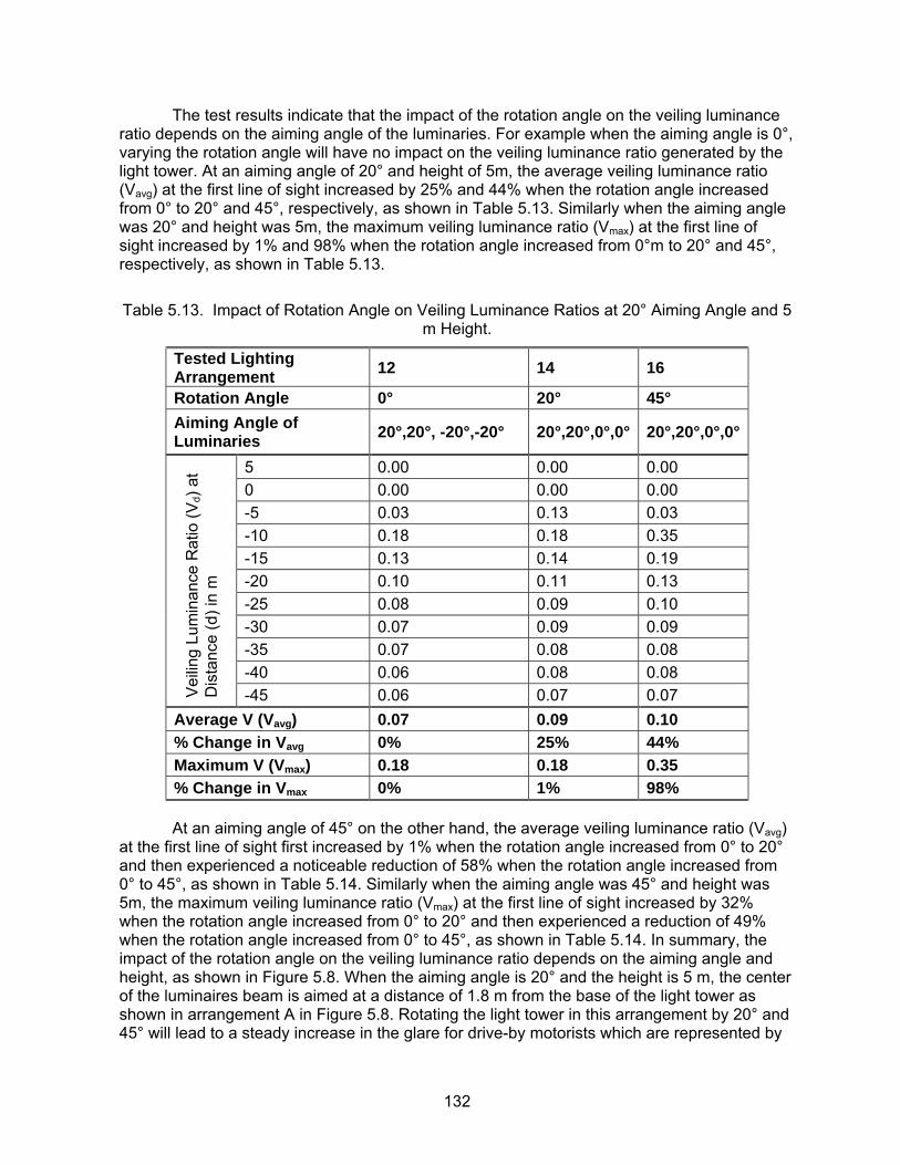
132
The test results indicate that the impact of the rotation angle on the veiling luminance ratio depends on the aiming angle of the luminaries. For example when the aiming angle is 0°, varying the rotation angle will have no impact on the veiling luminance ratio generated by the light tower. At an aiming angle of 20° and height of 5m, the average veiling luminance ratio (Vavg) at the first line of sight increased by 25% and 44% when the rotation angle increased from 0° to 20° and 45°, respectively, as shown in Table 5.13. Similarly when the aiming angle was 20° and height was 5m, the maximum veiling luminance ratio (Vmax) at the first line of sight increased by 1% and 98% when the rotation angle increased from 0°m to 20° and 45°, respectively, as shown in Table 5.13.
Table 5.13. Impact of Rotation Angle on Veiling Luminance Ratios at 20° Aiming Angle and 5 m Height.
Tested Lighting Arrangement 12 14 16
Rotation Angle 0° 20° 45° Aiming Angle of Luminaries 20°,20°, -20°,-20° 20°,20°,0°,0° 20°,20°,0°,0°
5 0.00 0.00 0.00 0 0.00 0.00 0.00 -5 0.03 0.13 0.03 -10 0.18 0.18 0.35 -15 0.13 0.14 0.19 -20 0.10 0.11 0.13 -25 0.08 0.09 0.10 -30 0.07 0.09 0.09 -35 0.07 0.08 0.08 -40 0.06 0.08 0.08
Vei
ling
Lum
inan
ce R
atio
(Vd)
at
Dis
tanc
e (d
) in
m
-45 0.06 0.07 0.07 Average V (Vavg) 0.07 0.09 0.10 % Change in Vavg 0% 25% 44% Maximum V (Vmax) 0.18 0.18 0.35 % Change in Vmax 0% 1% 98%
At an aiming angle of 45° on the other hand, the average veiling luminance ratio (Vavg) at the first line of sight first increased by 1% when the rotation angle increased from 0° to 20° and then experienced a noticeable reduction of 58% when the rotation angle increased from 0° to 45°, as shown in Table 5.14. Similarly when the aiming angle was 45° and height was 5m, the maximum veiling luminance ratio (Vmax) at the first line of sight increased by 32% when the rotation angle increased from 0° to 20° and then experienced a reduction of 49% when the rotation angle increased from 0° to 45°, as shown in Table 5.14. In summary, the impact of the rotation angle on the veiling luminance ratio depends on the aiming angle and height, as shown in Figure 5.8. When the aiming angle is 20° and the height is 5 m, the center of the luminaires beam is aimed at a distance of 1.8 m from the base of the light tower as shown in arrangement A in Figure 5.8. Rotating the light tower in this arrangement by 20° and 45° will lead to a steady increase in the glare for drive-by motorists which are represented by
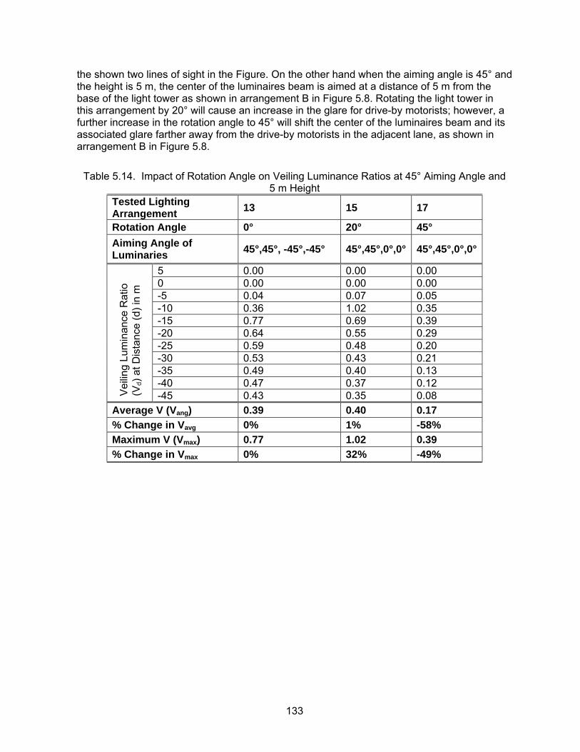
133
the shown two lines of sight in the Figure. On the other hand when the aiming angle is 45° and the height is 5 m, the center of the luminaires beam is aimed at a distance of 5 m from the base of the light tower as shown in arrangement B in Figure 5.8. Rotating the light tower in this arrangement by 20° will cause an increase in the glare for drive-by motorists; however, a further increase in the rotation angle to 45° will shift the center of the luminaires beam and its associated glare farther away from the drive-by motorists in the adjacent lane, as shown in arrangement B in Figure 5.8.
Table 5.14. Impact of Rotation Angle on Veiling Luminance Ratios at 45° Aiming Angle and 5 m Height
Tested Lighting Arrangement 13 15 17
Rotation Angle 0° 20° 45° Aiming Angle of Luminaries 45°,45°, -45°,-45° 45°,45°,0°,0° 45°,45°,0°,0°
5 0.00 0.00 0.00 0 0.00 0.00 0.00 -5 0.04 0.07 0.05 -10 0.36 1.02 0.35 -15 0.77 0.69 0.39 -20 0.64 0.55 0.29 -25 0.59 0.48 0.20 -30 0.53 0.43 0.21 -35 0.49 0.40 0.13 -40 0.47 0.37 0.12
Vei
ling
Lum
inan
ce R
atio
(V
d) a
t Dis
tanc
e (d
) in
m
-45 0.43 0.35 0.08 Average V (Vang) 0.39 0.40 0.17 % Change in Vavg 0% 1% -58% Maximum V (Vmax) 0.77 1.02 0.39 % Change in Vmax 0% 32% -49%
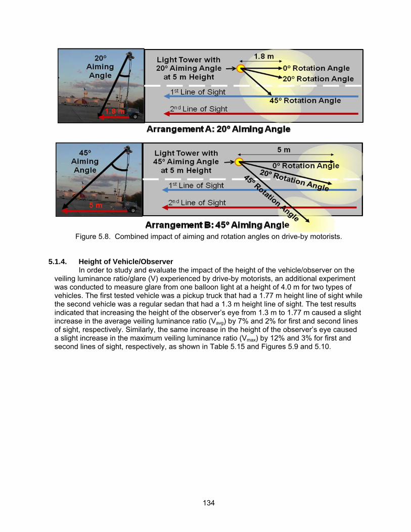
134
Figure 5.8. Combined impact of aiming and rotation angles on drive-by motorists.
5.1.4. Height of Vehicle/Observer In order to study and evaluate the impact of the height of the vehicle/observer on the veiling luminance ratio/glare (V) experienced by drive-by motorists, an additional experiment was conducted to measure glare from one balloon light at a height of 4.0 m for two types of vehicles. The first tested vehicle was a pickup truck that had a 1.77 m height line of sight while the second vehicle was a regular sedan that had a 1.3 m height line of sight. The test results indicated that increasing the height of the observer’s eye from 1.3 m to 1.77 m caused a slight increase in the average veiling luminance ratio (Vavg) by 7% and 2% for first and second lines of sight, respectively. Similarly, the same increase in the height of the observer’s eye caused a slight increase in the maximum veiling luminance ratio (Vmax) by 12% and 3% for first and second lines of sight, respectively, as shown in Table 5.15 and Figures 5.9 and 5.10.
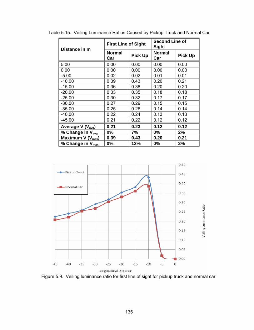
135
Table 5.15. Veiling Luminance Ratios Caused by Pickup Truck and Normal Car
First Line of Sight Second Line of Sight Distance in m
Normal Car Pick Up Normal
Car Pick Up
5.00 0.00 0.00 0.00 0.00 0.00 0.00 0.00 0.00 0.00 -5.00 0.02 0.02 0.01 0.01 -10.00 0.39 0.43 0.20 0.21 -15.00 0.36 0.38 0.20 0.20 -20.00 0.33 0.35 0.18 0.18 -25.00 0.30 0.32 0.17 0.17 -30.00 0.27 0.29 0.15 0.15 -35.00 0.25 0.26 0.14 0.14 -40.00 0.22 0.24 0.13 0.13 -45.00 0.21 0.22 0.12 0.12 Average V (Vavg) 0.21 0.23 0.12 0.12 % Change in Vavg 0% 7% 0% 2% Maximum V (Vmax) 0.39 0.43 0.20 0.21 % Change in Vmax 0% 12% 0% 3%
Figure 5.9. Veiling luminance ratio for first line of sight for pickup truck and normal car.
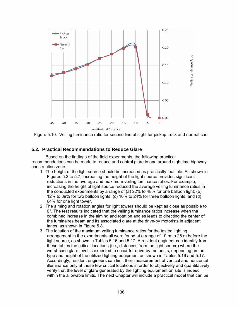
136
Figure 5.10. Veiling luminance ratio for second line of sight for pickup truck and normal car.
5.2. Practical Recommendations to Reduce Glare Based on the findings of the field experiments, the following practical recommendations can be made to reduce and control glare in and around nighttime highway construction zone:
1. The height of the light source should be increased as practically feasible. As shown in Figures 5.3 to 5.7, increasing the height of the light source provides significant reductions in the average and maximum veiling luminance ratios. For example, increasing the height of light source reduced the average veiling luminance ratios in the conducted experiments by a range of (a) 22% to 48% for one balloon light; (b) 12% to 39% for two balloon lights; (c) 16% to 24% for three balloon lights; and (d) 64% for one light tower.
2. The aiming and rotation angles for light towers should be kept as close as possible to 0°. The test results indicated that the veiling luminance ratios increase when the combined increase in the aiming and rotation angles leads to directing the center of the luminaires beam and its associated glare at the drive-by motorists in adjacent lanes, as shown in Figure 5.8.
3. The location of the maximum veiling luminance ratios for the tested lighting arrangement in the experiments all were found at a range of 10 m to 25 m before the light source, as shown in Tables 5.16 and 5.17. A resident engineer can identify from these tables the critical locations (i.e., distances from the light source) where the worst-case glare level is expected to occur for drive-by motorists, depending on the type and height of the utilized lighting equipment as shown in Tables 5.16 and 5.17. Accordingly, resident engineers can limit their measurement of vertical and horizontal illuminance only at these few critical locations in order to objectively and quantitatively verify that the level of glare generated by the lighting equipment on site is indeed within the allowable limits. The next Chapter will include a practical model that can be
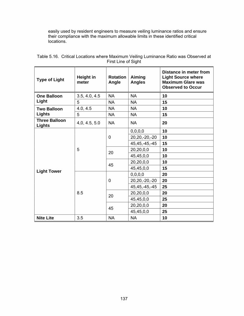
137
easily used by resident engineers to measure veiling luminance ratios and ensure their compliance with the maximum allowable limits in these identified critical locations.
Table 5.16. Critical Locations where Maximum Veiling Luminance Ratio was Observed at First Line of Sight
Type of Light Height in meter
Rotation Angle
Aiming Angles
Distance in meter from Light Source where Maximum Glare was Observed to Occur
3.5, 4.0, 4.5 NA NA 10 One Balloon Light 5 NA NA 15
4.0, 4.5 NA NA 10 Two Balloon Lights 5 NA NA 15 Three Balloon Lights 4,0, 4.5, 5.0 NA NA 20
0,0,0,0 10 20,20,-20,-20 10 0 45,45,-45,-45 15 20,20,0,0 10
20 45,45,0,0 10 20,20,0,0 10
5
45 45,45,0,0 15 0,0,0,0 20 20,20,-20,-20 20 0 45,45,-45,-45 25 20,20,0,0 20
20 45,45,0,0 25 20,20,0,0 20
Light Tower
8.5
45 45,45,0,0 25
Nite Lite 3.5 NA NA 10
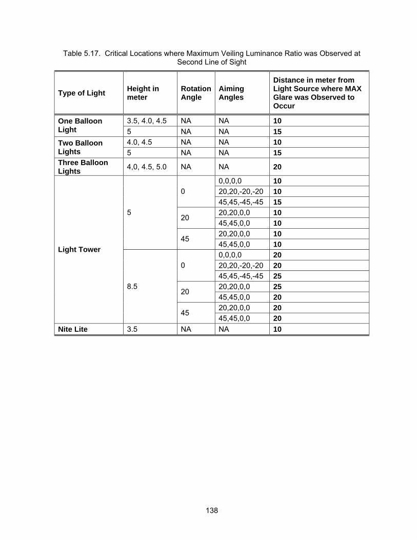
138
Table 5.17. Critical Locations where Maximum Veiling Luminance Ratio was Observed at Second Line of Sight
Type of Light Height in meter
Rotation Angle
Aiming Angles
Distance in meter from Light Source where MAX Glare was Observed to Occur
3.5, 4.0, 4.5 NA NA 10 One Balloon Light 5 NA NA 15
4.0, 4.5 NA NA 10 Two Balloon Lights 5 NA NA 15 Three Balloon Lights 4,0, 4.5, 5.0 NA NA 20
0,0,0,0 10 20,20,-20,-20 10 0 45,45,-45,-45 15 20,20,0,0 10
20 45,45,0,0 10 20,20,0,0 10
5
45 45,45,0,0 10 0,0,0,0 20 20,20,-20,-20 20 0 45,45,-45,-45 25 20,20,0,0 25
20 45,45,0,0 20 20,20,0,0 20
Light Tower
8.5
45 45,45,0,0 20
Nite Lite 3.5 NA NA 10
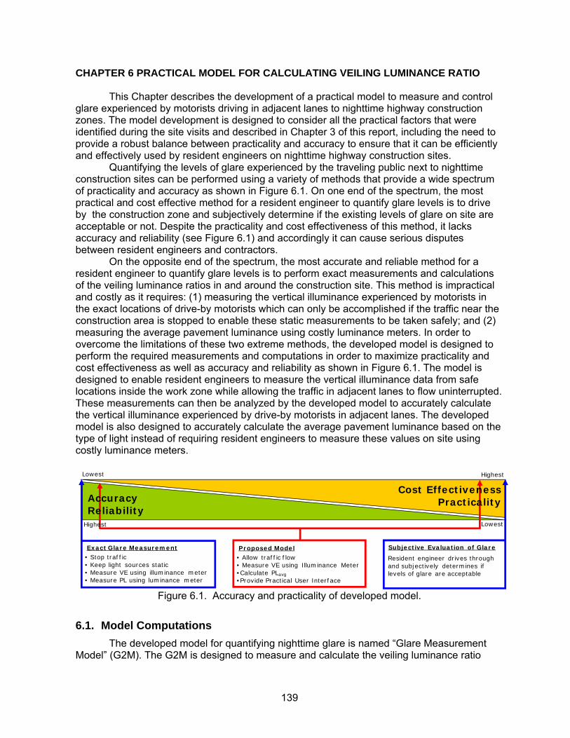
139
CHAPTER 6 PRACTICAL MODEL FOR CALCULATING VEILING LUMINANCE RATIO 6. 2 This Chapter describes the development of a practical model to measure and control glare experienced by motorists driving in adjacent lanes to nighttime highway construction zones. The model development is designed to consider all the practical factors that were identified during the site visits and described in Chapter 3 of this report, including the need to provide a robust balance between practicality and accuracy to ensure that it can be efficiently and effectively used by resident engineers on nighttime highway construction sites. Quantifying the levels of glare experienced by the traveling public next to nighttime construction sites can be performed using a variety of methods that provide a wide spectrum of practicality and accuracy as shown in Figure 6.1. On one end of the spectrum, the most practical and cost effective method for a resident engineer to quantify glare levels is to drive by the construction zone and subjectively determine if the existing levels of glare on site are acceptable or not. Despite the practicality and cost effectiveness of this method, it lacks accuracy and reliability (see Figure 6.1) and accordingly it can cause serious disputes between resident engineers and contractors. On the opposite end of the spectrum, the most accurate and reliable method for a resident engineer to quantify glare levels is to perform exact measurements and calculations of the veiling luminance ratios in and around the construction site. This method is impractical and costly as it requires: (1) measuring the vertical illuminance experienced by motorists in the exact locations of drive-by motorists which can only be accomplished if the traffic near the construction area is stopped to enable these static measurements to be taken safely; and (2) measuring the average pavement luminance using costly luminance meters. In order to overcome the limitations of these two extreme methods, the developed model is designed to perform the required measurements and computations in order to maximize practicality and cost effectiveness as well as accuracy and reliability as shown in Figure 6.1. The model is designed to enable resident engineers to measure the vertical illuminance data from safe locations inside the work zone while allowing the traffic in adjacent lanes to flow uninterrupted. These measurements can then be analyzed by the developed model to accurately calculate the vertical illuminance experienced by drive-by motorists in adjacent lanes. The developed model is also designed to accurately calculate the average pavement luminance based on the type of light instead of requiring resident engineers to measure these values on site using costly luminance meters.
Lowest
HighestLowest
• Stop traff ic• Keep light sources static• Measure VE using illuminance meter• Measure PL using luminance meter
Resident engineer drives through and subjectively determines if levels of glare are acceptable
Exact Glare Measurement Subjective Evaluation of Glare
AccuracyReliability
Cost EffectivenessPracticality
Highest
• Allow traff ic f low• Measure VE using Illuminance Meter•Calculate PLavg
•Provide Practical User Interface
Proposed Model
Figure 6.1. Accuracy and practicality of developed model.
6.1. Model Computations The developed model for quantifying nighttime glare is named “Glare Measurement Model” (G2M). The G2M is designed to measure and calculate the veiling luminance ratio
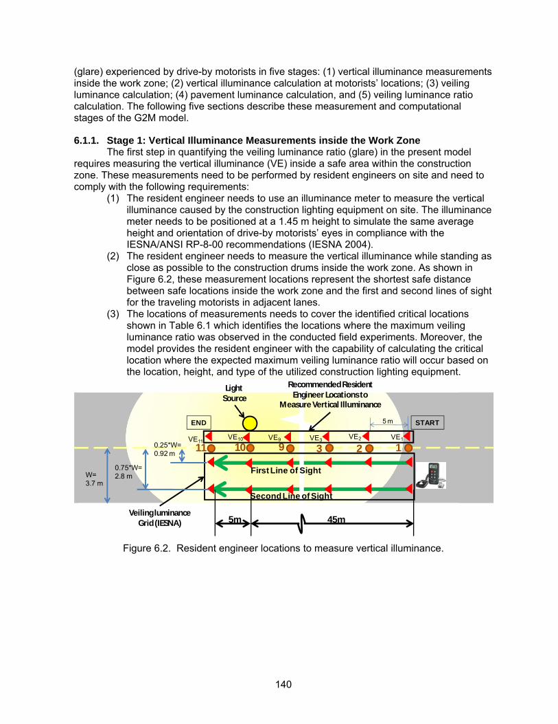
140
(glare) experienced by drive-by motorists in five stages: (1) vertical illuminance measurements inside the work zone; (2) vertical illuminance calculation at motorists’ locations; (3) veiling luminance calculation; (4) pavement luminance calculation, and (5) veiling luminance ratio calculation. The following five sections describe these measurement and computational stages of the G2M model.
6.1.1. Stage 1: Vertical Illuminance Measurements inside the Work Zone The first step in quantifying the veiling luminance ratio (glare) in the present model requires measuring the vertical illuminance (VE) inside a safe area within the construction zone. These measurements need to be performed by resident engineers on site and need to comply with the following requirements:
(1) The resident engineer needs to use an illuminance meter to measure the vertical illuminance caused by the construction lighting equipment on site. The illuminance meter needs to be positioned at a 1.45 m height to simulate the same average height and orientation of drive-by motorists’ eyes in compliance with the IESNA/ANSI RP-8-00 recommendations (IESNA 2004).
(2) The resident engineer needs to measure the vertical illuminance while standing as close as possible to the construction drums inside the work zone. As shown in Figure 6.2, these measurement locations represent the shortest safe distance between safe locations inside the work zone and the first and second lines of sight for the traveling motorists in adjacent lanes.
(3) The locations of measurements needs to cover the identified critical locations shown in Table 6.1 which identifies the locations where the maximum veiling luminance ratio was observed in the conducted field experiments. Moreover, the model provides the resident engineer with the capability of calculating the critical location where the expected maximum veiling luminance ratio will occur based on the location, height, and type of the utilized construction lighting equipment.
45m
12391011
5 m START
5mVeiling luminance
Grid (IESNA)
VE1
END
0.25*W= 0.92 m
0.75*W= 2.8 mW=
3.7 m
First Line of Sight
Second Line of Sight
Light Source
Recommended Resident Engineer Locations to
Measure Vertical Illuminance
VE2VE11VE10 VE9 VE3
Figure 6.2. Resident engineer locations to measure vertical illuminance.
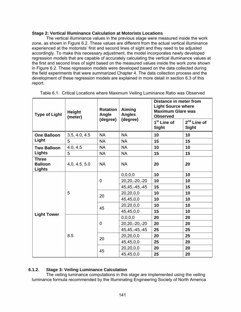
141
Stage 2: Vertical Illuminance Calculation at Motorists Locations The vertical illuminance values in the previous stage were measured inside the work zone, as shown in Figure 6.2. These values are different from the actual vertical illuminance experienced at the motorists’ first and second lines of sight and they need to be adjusted accordingly. To make this necessary adjustment, the model incorporates newly developed regression models that are capable of accurately calculating the vertical illuminance values at the first and second lines of sight based on the measured values inside the work zone shown in Figure 6.2. These regression models were developed based on the data collected during the field experiments that were summarized Chapter 4. The data collection process and the development of these regression models are explained in more detail in section 6.3 of this report.
Table 6.1. Critical Locations where Maximum Veiling Luminance Ratio was Observed
Distance in meter from Light Source where Maximum Glare was Observed Type of Light Height
(meter) Rotation Angle (degree)
Aiming Angles (degree)
1st Line of Sight
2nd Line of Sight
3.5, 4.0, 4.5 NA NA 10 10 One Balloon Light 5 NA NA 15 15
4.0, 4.5 NA NA 10 10 Two Balloon Lights 5 NA NA 15 15 Three Balloon Lights
4,0, 4.5, 5.0 NA NA 20 20
0,0,0,0 10 10 20,20,-20,-20 10 10 0 45,45,-45,-45 15 15 20,20,0,0 10 10
20 45,45,0,0 10 10 20,20,0,0 10 10
5
45 45,45,0,0 15 10 0,0,0,0 20 20 20,20,-20,-20 20 20 0 45,45,-45,-45 25 25 20,20,0,0 20 25
20 45,45,0,0 25 20 20,20,0,0 20 20
Light Tower
8.5
45 45,45,0,0 25 20
6.1.2. Stage 3: Veiling Luminance Calculation The veiling luminance computations in this stage are implemented using the veiling luminance formula recommended by the Illuminating Engineering Society of North America
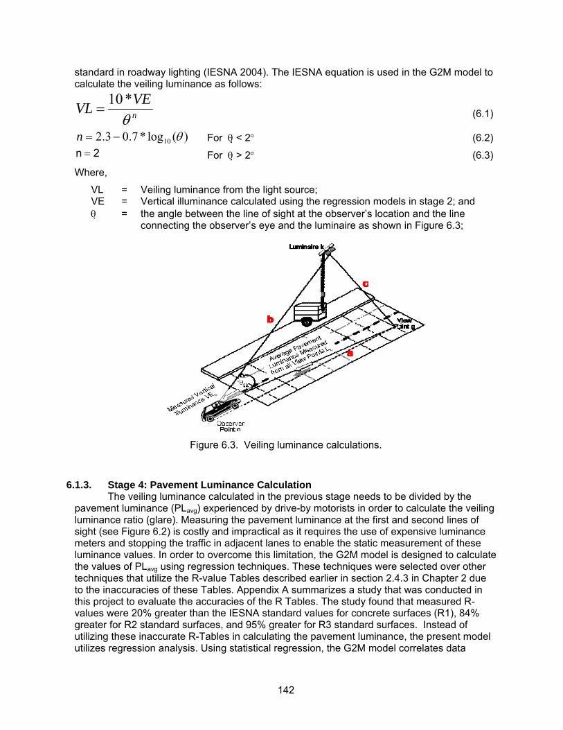
142
standard in roadway lighting (IESNA 2004). The IESNA equation is used in the G2M model to calculate the veiling luminance as follows:
nVEVL
θ*10
= (6.1)
)(log*7.03.2 10 θ−=n For θ < 2° (6.2) 2n = For θ > 2° (6.3)
Where,
VL = Veiling luminance from the light source; VE = Vertical illuminance calculated using the regression models in stage 2; and θ = the angle between the line of sight at the observer’s location and the line
connecting the observer’s eye and the luminaire as shown in Figure 6.3;
Figure 6.3. Veiling luminance calculations.
6.1.3. Stage 4: Pavement Luminance Calculation The veiling luminance calculated in the previous stage needs to be divided by the pavement luminance (PLavg) experienced by drive-by motorists in order to calculate the veiling luminance ratio (glare). Measuring the pavement luminance at the first and second lines of sight (see Figure 6.2) is costly and impractical as it requires the use of expensive luminance meters and stopping the traffic in adjacent lanes to enable the static measurement of these luminance values. In order to overcome this limitation, the G2M model is designed to calculate the values of PLavg using regression techniques. These techniques were selected over other techniques that utilize the R-value Tables described earlier in section 2.4.3 in Chapter 2 due to the inaccuracies of these Tables. Appendix A summarizes a study that was conducted in this project to evaluate the accuracies of the R Tables. The study found that measured R-values were 20% greater than the IESNA standard values for concrete surfaces (R1), 84% greater for R2 standard surfaces, and 95% greater for R3 standard surfaces. Instead of utilizing these inaccurate R-Tables in calculating the pavement luminance, the present model utilizes regression analysis. Using statistical regression, the G2M model correlates data

143
collected during the field experiments on adjacent lanes with actual measurements, thereby creating a predictive model to calculate the glare values without directly measuring them at unsafe locations in open traffic lanes. The data collection process and the development of these regression models are explained in more details in section 6.3.
6.1.4. Stage 5: Veiling Luminance Ratio (Glare) Calculation In this stage, the model is designed to calculate the veiling luminance ratios (V) experienced by drivers approaching the work zone based on the vertical luminance values (VL) calculated in stage 2 and the average pavement luminance (PLavg) calculated in stage 4 in compliance with IESNA recommendations as shown in Equation 6.4.
avgPLVLV = (6.4)
6.2. User Interface The model is implemented as a spread sheet application that runs on Microsoft Excel. The graphical user interface of the model is designed to minimize data input requirements to those that are absolutely necessary to calculate the veiling luminance ratio such as the type and arrangements of lighting equipment on site and vertical illuminance measurements at safe locations inside the work zone. Other data such as pavement luminance are automatically generated and utilized by the model in its various calculation steps. As such, the model includes two types of input data: (1) optional data which provide general and useful information on the project but they are not essential in the computations; and (2) required data which are needed to perform the calculations in the G2M model. First, the optional data input are designed to help resident engineers in recording and tracking the time and location of measurements as well as the weather conditions during the measurements. As shown in Figure 6.4, this optional data include: (1) the project name; (2) the project location; (3) the date of measurements; (4) the type of the construction activity observed; (5) the time of measurements; (6) the weather conditions during the measurements (e.g. cloud conditions, temperature, humidity, and wind speed); and (7) any additional description deemed necessary by the resident engineer. Second, the required data needed to perform the necessary computations of the veiling luminance ratio include: (1) the selection of the type of light (i.e., balloon light or light tower) and its location; and (2) the vertical illuminance measurements obtained by the resident engineer at the critical locations. Based on this required input data, the model performs the necessary computations and displays the calculated veiling luminance ratios as shown in Figure 6.5. A typical user interface session in the model involves the following five main steps.

144
Construction Activity: Paving Bituminous Surfaces Activity
General Information When Taking the Measurment
Time: 11:00 PM
Location of Project: Champaign, IL
Cloud:
Project Name: I-74
Date: Thursday, Nov 9th, 2006
Additional Information: Wind:
Clear
5 mph
Temprature: 33 FHumidity: 70%
Figure 6.4. Optional input cata.
6.2.1. Input Lighting Equipment Data In this first step of the user interface, the resident engineer needs to select the type of construction lighting equipment used on site, as shown in section 1 in Figure 6.5. The two types of lighting equipment that the current model is capable of supporting are light towers and balloon lights which are the most commonly used types of lighting equipment in nighttime highway construction. The model is also designed to generate a customized set of input data fields that are specific to the selected type of lighting equipment. For example, if a balloon light is selected, the model provides the user the option to input the location and height for up to three balloon lights, as shown in Figure 6.6. The input location of the light includes a lateral and longitudinal distances as shown in Figure 6.7.
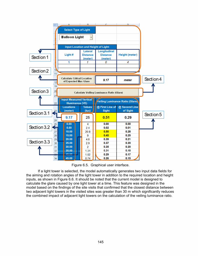
145
Section 1
Section 2
Section 3
Section 4
Section 3.1 Section 5
Section 3.2
Section 3.3
Figure 6.5. Graphical user interface.
If a light tower is selected, the model automatically generates two input data fields for the aiming and rotation angles of the light tower in addition to the required location and height inputs, as shown in Figure 6.6. It should be noted that the current model is designed to calculate the glare caused by one light tower at a time. This feature was designed in the model based on the findings of the site visits that confirmed that the closest distance between two adjacent light towers in the visited sites was greater than 30 m which significantly reduces the combined impact of adjacent light towers on the calculation of the veiling luminance ratio.
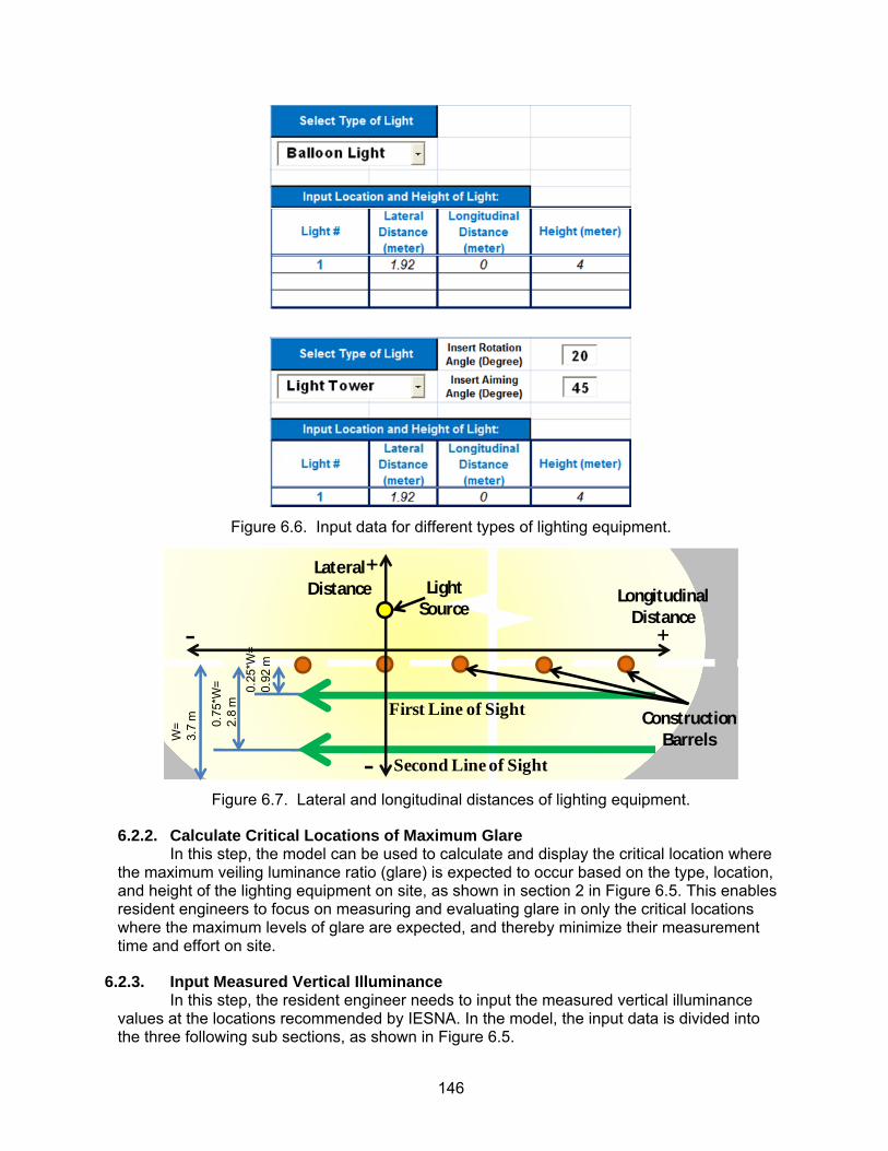
146
Figure 6.6. Input data for different types of lighting equipment.
0.75
*W=
2.8
m
W=
3.7
m First Line of Sight
Second Line of Sight
Light Source
Construction Barrels
Lateral Distance Longitudinal
Distance
-
+
- +
0.25
*W=
0.92
m
Figure 6.7. Lateral and longitudinal distances of lighting equipment.
6.2.2. Calculate Critical Locations of Maximum Glare In this step, the model can be used to calculate and display the critical location where the maximum veiling luminance ratio (glare) is expected to occur based on the type, location, and height of the lighting equipment on site, as shown in section 2 in Figure 6.5. This enables resident engineers to focus on measuring and evaluating glare in only the critical locations where the maximum levels of glare are expected, and thereby minimize their measurement time and effort on site.
6.2.3. Input Measured Vertical Illuminance In this step, the resident engineer needs to input the measured vertical illuminance values at the locations recommended by IESNA. In the model, the input data is divided into the three following sub sections, as shown in Figure 6.5.

147
Section 3.1: In this section, the model calculates and highlights the critical location identified in the previous step to enable the resident engineer to focus on measuring the vertical illuminance at this location where maximum glare is expected. Section 3.2: This section enables the resident engineer to measure vertical illuminance values in various locations in the grid recommended by IESNA in order to further evaluate the veiling luminance ratios in these locations. Section 3.3: This section includes the input fields for the measured vertical illuminance values at the calculated critical location and/or the IESNA recommended locations.
6.2.4. Calculate Veiling Luminance Ratio In this step, the resident engineer can perform the calculation of the veiling luminance ratio (glare) by pressing the button shown in section 4 of Figure 6.5. These computations are performed following the earlier described steps in section 1.1 of this report.
6.2.5. Display Veiling Luminance Ratio (Glare) As shown in section 5 of Figure 6.5, the model displays the calculated veiling luminance ratio (glare) for the first and second lines of sight of the drive-by motorist near the construction site. These results are displayed using four different background colors to represent the severity of the veiling luminance ratio (glare) levels. These four background colors are automatically generated and displayed as follows: (1) white for veiling luminance ratio (V) values less than 0.4; (2) yellow for V values that range between 0.4 and 0.8; (3) orange for V values that range between 0.8 and 1.2; and (4) red for V values that exceed 1.2.
6.3. Regression Models This section presents the development of two types of regression models to support the computational steps in the G2M model described in the previous Chapter. These regression models are designed to calculate (1) the vertical illuminance values experienced by drivers in adjacent lanes to the work zone based on the measured values at safe locations inside the work zone, as shown in Figure 6.2; and (2) the average pavement luminance (PLavg) experienced by drive-by motorists based on the type and arrangement of lighting equipment. These models are developed based on the data collected during the field experiments that were summarized in Chapter 4. The following subsections present the following: (1) the data collection process; (2) an overview of the utilized regression analysis; (3) the development of vertical illuminance regression models, and (4) the development of pavement luminance regression models.
6.3.1. Data Collection As explained in Chapter 4, the field experiments were conducted using a two-lane road to simulate a nighttime work zone in the first lane and an open traffic lane in the second. The simulated work zone layout was set up by formulating the grid of the construction zone into equally spaced points of 5 m. The data collection was performed in three steps: (1) measuring the vertical illuminance (VE) in a safe area next to the construction cones inside the simulated work zone; (2) measuring the vertical illuminance (VE) at the first and second lines of sight for drive-by motorist inside the simulated open traffic lane; and (3) measuring the average pavement luminance (PLavg) experienced by the drive-by motorist. The locations of these measurements were in compliance with the recommendation provided by the Illuminating Engineering Society of North America (IESNA 2004) for isolated traffic conflict areas (partial or non-continuous intersection lighting) due to the similarity between the lighting conditions in these areas and those encountered in nighttime highway construction zones. In particular, IESNA recommends that the area for veiling luminance ratio (glare) measurements should

148
extend from one mounting height of the light pole in front of the light to 45 m before that point and the grid increment should be 5 m as explained in Chapter 4 and as shown in Figure 6.8.
Light Source
45m
12391011VL2,1
VL2,2
VL3,1
VL3,2
5 m
VL1,1 START
VL1,2
5m
Veiling luminance
Grid
VL11,1
VL11,2START
END
END
0.25*W= 0.92 m
0.75*W= 2.8 mW=
3.7 m
First Line of Sight
Second Line of Sight
Figure 6.8. Veiling luminance grid locations recommended by IESNA.
6.3.1.1. Vertical Illuminance Measurements inside the Work Zone Vertical illuminance values were measured by the research team inside the work zone to simulate the measurements that a resident engineer can safely take within the work zone and without interrupting the flow of traffic in adjacent lanes, as shown in Figure 6.9. The longitudinal spacing between these measurement locations was selected in compliance with the locations recommended by IESNA/ANSI RP-8-00 when measuring the VE experienced by the traveling public, as shown in the grid in Figure 6.9. Each measurement was taken using an illuminance meter while standing inside the work zone in a safe area that is close to the construction cones. The illuminance meter was positioned at a height of 1.45 m above the street level to simulate the height of the line of sight for a drive-by motorist as recommended by IESNA/ANSI RP-8-00 (IESNA 2004). The first measurement was taken at point 1 (see Figure 6.2) then the next were taken at 5 m intervals along a safe line inside the construction site (i.e., next to the construction cones) until the end of the shown grid.
45m
12391011
5 m START
5mVeiling luminance
Grid (IESNA)
VE1
END
0.25*W= 0.92 m
0.75*W= 2.8 mW=
3.7 m
First Line of Sight
Second Line of Sight
Light Source
Veiling luminance Grid (Research Team)
VE2VE11VE10 VE9 VE3
Figure 6.9. Veiling luminance grid locations in field tests.
6.3.1.2. Vertical Illuminance Measurements at First and Second Lines of Sight Vertical illuminance values were measured by the research team at the first and second lines of sight in the open traffic lane (see Figure 6.9) to calculate the vertical illuminance experienced by drive-by motorists at these locations. The locations for measuring and calculating the veiling luminance were selected based on the IESNA/ANSI RP-8-00
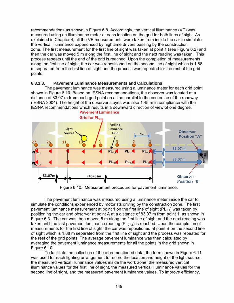
149
recommendations as shown in Figure 6.8. Accordingly, the vertical illuminance (VE) was measured using an illuminance meter at each location on the grid for both lines of sight. As explained in Chapter 4, all the VE measurements were taken from inside the car to simulate the vertical illuminance experienced by nighttime drivers passing by the construction zone. The first measurement for the first line of sight was taken at point 1 (see Figure 6.2) and then the car was moved 5 m along the first line of sight and the next reading was taken. This process repeats until the end of the grid is reached. Upon the completion of measurements along the first line of sight, the car was repositioned on the second line of sight which is 1.88 m separated from the first line of sight and the process was repeated for the rest of the grid points. 6.3.1.3. Pavement Luminance Measurements and Calculations The pavement luminance was measured using a luminance meter for each grid point shown in Figure 6.10. Based on IESNA recommendations, the observer was located at a distance of 83.07 m from each grid point on a line parallel to the centerline of the roadway (IESNA 2004). The height of the observer’s eyes was also 1.45 m in compliance with the IESNA recommendations which results in a downward direction of view of one degree.
Figure 6.10. Measurement procedure for pavement luminance.
The pavement luminance was measured using a luminance meter inside the car to simulate the conditions experienced by motorists driving by the construction zone. The first pavement luminance measurement at point 1 on the first line of sight (PL1,1) was taken by positioning the car and observer at point A at a distance of 83.07 m from point 1, as shown in Figure 6.3. The car was then moved 5 m along the first line of sight and the next reading was taken until the last pavement luminance reading (PL27,1) is reached. Upon the completion of measurements for the first line of sight, the car was repositioned at point B on the second line of sight which is 1.88 m separated from the first line of sight and the process was repeated for the rest of the grid points. The average pavement luminance was then calculated by averaging the pavement luminance measurements for all the points in the grid shown in Figure 6.10. To facilitate the collection of the aforementioned data, the form shown in Figure 6.11 was used for each lighting arrangement to record the location and height of the light source, the measured vertical illuminance values inside the work zone, the measured vertical illuminance values for the first line of sight, the measured vertical illuminance values for the second line of sight, and the measured pavement luminance values. To improve efficiency,
150
the data collection procedure was performed by three researchers who preformed the following tasks at each measurement location: (1) the first researcher took the measurements; (2) the second recorded the measurements using the form shown in Figure 6.4; and (3) the third helped with identifying the 83.07 m location that is in front of the car for the pavement luminance measurements requirement.
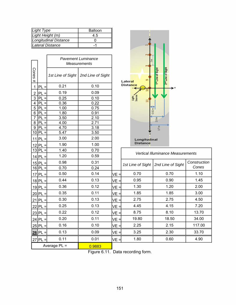
151
Balloon4.50-1
1st Line of Sight 2nd Line of Sight
1 PL = 0.21 0.10
2 PL = 0.19 0.093 PL = 0.25 0.104 PL = 0.36 0.225 PL = 1.00 0.756 PL = 1.80 0.917 PL = 3.50 2.108 PL = 4.00 2.719 PL = 4.70 3.18
10 PL = 5.47 3.5011 PL = 3.00 2.00
12 PL = 1.90 1.0013 PL = 1.40 0.7014 PL = 1.20 0.59
15 PL = 0.98 0.3116 PL = 0.70 0.2417 PL = 0.50 0.14 VE = 0.70 0.70 1.10
18 PL = 0.44 0.13 VE = 0.95 0.90 1.45
19 PL = 0.36 0.12 VE = 1.30 1.20 2.00
20 PL = 0.35 0.11 VE = 1.85 1.85 3.00
21 PL = 0.30 0.13 VE = 2.75 2.75 4.50
22 PL = 0.25 0.13 VE = 4.45 4.15 7.20
23 PL = 0.22 0.12 VE = 8.75 8.10 13.70
24 PL = 0.20 0.11 VE = 19.80 18.50 34.00
25 PL = 0.16 0.10 VE = 2.25 2.15 117.00
26 PL = 0.13 0.09 VE = 3.25 2.30 33.70
27 PL = 0.11 0.01 VE = 1.80 0.60 4.90
0.9883Average PL =
Longitudinal Distance
1st Line of Sight
Vertical Illuminance Measurements
Construction Cones2nd Line of Sight
Cones #
Pavement Luminance Measurements
Light TypeLight Height (m)
Lateral Distance
Figure 6.11. Data recording form.

152
6.3.2. Overview of Regression Analysis The main purpose of regression analysis is to quantify the relationship between several independent or predictor variables and a dependent variable. The following two sections discuss: (1) the type of regression analysis used in this study to predict the dependent variables (i.e., vertical illuminance at first and second lines of sight and the average pavement luminance); and (2) the regression analysis procedure and results. 6.3.2.1. High-Level and Stepwise Regression Analysis The high-level regression analysis is a combination of factorial and polynomial regression. The factorial regression analysis presents the relationship between the dependent variable and the possible products of the independent variables (StatSoft 2007). For example a factorial regression formula for two independent variables can be given by the following equation:
Y = a0 + a1 O + a2 P + a3 (O*P) (6.5)
Where; a1, a2, and a3 represent the independent contributions of each term in the formula to the prediction of the dependent variable “Y” (StateSoft 2007; Cryer and Miller 1991).
The polynomial regression analysis explains the relationship between the dependent variable and the higher-order effect of the independent variables. This analysis does not provide an interaction between the independent variables in the equation (StatSoft 2007). For example, the relationship between Y and two independent variables O and P can be presented by the following polynomial regression formula:
Y = a0 + a1 O + a2 O2 + a3 P + a4 P2 (6.6)
The high-level regression analysis provides a combination between the two aforementioned regression analyses. It considers several designs in the relationship: (1) the first-order of the independent variable; (2) the higher-order of the independent variables; and (3) the interaction between all possible combinations (StatSoft 2007). For example, the independent variables O and P present the relationship with the dependent variable Y using the following high-level regression equation:
Y = a0 + a1 O + a2 O2 + a3 P + a4 P2 + a5 (O * P) + a6 (O * P2) + a7 (P * O2) + a8(O2*P2) + a8 (O * O2) + a9 (P * P2) (6.7)
The type of interaction between the variables in equation 2.3 is known as 2-way interaction (StatSoft 2007). Further analysis can also be accomplished by applying a 3-way interaction between the independent variables. This high level of interactions will help in exploring more combinations between the independent variable (StatSoft 2007). For example, a 3-way interaction of the same variables in equation (6.7) will be as follows:
Y = a0 + a1 O + a2 O2 + a3 P + a4 P2 + a5 (O * P) + a6 (O * P2) + a7 (P * O2) + a8 (O2*P2) + a8 (O * O2) + a9 (P * P2) + a10 (P*O*P2) + a11 (P*O*O2) + a12 (P*P2*O2) + a13 (O*P2*O2) (6.8)
High-level regression analysis with 3-way interaction might generate a large number of terms that are not fully capable of predicting the dependent variable (Y). However, these terms might affect the results and lower the prediction capability of the suggested regression model. In order to overcome this problem, “step wise” regression techniques are applied in this analysis

153
to eliminate any terms that do not contribute significantly in explaining the dependent variable (Kovoor and Nandagiri 2007; StatSoft 2007; Cryer and Miller 1991).
6.3.2.2. Regression Analysis Procedure and Results The analyses explained in the following sections adapted the high-level regression analyses and were evaluated using Sagata Regression Pro software. The software has the capability to perform high-level regression analysis with a 3-way interaction of the independent variables. In addition, the “step wise” regression technique was applied so as to generate the best combination of terms which contribute significantly in explaining the dependent variable. For each of the developed regression models in this study, the regression procedure and results are summarized in five main steps:
(1) Correlation: The independent variables are tested to ensure that they are not dependent on each other. This is accomplished by calculating the correlation coefficient. In case there are more than two variables, a correlation matrix is generated to show the correlation between the tested variables. The value of a correlation coefficient can vary from -1 to +1, where the coefficient indicates a perfect negative correlation for -1 and a perfect positive correlation for +1. A correlation of 0 means there is no relationship between the two variables.
(2) Summary of statistics: In this section, two criteria are presented for each regression model: (i) the coefficient of determination (R2) which indicates how close the match is between the predictions from the model and the measured values from the field tests. R2 values range from 0 to 1 where values close to 1 indicate a good match and those close to 0 indicate a poor match; and (ii) R2-adj which has similar interpretation as R2 but seeks to circumvent some of the limitations of R2 (Sagata Regression Pro 2004).
(3) Analysis of Variance (ANOVA): This analysis shows how much of the analyzed data variation is explained by the developed model.
(4) Coefficients Tables: This table presents: (i) the final generated terms of the regression model; and (ii) the coefficient estimates for each term.
(5) Residuals Table: This section presents a table that shows: (i) the predicted values generated by the model; (ii) the observed values based on the collected data; (iii) the residuals; and (iv) the percentage of the residuals compared to the measured values from the field tests.
6.3.3. Vertical Illuminance Regression Models A number of regression models were developed to predict the vertical illuminance values experienced by drivers in lanes adjacent to the work zone based on the measured values at safe locations inside the work zone. The following sections describe the development of these models for four commonly used lighting arrangements in nighttime construction sites: one balloon light, two balloon lights, three balloon lights, and one light tower. 6.3.3.1. One Balloon Light In this analysis, the dependent variable of the regression model is the vertical illuminance values at the first and second lines of sight. The independent variables are: (1) the vertical illuminance values measured by a resident engineer at a safe zone inside the work zone (WZ); and (2) the height of the balloon light (H). The correlation between the two independent variables WZ and H was measured and was found to be -0.055 which emphasizes that there is no correlation between these two independent variables.
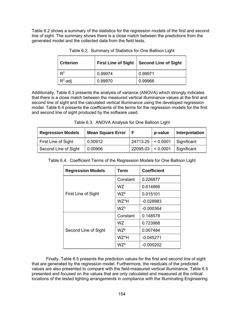
154
Table 6.2 shows a summary of the statistics for the regression models of the first and second line of sight. The summary shows there is a close match between the predictions from the generated model and the collected data from the field tests.
Table 6.2. Summary of Statistics for One Balloon Light
Criterion First Line of Sight Second Line of Sight
R2 0.99974 0.99971
R2-adj 0.99970 0.99966
Additionally, Table 6.3 presents the analysis of variance (ANOVA) which strongly indicates that there is a close match between the measured vertical illuminance values at the first and second line of sight and the calculated vertical illuminance using the developed regression model. Table 6.4 presents the coefficients of the terms for the regression models for the first and second line of sight produced by the software used.
Table 6.3. ANOVA Analysis for One Balloon Light
Regression Models Mean Square Error F p-value Interpretation
First Line of Sight 0.00912 24713.25 < 0.0001 Significant
Second Line of Sight 0.00906 22095.03 < 0.0001 Significant
Table 6.4. Coefficient Terms of the Regression Models for One Balloon Light
Regression Models Term Coefficient
Constant 0.226877
WZ 0.614866
WZ² 0.015101
WZ*H -0.028983
First Line of Sight
WZ³ -0.000364
Constant 0.148578
WZ 0.723988
WZ² 0.007484
WZ*H -0.045271
Second Line of Sight
WZ³ -0.000202 Finally, Table 6.5 presents the prediction values for the first and second line of sight that are generated by the regression model. Furthermore, the residuals of the predicted values are also presented to compare with the field-measured vertical illuminance. Table 6.5 presented and focused on the values that are only calculated and measured at the critical locations of the tested lighting arrangements in compliance with the Illuminating Engineering
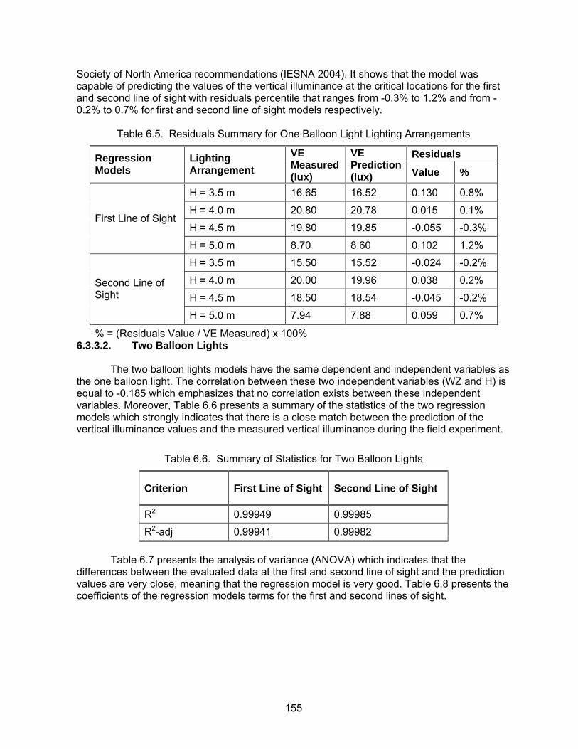
155
Society of North America recommendations (IESNA 2004). It shows that the model was capable of predicting the values of the vertical illuminance at the critical locations for the first and second line of sight with residuals percentile that ranges from -0.3% to 1.2% and from -0.2% to 0.7% for first and second line of sight models respectively.
Table 6.5. Residuals Summary for One Balloon Light Lighting Arrangements
Residuals Regression Models
Lighting Arrangement
VE Measured (lux)
VE Prediction (lux) Value %
H = 3.5 m 16.65 16.52 0.130 0.8%
H = 4.0 m 20.80 20.78 0.015 0.1%
H = 4.5 m 19.80 19.85 -0.055 -0.3% First Line of Sight
H = 5.0 m 8.70 8.60 0.102 1.2%
H = 3.5 m 15.50 15.52 -0.024 -0.2%
H = 4.0 m 20.00 19.96 0.038 0.2%
H = 4.5 m 18.50 18.54 -0.045 -0.2% Second Line of Sight
H = 5.0 m 7.94 7.88 0.059 0.7%
% = (Residuals Value / VE Measured) x 100% 6.3.3.2. Two Balloon Lights The two balloon lights models have the same dependent and independent variables as the one balloon light. The correlation between these two independent variables (WZ and H) is equal to -0.185 which emphasizes that no correlation exists between these independent variables. Moreover, Table 6.6 presents a summary of the statistics of the two regression models which strongly indicates that there is a close match between the prediction of the vertical illuminance values and the measured vertical illuminance during the field experiment.
Table 6.6. Summary of Statistics for Two Balloon Lights
Criterion First Line of Sight Second Line of Sight
R2 0.99949 0.99985
R2-adj 0.99941 0.99982 Table 6.7 presents the analysis of variance (ANOVA) which indicates that the differences between the evaluated data at the first and second line of sight and the prediction values are very close, meaning that the regression model is very good. Table 6.8 presents the coefficients of the regression models terms for the first and second lines of sight.
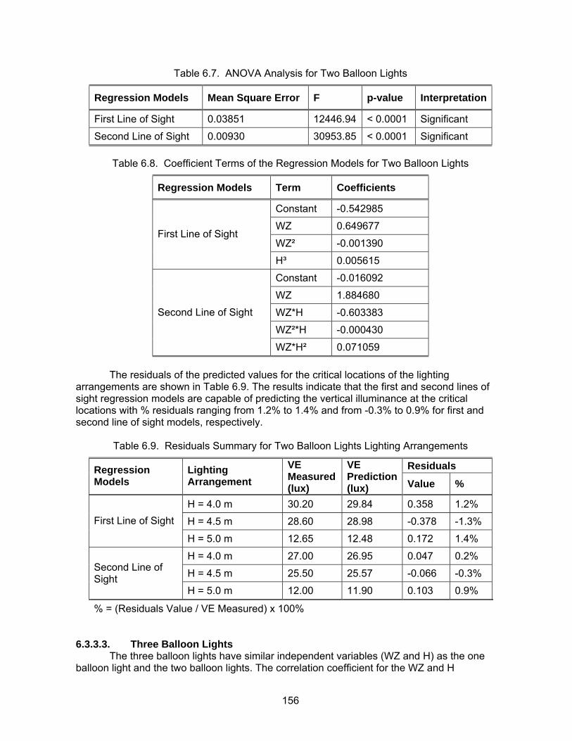
156
Table 6.7. ANOVA Analysis for Two Balloon Lights
Regression Models Mean Square Error F p-value Interpretation
First Line of Sight 0.03851 12446.94 < 0.0001 Significant
Second Line of Sight 0.00930 30953.85 < 0.0001 Significant
Table 6.8. Coefficient Terms of the Regression Models for Two Balloon Lights
Regression Models Term Coefficients
Constant -0.542985
WZ 0.649677
WZ² -0.001390 First Line of Sight
H³ 0.005615
Constant -0.016092
WZ 1.884680
WZ*H -0.603383
WZ²*H -0.000430
Second Line of Sight
WZ*H² 0.071059
The residuals of the predicted values for the critical locations of the lighting arrangements are shown in Table 6.9. The results indicate that the first and second lines of sight regression models are capable of predicting the vertical illuminance at the critical locations with % residuals ranging from 1.2% to 1.4% and from -0.3% to 0.9% for first and second line of sight models, respectively.
Table 6.9. Residuals Summary for Two Balloon Lights Lighting Arrangements
Residuals Regression Models
Lighting Arrangement
VE Measured (lux)
VE Prediction (lux) Value %
H = 4.0 m 30.20 29.84 0.358 1.2%
H = 4.5 m 28.60 28.98 -0.378 -1.3% First Line of Sight
H = 5.0 m 12.65 12.48 0.172 1.4%
H = 4.0 m 27.00 26.95 0.047 0.2%
H = 4.5 m 25.50 25.57 -0.066 -0.3% Second Line of Sight
H = 5.0 m 12.00 11.90 0.103 0.9%
% = (Residuals Value / VE Measured) x 100% 6.3.3.3. Three Balloon Lights The three balloon lights have similar independent variables (WZ and H) as the one balloon light and the two balloon lights. The correlation coefficient for the WZ and H
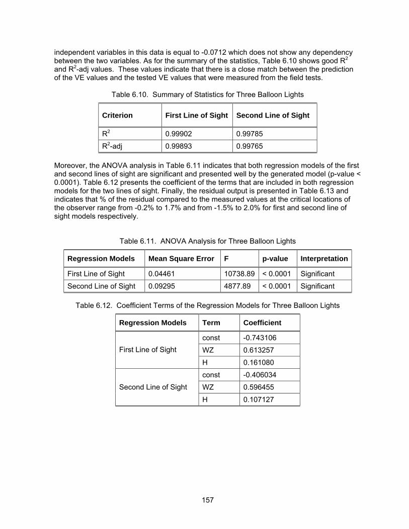
157
independent variables in this data is equal to -0.0712 which does not show any dependency between the two variables. As for the summary of the statistics, Table 6.10 shows good R2 and R2-adj values. These values indicate that there is a close match between the prediction of the VE values and the tested VE values that were measured from the field tests.
Table 6.10. Summary of Statistics for Three Balloon Lights
Criterion First Line of Sight Second Line of Sight
R2 0.99902 0.99785
R2-adj 0.99893 0.99765
Moreover, the ANOVA analysis in Table 6.11 indicates that both regression models of the first and second lines of sight are significant and presented well by the generated model (p-value < 0.0001). Table 6.12 presents the coefficient of the terms that are included in both regression models for the two lines of sight. Finally, the residual output is presented in Table 6.13 and indicates that % of the residual compared to the measured values at the critical locations of the observer range from -0.2% to 1.7% and from -1.5% to 2.0% for first and second line of sight models respectively.
Table 6.11. ANOVA Analysis for Three Balloon Lights
Regression Models Mean Square Error F p-value Interpretation
First Line of Sight 0.04461 10738.89 < 0.0001 Significant
Second Line of Sight 0.09295 4877.89 < 0.0001 Significant
Table 6.12. Coefficient Terms of the Regression Models for Three Balloon Lights
Regression Models Term Coefficient
const -0.743106
WZ 0.613257 First Line of Sight
H 0.161080
const -0.406034
WZ 0.596455 Second Line of Sight
H 0.107127
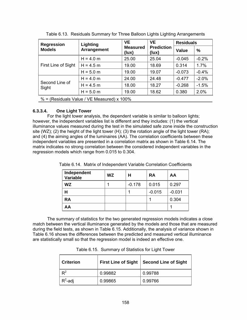
158
Table 6.13. Residuals Summary for Three Balloon Lights Lighting Arrangements
Residuals Regression Models
Lighting Arrangement
VE Measured (lux)
VE Prediction (lux) Value %
H = 4.0 m 25.00 25.04 -0.045 -0.2% H = 4.5 m 19.00 18.69 0.314 1.7% First Line of Sight H = 5.0 m 19.00 19.07 -0.073 -0.4% H = 4.0 m 24.00 24.48 -0.477 -2.0% H = 4.5 m 18.00 18.27 -0.268 -1.5% Second Line of
Sight H = 5.0 m 19.00 18.62 0.380 2.0%
% = (Residuals Value / VE Measured) x 100%
6.3.3.4. One Light Tower For the light tower analysis, the dependent variable is similar to balloon lights; however, the independent variables list is different and they includes: (1) the vertical illuminance values measured during the test in the simulated safe zone inside the construction site (WZ); (2) the height of the light tower (H); (3) the rotation angle of the light tower (RA); and (4) the aiming angles of the luminaires (AA). The correlation coefficients between these independent variables are presented in a correlation matrix as shown in Table 6.14. The matrix indicates no strong correlation between the considered independent variables in the regression models which range from 0.015 to 0.304.
Table 6.14. Matrix of Independent Variable Correlation Coefficients
Independent Variable WZ H RA AA
WZ 1 -0.178 0.015 0.297
H 1 -0.015 -0.031
RA 1 0.304
AA 1
The summary of statistics for the two generated regression models indicates a close match between the vertical illuminance generated by the models and those that are measured during the field tests, as shown in Table 6.15. Additionally, the analysis of variance shown in Table 6.16 shows the differences between the predicted and measured vertical illuminance are statistically small so that the regression model is indeed an effective one.
Table 6.15. Summary of Statistics for Light Tower
Criterion First Line of Sight Second Line of Sight
R2 0.99882 0.99788
R2-adj 0.99865 0.99766
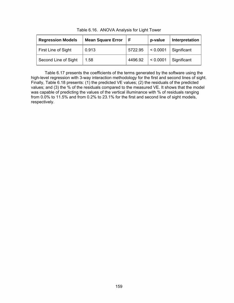
159
Table 6.16. ANOVA Analysis for Light Tower
Regression Models Mean Square Error F p-value Interpretation
First Line of Sight 0.913 5722.95 < 0.0001 Significant
Second Line of Sight 1.58 4496.92 < 0.0001 Significant
Table 6.17 presents the coefficients of the terms generated by the software using the high-level regression with 3-way interaction methodology for the first and second lines of sight. Finally, Table 6.18 presents: (1) the predicted VE values; (2) the residuals of the predicted values; and (3) the % of the residuals compared to the measured VE. It shows that the model was capable of predicting the values of the vertical illuminance with % of residuals ranging from 0.0% to 11.5% and from 0.2% to 23.1% for the first and second line of sight models, respectively.

160
Table 6.17. Coefficient Terms of the Regression Models for Light Tower
Regression Models Term Coefficients
Constant 0.123216
WZ 0.494408
WZ*H 0.013241
WZ*RA 0.022795
WZ*AA -0.012059
WZ³ 0.000004
AA³ -0.000008
WZ²*H -0.000264
WZ²*RA -0.000043
WZ*H*RA -0.001130
WZ*RA² -0.000146
WZ*RA*AA -0.000144
First Line of Sight
WZ*AA² 0.000328
Constant 0.303237
WZ 0.482967
WZ*RA 0.022490
WZ*AA -0.018932
H*AA 0.003446
WZ²*RA -0.000016
WZ*H*RA -0.000896
WZ*RA² -0.000159
WZ*RA*AA -0.000138
Second Line of Sight
WZ*AA² 0.000432
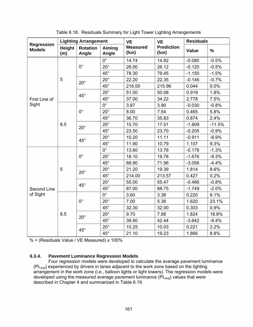
161
Table 6.18. Residuals Summary for Light Tower Lighting Arrangements
Lighting Arrangement Residuals Regression Models Height
(m) Rotation Angle
Aiming Angle
VE Measured (lux)
VE Prediction (lux) Value %
0° 14.74 14.82 -0.080 -0.5% 20° 26.00 26.12 -0.120 -0.5% 0° 45° 78.30 79.45 -1.150 -1.5% 20° 22.20 22.35 -0.146 -0.7%
20° 45° 216.00 215.96 0.044 0.0% 20° 51.00 50.08 0.919 1.8%
5
45° 45° 37.00 34.22 2.778 7.5% 0° 3.87 3.90 -0.030 -0.8% 20° 8.00 7.54 0.465 5.8% 0° 45° 36.70 35.83 0.874 2.4% 20° 15.70 17.51 -1.809 -11.5%
20° 45° 23.50 23.70 -0.205 -0.9% 20° 10.20 11.11 -0.911 -8.9%
First Line of Sight
8.5
45° 45° 11.90 10.79 1.107 9.3% 0° 13.60 13.78 -0.178 -1.3% 20° 18.10 19.78 -1.676 -9.3% 0° 45° 68.90 71.96 -3.056 -4.4% 20° 21.20 19.39 1.814 8.6%
20° 45° 214.00 213.57 0.427 0.2% 20° 55.00 55.47 -0.466 -0.8%
5
45° 45° 87.00 88.75 -1.749 -2.0% 0° 3.60 3.38 0.220 6.1% 20° 7.00 5.38 1.620 23.1% 0° 45° 32.30 32.00 0.303 0.9% 20° 9.70 7.88 1.824 18.8%
20° 45° 38.80 42.44 -3.642 -9.4% 20° 10.25 10.03 0.221 2.2%
Second Line of Sight
8.5
45° 45° 21.10 19.23 1.866 8.8%
% = (Residuals Value / VE Measured) x 100%
6.3.4. Pavement Luminance Regression Models Four regression models were developed to calculate the average pavement luminance (PLavg) experienced by drivers in lanes adjacent to the work zone based on the lighting arrangement in the work zone (i.e., balloon lights or light towers). The regression models were developed using the measured average pavement luminance (PLavg) values that were described in Chapter 4 and summarized in Table 6.19.
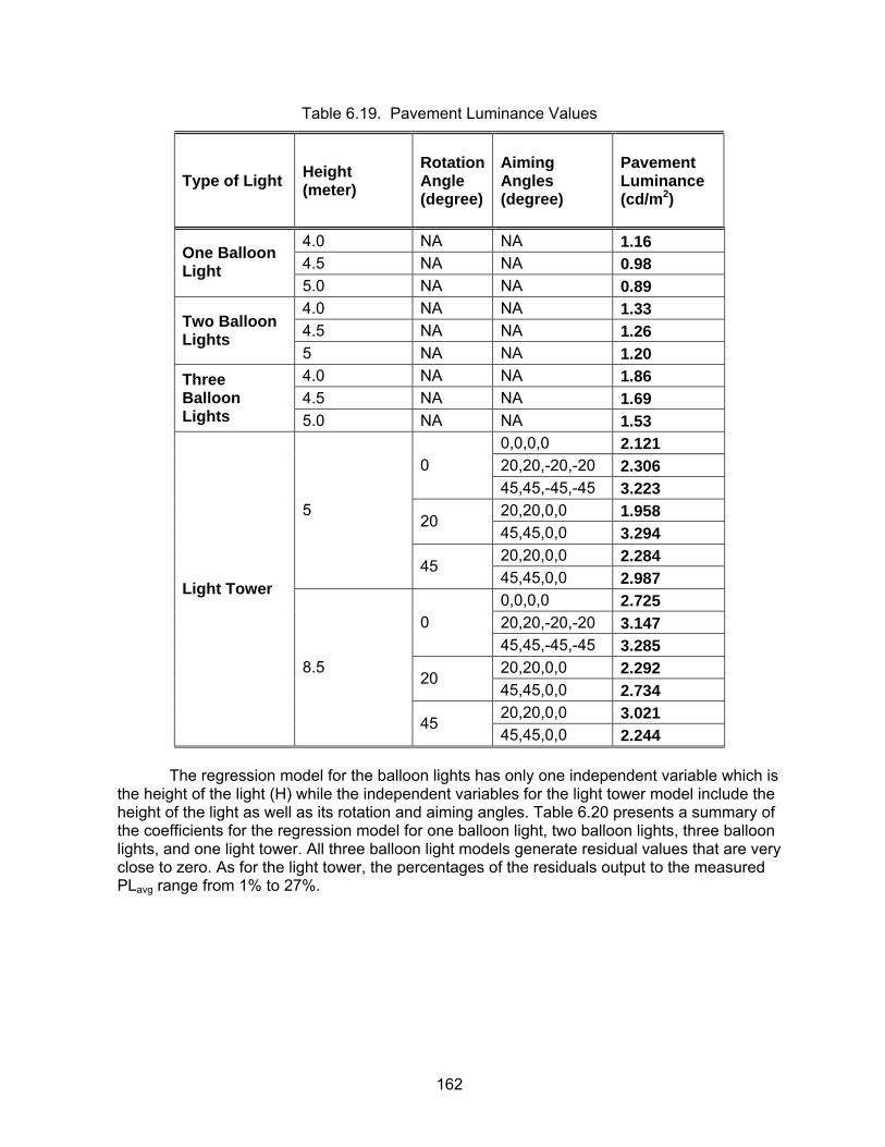
162
Table 6.19. Pavement Luminance Values
Type of Light Height (meter)
Rotation Angle (degree)
Aiming Angles (degree)
Pavement Luminance (cd/m2)
4.0 NA NA 1.16 4.5 NA NA 0.98 One Balloon
Light 5.0 NA NA 0.89 4.0 NA NA 1.33 4.5 NA NA 1.26 Two Balloon
Lights 5 NA NA 1.20 4.0 NA NA 1.86 4.5 NA NA 1.69
Three Balloon Lights 5.0 NA NA 1.53
0,0,0,0 2.121 20,20,-20,-20 2.306 0 45,45,-45,-45 3.223 20,20,0,0 1.958 20 45,45,0,0 3.294 20,20,0,0 2.284
5
45 45,45,0,0 2.987 0,0,0,0 2.725 20,20,-20,-20 3.147 0 45,45,-45,-45 3.285 20,20,0,0 2.292 20 45,45,0,0 2.734 20,20,0,0 3.021
Light Tower
8.5
45 45,45,0,0 2.244
The regression model for the balloon lights has only one independent variable which is the height of the light (H) while the independent variables for the light tower model include the height of the light as well as its rotation and aiming angles. Table 6.20 presents a summary of the coefficients for the regression model for one balloon light, two balloon lights, three balloon lights, and one light tower. All three balloon light models generate residual values that are very close to zero. As for the light tower, the percentages of the residuals output to the measured PLavg range from 1% to 27%.
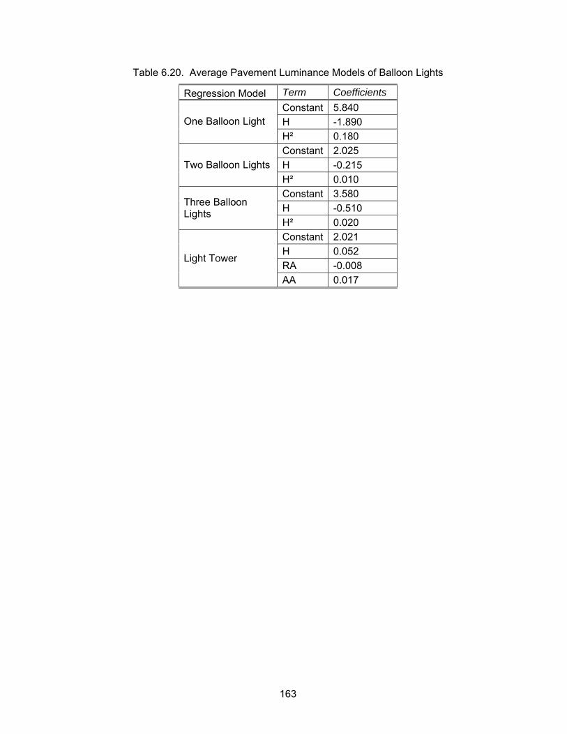
163
Table 6.20. Average Pavement Luminance Models of Balloon Lights
Regression Model Term Coefficients Constant 5.840 H -1.890 One Balloon Light H² 0.180 Constant 2.025 H -0.215 Two Balloon Lights H² 0.010 Constant 3.580 H -0.510 Three Balloon
Lights H² 0.020 Constant 2.021 H 0.052 RA -0.008
Light Tower
AA 0.017

164
CHAPTER 7 MAXIMUM ALLOWABLE LEVELS OF VEILING LUMINANCE RATIO 7. 2 Based on the evaluations and experiments conducted in the field experiments, recommendations are presented in this chapter on the maximum allowable level of veiling luminance ratio that can be tolerated by nighttime motorists. Existing studies and recommendations focused on two main sources of glare that are caused by roadway lighting and by the headlights of opposite traffic vehicles. The following sections summarize these findings.
7.1. Glare from Roadway Lighting IESNA recommends the use of the ratio of maximum veiling luminance to the average pavement luminance of 0.4 to control glare in roadway lighting design (IESNA 2004). This ratio can be considered applicable to highway work zones due to the similarities in design criteria, parameters, and designers concerns in both cases. It should be noted that this ratio can be slightly relaxed to account for the temporary nature of work zone lighting.
7.2. Glare from Headlights of Opposite Traffic Vehicles A study by Schieber (1998) was conducted to quantify disabling glare from upper and lower beams of daytime running lamps (DRLs) under different lighting conditions ranging from dawn to dusk. This study was based on four main assumptions: (1) the minimum light intensity value for the DRL is 1,500 cd and the maximum is 7,000 cd according to the Federal Motor Vehicle Safety Standards and 10,000 cd was also considered in case of over voltage problems; (2) viewing distances of 20 m through 100 m between the motorist and the headlight of an opposite traffic vehicle ; (3) a two-lane road with 3.7 m lane widths; and (4) the pavement luminance for the driver is 1 cd/m2 for nighttime driving lighting condition. Based on these assumptions, Schieber (1998) calculated and summarized the veiling luminance ratio (glare) experienced by the traveling public from headlights of opposite traffic, as shown in Table 7.1.
Table 7.1. Veiling Luminance Ratio for 1,500; 7,000; and 10,000 cd Daytime Running Lights
(Schieber 1998)
Distance VL-Ratio (1,500 cd) VL-Ratio (7,000 cd) VL-Ratio (10,000 cd)
- 20 m 0.95 4.42 5.8 - 40 m 0.93 4.3 5.7 - 60 m 0.93 4.33 5.7 - 80 m 0.87 4.16 5.7 - 100 m 0.93 4.32 5.7
Schieber (1998) reported that significant disabling glare was experienced by drivers when the VL-Ratio value exceeded 1.0. Accordingly, the results in Table 7.1 illustrates that daylight running lights intensity of 7,000 cd and 10,000 cd represent a potentially significant source of glare to opposite drivers at nighttime driving conditions since the veiling luminance ratio was found to be greater than 1.0 (Schieber 1998). The Schieber study (1998) was based on a proposed grid of 100 m long with equal distances of 20 m which does not comply with the IESNA grid requirements (IESNA 2004). Accordingly, the research team conducted an experimental study of the veiling luminance ratio (glare) that is experienced by the traveling public from the headlight of opposite traffic while
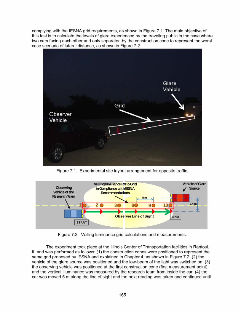
165
complying with the IESNA grid requirements, as shown in Figure 7.1. The main objective of this test is to calculate the levels of glare experienced by the traveling public in the case where two cars facing each other and only separated by the construction cone to represent the worst case scenario of lateral distance, as shown in Figure 7.2.
Figure 7.1. Experimental site layout arrangement for opposite traffic.
1 2 3 9 10
5 m
Veiling luminance Ratio Grid in Compliance with IESNA
Recommendations
END
START
Vehicle of Glare SourceObserving
Vehicle of the Research Team
2.4 m
Observer Line of Sight
8
Figure 7.2. Veiling luminance grid calculations and measurements.
The experiment took place at the Illinois Center of Transportation facilities in Rantoul, IL and was performed as follows: (1) the construction cones were positioned to represent the same grid proposed by IESNA and explained in Chapter 4, as shown in Figure 7.2; (2) the vehicle of the glare source was positioned and the low-beam of the light was switched on; (3) the observing vehicle was positioned at the first construction cone (first measurement point) and the vertical illuminance was measured by the research team from inside the car; (4) the car was moved 5 m along the line of sight and the next reading was taken and continued until
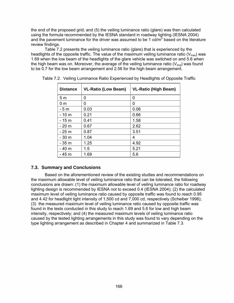
166
the end of the proposed grid; and (5) the veiling luminance ratio (glare) was then calculated using the formula recommended by the IESNA standard in roadway lighting (IESNA 2004) and the pavement luminance for the driver was assumed to be 1 cd/m2 based on the literature review findings. Table 7.2 presents the veiling luminance ratio (glare) that is experienced by the headlights of the opposite traffic. The value of the maximum veiling luminance ratio (Vmax) was 1.69 when the low beam of the headlights of the glare vehicle was switched on and 5.6 when the high beam was on. Moreover, the average of the veiling luminance ratio (Vavg) was found to be 0.7 for the low beam arrangement and 2.56 for the high beam arrangement.
Table 7.2. Veiling Luminance Ratio Experienced by Headlights of Opposite Traffic
Distance VL-Ratio (Low Beam) VL-Ratio (High Beam)
5 m 0 0 0 m 0 0 - 5 m 0.03 0.06 - 10 m 0.21 0.66 - 15 m 0.41 1.58 - 20 m 0.67 2.62 - 25 m 0.87 3.51 - 30 m 1.04 4 - 35 m 1.25 4.92 - 40 m 1.5 5.21 - 45 m 1.69 5.6
7.3. Summary and Conclusions Based on the aforementioned review of the existing studies and recommendations on the maximum allowable level of veiling luminance ratio that can be tolerated, the following conclusions are drawn: (1) the maximum allowable level of veiling luminance ratio for roadway lighting design is recommended by IESNA not to exceed 0.4 (IESNA 2004); (2) the calculated maximum level of veiling luminance ratio caused by opposite traffic was found to reach 0.95 and 4.42 for headlight light intensity of 1,500 cd and 7,000 cd, respectively (Scheiber 1998); (3) the measured maximum level of veiling luminance ratio caused by opposite traffic was found in the tests conducted in this study to reach 1.69 and 5.6 for low and high beam intensity, respectively; and (4) the measured maximum levels of veiling luminance ratio caused by the tested lighting arrangements in this study was found to vary depending on the type lighting arrangement as described in Chapter 4 and summarized in Table 7.3.

167
Table 7.3. Vmax Values for Tested Lighting Arrangements
Type of Light Height in meter Rotation Angle Aiming Angles Vmax
3.5 NA NA 0.64 4.0 NA NA 0.50 4.5 NA NA 0.45
One Balloon Light
5 NA NA 0.37 4.0 NA NA 0.54 4.5 NA NA 0.44 Two Balloon Lights 5 NA NA 0.34 4.0 NA NA 0.56 4.5 NA NA 0.40 Three Balloon Lights 5.0 NA NA 0.37
0,0,0,0 0.11 20,20,-20,-20 0.18 0 45,45,-45,-45 0.77 20,20,0,0 0.18
20 45,45,0,0 1.02 20,20,0,0 0.35
5
45 45,45,0,0 0.39 0,0,0,0 0.03 20,20,-20,-20 0.05 0 45,45,-45,-45 0.35 20,20,0,0 0.14
20 45,45,0,0 0.27 20,20,0,0 0.07
Light Tower
8.5
45 45,45,0,0 0.16
Nite Lite 3.5 NA NA 0.84

168
CHAPTER 8 CONCLUSIONS AND FUTURE RESEARCH 8.
8.1. Introduction In recent years, there has been a significant increase in the number of nighttime highway construction and rehabilitation projects. This increase can be attributed to the many advantages of this type of construction including reduced traffic congestions, improved work zone conditions and reduced project duration. Despite these advantages, lighting conditions in nighttime work zones are often reported to cause harmful levels of glare for both drivers and construction personnel due to improper lighting arrangements. These levels of harmful glare in and around nighttime work zones need to be measured and controlled to ensure the safety of the traveling public as well as construction workers. In order to support resident engineers and contractors in this critical task, this study focused on developing a practical and objective model that can be used to measure and control veiling luminance ratio (glare) experienced by motorists in lanes adjacent to the nighttime work zone.
8.2. Research Tasks and Findings To accomplish the main goal of controlling the levels of glare experienced by nighttime motorists, the following six research objectives were identified to: (1) provide in-depth comprehensive review of the latest literature on the causes of glare and existing practices that can be used to quantify and control glare during nighttime highway construction; (2) identify practical factors that affect the measurement of veiling luminance ratio (glare) in and around nighttime work zones; (3) analyze and compare the levels of glare and lighting performance generated by typical lighting arrangements in nighttime highway construction; (4) evaluate the impact of lighting design parameters on glare and provide practical recommendations for lighting arrangements to reduce and control lighting glare in and around nighttime work zones; (5) develop a practical and safe procedure that can be utilized by resident engineers and contractors to measure and quantify harmful levels of veiling luminance ratio (glare) experienced by drive-by motorists near nighttime highway construction sites; and (6) investigate and analyze existing recommendations on the maximum allowable levels of veiling luminance ratio (glare) that can be tolerated by nighttime drivers from similar lighting sources. Administered by Illinois Center for Transportation (ICT) and IDOT personnel, a joint research team from the University of Illinois at Urbana-Champaign and Bradley University conducted the research project in four main areas that focused on: (1) conducting a comprehensive literature review; (2) visiting and studying a number of nighttime highway construction projects; (3) conducting field studies to evaluate the performance of selected lighting arrangements; and (4) developing practical models to measure and control the levels of glare experienced by drive-by motorists in lanes adjacent to nighttime work zones. In the first task of the project, a comprehensive literature review was conducted to study the latest research and developments on veiling luminance ratio (glare) and its effects on drivers and construction workers during nighttime highway construction work. Key findings of this research task include a comprehensive review of:
• Lighting requirements for nighttime highway construction.
• Causes and sources of glare in nighttime work zones, including fixed roadway lighting, vehicles headlamps, and nighttime lighting equipment in the work zone.
• Types of glare which can be classified based on its source as either direct or reflected glare; and based on its impact as discomfort, disabling, or blinding glare.
• Available procedures to measure and quantify discomfort and disabling glare.
169
• Existing methods to quantify pavement/adaptation luminance which is essential in measuring discomfort and disabling glare.
• Available recommendations by State DOTs and professional organizations to control glare.
• Existing guidelines and hardware for glare control.
• Available ordinances to measure and control light trespass caused by roadway lighting.
The second research task in this project focused on conducting site visits to a number of nighttime work zones to identify practical factors that affect the measurement of the veiling luminance ratio in nighttime construction sites. The site visits were conducted over a five-month period in order to gather data on the type of construction operations that are typically performed during nighttime hours, the type of lighting equipment used to illuminate the work area, and the levels of glare that were experienced by workers and motorists in and around the work zone. Key findings of these site visits include:
• There is a wide variety of lighting equipment and setups that can be used on construction sites which can lead to significant variations in the levels of glare caused by these lights.
• There is a need for a practical model to measure and quantify the level of glare caused by construction lights regardless of the type of lights used on site.
• The measurement of vertical illuminance and pavement luminance are essential to accurately calculate the veiling luminance ratio (glare) in and around construction sites.
• The locations from which vertical illuminance and pavement luminance measurements can be taken on site are often constrained by safety considerations and site layout barriers.
• The developed model for measuring and quantifying glare should be flexible to enable resident engineers to take their measurements in safe locations within the work zone that accurately resembles the critical locations of drive-by motorists where the maximum glare levels are expected to occur.
• The improper utilization of light towers in a number of the visited sites caused significant levels of veiling luminance ratio (glare) for construction workers that reached up to 5.01, as shown in Table 3.3. In the site visit, this high level of glare was encountered because the aiming angles of the four luminaries were set up at an angle greater than 30 and their height was less than 5 m which caused the center of the light beam to be aimed directly on construction workers, as shown in Figure 3.12.
The primary purpose of the third task of this research project was to conduct field experiments to study and evaluate the levels of lighting glare caused by commonly used lighting equipment in nighttime work zones. During these experiments, a total of 25 different lighting arrangements were tested over a period of 33 days from May 10, 2007 to June 12,

170
2007 at the Illinois Center for Transportation (ICT) in the University of Illinois at Urbana-Champaign. The objectives of these experiments were to: (1) analyze and compare the levels of glare and lighting performance generated by typical lighting arrangements in nighttime highway construction; and (2) provide practical recommendations for lighting arrangements to reduce and control lighting glare in and around nighttime work zones. The main findings of this task include:
• The height of the light source should be as high as practically feasible, as it provides significant reductions in the average and maximum veiling luminance ratios.
• The aiming and rotation angles for light towers should be kept as close as possible to 0° to reduce and control glare in and around nighttime work zones.
• The location of the maximum veiling luminance ratios for the tested lighting arrangement in the experiments were all found within a range of 10 m to 25 m before the light source.
• Using Tables 5.16 and 5.17 in this report, resident engineers can identify from the critical locations (i.e., distances from the light source) where the worst-case glare level is expected to occur for drive-by motorists, depending on the type and height of the utilized lighting equipment.
• Resident engineers can limit their measurement of vertical and horizontal illuminance to these few critical locations in order to objectively and quantitatively verify that the level of glare generated by the lighting equipment on site is within the allowable limits.
• Glare caused by balloon lights in and around nighttime work zones can be controlled by setting the height of the light at 5.0 m or higher.
• Glare caused by light towers in and around nighttime work zones can be controlled by setting its height at 5.0 m or higher and the rotation angles of its luminaires at 20° or less.
The final and fourth task of this research focused on the development of a practical model to measure and quantify veiling luminance ratio (glare) experienced by drive-by motorists in lanes adjacent to nighttime work zones. The model was designed to consider the practical factors that were identified during the site visits, including the need to provide a robust balance between practicality and accuracy to ensure that it can be efficiently and effectively used by resident engineers on nighttime highway construction sites. To ensure practicality, the model enables resident engineers to measure the required vertical illuminance data in safe locations inside the work zone while allowing the traffic in adjacent lanes to flow uninterrupted. These measured illuminance data are then analyzed by newly developed regression models to accurately calculate the vertical illuminance values experienced by drivers from which the veiling luminance ratio (glare) can be calculated. This task also analyzed existing recommendations on the maximum allowable levels of veiling luminance ratio (glare) that can be tolerated by nighttime drivers from various lighting sources, including roadway lighting, headlights of opposite traffic vehicles, and lighting equipment in nighttime work zones. Key findings of this task include:
• The maximum allowable level of veiling luminance ratio for roadway lighting design, as recommended by IESNA, is not to exceed 0.4 (IESNA 2004).
• The calculated maximum level of veiling luminance ratio caused by opposite traffic was found to reach 0.95 and 4.42 for headlight light intensity of 1,500 cd and 7,000 cd, respectively (Scheiber 1998).
• The measured maximum level of veiling luminance ratio caused by opposite traffic was found in the tests to reach 1.69 and 5.6 for low and high beam intensity, respectively.
171
• The measured maximum levels of veiling luminance ratio caused by the tested lighting arrangements in this study was found to vary depending on the type of lighting arrangement as shown in Table 7.3.
• The maximum allowable level of veiling luminance ratio (glare) in lanes adjacent to nighttime work zones can be specified to be close to the 0.4 ratio recommended by IESNA for roadway lighting design due to the similarities in design criteria, parameters, and designers concerns in both cases. However, this 0.4 limit can be potentially set at a higher level to account for (1) the temporary nature of work zone lighting; and (2) other types of glare experienced by nighttime drivers from opposite traffic headlights that can reach the level of 0.95 for low beam intensity headlights.
8.3. Future Research During the course of this study, the research team also identified a number of promising research areas that require further in-depth analysis and investigation in the future. These areas include: (1) developing practical models for quantifying and controlling glare for construction workers in nighttime work zones; (2) improving the layout of nighttime work zones to ensure safe entry and exit of construction trucks and equipment to and from the nighttime work zone; and (3) investigating and minimizing the causes of trucks and other vehicles crashing into the work zone.
8.3.1. Quantifying and Controlling Glare for Construction Workers Improper utilization of lighting equipment on nighttime construction sites can produce harmful levels of glare and visual impairment for both drivers and construction workers, leading to increased levels of hazard and crashes in and around the nighttime work zone. This project examined and measured glare for construction workers during the conducted site visits summarized in Chapter 3. One of the main findings of these visits was that improper utilization of lighting equipment causes significant levels of veiling luminance ratio (glare) for construction workers, as shown in Table 3.3. In order to control these harmful levels of glare, this project provided a number of recommendations which were summarized in Chapter 5. Despite these important findings, there is a pressing need to expand the research work completed in this study in order to develop a practical model that can quantify and control the harmful levels of glare experienced by nighttime construction workers. This additional research needs to focus on (1) studying and modeling the specific locations of workers on construction sites which are significantly different from those identified by IESNA for drive-by motorists; (2) investigating how to model the adaptation luminance for construction workers which is different from the pavement luminance recommended by IESNA for drive-by motorists; and (3) studying and identifying acceptable levels of veiling luminance ratio (glare) for construction workers which are expected to be different from those recommended by IESNA for roadway drivers. This additional research and the application of the proposed model for construction workers glare can significantly reduce the exposure of nighttime workers to glare-related visual impairment that can cause severe crashes in and around the work zone. As such, the proposed model can lead to significant safety improvements for construction workers inside the work zone as well as the traveling public in adjacent open lanes.
8.3.2. Improving Safety for Construction Equipment Entering Work Zones Construction equipment and delivery trucks need to frequently enter and exit the work zone from adjacent open traffic lanes. These equipment and trucks have to slow down and, in many cases, almost stop to get into the closed work zone lanes, which increases the risk of crashes with other vehicles traveling in the open traffic lanes. In order to control and minimize

172
this risk, there is a pressing need to (1) investigate the frequency and causes of these types of crashes; (2) study and recommend improvements in work zone layouts to ensure the safe entry and exit of construction equipment and trucks to and from the work zone; and (3) analyze and recommend improved utilization of signals on this type of equipment and trucks, such as bigger brake lights and strobe lights, to warn trailing motorists to reduce speed. The potential deliverables of this research can lead to significant reduction in the number of crashes in and around nighttime work zones and to significantly improve safety for delivery trucks drivers and construction equipment operators entering and exiting the work zone as well as for the traveling public in adjacent open lanes. 8.3.3. Minimizing the Risk of Vehicles Crashing into the Work Zone During one of the site visits to nighttime work zones, the research team witnessed an incident of a truck accidentally intruding into the work zone before the truck driver managed to steer the truck out and avoid a dangerous crash. This is not an isolated incident as many reports indicate the frequent intrusion of trucks and other vehicles into nighttime work zones. Many of these crashes occur when traffic is reduced to one lane leading to increased risk of vehicle-work zone crashes at night due to drivers with insufficient sleep, vision problems, and/or alcohol/drug impairment (Shepard and Cottrell 1985). To control and minimize this significant risk, there exist opportunities and needs to (1) investigate the frequency and causes of these types of crashes; (2) study and recommend improvements in work zone layouts to ensure that drive-by motorists are fully alert and aware of the traffic changes around the work zone. The proposed research is expected to analyze the practicality and effectiveness of temporary layout devices that can improve the alertness of nighttime drivers such as portable rumble strips and radar drones and whether they can be easily placed and removed around nighttime work zones. The expected deliverables, which include guidelines and recommendations on lane configuration, are expected to lead to significant reduction in the number of crashes in and around nighttime work zones and to significantly improve safety for the traveling public and construction workers alike.

173
References Amos, S. (1994) “Development of Guidelines for Systematic Planning, Design, Operation and
Maintenance of Nighttime Linear Construction Illumination Systems” PhD Dissertation, University of Florida, Gainesville, Florida.
American National Standard Institute. (1973). Practice for Industrial Lighting. The American
National Standard A.11.1. Australian Government Publishing Service (1979) “Occupational Safety and Health in
Commonwealth Government Employment: Code of Practice 204 Exterior Lighting of Workplaces”, Australian Government Publishing Service Canberra
Bassett, M.G., Dmitrevsky, D., and Kremer, P.C. (1988) “Measurement of Reflection Properties
of Wet Pavement Samples,” Journal of the Illuminating Engineering Society, Vol. 17, No. 2, pp. 99-104.
Blackwell, H.R., and Rennilson, J. (2001) “Design and Operation of a Glare Evaluation Meter”
Visibility for roadways, airways, seaways, Transportation Research Record 1991, Washington, D.C., Vol. 1316, pp. 39-45
Bryden, J. and Mace, D. (2002) “Guidelines for Design and Operation of Nighttime Traffic
Control for Highway Maintenance and Construction.” NCHRP Report 476, National Cooperative Highway Research Program, Transportation Research Board, National Research Council. Washington, D.C.
Bullough, J., Fu, Z., and Derlofske, V. (2002) “Discomfort and Disability Glare from Halogen
and HID Headlamp Systems”. Technical Report 2002-01-0010. Transportation Lighting Group, Lighting Research Center, Rensselaer Polytechnic Institute.
California Department of Transportation (2001) “Construction Night Work Guide.” Guide to the
Resident Engineer and Contractor to the minimum required Safety Devices for a Night Operation.
California Department of Transportation (2000) “Caltrans Using Hollywood Lights in
Construction Zone” News Release, California Department of Transportation, District 11, San Diego & Imperial Counties. http://www.dot.ca.gov/dist11/news/2000news/28.htm
CIE Technical Committee TC-4.5. (1986). “Guide to the Lighting of Exterior Working Areas”.
International Commission on Illumination. Publication C.I.E.; No. 68. Vienna, Austria Commission Internationale de l’Eclairage CIE (2002) “CIE equations for disability glare.” CIE
Report number 146. Vienna: CIE. “Connecticut Municipal Regulation” (2001) http://www.suffield-zoning.com/municipalregs.html Cottrell, B.H. (1999) “Improving Night Work Zone Traffic Control” Final Report, Virginia
Transportation Research Council (Virginia Department of Transportation and the University of Virginia). Charlottesville, Virginia.
deBoer, J.B., & Schreuder, D.A. (1967). “Glare as a Criterion for Quality in Street Lighting.”
Transactions of the Illuminating Engineering Society, 32, pp. 117–135.

174
Delaware Department of Transportation (2001) “Traffic Control for Streets and Highway Construction, Maintenance, Utility &Emergency Operations” Delaware Department of Transportation.
Ellis, R.D. Jr. and Amos, S.J., (1996) “Development of Work Zone Lighting Standards for
Nighttime Highway Work”, Transportation Research Record No. 1529, Transportation Research Board, Washington D.C.
Ellis, R.D., Jr., Herbsman, Z., Kumar, A., and Amos, S.J., (1995) “Illumination Guidelines for
Nighttime Highway Work”, Final Report NCHRP 5-13, National Cooperative Highway Research Program, Transportation Research Board, National Research Council.
Ellis, R.D., Jr., Herbsman, Z., Kumar, A., and Amos, S.J., (2003) “Illumination Guidelines for
Nighttime Highway Work”, NCHRP Report 498, National Cooperative Highway Research Program, Transportation Research Board, National Research Council.
El-Rayes, K., and Hyari, K. (2005) “CONLIGHT: Lighting Design Model for Nighttime Highway
Construction” Journal of Construction Engineering and Management, ASCE, 131(4), 467-477.
El-Rayes, K. Liu, L., Soibelman, L, and Hyari, K. (2003) “Nighttime Construction: Evaluation of
Lighting for highway construction Operations in Illinois.” Technical Report No. ITRC FR 00/01-2, Illinois Transportation Research Center, Illinois Department of Transportation, Edwardsville, Illinois.
FHWA (2007) (Federal Highway Administration web site):
http://safety.fhwa.dot.gov/wz/wz_facts.htm Federal Highway Administration (2003) “A Pocket Guide to Improve Traffic Control and Mobility
for Our Older Population” U.S. Department of Transportation, Federal Highway Administration, Washington, DC 20590, FHWA-OP-03-098
Greenquist, Jerry (2001) “Lighting the Way to Job-Site Safety” Grading and Excavation
Contractor. http://www.forester.net/gx_0105_lighting.html Hancher, D., and Taylor, T. (2001) “Night-Time Construction Issues.” Paper presented at the
Transportation Research Board 80th Annual Meeting, January 7-11, 2001 Holladay, L.L. (1926). “The fundamentals of glare and visibility.” Journal of the Optical Society
of America, 12, 271–319. Hutchings, J.F (1998) OSHA Quick Guide for Residential Builders and Contractors, Mac-Graw
Hill, New York, N.Y. Hyari, Khaled (2004) “Optimizing Lighting Conditions for Nighttime Highway Construction
Operations” PhD Dissertation, University of Illinois, Urbana-Champaign, Illinois Janoff, M.S., Crouch,C.L., Harvard, J.A., Ketch, M.L., Odle, H.A., Oerkvit, C.A., Schwap, R.N.,
Shelby, B.L., Starh, R.E., and Vincent, R.L. (1989) “Subjective Ratings Of Visibility and Alternative Measures of Roadway Lighting”. Journal of the Illuminating Engineering Society.
175
Ijspeert, J.K., de Waard, P.W.T., van den Berg, T.J.T.P. and de Jong, P.T.M. (1990). The intraocular straylight function in 129 healthy volunteers; Dependence on angle, age and pigmentation. Vision Research, 30, pp. 699-707.
Illinois Department of Transportation (2001) “Lighting Nighttime Work”, Draft Specification. Illuminating Engineering Society of North America. (2004). Practice for Roadway Lighting.
American National Standard / Illuminating Engineering Society of North America ANSI/IESNA RP-8-00. USA
Illuminating Engineering Society of North America. (2000). Practice for Roadway Lighting.
American National Standard / Illuminating Engineering Society of North America ANSI/IESNA RP-8-00. USA
Illuminating Engineering Society of North America (TM 2000). “Light Trespass: Research,
Results and Recommendations.” Illuminating Engineering Society of North America. Technical Memorandum 11-00. USA.
Indiana Department of Transportation (2006). TRAFFIC CONTROL PLANS/DESIGN Manual,
Chapter Eighty Two, Indiana Department of Transportation. Jung, W., Kazakov, A., and Titishov, A.I., (1984). “Road Surface Reflectance Measurements in
Ontorio,” Transportation Research Record 996, TRB, Washington, D.C., pp. 24-37. Kartam, N.A. (1997). "Integrating Safety And Health Performance into Construction CPM",
Journal of Construction Engineering and Management, ASCE, 123 (2), 121-126. Kaufman, J.E, Ed. and Christensen, J, Ed. (1987) IES Lighting Handbook, Application Volume,
Illuminating Engineering Society of North America, New York, N.Y. Kaufman, J.E, Ed. (1981) IES Lighting Handbook, Reference Volume, Illuminating Engineering
Society of North America, New York, N.Y. Khan, M.H., Senadheera, S., Gransberg, D.D., and Stemprock, R. (1999) “Influence of
Pavement Surface Characteristics on Nightime Visibility of Objects," Transportation Research Record 1692, TRB, Washington, D.C., pp. 39-48.
King, L.E. (1976) “Measurement of Directional Reflectance of Pavement Surfaces and
Development of Computer Techniques for Calculating Luminance,” Journal of the Illuminating Engineering Society, Vol. 5, No. 2, pp. 118-126.
King, L.E., and Finch, D.M. (1968) “A Laboratory Method for Obtaining Pavement Reflectance
Data,” Highway Research Record 216, Washington, D.C., pp. 23-33. Kosoirek, A (1996) “Exterior Lighting: Glare and Light Trespass” Information Sheet 126, Dark
Sky Association. http://www.darksky.org/ida/infoshts/is125.html Lewin, I., Box, P., and Stark, R. (2003) “Roadway Lighting: An Investigation and Evaluation of
Three Different Light Sources” Final Report 522, Arizona Department of Transportation, U.S. Department of Transportation, Federal Highway Administration.

176
Lockwood, L. (2000) ”Caltrans: Glare-free lights easier on motorists’ eyes” North County Times, January 7, 2000. http://nctimes.net/news/060100/d.html
Mace, D., Garvey, P., Porter, R.J., Schwab, R., & Adrian, W. (2001). “Countermeasures for
Reducing the Effects of Headlight Glare.” Washington, D.C: American Automobile Association Foundation for Traffic Safety
McCall, H. C. (1999). "Report on the Department of Transportation’s Administration of the
Nighttime Construction Program.” Technical Report 98-S-50, State of New York Office of the State Comptroller, New York
Michigan DOT (1999) “Special Provision for Lighting for Night Work and Night Paving.”
Michigan Department of Transportation. MUTCD (2000) “Manual on Uniform Traffic Control Devices” Federal Highway Administration,
US Department of Transportation New York State Department of Transportation (1995) “Lighting for Nighttime Operations-
Special Specifications”, Engineering Instruction 95-005, January 1995. North Carolina DOT (1995) “Portable Construction Lighting.” Standard Specifications, for
Roads & Structures, Section 1412, North Carolina Department of Transportation. Oregon DOT (2003) “Traffic Lighting Design Manual.” Oregon Department of Transportation.
http://www.odot.state.or.us/traffic/PDF/Illumination/TrafficLightingDesignManual%20(Jan2003).pdf
Oregon Department of Transportation (2001). Standard Guidelines for Product Review,
Construction Section, Glare Shields, Section 00822.00, July 2001 Porter, J. Richard, Hankey, M. Jonathan, Binder , C. Stephanie, and Dingus, A. Thomas (2005)
“Evaluation of Discomfort Glare During Nighttime Diving in Clear Weather” U.S. Department of Transportation, Federal Highway Administration, FHWA-HRT-04-138
Price, D. A. (1986) “Nighttime Paving.” Implementation Report CDOH/DTP/R-86/6, Colorado
Dept. of Highways, Denver, April. 1986. Pritchard, D.C (1999) Lighting, 6th Ed., Addison Longman Limited, Edinburgh Gate, Harlow,
Essex. RRD 216 (1996) “Illumination Guidelines for Nighttime Highway Work”, NCHRP Research
Results Digest 216, National Cooperative Highway Research Program, Transportation Research Board, Washington D.C.
Sanders, M. and McCormick, E. (1993) Human Factors in Engineering and Design, Seventh
Edition Shaflik, C. (1997)“Environmental Effect of Roadway Lighting” Technical Paper, Information
Sheet 125,University of British Columbia, Department of Civil Engineering, http://www.darksky.org/ida/infoshts/is125.html
177
Shepard, F.D. and Cottrel, B (1985) “Benefits and Safety Impact of Night Work-Zone Activities.” Report No. FHWA/RD-85/067, U.S. Department of Transportation, Federal Highway Administration, June 1985.
Schieber (1998) “Analytic Study of Daytime Running Lights as Potential Sources of Disability
and Discomfort Glare under Ambient Illumination Conditions Ranging from Dawn through Dusk” Heimstra Human Factors Laboratories University of South Dakota Vermillion, SD 57069.
Schmidt-Clausen, H.J. & Bindels, J.T.H. (1974). “Assessment of Discomfort Glare in Motor
Vehicle Lighting.” Lighting Research and Technology, 6, pp. 79-88. Sivak, M., and Olson, P.L. (1988) “Toward the Development of a Field Methodology for
Evaluating Discomfort Glare from Automobile Headlamps” Journal of Safety Research, DC, Vol. 19
South Carolina Department of Transportation (2000). Standards and Specification.
http://www.scdot.org/doing/StandardSpecifications/pdfs/FullSpecBookb.pdf Tennessee Department of Transportation (2006). Supplemental Specifications - Section 700 of
the Standard Specifications for Road and Bridge Construction. Traister, J.E (1982) Practical Lighting Application for Building Construction, Von Nost Taylor, Alma (2000) “Illumination Fundamentals” Lighting Research Center, Rensselaer
Polytechnic Institute. Weale, R. (1961). “Retinal Illumination and Age” Transactions of the Illuminating Engineering
Society, 26, pp. 95–100. Virginia Department of Transportation (2005). Virginia Work Area Protection Manual,
Standards and Guidelines for Temporary Traffic Control, May 2005 Vos JJ. (2003)”Reflections on glare” Lighting Res. Technol, 2003, (35) 2, pp. 163–176 Vos JJ. (2003) “On the cause of disability glare and its dependence on glare angle, age and
ocular pigmentation” Clinical and Experimental Optometry 2003; (86) 6, pp. 363–370
178
Appendix A: Evaluation of Pavement Reflectance Characteristics for a Balloon Lighting System
INTRODUCTION Daytime repair and rehabilitation of deteriorated roads result in heavy congestion and delays for the users. Daytime road repair activities are also unsafe for the workers at the site, costly, and may impact the quality of the work performed under these conditions (1). As a result of these many disadvantages, many state agencies are increasingly favoring that repair and rehabilitation activities be performed at night. Nighttime construction offers many advantages to the public and to the state agencies. Under these conditions, traffic is minimal and construction operations can be conducted effectively and quickly. In addition, cooler temperatures are favorable for the equipment and the material being installed.
Despite these many advantages, lighting conditions may impact both the work quality and the safety of workers and road users. Previous research has found that nighttime construction resulted in an 87% increase in accident rates (2). Lighting conditions were also found to impact workers’ morale and the success of traffic control measures at the work site. However, excessive lighting intensity at the work site may cause glare for drivers and equipment operators. Glare is defined as the sensation produced by luminance in the visual field that is sufficiently greater than the luminance to which the eye has adapted to cause annoyance, discomfort, or loss of visual performance and visibility (3). Controlling glare is a critical and important issue in adequately lighting highway work zones.
Glare can be quantified using the veiling luminance ratio, which is determined by calculating the ratio of the veiling luminance to the average pavement luminance in and around the work zone (4). The rational behind using this ratio rather than the absolute veiling luminance is due to the fact that the sensation of glare is not only dependent on the amount of veiling luminance reaching the driver’s eyes as an absolute value, but also on the lighting level at which the driver’s eyes are adapted to before being exposed to that amount of glare. Pavement luminance can be estimated either using field measurements or using a calculation assisted procedure. Calculation of pavement luminance is based on predefined parameters known as r values provided by the Illuminating Engineering Society of North America (IESNA) for four standard pavement surfaces in the r-tables. R-tables can be obtained based on field measurements or in a controlled environment in the laboratory.
With the increasing needs to adopt nighttime construction strategies to avoid disruption of traffic flow, state agencies are currently experiencing with a new class of light towers known as balloon lights. Compared to regular lighting types, balloon lights have been reported to significantly reduce glare and to provide a more uniform lighting condition at the site. Balloon lights are also characterized by high-powered lighting that can illuminate areas from 550 to 1395m2 in diameter. Despite these advantages, it is not clear if standard r-tables are valid for this new class of light tower. Since this parameter is directly related to the accuracy of glare calculation, it is critical to ensure that the standard r-tables are valid for this new class of light towers and to suggest modifications if needed. Therefore, the objective of this study was to measure pavement reflectance characteristics for a balloon lighting system in the laboratory and to compare the results to the standard r-tables. Focus of this analysis was given to pavement surfaces widely encountered in the State of Illinois.
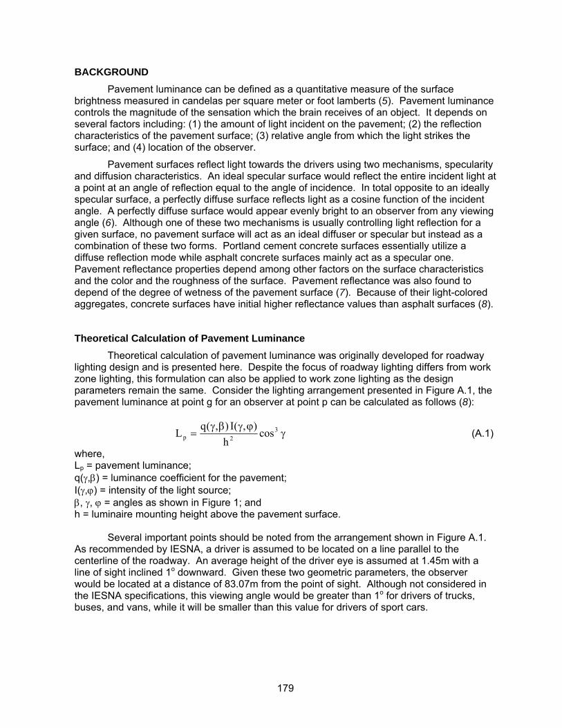
179
BACKGROUND Pavement luminance can be defined as a quantitative measure of the surface brightness measured in candelas per square meter or foot lamberts (5). Pavement luminance controls the magnitude of the sensation which the brain receives of an object. It depends on several factors including: (1) the amount of light incident on the pavement; (2) the reflection characteristics of the pavement surface; (3) relative angle from which the light strikes the surface; and (4) location of the observer.
Pavement surfaces reflect light towards the drivers using two mechanisms, specularity and diffusion characteristics. An ideal specular surface would reflect the entire incident light at a point at an angle of reflection equal to the angle of incidence. In total opposite to an ideally specular surface, a perfectly diffuse surface reflects light as a cosine function of the incident angle. A perfectly diffuse surface would appear evenly bright to an observer from any viewing angle (6). Although one of these two mechanisms is usually controlling light reflection for a given surface, no pavement surface will act as an ideal diffuser or specular but instead as a combination of these two forms. Portland cement concrete surfaces essentially utilize a diffuse reflection mode while asphalt concrete surfaces mainly act as a specular one. Pavement reflectance properties depend among other factors on the surface characteristics and the color and the roughness of the surface. Pavement reflectance was also found to depend of the degree of wetness of the pavement surface (7). Because of their light-colored aggregates, concrete surfaces have initial higher reflectance values than asphalt surfaces (8).
Theoretical Calculation of Pavement Luminance Theoretical calculation of pavement luminance was originally developed for roadway lighting design and is presented here. Despite the focus of roadway lighting differs from work zone lighting, this formulation can also be applied to work zone lighting as the design parameters remain the same. Consider the lighting arrangement presented in Figure A.1, the pavement luminance at point g for an observer at point p can be calculated as follows (8):
γϕγβγ
= 32p cos
h),(I),(qL (A.1)
where, Lp = pavement luminance; q(γ,β) = luminance coefficient for the pavement; I(γ,ϕ) = intensity of the light source; β, γ, ϕ = angles as shown in Figure 1; and h = luminaire mounting height above the pavement surface. Several important points should be noted from the arrangement shown in Figure A.1. As recommended by IESNA, a driver is assumed to be located on a line parallel to the centerline of the roadway. An average height of the driver eye is assumed at 1.45m with a line of sight inclined 1o downward. Given these two geometric parameters, the observer would be located at a distance of 83.07m from the point of sight. Although not considered in the IESNA specifications, this viewing angle would be greater than 1o for drivers of trucks, buses, and vans, while it will be smaller than this value for drivers of sport cars.

180
Figure A.1 Schematic Representation for Pavement Reflectance Calculations To simplify Equation (A.1), a reduced luminance coefficient is introduced such that: γβγ=βγ 3cos),(q),(r (A.2) From Equation (A.2) into Equation (1), we get:
2p hIrL = (A.3)
As noted from Equation (A.2), r is a function of γ and β. This parameter is usually arranged in two-dimensional arrays, called an r-Table. To account for the light loss factor, Equation (A.4) can be rewritten as:
2p hxMFLLFxIrL = (A.4)
where, LLF = light loss factor (a factor to consider illuminance depreciation with time under given operating conditions - assumed in this analysis 0.85); and MF = multiplication factor used by the r-table (usually 10,000). R-values have been estimated for major pavement surfaces and have been tabulated in what is referred to as r-tables. As an illustrative example, Table A.1(a) illustrates the r-values for a typical asphalt pavement surface as a function of γ and β. In general, pavement surfaces are classified into four major categories each with a specific set of r-values (i.e., R1 to R4). Table A.1(b) provides a general description of the different pavement categories (4). To determine pavement luminance using Equation (A.3), one can rely on the r-tables rather than directly measuring pavement luminance. Measurement of pavement reflectance requires the availability of a luminance meter, which is an expensive piece of equipment. Hence, to avoid
1.45m
g
β
γ
φ
83.07m
α = 1o
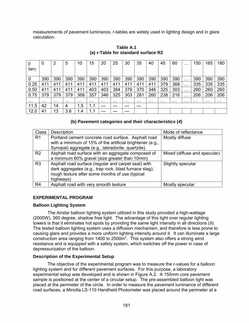
181
measurements of pavement luminance, r-tables are widely used in lighting design and in glare calculation.
Table A.1 (a) r-Table for standard surface R2
β tanγ
0 2 5 10 15 20 25 30 35 40 45 60 … 150 165 180
0 390 390 390 390 390 390 390 390 390 390 390 390 … 390 390 3900.25 411 411 411 411 411 411 411 411 411 411 379 368 … 335 335 3350.50 411 411 411 411 403 403 384 379 370 346 325 303 … 260 260 2600.75 379 379 379 368 357 346 325 303 281 260 238 216 … 206 206 206… … … … … … … … … … … … … … … … … 11.5 42 14 4 1.5 1.1 --- --- --- --- 12.0 41 13 3.6 1.4 1.1 --- --- ---
(b) Pavement categories and their characteristics (4)
Class Description Mode of reflectance R1 Portland cement concrete road surface. Asphalt road
with a minimum of 15% of the artificial brightener (e.g., Synopal) aggregate (e.g., labradorite, quartzite).
Mostly diffuse
R2 Asphalt road surface with an aggregate composed of a minimum 60% gravel (size greater than 10mm)
Mixed (diffuse and specular)
R3 Asphalt road surface (regular and carpet seal) with dark aggregates (e.g., trap rock, blast furnace slag); rough texture after some months of use (typical highways)
Slightly specular
R4 Asphalt road with very smooth texture Mostly specular
EXPERIMENTAL PROGRAM Balloon Lighting System The Airstar balloon lighting system utilized in this study provided a high-wattage (2000W), 360 degree, shadow free light. The advantage of this light over regular lighting towers is that it eliminates hot spots by providing the same light intensity in all directions (9). The tested balloon lighting system uses a diffusion mechanism, and therefore is less prone to causing glare and provides a more uniform lighting intensity around it. It can illuminate a large construction area ranging from 1400 to 2500m2. This system also offers a strong wind resistance and is equipped with a safety system, which switches off the power in case of depressurization of the balloon.
Description of the Experimental Setup The objective of the experimental program was to measure the r-values for a balloon lighting system and for different pavement surfaces. For this purpose, a laboratory experimental setup was developed and is shown in Figure A.2. A 150mm core pavement sample is positioned at the center of a circular setup. The pre-assembled balloon light was placed at the perimeter of the circle. In order to measure the pavement luminance of different road surfaces, a Minolta LS-110 Handheld Photometer was placed around the perimeter at a
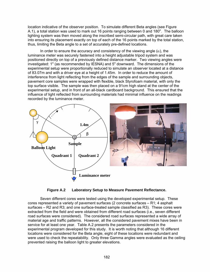
182
location indicative of the observer position. To simulate different Beta angles (see Figure A.1), a total station was used to mark out 16 points ranging between 0 and 180o. The balloon lighting system was then moved along the inscribed semi-circular path, with great care taken into ensuring its placement exactly on top of each of the 16 points marked by the total station, thus, limiting the Beta angle to a set of accurately pre-defined locations.
In order to ensure the accuracy and consistency of the viewing angle (α), the luminance meter was securely fastened into a height adjustable tripod system and was positioned directly on top of a previously defined distance marker. Two viewing angles were investigated: 1o (as recommended by IESNA) and 5o downward. The dimensions of the experimental setup were proportionally reduced to simulate an observer located at a distance of 83.07m and with a driver eye at a height of 1.45m. In order to reduce the amount of interference from light reflecting from the edges of the sample and surrounding objects, pavement core samples were wrapped with flexible, black Styrofoam material, with only the top surface visible. The sample was then placed on a 91cm high stand at the center of the experimental setup, and in front of an all-black cardboard background. This ensured that the influence of light reflected from surrounding materials had minimal influence on the readings recorded by the luminance meter.
Figure A.2 Laboratory Setup to Measure Pavement Reflectance.
Seven different cores were tested using the developed experimental setup. These cores represented a variety of pavement surfaces (2 concrete surfaces – R1; 4 asphalt surfaces – R2 and R3; and one surface-treated sample classified as R3). These cores were extracted from the field and were obtained from different road surfaces (i.e., seven different road surfaces were considered). The considered road surfaces represented a wide array of material age and traffic patterns. However, all the considered pavement mixes have been in service for at least one year. Table A.2 presents the parameters considered in the experimental program developed for this study. It is worth noting that although 16 different locations were considered for the Beta angle, eight of these locations were redundant and were used to check the repeatability. Only three Gamma angles were evaluated as the ceiling prevented raising the balloon light to greater elevations.
Balloon Light
1.4m
Luminance meter
β
γ
Sample
Quadrant 1 Quadrant 2

183
TABLE A.2 Parameters Considered in the Experimental Program
Factors Number of Levels Evaluated Levels
Road Surfaces 7 4 Asphalt Surfaces 2 Concrete Surfaces 1 Surface-Treated Surface
Beta Angle (β) 8^ From 90 to 180o
Viewing Angle (α) 2 1 and 5o downward
Gamma Angle (γ) 3 35, 40, 45o Lighting System 1 Balloon Lighting System ^: only eight different levels were evaluated. The other 8 levels were redundant and were used for check of repeatability.
Core ID C1 C2 C3 C4 C5 C6 C7
Description Concrete Asphalt Concrete Surface-Treated Asphalt Asphalt Asphalt
R-Class R1 R2 R1 R3 R3 R3 R2
RESULTS AND ANALYSIS Repeatability and General Trends of the Measurements As previously mentioned, measurements were conducted on both quadrants of the circular setup to evaluate their repeatability. This was accomplished by repetitively moving the balloon light on top of the predefined 16 locations. Figure 3 compares measurements obtained on both quadrants for the seven different cores. As shown in this figure, measurements were repeatable and consistent on both quadrants indicating the suitability of the experimental setup. Subsequent analysis was based on the average of the measurements in both quadrants.
Figure A.4 presents the variation of the R-values with different road surfaces and for different β angles (γ = 45o). As expected, the concrete surfaces (C1 and C3) had predominantly greater luminance values than the asphalt surfaces. However, one of the asphalt surfaces (C2) showed slightly greater pavement luminance than the concrete surfaces. Upon examination of this core, it was apparent that the aggregates in this surface were highly polished due to aging and traffic use, and, therefore, revealed a light-colored surface. Core C7, which was originally classified as an R2 surface type, also showed high luminance values comparable to the concrete cores. The rest of the asphalt cores (C4, C5, and C6) behaved as expected and provided pavement luminance values lower than the concrete surfaces. As previously mentioned, Portland cement concrete surfaces essentially utilize a diffuse reflection mode while asphalt surfaces mainly act as a specular one. Although concrete surfaces have an initial reflectance greater than asphalt surfaces, it is evident from this analysis that with aging and years of traffic, asphalt surfaces may exhibit a pavement luminance comparable to concrete surfaces.

184
0.0
2.0
4.0
6.0
8.0
10.0
12.0
14.0
16.0
18.0
0.0 2.0 4.0 6.0 8.0 10.0 12.0 14.0 16.0 18.0
Pavement Luminance - cd/m2 (First Quadrant)
Pave
men
t Lum
inan
ce -
cd/m
2 (Sec
ond
Qua
dran
t)
C1 C2C3 C4C5 C6C7
Figure A.3 Measured Pavement Luminance in the First and Second Quadrants (γ =
45o)
0
50
100
150
200
250
300
350
400
90 100 110 120 130 140 150 160 170 180
Beta Angle (o)
R-v
alue
s
C1 C2 C3 C4
C5 C6 C7
Figure A.4 Calculated R-Values for Different Road Surfaces (γ = 45o)

185
Effects of Viewing Angles Figure A.5 presents the effect of the viewing angles on the calculated r-values for selected cores. It was previously noted that IESNA assumes that a typical driver would look 1o downward towards the pavement. However, depending on the driver’s habits and the type of vehicles that he operates, this viewing angle may vary. As shown in Figure A.5, by looking downward with a viewing angle of 5o, pavement luminance substantially increases. As the amount of glare experienced by a driver would decrease with the increase in pavement luminance as he approaches a construction zone, it may be assumed that a viewing angle of 1o would be more critical to evaluate the worst-case scenario.
0
200
400
600
800
1000
1200
90 100 110 120 130 140 150 160 170 180
Beta Angle (o)
R-v
alue
s
C1 - 1degC1 - 5degC2 - 1degC2 - 5degC4 - 1degC4 - 5deg
Figure A.5 Variations of the R-Values with the Viewing Angles for Selected Cores
Comparison with R-tables Table A.3 compares the R-values obtained from the experimental program to the ones depicted by the R-tables as provided by IESNA. Values in bold are measured ones while values in black are the standard ones. Measured values were the average ones for the different cores according to the assigned R-Class. As it was previously mentioned, only three levels for the Gamma angle were investigated in this study due to ceiling limitations and elevation constraints of the balloon light system. However, since these three levels correspond to typical elevations for this lighting system, it is expected that these three levels simulated the predominant elevations encountered in field applications.
Upon evaluation of the data presented in Table A.3, one may note that the IESNA values only marginally changed with the increase in Beta angles. Moreover, the IESNA values appear to have contradicting trends depending on the road surfaces. While these values slightly increased with the increase in Beta angles for concrete surfaces, they kept constant or slightly decreased with the increase in Beta angles for asphalt surfaces. In contrast, measured values appear to gradually increase with the increase in Beta angles for
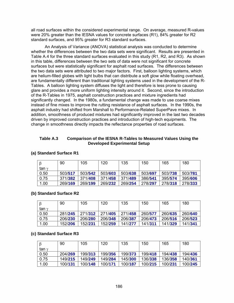
186
all road surfaces within the considered experimental range. On average, measured R-values were 20% greater than the IESNA values for concrete surfaces (R1), 84% greater for R2 standard surfaces, and 95% greater for R3 standard surfaces.
An Analysis of Variance (ANOVA) statistical analysis was conducted to determine whether the differences between the two data sets were significant. Results are presented in Table A.4 for the three standard surfaces evaluated in this study (R1, R2, and R3). As shown in this table, differences between the two sets of data were not significant for concrete surfaces but were statistically significant for asphalt road surfaces. The differences between the two data sets were attributed to two major factors. First, balloon lighting systems, which are helium-filled globes with light bulbs that can distribute a soft glow while floating overhead, are fundamentally different than traditional lighting systems used in the development of the R-Tables. A balloon lighting system diffuses the light and therefore is less prone to causing glare and provides a more uniform lighting intensity around it. Second, since the introduction of the R-Tables in 1975, asphalt construction practices and mixture ingredients had significantly changed. In the 1980s, a fundamental change was made to use coarse mixes instead of fine mixes to improve the rutting resistance of asphalt surfaces. In the 1990s, the asphalt industry had shifted from Marshall to Performance-Related SuperPave mixes. In addition, smoothness of produced mixtures had significantly improved in the last two decades driven by improved construction practices and introduction of high-tech equipments. The change in smoothness directly impacts the reflectance properties of road surfaces.
Table A.3 Comparison of the IESNA R-Tables to Measured Values Using the Developed Experimental Setup
(a) Standard Surface R1
β tan γ
90 105 120 135 150 165 180
0.50 503/517 503/542 503/603 503/638 503/697 503/738 503/781 0.75 371/382 371/408 371/458 371/489 386/541 395/574 395/606 1.00 269/169 269/199 269/232 269/254 278/297 278/318 278/333
(b) Standard Surface R2
β tan γ
90 105 120 135 150 165 180
0.50 281/245 271/312 271/405 271/458 260/577 260/635 260/640 0.75 206/230 206/280 206/348 206/387 206/473 206/516 206/523 1.00 152/206 152/231 152/259 141/277 141/311 141/329 141/341
(c) Standard Surface R3
β tan γ
90 105 120 135 150 165 180
0.50 204/269 199/313 199/356 199/373 199/418 194/438 194/436 0.75 149/215 149/249 149/284 145/300 136/338 136/358 140/361 1.00 100/131 100/148 100/171 100/187 100/215 100/231 100/245
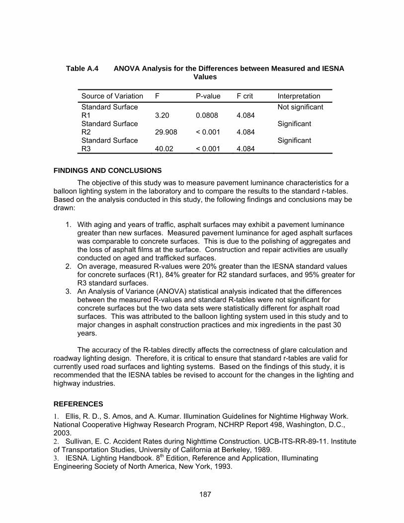
187
Table A.4 ANOVA Analysis for the Differences between Measured and IESNA Values
Source of Variation F P-value F crit Interpretation Standard Surface R1 3.20 0.0808 4.084
Not significant
Standard Surface R2 29.908 < 0.001 4.084
Significant
Standard Surface R3 40.02 < 0.001 4.084
Significant
FINDINGS AND CONCLUSIONS The objective of this study was to measure pavement luminance characteristics for a balloon lighting system in the laboratory and to compare the results to the standard r-tables. Based on the analysis conducted in this study, the following findings and conclusions may be drawn:
1. With aging and years of traffic, asphalt surfaces may exhibit a pavement luminance greater than new surfaces. Measured pavement luminance for aged asphalt surfaces was comparable to concrete surfaces. This is due to the polishing of aggregates and the loss of asphalt films at the surface. Construction and repair activities are usually conducted on aged and trafficked surfaces.
2. On average, measured R-values were 20% greater than the IESNA standard values for concrete surfaces (R1), 84% greater for R2 standard surfaces, and 95% greater for R3 standard surfaces.
3. An Analysis of Variance (ANOVA) statistical analysis indicated that the differences between the measured R-values and standard R-tables were not significant for concrete surfaces but the two data sets were statistically different for asphalt road surfaces. This was attributed to the balloon lighting system used in this study and to major changes in asphalt construction practices and mix ingredients in the past 30 years.
The accuracy of the R-tables directly affects the correctness of glare calculation and roadway lighting design. Therefore, it is critical to ensure that standard r-tables are valid for currently used road surfaces and lighting systems. Based on the findings of this study, it is recommended that the IESNA tables be revised to account for the changes in the lighting and highway industries.
REFERENCES 1. Ellis, R. D., S. Amos, and A. Kumar. Illumination Guidelines for Nightime Highway Work. National Cooperative Highway Research Program, NCHRP Report 498, Washington, D.C., 2003. 2. Sullivan, E. C. Accident Rates during Nighttime Construction. UCB-ITS-RR-89-11. Institute of Transportation Studies, University of California at Berkeley, 1989. 3. IESNA. Lighting Handbook. 8th Edition, Reference and Application, Illuminating Engineering Society of North America, New York, 1993.
188
4. IESNA. American National Standard Practice for Roadway Lighting. Report ANSI/IESNA RP-8-00, American National Standard/Illuminating Engineering Society of North America, USA, 2000. 5. Traister, J.E. Practical Lighting Application for Building Construction. Von Nost, 1982. 6. King, L.E. Measurement of Directional Reflectance of Pavement Surfaces and Development of Computer Techniques for Calculating Luminance. Journal of the Illuminating Engineering Society, Vol. 5, No. 2, 1976, pp. 118-126. 7. Bassett, M.G., D. Dmitrevsky, and P.C. Kremer. Measurement of Reflection Properties of Wet Pavement Samples. Journal of the Illuminating Engineering Society, Vol. 17, No. 2, 1988, pp. 99-104.
8. Khan, M.H., S. Senadheera, D.D. Gransberg, and R. Stemprock. Influence of Pavement Surface Characteristics on Nightime Visibility of Objects. Transportation Research Record 1692, TRB, Washington, D.C., 1999, pp. 39-48.
9. Airstar Space Lighting. Available at www.airstar-light.net, accessed 2007.