NICO DI MILAN ANO · I would also like to take this opportunity to thank Prof. Sergio Bittanti and...

APred

Superv

Analysdictive

visor: Prof

P

Scuol

Master o

sis ande Con

f. Riccardo

OLITEC

la di Inge

of Science

d Impntrol (M

o SCATTO

Academ

CNICO D

egneria de

e in Autom

lemenMPC)

OLINI

mic Year 201

DI MILAN

ell’Inform

mation E

ntation) in Ch

Ma

12/13

ANO

mazione

ngineerin

n of Mhemica

aster Gradu

Shahab Rez

Student Id.

ng

Model al Pla

uation Thesi

za BESHA

. number 76

nt

is by:

ARAT

64488

1

Abstract Model based Predictive Control (MPC) is a form of control that has gained widespread acceptance in chemical industry due to its unique advantages compared to classic control methods. The main distinguishing features are the ability to efficiently control large scale interconnected systems and the inherent ability to cope with physical and other constraints of the controlled system. MPC controllers are designed on the basis of a dynamical model of the system that has to be controlled (i.e., the plant) and apply mathematical optimization techniques in order to obtain the optimal inputs to be applied to the plant. MPC acquires the current control action by solving, at each sampling instant, a finite horizon open-loop optimal control problem, using the current state of the plant as the initial state; the optimization yields an optimal control sequence and the first control in this sequence is applied to the plant. In this thesis the focus is on linear MPC algorithms, i.e., MPC algorithms that can take the regulation problem. More specifically, the main aim of this thesis is the development of MPC algorithms in the environment of MATLAB and Simulink that can take input and output constraints into account and can guarantee stable behavior and acceptable performance. These aims are achieved by making improved algorithms for the construction of required matrixes and contributions to the constraints. On the level of stability, celebrated terminal state is enabled the pledge. We concentrate our attention on a plant with two reactors and a separator as a sample of chemical plant in order to enrich the experimental results. Several simulations on the model of this process show the improved properties of the obtained program. Keywords: Model predictive control; chemical plant; CSTR; optimal control; constraint; stability

2

Sommario Il controllo predittivo, o MPC (Model Predictive Control) è una tecnica di sintesi di sistemi di controllo che ha riscosso un notevole successo nell’industria chimica per I vantaggi che può offrire rispetto a metodi classici, quali l’assegnamento degli autovalori o il controllo LQR. Le sue principali caratteristiche sono la possibilità di considerare sistemi con grandi dimensioni, tipicamente costituiti da sottosistemi interconnessi, a la capacità di tenere conto in modo esplicito di eventuali vincoli sulle variabili di processo o su altre variabili di interesse. I controllori MPC sono di tipo “model-based”, cioè sono progettati a partire da un modello del processo sotto controllo, e si basano sulla formulazione di un opportuno problema di ottimizzazione da risolversi a ogni istante di campionamento per determinare il valore da imporre alle variabili di controllo. Più nello specifico, viene risolto un problema di controllo su orizzonte finito dove lo stato corrente è considerato come stato iniziale. La soluzione del problema di ottimo consiste nel determinare la sequenza di controlli ottimi da imporre, almeno teoricamente, lungo tutto l’intervallo considerato. Tuttavia, si implementa effettivamente soltanto il primo valore di questa sequenza e l’intera procedura è ripetuta al successivo istante di campionamento. In questo lavoro di Tesi si sviluppano in ambiente Matlab/Simulink due algoritmi MPC per sistemi lineari e se ne analizzano in dettaglio le caratteristiche e prestazioni. Entrambi gli algoritmi consentono di considerare vincoli sullo stato, sulle variabili di controllo e sulle uscite regolate, così da garantire stabilità e prestazioni. Per quanto riguarda la stabilità, è possibile introdurre nel problema di ottimizzazione un opportuno peso sullo stato finale raggiunto dal sistema al termine dell’orizzonte di predizione, vincolandolo anche ad appartenere a un dato insieme. Le caratteristiche di questi metodi MPC sono confrontate con riferimento a un processo, costituito da due reattori e da un separatore, in grado di rappresentare bene le problematiche tipiche di un impianto industriale. Nel lavoro sono riportate e commentate numerose simulazioni che consentono di mostrare le prestazioni ottenibili con questo approccio alla sintesi del controllore. Keywords: Model predictive control; chemical plant; CSTR; optimal control; constraint; stability

3

Acknowledgments

This thesis presents the results of the study carried out in the means of graduation on Master of Science in Automation engineering at Politecnico di Milano under the supervision of Prof. Riccardo Scattolini.

I would like to address a special word of gratitude to Prof. Scattolini; without whom the subject gathered in this thesis would have not been possible. Throughout my studies he took an active interest in my work and encouraged me to keep at it when I couldn’t see the light at the end of the tunnel. I will always be grateful for his investment of patience, time and effort in my work.

I would also like to take this opportunity to thank Prof. Sergio Bittanti and Prof. Paolo Rocco for allowing me to contribute in the IFAC Milano 2011 as a volunteer student. It was one of my greatest academicals experience.

A special thanks goes to Prof. Franco Zappa for his entire support to international students during the first days of university life in Milano and in the course “Electronic System”, at any time.

I am grateful to Prof. Marco Lovera and Prof. Alberto Leva for their astonishing classes in “Advanced and Multivariable Control” and “Automation of Energy systems” which were sources of inspiration for me.

During the two years I have studied on my Master program, I had the opportunity to spend enjoyable moments in the company of friends and colleagues. I would like to thank all of them.

I am eternally indebted to my wife Hananeh for her endless love and support and our parents for all their best wishes.

This thesis is dedicated to my wife.

Shahab R. Besharat Milano, December, 2012

4

ContentsAbstract .............................................................................................................................................. 1

Sommario ........................................................................................................................................... 2

Acknowledgments .............................................................................................................................. 3

List of Figures ..................................................................................................................................... 7

List of Tables ....................................................................................................................................... 9

Notation ........................................................................................................................................... 10

1 Introduction .................................................................................................................................. 12

1.1 Motivation .............................................................................................................................. 13

2 Dynamic model of chemical process ............................................................................................. 20

2.1 Introduction to process control ............................................................................................. 20

2.2 Process dynamic ..................................................................................................................... 20

2.3 Process control ....................................................................................................................... 21

2.4 The hierarchy of process control activities ............................................................................ 24

2.4.1 Measurement and actuation (Level 1) ............................................................................ 24

2.4.2 Safety and environmental/equipment protection (Level 2) ........................................... 25

2.4.3 Regulatory control (Level 3a) .......................................................................................... 25

2.4.4 Multivariable and constraint control (Level 3b) .............................................................. 25

2.4.5 Real‐time optimization (Level 4) ..................................................................................... 26

2.4.6 Planning and scheduling (Level 5) ................................................................................... 27

2.5 Continuous stirred tank reactor models ................................................................................ 29

2.5.1 The mass balance ............................................................................................................ 29

2.5.2 The component balance .................................................................................................. 30

2.5.3 Adding a chemical reaction to the stirred tank model ................................................... 31

2.5.4 The energy balance ......................................................................................................... 32

2.6 Case object ............................................................................................................................. 34

3 Model Predictive Control .............................................................................................................. 39

3.1 Historical issues on MPC in process control ........................................................................... 43

3.2 Open loop optimal control problem ...................................................................................... 46

5

3.3 Closed‐loop _ open‐loop analysis .......................................................................................... 50

3.3.1 IH‐LQ ................................................................................................................................ 50

3.3.2 FH optimal control .......................................................................................................... 51

3.3.3 RH problem ..................................................................................................................... 54

3.4 MPC formulation without integral action .............................................................................. 57

3.5 MPC formulation with integral action .................................................................................... 61

3.6 Extension to the basic formulation ........................................................................................ 65

4 Stability .......................................................................................................................................... 66

4.1 Stability analysis ..................................................................................................................... 66

4.1.1 Definitions ....................................................................................................................... 67

4.1.2 RH and IH‐LQ control....................................................................................................... 69

4.2 Stabilizing modifications ........................................................................................................ 71

4.2.1 Constrained IH‐LQ control ............................................................................................... 71

4.3 Achievements on MPC stability ............................................................................................. 75

5 Simulation in MATLAB and Simulink ............................................................................................. 76

5.1 Model of the system .............................................................................................................. 76

5.2 Linearization ........................................................................................................................... 76

5.3 Required matrix construction ................................................................................................ 81

5.4 Optimization by Quadprog ..................................................................................................... 83

5.4.1 Optimization for controller without Integral action ....................................................... 83

5.4.2 Optimization for controller with Integral action ............................................................. 84

5.5 Constraints ............................................................................................................................. 86

5.6 Controller design .................................................................................................................... 88

5.6.1 Controller without integral action .................................................................................. 88

5.6.2 Controller with integral action ........................................................................................ 90

6 Experimental results ..................................................................................................................... 92

6.1 Results for the MPC controller without integral action ......................................................... 93

6.1.1 Simulation 1: tuning the level of first reactor ................................................................. 93

6

6.1.2 Simulation 2: input weighting effect ............................................................................... 98

6.1.3 Simulation 3: output weighting effect .......................................................................... 100

6.1.4 Simulation 4: prediction and control horizons .............................................................. 102

6.1.5 Simulation 5: disturbance effect ................................................................................... 103

6.1.6 Simulation 6: input constraint ....................................................................................... 105

6.1.7 Simulation 7: output constraint .................................................................................... 106

6.1.8 Conclusion on MPC controller without integral action ................................................. 108

6.2 Results for MPC controller with integral action ................................................................... 109

6.2.1 Simulation 8: tuning the level of first reactor ............................................................... 109

6.2.2 Simulation 9: input weighting effect ............................................................................. 114

6.2.3 Simulation 10: output weighting effect ........................................................................ 116

6.2.4 Simulation 11: prediction and control horizons ............................................................ 117

6.2.5 Simulation 12: disturbance effect ................................................................................. 119

6.2.6 Simulation 13: input constraint ..................................................................................... 120

6.2.7 Simulation 14: output constraint .................................................................................. 121

6.2.8 Conclusion on MPC controller with integral action ...................................................... 123

Appendix A ..................................................................................................................................... 125

A.1 MATLAB codes of first subsystem model ............................................................................ 125

A.2 MATLAB codes for preparation of MPC parameters without integral action ..................... 126

A.3 MATLAB codes for construction of matrixes without integral action ................................. 126

A.4 MATLAB codes for MPC function without integral action ................................................... 129

A.5 MATLAB codes for preparation of MPC parameters with integral action ........................... 129

A.6 MATLAB codes for construction of matrixes with integral action ....................................... 130

A.7 MATLAB codes for MPC function with integral action ........................................................ 132

Bibliography ................................................................................................................................... 133

7

ListofFiguresFigure 1: Participants of APC survey by industry and by continent ................................................. 17

Figure 2: Industrial use of APC methods .......................................................................................... 17

Figure 3: Hierarchy of process control activities .............................................................................. 28

Figure 4: Mixed Tank of Liquid ......................................................................................................... 30

Figure 5: CSTR with cooling coil removing energy (Q) ..................................................................... 32

Figure 6: Two reactors in series with separator and recycle ........................................................... 35

Figure 7: Receding horizon scheme ................................................................................................. 54

Figure 8‐1: Plugging the integral action ........................................................................................... 63

Figure 8‐2: disappearing the integrator in augmented state block diagram ................................... 63

Figure 9: Integral action in augmented state block diagram ........................................................... 64

Figure 10: stabilized sets in the RH and IH‐LQ unconstrained control ............................................ 70

Figure 11: Stabilized sets in the constrained IH‐LQ control ............................................................. 73

Figure 12: Simulate the model with MATLAB function .................................................................... 78

Figure 13: the Model of fist reactor ................................................................................................. 78

Figure 14: intermediate scheme for first reactor model ................................................................. 79

Figure 15: Control diagram of MPC without integral action ............................................................ 88

Figure 16: MPC controller without integral action in Simulink ........................................................ 89

Figure 17: Control diagram of MPC with integral action ................................................................. 90

Figure 18: MPC controller with integral action in Simulink ............................................................. 91

Figure 19: Result of H1 setpoint change in the system.................................................................... 94

Figure 20: Result of H1 setpoint change in the system‐zoomed ..................................................... 95

Figure 21: Response of H1 to the setpont change ........................................................................... 96

Figure 22: Result of H1 setpoint change in Ff1, Ff2, H1 and H2 (normalized) ................................. 97

Figure 23: Result of input weighting with H1 setpoint change in Ff1, Ff2, H1 and H2 (normalized)99

Figure 24: Result of output weighting with H1 setpoint change in Ff1, Ff2, H1 and H2 (normalized)

........................................................................................................................................................ 101

Figure 25: Result of horizons with H1 setpoint change in Ff1, Ff2, H1 and H2 (normalized) ........ 103

Figure 26: Result of disturbance in the system .............................................................................. 104

Figure 27: Result of constraint for Ff1 with H1 setpoint change ................................................... 106

Figure 28: Result of constraint for T1 with H1 setpoint change .................................................... 107

Figure 29: Result of H1 setpoint change in the system with integrator ........................................ 110

Figure 30: Result of H1 setpoint change in the system with integrator‐zoomed .......................... 111

Figure 31: Response of H1 to the setpoint change with integrator ............................................... 112

Figure 32: Result of H1 setpoint change in Ff1, Ff2, H1 and H2 (normalized) with integrator ...... 113

Figure 33: Result of input weighting with H1 setpoint change in Ff1, Ff2, H1 and H2 (normalized)

with integrator ............................................................................................................................... 115

8

Figure 34: Result of output weighting with H1 setpoint change in Ff1, Ff2, H1 and H2 (normalized)

with integrator ............................................................................................................................... 117

Figure 35: Result of horizons with H1 setpoint change in Ff1, Ff2, H1 and H2 (normalized) with

integrator ....................................................................................................................................... 118

Figure 36: Result of disturbance in the system with integrator .................................................... 119

Figure 37: Result of constraint for dFf1 with H1 setpoint change with integrator ........................ 121

Figure 38: Result of constraint for H2 with H1 setpoint change with integrator .......................... 122

9

ListofTablesTable 1: Summary of linear MPC applications by areas ................................................................... 14

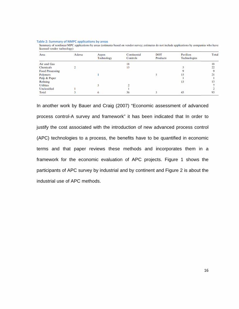
Table 2: Summary of NMPC applications by areas .......................................................................... 16

Table 3: Steady state and parameters ............................................................................................. 37

Table 4: Simulation1 parameters ..................................................................................................... 93

Table 5: Simulation2 parameters ..................................................................................................... 98

Table 6: Simulation3 parameters ................................................................................................... 100




Table 10: Simulation8 parameters ................................................................................................. 110

Table 11: Simulation9 parameters ................................................................................................. 114

Table 12: Simulation10 parameters ............................................................................................... 116




10

Notation

a, b, c ∈ Lower case roman symbols denote scalar or vector variables

A, B, C ∈ Upper case roman symbols denote matrix variables

, ∈ Upper case Unicode extended characters denote augmented

matrices

, Set of real numbers and positive real numbers

≔ Assignment

a ≔ b ⇔ the value of b is assigned to variable a

, (Strict) scalar inequality

a > b ⇔ a − b has strictly positive elements

, (Strict) matrix inequality

A > 0 ⇔ A is strictly positive definite

∈ m-dimensional input vector at discrete time k

∈ n-dimensional state vector at discrete time k

∈ p-dimensional output vector at discrete time k

∈ d-dimensional disturbance vector at discrete time k

, , Steady state values for inputs, states and outputs

Reference values for outputs or setpoint

Prediction horizon length

Control horizon length

, Transpose of matrix A

‖ ‖ Weighted 2-norm of a vector: ′

Function minimization over x,

optimal function value is returned

11

Motto:

“There is nothing more practical than a good theory.”

-Boltzmann

12

1Introduction

In this age of globalization, the realization of production innovation and highly

stable operation is the chief objective of the process industry. Obviously, modern

advanced control plays an important role to achieve this target, but the key to

success is the maximum utilization of PID control and conventional advanced

control. It is obvious that the three central pillars of process control – PID control,

conventional advanced control, and linear/nonlinear model predictive control –

have been widely used and they have to be contributed toward increasing

productivity.

Model predictive control (MPC) or receding horizon control (RHC) is a form of

control in which the current control action is obtained by solving on-line, at each

sampling instant, a finite horizon open-loop optimal control problem, using the

current state of the plant as the initial state; the optimization yields an optimal

control sequence and the first control in this sequence is applied to the plant. This

is its main difference from conventional control which uses a pre-computed control

law.

Model predictive control is one of few suitable methods, and this fact makes it an

important tool for the control engineer, particularly in the process industries where

plants being controlled are sufficiently slow to permit its implementation. Other

examples where model predictive control may be advantageously employed

13

include unconstrained nonlinear plants, for which on-line computation of a control

law usually requires the plant dynamics to possess a special structure, and time-

varying plants.

1.1Motivation

This thesis aims to reveal the principal of model predictive control, its formulation,

historical issues and some practical tricks. Finally, by implementing this theory in a

typical chemical process, as a plant consisting of two reactors and a separator in

the Simulink environment, try to represent the advantages of this state of the art

method. To motivate the idea of using MPC control, here are some fact according

to the international surveys and researches.

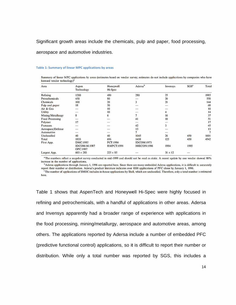
The first fact is coming from the article “A survey of industrial model predictive

control technology” by Quin and Badgwell (2003). According to their research, in

Tables 1 and 2, where more than 4600 total MPC applications are reported, MPC

technology can now be found in a wide variety of application areas. The largest

single block of applications is in refining, which amounts to 67% of all classified

applications. This is also one of the original application areas where MPC

technology has a solid track record of success. A significant number of

applications can also be found in petrochemicals and chemicals, although it has

taken longer for MPC technology to break into these areas.

Sign

aero

Table

Tab

refin

and

the

othe

(pre

distr

nificant grow

ospace and

1: Summary of

le 1 shows

ning and pe

Invensys a

food proce

ers. The ap

edictive func

ribution. W

wth areas

d automotive

linear MPC app

s that Aspe

etrochemica

apparently

essing, mini

pplications r

ctional cont

While only a

include the

e industries

plications by are

enTech an

als, with a

had a bro

ing/metallu

reported by

trol) applica

a total num

e chemicals

s.

as

d Honeywe

handful of

ader range

rgy, aerosp

y Adersa in

ations, so it

mber was

s, pulp and

ell Hi-Spec

application

e of experie

pace and a

nclude a nu

t is difficult

reported b

paper, foo

c were high

ns in other

ence with a

automotive

umber of em

to report th

by SGS, th

od process

hly focused

areas. Ade

applications

areas, amo

mbedded P

heir numbe

his includes

14

ing,

d in

ersa

s in

ong

PFC

r or

s a

15

number of in-house SMOC (Shell multivariable optimizing controller) applications

by Shell, so the distribution is likely to be shifted towards refining and

petrochemical applications.

The bottom of Table 1 lists the largest linear MPC applications to date by each

vendor, in the form of (outputs)_(inputs). The numbers show a difference in

philosophy that is a matter of some controversy.

AspenTech prefers to solve a large control problem with a single controller

application whenever possible; they report an olefins application with 603 outputs

and 283 inputs. Other vendors prefer to break the problem up into meaningful sub-

processes.

The nonlinear MPC (NMPC) applications reported in Table 2 are spread more

evenly among a number of applications areas. Areas with the largest number of

reported NMPC applications include chemicals, polymers, and air and gas

processing. It has been observed that the size and scope of NMPC applications

are typically much smaller than that of linear MPC applications. This is likely due to

the computational complexity of NMPC algorithms.

Table

In a

proc

justi

(APC

term

fram

part

indu

2: Summary of

another wor

cess contro

fy the cost

C) technolo

ms and tha

mework for

icipants of

ustrial use o

NMPC applicati

rk by Baue

ol-A survey

t associated

ogies to a

at paper

the econo

APC surve

of APC met

ions by areas

r and Craig

y and frame

d with the

process, th

reviews th

omic evalu

ey by indust

hods.

g (2007) “E

ework” it h

introduction

he benefits

hese metho

uation of A

trial and by

Economic a

has been in

n of new a

have to be

ods and i

APC projec

y continent a

assessmen

ndicated th

dvanced p

e quantified

incorporate

cts. Figure

and Figure

nt of advanc

hat In order

rocess con

d in econo

es them in

1 shows

2 is about

16

ced

r to

ntrol

mic

n a

the

the

Fina

in th

cont

MPC

past

ally to conc

he Journal

trol in Japa

C, releases

t, because

Figure 1: P

lude about

of Proces

an” is going

s operators

the optim

Participants of A

Figure 2: Ind

this motiva

s Control a

to be refer

from most

al operatin

APC survey by in

ustrial use of AP

ation, recen

as “The sta

rred. It has

t of the adju

ng conditio

ndustry and by c

PC methods nt paper of

ate of the

s been note

ustment wo

n is autom

continent

Kanu and O

art in che

ed that imp

ork they ha

matically de

Ogawa (20

mical proc

lementation

ad to do in

etermined a

17

010)

ess

n of

the

and

18

maintained under disturbances. In addition, MPC makes it possible to maximize

production rate by making the most use of the capability of the process and to

minimize cost through energy conservation by moving the operating condition

toward the control limit. Both the energy conservation and the productive capacity

were improved by an average of 3 to 5% as the result of APC projects centered on

MPC at Mitsubishi Chemical Corporation (MCC).

At the end of that paper, the MPC application for energy conservation and

production maximization of the olefin unit at MCCMizushima plant is briefly

explained which is the largest MPC application in the world, consisting of 283

manipulated variables and 603 controlled variables. The subsequent two

commentaries are appreciated to declaim.

A skilled operator made the following comment on this MPC application: “We had

operated the Ethylene fractionator in constant pressure mode for more than 20

years. I was speechless with surprise that we had made an enormous loss for

many years, when I watched the MPC decreased the column pressure, improved

the distillation efficiency, and maximized the production rate.” Another process

control engineer said “I had misunderstood that setpoints were determined by

operation section and process control section took the responsibility only for

control. I realized MPC for the first time; it makes the most use of the capability of

19

equipments, determines setpoints for economical operation, and maintains both

controlled variables and manipulated variables close to the setpoints.”

20

2Dynamicmodelofchemicalprocess

2.1Introductiontoprocesscontrol

In recent years the performance requirements for process plants have become

increasingly difficult to satisfy. Stronger competition, tougher environmental and

safety regulations, and rapidly changing economic conditions have been key

factors in tightening product quality specifications. A further complication is that

modern plants have become more difficult to operate because of the trend toward

complex and highly integrated processes. For such plants, it is difficult to prevent

disturbances from propagating from one unit to other interconnected units.

In view of the increased emphasis placed on safe, efficient plant operation, it is

only natural that the subject of process control has become increasingly important

in recent years. Without computer-based process control systems it would be

impossible to operate modern plants safely and profitably while satisfying product

quality and environmental requirements. Thus, it is important for Automation

engineers to have an overview about the process control.

2.2Processdynamic

The term process dynamics refers to unsteady-state (or transient) process

behavior. By contrast, most of the engineering may emphasize steady-state and

equilibrium conditions in subjects as material and energy balances,

thermodynamics, and transport phenomena. But process dynamics are also very

21

important. Transient operation occurs during important situations such as start-ups

and shutdowns, unusual process disturbances, and planned transitions from one

product grade to another.

2.3Processcontrol

The primary objective of process control is to maintain a process at the desired

operating conditions, safely and efficiently, while satisfying environmental and

product quality requirements. The subject of process control is concerned with

how to achieve these goals. In large-scale, integrated processing plants such as

oil refineries or ethylene plants, thousands of process variables such as

compositions, temperatures, and pressures are measured and must be controlled.

Fortunately, large numbers of process variables (mainly flow rates) can usually be

manipulated for this purpose. Feedback control systems compare measurements

with their desired values and then adjust the manipulated variables accordingly.

The foundation of process control is process understanding. Thus, we continue

with a basic question-What is a process? For our purposes, a brief definition is

appropriate:

Process: The conversion of feed materials to products using chemical and

physical operations. In practice, the term process tends to be used for both the

processing operation and the processing equipment.

22

Note that this definition applies to three types of common processes: continuous,

batch, and semibatch.

Following, we consider representative of continuous processes which is a main

subject of this thesis. Here briefly summarize key control issues.

The process control problem has been characterized by identifying three important

types of process variables.

• Controlled variables (CVs): The process variables that are controlled. The

desired value of a controlled variable is referred to as its set point.

• Manipulated variables (MVs): The process-Variables that can be adjusted in

order to keep the controlled variables at or near their set points. Typically, the

manipulated variables are flow rates.

• Disturbance variables (DVs): Process variables that affect the controlled

variables but cannot be manipulated. Disturbances generally are related to

changes in the operating environment of the process, for example, its feed

conditions or ambient temperature. Some disturbance variables can be measured

on-line, but many cannot.

23

The specification of CVs, MVs, and DVs is a critical step in developing a control

system. The selections should be based on process knowledge, experience, and

control objectives.

24

2.4Thehierarchyofprocesscontrolactivities

As mentioned earlier, the chief objective of process control is to maintain a

process at the desired operating conditions, safely and efficiently, while satisfying

environmental and product quality requirements.

If we emphasized one process control activity and try to keeping controlled

variables at specified set points, there are other important activities, also that we

will now briefly describe.

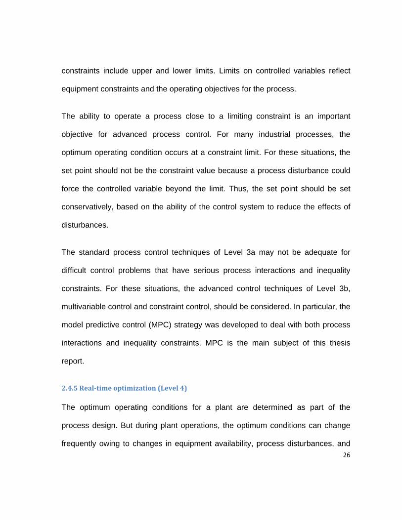
In Fig.3 the process control activities are organized in the form of a hierarchy with

required functions at the lower levels and desirable, but optional, functions at the

higher levels. The time scale for each activity is shown on the left side of Fig.3.

Note that the frequency of execution is much lower for the higher-level functions.

2.4.1Measurementandactuation(Level1)

Measurement devices (sensors and transmitters) and actuation equipment (for

example, control valves) are used to measure process variables and implement

the calculated control actions. These devices are interfaced to the control system.

Clearly, the measurement and actuation functions are an indispensable part of any

control system.

25

2.4.2Safetyandenvironmental/equipmentprotection(Level2)

The Level 2 functions play a critical role by ensuring that the process is operating

safely and satisfies environmental regulations. Generally, process safety relies on

the principle of multiple protection layers that involve groupings of equipment and

human actions. One layer includes process control functions, such as alarm

management during abnormal situations, and safety instrumented systems for

emergency shutdowns. The safety equipment operates independently of the

regular instrumentation used for regulatory control in Level 3a.

2.4.3Regulatorycontrol(Level3a)

As mentioned earlier, successful operation of a process requires that key process

variables such as flow rates, temperatures, pressures, and compositions be

operated at, or close to, their set points. This Level 3a activity, regulatory control,

is achieved by applying standard feedback and feedforward control techniques. If

the standard control techniques are not satisfactory, a variety of advanced control

techniques are available.

2.4.4Multivariableandconstraintcontrol(Level3b)

Many difficult process control problems have two distinguishing characteristics:

(i) significant interactions occur among key process variables, and (ii) inequality

constraints exist for manipulated and controlled variables. The inequality

26

constraints include upper and lower limits. Limits on controlled variables reflect

equipment constraints and the operating objectives for the process.

The ability to operate a process close to a limiting constraint is an important

objective for advanced process control. For many industrial processes, the

optimum operating condition occurs at a constraint limit. For these situations, the

set point should not be the constraint value because a process disturbance could

force the controlled variable beyond the limit. Thus, the set point should be set

conservatively, based on the ability of the control system to reduce the effects of

disturbances.

The standard process control techniques of Level 3a may not be adequate for

difficult control problems that have serious process interactions and inequality

constraints. For these situations, the advanced control techniques of Level 3b,

multivariable control and constraint control, should be considered. In particular, the

model predictive control (MPC) strategy was developed to deal with both process

interactions and inequality constraints. MPC is the main subject of this thesis

report.

2.4.5Real‐timeoptimization(Level4)

The optimum operating conditions for a plant are determined as part of the

process design. But during plant operations, the optimum conditions can change

frequently owing to changes in equipment availability, process disturbances, and

27

economic conditions. Consequently, it can be very profitable to recalculate the

optimum operating conditions on a regular basis. The new optimum conditions are

then implemented as set points for controlled variables.

The Level 4 activities also include data analysis to ensure that the process model

used in the RTO calculations is accurate for the current conditions.

2.4.6Planningandscheduling(Level5)

The highest level of the process control hierarchy is concerned with planning and

scheduling operations for the entire plant. For continuous processes, the

production rates of all products and intermediates must be planned and

coordinated based on equipment constraints, storage capacity, sales projections,

and the operation of other plants, sometimes on a global basis. Thus, planning

and scheduling activities pose difficult optimization problems that are based on

both engineering considerations and business projections.

28

`

Figure 3: Hierarchy of process control activities

< 1 second

< 1 second

seconds‐minuts

minutes‐hours

hours‐days

days‐months5. Planning and Scheduling

4. Real‐Time Optimization

3b. Multivariable and Constraint Control

3a. Regulatory Control

2. Safety and Environmental/

Equipment Protection

1. Measurement and Actuation

Process

29

2.5Continuousstirredtankreactormodels

Continuous stirred-tank reactors have widespread application in industry and

embody many features of other types of reactors. Chemical reactors are the most

influential and therefore important units that a chemical engineer will encounter. To

ensure the successful operation of a continuous stirred tank reactor (CSTR), it is

necessary to understand their dynamic characteristics. A good understanding will

ultimately enable effective control systems design. Consequently, a CSTR model

provides a convenient way of illustrating modeling principles for chemical reactors.

To describe the dynamic behavior of a CSTR, mass, component and energy

balance equations must be developed. This requires an understanding of the

functional expressions that describe chemical reaction. A reaction will create new

components while simultaneously reducing reactant concentrations. The reaction

may give off heat or my require energy to proceed. Hereafter the goal is a short

introduction of equations and modeling, while entire specification and

circumstances are available in any chemical dynamic references.

2.5.1Themassbalance

Rate of mass flow in – Rate of mass flow out = Rate of change of mass within

system

Con

dens

flow

Refe

For

the a

2.5.2

To

com

nsider a we

sity ρin. Th

w leaving the

erring to the

liquid syste

assumption

2Thecompo

develop a

mponents) w

ell-mixed ta

he volume o

e tank is F w

e mass bala

ems mass

n that liquid

onentbalan

a realistic

with respec

ank of liquid

of the liquid

with liquid d

Figure 4

ance,

balance eq

density is

nce

CSTR mo

ct to time m

d (Figure 4

d in the tan

density ρ.

4: Mixed Tank of

quation no

constant. A

odel, the

must be con

4). The inle

k is V, with

f Liquid

rmally can

Additionally

change of

nsidered. T

et stream flo

h constant d

be simplifi

as V = Ah

f individua

This is beca

ow is Fin w

density ρ. T

ied by mak

thus,

l species

ause individ

30

with

The

king

(or

dual

31

components can appear / disappear because of reaction (remember that the

overall mass of reactants and products will always stay the same). If there are N

components N – 1 component balances and an overall mass balance expression

are required. Alternatively a component balance may be written for each species.

A component balance for the jth chemical species is,

Rate of flow of jth component in – rate of flow of jth component out + rate of

formation of jth component from chemical reactions = rate of change of jth

component

2.5.3Addingachemicalreactiontothestirredtankmodel

Assume that the reaction may be described as, A → B, i.e. component A reacts

irreversibly to form component B. Further, assume that the reaction rate is 1st

order. Therefore the rate of reaction with respect to CA is modeled as,

The negative sign implies that CA disappears because of reaction. The component

balance differential equation is

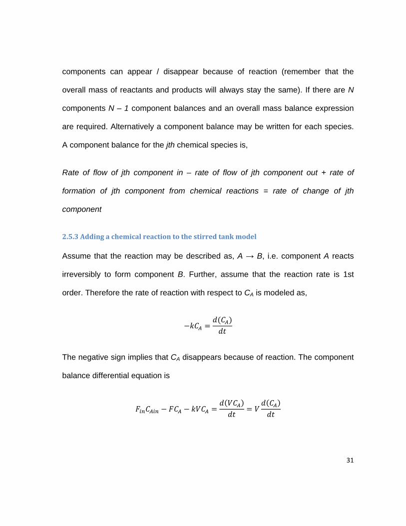
2.5.4

Rate

reac

The

rem

The

are

The

4Theenerg

e of energy

ction = rate

reaction (

ove any he

rate of he

assumed c

effect of te

ybalance

y flow in – r

of change

(A → B) is

eat generate

Figu

at removal

constant.

emperature

rate of ener

of energy w

s assumed

ed by react

ure 5: CSTR with

by the coo

on the rea

rgy flow ou

within syste

to be exo

tion.

h cooling coil rem

oling coil is

ction rate k

/

ut + rate at

em

othermic. A

moving energy (

s Q. Fluid s

k is usually

which heat

A cooling c

(Q)

specific hea

found to be

t added due

coil is used

at and den

e exponenti

32

e to

d to

sity

ial,

33

Where k0 is a pre-exponential (or Arrhenius) factor, E is the activation energy, T is

the reaction temperature and R is the gas law constant.

There are other considerations to complete the model of CSTR like, rate of heat

transfer through a cooling coil / jacket and dynamics of the reactor wall which have

been neglected for this short overview.

In summary, the dynamic model of the CSTR is nonlinear as a result of the many

product terms and the exponential temperature dependence of k in above

equation. Consequently, it must be solved by numerical integration techniques.

Additional species or chemical reactions may involve. If the reaction mechanism

involved production of an intermediate species, A → B → C, then unsteady-state

component balances for both A and B would be necessary, or balances for both A

and B could be written. Information concerning the reaction mechanisms would

also be required.

Reactions involving multiple species are described by high-order, highly coupled,

nonlinear reaction models because several component balances must be written.

Although the modeling task becomes much more complex, the same principles

illustrated above can be extended and applied.

34

2.6Caseobject

Real industrial chemical processes typically contain several reaction steps and

multiple recycle streams. Most process synthesis, controllability, and flexibility

studies in the literature have considered much simpler systems. In this report we

present a simplified version of a real complex industrial process. This example

illustrates many important characteristics of such systems like a complex flow

sheet, significant interactions among units with recycle streams, and numerous

byproduct / intermediate components. We think that this process would be utilized

by researchers in the areas of process synthesis and process control as a test

case for studying various techniques and approaches to problems in design and

control.

Refer to a rich plant modeling, taken from the article “Cooperative distributed

model predictive control” by Stewart, Venkat, Rawlings, Wright and Pannocchia

(2010); we consider in this thesis report, a plant consisting of two reactors and a

separator. A stream of pure reactant A is added to each reactor and converted to

the product B by a first-order reaction as illustrated in Figure 6. The product is lost

by a parallel first-order reaction to side product C. The distillate of the separator is

split and partially redirected to the first reactor.

The

model for t

1

1

1

1

1

Figure

the plant is

6: Two reactors

s in series with s

1

separator and re

ecycle

35

36

1

1

1 1

1

1

1

1

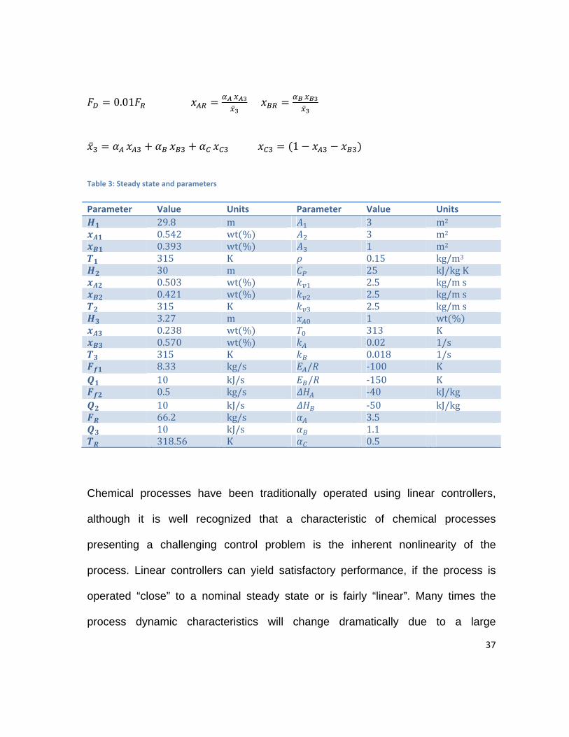
In which for all ∈ :

exp exp

The recycle flow and weight percents satisfy

37

0.01

1

Table 3: Steady state and parameters

Parameter Value Units Parameter Value Units

29.8 m 3 m2

0.542 wt % 3 m2 0.393 wt % 1 m2 315 K 0.15 kg/m3

30 m 25 kJ/kgK 0.503 wt % 2.5 kg/ms 0.421 wt % 2.5 kg/ms 315 K 2.5 kg/ms 3.27 m 1 wt % 0.238 wt % 313 K 0.570 wt % 0.02 1/s 315 K 0.018 1/s 8.33 kg/s / ‐100 K 10 kJ/s / ‐150 K 0.5 kg/s ‐40 kJ/kg 10 kJ/s ‐50 kJ/kg 66.2 kg/s 3.5 10 kJ/s 1.1 318.56 K 0.5

Chemical processes have been traditionally operated using linear controllers,

although it is well recognized that a characteristic of chemical processes

presenting a challenging control problem is the inherent nonlinearity of the

process. Linear controllers can yield satisfactory performance, if the process is

operated “close” to a nominal steady state or is fairly “linear”. Many times the

process dynamic characteristics will change dramatically due to a large

38

disturbance or due to significant setpoint changes from an on-line optimization

routine.

Consequently, chemical manufacturing processes present many challenging

control problems, including nonlinear dynamic behavior. Other common process

characteristics that cause control difficulty for linear and nonlinear systems alike

are:

multivariable interactions between manipulated and controlled variables

unmeasured state variables

unmeasured and frequent disturbances

high-order and distributed processes

uncertain and time-varying parameters

constraints on manipulated and state variables

deadtime on inputs and measurements

39

3ModelPredictiveControl

The only advanced control methodology which has made a significant impact on

industrial control engineering is predictive control. It has so far been applied mainly

in the petrochemical industry, but is currently being increasingly applied in other

sectors of the process industry. The main reasons for its success in these

applications are:

1. It handles multivariable control problems naturally.

2. It can take account of actuator limitations.

3. It allows operation closer to constraints (compared with conventional control),

which frequently leads to more profitable operation. Remarkably short pay-back

periods have been reported.

4. Control update rates are relatively low in these applications, so that there is

plenty of time for the necessary on-line computations.

In addition to the “constraint-aware optimizing” variety of predictive control, there is

an 'easy-to-tune, intuitive' variety, which puts less emphasis on constraints and

optimization, but more emphasis on simplicity and speed of computation, and is

particularly suitable for single-input, single-output (SISO) problems. This variety

has been applied in high-bandwidth applications such as servomechanisms, as

well as to relatively slow processes.

40

Model predictive control is an appropriately descriptive name for a class of model

based control schemes that utilize a process model for two central tasks (i) explicit

prediction of future process behavior, and (ii) computation of appropriate corrective

control action required to drive the predicted output as close as possible to the

desired target values. The overall objectives of an MPC may be summarized as:

• Prevent violations of input and output constraints.

• Drive some output variables to their optimal setpoints, while maintaining

other outputs within specified ranges.

• Prevent excessive movement of the input variables.

• Control as many process variables as possible when a sensor or actuator is

not available.

The ideas appearing to a greater or lesser degree, in all predictive controls are

basically:

• dependence of the control law on predicted behavior,

• explicit use of models to predict the process output at future time instants,

• calculation of control sequence minimizing an objective function, and

• receding horizon strategy, i.e., updating of input and shifting of the horizon

towards the future at each time instant.

41

Predictive control is intuitive and used in our daily activities like walking, driving,

studying and so on. Think about the course of studying in a school. Basically one

has to do a set of things:

• Predict: When one sets a target for a “desired” grade, one has to plan and work

towards the target. It may be too early to consider the final target at beginning of a

term. Instead, one should think a few days or a few weeks ahead and predict what

performance may be achieved over this shorter time window. The target within the

shorter time period can be, for example, certain “desired” grades in the

assignment, quiz, etc.

• Plan: Compare the predicted performance with the shorter time target. If a

difference is to be expected, for example, lower than the target, then additional

efforts should be considered, subject to constraints of course, such as there are

only 24 hours a day.

• Act: If it is expected that the additional efforts likely make one meet the target,

then the additional efforts will be put into action. Although a set of the additional

efforts, for today, tomorrow, and so on, has been planned days or weeks ahead,

only the effort planned for today can actually be materialized today. In the next

day, the procedure of prediction and planning is repeated, and a new set of efforts

is determined. Thus the next day’s action will be taken according to the new

planning. This process proceeds continuously until the end of the term.

42

Other well-known daily-life analogies in MPC literature include crossing a road and

playing chess. In chess, a good player predicts the game a few steps ahead based

on the moves of the opponent, and plans a few future moves. However, only one

move can actually be applied each time. Based on the following-up move of the

opponent, a new set of predictions has to be made and a new set of future moves

is determined as a result. This procedure is repeated throughout the game.

43

3.1HistoricalissuesonMPCinprocesscontrol

When MPC was first advocated by Richalet, Rault, Testud and Papon (1976) for

process control, several proposals for MPC had already been made, such as Lee

and Markus (1967), and, even earlier, a proposal, by Propoi (1963), of a form of

MPC, using linear programming, for linear systems with hard constraints on

control. However, the early proponents of MPC for process control proceeded

independently, addressing the needs and concerns of industry. Existing

techniques for control design, such as linear quadratic control, were not widely

used, perhaps because they were regarded as addressing inadequately the

problems raised by constraints, nonlinearities and uncertainty. The applications

envisaged were mainly in the petro-chemical and process industries, where

economic considerations required operating points (determined by solving linear

programs) situated on the boundary of the set of operating points satisfying all

constraints. The dynamic controller therefore has to cope adequately with

constraints that would otherwise be transgressed even with small disturbances.

The plants were modeled in the early literature by step or impulse responses.

These were easily understood by users and facilitated casting the optimal control

and identification problems in a form suitable for existing software.

Thus, IDCOM (identification and command), the form of MPC proposed in Richalet

et al. (1976,1978), employs a finite horizon pulse response (linear) model, a

quadratic cost function, and input and output constraints. The model permits linear

44

estimation, using least squares. The algorithm for solving the open-loop optimal

control problem is a “dual” of the estimation algorithm. As in dynamic matrix

control (DMC; Cutler & Ramaker, 1980; Prett & Gillette, 1980), which employs a

step response model but is, in other respects, similar, the treatment of control and

output constraints is ad hoc. This limitation was overcome in the second-

generation program, quadratic dynamic matrix control (QDMC; Garcia & Morshedi,

1986) where quadratic programming is employed to solve exactly the constrained

open-loop optimal control problem that results when the system is linear, the cost

quadratic, and the control and state constraints are defined by linear inequalities.

QDMC also permits, if required, temporary violation of some output constraints,

effectively enlarging the set of states that can be satisfactorily controlled. The third

generation of MPC technology, introduced about a decade ago, distinguishes

between several levels of constraints (hard, soft, ranked), provides some

mechanism to recover from an infeasible solution, addresses the issues resulting

from a control structure that changes in real time, and allows for a wider range of

process dynamics and controller specifications (Qin & Badgwell, 1997). In

particular, the Shell multivariable optimizing control (SMOC) algorithm allows for

state-space models, general disturbance models and state estimation via Kalman

filtering (Marquis & Broustail, 1988). The history of the three generations of MPC

technology, and the subsequent evolution of commercial MPC, is well described in

the last reference. The substantial impact that this technology has had on industry

45

is confirmed by the number of applications (probably exceeding 2000) that make it

a multi-million dollar industry.

The industrial proponents of MPC did not address stability theoretically, but were

obviously aware of its importance; their versions of MPC are not automatically

stabilizing. However, by restricting attention to stable plants, and choosing a

horizon large compared with the “settling” time of the plant, stability properties

associated with an infinite horizon are achieved. Academic research, stimulated by

the unparalleled success of MPC, commenced a theoretical investigation of

stability. Because Lyapunov techniques were not employed initially, stability had to

be addressed within the restrictive framework of linear analysis, confining attention

to model predictive control of linear unconstrained systems. The original finite

horizon formulation of the optimal control problem (without any modification to

ensure stability) was employed. Researchers therefore studied the effect of control

and cost horizons and cost parameters on stability when the system is linear, the

cost is quadratic, and hard constraints are absent. A typical result establishes the

existence of finite control and cost horizons such that the resultant model

predictive controller is stabilizing.

46

3.2Openloopoptimalcontrolproblem

The system to be controlled is usually described, or approximated, by an ordinary

differential equation, but since the control is normally piecewise constant, is

usually modeled, in the MPC literature, by a difference equation.

Consider the system

1 , ,

where ∈ and ∈ are the state and input vector, respectively. We

assume that the origin is an equilibrium point (f(0, 0) = 0).

We presumed the system to be specified in discrete time. One reason is that we

are looking for solutions to engineering problems. In practice, the controller will

always be implemented through a digital computer by sampling the variables of

the system and transmitting the control action to the system at discrete time

points. Another reason is that for the solution of the optimal control problems for

discrete-time systems, we will be able to make ready use of powerful

mathematical programming software. However, in many instances the discrete

time model is an approximation of the continuous time model.

According to the optimal control theory, the problem is to minimize the

performance index J (performance objective or cost function).

47

, , ,

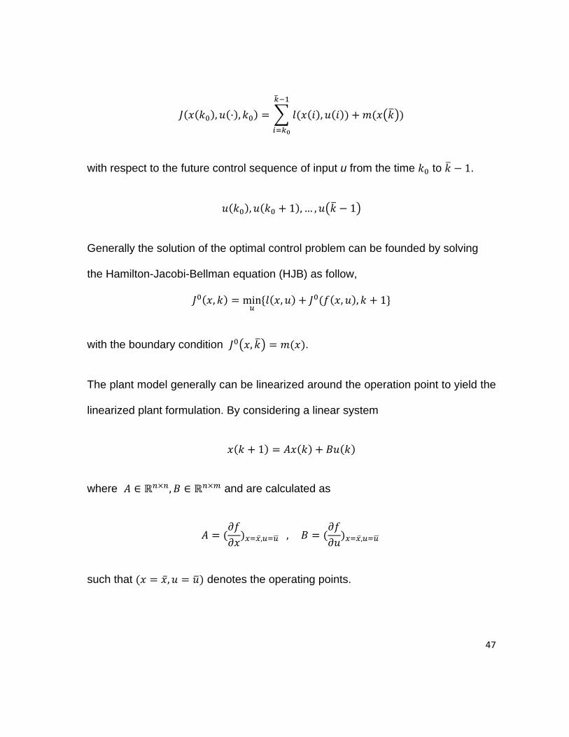
with respect to the future control sequence of input u from the time to 1.

, 1 , … , 1

Generally the solution of the optimal control problem can be founded by solving

the Hamilton-Jacobi-Bellman equation (HJB) as follow,

, min , , , 1

with the boundary condition , .

The plant model generally can be linearized around the operation point to yield the

linearized plant formulation. By considering a linear system

1

where ∈ , ∈ and are calculated as

, , ,

such that , denotes the operating points.

48

Before introducing the quadratic cost function, it is restored to express some

definitions. Expressions like and , where x, u are vectors, Q and R are

symmetric matrices and indicate the transpose of vector x, are called

quadratic forms, and are often written as ‖ ‖ and ‖ ‖ respectively. They are

just compact representations of certain quadratic functions in several variables.

Considering a linear system and a quadratic cost function

, , 0, 0

, 0

where Q and S are state weighting or penalty and R is input weighting.

The problem is turned into Linear Quadratic Control (LQ), where the HJB

approach reduced to , with .

The solution is Finite Horizon (FH) problem and completely defined by the control

law

1 ′ ′ 1 ′

where ′ 1 ′ 1 1 ′ 1

with its boundary condition .

49

Meant for continuous processes which are operating over a long time period, it

would be interesting to solve the infinite horizon problem.

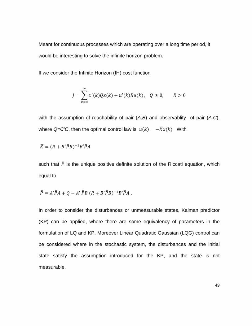
If we consider the Infinite Horizon (IH) cost function

, 0, 0

with the assumption of reachability of pair (A,B) and observablity of pair (A,C),

where Q=C’C, then the optimal control law is With

′

such that is the unique positive definite solution of the Riccati equation, which

equal to

′ ′ .

In order to consider the disturbances or unmeasurable states, Kalman predictor

(KP) can be applied, where there are some equivalency of parameters in the

formulation of LQ and KP. Moreover Linear Quadratic Gaussian (LQG) control can

be considered where in the stochastic system, the disturbances and the initial

state satisfy the assumption introduced for the KP, and the state is not

measurable.

50

3.3Closed‐loop_open‐loopanalysis

Through considering the system as 1 ∈ , ∈

and modifying the performance index as

, , ‖ ‖ ‖ ‖ ‖ ‖

Where 0, 0, 0 and outlining N as the so-called

prediction horizon, the stated problem is formed to minimizing the above

performance index J. Here we divide the general problem in three categories, and

try to formulate the problem with some consideration on the stability:

1- IH-LQ:

2- FH optimal control

3- Receding Horizon (RH)

3.3.1IH‐LQ

According to the previous result by the infinite horizon cost function and with the

assumption of reachability and observability, the optimal control law is

where K is calculated as ′

51

such that is obtained by finding the P as the unique positive definite solution of the

algebraic Riccati equation (ARE).

′ ′

Confined by these conditions for noted control law, the closed-loop system is

asymptotically stable.

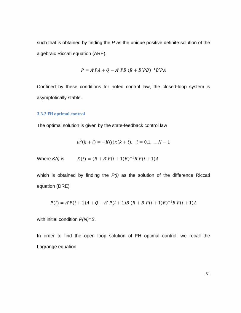
3.3.2FHoptimalcontrol

The optimal solution is given by the state-feedback control law

, 0,1, … , 1

Where K(i) is 1 ′ 1

which is obtained by finding the P(i) as the solution of the difference Riccati

equation (DRE)

1 ′ 1 1 ′ 1

with initial condition P(N)=S.

In order to find the open loop solution of FH optimal control, we recall the

Lagrange equation

52

, 0

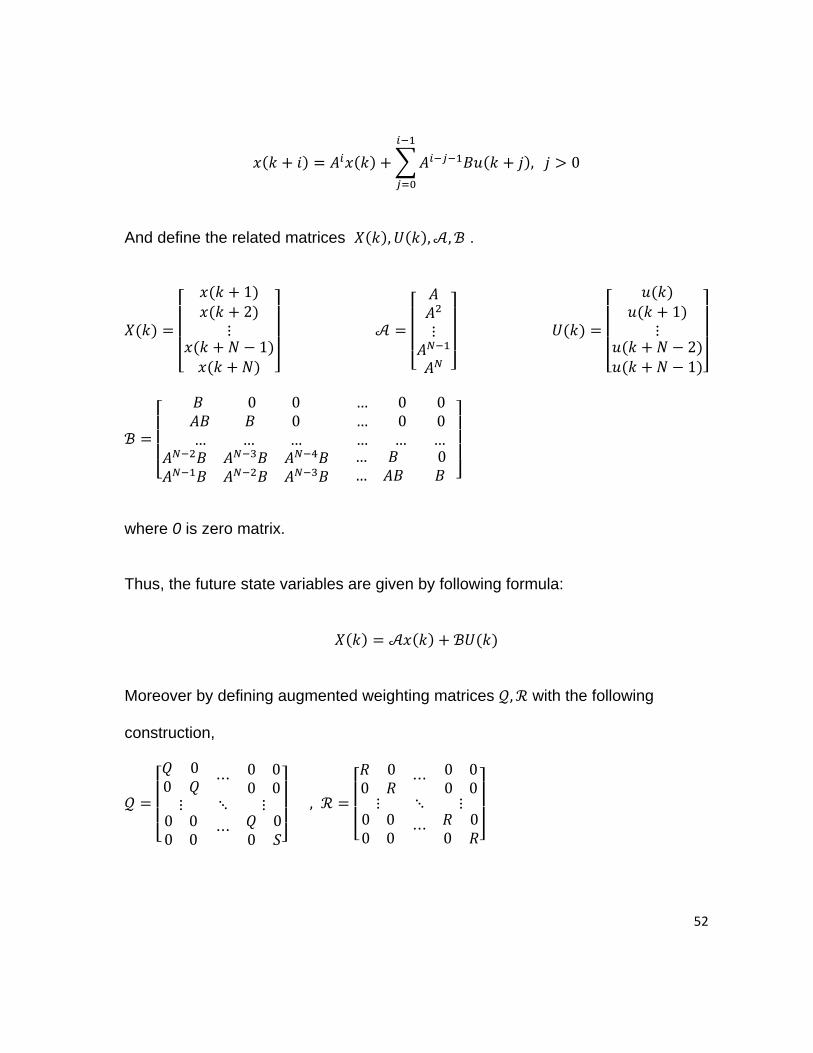
And define the related matrices , , , .

12

⋮1

⋮ 1

⋮21

0 0 0

… … …

… 0 0… 0 0… … …

… 0…

where 0 is zero matrix.

Thus, the future state variables are given by following formula:

Moreover by defining augmented weighting matrices , with the following

construction,

00 ⋯ 0 0

0 0⋮ ⋱ ⋮

0 00 0

⋯ 00

,

00

⋯ 0 00 0

⋮ ⋱ ⋮0 00 0

⋯ 00

53

and minimizing the modified performance index with respect to U(k), the open

loop solution is as follow:

, 0,1, … , 1

where depends on matrices , , and is calculated as follows.

The new modified performance index is

, , ′

where with respect to the original cost function, the terms has been

ignored, since it does not depend on U(k). By minimizing this new performance

index which can be rewrite in the form of quadratic function of U(k), its minimum

turns out to be ′ .

Thus, by letting ′ , is obtainable.

Note1: in the nominal case, the closed-loop and the open-loop solutions coincide.

Note2: if there are constraints on the control and/or state variables, the closed-

loop solution is not available, while the open-loop one can be reformulated as a

mathematical programming problem and can be easily solved by means of a QP

(quadratic programming) method with reduced computational time.

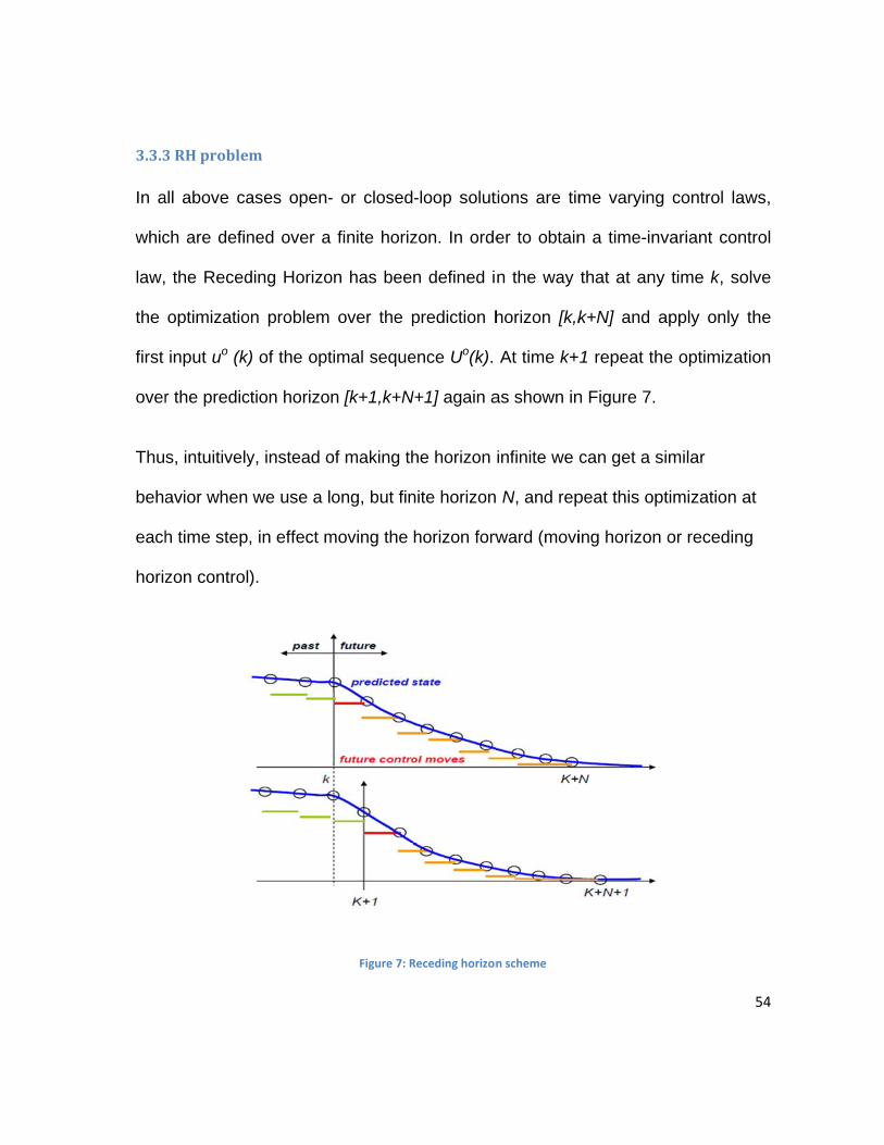
3.3.3

In a

whic

law,

the

first

over

Thu

beha

each

horiz

3RHproble

all above ca

ch are defin

the Reced

optimizatio

input uo (k)

r the predic

s, intuitively

avior when

h time step

zon control

m

ases open-

ned over a

ding Horizo

on problem

k) of the opt

ction horizo

y, instead o

we use a l

, in effect m

).

- or closed

finite horiz

on has bee

over the p

timal seque

n [k+1,k+N

of making th

ong, but fin

moving the

Figure 7: R

-loop solut

zon. In orde

n defined i

prediction h

ence Uo(k).

N+1] again a

he horizon

nite horizon

horizon forw

Receding horizon

tions are tim

er to obtain

n the way

horizon [k,k

At time k+

as shown in

infinite we

N, and rep

ward (movi

n scheme

me varying

n a time-inv

that at any

k+N] and a

1 repeat th

n Figure 7.

can get a s

peat this op

ing horizon

g control la

variant con

y time k, so

apply only

he optimizat

similar

ptimization a

or recedin

54

aws,

ntrol

olve

the

tion

at

g

55

The RH principle allows one to obtain the state-feedback time-invariant control

law.

ĸ

Intended for constrained systems, this control law is implicitly defined, while in the

unconstrained case, it coincides with the first element of the open-loop solution

and the first element of the closed-loop solution obtained by iterating the Riccati

equation backwards from P(N)=S.

First element of the open-loop solution is:

0

First element of the closed-loop solution is:

0 , 0 1 ′ 1

Thus the receding horizon solution formed as

0 0

Noted that, it is not a-priori guaranteed that the RH control law stabilizes the

closed-loop. In some cases, stability may be achieved only with the large

prediction horizon.

From this point upward, the formulation of the MPC can be modified according to

the applications, nevertheless the principle of receding horizon endure intrinsic in

56

all of these formulations. As a matter of fact that the subject of this report is

setpoint tracking or in general terms, regulation problem to control some

parameters within operation region in the chemical processes, the effect of

introducing reference signals and disturbances with their considerations, are going

to be discussed here after.

57

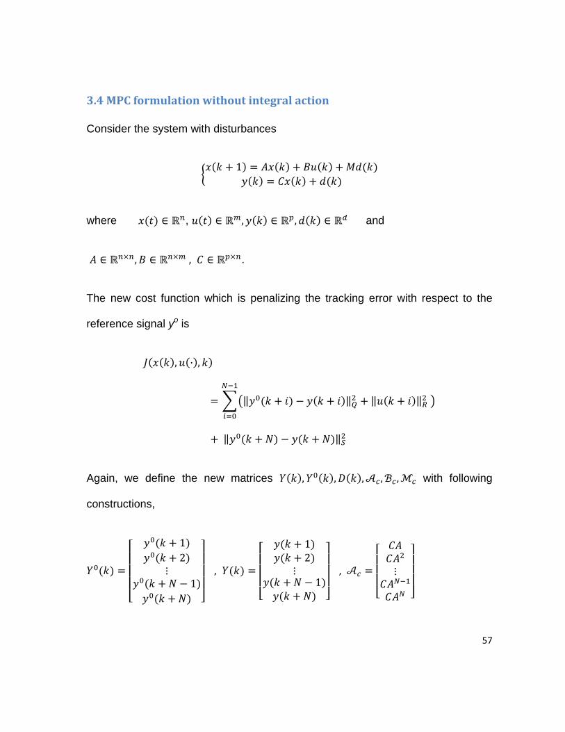
3.4MPCformulationwithoutintegralaction

Consider the system with disturbances

1

where ∈ , ∈ , ∈ , ∈ and

∈ , ∈ , ∈ .

The new cost function which is penalizing the tracking error with respect to the

reference signal yo is

, ,

‖ ‖ ‖ ‖

‖ ‖

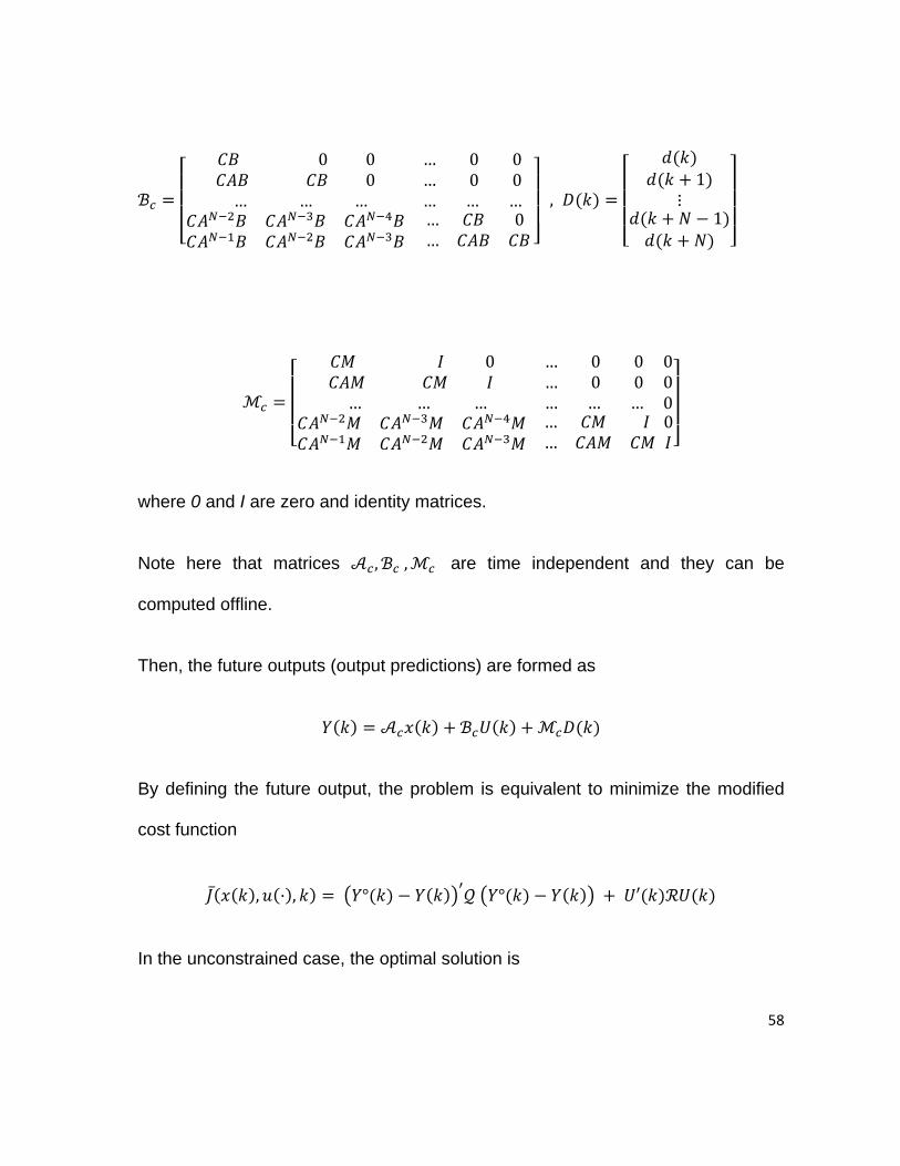
Again, we define the new matrices , , , , , with following

constructions,

12

⋮1

,

12

⋮1

, ⋮

58

0 0 0

… … …

… 0 0… 0 0… … …

… 0…

,1

⋮1

0

… … …

… 0 0… 0 0… … …

000

……

0

where 0 and I are zero and identity matrices.

Note here that matrices , , are time independent and they can be

computed offline.

Then, the future outputs (output predictions) are formed as

By defining the future output, the problem is equivalent to minimize the modified

cost function

, , ° ° ′

In the unconstrained case, the optimal solution is

59

°

which depends on the future reference signals Yo(k) and on the future

disturbances D(k). The optimal solution arise the motivation to state that, the

model predictive control can “anticipate” future reference variations or the effect of

known disturbances.

Note1: there is not any integral action which has been forced in the feedback

control law, therefore with assumption of providing the closed-loop stability, for

constant reference signal, steady state zero error regulation cannot be achieved.

Note2: In all above considered cases, the state x(k) has been assumed to be

measurable. Otherwise an observer can be utilized. Likewise to estimate the

disturbance d(k) when it is unmeasurable.

Note3: When the future disturbance is unknown, it is a common practice to set

, 0 .

In the case of control regulation with the constant reference signals y0, by

assuming that there exists a pair , such that

a more significant performance index has been fashioned as follow:

60

, , ‖ ‖ ‖ ‖ ‖ ‖

This performance index penalizes the control deviation with respect to the desired

equilibrium point.

Note 4: this performance index does not penalize the state, subsequently in this

case proper observability or detectability assumption is advisable.

3.5

As t

zero

algo

the

As u

inpu

than

algo

conv

and

the d

The

the

rega

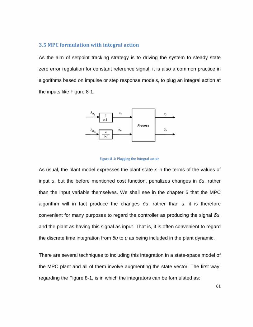
MPCform

the aim of

o error regu

orithms bas

inputs like F

usual, the p

ut u. but th

n the input

orithm will

venient for

the plant a

discrete tim

re are seve

MPC plant

arding the F

mulationw

setpoint tr

ulation for c

ed on impu

Figure 8-1.

plant model

e before m

variable th

in fact pro

many purp

as having th

me integratio

eral techniq

and all of

Figure 8-1,

withintegra

racking stra

constant ref

ulse or step

Figure 8‐1: P

l expresses

mentioned c

hemselves.

oduce the

poses to reg

his signal as

on from δu

ques to inclu

them involv

is in which

alaction

ategy is to

ference sig

p response

Plugging the inte

s the plant

cost functio

We shall s

changes

gard the co

s input. Tha

to u as bei

uding this in

ve augmen

the integra

driving the

gnal, it is al

models, to

egral action

state x in th

on, penalize

see in the

δu, rather

ontroller as

at is, it is of

ng included

ntegration i

nting the sta

ators can be

e system to

so a comm

plug an int

he terms of

es changes

chapter 5

r than u. i

producing

ften conven

d in the pla

in a state-s

ate vector.

e formulate

o steady st

mon practice

tegral action

f the values

s in δu, rat

that the M

it is theref

the signal

nient to reg

nt dynamic

pace mode

The first w

d as:

61

tate

e in

n at

s of

ther

MPC

fore

δu,

gard

c.

el of

way,

62

1

So the state-space form of the system plus integrators and by neglecting the

disturbances is obtained:

11 0

0

While the Performance index with tracking error and control variation is

, ,

‖ ‖ ‖ ‖

‖ ‖

In unconstrained case, the RH control law is linear as follow

But in the block diagram view of this system, the integrator disappears due to the

feedback term on signal v, as illustrated in Figure 8-2.

This

aga

s problem c

in the enlar

1

Figure 8‐2: dis

can be avoid

rged system

1

appearing the in

ded with an

m:

1

1 →

1

11

11

ntegrator in aug

n alternative

1

→ 1

1

0

gmented state b

e formulatio

1

block diagram

on of MPC

1 →

1

and exploit

1

63

ting

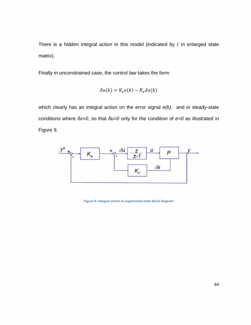
The

mat

Fina

whic

cond

Figu

re is a hid

rix).

ally in uncon

ch clearly h

ditions whe

ure 9.

den integra

nstrained c

has an inte

ere δx=0, s

Figure

al action in

ase, the co

gral action

o that δu=0

9: Integral actio

n this mode

ontrol law ta

on the err

0 only for t

on in augmented

el (indicate

akes the for

ror signal e

he conditio

d state block dia

ed by in e

rm

e(k), and in

on of e=0 a

agram

enlarged st

n steady-st

as illustrated

64

tate

tate

d in

65

3.6Extensiontothebasicformulation

The main MPC algorithms are characterized by a number of “tricks” which make

them very different from a classical LQ algorithm. Some of these tricks are Control

horizon, Minimum prediction horizon, Reference filtering, Filtering of disturbances

and High level optimization. Among them, we just take a short view on control

horizon which will be used in the generation of MPC algorithm of chemical plants.

If the prediction horizon N is sufficiently large, the number of optimization variables

(or the future control increments) can make the optimization problem difficult to

solve. For this reason, and to obtain a slower control action, it is often assumed

that the control variables remain constant after Nu<N time instants.

1 , , … , 1

or

0, , … , 1

In this case, the cost function can be written as follow

, ,

‖ ‖ ‖ ‖

‖ ‖

which is going to be used widely, by the advantages of easier optimization

problem.

66

4Stability

Early versions of MPC and generalized predictive control did not automatically

ensure stability, thus requiring tuning. It is therefore not surprising that research in

the 1990s devoted considerable attention to this topic. Indeed, concern for stability

has been a major engine for generating different formulations of MPC. In time,

differences between model predictive, generalized predictive, and receding

horizon control became irrelevant; we therefore use MPC as a generic title in the

consequence for that mode of control in which the current control action is

determined by solving on-line an optimal control problem.

4.1Stabilityanalysis

Model predictive control of constrained systems is nonlinear necessitating the use

of Lyapunov stability theory, that the value function (of a finite horizon optimal

control problem) could be used as Lyapunov function to establish stability of

receding horizon control of unconstrained systems when a terminal equality

constraint is employed. These results extended that the value function as a

Lyapunov function for establishing stability of model predictive control of time-

varying, constrained, nonlinear, discrete-time systems (when a terminal equality

constraint is employed); thereafter, the value function was almost universally

employed as a natural Lyapunov function for stability analysis of model predictive

control.

67

4.1.1Definitions

While asymptotic convergence of the state x(k) in the form of lim → x k → 0 is a

desirable property, it is generally not sufficient in practice. We would also like a

system to stay in a small neighborhood of the origin when it is disturbed by a little.

Formally this is expressed as Lyapunov stability.

Consider the system

1 , 0

Where is an arbitrary (discontinuous) function and is equilibrium point if

.

Letting ⊆ an open neighborhood of , then is stable, unstable, attractive,

asymptotically stable and exponentially stable according to the following

conditions:

Stable, if, for each 0, there is such that

‖ ‖ → ‖ ‖ for any 0.

Unstable, if not stable.

Attractive in if

68

lim → ‖ ‖ 0 for any ∈ .

Asymptotically stable in , if it is stable and attractive in .

Exponentially stable in , if there exist 0, ∈ 0,1 such that

‖ ‖ ‖ ‖ for any 0.

The ε, δ requirement for stability definition takes a challenge-answer form. To

demonstrate that the origin is stable, for any value of ε that a challenger may

chose (however small), we must produce a value of δ such that a trajectory

starting in a δ neighborhood of the origin will never leave the ε neighborhood of the

origin.

Function : → is a K function if it is continuous, strictly increasing with

0 0.

Usually to show Lyapunov stability of the origin for a particular system, one

constructs a so called Lyapunov function, i.e., a function satisfying the conditions

of the following theorem.

Let ⊆ be a positively invariant set for the system

1

69

containing a neighborhood of the equilibrium x 0 .

Undertake that , , be the class K functions and assume that there exist a

nonnegative scalar function : → , 0 0 such that

‖ ‖ ,∀ ∈

‖ ‖ ,∀ ∈

∆ ‖ ‖ ,∀ ∈

Then the origin is an asymptotically stable equilibrium in . Moreover, if

‖ ‖ ≔ ‖ ‖ , ‖ ‖ ≔ ‖ ‖ , ‖ ‖ ≔ ‖ ‖ for some , , , 0 and

, then the origin is exponentially stable in .

We use the extension of the Lyapunov theory by considering non continuous

Lyapunov functions (the cost function in constrained MPC control) and refer to

Figure10.

4.1.2RHandIH‐LQcontrol

Considering linear system with measurable state

1

and its performance index

, ∑ ‖ ‖ ‖ ‖ ‖ ‖ .

Acco

outli

Term

with

Main

Aux

horiz

By

func

gua

ording to R

ining in the

minal cost:

the choice

n control la

iliary contro

zon onward

considering

ction and w

rantees sta

RH and IH-L

following.

a cost pe

e wh

w: which is

ol law: whic

ds.

g these as

with a suit

ability in the

Figure 10: s

LQ control i

enalizing no

ich is ‖

s the RH so

ch is assum

ssumptions,

table choic

e unconstra

stabilized sets in

n unconstra

on zero sta

‖ .

lution

med to be u

, the resul

ce of the t

ined case.

n the RH and IH‐

ained case

ate at the e

used from

lting J is t

terminal co

‐LQ unconstrain

e, some term

end of pred

0 .

the end of

the classica

ost, the R

ned control

minologies

diction horiz

the predict

al IH-LQ c

H control

70

are

zon

tion

cost

law

71

4.2Stabilizingmodifications

There are many methods for modifying the open-loop optimal control problem ( )

employed in model predictive control of constrained systems so that closed-loop

stability could be guaranteed.

The modifications correspond, mainly for the terminal cost and the terminal

constraint set.

4.2.1ConstrainedIH‐LQcontrol

Considering the following IH constrained problem

min , ‖ ‖ ‖ ‖

∈ , 0

∈ , 0

where U and X are closed sets containing the origin, Q>0, R>0.

The solution of this problem cannot be computed with the HJB equation or with the

open-loop solution in view of the infinite number of constraints to be considered.

However the solution of the stated optimization problem can be found by solving,

with a sufficiently long prediction horizon N and with the RH strategy. Thus the FH

optimal control problem is

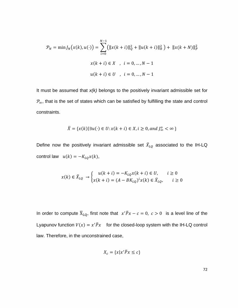
72

min , ‖ ‖ ‖ ‖ ‖ ‖

∈ , 0, … , 1

∈ , 0, … , 1

It must be assumed that x(k) belongs to the positively invariant admissible set for

, that is the set of states which can be satisfied by fulfilling the state and control

constraints.

|∃ ∈ : ∈ , 0, ∞

Define now the positively invariant admissible set associated to the IH-LQ

control law ,

∈ →∈ , 0

∈ , 0

In order to compute X , first note that 0, 0 is a level line of the

Lyapunov function for the closed-loop system with the IH-LQ control

law. Therefore, in the unconstrained case,

|

is a

ther

for a

illus

Fina

exis

of th

positively

re is a prosp

any c such

trated in F

ally it can b

sts a (comp

he associate

invariant se

pect to find

h that ⊆

igure 11.

Figure

be proven

putable) suf

ed problem

et for the c

a set

∈

⊆ , it grad

e 11: Stabilized s

that by let

fficiently lon

m is such

closed-loop

des that

sets in the const

tting ∈

ng predictio

h that

∈

system wi

∈

is the re

trained IH‐LQ co

∈ and by

on horizon

.

th IH-LQ c

quired set

ontrol

y given a s

N such tha

control. Now

X , which

set X , th

at the solut

73

w, if

h is

here

tion

74

The computation of an upper bound of N can be performed with results available

in the literature. Assuming that this value has been determined, in view of the

dynamic programming approach, the solution of coincides with the solution of

. In fact, the terminal cost of is the cost to go of the IH problem.

The discussion above reveals the presence of several ingredients that have been

found useful in developing stabilizing model predictive controllers; these

ingredients are a terminal cost, a terminal constraint set, and a local controller.

There are more conditions in the relevant literature on these ingredients, which if

satisfied, ensure that the model predictive controller is stabilizing.

75

4.3AchievementsonMPCstability

Research on stability of model predictive controlled systems has now reached a

relatively mature stage. The important factors for stability have been isolated and

employed to develop a range of model predictive controllers that are stabilizing

and differ only in their choice of the three ingredients (i) terminal cost, (ii) terminal

constraint set and (iii) local controller, that are common to most forms of model

predictive control. These conditions are merely sufficient and several researchers

are seeking relaxations.

76

5SimulationinMATLABandSimulink

5.1Modelofthesystem

According to the plant which consist of two reactors and a separator and their

models which are described in Chapter 2, the plant has been divided in three

subsystems and consequently three MATLAB functions have been constructed by

utilizing differential equation in mfiles, relatively. These files are available in

Appendix A.

5.2Linearization

The model of the system has been described regarding the dynamic previously

introduced, in differential equations. As it hold the nonlinear properties, first it must

be converted to the linear model (Linearization continues/discrete).

How to compute the linearized model? There are many ways to linearize a

nonlinear model and mostly work around the equilibrium point. One of the simplest

ways in the environment of Simulink is by using the block “Timed-Based

Linearization” which allows to numerically computing at the given time instant the

linearized model of an overall nonlinear system. This block calls “linmod” or

“dlinmod” to create a linear model for the system when the simulation clock

reaches the time specified by the Linearization time parameter. No trimming is

performed. The linear model is stored in the base workspace as a structure, along

77

with information about the operating point at which the snapshot was taken.

Multiple snapshots are appended to form an array of structures.

In order to use “Timed-Based Linearization” block, the open loop system must be

built, define the inputs and define the additional input port, which correspond to the

real input of linearized system. The same way to define the output of linearized

model with output ports must be applied. Then the system must be executed for

constant values. There have to be sure that at the time that Simulink wants to

compute the linearized model, the system must be in steady state. Simulink

automatically computes the linearized model, by giving small variation to each

input and looking at the result on each output (numerically linearization technique).

This approach is critical sometimes and need some precautions since for the

unstable system, it can be very dangerous. However for stable system, there is a

prior guarantee that after the linearization time, system remains in steady state

position, and the result is reliable.

There are ways to simulate the model, like S-function and etc., but there is a

simple way to use MATLAB functions in Simulink with a simple trick. This trick is

schemed in Figure 12.

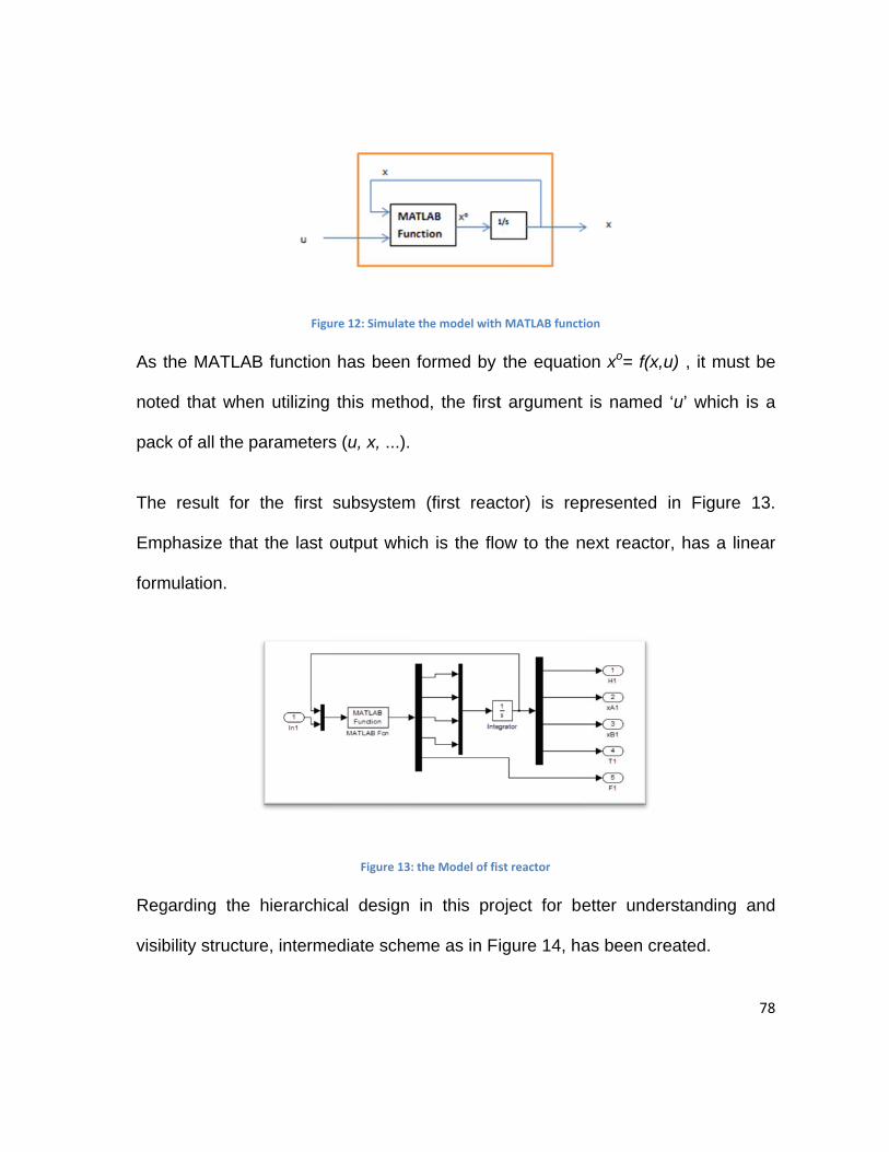
As t

note

pack

The

Emp

form

Reg

visib

the MATLA

ed that whe

k of all the

result for

phasize tha

mulation.

garding the

bility structu

Figu

AB function

en utilizing

parameters

r the first

at the last o

e hierarchic

ure, interme

ure 12: Simulate

has been

this metho

s (u, x, ...).

subsystem

output whic

Figure 13:

cal design

ediate sche

the model with

formed by

od, the first

(first reac

ch is the flo

the Model of fis

in this pro

me as in Fi

h MATLAB funct

the equatio

t argument

ctor) is rep

ow to the n

st reactor

oject for be

igure 14, ha

tion

on xo= f(x,u

t is named

presented

next reacto

etter unde

as been cre

u) , it must

‘u’ which i

in Figure

r, has a lin

rstanding a

eated.

78

t be

is a

13.

near

and

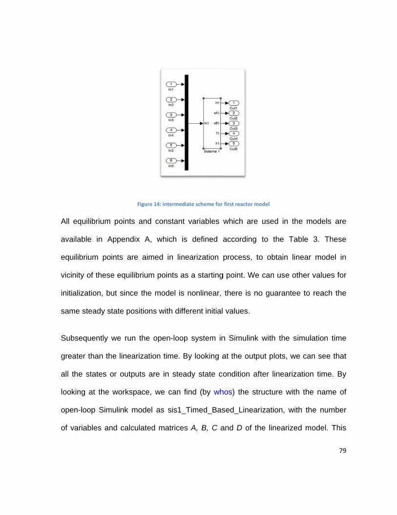
All e

avai

equ

vicin

initia

sam

Sub

grea

all t

look

ope

of v

equilibrium

ilable in A

ilibrium po

nity of these

alization, bu

me steady st

bsequently w

ater than th

he states o

king at the

n-loop Sim

ariables an

Figur

points and

Appendix A

ints are ai

e equilibriu

ut since the

tate positio

we run the

he linearizat

or outputs

workspace

mulink mode

nd calculate

re 14: intermedi

d constant

A, which is

med in line

m points as

e model is

ns with diff

e open-loop

tion time. B

are in stea

e, we can f

el as sis1_

ed matrices

iate scheme for

variables

s defined

earization

s a starting

nonlinear,

erent initial

p system in

By looking a

ady state co

find (by wh

_Timed_Bas

s A, B, C a

first reactor mo

which are

according

process, to

g point. We

there is no

values.

n Simulink

at the outp

ondition aft

hos) the str

sed_Linear

and D of th

odel

used in th

to the Ta

o obtain lin

can use ot

o guarantee

with the s

ut plots, we

fter lineariz

ructure with

rization, wit

he linearize

he models

able 3. The

near mode

ther values

e to reach

imulation t

e can see t

ation time.

h the name

th the num

ed model. T

79

are

ese

el in

s for

the

ime

that

By

e of

mber

This

80

method is surprisingly practical. By these matrices, the linearized model can be

prepared. Therefore once we yield the linearized model, by means of off-line

calculated matrices of the model, they can be exploited for controller design.

81

5.3Requiredmatrixconstruction

In order to use MPC formulation in MATLAB and in general framework, we need to

construct some matrices. With the reference to the Chapter 3, about the

formulation of MPC, the constructions of these matrices are coming in the

following.

As the result of linearization procedure is obtained in the continuous mode, first we

must convert the system matrices from continuous to discrete-time models with

specified sampling time in order to obtain (A, B, C) matrices in discrete mode. The

effect of disturbances can be introduced within construction of matrix M. by making

this M matrix equal to zero, can simply neglect the disturbances. In next step, by

using “DLQR” command in MATLAB, which is the Linear-quadratic (LQ) state-

feedback regulator for discrete-time state-space system, the optimal gain matrix K

can be calculated, such that the state-feedback law minimizes the quadratic cost

function. In addition to the state-feedback gain K, DLQR returns the infinite horizon

solution S of the associated discrete-time Riccati Equation and the closed-loop

eigenvalues.

Subsequently, by defining the weighting matrices, prediction horizon, control

horizon and finally constraint on inputs (manipulated variables) and outputs/states,

relative matrices have been formed. To insure the stability, terminal constraint has

been formed finally and been enforced to zero.

82

There is also one specific algorithm for reduced size of matrices in the case that

the control horizon is less than prediction horizon, which can reduce the

computations.

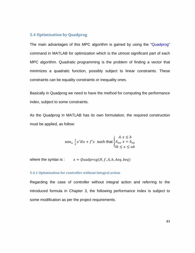
83

5.4OptimizationbyQuadprog

The main advantages of this MPC algorithm is gained by using the “Quadprog”

command in MATLAB for optimization which is the utmost significant part of each

MPC algorithm. Quadratic programming is the problem of finding a vector that

minimizes a quadratic function, possibly subject to linear constraints. These

constraints can be equality constraints or inequality ones.

Basically in Quadprog we need to have the method for computing the performance

index, subject to some constraints.

As the Quadprog in MATLAB has its own formulation, the required construction

must be applied, as follow:

min ′ such that ..

where the syntax is : , , , , ,

5.4.1OptimizationforcontrollerwithoutIntegralaction

Regarding the case of controller without integral action and referring to the

introduced formula in Chapter 3, the following performance index is subject to

some modification as per the project requirements.

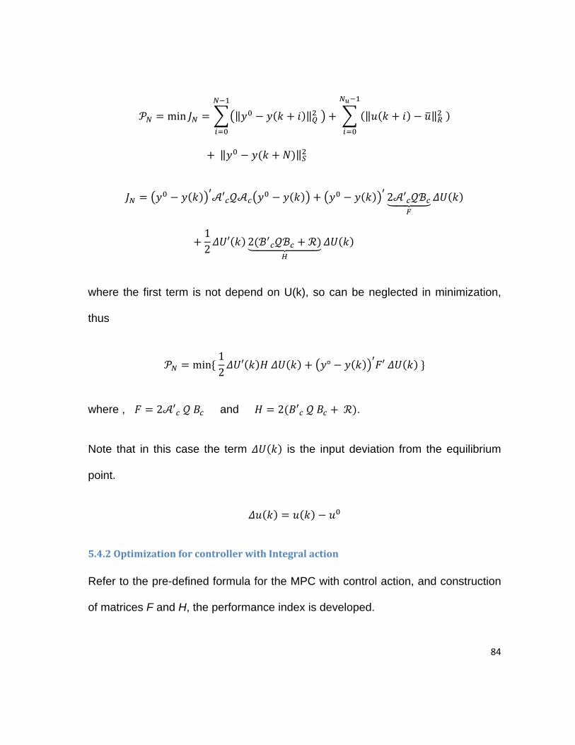
84

min ‖ ‖ ‖ ‖

‖ ‖

′ 2 ′

12

′ 2

where the first term is not depend on U(k), so can be neglected in minimization,

thus

min 12

′ ° ′

where , 2 ′ and 2 ′ .

Note that in this case the term is the input deviation from the equilibrium

point.

5.4.2OptimizationforcontrollerwithIntegralaction

Refer to the pre-defined formula for the MPC with control action, and construction

of matrices F and H, the performance index is developed.

85

min ‖ ‖ ‖ ‖ ‖ ‖

min 12

°

Note that in this case the term is the input increment.

1

86

5.5Constraints

MPC controller is nothing, but applying the first vector of Quadratic programming

optimization as a control variable to the plant. By contributing different constraint

for inputs, outputs and adding terminal constraint to this approach, different results

may arise due to the theory of MPC control which has been discussed in Chapters

3 and 4.

Nearly every application imposes constraints; actuators are naturally limited in the

force (or equivalent) they can apply, safety limits states such as temperature,

pressure and velocity and efficiency often dictates steady-state operation close to

the boundary of the set of permissible states. The prevalence of hard constraints is

accompanied by a lack of control methods for handling them, despite a continuous

demand from industry that has had, in their absence, to resort often to ad hoc

methods

The formulations for constraint cases are divided in two portions. Inequality

constraints are related to the saturation or high/low limits in input, or may some

technological limits or safety issues on output or state. Equality constraint is cause

of some guarantee for stability which may lead to computing terminal state or

terminal constraint, all according to the subject of optimization in quadratic

programming method. The general form of inequality constraint is:

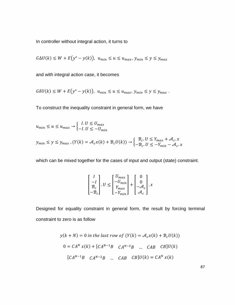
87

In controller without integral action, it turns to

∆ ° , ,

and with integral action case, it becomes

° , , .

To construct the inequality constraint in general form, we have

→..

, →. .. .

which can be mixed together for the cases of input and output (state) constraint.

.

00 .

Designed for equality constraint in general form, the result by forcing terminal

constraint to zero is as follow

0

0 …

…

5.6

5.6.1

Acco

outp

Due

rega

diag

The

in s

simu

Controller

1Controller

ording to th

put and inpu

e to the cen

arding the

gram is ach

MPC algor

tate-space

ulations.

rdesign

rwithoutint

he model of

ut are deno

ntralized str

general fo

ieved.

Figure

rithm has b

, in this wa

tegralaction

f the plant c

oted, respec

rategy of th

rmula for t

15: Control diag

been develo

ay we hav

n

consisting o

ctively:

e controller

the MPC i

gram of MPC wi

oped accord

e discrete-

of two reac

r and the a

n Chapter

ithout integral a

ding to the

-time contro

ctors and a

aim of the r

3, the fol

action

discrete-tim

oller and c

separator,

egulation, a

lowing con

me formulat

continues t

88

the

and

ntrol

tion

ime

In th

MPC

outp

we

man

by f

cont

illus

As i

stea

his controlle

C controller

puts are dev

need to

nipulated va

feedback to

troller will b

trates the im

it has been

ady state va

er, the state

r, inputs of

viation of c

accumulate

ariables to

o calculate

be discusse

mplementa

Figure 1

n presented

alues in the

es and outp

the MPC a

control varia

e them by

the proces

e the error

ed on the C

ation of this

16: MPC controll

d by the co

e control loo

puts are eq

are the err

ables from t

y their ste

ss. Controll

from the s

hapter 6 by

controller i

ler without inte

ontrol sche

op, while if

quivalent. D

ror on the s

their steady

eady state

ed values

setpoint. M

y some sim

n Simulink.

egral action in Si

eme, there

f the equilib

Due to the c

states or ou

y state valu

e values t

as output o

More specif

mulation res

.

imulink

is always a

brium point

construction

utputs, and

ues. Theref

to derive

or state ret

fication of

ults. Figure

a necessity

of the syst

89

n of

d its

fore

the

turn

this

e 16

y of

tem

chan

be m

Ano

cont

stea

cont

follo

5.6.2

Acco

tech

cons

form

nges due to

modified in

other drawb

troller struc

ady state e

troller in o

owing.

2Controller

ording to

hnique pro

struction o

mulation. Th

o the opera

the structur

back of this

cture, zero

error on th

order to inc

rwithintegr

the formul

mote by u

of the MP

he general

Figur

ation region

re, which m

s controller

steady sta

he outputs

clude the

ralaction

lation of M

using the

C controlle

scheme of

re 17: Control di

n of the pro

make a disa

is that sinc

ate could n

. This pro

integral ac

MPC with

enlarged s

er with in

this contro

iagram of MPC w

cess in the

advantages

ce there is

ot be guar

oblem moti

ction, whic

integral ac

system. Th

ntegral acti

oller represe

with integral act

e time, thes

for this con

no integra

ranteed and

vates us t

ch is the s

ction in C

his matter

ion with r

ented in Fig

tion

se values m

ntroller.

al action in

d may hav

to modify

subject of

hapter 3,

changed

respect to

g. 17.

90

must

the

ve a

the

the

the

the

its

The

of t

feed

abo

Figu

Acco

ther

actio

formulatio

his control

dback, and

ut this con

ure 18 illust

ording to th

re are som

on, where is

n employs

ller consist

the error

troller will

rates the im

Figure

he modifica

me adjustme

s indicated

the increm

t of deviat

on the ou

be discuss

mplementat

e 18: MPC contro

tions with r

ents in the

in Append

ment of con

tion of sta

tput of the

sed on Cha

tion of this c

oller with integr

respect to t

e constructi

ix A.

trol variabl

ates which

e system. M

apter 6 by

controller in

ral action in Sim

he controlle

ion of relat

e and state

come from

More detai

some simu

n Simulink.

mulink

er without i

ted matrice

es. The inp

m the filte

il specificat

ulation resu

ntegral act

es for integ

91

puts

ered

tion

ults.

ion,

gral

92

6Experimentalresults

In this thesis report, two methods for implementing the MPC controller are

discussed and related formula and considerations have been disposed. The first

approach is the controller without integral action and the second one is by

concerning the integral action. In order to assess the control performance and

stability issue of the model predictive controller structured in the previous chapters,

we perform the simulations and try to conclude with an overview of the different

controllers with enforcing assortments of parameters, compared here. To

recognize the advantages and disadvantages of each method, the plots of control

and state variables are depicted in this chapter.

As the problem arises in the multivariable space, the stream of graphs is settled to

illustrate the contribution of changed parameter in the entire system, or in some

case by associating two selected variables. In point of fact, in the methodology of

centralized controller, there is not any independent loop in the system and all the

loops are coupled. For this intention the construction of any decoupling and

modifying the problem to the different SISO cases like decentralized control

approach is intolerable. Contained by this tactic, better recognition of a plant as a

unique system has been achieved.

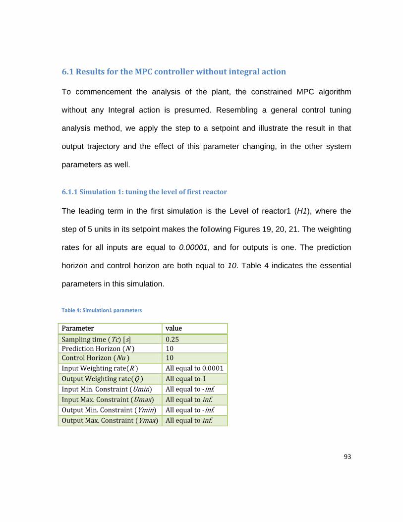
93

6.1ResultsfortheMPCcontrollerwithoutintegralaction

To commencement the analysis of the plant, the constrained MPC algorithm

without any Integral action is presumed. Resembling a general control tuning

analysis method, we apply the step to a setpoint and illustrate the result in that

output trajectory and the effect of this parameter changing, in the other system

parameters as well.

6.1.1Simulation1:tuningtheleveloffirstreactor

The leading term in the first simulation is the Level of reactor1 (H1), where the

step of 5 units in its setpoint makes the following Figures 19, 20, 21. The weighting

rates for all inputs are equal to 0.00001, and for outputs is one. The prediction

horizon and control horizon are both equal to 10. Table 4 indicates the essential

parameters in this simulation.

Table 4: Simulation1 parameters

Parameter value

Samplingtime Tc s 0.25PredictionHorizon N 10ControlHorizon Nu 10InputWeightingrate R Allequal to0.0001OutputWeightingrate Q Allequalto1InputMin.Constraint Umin Allequalto‐inf.InputMax.Constraint Umax Allequaltoinf.OutputMin.Constraint Ymin Allequalto‐inf.OutputMax.Constraint Ymax Allequaltoinf.

Figu

app

ure 19 illust

lied in the t

trate the tun

ime 100, th

Figu

ning on H1

he zoomed

ure 19: Result of

in the enti

plot has be

f H1 setpoint cha

re plant va

een shown

ange in the syst

ariables. Sin

in Figure 2

tem

nce the ste

0.

94

p is

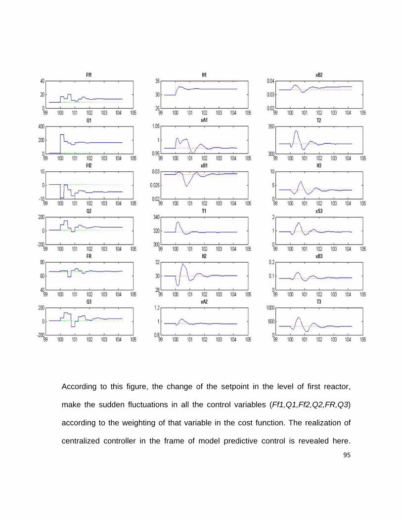
Acco

mak

acco

cent

ording to t

ke the sudd

ording to th

tralized con

his figure,

den fluctua

he weightin

ntroller in t

Figure 20:

the chang

ations in all

ng of that v

the frame

Result of H1 se

e of the se

l the contro

ariable in t

of model p

etpoint change in

etpoint in t

ol variables

the cost fun

predictive c

n the system‐zo

the level o

s (Ff1,Q1,F

nction. The

control is r

oomed

of first reac

Ff2,Q2,FR,Q

e realization

revealed he

95

ctor,

Q3)

n of

ere.

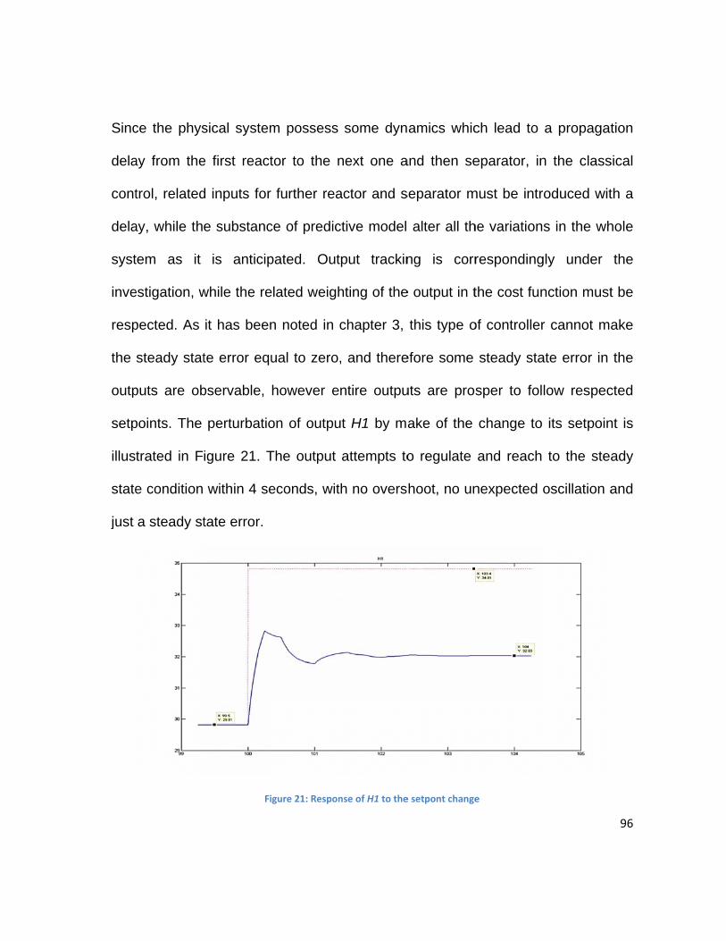
Sinc

dela

cont

dela

syst

inve

resp

the

outp

setp

illus

state

just

ce the phys

ay from the

trol, related

ay, while th

tem as it

estigation, w

pected. As

steady stat

puts are ob

points. The

trated in F

e condition

a steady st

sical system

e first react

d inputs for

e substanc

is anticip

while the re

it has been

te error equ

bservable,

perturbatio

igure 21. T

within 4 se

tate error.

Fi

m possess

tor to the n

further rea

ce of predic

pated. Out

elated weigh

n noted in

ual to zero

however e

on of outpu

The output

econds, wit

gure 21: Respon

some dyn

next one a

actor and s

ctive model

tput trackin

hting of the

chapter 3,

, and there

ntire outpu

ut H1 by m

attempts to

th no overs

nse of H1 to the

amics whic

and then se

separator m

alter all th

ng is corr

e output in t

this type o

efore some

uts are pros

ake of the

o regulate

hoot, no un

e setpont change

ch lead to

eparator, in

must be intr

he variation

responding

the cost fun

of controller

steady sta

sper to fol

change to

and reach

nexpected o

e

a propagat

n the class

roduced wit

s in the wh

gly under

nction must

r cannot ma

ate error in

low respec

its setpoin

to the stea

oscillation a

96

tion

sical

th a

hole

the

t be

ake

the

cted

nt is

ady

and

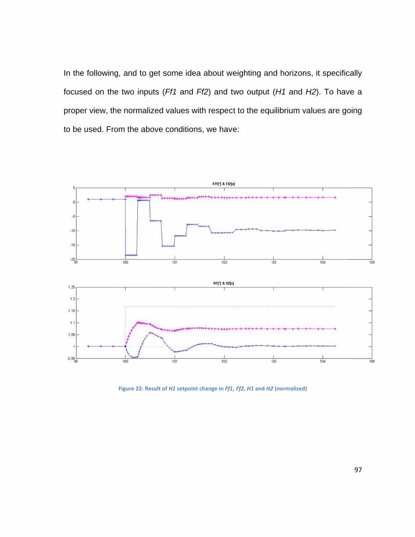
In th

focu

prop

to be

he following

used on the

per view, th

e used. Fro

g, and to ge

e two input

e normalize

om the abov

Figure 22: Resu

et some ide

s (Ff1 and

ed values w

ve condition

ult of H1 setpoin

ea about we

Ff2) and t

with respec

ns, we have

nt change in Ff1,

eighting an

two output

ct to the equ

e:

, Ff2, H1 and H2

nd horizons

(H1 and H

uilibrium va

2 (normalized)

s, it specific

H2). To hav

lues are go

97

cally

ve a

oing

98

6.1.2Simulation2:inputweightingeffect

Through increasing the weighting rate of the first input among the others by the

value of 1.1, and with respect to the parameters in Table 5, the following result has

been achieved in Figure 23.


Parameter value

Samplingtime Tc s 0.25PredictionHorizon N 10ControlHorizon Nu 10InputWeightingrate R R Ff1 equalto1.1

Therest equalto0.0001OutputWeightingrate Q Allequalto1InputMin.Constraint Umin Allequalto‐inf.InputMax.Constraint Umax Allequaltoinf.OutputMin.Constraint Ymin Allequalto‐inf.OutputMax.Constraint Ymax Allequaltoinf.

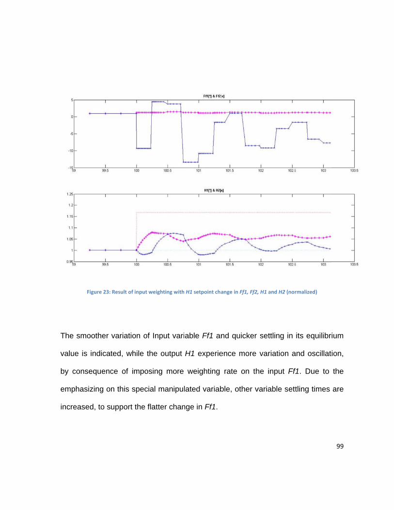
The

valu

by c

emp

incre

Figure 23:

smoother

ue is indica

consequenc

phasizing o

eased, to s

Result of input

variation o

ted, while t

ce of impo

n this spec

upport the

weighting with

f Input vari

the output

osing more

cial manipul

flatter chan

H1 setpoint cha

able Ff1 an

H1 experie

weighting

lated variab

nge in Ff1.

ange in Ff1, Ff2,

nd quicker

ence more

rate on th

ble, other v

, H1 and H2 (no

settling in

variation a

he input Ff

variable set

rmalized)

its equilibr

and oscillat

f1. Due to

tling times

99

ium

ion,

the

are

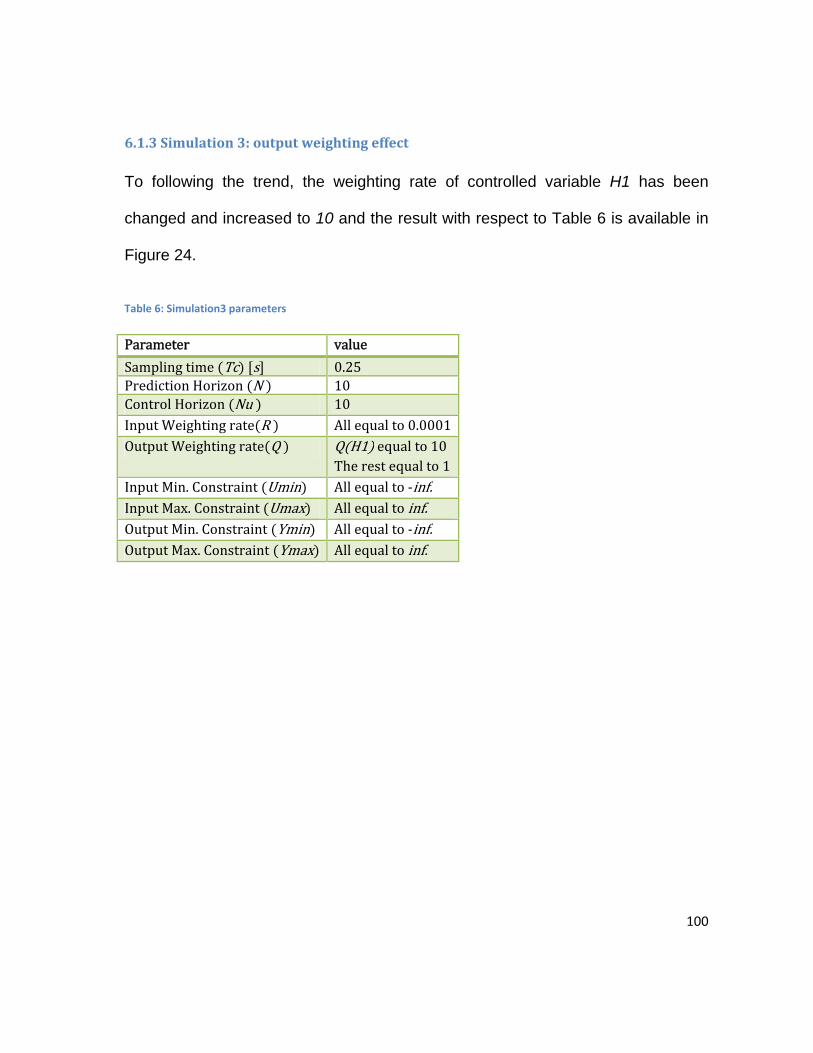
100

6.1.3Simulation3:outputweightingeffect

To following the trend, the weighting rate of controlled variable H1 has been

changed and increased to 10 and the result with respect to Table 6 is available in

Figure 24.


Parameter value

Samplingtime Tc s 0.25PredictionHorizon N 10ControlHorizon Nu 10InputWeightingrate R Allequalto0.0001OutputWeightingrate Q Q H1 equalto10

Therestequalto1InputMin.Constraint Umin Allequalto‐inf.InputMax.Constraint Umax Allequaltoinf.OutputMin.Constraint Ymin Allequalto‐inf.OutputMax.Constraint Ymax Allequaltoinf.

The

quic

integ

Figure 24: R

controlled

ckly, while t

gral action

Result of output

output H1

there is som

in the MPC

t weighting with

1 with highe

me steady s

C controller.

h H1 setpoint ch

er weightin

state error

hange in Ff1, Ff2

g rate, set

which is du

2, H1 and H2 (no

ttled in stea

ue to the u

ormalized)

ady state v

navailability

101

very

y of

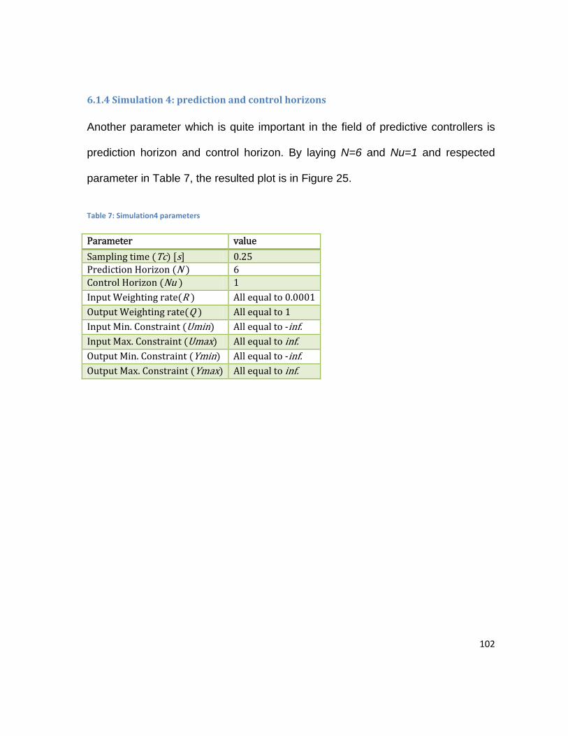
102

6.1.4Simulation4:predictionandcontrolhorizons

Another parameter which is quite important in the field of predictive controllers is

prediction horizon and control horizon. By laying N=6 and Nu=1 and respected

parameter in Table 7, the resulted plot is in Figure 25.


Parameter value

Samplingtime Tc s 0.25PredictionHorizon N 6ControlHorizon Nu 1InputWeightingrate R Allequalto0.0001OutputWeightingrate Q Allequalto1InputMin.Constraint Umin Allequalto‐inf.InputMax.Constraint Umax Allequaltoinf.OutputMin.Constraint Ymin Allequalto‐inf.OutputMax.Constraint Ymax Allequaltoinf.

In th

dram

How

6.1.5

To e

MPC

can

Figure

his case, du

matically an

wever, less

5Simulation

experience

C controller

be presum

25: Result of ho

ue to the s

nd variables

optimizatio

n5:disturba

some distu

r, an initial

med as an

orizons with H1

slighter hori

s experienc

on effort req

anceeffect

urbances a

perturbatio

initial distu

setpoint change

zons of pre

ce more os

quires for co

nd evaluate

on has bee

urbance or

e in Ff1, Ff2, H1

ediction, th

scillation, w

omputation

e the respo

en forced to

r the actua

and H2 (norma

e settling t

which is quit

with reduc

onse of the

o an input v

ator disturba

alized)

ime increas

te predictab

ced horizons

plant with

variable wh

ance. For

103

sed

ble.

s.

the

hich

this

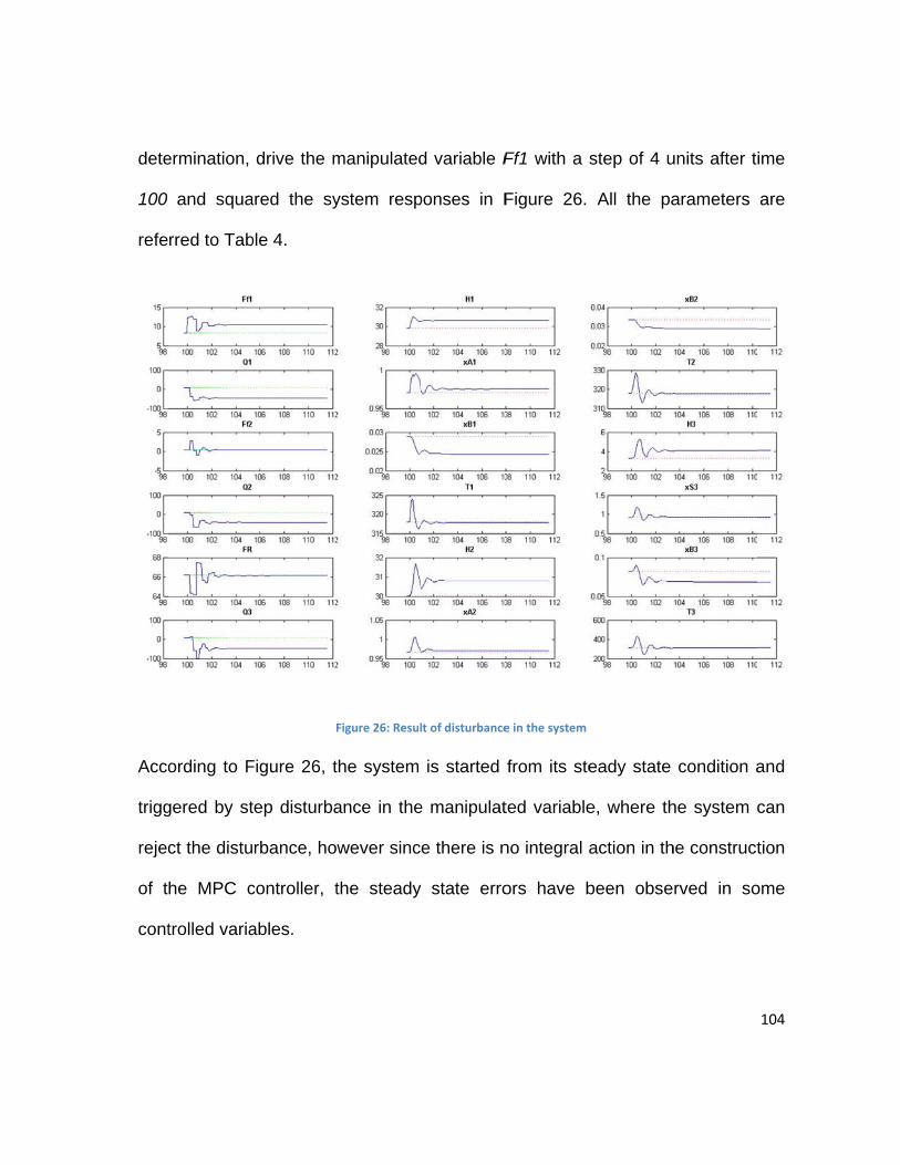
dete

100

refe

Acco

trigg

rejec

of t

cont

ermination,

and squa

rred to Tab

ording to F

gered by st

ct the distu

he MPC c

trolled varia

drive the m

ared the sy

ble 4.

F

Figure 26, t

tep disturba

rbance, ho

controller, t

ables.

manipulated

ystem resp

Figure 26: Resul

the system

ance in the

wever sinc

the steady

d variable F

ponses in F

lt of disturbance

is started

e manipulat

e there is n

y state erro

Ff1 with a s

Figure 26.

e in the system

from its ste

ted variable

no integral a

ors have b

step of 4 u

All the pa

eady state

e, where th

action in th

been obse

units after t

arameters

condition a

he system c

he construct

rved in so

104

ime

are

and

can

tion

ome

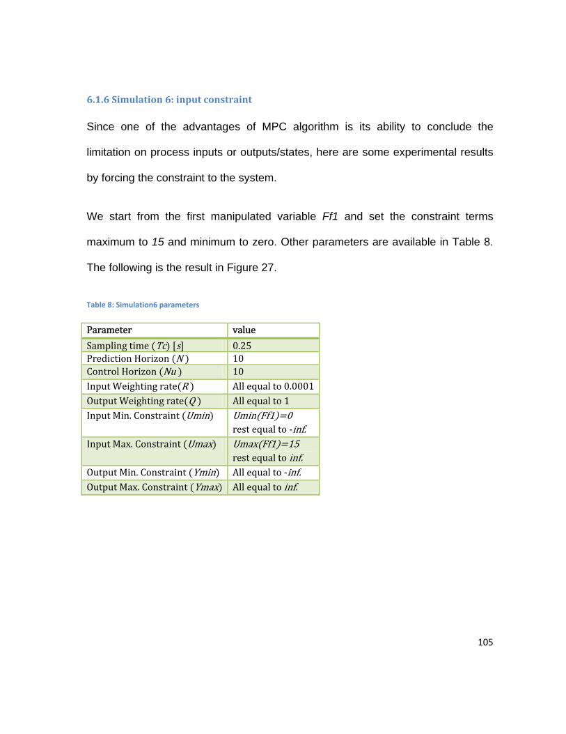
105

6.1.6Simulation6:inputconstraint

Since one of the advantages of MPC algorithm is its ability to conclude the

limitation on process inputs or outputs/states, here are some experimental results

by forcing the constraint to the system.

We start from the first manipulated variable Ff1 and set the constraint terms

maximum to 15 and minimum to zero. Other parameters are available in Table 8.

The following is the result in Figure 27.


Parameter value

Samplingtime Tc s 0.25PredictionHorizon N 10ControlHorizon Nu 10InputWeightingrate R Allequalto0.0001OutputWeightingrate Q Allequalto1InputMin.Constraint Umin Umin Ff1 0

rest equalto‐inf.InputMax.Constraint Umax Umax Ff1 15

rest equaltoinf.OutputMin.Constraint Ymin Allequalto‐inf.OutputMax.Constraint Ymax Allequaltoinf.

So,

varia

6.1.7

Nex

In o

with

com

9.

in compar

able is fluct

7Simulation

xt step is illu

rder to deri

the maxim

mparison to

Figure 27

rison with

tuates in the

n7:outputc

ustrating th

ive the con

mum value

the uncon

7: Result of cons

the uncon

e determine

constraint

e output co

straint, the

set to 325.

strained ca

straint for Ff1 w

nstraint cas

ed range.

onstraint an

temperatu

. The result

ase. Relate

with H1 setpoint

se, as illus

nd its effect

re of first re

t is present

ed paramete

t change

strate in F

t in the sys

eactor (T1)

ted in Figu

ers are refe

igure 27,

stem variab

) is conside

re 28 with

erred to Ta

106

this

les.

ered

the

able

Table

Para

SampPredContInpuOutpInpuInpuOutpOutp

9: Simulation7

ameter

plingtime TdictionHorizotrolHorizonutWeightingputWeightinutMin.ConstrutMax.ConstputMin.ConsputMax.Con

parameters

Tc s on N Nu rate R grate Q raint Umintraint Umaxstraint Yminstraint Yma

Figure 2

value

0.251010AllequaAllequa

Allequax Allequan Allequaax Ymax T

rest equ

8: Result of con

alto0.0001alto1alto‐inf.altoinf.alto‐inf.T1 325ualtoinf.

straint for T1 wwith H1 setpoint change

107

108

6.1.8ConclusiononMPCcontrollerwithoutintegralaction

Within these experiment graphs of the MPC controller without integral action, the

anticipated results have been achieved. The output tuning with new setpoint

worked in the proper way and the controller make the system stable after due

times, however there are some steady state errors according to the non-availability

of the integral action.

Regarding the prediction and control horizons, we can declare that input horizon

can be shorter than prediction (output) horizon, by losing some degree of freedom.

Hence, loss of performance and decreased computational time in the way of

smaller Quadratic Program, are resulted, which is a tradeoff for design the

controller. However in this case, since the constraints are checked up to prediction

horizon, feasibility is maintained.

Input disturbances can be rejected perfectly, within operating region.

Concerning the weight ratio for input and output, it can be concluded that the

larger ratio of output by input weighting, the more aggressive the controller is.

Physical constraints can apply to the controller within MPC method and controller

experience less aggressiveness, when small control deviations have been chosen.

109

6.2ResultsforMPCcontrollerwithintegralaction

Resembling the case of controller without integral action, here we start analysis of

the plant with the constrained MPC algorithm and Integral action. As a general

control tuning analysis method, we apply the step to the setpoint and illustrate the

result in that output trajectory and the influence of this parameter changing, in the

complete system variables, as well.

Noted that MPC controller with the integral action aimed the augmented system in

state space, thus the controller is driven by the state deviation plus output variation

from the setpoint. Consequently, segregation of outputs through states is

conceivable. To employ this benefit, the outputs are defined as [H1, T1, H2, T2,

H3, T3] while the states are remained as [H1, xA1, xB1, T1, H2, xA2, xB2 T2, H3,

xA3, xB3, T3]

6.2.1Simulation8:tuningtheleveloffirstreactor

The leading term in this simulation is the Level of reactor1 (H1), where the step of

5 units in the setpoint makes the following Figures 29, 30, 31. All the significant

parameters are depicted in Table 10.

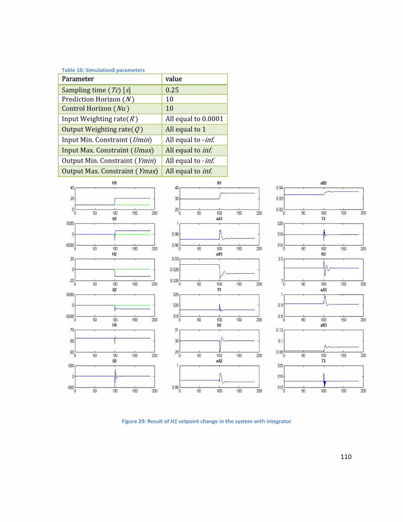
Table

Para


10: Simulation8

ameter


8 parameters


Figure 29: R

value


Allequax Allequan Allequaax Allequa

esult of H1 setp

alto0.0001alto1alto‐inf.altoinf.alto‐inf.altoinf.

point change in tthe system withh integrator

110

Figu

the t

Acco

the

resp

corr

ure 29 illust

time 100, th

F

ording to F

abrupt cha

pect to the

respondingl

trate the tun

he zoomed

Figure 30: Result

igure 30, th

anges in al

weighting

y under the

ning on H1

plot has be

t of H1 setpoint

he change o

l the manip

of that va

e investiga

in the enti

een shown

change in the s

of the setpo

pulated var

riable in th

ation, while

re system.

in Figure 3

system with inte

oint in the le

riables (Ff1

he cost fun

the related

As the ste

30.

egrator‐zoomed

evel of first

1,Q1,Ff2,Q

nction. Outp

d weighting

ep is applied

d

reactor, ma

2,FR,Q3) w

put tracking

g of the out

111

d in

ake

with

g is

tput

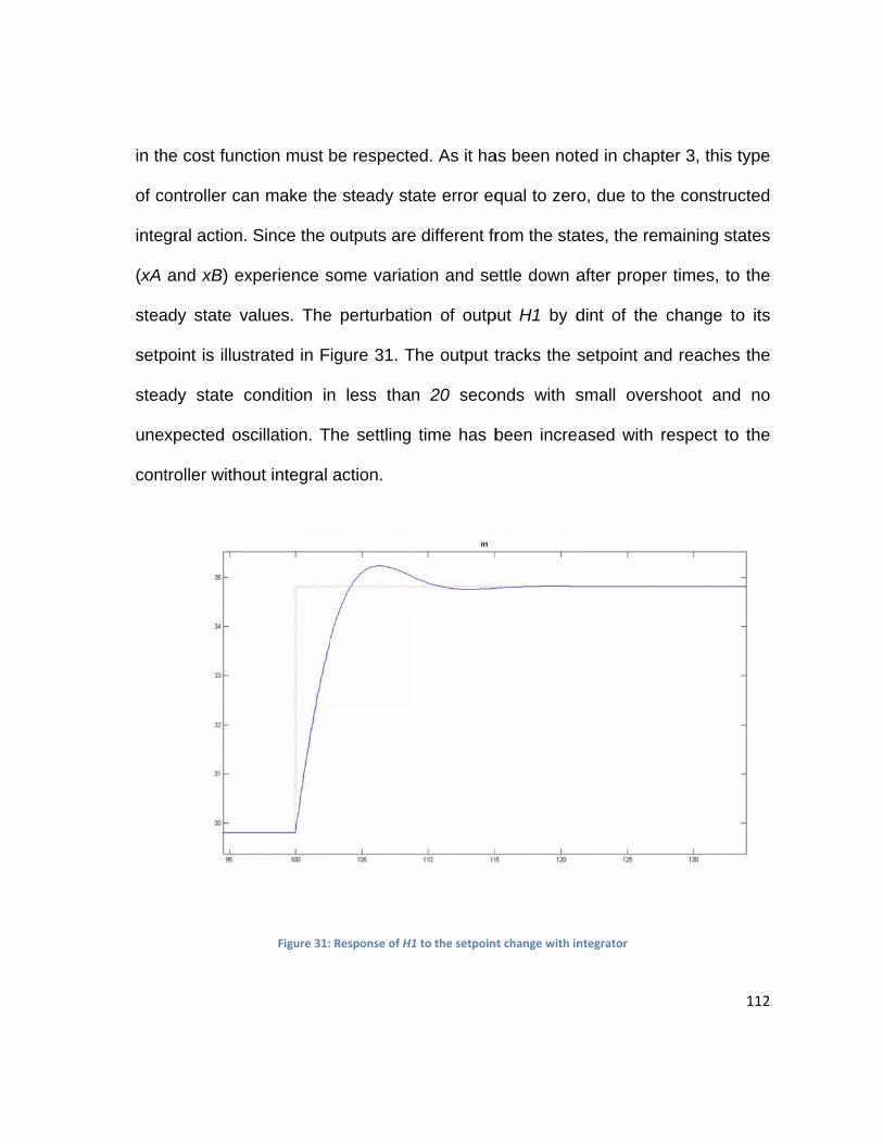
in th

of co

integ

(xA

stea

setp

stea

unex

cont

he cost func

ontroller ca

gral action.

and xB) ex

ady state v

point is illus

ady state c

xpected os

troller witho

ction must b

an make the

Since the o

xperience s

values. The

strated in F

condition in

scillation. T

out integral

Figure 31:

be respecte

e steady st

outputs are

some variat

e perturbati

igure 31. T

n less than

he settling

action.

Response of H1

ed. As it ha

ate error eq

e different fr

tion and se

on of outp

The output t

n 20 seco

time has b

1 to the setpoin

as been not

qual to zero

rom the sta

ettle down a

put H1 by d

tracks the s

onds with s

been increa

nt change with in

ted in chapt

o, due to th

ates, the rem

after prope

dint of the

setpoint an

small overs

ased with

ntegrator

ter 3, this ty

he construc

maining sta

r times, to

change to

nd reaches

shoot and

respect to

112

ype

cted

ates

the

o its

the

no

the

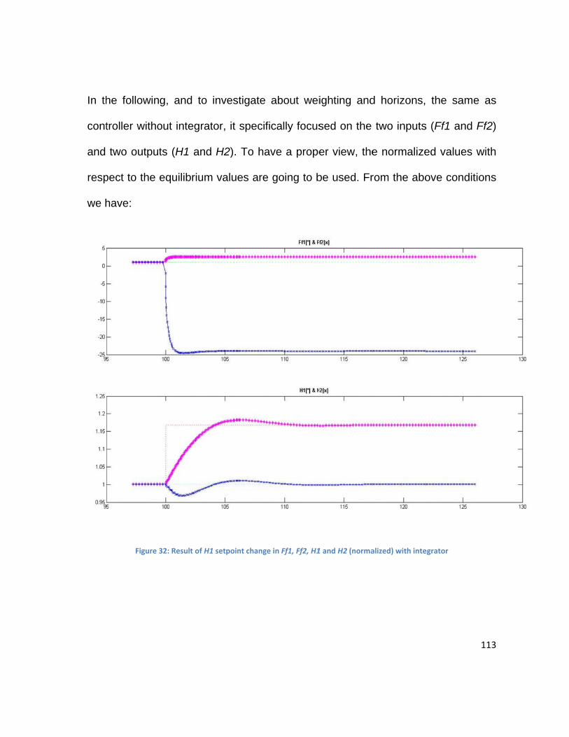
In th

cont

and

resp

we h

he followin

troller witho

two output

pect to the e

have:

Figure 3

g, and to

out integrat

ts (H1 and

equilibrium

32: Result of H1

investigate

tor, it specif

H2). To ha

values are

setpoint chang

about wei

fically focus

ave a prope

e going to b

ge in Ff1, Ff2, H1

ighting and

sed on the

er view, the

be used. Fr

1 and H2 (norma

d horizons,

two inputs

e normalize

rom the abo

alized) with inte

the same

s (Ff1 and F

ed values w

ove conditio

egrator

113

as

Ff2)

with

ons

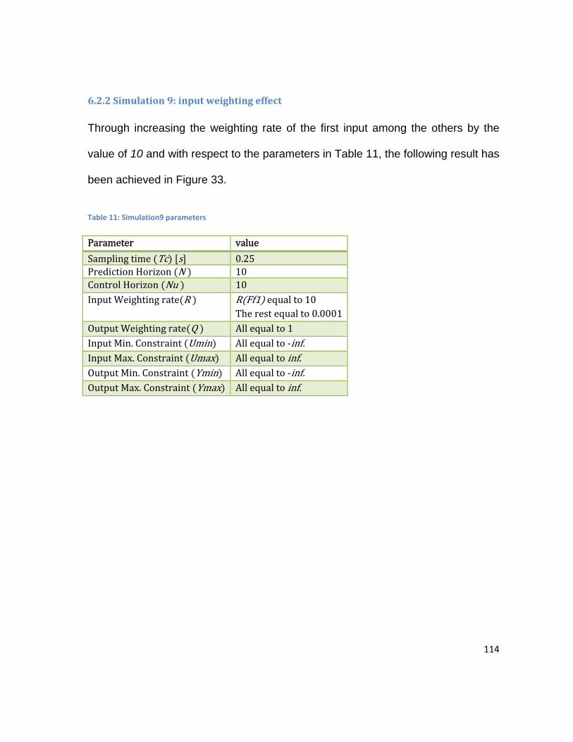
114

6.2.2Simulation9:inputweightingeffect

Through increasing the weighting rate of the first input among the others by the

value of 10 and with respect to the parameters in Table 11, the following result has

been achieved in Figure 33.


Parameter value

Samplingtime Tc s 0.25PredictionHorizon N 10ControlHorizon Nu 10InputWeightingrate R R Ff1 equalto10

Therest equalto0.0001OutputWeightingrate Q Allequalto1InputMin.Constraint Umin Allequalto‐inf.InputMax.Constraint Umax Allequaltoinf.OutputMin.Constraint Ymin Allequalto‐inf.OutputMax.Constraint Ymax Allequaltoinf.

Fig

It in

stea

cons

emp

incre

gure 33: Result o

dicates the

ady state va

sequence

phasizing o

eased, to s

of input weighti

e smoother

alue, while

of imposin

n this spec

upport the

ng with H1 setp

r variation o

the output

ng more w

cial manipul

flatter chan

point change in F

of Input va

t H1 exper

weighting ra

lated variab

nge in Ff1.

Ff1, Ff2, H1 and

ariable Ff1

ience more

ate on the

ble, other v

H2 (normalized

and faster

e time to se

e input Ff1

variable set

d) with integrato

r settling in

ettle down,

1. Due to

tling times

115

or

n its

, by

the

are

116

6.2.3Simulation10:outputweightingeffect

To following the trend, the weighting rate of controlled variable H1 has been

increased and changed to 10 and the result with respect to Table 12 is available is

in Figure 34.


Parameter value

Samplingtime Tc s 0.25PredictionHorizon N 10ControlHorizon Nu 10InputWeightingrate R Allequalto0.0001OutputWeightingrate Q Q H1 equalto10

Therestequalto1InputMin.Constraint Umin Allequalto‐inf.InputMax.Constraint Umax Allequaltoinf.OutputMin.Constraint Ymin Allequalto‐inf.OutputMax.Constraint Ymax Allequaltoinf.

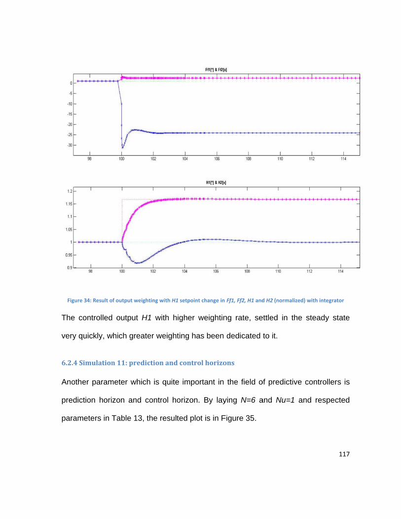
Figu

The

very

6.2.4

Ano

pred

para

ure 34: Result o

controlled

y quickly, w

4Simulation

other param

diction horiz

ameters in T

f output weight

output H1

hich greate

n11:predic

meter which

zon and co

Table 13, th

ting with H1 setp

1 with high

er weighting

ctionandcon

h is quite im

ontrol horiz

he resulted

point change in

er weightin

g has been

ntrolhorizo

mportant in

zon. By lay

plot is in F

Ff1, Ff2, H1 and

ng rate, se

dedicated

ons

the field o

ying N=6 a

Figure 35.

d H2 (normalize

ettled in the

to it.

of predictive

and Nu=1 a

ed) with integrat

e steady st

e controllers

and respec

117

tor

tate

s is

cted

Table

Para


In th

dram

13: Simulation1

ameter


Figure 35: Resu

his case, du

matically an

11 parameters


ult of horizons w

ue to the sl

nd variables

value


Allequax Allequan Allequaax Allequa

with H1 setpoint

lighter horiz

s experienc

alto0.0001alto1alto‐inf.altoinf.alto‐inf.altoinf.

t change in Ff1,

zons for pre

ce more os

Ff2, H1 and H2

ediction, th

scillation, w

(normalized) w

he settling t

which is quit

with integrator

time increas

te predictab

118

sed

ble.

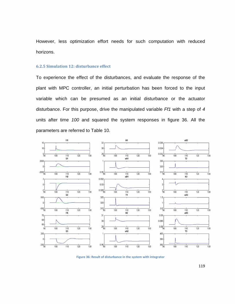
How

horiz

6.2.5

To e

plan

varia

distu

units

para

wever, less

zons.

5Simulation

experience

nt with MP

able which

urbance. Fo

s after tim

ameters are

s optimizat

n12:disturb

the effect

C controlle

h can be

or this purp

e 100 and

e referred to

Figure 3

tion effort

banceeffect

of the dis

er, an initia

presumed

pose, drive

d squared

o Table 10.

6: Result of dist

needs for

t

turbances,

al perturba

as an in

the manip

the system

turbance in the s

r such com

and evalu

ation has b

nitial distu

ulated vari

m respons

system with int

mputation

uate the res

been forced

rbance or

able Ff1 w

es in figur

egrator

with reduc

sponse of

d to the in

the actua

ith a step o

re 36. All

119

ced

the

nput

ator

of 4

the

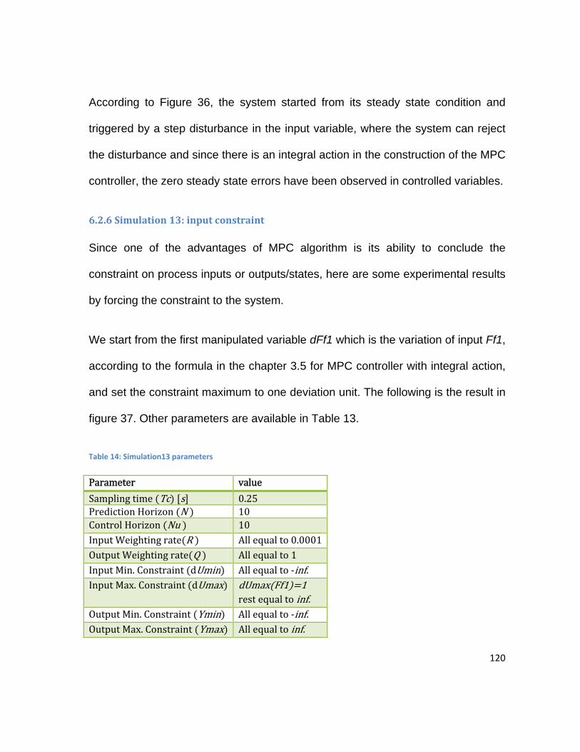
120

According to Figure 36, the system started from its steady state condition and

triggered by a step disturbance in the input variable, where the system can reject

the disturbance and since there is an integral action in the construction of the MPC

controller, the zero steady state errors have been observed in controlled variables.

6.2.6Simulation13:inputconstraint

Since one of the advantages of MPC algorithm is its ability to conclude the

constraint on process inputs or outputs/states, here are some experimental results

by forcing the constraint to the system.

We start from the first manipulated variable dFf1 which is the variation of input Ff1,

according to the formula in the chapter 3.5 for MPC controller with integral action,

and set the constraint maximum to one deviation unit. The following is the result in

figure 37. Other parameters are available in Table 13.


Parameter value

Samplingtime Tc s 0.25PredictionHorizon N 10ControlHorizon Nu 10InputWeightingrate R Allequalto0.0001OutputWeightingrate Q Allequalto1InputMin.Constraint dUmin Allequalto‐inf.InputMax.Constraint dUmax dUmax Ff1 1

rest equaltoinf.OutputMin.Constraint Ymin Allequalto‐inf.OutputMax.Constraint Ymax Allequaltoinf.

whe

has

som

spec

step

6.2.7

Fina

In o

Fi

ere is illustr

been limit

metimes na

cified prope

p.

7Simulation

al step is illu

rder to deri

igure 37: Result

ated that in

ted by its m

amed as “s

erties like a

n14:output

ustrating th

ve the cons

of constraint fo

n the const

maximum d

skew rate”

a pneumatic

tconstraint

he output co

straint, the

or dFf1 with H1 s

trained case

deviation c

”, is mostl

c valve wit

onstraint an

level of sec

setpoint change

e, the varia

constraint. T

ly useful,

h some lim

nd its effect

cond reacto

e with integrato

ation of Ff1

This variati

when the

mits of open

t in the sys

or (H2) is co

or

1 in each st

ion constra

actuator

ning or clos

stem variab

onsidered w

121

tep,

aint,

has

sing

les.

with

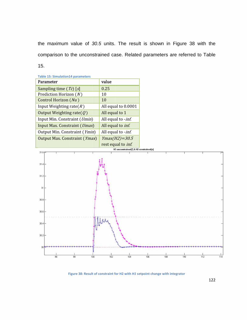
the

com

15.

Table

Para


maximum

mparison to

15: Simulation1

ameter


F

value of 3

the uncon

14 parameters


Figure 38: Result

30.5 units.

strained ca

value


Allequax Allequan Allequaax Ymax H

rest equ

t of constraint fo

The resu

ase. Relate

alto0.0001alto1alto‐inf.altoinf.alto‐inf.H2 30.5ualtoinf.

or H2 with H1 se

lt is shown

ed paramete

etpoint change

n in Figure

ers are refe

with integrator

e 38 with

erred to Ta

r

122

the

able

123

6.2.8ConclusiononMPCcontrollerwithintegralaction

Within these experiment results of the MPC controller with integral action, the

anticipated results have been achieved. The output tuning with new setpoint

worked in the proper way and the controller make the system stable after proper

times which is settled on the setpoint value due to the availability of integral action.

Regarding the prediction and control horizons, we can assert that input horizon

can be shorter than prediction (output) horizon, by losing some degree of freedom.

Hence, loss of performance and decreased computational time with smaller

Quadratic Program, are resulted, which is a tradeoff for design the controller.

However in this case also, since the constrained are checked up to prediction

horizon, feasibility is maintained. Larger control horizon makes the controller to

perform better but increases the complexity. Smaller the prediction horizon derives

the controller to be more aggressive. On the other hand, control variable deviation

constraint can set the controller less aggressive.

Input disturbances can be rejected perfectly, within the operating region.

Concerning the weight ratio for input and output, it can be concluded that the

larger ratio of the output by input weighting (Q/R), make the controller more

aggressive.

124

As the ability to operate a process close to a limiting constraint is an important

objective for advanced process control, for many industrial processes, the

optimum operating condition occurs at a constraint limit. For these situations, the

set point should not be the constraint value because a process disturbance could

force the controlled variable beyond the limit. Thus, the set point should be set

conservatively, based on the ability of the control system to reduce the effects of

disturbances.

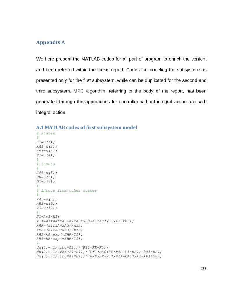
125

AppendixA

We here present the MATLAB codes for all part of program to enrich the content

and been referred within the thesis report. Codes for modeling the subsystems is

presented only for the first subsystem, while can be duplicated for the second and

third subsystem. MPC algorithm, referring to the body of the report, has been

generated through the approaches for controller without integral action and with

integral action.

A.1MATLABcodesoffirstsubsystemmodel% states % H1=u(1); xA1=u(2); xB1=u(3); T1=u(4); % % inputs % Ff1=u(5); FR=u(6); Q1=u(7); % % inputs from other states % xA3=u(8); xB3=u(9); T3=u(10); % F1=kv1*H1; x3s=alfaA*xA3+alfaB*xB3+alfaC*(1-xA3-xB3); xAR=(alfaA*xA3)/x3s; xBR=(alfaB*xB3)/x3s; kA1=kA*exp(-EAR/T1); kB1=kB*exp(-EBR/T1); % dx(1)=(1/(rho*A1))*(Ff1+FR-F1); dx(2)=(1/(rho*A1*H1))*(Ff1*xA0+FR*xAR-F1*xA1)-kA1*xA1; dx(3)=(1/(rho*A1*H1))*(FR*xBR-F1*xB1)+kA1*xA1-kB1*xB1;

126

dx(4)=(1/(rho*A1*H1))*(Ff1*T0+FR*TR-F1*T1)-(1/Cp)*(kA1*xA1*DHA+kB1*xB1*DHB)+Q1/(rho*A1*Cp*H1); dx(5)=F1;

A.2MATLABcodes forpreparationofMPCparameterswithout integralactionTc=.25; [A,B]=c2d(AA,BB,Tc); C=CC; [n,m]=size(B); [p,n]=size(C); M=zeros(n,1); d=1; % R=diag([1.10 0.000010 0.000010 0.000010 0.000010 0.000010]); QY=diag([10 1 1 1 1 1 1 1 1 1 1 1]); Q=C'*QY*C; [K,P,E] = DLQR(A,B,Q,R); S=P; SY=eye(p); % umin=[-1000000 ; -1000000; -1000000 ; -1000000 ; -1000000 ; -1000000]; umax=[1000000 ; 1000000 ; 1000000 ; 1000000 ; 1000000 ; 1000000]; % ymin=[-1000000 ; -1000000 ; -1000000 ;-1000000; -1000000 ; -1000000; -1000000; -1000000; -1000000; -1000000; -1000000; -1000000]; ymax=[1000000 ; 1000000; 1000000; 1000000; 1000000 ; 1000000; 1000000; 1000000; 1000000; 1000000; 1000000; 1000000 ]; % Np=10; Nu=10; % % construction of matrices for quadprog of output % H=2*(CBT'*QTY*CBT+RT); D=zeros(Np*d,1);

A.3MATLABcodesforconstructionofmatrixeswithoutintegralaction% construct the matrices for predictive control of linear systems % A,B : matrix of the system (possibly extended first with integrators) % Q, S, QY, SY, R : weight matrices of state, final state, output, final output, control % Np, Nu : horizons of prediction and control % umin,umax, dumin,dumax : limits on the values ??of control and variation % of control [n,n]=size(A);

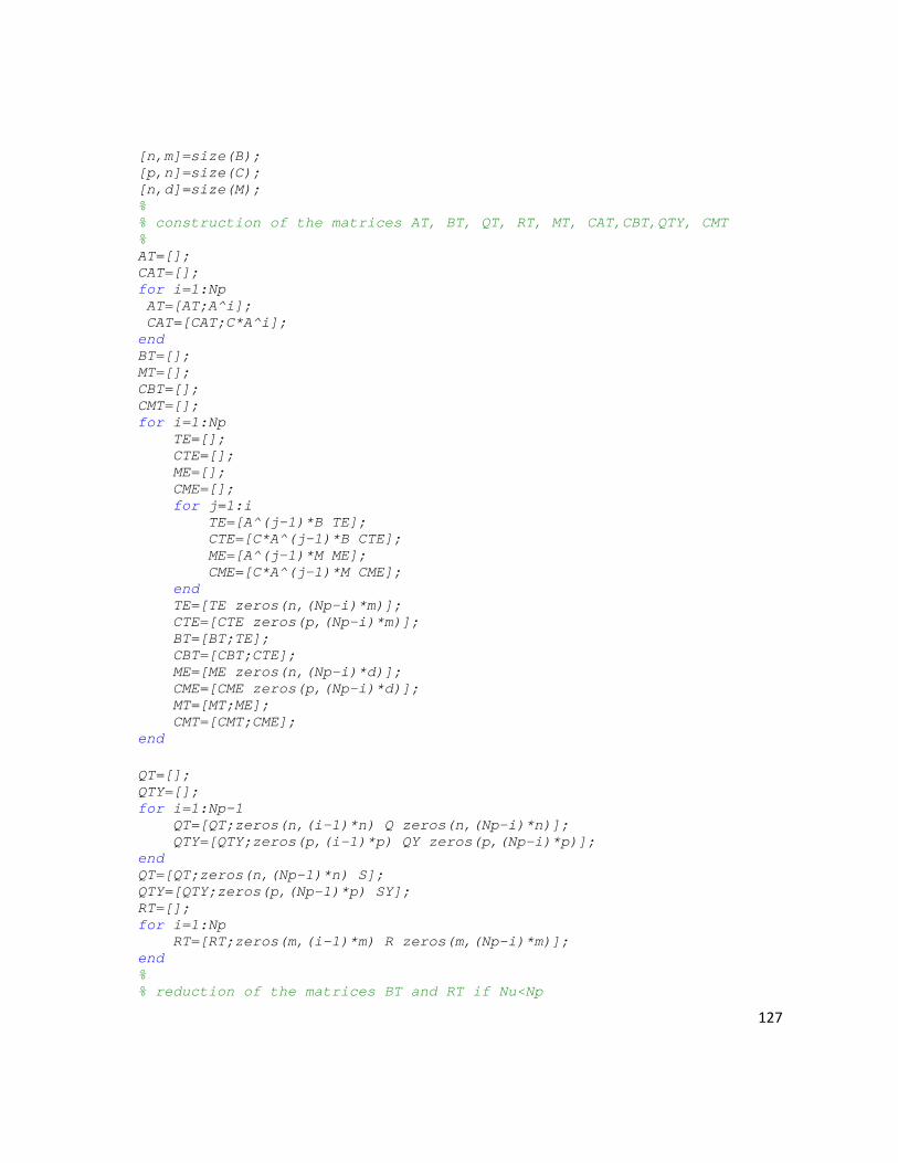
127

[n,m]=size(B); [p,n]=size(C); [n,d]=size(M); % % construction of the matrices AT, BT, QT, RT, MT, CAT,CBT,QTY, CMT % AT=[]; CAT=[]; for i=1:Np AT=[AT;A^i]; CAT=[CAT;C*A^i]; end BT=[]; MT=[]; CBT=[]; CMT=[]; for i=1:Np TE=[]; CTE=[]; ME=[]; CME=[]; for j=1:i TE=[A^(j-1)*B TE]; CTE=[C*A^(j-1)*B CTE]; ME=[A^(j-1)*M ME]; CME=[C*A^(j-1)*M CME]; end TE=[TE zeros(n,(Np-i)*m)]; CTE=[CTE zeros(p,(Np-i)*m)]; BT=[BT;TE]; CBT=[CBT;CTE]; ME=[ME zeros(n,(Np-i)*d)]; CME=[CME zeros(p,(Np-i)*d)]; MT=[MT;ME]; CMT=[CMT;CME]; end QT=[]; QTY=[]; for i=1:Np-1 QT=[QT;zeros(n,(i-1)*n) Q zeros(n,(Np-i)*n)]; QTY=[QTY;zeros(p,(i-1)*p) QY zeros(p,(Np-i)*p)]; end QT=[QT;zeros(n,(Np-1)*n) S]; QTY=[QTY;zeros(p,(Np-1)*p) SY]; RT=[]; for i=1:Np RT=[RT;zeros(m,(i-1)*m) R zeros(m,(Np-i)*m)]; end % % reduction of the matrices BT and RT if Nu<Np

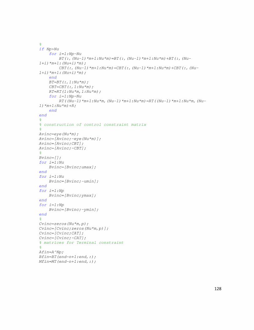
128

% if Np>Nu for i=1:Np-Nu BT(:,(Nu-1)*m+1:Nu*m)=BT(:,(Nu-1)*m+1:Nu*m)+BT(:,(Nu-1+i)*m+1:(Nu+i)*m); CBT(:,(Nu-1)*m+1:Nu*m)=CBT(:,(Nu-1)*m+1:Nu*m)+CBT(:,(Nu-1+i)*m+1:(Nu+i)*m); end BT=BT(:,1:Nu*m); CBT=CBT(:,1:Nu*m); RT=RT(1:Nu*m,1:Nu*m); for i=1:Np-Nu RT((Nu-1)*m+1:Nu*m,(Nu-1)*m+1:Nu*m)=RT((Nu-1)*m+1:Nu*m,(Nu-1)*m+1:Nu*m)+R; end end % % construction of control constraint matrix % Avinc=eye(Nu*m); Avinc=[Avinc;-eye(Nu*m)]; Avinc=[Avinc;CBT]; Avinc=[Avinc;-CBT]; % Bvinc=[]; for i=1:Nu Bvinc=[Bvinc;umax]; end for i=1:Nu Bvinc=[Bvinc;-umin]; end for i=1:Np Bvinc=[Bvinc;ymax]; end for i=1:Np Bvinc=[Bvinc;-ymin]; end % Cvinc=zeros(Nu*m,p); Cvinc=[Cvinc;zeros(Nu*m,p)]; Cvinc=[Cvinc;CAT]; Cvinc=[Cvinc;-CAT]; % matrices for Terminal constraint % Afin=A^Np; Bfin=BT(end-n+1:end,:); Mfin=MT(end-n+1:end,:);

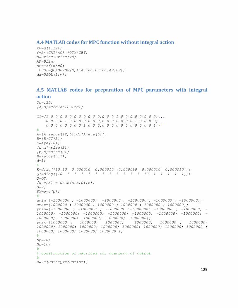
129

A.4MATLABcodesforMPCfunctionwithoutintegralactionx0=u(1:12); f=2*(CAT*x0)'*QTY*CBT; b=Bvinc+Cvinc*x0; AF=Bfin; BF=-Afin*x0; USOL=QUADPROG(H,f,Avinc,Bvinc,AF,BF); dx=USOL(1:m);

A.5 MATLAB codes for preparation of MPC parameters with integralactionTc=.25; [A,B]=c2d(AA,BB,Tc); CI=[1 0 0 0 0 0 0 0 0 0 0 0;0 0 0 1 0 0 0 0 0 0 0 0;... 0 0 0 0 1 0 0 0 0 0 0 0;0 0 0 0 0 0 0 1 0 0 0 0;... 0 0 0 0 0 0 0 0 1 0 0 0;0 0 0 0 0 0 0 0 0 0 0 1]; % A=[A zeros(12,6);CI*A eye(6)]; B=[B;CI*B]; C=eye(18); [n,m]=size(B); [p,n]=size(C); M=zeros(n,1); d=1; % R=diag([10.10 0.000010 0.000010 0.000010 0.000010 0.000010]); QY=diag([10 1 1 1 1 1 1 1 1 1 1 1 10 1 1 1 1 1]); Q=QY; [K,P,E] = DLQR(A,B,QY,R); S=P; SY=eye(p); % umin=[-1000000 ; -1000000; -1000000 ; -1000000 ; -1000000 ; -1000000]; umax=[1000000 ; 1000000 ; 1000000 ; 1000000 ; 1000000 ; 1000000]; ymin=[-1000000 ; -1000000 ; -1000000 ;-1000000; -1000000 ; -1000000; -1000000; -1000000; -1000000; -1000000; -1000000; -1000000; -1000000; -1000000; -1000000; -1000000; -1000000; -1000000]; ymax=[1000000 ; 1000000; 1000000; 1000000; 1000000 ; 1000000; 1000000; 1000000; 1000000; 1000000; 1000000; 1000000; 1000000; 1000000 ; 1000000; 1000000; 1000000; 1000000 ]; % Np=10; Nu=10; % % construction of matrices for quadprog of output % H=2*(CBT'*QTY*CBT+RT);

130

D=zeros(Np*d,1);

A.6MATLABcodesforconstructionofmatrixeswithintegralaction % construct the matrices for predictive control of linear systems % A,B : matrix of the system (possibly extended first with integrators) % Q, S, QY, SY, R : weight matrices of state, final state, output, final output, control % Np, Nu : horizons of prediction and control % umin,umax, dumin,dumax : limits on the values ??of control and variation % of control [n,n]=size(A); [n,m]=size(B); [p,n]=size(C); [n,d]=size(M); % % construction of the matrices AT, BT, QT, RT, MT, CAT,CBT,QTY, CMT % AT=[]; CAT=[]; for i=1:Np AT=[AT;A^i]; CAT=[CAT;C*A^i]; end BT=[]; MT=[]; CBT=[]; CMT=[]; for i=1:Np TE=[]; CTE=[]; ME=[]; CME=[]; for j=1:i TE=[A^(j-1)*B TE]; CTE=[C*A^(j-1)*B CTE]; ME=[A^(j-1)*M ME]; CME=[C*A^(j-1)*M CME]; end TE=[TE zeros(n,(Np-i)*m)]; CTE=[CTE zeros(p,(Np-i)*m)]; BT=[BT;TE]; CBT=[CBT;CTE]; ME=[ME zeros(n,(Np-i)*d)]; CME=[CME zeros(p,(Np-i)*d)]; MT=[MT;ME]; CMT=[CMT;CME];

131

end QT=[]; QTY=[]; for i=1:Np-1 QT=[QT;zeros(n,(i-1)*n) Q zeros(n,(Np-i)*n)]; QTY=[QTY;zeros(p,(i-1)*p) QY zeros(p,(Np-i)*p)]; end QT=[QT;zeros(n,(Np-1)*n) S]; QTY=[QTY;zeros(p,(Np-1)*p) SY]; RT=[]; for i=1:Np RT=[RT;zeros(m,(i-1)*m) R zeros(m,(Np-i)*m)]; end % % reduction of the matrices BT and RT if Nu<Np % if Np>Nu for i=1:Np-Nu BT(:,(Nu-1)*m+1:Nu*m)=BT(:,(Nu-1)*m+1:Nu*m)+BT(:,(Nu-1+i)*m+1:(Nu+i)*m); CBT(:,(Nu-1)*m+1:Nu*m)=CBT(:,(Nu-1)*m+1:Nu*m)+CBT(:,(Nu-1+i)*m+1:(Nu+i)*m); end BT=BT(:,1:Nu*m); CBT=CBT(:,1:Nu*m); RT=RT(1:Nu*m,1:Nu*m); for i=1:Np-Nu RT((Nu-1)*m+1:Nu*m,(Nu-1)*m+1:Nu*m)=RT((Nu-1)*m+1:Nu*m,(Nu-1)*m+1:Nu*m)+R; end end % % construction of control constraint matrix % Avinc=eye(Nu*m); Avinc=[Avinc;-eye(Nu*m)]; Avinc=[Avinc;CBT]; Avinc=[Avinc;-CBT]; % Bvinc=[]; for i=1:Nu Bvinc=[Bvinc;umax]; end for i=1:Nu Bvinc=[Bvinc;-umin]; end for i=1:Np Bvinc=[Bvinc;ymax]; end for i=1:Np

132

Bvinc=[Bvinc;-ymin]; end % Cvinc=zeros(Nu*m,p); Cvinc=[Cvinc;zeros(Nu*m,p)]; Cvinc=[Cvinc;-CAT]; Cvinc=[Cvinc;CAT]; % matrices for Terminal constraint % Afin=A^Np; Bfin=BT(end-n+1:end,:); Mfin=MT(end-n+1:end,:);

A.7MATLABcodesforMPCfunctionwithintegralactionx0=u(1:18); f=2*(CAT*x0)'*QTY*CBT; b=Bvinc+Cvinc*x0; AF=Bfin; BF=-Afin*x0; USOL=QUADPROG(H,f,Avinc,b,AF,BF); dx=USOL(1:m);

133

Bibliography

[1] J. M. Maciejowski: “Predictive Control with Constraints”, Prentice Hall, 2001.

[2] R. Scattolini, “Lecture Notes for SIDRA Summer School 2011 on Model Predictive Control”, ftp://ftp.elet.polimi.it/outgoing/Riccardo.Scattolini /Bertinoro2011_controllo_predittivo/

[3] C.E. Garcia, D.M. Prett, M. Morari: “Model predictive control: theory and practice – a survey”, Automatica, Vol. 25, n. 3, pp. 335-348, 1989.

[4] D.Q. Mayne, J.B. Rawlings, C.V. Rao, P.O. Scokaert: “Constrained model predictive control: stability and optimality”, Automatica, Vol. 36, pp. 789-814, 2000.

[5] B.T. Stewart, A.N. Venkat, J. B. Rawlings, S. J. Wright, G. Pannocchia: “Cooperative distributed model predictive control “, Systems & Control Letters 59 (2010) 460_469.

[6] D.E. Seborg, T.F. Edgar, D.A. Mellichamp: “Process dynamics and control”, John Wiley & Sons, 2004.

[7] M.J. Willis: “Continuous stirred tank reactor models”, Dept. of Chemical and Process Eng., Uni. of Newcastle, 2000.

[8] S.J. Qin, T.A. Badgwell: “A survey of industrial model predictive control technology”, Control Engineering Practice, Vol. 11, n. 7, pp. 733-764.

[9] M. Bauer, I.K. Craig: “Economic assessment of advanced process control – A survey and framework”, Journal of Process Control, Vol. 18, n. 1, pp. 2-18, 2008.

[10] M. Kano, M. Ogawa: “The state of the art in chemical process control in Japan: Good practice and questionnaire survey”, Journal of Process Control 20 (2010) 969–982.

[11] J.A. Rossiter: “Model based predictive control: a practical approach”, CRC Press, 2003.

134

[12] M. Morari, J. H. Lee: “Model predictive control: past, present and future”, Computers and Chemical Engineering, Vol. 23, n. 4-5, pp. 667-682, 1999.

[13] J.A. Richalet, A. Rault, J.D. Testud, J. Papon: “Model predictive heuristic control: applications to industrial processes”, Automatica, Vol. 14, pp. 413-428, 1978.

[14] M.L. Luyben, W.L. Luybed: “Design and Control of a Complex Process Involving Two Reaction Steps, Three Distillation Columns, and Two Recycle Streams” , Ind. Eng. Chem. Res. 1996,34, 3885-3898.

[15] B. Wayne: “Nonlinear Control of Chemical Processes: A Review”, Ind. Eng. Chem. Res. 1991, 30, 1391-1413.

[16] P.B. Sistu, B. Wayne: “Nonlinear Predictive Control of Uncertain Processes: Application to a CSTR”, AIChE Journal, 1991, Vol. 37, No. 11.

NICO DI MILAN ANO · I would also like to take this opportunity to thank Prof. Sergio Bittanti and...

Documents

Transcript of NICO DI MILAN ANO · I would also like to take this opportunity to thank Prof. Sergio Bittanti and...