NGN Cost Modelling - report by csmg

CSMG Confidential and Proprietary.

© 2012 CSMG. No part of this publication may be reproduced, stored in a retrieval system, or transmitted in any form or means (electronic, mechanical, photocopy, recording or otherwise) without the permission of CSMG.

Fixed Narrowband Market Review: NGN Cost Modelling

Model Documentation

v1.0

Prepared for:

Prepared by:

CSMG Descartes House 8 Gate Street London WC2A 3HP United Kingdom www.csmg-global.com

27 September 2012

2 V1.0

Table of Contents

1. Introduction ......................................................................................................................... 3

2. Scope ................................................................................................................................... 4

Technology .................................................................................................................................... 4

Geography ..................................................................................................................................... 4

Services.......................................................................................................................................... 4

Timeframe ..................................................................................................................................... 4

Existing Assets ............................................................................................................................... 5

3. Network Architecture ........................................................................................................... 6

Overview ....................................................................................................................................... 6

Access Node Categorisation .......................................................................................................... 7

Basic Access Node ......................................................................................................................... 7

Remote Access Node ..................................................................................................................... 8

Super Access Node ........................................................................................................................ 9

Aggregation Node ....................................................................................................................... 10

Interconnect Node ...................................................................................................................... 11

Service Node ............................................................................................................................... 12

Core Node ................................................................................................................................... 13

Example of Co-location ............................................................................................................... 14

Call Pathways for Modelled Services .......................................................................................... 14

4. Model Implementation and Assumptions ............................................................................ 16

Overview of Network and Cost Modules .................................................................................... 16

Network Module ......................................................................................................................... 16

Cost Module ................................................................................................................................ 20

5. Glossary ............................................................................................................................. 24

6. Appendix A: Core Node Architecture ................................................................................... 25

3 V1.0

1. INTRODUCTION

1.1 In June 2012, Ofcom commissioned CSMG to develop a network cost model in support of Ofcom’s Fixed Narrowband Market Review. The purpose of the model is to assist Ofcom in estimating the efficient costs of providing wholesale narrowband services.

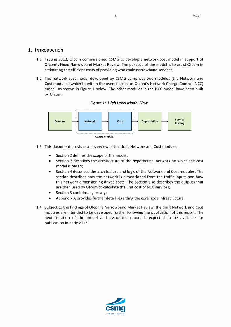
1.2 The network cost model developed by CSMG comprises two modules (the Network and Cost modules) which fit within the overall scope of Ofcom’s Network Charge Control (NCC) model, as shown in Figure 1 below. The other modules in the NCC model have been built by Ofcom.

Figure 1: High Level Model Flow

1.3 This document provides an overview of the draft Network and Cost modules:

Section 2 defines the scope of the model;

Section 3 describes the architecture of the hypothetical network on which the cost model is based;

Section 4 describes the architecture and logic of the Network and Cost modules. The section describes how the network is dimensioned from the traffic inputs and how this network dimensioning drives costs. The section also describes the outputs that are then used by Ofcom to calculate the unit cost of NCC services;

Section 5 contains a glossary;

Appendix A provides further detail regarding the core node infrastructure.

1.4 Subject to the findings of Ofcom’s Narrowband Market Review, the draft Network and Cost modules are intended to be developed further following the publication of this report. The next iteration of the model and associated report is expected to be available for publication in early 2013.

4 V1.0

2. SCOPE

Technology

2.1 The cost model represents a hypothetical Next-Generation Network (NGN) in which multiple services are transported over a shared Internet Protocol (IP) network.

2.2 The access network is not modelled. Access lines are assumed to be copper-based.

Geography

2.3 The geographical scope of the model is based on the coverage area of BT’s current exchange footprint in the United Kingdom. This includes locations in England, Wales, Scotland and Northern Ireland, with the exception of Hull.

Services

2.4 The modelled NGN supports voice and data services. The network is dimensioned on a bottom-up basis from demand forecasts for voice and broadband access.

2.5 Voice services on the network emulate the Public Switched Telephony Network (PSTN) with both analogue and Integrated Services Digital Network (ISDN) access. Interconnection for voice services with other Communication Providers (CPs) includes both Time Division Multiplexing (TDM) and IP based interconnects.

2.6 The model considers voice calls in which both the originating and terminating lines are on the NGN (“on net”), and calls in which one end of the call is on another CP’s network (“off net”).

2.7 We consider both retail and wholesale voice services in the model. Retail voice services are provided by the modelled CP directly to its end customers. Wholesale voice services comprise wholesale access and wholesale calls. Wholesale voice access enables a CP to interconnect with the modelled network and use the access segment of the network to reach their own customers. In wholesale calls, the modelled network is also used for call conveyance. Broadband access also encompasses retail and wholesale services. Wholesale broadband access enables a CP to interconnect with the modelled network and use the access segment of the network to reach their own customers.

2.8 Capacity requirements for Leased Lines are modelled using a top-down approach.

Timeframe

2.9 Time periods in the model are financial years (April to March). The model considers a 40 year period from 2005/06 to 2045/46.

2.10 We assume network build to start in 2005/06. During the network build phase a number of exchanges are added to the NGN each year until all exchanges have been covered. This build process is assumed to take 10 years, up until the end of 2014/15.

5 V1.0

Existing Assets

2.11 The network module employs a scorched node approach. The location and serving area of BT’s exchanges is preserved, however the function of and network elements in each exchange are driven only by the model and not actual, existing network deployment.

2.12 All nodes are assumed to require each of the following:

DC power, battery back-up and generator

AC power and Uninterrupted Power System (UPS)

Air Conditioning

Security

Environmental Alarms

Fire suppressant

Cable management

Management network

2.13 These “property” costs are not modelled individually on a bottom-up basis. Instead, an average capital cost per rack is estimated and applied proportionally to the network equipment based on rack space occupancy. We calculate the ongoing costs as a percentage of the upfront capital cost and apply them proportionally in the same manner.

2.14 Costs for duct and fibre are included in the cost module, however these costs do not form part of the bottom-up analysis. They are applied later as a mark-up in Ofcom’s service costing module.

6 V1.0

3. NETWORK ARCHITECTURE

Overview

3.1 The modelled NGN comprises of a series of interconnected logical nodes. Each of these node types performs specific functions which are described in the remainder of this section.

3.2 Figure 2 provides an overview of the network architecture showing the relationship between the logical nodes.

Figure 2: NGN Network Logical Architecture1

3.3 The modelled network supports multiple services on a common infrastructure. Voice and data services are supported for both residential and business customers.

3.4 The network is designed for high-availability, consistent with the expectations for PSTN voice services (typically 99.999% availability). General principles of the network architecture are that:

Nodes are dual-parented, providing redundant network pathways to protect against the failure of a node.

Multiple connections are used between nodes with diverse paths to protect against cable breaks. In the majority of cases ring topologies are used to redundantly connect multiple nodes. Two diversely routed point-to-point connections are used for small, remote access nodes where a ring would be cost-prohibitive.

Network electronics are dimensioned to allow for traffic to be rerouted in failure conditions. This includes duplication of components within network elements (e.g. control units, switch fabrics and high-bandwidth interfaces) and in some cases duplication of the network element itself.

3.5 In line with industry norms, the modelled NGN is based on IP technology. For cost efficiency, the underlying transmission network is Ethernet based. Between sites, Dense

1 See Appendix A for discussion on the connectivity between core nodes

7 V1.0

Wavelength Division Multiplexing (DWDM) over fibre has been selected for high-capacity and future scalability. The DWDM connections are implemented using Optical Transport Network (OTN) equipment. We have used OTN as the basis of our cost modelling as the data is available to us for this equipment.

3.6 Multi-Protocol Label Switching (MPLS) is used in the core network. MPLS enables connection-oriented paths to be established across a connectionless (e.g. IP) network which facilitates Quality of Service (QoS) management and capacity planning.

Access Node Categorisation

3.7 Access nodes are the locations which aggregate physical access connections from end-users. There are approximately 5,600 access nodes, which correspond to MDF sites (Main Distribution Frame sites, also known as local exchanges) on BT’s network.

3.8 Access nodes are segmented into 10 categories. The categories are based on the characteristics of each exchange in relation to the split of residential/business premises and the total number of residential premises served.

3.9 There is a degree of co-location between logical nodes in the network. Given the hierarchy of Basic Access Node > Super Access Node > Aggregation Node > Core Node, the co-location rule is such that every parent node will be co-located with a ‘child’ node. For example, every Core Node is co-located with an Aggregation Node.

3.10 Physical sites in the network have the combined functionality of all the logical nodes located at that site.

Basic Access Node

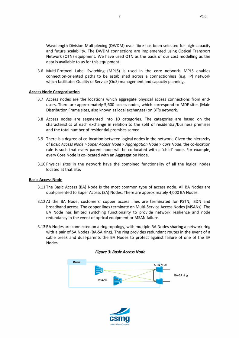
3.11 The Basic Access (BA) Node is the most common type of access node. All BA Nodes are dual-parented to Super Access (SA) Nodes. There are approximately 4,000 BA Nodes.

3.12 At the BA Node, customers’ copper access lines are terminated for PSTN, ISDN and broadband access. The copper lines terminate on Multi-Service Access Nodes (MSANs). The BA Node has limited switching functionality to provide network resilience and node redundancy in the event of optical equipment or MSAN failure.

3.13 BA Nodes are connected on a ring topology, with multiple BA Nodes sharing a network ring with a pair of SA Nodes (BA-SA ring). The ring provides redundant routes in the event of a cable break and dual-parents the BA Nodes to protect against failure of one of the SA Nodes.

Figure 3: Basic Access Node

8 V1.0

Key Elements

3.14 Multi-Service Access Node (MSAN): The MSAN terminates copper lines for PSTN, ISDN and broadband services. It acts as a gateway, adapting the data and signalling for these services into IP packets for the NGN (and vice versa). The MSAN has a Gigabit Ethernet interface for IP traffic. Voice and data traffic is kept logically separate on this interface using Virtual Local Area Network (VLAN) tags.

3.15 VLAN tagging allows for differential QoS treatment of different traffic types (e.g. voice, data) by the separation of one physical network into multiple independent logical networks. This allows for PSTN-quality management of voice services over the shared physical network.

3.16 Optical Transport Network (OTN) Multiplexer: The OTN Multiplexer enables multiple point-to-point connections to be set up over a fibre ring. The OTN provides Gigabit Ethernet ports for connection to the MSANs and 10Gbps Ethernet ports for aggregating the traffic on the ring.

Remote Access Node

3.17 The Remote Access (RA) Node is a special type of access node that serves small and/or remote communities. The RA Node serves the same function as the BA Node, but due its geographic location it is not connected to the Super Access Node on a ring topology. Instead, two diversely routed point-to-point connections are used. Based on the distribution of BT exchange sites, the model assumes there are 1,600 RA Nodes.

3.18 500 of the RA Nodes are assumed to be located in areas (e.g. highlands and islands) with a higher risk of prolonged network failure. In these cases, the RA Nodes incorporate a small Softswitch to maintain local voice services in the event that the node becomes isolated from the rest of the network. This is consistent with the design of BT’s 21CN voice network which sought to emulate the function currently provided by UXD5 switches at these locations in BT’s TDM network.

Figure 4: Remote Access Node and Corresponding Super Access Node

9 V1.0

Key Elements

3.19 Softswitch: A Voice over IP (VoIP) switch that is able to route voice calls and thus support local voice services in the event that the RA Node becomes isolated. The soft switch interoperates with the call servers in the core network under normal operation. This softswitch is only present in 500 of the 1,600 RA Nodes in the network.

3.20 Ethernet Switch: There is a redundant pair of Ethernet switches in the RA Node. The Ethernet switches provide connectivity within the RA Node between the MSAN, soft switch and optical line system.

3.21 Optical Line System: The optical line system provides point-to-point Ethernet connectivity between the RA Node and the SA Node. The optical line system takes the place of the ring-based DWDM equipment used in the BA Node as a ring-based topology is unlikely to be cost-effective for remote locations.

3.22 Multi-Service Access Node (MSAN): (as above).

Super Access Node

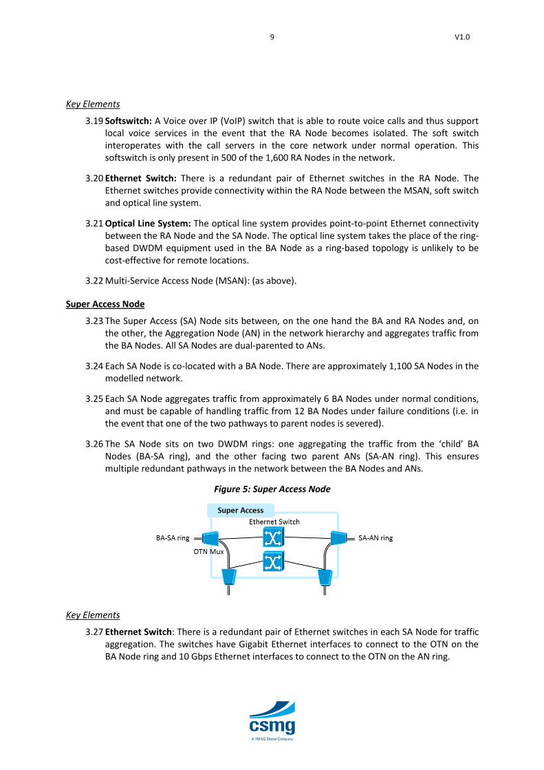
3.23 The Super Access (SA) Node sits between, on the one hand the BA and RA Nodes and, on the other, the Aggregation Node (AN) in the network hierarchy and aggregates traffic from the BA Nodes. All SA Nodes are dual-parented to ANs.

3.24 Each SA Node is co-located with a BA Node. There are approximately 1,100 SA Nodes in the modelled network.

3.25 Each SA Node aggregates traffic from approximately 6 BA Nodes under normal conditions, and must be capable of handling traffic from 12 BA Nodes under failure conditions (i.e. in the event that one of the two pathways to parent nodes is severed).

3.26 The SA Node sits on two DWDM rings: one aggregating the traffic from the ‘child’ BA Nodes (BA-SA ring), and the other facing two parent ANs (SA-AN ring). This ensures multiple redundant pathways in the network between the BA Nodes and ANs.

Figure 5: Super Access Node

Key Elements

3.27 Ethernet Switch: There is a redundant pair of Ethernet switches in each SA Node for traffic aggregation. The switches have Gigabit Ethernet interfaces to connect to the OTN on the BA Node ring and 10 Gbps Ethernet interfaces to connect to the OTN on the AN ring.

10 V1.0

3.28 Synchronisation (Sync) Source: Each SA Node has a local sync source to distribute a network clock signal to the MSANs in the child BA Nodes. The MSANs require accurate timing for fax and modem support. The sync sources in the SA Nodes are fed by three master sync sources in the core of the network.

3.29 OTN Multiplexer (as above).

Aggregation Node

3.30 The Aggregation Node (AN) sits between the SA Nodes and Core Nodes. Each AN is co-located with a SA Node. All ANs are dual-parented to Core Nodes. There are approximately 100 ANs in the modelled network.

3.31 Each AN aggregates traffic from approximately 10 SA Nodes under normal conditions. Since SA Nodes are dual-parented to ANs, each AN must be able to handle the traffic of approximately 20 SA Nodes under failure conditions.

3.32 Voice and broadband traffic are separated in the AN by an Ethernet switching layer. Voice traffic is switched directly to MPLS Edge routers, whilst broadband traffic is directed via Broadband Remote Access Servers (BRAS).

3.33 The BRAS logically separates the wholesale and retail traffic. Wholesale traffic is transported to an Interconnect Node. The model assumes that the retail broadband traffic is aggregated at a central point in the network for peering with other ISPs.

3.34 MPLS is used to provide a single multi-service core network with QoS assurance for voice.. MPLS Edge routers are connected to MPLS Core routers (located in the Core Nodes) using 10Gbps Ethernet. The Ethernet connections are transported inter-site using the OTN network. Note that separate MPLS Edge routers are used for voice and broadband services. The latter are not explicitly modelled as they do not drive voice costs. The broadband traffic share of the MPLS core network is however included because this is a common asset across both the voice and broadband networks.

3.35 The AN is also the attachment point for logical Services Nodes and Interconnect Nodes. These nodes are described below.

Figure 6: Aggregation Node

11 V1.0

Key Elements

3.36 Broadband Remote Access Server (BRAS): The BRAS terminates end-user broadband sessions and routes traffic to ISP networks. The BRAS has Gigabit Ethernet interfaces.

3.37 MPLS Edge Router: MPLS edge routers perform IP routing and adapt IP traffic for switching across the MPLS core network. In the NGN network model, MPLS edge routers are used for voice traffic (media and signalling) from both end-users and interconnections with other CPs. The MPLS edge router has 10Gbps Ethernet interfaces. MPLS edge routers for broadband are not modelled as these do not contribute to voice costs.

3.38 OTN Multiplexer: as above for the SA-AN ring. The OTN multiplexers in the AN-CN ring provide 10Gbps Ethernet ports for connection to the MPLS edge routers and 100Gbps ports for aggregating traffic onto the AN-CN ring.

Interconnect Node

3.39 The Interconnect Node (IN) supports TDM and IP voice interconnection between the hypothetical NGN network and other CP networks.

3.40 It is common practice in nationwide voice networks to have multiple, geographically-diverse points of interconnection (PoI) to enable efficient routing of voice calls between networks and provide redundancy in the event of a node failure. In specifying the quantity of INs, a trade-off is made between transmission network capacity and interconnect equipment. That is, if there are fewer PoI, calls must be carried further on the network and therefore transmission costs are higher; conversely with more PoI the call route is shorter which reduces transmission costs but investment in interconnect equipment is higher as more PoI must be equipped,

3.41 In the modelled network, INs are located at each of the 20 core nodes. Co-locating the interconnects in this way achieves efficient traffic routing whilst limiting the required investment in interconnect equipment. With an IN at every core node, interconnect traffic needs to pass through only one core node at most. A lower number of INs would require some traffic to pass through two or more core nodes. The number of INs in the model is consistent with the 20 points of interconnect provided by BT for wholesale broadband connect (WBC).

3.42 MPLS edge routers in the AN connect the IN equipment to the MPLS core network. The MPLS edge routers have separate interfaces for TDM and IP voice interconnects. Traffic for TDM interconnection is passed to media gateways (MGW) to perform the conversion from VoIP to TDM. Traffic for IP interconnection is passed to session border controllers (SBC).

3.43 The interconnects are dimensioned to allow for rerouting of traffic in the event of a network failure.

12 V1.0

Figure 7: Interconnect Node

Key Elements

3.44 Session Border Controller (SBC): The SBC provides a secure boundary for media and signalling traffic at the border of the CP’s network, isolating the internal network from that of interconnecting CPs. Whilst it is technically possible to separate the media and signalling pathways, the volume of traffic at each of the 20 voice interconnects in the modelled network is relatively low favouring the combined, SBC, approach. The SBC has Gigabit Ethernet interfaces.

3.45 Media Gateway (MGW): The MGW converts traffic between VoIP (on the NGN ) and TDM voice (for the interconnecting CP). The modelled network assumes that the MGW device encompasses both media and signalling conversion capabilities. These are itemised as separate cost items in the model. The IP interface of the MGW is Gigabit Ethernet. The TDM interface of the MGW is channelized STM-1.2 The MGW signalling gateway converts between Session Initiation Protocol (SIP) signalling (on the NGN) and Signalling System No. 7 (SS7) signalling (for the interconnecting CP).

3.46 The MGW STM-1 interface is connected to a TDM cross-connect to distribute the traffic to interconnecting CP networks. The cost of TDM cross-connect is not explicitly captured in the NGN model as it is not part of the cost of NGN delivered call origination or call termination.

Service Node

3.47 The Service Node (SN) houses the intelligence in the network. It provides control and service layer functionality. There are 20 SNs in the modelled network, co-located with each of the core nodes. SNs are connected via the AN network equipment.

3.48 The servers in the SN are duplicated 1+1 for resilience. In the event of a complete SN failure, redundant capacity in the remaining SNs is sufficient to maintain network quality.

2 A channelized STM-1 interface provides 63 E1 (2.048Mbps) connections. Each E1 connection can support up

to 30 concurrent 64kbps voice channels.

13 V1.0

Key Elements

3.49 RADIUS Server: RADIUS (Remote Authentication Dial In User Service) enables user authentication, ensuring that subscribers are authorised to use certain services on the service provider network.

3.50 Call Control Server: The Call Control Server is involved in both routing calls and the provision of supplementary services such as call waiting, conferencing, etc.

3.51 Directory Server: The Directory Server is an index that maps network resources (numbers) to IP addresses to enable calls be routed to the required end-point.

3.52 DNS Server: The DNS (Domain Name System) Server translates between host names and machine-readable IP addresses.

3.53 Voicemail Server: The Voicemail Server provides voicemail service to end-users, including the storage of recorded voicemail data.

3.54 Gigabit Ethernet Switch: (as above).

Core Node

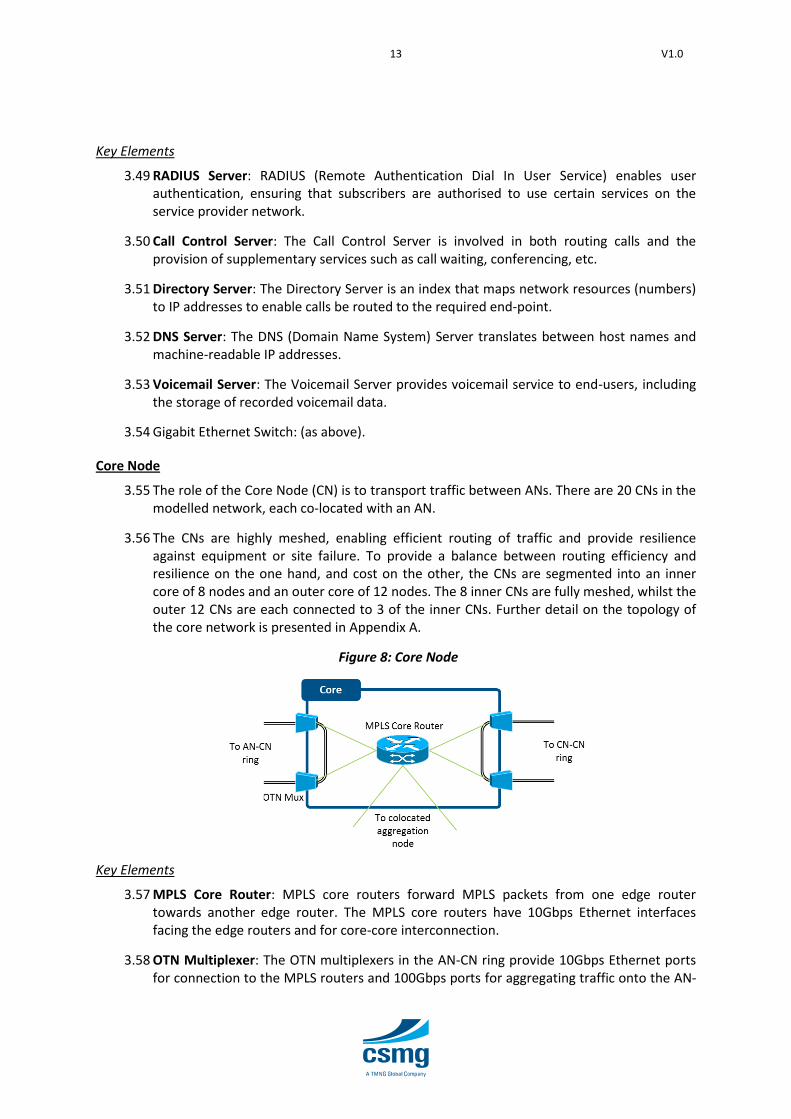
3.55 The role of the Core Node (CN) is to transport traffic between ANs. There are 20 CNs in the modelled network, each co-located with an AN.

3.56 The CNs are highly meshed, enabling efficient routing of traffic and provide resilience against equipment or site failure. To provide a balance between routing efficiency and resilience on the one hand, and cost on the other, the CNs are segmented into an inner core of 8 nodes and an outer core of 12 nodes. The 8 inner CNs are fully meshed, whilst the outer 12 CNs are each connected to 3 of the inner CNs. Further detail on the topology of the core network is presented in Appendix A.

Figure 8: Core Node

Key Elements

3.57 MPLS Core Router: MPLS core routers forward MPLS packets from one edge router towards another edge router. The MPLS core routers have 10Gbps Ethernet interfaces facing the edge routers and for core-core interconnection.

3.58 OTN Multiplexer: The OTN multiplexers in the AN-CN ring provide 10Gbps Ethernet ports for connection to the MPLS routers and 100Gbps ports for aggregating traffic onto the AN-

14 V1.0

CN ring. The OTN multiplexers in the CN-CN ring provide 10Gbps ports for connection to the MPLS routers and 100 Gbps ports for connecting traffic onto the CN – CN ring.

Example of Co-location

3.59 The figure below gives an example of a co-located core node (without interconnect or service node elements shown).

Figure 9: Co-located Core Node (Interconnect or Service Nodes not shown)

3.60 Each node in a co-located node building has one less pair of OTN equipment than when located independently, as node equipment can be cabled directly to higher-node (e.g. Super Access node to Aggregation node) equipment.

3.61 Co-located nodes exist in three combinations:

BA – SA

BA – SA – AN

BA – SA – AN (with IN and SN) – CN

Call Pathways for Modelled Services

3.62 All voice calls on the modelled network pass through either one or two ANs. The ANs house the routing capability in the network.

3.63 The table below (Figure 10) reflects the modelled media pathways for various call services on the NGN.

15 V1.0

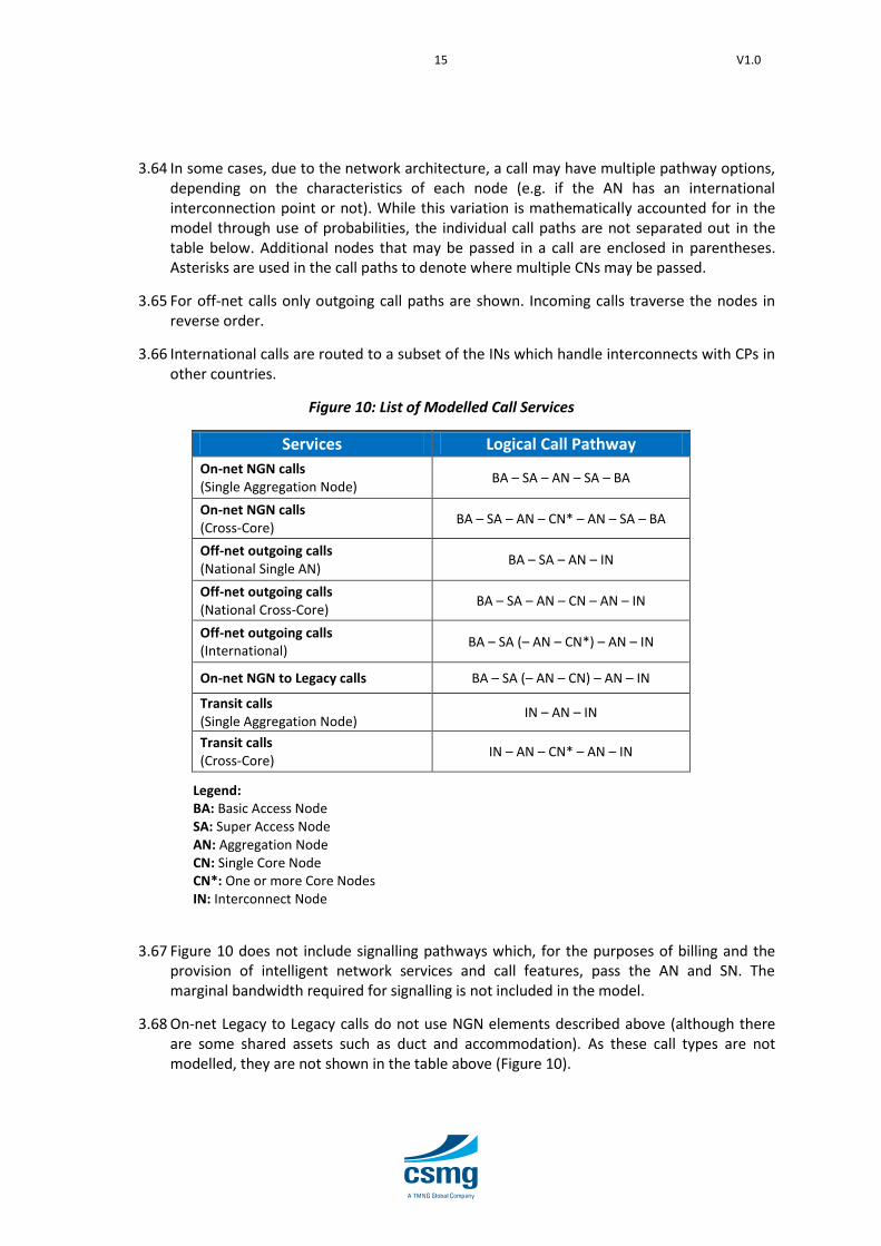
3.64 In some cases, due to the network architecture, a call may have multiple pathway options, depending on the characteristics of each node (e.g. if the AN has an international interconnection point or not). While this variation is mathematically accounted for in the model through use of probabilities, the individual call paths are not separated out in the table below. Additional nodes that may be passed in a call are enclosed in parentheses. Asterisks are used in the call paths to denote where multiple CNs may be passed.

3.65 For off-net calls only outgoing call paths are shown. Incoming calls traverse the nodes in reverse order.

3.66 International calls are routed to a subset of the INs which handle interconnects with CPs in other countries.

Figure 10: List of Modelled Call Services

Services Logical Call Pathway

On-net NGN calls (Single Aggregation Node)

BA – SA – AN – SA – BA

On-net NGN calls (Cross-Core)

BA – SA – AN – CN* – AN – SA – BA

Off-net outgoing calls (National Single AN)

BA – SA – AN – IN

Off-net outgoing calls (National Cross-Core)

BA – SA – AN – CN – AN – IN

Off-net outgoing calls (International)

BA – SA (– AN – CN*) – AN – IN

On-net NGN to Legacy calls BA – SA (– AN – CN) – AN – IN

Transit calls (Single Aggregation Node)

IN – AN – IN

Transit calls (Cross-Core)

IN – AN – CN* – AN – IN

Legend: BA: Basic Access Node SA: Super Access Node AN: Aggregation Node CN: Single Core Node CN*: One or more Core Nodes IN: Interconnect Node

3.67 Figure 10 does not include signalling pathways which, for the purposes of billing and the provision of intelligent network services and call features, pass the AN and SN. The marginal bandwidth required for signalling is not included in the model.

3.68 On-net Legacy to Legacy calls do not use NGN elements described above (although there are some shared assets such as duct and accommodation). As these call types are not modelled, they are not shown in the table above (Figure 10).

16 V1.0

4. MODEL IMPLEMENTATION AND ASSUMPTIONS

Overview of Network and Cost Modules

4.1 As outlined in the introduction to this document, CSMG has developed two modules (the Network and Cost modules) that are components within Ofcom’s NCC model.3 The Network module takes the traffic demand forecasts from the demand module and dimensions a network to carry this traffic. The Cost module calculates the capital and operating expenditure required to build the dimensioned network. The outputs from this module are used by the Economic module to calculate how costs are recovered over time and across services.

4.2 In Section 3 of this report, we identified the type of NGN that we are seeking to model. The remainder of this document will discuss how we have modelled this network and determined its costs.

Network Module

4.3 The Network module takes the network architecture, and demand inputs and dimensions the NGN to satisfy peak demand. An overview of the logic of the network module is shown in Figure 11 below.

Figure 11: Network Module Overview

3 Both modules are contained within a single Excel Workbook: 2.Network.Cost.xlsm.

17 V1.0

Call Demand

4.4 The Network module dimensions a network to carry the traffic forecast in the Demand module. The network is dimensioned to be able to carry the traffic that occurs during the busy hour. In order to use the traffic forecasts expressed in minutes for network dimensioning, we convert the traffic to busy hour megabits per second (BH Mbps).

4.5 The model considers two busy hours: a voice busy hour (for voice only traffic) and a network busy hour (that considers both voice and data traffic). The model assumes 8% of daily voice traffic occurs in the voice busy hour and 4% of daily voice traffic occurs in the network busy hour.4 As the network busy hour is driven by evening residential data demand, the model assumes that the network busy hour accounts for 8% of residential data traffic and 0.4% of business data traffic.

4.6 This draft version of the model assumes that a voice call on the modelled NGN requires 135 kbps in each direction at the IP layer, based on the use of a G.711 codec. The final version of the model will refine this figure based on CP feedback to Ofcom information requests and responses to Ofcom’s consultation. In modelling the bandwidth required for voice and data traffic, we make adjustments for Ethernet and MPLS packet headers within the network.

4.7 For call setup, the draft model assumes 500 bytes of data are transferred in each direction between the call server and the end points (MSANs, SBC or SGW). The draft model assumes there are 1.1 call attempts per call to account for unsuccessful calls. These figures will be refined in the final version of the model based on CP feedback to Ofcom information requests and responses to Ofcom’s consultation.

Categorisation of Exchanges and Network Deployment

4.8 BT currently has over 5,500 local exchanges covering the UK. These exchanges have different numbers of total lines and different proportions of business and voice lines. To account for the variation between exchanges, we define 10 different types of BA node in the model. We categorise the BA nodes based on the number of residential lines per exchange as shown in Figure 12 below.

Figure 12: Exchange Categorisation

Exchange Category Number of Residential

Premises Served Quantity of Exchanges

a 0 – 750 1,625

b 750 – 1500 1,136

c 1500 – 3000 774

d 3000 – 5000 464

e 5000 – 10000 635

f 10000 – 15000 409

g 15000 – 20000 249

h 20000 – 25000 153

i 25000 – 30000 70

j 30000+ 66

Total 5,581

4 This is because the network busy hour corresponds with the data busy hour.

18 V1.0

4.9 The higher-order nodes (i.e. SA, AN and CN) are co-located with the BA nodes. In the BT 21CN design, the selection of exchange buildings to house the higher-access nodes is a function of factors such as available space, power and redundant cable entry points plus geographic location. In line with this approach, co-location sites in the modelled network are not determined by residential line count (i.e. we do not assume the 20 sites with the largest number of residential lines are the locations of the core nodes) but rather the higher-order nodes are distributed across the BA node categories in the model.

4.10 The NGN network is built over a period of 10 years, commencing 2005/06. The NGN reaches full deployment in 2014/15 (i.e. 100% of local exchanges are NGN). By 2010/11, around 90% of lines are covered by an NGN exchange.

Figure 13: Node Migration to NGN

4.11 The network build is linked to the BA node categorization; the implementation plan assumes that for each category, the BA nodes in that category are built within a single year. We assume that all higher-order nodes (i.e. SA, AN and CN) are built during the first year.

4.12 The model assumes that a node starts to carry NGN traffic in the year after it is built. Therefore the first year in which the NGN carries traffic is 2006/07.

Dimensioning of Elements

4.13 Each network element type has up to three drivers that determine the quantity of the element required in the model:

MinDriver is the minimum number of an element that is required by the network architecture, independent of demand (i.e. the minimum quantity of a network element that would be required if there was no network traffic).

Two capacity drivers - CapacityDriver1 and CapacityDriver2 - which identify the drivers that determine how the quantity of the network elements are scaled. The capacity drivers are either (a) direct demand inputs (e.g. a function of traffic or lines); or (b) derived inputs (e.g. the number of network elements is derived from the quantity of another network element).

4.14 To simulate the capacity planning and implementation functions of a real-world operator, the model incorporates a capacity utilisation threshold. The threshold is used in conjunction with the maximum load each component can deliver to determine when capacity is expanded. Where equipment is dimensioned to cope with additional load in failure scenarios, its maximum load is adjusted to reflect this.

19 V1.0

4.15 This version of the model uses a capacity utilisation threshold of 70% for components which are dimensioned directly by demand drivers, for example the bandwidth of a network port. We will refine the capacity utilisation thresholds in the final version of the model based on CP responses to Ofcom information requests and responses to Ofcom’s consultation.

4.16 For the majority of elements, we follow a common approach to determine the required quantity for each network element in each year of the model. This approach is illustrated in Figure 14.

Figure 14: Element Dimensioning Approach

4.17 The model is also able to accommodate exceptions to the above approach. For example, in the case of network synchronisation the model always assumes three primary reference clock sources5, independent of network load or topology.

4.18 We calculate node dimensioning using the exchange categories described above. Dimensioning occurs by calculating the number of each network element required per exchange according to network and demand rules. These per-exchange values are then multiplied by the number of nodes in that exchange category, taking into account remote nodes and those co-located with SA Nodes. The model then calculates the total number of network elements required in all nodes, along with the average number per node across all exchange categories.

Calculate the Buy and Retire for Different Elements

4.19 Once the model has calculated the total number of elements required, it calculates the additional quantities required in each year given advanced planning requirements, the

5 Voice networks require accurate synchronization for correct operation. Primary reference clocks provide a

highly accurate time source for the network elements. Multiple clock sources are used for redundancy.

20 V1.0

elements purchased for additional capacity and those purchased to replace retired equipment. The model will also calculate the quantity of network elements retired.

4.20 Assets in the network model are retired at the end of their useful lives and replaced if still required. As in real-world operations, there is variation between the useful lives of different network elements in the model. We have populated the draft version of the model with a set of placeholder values for the asset lives. The asset lives in the final version of the model will be informed by CP responses to Ofcom information requests and responses to Ofcom’s consultation.

Figure 15: Asset Lifetimes by Equipment Type

Equipment Type Asset Lifetime in Draft Model (Years)

OTN 8

MSAN 5

Routers & Switches 5

Synchronisation Sources 10

Rack 10

SBC, MGW & SGW 8

Servers & Software 5

Cabling 10

4.21 The model currently assumes a planning lead time of one year. Network elements required to meet expected demand in the following year are planned, purchased and installed in the current year. This allows the NGN operator to stay ahead of expected demand on the network, and reflects typical planning and build cycles in response to, or in anticipation of, changing demand.

Cost Module

4.22 The Cost module takes its inputs from the Network module and produces total network cost estimates. The outputs from this sheet are then used as inputs in the Economic module, which implements the economic depreciation algorithm. An overview of the cost module logic is shown in Figure 16 below.

Figure 16: Cost Module Overview

21 V1.0

Element Unit Costs over Time

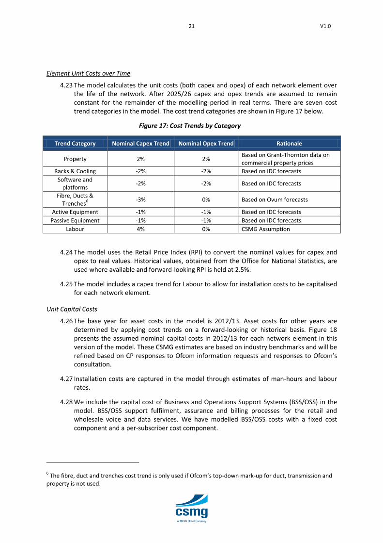
4.23 The model calculates the unit costs (both capex and opex) of each network element over the life of the network. After 2025/26 capex and opex trends are assumed to remain constant for the remainder of the modelling period in real terms. There are seven cost trend categories in the model. The cost trend categories are shown in Figure 17 below.

Figure 17: Cost Trends by Category

Trend Category Nominal Capex Trend Nominal Opex Trend Rationale

Property 2% 2% Based on Grant-Thornton data on commercial property prices

Racks & Cooling -2% -2% Based on IDC forecasts

Software and platforms

-2% -2% Based on IDC forecasts

Fibre, Ducts & Trenches

6

-3% 0% Based on Ovum forecasts

Active Equipment -1% -1% Based on IDC forecasts

Passive Equipment -1% -1% Based on IDC forecasts

Labour 4% 0% CSMG Assumption

4.24 The model uses the Retail Price Index (RPI) to convert the nominal values for capex and opex to real values. Historical values, obtained from the Office for National Statistics, are used where available and forward-looking RPI is held at 2.5%.

4.25 The model includes a capex trend for Labour to allow for installation costs to be capitalised for each network element.

Unit Capital Costs

4.26 The base year for asset costs in the model is 2012/13. Asset costs for other years are determined by applying cost trends on a forward-looking or historical basis. Figure 18 presents the assumed nominal capital costs in 2012/13 for each network element in this version of the model. These CSMG estimates are based on industry benchmarks and will be refined based on CP responses to Ofcom information requests and responses to Ofcom’s consultation.

4.27 Installation costs are captured in the model through estimates of man-hours and labour rates.

4.28 We include the capital cost of Business and Operations Support Systems (BSS/OSS) in the model. BSS/OSS support fulfilment, assurance and billing processes for the retail and wholesale voice and data services. We have modelled BSS/OSS costs with a fixed cost component and a per-subscriber cost component.

6 The fibre, duct and trenches cost trend is only used if Ofcom’s top-down mark-up for duct, transmission and

property is not used.

22 V1.0

Figure 18: Network Element Capital Costs

Asset Example Asset Name in Model 2012/13 Nominal Capex (£)

MSAN chassis BA_MSAN_Chassis 11,300

MSAN Gigabit Ethernet line card BA_MSAN_GE client card 500

MSAN voice gateway BA_MSAN_Voice gateway [incl. in line card]

OTN Gigabit Ethernet port BA_OTN_GE client port 200

OTN Gigabit Ethernet client card BA_OTN_GE client card 1,700

OTN 10Gbps Ethernet line card BA_OTN_10GE line card 4,600

OTN 10Gbps Ethernet port BA_OTN_10GE client port 900

OTN 100Gbps Ethernet client card BA_OTN_10GE client card 16,000

OTN chassis BA_OTN_Chassis 15,000

OTN rack BA_OTN_Rack 3,000

Synchronisation Source SA_Sync_SSU 30,000

Ethernet Switch Gbps port SA_Switch_GE client port 200

Ethernet Switch Gbps card SA_Switch_GE client card 9,300

Ethernet Switch 10Gbps port SA_Switch_10GE client port 1,650

Ethernet Switch 10Gbps card SA_Switch_10GE client card 11,300

Ethernet Switch chassis SA_Switch_Chassis 38,400

MPLS Edge 10Gbps port (client side) AN_Edge_10GE port (client side) 1,650

MPLS Edge 10Gbps card (client side) AN_Edge_10GE card (client side) 72,100

MPLS Edge 10Gbps port (network side)

AN_Edge_10GE port (network side) 1,650

MPLS Edge 10Gbps card (network side)

AN_Edge_10GE card (network side) 72,100

MPLS Edge chassis AN_Edge_Chassis 47,000

MPLS Core 10Gbps client port CN_MPLS_10GE client port 6,595

MPLS Core 10Gbps client card CN_MPLS_10GE client card 125,000

MPLS Core 100Gbps line card CN_MPLS_100GE line card 250,000

MPLS Core router chassis CN_Router Chassis 368,000

Primary Synchronisation Source CN_Sync_Clock 40,000

Server hardware SVC_DNS Server_Hardware 12,000

DNS server software licence SVC_DNS Server_Software licence 25,000

RADIUS server software licence SVC_RADIUS Server_Software licence 25,000

Call Server hardware SVC_Call Server_Hardware 80,000

Directory service software licence SVC_Directory Server_Software licence 25,000

Voicemail server software licence SVC_Voicemail Server_Software licence 25,000

SBC Gigabit Ethernet line card IN_Session Border Control_GE line card 25,000

SBC chassis IN_Session Border Control_Chassis 40,000

SBC software licence IN_Session Border Control_Software licence 5,000

Media Gateway Gigabit Ethernet line card

IN_Media Gateway_GE line card 19,800

Media Gateway TDM Line Card IN_Media Gateway_TDM line card 19,800

Media Gateway Chassis IN_Media Gateway_Chassis 19,200

Media Gateway Software Licence IN_Media Gateway_Software licence 20,000

OSS/BSS Systems (Fixed Costs) PAS_OSSBSS_Fixed 90,000,000

OSS/BSS Systems (Variable Cost per subscriber)

PAS_OSSBSS_PerSub 5

23 V1.0

Unit Operating Costs

4.29 Operating costs (excluding power) for each network element in the draft model are assumed to be 20% of capital costs. In the final model, we will refine this estimate based on CP responses to Ofcom information requests and responses to Ofcom’s consultation.

4.30 We caclulate the cost of power based on per network element power usage and the trended cost per kWh in the UK for industrial power supply. The network element power usage assumptions are based on standard equipment vendor guidelines.

4.31 ‘Cooling’ requirements are assumed to be proportional to per element power consumption. We assume that each kW required by network equipment produces heat that requires 0.8 kW of cooling. This estimate is benchmarked to equipment vendor guidelines.

4.32 The cost to dispose of each network element is based on the number of man hours required to dispose of that element and the cost of labour.

Calculation of Total Costs and Module Outputs

4.33 The total annual capital expenditure for each network element is calculated as the product of that year’s unit capex price and the number of network elements purchased in that year. As discussed above, the network elements purchased in each year are an output of the Network module.

4.34 The total operating expenditure is the unit opex for that year, multiplied by the number of elements in operation during that year. The annual total operating expenditure may also include the cost of decommissioning assets. We calculate the cost of decommissioning as the number of elements decommissioned in that year multiplied by the opex associated with that element’s decommissioning.

4.35 The total network capex and opex provide inputs to the economic depreciation module. In addition to the total cost outputs, the element price trends and element outputs from the cost module are also used by the economic depreciation algorithm in the Economic module. The adjusted routing factors from the Network module are also used in the Economic module to allocate the costs of network element output to network services.

24 V1.0

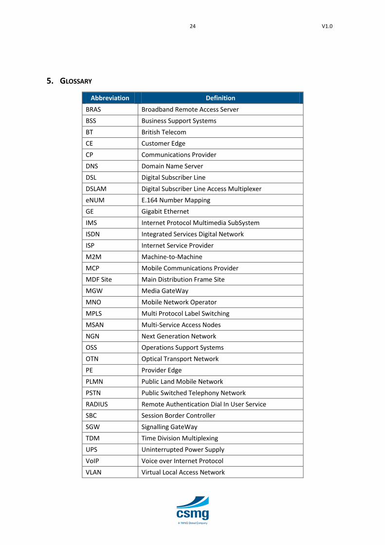
5. GLOSSARY

Abbreviation Definition

BRAS Broadband Remote Access Server

BSS Business Support Systems

BT British Telecom

CE Customer Edge

CP Communications Provider

DNS Domain Name Server

DSL Digital Subscriber Line

DSLAM Digital Subscriber Line Access Multiplexer

eNUM E.164 Number Mapping

GE Gigabit Ethernet

IMS Internet Protocol Multimedia SubSystem

ISDN Integrated Services Digital Network

ISP Internet Service Provider

M2M Machine-to-Machine

MCP Mobile Communications Provider

MDF Site Main Distribution Frame Site

MGW Media GateWay

MNO Mobile Network Operator

MPLS Multi Protocol Label Switching

MSAN Multi-Service Access Nodes

NGN Next Generation Network

OSS Operations Support Systems

OTN Optical Transport Network

PE Provider Edge

PLMN Public Land Mobile Network

PSTN Public Switched Telephony Network

RADIUS Remote Authentication Dial In User Service

SBC Session Border Controller

SGW Signalling GateWay

TDM Time Division Multiplexing

UPS Uninterrupted Power Supply

VoIP Voice over Internet Protocol

VLAN Virtual Local Access Network

25 V1.0

6. APPENDIX A: CORE NODE ARCHITECTURE

Architecture

6.1 The core network has been designed to balance inter-connectivity (which is beneficial for efficient routing and resilience) with cost.

6.2 The network core consists of 8 inner core nodes and 12 outer core nodes arranged in five physical OTN rings. One of these rings is dedicated to interconnecting the inner core nodes (the “inner ring”); the other four rings connect outer core nodes to inner core nodes (the “outer rings”).

6.3 The network model does not explicitly distinguish between inner and outer core nodes. Average values are used to determine equipment volumes across both types.

Figure 19: Core Node Architecture

Input 1: Average Links Per Core Node

6.4 At the IP/MPLS layer, the inner core nodes are fully meshed; each inner core node connects to the other seven nodes of the inner core.

6.5 The outer core nodes are not fully meshed. At the IP/MPLS layer, each outer core node connects to three of the inner core nodes.

6.6 The model uses the average number of links per core node in the network dimensioning calculations. The average number of links can be determined by summing all links and dividing by the total number of core nodes (128/20 = 6.4). This is illustrated in the table below.

26 V1.0

Figure 20: Links per Node

Node Type Number of

Nodes Ring Type

Links Per Node

Total Links Per Ring

Type

Total Links

Average Links Per

Node

Outer Core 12 Outer 3 36

128 6.4 Inner Core

nodes on two rings 4

Outer 3 12

Inner 7 28

Inner Core nodes on three rings

4 Outer 6 24

Inner 7 28

Input 2: Average Rings per Core Node

6.7 Each of the 12 outer core nodes is connected to one ring each.

6.8 Of the inner core nodes, four connect to three rings, and four connect to two rings.

6.9 The average number of rings per core node is thus, [ (12 x 1) + (4 x 2) + (4 x 3) ] / 20 = 1.6.

6.10 The network architecture requires two OTN chassis per ring (one for the “east” direction and the other for “west”). There are therefore an average of 3.2 OTN chassis per core node.

Input 3: Core Nodes Per Core Transit

6.11 Traffic on the core network can take a variety of paths depending on its source and destination. Some of these paths may involve two, three or four core nodes.

6.12 Assuming traffic is evenly distributed across the core nodes, the average number of core nodes in a path across the core can be calculated as a simple weighted average. The data for this calculation are presented in the table below.

6.13 Thus, the weighted average number of nodes passed from transit originating in the inner core is 2.7 nodes.

27 V1.0

Figure 21: Average Number of Core Nodes Passed in Transit

Source Node Quantity Destination Node Quantity Nodes Passed

Inner Node on two rings

4

Inner / same ring 7 2

Outer / same ring 3 2

Outer / other ring 9 3

Inner Node on three rings

4




Outer Node 12


Inner / other ring 5 3


Outer / adjacent ring 6 3


Input 4: Core Nodes Used per Transit to Internet Exchanges

6.14 Two core nodes link to the internet exchange. In order to minimise the average number of nodes transited to reach it from any other core node, these nodes should be on the inner ring. In addition, it is assumed that these two nodes are adjacent to each other.

6.15 The table below is used to calculate the weighted average number of core nodes transited to reach either of the two internet exchange-linked nodes.

Figure 22: Core Nodes Used per Transit to Internet Exchanges

Node Type Nodes Passed

Quantity Total Average

number of core nodes transited

Inner Core nodes

1 2 2

2.2 2 12 24

3 6 18

28 V1.0

ABOUT TMNG GLOBAL www.tmng.com

TMNG Global (NASDAQ: TMNG) is a leading provider of professional services to the converging communications industry. Its companies, TMNG, CSMG, and Cartesian, and its base of over 500 consultants, have provided strategy, management, and technical consulting, as well as products and services, to more than 1,200 communications service providers, entertainment, media, and technology companies and financial services firms worldwide. The company is headquartered in Overland Park, Kansas, with offices in Boston, London, New Jersey, and Washington, D.C.

ABOUT CSMG www.csmg-global.com

CSMG, a division of TMNG Global, is a leading strategy consultancy that focuses on the communications, digital media, and technology sectors. CSMG consultants combine a deep understanding of the global communications industry with rigorous analytic techniques to assist their clients in outmanoeuvring the competition. The organization prides itself on understanding the complex technology and financial chain that links the digital economy. CSMG serves its international client base through its offices in Boston and London.

CSMG Boston, Two Financial Center, 60 South Street, Suite 820, Boston, Massachusetts, 02111 USA

Telephone +1 617 999.1000 • Facsimile +1 617 999.1470

CSMG London, Descartes House, 8 Gate Street, London, WC2A 3HP, UK

Telephone +44 20 7643 5550 • Facsimile +44 020 7643 5555

NGN Cost Modelling - report by csmg

Documents

Transcript of NGN Cost Modelling - report by csmg