Ngl-2b031

1990 NASA/ASEE SUMMER FACULTY FELLOWSHIP PROGRAM

JOHN F. KENNEDY SPACE CENTER

UNIVERSITY OF CENTRAL FLORIDA

/

/ J

ROCKET NOISE FILTERING SYSTEM USING DIGITAL FILTERS

PREPARED BY:

ACADEMIC RANK:

UNIVERSITY AND DEPARTMENT:

NASA/KSC

DIVISION:

BRANCH:

NASA COLLEAGUE:

DATE:

CONTRACT NUMBER:

Dr. David Mauritzcn

Assistant Professor

Indiana - Purdue University - Fort WayncDepartment of Engineering

Mechanical Engineering

Special Projects

Dr. Gary Lin

August 10, 1990

University of Central FloridaNASA-NGT-60002 Supplement: 4

244

https://ntrs.nasa.gov/search.jsp?R=19910010718 2018-07-15T11:49:19+00:00Z

ACKNO_MENTS

I would like to thank my NASA colleague, Dr. Gary Lin, and his supervisor, Mr. Willis

Crumpler for the opportunity to work on this interesting project and for the very profes-

sional atmosphere they have provided. I also would like to express my gratitude to Mr. Nick

Schultz and Mr. Rudy Werlink who provided information on the current system and sample

data with which to work. The American Society of Engineering Educators (ASEE) is to be

commended for this outstanding program which provides such opportunities for professors.

The program has been smoothly administered by Professor Loren Anderson of the University

of Central Florida, and Ms. Karl Baird who has provided cordial assistance. I also appreciate

the support of my home institution, Indiana - Purdue University at Fort Wayne, the Chairman

of the Department of Engineering, Professor Muhammad Rashid, and the various members of

the administration who are helping us build our program through support of faculty

participation in programs such as this.

245

ABSTRACT

A set of digital filters is designed to filter rocket noise to various bandwidths. The filters are

designed to have constant group delay and are implemented in software on a general purpose

computer. The Parks-McClellan algorithm is used. Preliminary tests are performed to verify

the design and implementation. An analog ftlter which was previously employed is also

simulated.

,.._./

J

x,.../

246

SUMMARY

Acoustic data iscollcctcdby a fieldof sensorsduring launch. Although dataiscollectedwhich

contains validdata up to about 2 kHz, not allusersrequirefullbandwidth data. Filteringthe

data torcmov_ spectralcomponents which arc not of interestresultsin savings in storage

volume and processing time. For some applicationsitisimportant to maintain constant group

delay. A setof digitalfiltershas bccn designed and implemented which provide constantdelay,

very sharp rolloff,and largestop band attenuation.Complete processing time fora typical

fieldof sensors isIcssthan 30 hours and could readilybe reduced to lessthan 8 hours. A

program was writtentosimulate a singleanalog filterwhich had previouslybccn used for this

applicationwas writtenbut not testedbecause of time limitations.The digitaldesign

eliminatesdatamanipulation which istime consuming and i)otcntiallyerrorprone while

providing performance which ismuch superiorto analog filtering.

247

Section

I

1.1

1.2

II

2.1

2.1.1

2.1.2

2.2

2.2.1

2.2.2

2.2.3

2.2.4

2.2.5

2.2.6

2.2.7

HI

3.1

3.2

3.2.1

3.2.2

3.2.2.1

3.2.2.2

3.3

3.3.1

3.3.2

IV

TABLE OF CONTENTS

Title

INTRODUCTION

THE CURRENT ROCKET NOISE DATA PR_SING SYSTEM

DISADVANTAGES OF CURRENT SYSTEM

ANALOG AND DIGITAL FIL'IERS

THE ANALOG FILTER

The Impulse Response of the 5th Order Butterworth Filter

The Analog Filter Simulation Program

THE DIGITAL FILTER

Selection of the Digital Filter TypeLinear Phase FIR Filters

Design Algorithms

Digital Filter DesignFilter Bank Definition

Block Diagram of Filter Bank and Designations

Digital Filter Definitio

RESULTS AND DISCUSSION

PERFORMANCE OF FILTERS

DIGITAL FILTER BANK IMPLEMENTATION

The Digital Filtering Program

Initial Filter Program TestsSinusoidal Excitation Test

White Noise Excitation Test

EXF_,CIY_ON TIME AND DATA VOLUME

Reduction of Execution Time

Data Volume

CONCLUSIONS

248

-,,...j

Figure

1-1a

1-1b

2-1

2-2

2-3

2-4

2-5

LIST OF ILLUSTRATIONS

Title

Histograms of Filtered and Unfiltered Data from Sensor #1

Histograms of Filtered and Unfiltered Data from Sensor #2

Bode Plot of 5th Order Butterworth Analog Filter

Group Delay of 5th Order Butterworth Analog Filter

Topology of Digital Filter

Performance of a 1 kHz Digital Filter

Block Diagram of Digital Filter Bank

_-...._jJ

Table

3-1

3-2

3-3

LIST OF TABLES

, Title

Summary of Filter Performance

Comparison of Theoretical and Calculated Power Outputs

Power in Volts squared for the input and output files.

v

249

SECTIONI

INTRODUCTION

J

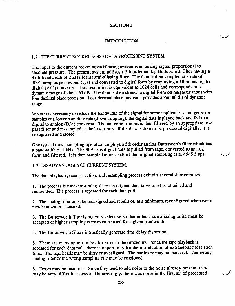
1.1 THE CURRENT ROCKET NOISE DATA PR_SING SYSTEM

The input to the current rocket noise filtering system is an analog signal proportional to

absolute pressure. The present system utilizes a 5th order analog Butterworth filter having a

3 dB bandwidth of 2 kI-Iz for its anti-aliasing filter. The data is then sampled at a rate of

9091 samples per second (sps) and converted to digital form by employing a 10 bit analog to

digital (A/D) converter. This resolution is equivalent to 1024 cells and corresponds to a

dynamic range of about 60 dB. The data is then stored in digital form on magnetic tapes with

four decimal place precision. Four decimal place precision provides about 80 dB of dynamic

range.

When it is necessary to reduce the bandwidth of the signal for some applications and generate

samples at a lower sampling rate (down sampling), the digital data is played back and fed to a

digital to analog (D/A) converter. The converter output is then filtered by an appropriate low

pass filter and re-sampled at the lower rate. If the data is then to be processed digitally, it is

re-digitized and stored.

One typical down sampling operation employs a 5th order analog Butterworth filter which has

a bandwidth of 1 kHz. The 9091 sps digital data is pulled from tape, converted to analog

form and filtered. It is then sampled at one-half of the original sampling rate, 4545.5 sps.

1.2 DISADVANTAGES OF CURRENT SYSTEM.

The data playback, reconstruction, and resampling process exhibits several shortcomings.

1. The process is time consuming since the original data tapes must be obtained and

remounted. The process is repeated for each data pull.

2. The analog filter must be redesigned and rebuilt or, at a minimum, reconfigured whenever anew bandwidth is desired.

3. The Butterworth filter is not very selective so that either more aliasing noise must be

accepted or higher sampling rates must be used for a given bandwidth.

4. The Butterworth filters intrinsically generate time delay distortion.

5. There are many opportunities for error in the procedure. Since the tape playback is

repeated for each data pull, there is opportunity for the introduction of extraneous noise each

time. The tape heads may be dirty or misaligned. The hardware may be incorrect. The wrong

analog filter or the wrong sampling rate may be employed.

6. Errors may be insidious. Since they tend to add noise to the noise already present, they

may be very difficult to detect. (Interestingly, there was noise in the first set of processed

250

1j

k,..j

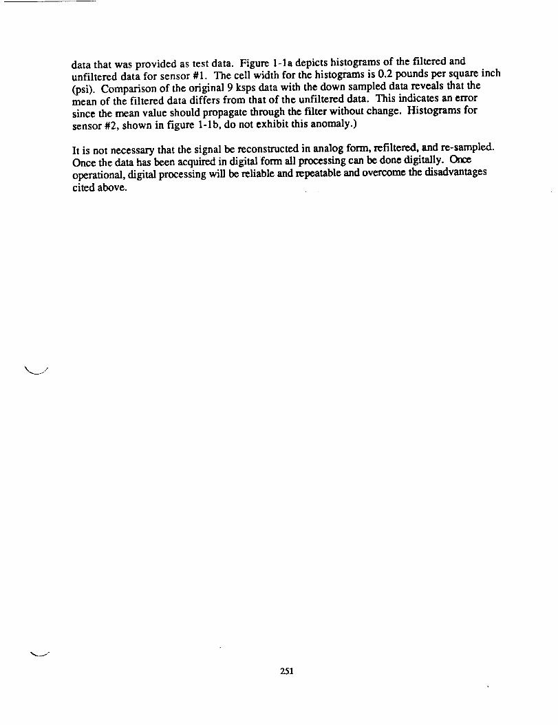
data that was provided as test data. Figure 1-1a depicts histograms of the filtered andunfiltered data for sensor #1. The cell width for the histograms is 0.2 pounds per square inch

(psi). Comparison of the original 9 ksps data with the down sampled data reveals that themean of the filtered data differs from that of the unfiltered data. This indicates an error

since the mean value should propagate through the filter without change. Histograms for

sensor #2, shown in figure 1-1b, do not exhibit this anomaly.)

It is not necessary that the signal be reconstructed in analog form, refiltered, and re-sampled.

Once the data has been acquired in digital form all processing can be done digitally. Once

operational, digital processing will be reliable and repeatable and overcome the disadvantages

cited above.

251

uJ

lZ:

0.2

0

|

' r- 7__.

CELLNO IO0

Figure l-la. Histogram of Filtered and Unfiltered Data for Sensor #1

Unfiltered Data drawn with vertical bars.

Cell width = 0.2 psi

ILl

iUl

02

0

80

[in

ri41iilI!I!1! It !

r_,';l ! I !!1i il t! ilrJ jfii!lil

....._ _fHi !! l! it fr -J t i Nt !i ! itt

r-r',,r ! I !!!i !i1!ii!_.i _- ii! I" 'l'il" 1........ ,._.:............1................_.LI.JJ..LI.I_.

C:lZLI.I'#O

' '1 , I ""'-i.

10o

Figure l-lb. Hislogram of Fillered and Unf'dtered Data for Sensor #2Urff'diered data drawn with vertical bars.

Cell width = 0.2 psi

252

v

0

-10

¢on- -4O

-50

................. r

..... I

.___.-.-...-..-.._-_

q!I

I I

! : I "L

, "r,,

%,m_

\\,

4J.D

%_

"%.

FREQUENCY. RADIANSP_ECOND

,_---;:/---_i....i I!

_ _, _ -----II

I I

i

i.

II

• L-I _L .....................

I °.

i '%,

I '_ L.

10

Figure 2-I. Bode Plot Response of 5th Order Butterworth Analog Filter

Normalized to a cbmer frequency of 1.horizontal line is -3 dB.

\ /

1

i

0

.01

i

L . , .

.1 1

FREQUENCY. RADIANS/SECOND

K

10

Figure 2-2. Group Delay of 5th Order Butierworth Filter

(for a 1 radian/second bandwidth f-alter)

253

SECTION II

ANALOG AND DIGITAL FILTERS

2.1" SIMULATION OF THE CURRENT ANALOG FILTER

It was decided to simulate the operation of the analog filter and the half rate down sampler

which is often used. This would provide continuity with previous operations, and affords the

opportunity to cross check results and detect errors. It was anticipated that this work could

be done along with the digital filter development effort within the allottext ten week interval.

The analog filter used in the 2:1 down sampling operation has a 5th order Butterworth

response, and a comer frequency of 1000 Hz. The poles of this filter lie on a circle of radius

2000*pi radians/second in the complex plane, with one pole on the negative real axis and

angular spacings between successive poles of 36 degrees. The poles are therefore at -2000*pi,

-1618*pi +/-j*1176*pi, and -618*pi 4-/-j*i902*pi. Figure 2-1 is a Bode plot of the 5th

order Butterworth response, normalized to a cut off frequency of 1 radiardsecond. The

group delay of this filter is shown in figure 2-2. The time delay is approximately constant for

low frequencies (far below the cut off frequency) but rises rapidly to a maximum in the

vicinity of the cut off frequency.

2.1.1 The Impulse Response of the 5th Order Butterworth Filter

The impulse response, h(t), for the filter will be used in the simulation of the analog filter,

and may be determined by taking the inverse Laplace transform of the transfer function of the

filter, which can be written in the form

Ao * B1 * B2

BS(s) = (1)(s + Ao) * (s 2 + A1 * s + B1) * (s 2 + A2 * s + B2)

where the name B5 was used to indicate that this is the transfer function of a 5th order

Butterworth filter. A partial fraction expansion of this transfer function may be made in theform

k...7

Co C1 * s + D1 C2 * s + D2

B5(s) - + + (2)

(s+Ao) (s 2 + A1 * s + B1) (s 2 + A2* s + B2)

The constants Co, C1, C2, D1, and D2 of this expansion may be determined by expressing the

partial fraction expansion expression as a single term, over a common denominator and

equating the coefficients of the powers of s. The resulting equations may be written inmatrix form as

254

°,__./

[C] * JU] = [K] (4)

v

where the coefficient matrix [C] is

[C] =

m

" 1 1 1 0 0

(A I +A 2) (A0+A2) (A0+A I) I I

(B I +B2+A I A2) (B 2+AOA2) (B I +AOA l) (A0+A2) (A0+AI)

(A I B2+A2B I) AOB2 A0B I (B2+AOA2) (B I +AOA I)

B I B 2 0 0 A0B 2 A0B I

(5)

and the unknown matrix [U] and constant matrix [K] are

COl

I

C1 _

[U] = C2

D1

.D2.

The unknowns are therefore

[U] = [C] -I • [K]

0

0

[K]= 0

0

k0B 1B:

Equation (2) may be inverted on a term by term basis. The inverse transform of the first

term of (2), defined as hl(t), is

hl(t) = CO * exp{-A0*t}

(6)

(7)

(8)

The second term of (2) is

Cl*s+Dl

(s 2 +A1 * s +B1)

(9)

which may be inverted to yield h2(t)

255

h2(t) = exp{-Al*t/2} * [C1 * cos(wdl*t) + CF1 * sin(wdl*t)] (10)

where

wdl - (B1 - A1^2/4)^.5

and

CF1 = (D1 - Al*Cl/2)/wdl

Since the form of the third term of (2) is the same as that of the second term, its inverse

transform, h3(t) has the same form as h2(t) except that 2 replaces 1 in the definition of the

constants C1, D1, A1, B1, wdl, and CF1. The total impulse response is the sum of yl(t),

y2(t) and y3(t).

The calculations to generate the constants and evaluate and graph h(t) have been performed in

program B5HOFT.MCD. This program stores sample values of h(t) in a disk ftle. A related

program is GB5CONST.MCD, which evaluates the constants A0, A1, A2, B1, B2, CO, C1,

C2, D1, and D2 and defines the maximum significant duration time of h(t), MAXTH and

stores this data in file B5H1K.CON for convenient use in the filtering program.

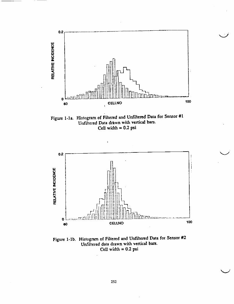
2.1.2 The Analog Filter Simulation Program

The analog filter simulation program B5A1K19.BAS simulates the 5th order Butterworth

analog filter with a 1 kHz cut off frequency that is used as an anti-aliasing filter for the 2:1

down sampling system currently in use. This program may be used either to cross check thedata produced by the traditional down sampling process or in lieu of it if so desired.

The program reads the constants which define the impulse response of the filter from file

B5H1K.CON and defines the function H(T). It then loads the data from file ZMIPHI_9.DAT

which contains zero mean pressure data which has been scaled by a factor of 100 and stored in

zero mean integer form. This data originated from sensor #1 and was acquired at 9091 sps.

(It was more efficient to work with scaled integer values of the pressure data.) The data is

read into arrays which are stored in ephemeral memory (RAM) in arrays IDH19A and IDH19B.

Two arrays were necessary because of array size limitations in Quick Basic 4.5. The filter

output is estimated by forming a numerical approximation for the convolution of the input

data with the impulse response for every multiple of the read out time interval, i.e. the

reciprocal of the output sampling rate. There were 42,976 samples in the input file. The

first 32,000 points are from array IDH19A, the rest from IDH19B. The progress of the

program is reported to the console by printing the output point number and the time for

points 1, 40, 50, 1000, and 2000. This information may then used to estimate the time to

completion. The progress information may be omitted if so desired, but the savings in

execution time will not be great. The f'flter-ou_ut is then stored in file Y'F1910KA.DAT.

This file is nominally half as large as the input file because of the 2:1 down sampling.

-...j

M_J

256

2.2 THE DIGITAL FILTER

Digital filters have the potential to outperform their analog counterparts in many respects.

Since they may be implemented as computer programs they can be of relatively high order with

essentially no increase in complexity, thus leading to steep selectivity skirts. Since no

hardware is involved, they may be readily and quickly changed. They can be designed to have

phase characteristics which are exactly linear. The group delay will then be constant for all

frequencies. They are completely stable with respect to environmental factors such as

temperature and humidity. Component aging is not a factor. Once operational, they are

reliable. Should a system fail, it will typically fail completely so that there is no uncertainty

with respect to the occurrence.

2.2.1 Selection of the Digital Filter Type

Digital filters may be classified as having either infinite impulse response (IIR) or finite impulse

response (FIR). The output of an IIR filter may extend to infinity because samples of the

output are fed back through the system. The impulse response of FIR filters must be zero

after the last non-zero input has propagated through the system. The choice of the filter type

depends upon the nature of the application and circumstance.

Although IIR filters may be unstable, FIR filters are always absolutely stable; with no feedback

there is no possibility of unbounded oscillation. Closed form design equations for IIR filters

exist for many filters, whereas there is no analogous set of design equations for FIR filters.

For similar levels of performance, a FIR filter tends to be of higher order than an IIR filter.

This leads to reduced hardware requirements and faster execution times for IIR implementa-

tions. A FIR filter may be designed to have exactly linear phase so that the time delay of the

filter can be constant for all frequencies. A more extensive comparison of the relativedifferences between FIR and IIR filters is contained in

reference 1.

Execution time is not of great consequence for our application since filtering need not be done

on a real time basis. Also, since the filter will be implemented on a general purpose computer,

hardware complexity is not a factor. The advantage of constant time delay afforded by FIR

filters is highly desirable for our application; therefore our choice is to use a FIR filter.

2.2.2 Linear Phase FIR Filters

It can be shown that a sufficient condition for linear phase response is that the unit sample

response of the system, h(n), be even symmetric about its midpoint. See, for example,reference 2.

2.2.3 Design Algorithms

Although no general closed form design algorithm exists for FIR filters, there are known

design procedures. Impulse invariance techniques are the simple, easy to employ and allow

translation of analog filter designs to digital designs, but exhibit aliasing problems and are not

usually optimum. Modifications may include the use of weighting functions (windowing) to

yield improved response. Bilinear transformation can also afford a means by which analog

filters may be translated to digital filters. These eliminate the aliasing problem associated with

257

theprevioustechnique,but themappinginvolved distorts thefrequencyscale. 0We-warping

can be employed to produce acceptable results in the case of filters having piecewise constant

transfer functions.) The design techniques cited are derivatives of analog filter designs. As

such, they lose much of the potential advantage of digital filters.

Techniques analogous to impulse invariance exist in the frequency domain. The unit sample

response of a digital filter may be obtained by taking the inverse discrete transform of samples

of the desired response in the frequency domain.

Direct approaches which do not rely on prior analog filter designs have also been developed.

Consider the design of a low pass filter having equal ripple in the pass band and in the stop

band. The parameters of interest are the order of the filter, the frequency of the upper edge

of the pass band, the frequency of the lower edge of the stop band, the ripple in the pass band

and the ripple in the stop band. These parameters are interrelated; they can not be chosenindependently. Although the problem has been formulated with many choices for the

independent variables, Parks and McClellan have developed the mathematical conditions and a

computer program which employs iterative techniques to design linear phase filters when the

order of the filter, the edge of the pass band and the edge of the stop band are given. Please

refer to references 3 and 4. The program minimizes the maximum error. The resulting filters

show nearly equal ripple throughout the band. Even high order filters may be designed

relatively quickly, although it may be desirable to repeat the design process to minimize thewidth of the transition band.

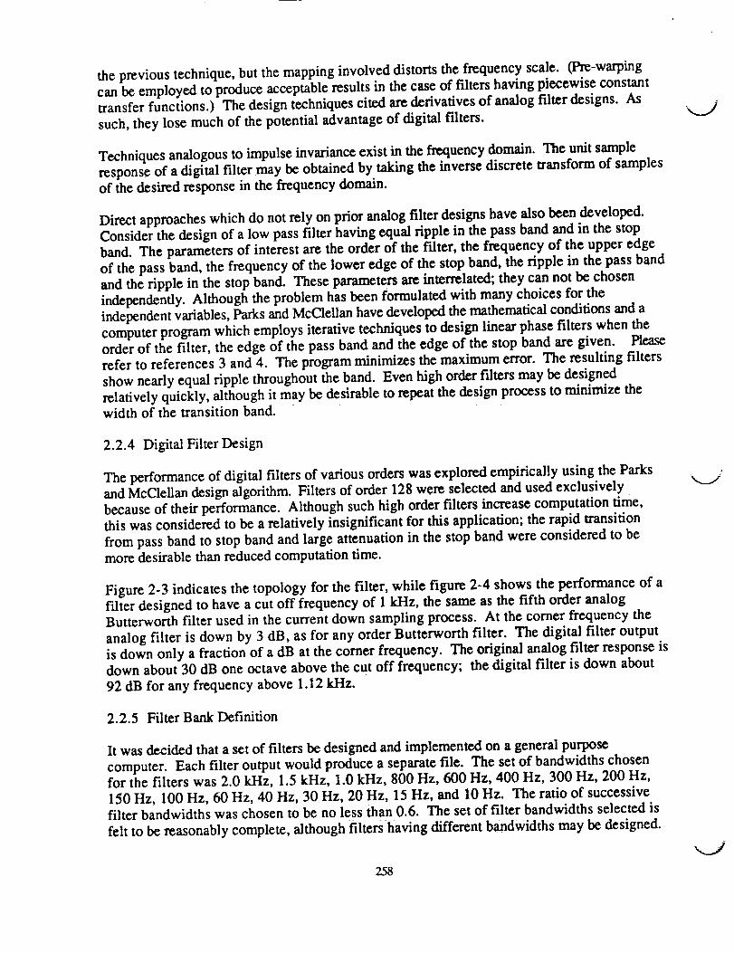
2.2.4 Digital Filter Design

The performance of digital filters of various orders was explored empirically using the Parks

and McClellan design algorithm. Filters of order 128 were selected and used exclusively

because of their performance. Although such high order filters increase computation time,

this was considered to be a relatively insignificant for this application; the rapid transition

from pass band to stop band and large attenuation in the stop band were considered to be

more desirable than reduced computation time.

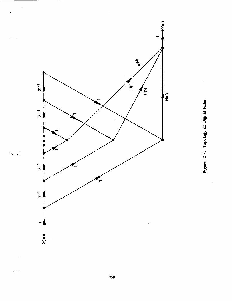
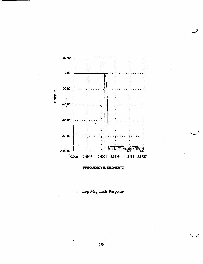
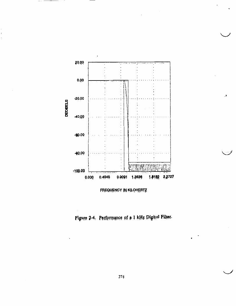
Figure 2-3 indicates the topology for the filter, while figure 2-4 shows the performance of a

filter designed to have a cut off frequency of 1 kHz, the same as the fifth order analog

Butterworth filter used in the current down sampling process. At the comer frequency the

analog filter is down by 3 dB, as for any order Butterworth filter. The digital filter output

is down only a fraction of a dB at the corner frequency. The original analog filter response is

down about 30 dB one octave above the cut off frequency; the digital filter is down about

92 dB for any frequency above 1.12 kHz.

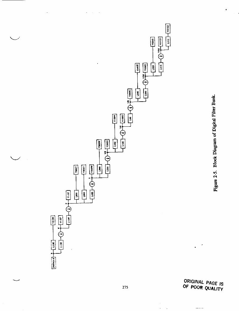
2.2.5 Filter Bank Definition

It was decided that a set of filters be designed and implemented on a general purpose

computer. Each filter output would produce a separate file. The set of bandwidths chosen

for the filters was 2.0 kHz, 1.5 kHz, 1.0 kHz, 800 Hz, 600 Hz, 400 Hz, 300 Hz, 200 Hz,

150 Hz, 100 Hz, 60 Hz, 40 Hz, 30 Hz, 20 Hz, 15 Hz, and 10Hz. The ratio of successive

filter bandwidths was chosen to be no less than 0.6. The set of filter bandwidths selected is

felt to be reasonably complete, although filters having different bandwidths may be designed.

258

_x.__j

-,...j

,7,N

"7N

"7N

"7N

6""r

.}

&

X

259

20.00

C_

0.I)0

-20.00

-40.00

-60.00

-80.00

-100.00

• ii.....................

.............. m_'_" I ....................

• o

....... i ....... i.

J

0.000 0.4545 0.9091 1.3638 1.0182 22.727

FREQUENCY IN KILOHERTZ

Figure 2-4. Performance of a 1 kHz Digital Filter.

260

Not all filters have been designed with the same sampling rate. As the spectral width of the

data is reduced by filtering to less than one-fourth the input data sampling rate, it is possible

to reduce the sampling rate by a factor of two and still meet the Nyquist sampling rate

criterion. This is done whenever possible to reduce the volume of stored data. This also

enables us to maintain the sharp selectivity skirt of the ensuing filter. Finally, the computa-

tion time is correspondingly reduced with no loss of information.

2.2.6 Block Diagram of Filter Bank and Designations

A block diagram of the f'flter bank which has been implemented is shown in figure 2-5. Low

pass filters are designated by a lead L followed by a number indicating their bandwidth.

Output files are designated by a lead Y followed by a number indicating the data bandwidth and

a letter specifying their input sampling rate. The convention used to define the sampling rateis as follows:

N - 9.091 ksps W- 1.136 ksps E -.142 ksps

F - 4.546 ksps H - .568 ksps S -.071 ksps

T -2.273 ksps Q - .284 ksps D -.036 ksps

The logicbehind these designatorsisthatthe ratesarc nominally Nine, Four, Two, Won,

Half, Quarter,one Eighth, one Sixteenth,and one thirtysecond ksps. The use of "Won"

allows us to avoid the use of O which might be confusing. The author apologizes for the

misuse of won, but the reduced probabilityof errorwarrants the potentailwrath of

grammarians. The other ratherodd usage isthe D for one thirtysecond, but occurs because

T had akcady been used to designatetwo ksps.

The input data from file ZMIPHI_9.DAT came from sensor #1 at a 9091 sps rate. (This has

been rounded to 9 ksps in the figure.) It contains data which is the integer part of 100 times

the original pressure data minus the mean value. No information has been lost by this process.

The data is filtered by the 2 kHz wide low pass filter, and data is stored in output file Y2_0N.

The same input data is also filtered by the 1.5 kHz wide low pass filter, but since this is less

than one fourth the sample frequency, it is only necessary to store alternate samples. The

two to one down sampling operation is indicated in the diagram by a circle with an arrow

pointing downward. Similar logic was used to define the rest of the filters and files.

2.2.7 Digital Filter Definition

The sixteen filters cited in the previous section may be defined by citing their unit sample

responses. The array defining the unit sample responses of the filters is in disk fde available

upon request.

261

I ,,.._j

-,,,..j

262ORIGINAL PAGE IS

OF POOR QUALITY

SECTION HI

RESULTS AND DISCUSSION

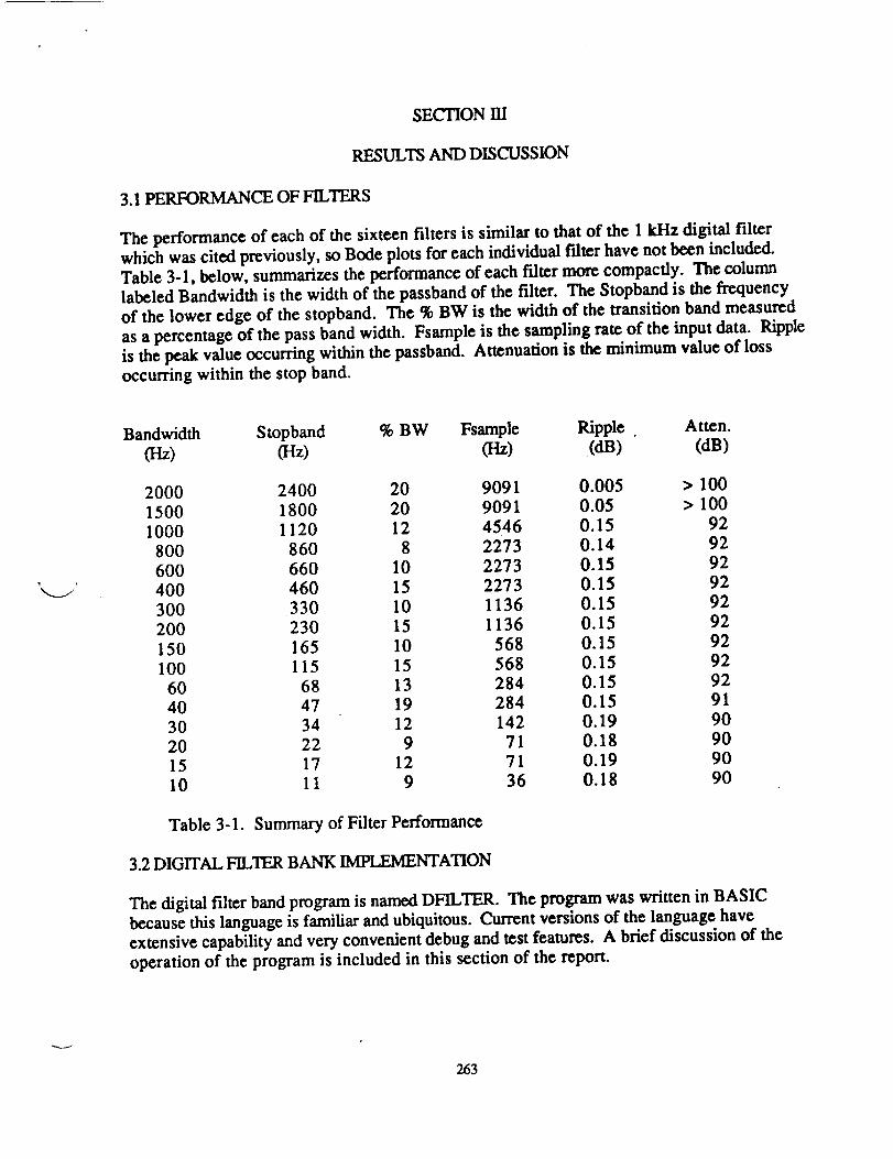
3.1 PERFORMANCE OF FILTERS

The performance of each of the sixteenfiltersissimilarto thatof the 1 kHz digitalfilter

which was citedpreviously,so Bode plotsforeach individualfilterhave not been included.

Table 3-I,below, summarizes the performance of each faltermore compactly. The column

labeledBandwidth isthe width of the passband of the filter.The Stopband isthe frequency

of the lower edge of the stopband. The % BW isthe width of the transitionband measured

as a percentage of the pass band width. Fsample isthe sampling rateof the input data. Ripplc

isthe peak value occurring withinthepassband. Attenuationisthe minimum value of loss

occurring within the stop band.

Bandwidth Stopband % BW Fsample Ripple. Atten.

(Hz) (Hz) (Hz) (dB) (dB)

2000 2400 20 9091 0.005 > 100

1500 1800 20 9091 0.05 > 100

1000 1120 12 4546 0.15 92

800 860 8 2273 0.14 92

600 660 10 2273 0.15 92

400 460 15 2273 0.15 92

300 330 10 1136 0.15 92

200 230 15 1136 0.15 92

150 165 I0 568 0.15 92

100 115 15 568 0.15 92

60 68 13 284 0.15 92

40 47 19 284 0.15 91

30 34 12 142 0.19 90

20 22 9 71 0.18 90

15 17 12 71 0.19 90

I0 11 9 36 0.18 90

Table 3-1. Summary of Filter Performance

3.2 DIGITAL FILTER BANK IMPLEMENTATION

The digital filter band program is nan_ DFILTER. The program was written in BASIC

because this language is familiar and ubiquitous. Current versions of the language have

extensive capability and very convenient debug and test features. A brief discussion of the

operation of the program is included in this section of the report.

263

3.2.1 The Digital Filtering Program

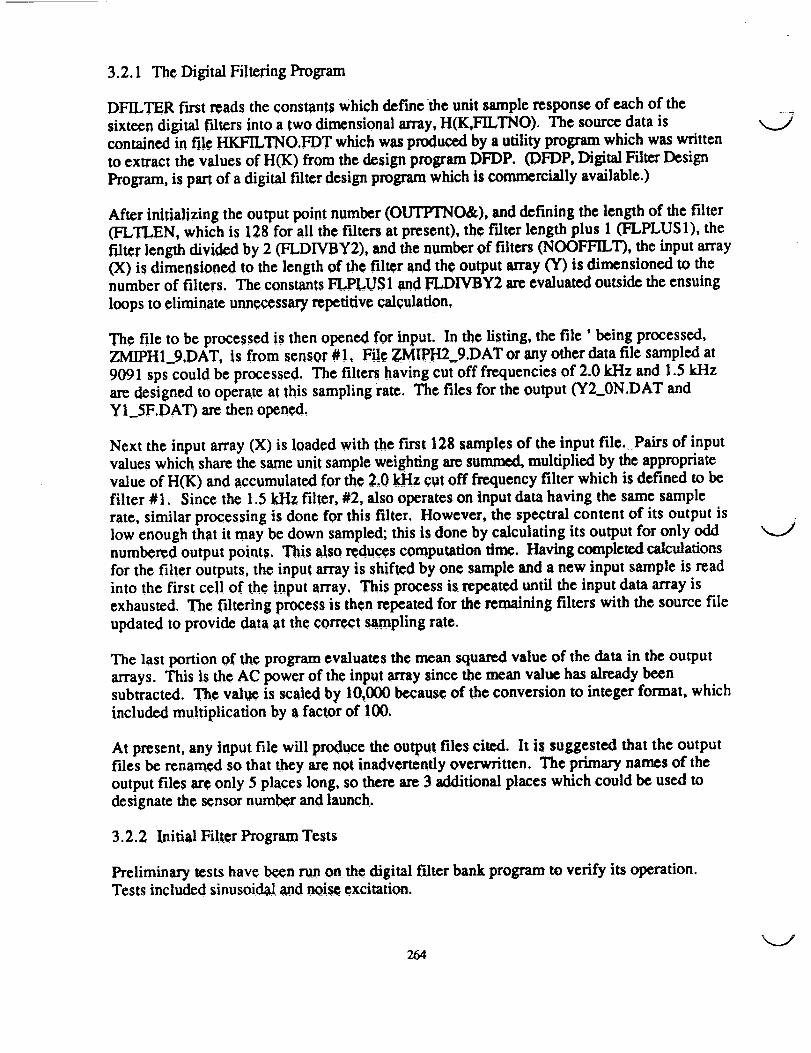
DF!LTER fu'st reads the constants which define the unit sample response of each of thesixteen digital filters into a two dimensional array, H(K,FILTNO). The source data iscontained in file HKFILTNO.FDT which was produced by a utility program which was writtento extract the values of H(K) from the design program DFDP. (DFDP, Digital Filter Design

Program, is pan of a digital filter design program which is commercially available.)

After initializing the output point number (OUTPTNO&), and defining the length of the filter(FLTLEN, which is 128 for all the filters at present), the f'flter length plus 1 (FLPLUS1), the

filter length divided by 2 (FLDIVBY2), and the number of filters (NOOFFILT), the input array(X) is dimensioned to the length of the filter and the output array 0f) is dimensioned to thenumber of filters. The constants FLPLUS 1 and _DWBY2 are evaluated outside the ensuing

loops to eliminate unn_essary repetitive calculation,

The file to be processed is then opened for input. In the listing, the file ' being processed,ZMIPHI_9,DAT, is from sensor #1, File ZM!PH2_9.DAT or any other data file sampled at

9091 sps could be processed. The filters having cut off frequencies of 2.0 kHz and 1.5 kHzare designed to operate at this sampling rate. The files for the output Of 2_0N.DAT andYI_SF.DAT) are then opened.

Next the input array (X) is loaded with the f'mst 128 samples of the input file. Pairs of inputvalues which share the same unit sample weighting are summed, multiplied by the appropriatevalue of H(K) and accumulated for the 2.0 kHz cut off frequency filter which is defined to befilter #1. Since the 1.5 kHz filter, #2, also operates on input data having the same sample

rate, similar processing is done for this filter. However, the spectral content of its output islow enough that it may be down sampled; this is done by calculating its output for only oddnumbered output points. This also reduces computation time. Having completed calculationsfor the filter outputs, the input array is shifted by one sample and a new input sample is readinto the first cell of the input array, This process is repeated until the input data array isexhausted. The filtering process is then repeated for the remaining filters with the source file

updated to provide data at the correct sampling rate.

The last portion of the program evaluates the mean squared value of the data in the outputarrays. This is the AC power of the input array since the mean value has already beensubtracted. The value is scaled by 10,000 because of the conversion to integer format, whichincluded multiplication by a factor of 100.

At present, any input file will prod_e the output files cited. It is suggested that the outputfiles _ renamed so that they are not inadvertently overwritten. The primary names of the

output files are only 5 places long, so there are 3 additional places which could be used to

designate the _nsor number and launch.

3.2.2 Initial FiRer Program Tests

Preliminary tests have been run on the digital filter bank program to verify its operation.Tests included sinusoidal and nois_ excitation.

264

J

---..._

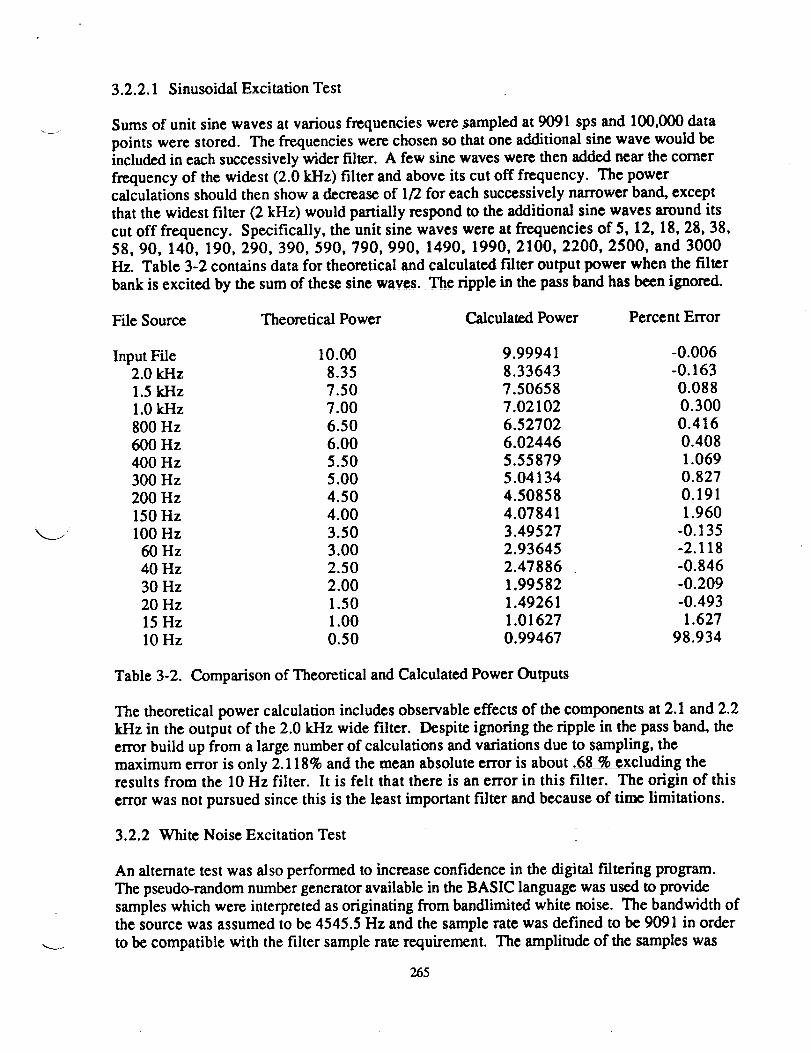
3.2.2.1 Sinusoidal Excitation Test

Sums of unit sine waves at various frequencies were sampled at 9091 sps and 100,000 data

points were stored. The frequencies were chosen so that one additional sine wave would be

included in each successively wider filter. A few sine waves were then added near the corner

frequency of the widest (2.0 kHz) filter and above its cut off frequency. The powercalculations should then show a decrease of 1/2 for each successively narrower band, except

that the widest filter (2 kHz) would partially respond to the additional sine waves around its

cut off frequency. Specifically, the unit sine waves were at frequencies of 5, 12, 18, 28, 38,58, 90, 140, 190, 290, 390, 590, 790, 990, 1490, 1990, 2100, 2200, 2500, and 3000

Hz. Table 3-2 contains data for theoretical and calculated filter output power when the filter

bank is excited by the sum of these sine waves. The ripple in the pass band has been ignored.

File Source Theoretical Power Calculated Power Percent Error

Input File 10.00 9.99941 -0.0062.0 kI-Iz 8.35 8.33643 -0.163

1.5 kHz 7.50 7.50658 0.088

1.0 kHz 7.00 7.02102 0.300

800 Hz 6.50 6.52702 0.416

600 Hz 6.00 6.02446 0.408

400 Hz 5.50 5.55879 1.069

300 Hz 5.00 5.04134 0.827

200 Hz 4.50 4.50858 0.191

150 Hz 4.00 4.07841 1.960

100 Hz 3.50 3.49527 -0.135

60 Hz 3.00 2.93645 -2.118

40 Hz 2.50 2.47886 _ -0.846

30 Hz 2.00 1.99582 -0.209

20 Hz 1.50 1.49261 -0.493

15 Hz 1.00 1.01627 1.627

10 Hz 0.50 0.99467 98.934

Table 3-2. Comparison of Theoretical and Calculated Power Outputs

The theoretical power calculation includes observable effects of the components at 2.1 and 2.2

kHz in the output of the 2.0 kHz wide filter. Despite ignoring the ripple in the pass band, the

error build up from a large number of calculations and variations due to sampling, the

maximum error is only 2.118% and the mean absolute error is about .68 % excluding the

results from the 10 Hz filter. It is felt that there is an error in this filter. The origin of this

error was not pursued since this is the least important filter and because of time limitations.

3.2.2 White Noise Excitation Test

An alternate test was also performed to increase confidence in the digital filtering program.

The pseudo-random number generator available in the BASIC language was used to provide

samples which were interpreted as originating from bandlimited white noise. The bandwidth of

the source was assumed to be 4545.5 Hz and the sample rate was defined to be 9091 in order

to be compatible with the filter sample rate requirement. The amplitude of the samples was

265

scaled to provide a noise power spectral density of 1 volt squared per Hz, and 100,000

samples were generated and stored in a file.

The file of noise samples was then fed to the filter bank program as input data. The power of

the data in the input fi!e and in the data of each output file were estimated. The power in the

output files should be proportional to the equivalent noise bandwidth. Since the spectral

density was scaled to unity, we expect the output power to be numerically equal to the

equivalent noise bandwidth of the filter in a statistical sense. The equivalent noise bandwidth

of the filters was not calculated, but may reasonably expected to be Limited to a value greater

than the pass band width but less than the e<!ge of the stop band, These Limits are only valid

in a statistical sense, and only ont_ random noise sample file was run, The number of samples

in outputs of the wider filters is quite large, and the variability of the power should be

relatively small. Table 3-3 is a tabulation of the power in the input file, the power in each of

filter outputs, and the limits cited.

File Power Power Limi+'ts

Name Estimated Lower Upper

INPUT 4553.666 4546 4546

Y2_0NWN 2126.869 2000 2400

YI_5FWN 1583,643 1500 !800

YI_0TWN 1032.652 1000 1120

Y800TWN 820.728 800 860

Y600TWN 623.858 600 660

Y400WWN 420.640 400 460

Y300WWN 316.196 300 330

y200HWN 214,496 200 230

Y150HWN 156.262 !50 165

Y100QWN 106.328 100 ! !5

Y060EWN 61,536 60 68

Y040EWN 40.286 40 47

Y030SWN 31.766 30 34

Y020SWN !9.942 20 22

Y015DWN !4;566 15 !7

Y010DWN 13.660 10 11

Table 3-3, Power in Volts squared for the input and output files.

Agreement is excellent for nearly all the fdes, although the power in the filters having

bandwidths of 20 Hz and 15 Hz is very slightly low, this may be a consequence of statistical

variation and the relatively small sample size available at these low frequencies. The only

questionable result is once again that from the 10 Hz filter. Its output appears to be undulyhigh. This result again makes this filter implementation suspect.

3.3 _CUTION TIME AND DATA VOLUME

A complete run, including filter OUtpUt power calculations in BASIC, for the white noise test

sample, which consisted of 100,000 points of data, took less than three hours to complete

266

on a computer having a 80386 CPU and a 80387 co-processor chip running at a speed of 16

MHz. This volume of data is equivalent to the output of one sensor for 11 seconds, so the

execution time is about .27 hours/sensor-second. A set of 10 sensors collecting data for 11

seconds each would lead to a total processing time of about 30 hours under the conditions

cited. Since this is a non-recurrent operation for a given launch, the current execution time

may be acceptable.

3.3.1 Reduction of Execution Time

Run time could be reduced by using a faster machine, say a 33 MHz system, thus speeding

execution by a factor of 2. It would be possible to use one of the new 80486 systems,

which are reputed to be 2 to 4 times faster than the 80386 machines. The program could

also be run on a mini, mainframe, or other faster machines. A compiled language program

would also execute more rapidly. Additionally, the program could be modified to reduce

computation time. For example, the shift register operation, which mimics a hardware

implemented shift register could be replaced by a functionally equivalent system in which the

data is loaded into an array in RAM and accessed by pointers. This implementation would

most likely be quicker. It is also possible that transform techniques may be faster.

3.3.2 Data Volume

The data volume may be reduced with no loss of information by storing only the sampling

interval and a sequential set of pressure samples. The pressure samples may be stored in

integer format rather than floating point. Data compression techniques, which are currently in

use, should be continued for archival purposes.

267

SECTION4

OONCLUSIONS

A filter bank of !5 digital filters has been designed and implemented in software for this

project and appears to be functioning correctly, although additional verk¢lcation work would

further increase confidence.

The all-digital filtering program is far more versatile than the previous system. It is much

more extensive.

Should different applications require different bandwidths, a new set of digital filters could be

quickly, easily, and inexpensively designed and implemented.

The performance attained by the digital filters far exceeds that of their analog predecessorboth in roll off rate and attenuation, Aliasing errors are correspondingly reduced, assuming

the adequacy of the analog anti-aliasing filter.

The time delay for the digital filters is constant for all frequencies, so there is no distortion

caused by relative time shifts between the spectral components of a signal.

The time to process 11 seconds of data from 10 sensors may be filtered and the power in the

filter outputs calculated in less than 30 hours. The processing time could be easily reduced toless than 8 hours.

Once operational, the digital filtering system is reliable and error free. No analog signal

reconstruction, filtering and resampling operations are necessary, thus eliminating many

opportunities for error.

The volume of data could be further reduced and subsequent processing time decreased if the

sampling rate were made close to the Nyquist rate for each filter bandwidth. This would

require non-integer changes in the sampling frequency. It is possible, through a process of

upsampling and down sampling, to produce sampling rates which related by any rationalnumber.

The analog filter simulation was written but not verified due to time limitations. It was a

secondary goal, intended to provide cross comparison and verification of the current

processing system. It was therefore given lower priority than the digital effort.

,,..j

References

1. L.R. Rabiner, J. F. Kaiser, O. Herrmann, and M. T. Dolan, "Some Comparisons between

FIR and IIR Digital Filters," Bell System Technical Journal, Volume 53, Number 2, February,

1974, pages 305 - 331.

2. Alan V. Oppenheim and Ronald W. Schafer, "Digital Signal Processing," Prentice-Hall, 1975.

3. T.W. Parks and J. H. McClellan, "Chebyshev Approximation for Non-recursive DigitalFilters with Linear Phase," IEEE Transactions Circuit Theory, Volume CT-19, March, 1972,

pages 189- 194.

4. T.W. Parks and J. H. McClellan, "A Program for the Design of Linear Phase Finite Impulse

Response Filters," IEEE Transactions Audio Electroacoustics, Volume AU-20, Number 3,

August, 1972, pages 195- 199.

269

20.00

m

r_

0.00

-20.00I

,,40.1)0

-60.00

-80.00

-100.00

• .. ..._ • .o • • .. . ° .° . . °

\

I

II....... i o . o... o _ ....... I . .....° i ..... . o

,i

IfULqI.H,_,,[!H.Ii ,t_._.!.t ,_!.L_;.',I ,'lD,_I

0.000 0.4545 0.9091 1,3636 1.8182 2.2727

FREQUENCY IN KILOHERTZ

Log Magnitude Response

:.._j

270

0

0.2 1.................................................".............. -- I

1

• I

_: .'_"!/_,_ / _,i _,i i __ • _,_ ___ i_j _.:_.._..u_...... 100

60

Fip._tc 1.1a. I4istograrn o_ Filtered and Onftltcrcd Data for ScnSO_ #1Unf_ItcrcdData drawn with x,c_icalbarS,

Cellwidth= 0.2psi

O:2

C2

1: 1

1I,

ii: !

,i'!i !!! '" i

r.-_,.ig!i !_ _! i, _ii_i_ :_

_i.,i_i_ .._.'-n

..... • t_ '' ......

0 "_ "_............................. CELLNO

6O

Figure t-lb." Histogram o_ Filtered and Llni'tlte_ed Data _o_ Sensor #2 -unfiltereddata drawn with verticalbarS.

Cell width _ 0.2 psi

ORIGINAL PAGE ISOF POOR QUALITY

271

0

.t0

0.t

...........................................................i..............................i.........i........i

t

...................................... ,.......I--_ --.,

, ' !

I i i

J!

! !

•.T,::-:q_:iTi......................., ........

"_*i .......... i ............

I

_i:cyLill_N_,Y,IIAi:IIANI!t/gBI_I_D

-.Zt ................................ I'""" I.....

I

........ "_ i_*---.tl _-.-tl .....

!rT-1.....1o

-.._2

Figure _-|. ]_ode Plot Re_ot_se of 5th Order Butterworth Analog FilterHormalized to _tcorner frequen_ of 1.

horizor_tal llne is -3 dB.

i

o

0

t i -7 I]t1!t ! , f,.............................................................Hiii.........................t............!........t...............................................................t-.li-iJ.............l........I........t....¸-i..............................................!,i t .........fi-t-,,__..____. i ...........T!.....................i.7

....... -;-i-T-FI.................I....1_....

I

' It! 1;o_ .i

_]i

i

i':']

i'_ <,,,]

I

i

i

................t'l.....!1_ I i

i l % I '! i _, t

I I _..,

"!l "-.....,L.L...............................-_':::

1

Pigul_ _-_.Orolip Delay of _lth Order ituti6_lsiih Filter(t'or li i radiardsecond bandwidth Fiber)

8

-T"

*v,4

¢_

0

&

oel

X

273

!

;_O.Qq

o.oo

-20.00

-40:QO

-_.0_

.... i . ._ .... , .......

rl i ....................i i ii; ....... ...... " .I, . _.... ...... i ......

i i i i

.b

F_._.,I_HPY IN Kll-OHF.W['_

274

v

U 9

1I

275

"d

°_,,I

¢.q

ORIGINAL PAGE IS

OF POOR QUALITY