Newton’s Laws of Motion

Claude A Pruneau

Physics and Astronomy

Wayne State University

PHY 5200 Mechanical Phenomena

Click to edit Master title style

Click to edit Master subtitle style

1

Projectile Motion

PHY 5200 Mechanical Phenomena

Claude A PruneauPhysics and Astronomy DepartmentWayne State UniversityDec 2005.

ContentContent

• Projectile Motion– Air Resistance– Linear Air Resistance– Trajectory and Range in a Linear Medium– Quadratic Air Resistance

• Charge Particle Motion– Motion of a Charged Particle in a Uniform Field– Complex Exponentials– Motion in a Magnetic Field

Description of Motion with F=ma

• F=ma, as a law of Nature applies to a very wide range of problems whose solution vary greatly depending on the type of force involved.

• Forces can be categorized as being “fundamental” or “effective” forces.

• Forces can also be categorized according to the degree of difficulty inherent in solving the 2nd order differential equation F = m a.– Function of position only– Function of speed, or velocity– Separable and non-separable forces

• In this Chapter– Separable forces which depend on position and velocity.– Non separable forces.

Air Resistance

• Air Resistance is neglected in introductory treatment of projectile motion.

• Air Resistance is however often non-negligible and must be accounted for to properly describe the trajectories of projectiles. – While the effect of air resistance may be very small in some

cases, it can be rather important and complicated e.g. motion of a golf ball.

• One also need a way/technique to determine whether air resistance is important in any given situation.

Air Resistance - Basic Facts

• Air resistance is known under different names– Drag– Retardation Force– Resistive Force

• Basic Facts and Characteristics– Not a fundamental force…– Friction force resulting from different atomic phenomena– Depends on the velocity relative to the embedding fluid.– Direction of the force opposite to the velocity (typically).

• True for spherical objects, a good and sufficient approximation for many other objects.

• Not a good approximation for motion of a wing (airplane) - additional force involved called “lift”.

– Here, we will only consider cases where the force is anti-parallel to the velocity - no sideways force.

Air Resistance - Drag Force

• Consider retardation force strictly anti-parallel to the velocity.

• Where

f(v) is the magnitude of the force.

• Measurements reveal f(v) is complicated - especially near the speed of sound…

• At low speed, one can write as a good approximation:

rw =m

rg

rf =−f (v)v̂

v̂

rf =−f (v)v̂

v̂ =

rv r

v

f (v)=bv+ cv2 = flin + fquad

Air Resistance - Definitions

f (v)=bv+ cv2 = flin + fquad

flin ≡bv Viscous drag• Proportional to viscosity of the medium

and linear size of object.

Inertial• Must accelerate mass of air which is in

constant collision. • Proportional to density of the medium

and cross section of object.

fquad ≡cv2

For a spherical projectile (e.g. canon ball, baseball, drop of rain):

b =βD

c =γD2Where D is the diameter of the sphereβand γ depend on the nature of the mediumAt STP in air:

β =1.6 ×10−4Ngs / m2

γ = 0.25Ngs / m4

Air Resistance - Linear or Quadratic

• Often, either of the linear or quadratic terms can be neglected.

• To determine whether this happens in a specific problem, consider

• Example: Baseball and Liquid Drops

• A baseball has a diameter of D = 7 cm, and travel at speed of order v=5 m/s.

• A drop of rain has D = 1 mm and v=0.6 m/s

• Millikan Oil Drop Experiments, D=1.5 mm and v=5x10-5 m/s.

fquadflin

=cv2

bv=γDβ

v= 1.6 ×103 sm2( )Dv

= 1: linear case

? 1: quadratic case

⎧

⎨⎪

⎩⎪

fquadflin

≈600

fquadflin

≈1

fquadflin

≈10−7

rf =−cv2v̂

Neither term can be neglected.

rf =−b

rv

Air Resistance - Reynolds Number

• The linear term drag is proportional to the viscosity, • The quadratic term is related to the density of the

fluid, .• One finds

fquadflin

: R ≡Dv Reynolds Number

Case 1: Linear Air Resistance

• Consider the motion of projectile for which one can neglect the quadratic drag term.

• From the 2nd law of Newton:

• Independent of position, thus:

• Furthermore, it is separable in coordinates (x,y,z).

• By contrast, for f(v)~v2, one gets coupled y vs x motion

mr&&r =

rF =m

rg−b

rv

rw =m

rg

rf =−b

rv

v̂

mr&v =m

rg−b

rv A 1st order differential equation

y

x

m&vx =−bvx

m&vy =mg−bvy

Two separate differential equationsUncoupled.

rf =−cv2v̂=−c vx

2 + vy2 rv

m&vx =−c vx2 + vy

2vx

m&vy =mg−c vx2 + vy

2vy

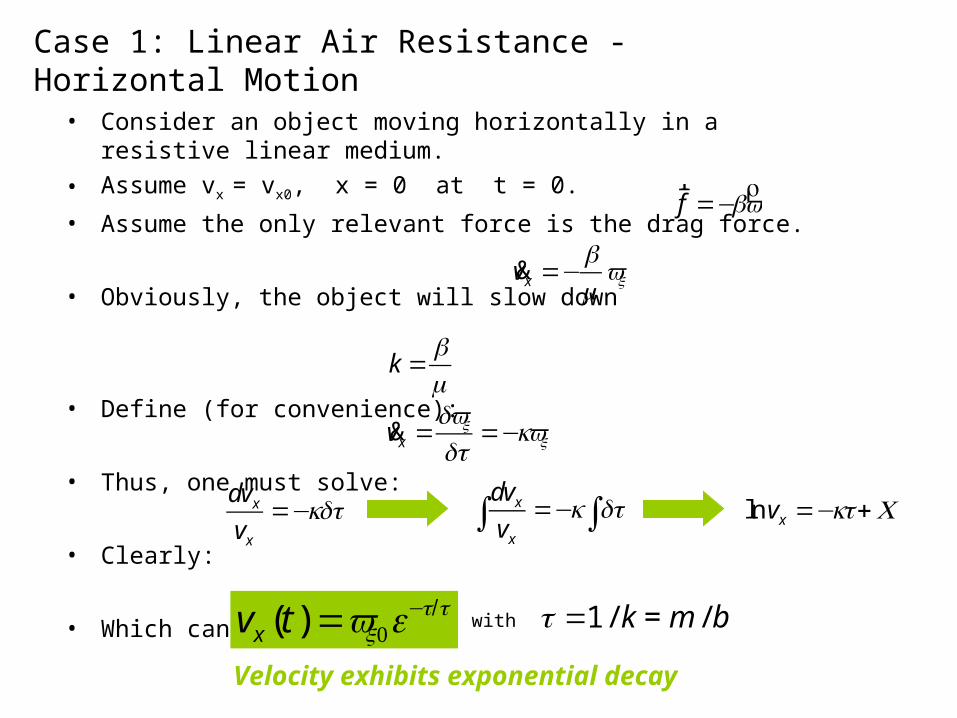
Case 1: Linear Air Resistance - Horizontal Motion

• Consider an object moving horizontally in a resistive linear medium.

• Assume vx = vx0, x = 0 at t = 0.

• Assume the only relevant force is the drag force.

• Obviously, the object will slow down

• Define (for convenience):

• Thus, one must solve:

• Clearly:

• Which can be re-written:

rf =−b

rv

&vx =−

bm

vx

k =bm

&vx =

dvx

dt=−kvx

dvxvx

=−kdtdvxvx

∫ =−k dt∫ lnvx =−kt+C

vx (t)=vx0e−t/τ

with τ =1 / k = m / b

Velocity exhibits exponential decay

Case 1: Linear Air Resistance - Horizontal Motion (cont’d)

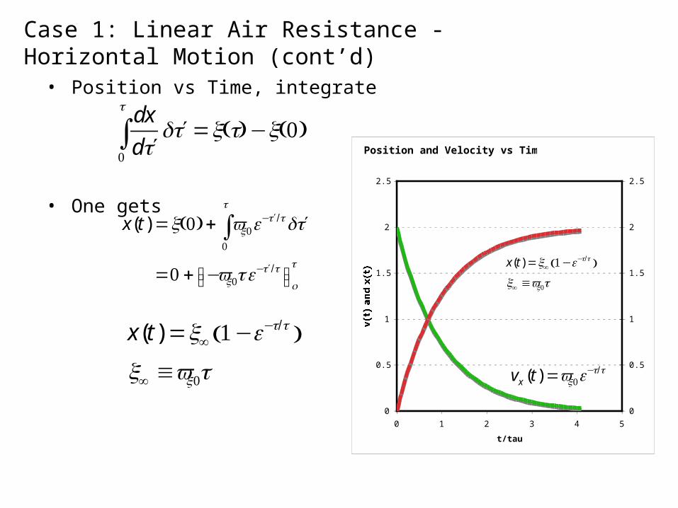
• Position vs Time, integrate

• One gets

dx

d ′td ′t

0

t

∫ =x(t)−x(0)

x(t)=x(0) + vx0e− ′t /τd ′t

0

t

∫

=0 + −vx0τe− ′t /τ⎡⎣ ⎤⎦o

t

x(t)=x∞ 1−e−t/τ( )

x∞ ≡vx0τ

Position and Velocity vs Time

0

0.5

1

1.5

2

2.5

0 1 2 3 4 5

t/tau

v(t) and x(t)

0

0.5

1

1.5

2

2.5

x(t)=x∞ 1−e−t/τ( )

x∞ ≡vx0τ

vx (t)=vx0e−t/τ

Vertical Motion with Linear Drag

• Consider motion of an object thrown vertically downward and subject to gravity and linear air resistance.

• Gravity accelerates the object down, the speed increases until the point when the retardation force becomes equal in magnitude to gravity. One then has terminal speed.

m&vy =mg−bvy

rw =m

rg

rf =−b

rv

v̂y

x

0 =mg−bvy vter =vy(a=0) =mgb

Note dependence on mass and linear drag coefficient b.Implies terminal speed is different for different objects.

Equation of vertical motion for linear drag

• The equation of vertical motion is determined by

• Given the definition of the terminal speed,

• One can write instead

• Or in terms of differentials

• Separate variables

• Change variable:

m&vy =mg−bvy

vter =mgb

m&vy =−b vy −vterm( )

mdvy =−b vy −vterm( )dt

dvyvy −vterm

=−bdtm

u =vy −vterm

du=dvy

du

u=−

bdtm

=−kdt

k =bmwhere

Equation of vertical motion for linear drag (cont’d)

• So we have …

• Integrate

• Or…

• Remember

• So, we get

• Now apply initial conditions: when t = 0, vy = vy0

• This implies

• The velocity as a function of time is thus given by

du

u=−

bdtm

=−kdt

du

u∫ =−k dt∫ lnu =−kt+C

u =vy −vterm

u =Ae−kt

vy −vter =Ae−t/τwith τ =1 / k = m / b

vy0 −vter =Ae−0/τ =A

vy =vter + vy0 −vter( )e−t/τ

vy =vy0e−t/τ + vter 1−e−t/τ( )

Equation of vertical motion for linear drag (cont’d)

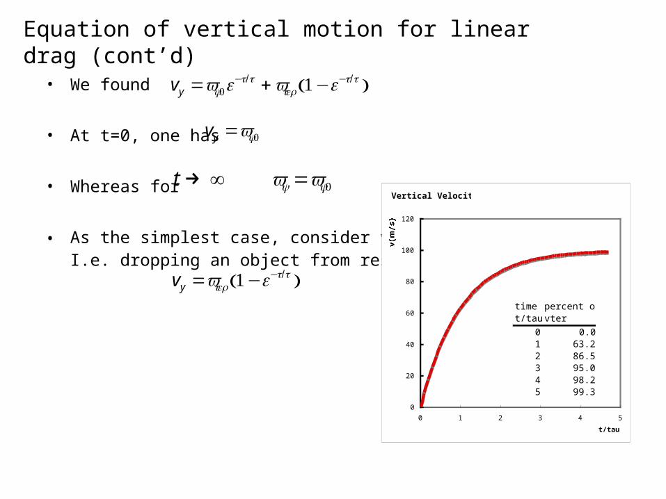
• We found

• At t=0, one has

• Whereas for

• As the simplest case, consider vy0=0,I.e. dropping an object from rest.

vy =vy0e−t/τ + vter 1−e−t/τ( )

vy =vy0

t → ∞ vy =vy0

vy =vter 1−e−t/τ( )

Vertical Velocity

0

20

40

60

80

100

120

0 1 2 3 4 5

t/tau

v(m/s)

time t/tau

percent of vter

0 0.01 63.22 86.53 95.04 98.25 99.3

Equation of vertical motion for linear drag (cont’d)

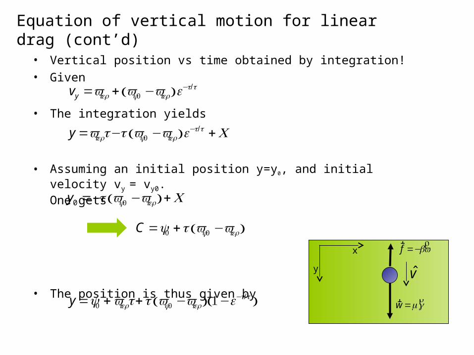
• Vertical position vs time obtained by integration!

• Given

• The integration yields

• Assuming an initial position y=y0, and initial velocity vy = vy0.One gets

• The position is thus given by

vy =vter + vy0 −vter( )e−t/τ

y =vtert−τ vy0 −vter( )e−t/τ +C

y0 =−τ vy0 −vter( ) +C

C =y0 +τ vy0 −vter( )

y =y0 + vtert+τ vy0 −vter( ) 1−e−t/τ( ) rw =m

rg

rf =−b

rv

v̂y

x

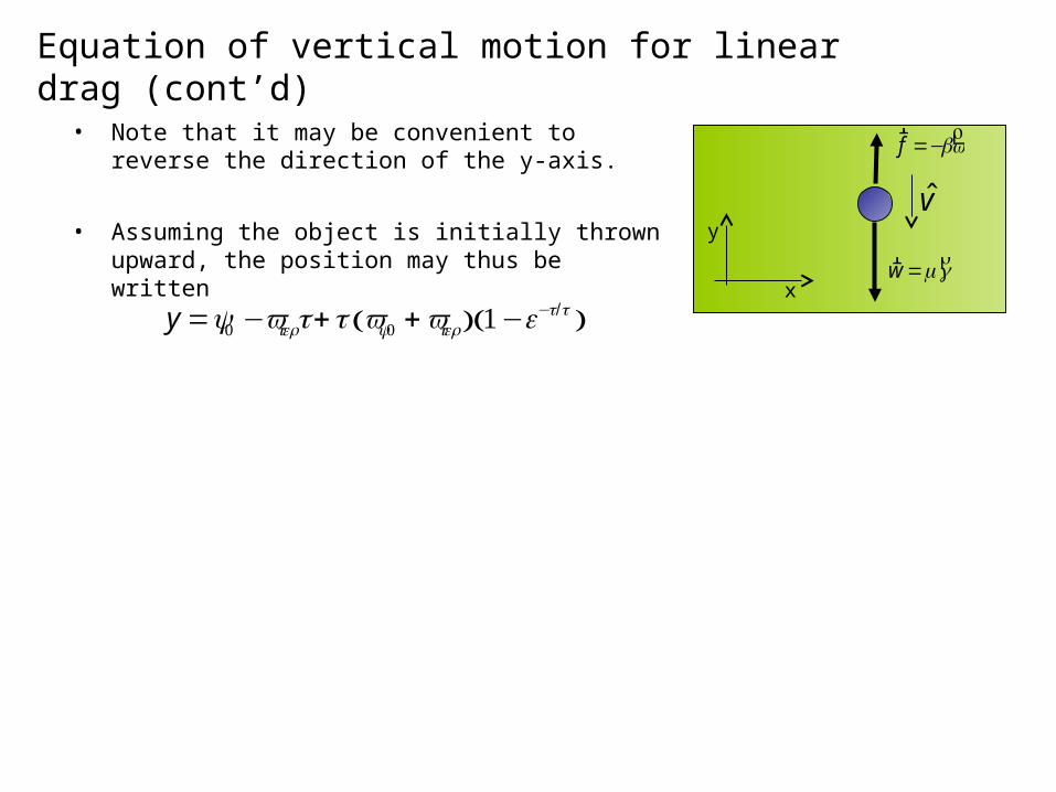
Equation of vertical motion for linear drag (cont’d)

• Note that it may be convenient to reverse the direction of the y-axis.

• Assuming the object is initially thrown upward, the position may thus be written

rw =m

rg

rf =−b

rv

v̂y

x

y =y0 −vtert+τ vy0 + vter( ) 1−e−t/τ( )

Equation of motion for linear drag (cont’d)

• Combine horizontal and vertical equations to get the trajectory of a projectile.

• To obtain an equation of the form y=y(x), solve the 1st equation for t, and substitute in the second equation.

x(t)=vx0τ 1−e−t/τ( )y(t)=y0 −vtert+τ vy0 + vter( ) 1−e−t/τ( )

y(t)=y0 +vy0 + vter

vx0

x+ vterτ ln 1−x

vx0τ⎛

⎝⎜⎞

⎠⎟

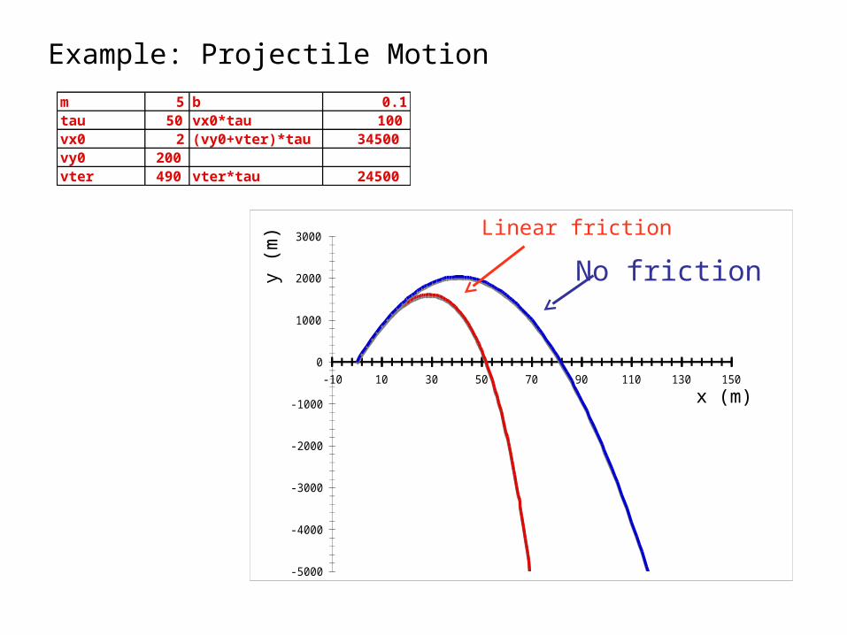
Example: Projectile Motion

m 5 b 0.1tau 50 vx0*tau 100vx0 2 (vy0+vter)*tau 34500vy0 200vter 490 vter*tau 24500

-5000

-4000

-3000

-2000

-1000

0

1000

2000

3000

-10 10 30 50 70 90 110 130 150

x (m)

y (m

)No friction

Linear friction

Horizontal Range

• In the absence of friction (vacuum), one has

• The range in vacuum is therefore

• For a system with linear drag, one has

x(t)=vxot

y(t) =vyot−0.982 t2

Rvac =2vxovyo

g

0 =vy0 + vter

vx0

R+ vterτ ln 1−R

vx0τ⎛

⎝⎜⎞

⎠⎟

A transcendental equation - cannot be solved analytically

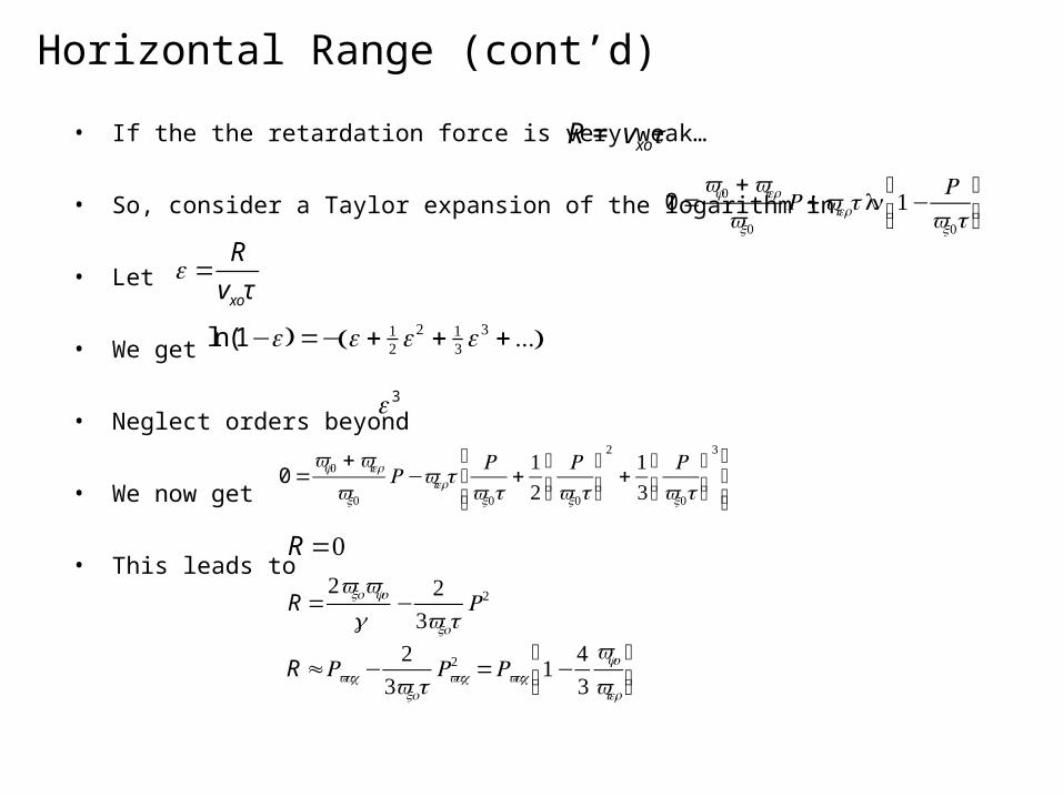
Horizontal Range (cont’d)

• If the the retardation force is very weak…

• So, consider a Taylor expansion of the logarithm in

• Let

• We get

• Neglect orders beyond

• We now get

• This leads to

R = vxoτ

0 =vy0 + vter

vx0

R+ vterτ ln 1−R

vx0τ⎛

⎝⎜⎞

⎠⎟

ε =R

vxoτ

ln(1−ε) =− ε + 12 ε

2 + 13 ε

3 + ...( )

ε 3

0 =vy0 + vter

vx0

R−vterτR

vx0τ+12

Rvx0τ

⎛

⎝⎜⎞

⎠⎟

2

+13

Rvx0τ

⎛

⎝⎜⎞

⎠⎟

3⎡

⎣⎢⎢

⎤

⎦⎥⎥

R =0

R =2vxovyo

g−

23vxoτ

R2

R ≈Rvac −2

3vxoτRvac

2 =Rvac 1−43

vyo

vter

⎛

⎝⎜⎞

⎠⎟

Quadratic Air Resistance

• For macroscopic projectiles, it is usually a better approximation to consider the drag force is quadratic

• Newton’s Law is thus

• Although this is a first order equation, it is NOT separable in x,y,z components of the velocity.

rf =−cv2rv

mr&v =m

rg−cv2rv

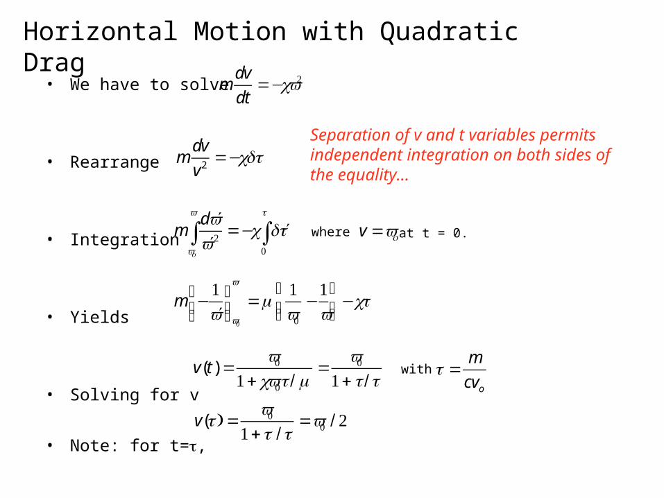
Horizontal Motion with Quadratic Drag

• We have to solve

• Rearrange

• Integration

• Yields

• Solving for v

• Note: for t=τ,

mdv

dt=−cv2

mdv

v2=−cdt

Separation of v and t variables permits independent integration on both sides of the equality…

md ′v′v 2

vo

v

∫ =−c d ′t0

t

∫ where v =vo at t = 0.

m −1′v

⎡⎣⎢

⎤⎦⎥v0

v

=m1v0

−1v

⎛

⎝⎜⎞

⎠⎟−ct

v(t)=v0

1+ cv0t / m=

v01+ t / τ

with τ =m

cvo

v(τ ) =v0

1+τ / τ=v0 / 2

Horizontal Motion with Quadratic Drag (cont’d)

• Horizontal position vs time obtained by integration …

• Never stops increasing

• By contrast to the “linear” case.

• Which saturates…

• Why? ! ?

• The retardation force becomes quite weak as soon as v<1.

• In realistic treatment, one must include both the linear and quadratic terms.

x(t)=x+ v( ′t )d ′t0

t

∫=v0τ ln(1+ t / τ )

0

2

4

6

8

10

12

0 5 10 15 20 25 30 35 40 45 50

0

10

20

30

40

50

60

70

0 5 10 15 20 25 30 35 40 45 50

v(t)=v0

1+ t / τ

x(t)=v0τ ln(1+ t / τ )

x(t)=vx0τ 1−e−t/τ( )

• Measuring the vertical position, y, down.

• Terminal velocity achieved for

• For the baseball of our earlier example, this yields ~ 35 m/s or 80 miles/hour

• Rewrite in terms of the terminal velocity

• Solve by separation of variables

• Integration yields

• Solve for v

• Integrate to find

Vertical Motion with Quadratic Drag

mdv

dt=mg−cv2

vter =mgc

dv

dt=g 1−

v2

vter2

⎛

⎝⎜⎞

⎠⎟

dv

1−v2

vter2

=gdt

vtergarctanh

v

vter

⎛

⎝⎜⎞

⎠⎟=t

v =vtertanhgtvter

⎛

⎝⎜⎞

⎠⎟

y =vter( )

2

gln cosh

gtvter

⎛

⎝⎜⎞

⎠⎟⎡

⎣⎢

⎤

⎦⎥

0

5

10

15

20

25

30

35

40

0 5 10 15 20 25 30

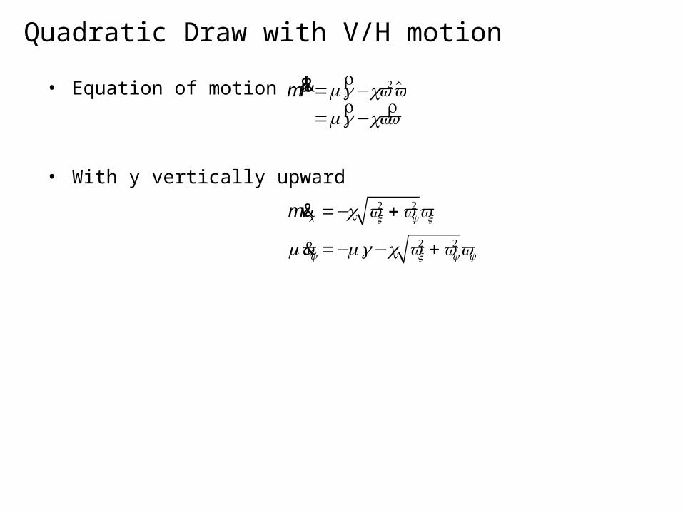
Quadratic Draw with V/H motion

• Equation of motion

• With y vertically upward

mr&&r =m

rg−cv2v̂

=mrg−cv

rv

m&vx =−c vx2 + vy

2vx

m&vy =−mg−c vx2 + vy

2vy

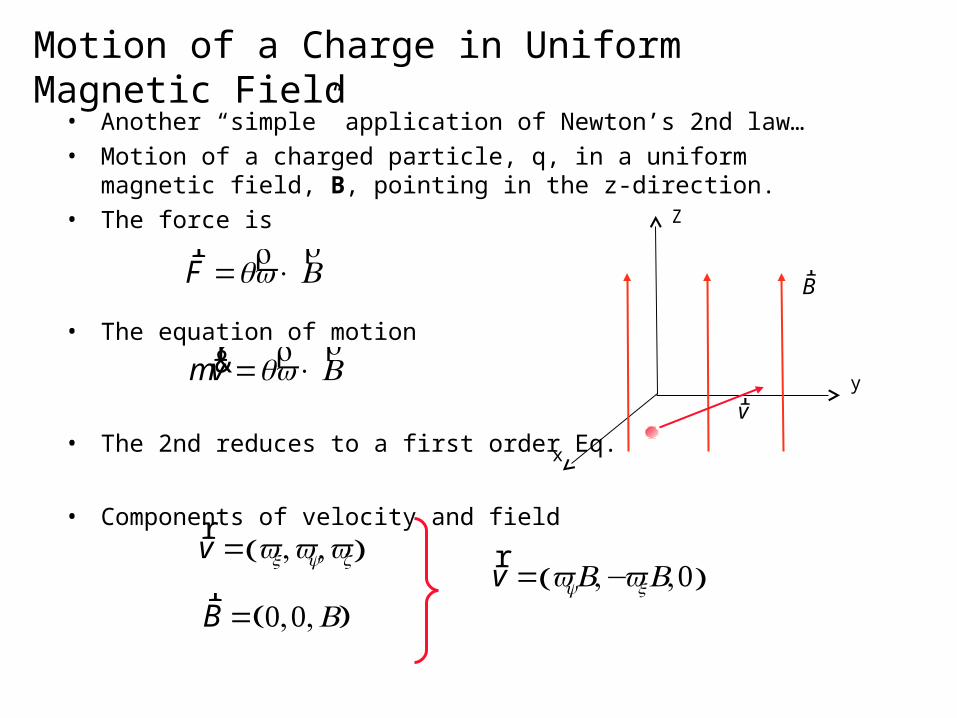
Motion of a Charge in Uniform Magnetic Field

• Another “simple” application of Newton’s 2nd law…

• Motion of a charged particle, q, in a uniform magnetic field, B, pointing in the z-direction.

• The force is

• The equation of motion

• The 2nd reduces to a first order Eq.

• Components of velocity and field

rF =q

rv×

rB

Z

x

y

rB

rv

mr&v =q

rv×

rB

rv = vx,vy,vz( )

rB = 0,0,B( )

rv = vyB,−vxB,0( )

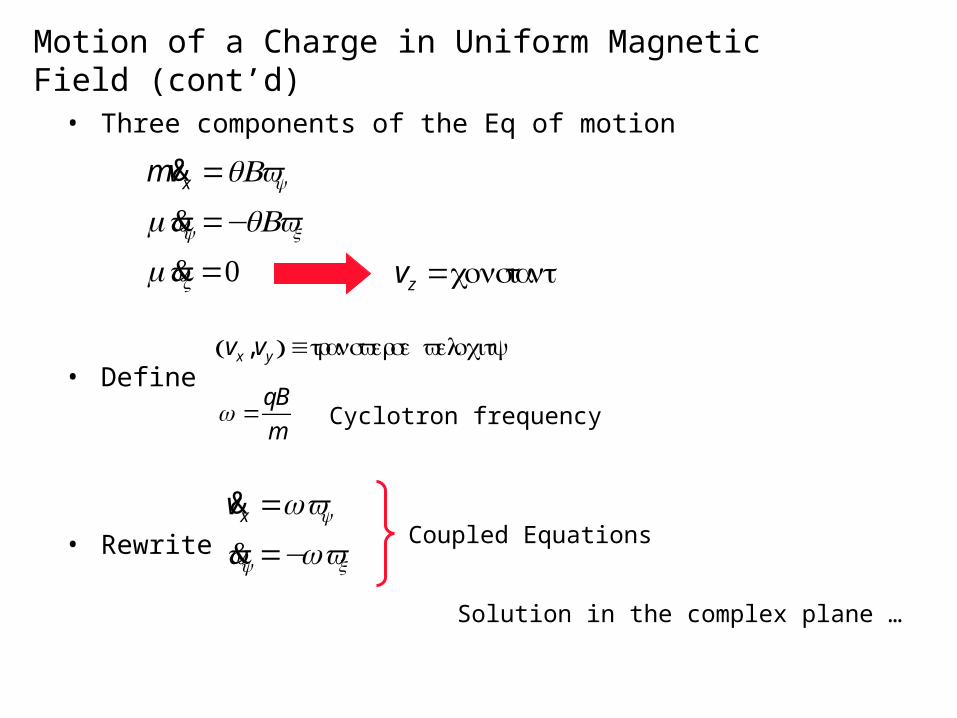
Motion of a Charge in Uniform Magnetic Field (cont’d)

• Three components of the Eq of motion

• Define

• Rewrite

m&vx =qBvy

m&vy =−qBvx

m&vz =0 vz =constant

ω =qB

m

vx ,vy( ) ≡transverse velocity

Cyclotron frequency

&vx =ωvy

&vy =−ωvx

Coupled Equations

Solution in the complex plane …

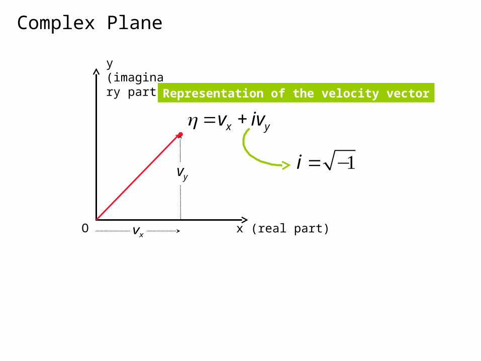
Complex Plane

O x (real part)

y (imaginary part)

=vx + ivy

vy

vx

Representation of the velocity vector

i = −1

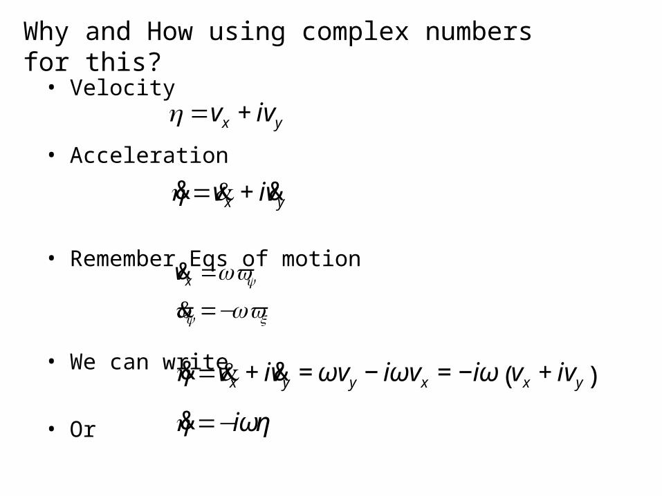
Why and How using complex numbers for this?

• Velocity

• Acceleration

• Remember Eqs of motion

• We can write

• Or

=vx + ivy

&vx =ωvy

&vy =−ωvx

& =&vx + i&vy

& =&vx + i&vy =ωvy − iωvx = −iω vx + ivy( )

& =−iωη

Why and How using … (cont’d)

• Equation of motion

• Solution

• Verify by substitution

& =−iωη

=Ae−iωt

ddt

=−iωAe−iωt =−iω

Complex Exponentials

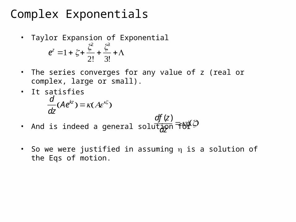
• Taylor Expansion of Exponential

• The series converges for any value of z (real or complex, large or small).

• It satisfies

• And is indeed a general solution for

• So we were justified in assuming is a solution of the Eqs of motion.

ez =1+ z+

z2

2!+

z3

3!+L

d

dzAekz( ) =k Aekz( )

df (z)

dz=kf(z)

Complex Exponentials (cont’d)

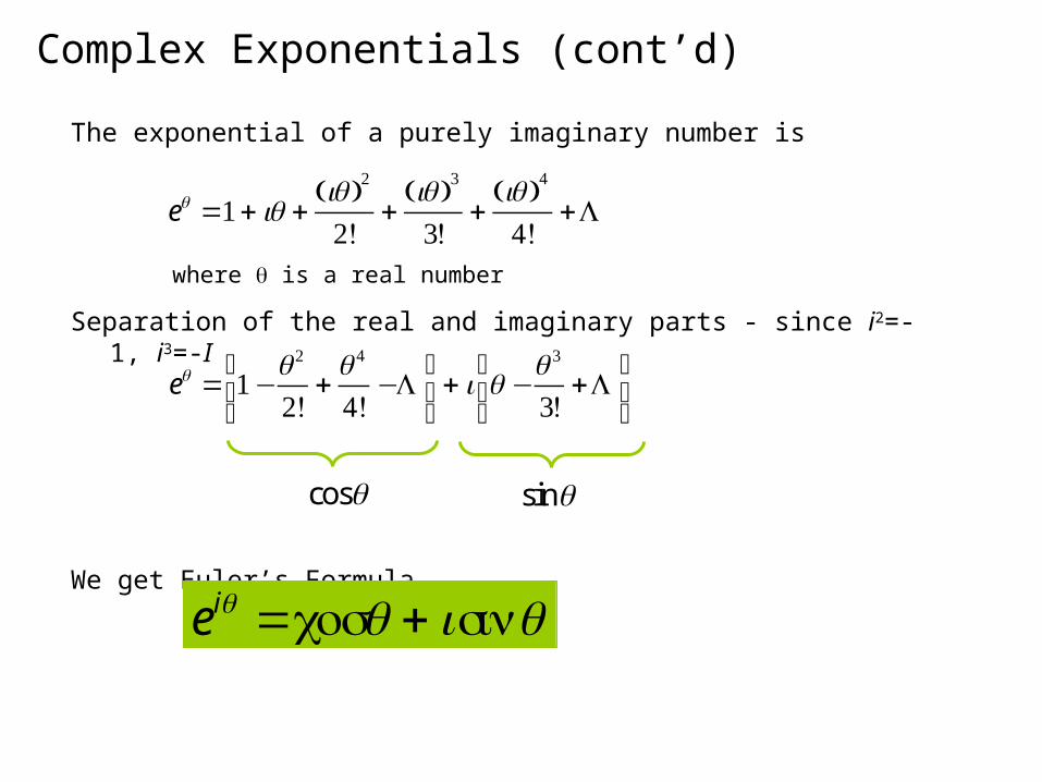
The exponential of a purely imaginary number is

Separation of the real and imaginary parts - since i2=-1, i3=-I

We get Euler’s Formula

eθ =1+ iθ +

iθ( )2

2!+

iθ( )3

3!+

iθ( )4

4!+L

where θ is a real number

eθ = 1−

θ 2

2!+θ 4

4!−L

⎡

⎣⎢

⎤

⎦⎥+ i θ −

θ 3

3!+L

⎡

⎣⎢

⎤

⎦⎥

cosθ sinθ

eiθ =cosθ + isinθ

Complex Exponentials (cont’d)

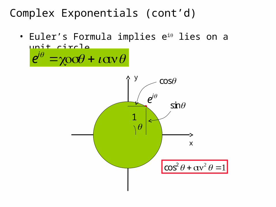
• Euler’s Formula implies eiθ lies on a unit circle.

O

x

y

eiθcosθ

sinθ1θ

eiθ =cosθ + isinθ

cos2θ + sin2θ =1

Complex Exponentials (cont’d)

• A complex number expressed in the polar form

O

x

y

A =aeiθ

acosθ

asinθa θ

A =aeiθ =acosθ + iasinθ

a2 cos2θ + a2 sin2θ =a2

where a and θ are real numbers

−iωt =Ae−iωt

=Ae−iωt = aei θ −ωt( )

Amplitude

Phase

Angular Frequency

Solution for a charge in uniform B field

• vz constant implies

• The motion in the x-y plane best represented by introduction of complex number.

• The derivative of

• Integration of

z(t)=zo + vzot

=x + iyGreek letter “xi”

& =&x + i&y = vx + ivy = η

= dt∫ = Ae−iωtdt∫

=iA

ωe−iωt + constant

x + iy=Ce−iωt + X+iY( )

Solution for a charge in uniform B field (cont’d)

x + iy=Ce−iωt + X+iY( )

Redefine the z-axis so it passes through (X,Y)

x + iy=Ce−iωt

which for t = 0, impliesC =xo + iyo

ω =qB

m

Motion frequency

O

x

y

xo + iyo

ωtx + iy

xo2 + yo

2

Solution for a charge in uniform B field (cont’d)

x(t)+ iy(t) =Ce−iωt

z(t)=zo + vzot

ω =qB

m

O

x

y

xo + iyo

ωt

x + iy

xo2 + yo

2

Helix Motion