Newtonian Mechanics - Physics & Astronomyhomepage.physics.uiowa.edu/~wpolyzou/phys205/205_… ·...

Chapter 1

Newtonian Mechanics

1.1 Definitions

Classical Mechanics is the theory governing the motion of particles. The theoryis unchanged since it’s discovery by Newton.

Point particles are idealized particles whose internal dimensions and prop-erties can be neglected. The motion of a point particle can be completelydescribed by the particle’s position as a function of time in some coordinatesystem. The coordinates of the particle’s position is denoted by a vector x(t).

The particle’s instantaneous velocity v(t) and acceleration a(t) in this coor-dinate system are defined by

v(t) =dx

dt(t) (1.1)

a(t) =d2x

dt2(t). (1.2)

I use MKS units where distance is measured in meters, mass is measured inkilograms and time is measured in seconds.

1.2 Experimental observations

1.2.1 Principle of Newtonian determinacy and Newton’ssecond law

A fundamental observation (recognized by Newton and nicely discussed in Arnold’sbook) is that the particle’s position, x(t), is a function that depends only onthe time t and the coordinate and velocity of the particle at some earlier initial,time t = t0. Arnold refers to this observation as the principle of Newtoniandeterminacy. This can be written mathematically as

x(t) = X(t, t0,x(t0),v(t0)). (1.3)

1

2 CHAPTER 1. NEWTONIAN MECHANICS

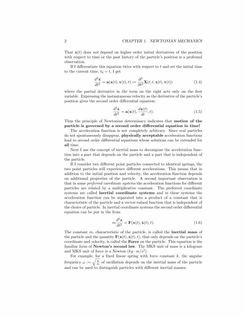
That x(t) does not depend on higher order initial derivatives of the positionwith respect to time or the past history of the particle’s position is a profoundobservation.

If I differentiate this equation twice with respect to t and set the initial timeto the current time, t0 = t, I get

d2x

dt2= a(x(t),v(t), t) :=

∂2

∂t2X(t, t,x(t),v(t)) (1.4)

where the partial derivative in the term on the right acts only on the firstvariable. Expressing the instantaneous velocity as the derivative of the particle’sposition gives the second order differential equation:

d2x

dt2= a(x(t),

dx(t)

dt, t). (1.5)

Thus the principle of Newtonian determinacy indicates that motion of theparticle is governed by a second order differential equation in time!

The acceleration function is not completely arbitrary. Since real particlesdo not spontaneously disappear, physically acceptable acceleration functionslead to second order differential equations whose solutions can be extended forall time.

Next I use the concept of inertial mass to decompose the acceleration func-tion into a part that depends on the particle and a part that is independent ofthe particle.

If I consider two different point particles connected to identical springs, thetwo point particles will experience different accelerations. This means that inaddition to the initial position and velocity, the acceleration function dependson additional properties of the particle. A second important observation isthat in some preferred coordinate systems the acceleration functions for differentparticles are related by a multiplicative constant. The preferred coordinatesystems are called inertial coordinate systems and in these systems theacceleration function can be separated into a product of a constant that ischaracteristic of the particle and a vector-valued function that is independent ofthe choice of particle. In inertial coordinate systems the second order differentialequation can be put in the from

md2x

dt2= F(x(t), x(t), t). (1.6)

The constant m, characteristic of the particle, is called the inertial mass ofthe particle and the quantity F(x(t), x(t), t), that only depends on the particle’scoordinate and velocity, is called the Force on the particle. This equation is thefamiliar form of Newton’s second law. The MKS unit of mass is a kilogramand MKS unit of force is a Newton (kg ·m/s2).

For example, for a fixed linear spring with force constant k, the angular

frequency ω :=√

km of oscillation depends on the inertial mass of the particle

and can be used to distinguish particles with different inertial masses.

1.2. EXPERIMENTAL OBSERVATIONS 3

The inertial mass permits a clean separation of the acceleration function intoa part the depends of properties of the particle and a part that depends of theinitial conditions and the rest of the system on the right.

These considerations generalize to systems of N interacting point particles.The resulting second order differential equation has the form

mid2xi

d2x= Fi(x1 · · ·xN ;

dx

dt 1· · · dx

dt N, t) (1.7)

In this case the particle’s coordinate as a function of time, xi(t), is the solution of3N coupled second-order differential equations. The solution requires specifyingthe initial coordinates and velocities of all N particles.

1.2.2 Local solutions

The equations of motion (1.6) can be equivalently expressed as a system of 6Ncoupled first order differential equations

dvi

dt=

1

miFi(x1, · · ·xN ,v1, · · · ,vN , t) (1.8)

dxi

dt= vi. (1.9)

Integrating these equations from t0 to t gives an equivalent system of integralequations that incorporate the initial coordinate and velocity:

vi(t) = vi(t0) +

∫ t

t0

1

miFi(x1(t

′), · · ·xN (t′),v1(t′), · · · ,vN (t′), t′)dt′ (1.10)

xi(t) = xi(t0) +

∫ t

t0

vi(t′)dt′. (1.11)

For small t− t0 this system can be solved by iteration. The iterative solution isgiven by

vi(t) = limk→∞

vki (t) (1.12)

xi(t) = limk→∞

xki (t) (1.13)

where the initial values arev0i (t) = vi(t0) (1.14)

x0i (t) = xi(t0) (1.15)

and the k-th approximations can be expressed in terms of the k − 1-th approx-imation as

vki (t) = vi(t0) +

∫ t

t0

1

miFi(x

k−11 (t′), · · ·xk−1

N (t′),vk−11 (t′), · · · ,vk−1

N (t′), t′)dt′

(1.16)


xki (t) = xi(t0) +

∫ t

t0

vk1i (t′)dt′. (1.17)

This is just the iteration used by Picard to prove the existence of local solutionsof systems of differential equations. The convergence of this method has onlybeen established for sufficiently small t − t0. It is much more difficult to findstable computational methods for finding solutions that are valid for all time,however independent of mathematical considerations, physics considerations re-quire that acceptable physical forces must be of the type that have solutionsthat are valid for all time.

1.2.3 Galilean invariance

A third important observation is called the Principle of Galilean Relativity.It states that for isolated systems the form of the dynamical equations is thesame in all inertial coordinate systems.

For the special case of a single point particle in the absence of forces theequation of motion in an inertial coordinate system is

d2x

dt2= 0. (1.18)

The form of this equation must be the same in any inertial coordinate system.The form of equation (1.18) is preserved by (1) changing the origin of the

coordinate system by a fixed constant vector (2) changing the origin of thecoordinate system by a fixed constant velocity (3) rotating the coordinate systemabout a fixed point (4) or changing the time by a fixed amount. Combining thesetransformations defines a new inertial coordinate system:

xi → x′i = Rxi + vt+ x0 (1.19)

t → t′ = t+ c. (1.20)

Transformations generated by these elementary transformations are calledGalileantransformations. Here R is a 3× 3 orthogonal matrix with unit determinant.The orthogonality ensures that it preserves the length of vectors and the con-dition on the determinant ensures that it does not include transformations thatinvolve space reflection. Later I will show that these transformations are rota-tions.

It is an easy exercise to show (1) the composition of two Galilean transforma-tions is Galilean (2) the identity is a Galilean transformation (3) every Galileantransformation has an inverse (4) the composition of Galilean transformationsis associative.

These properties imply that the Galilean transformations define a mathe-matical structure called a group under composition. This is called the Galileangroup. The elements of this group are coordinate transformations relate differ-ent inertial coordinate systems.


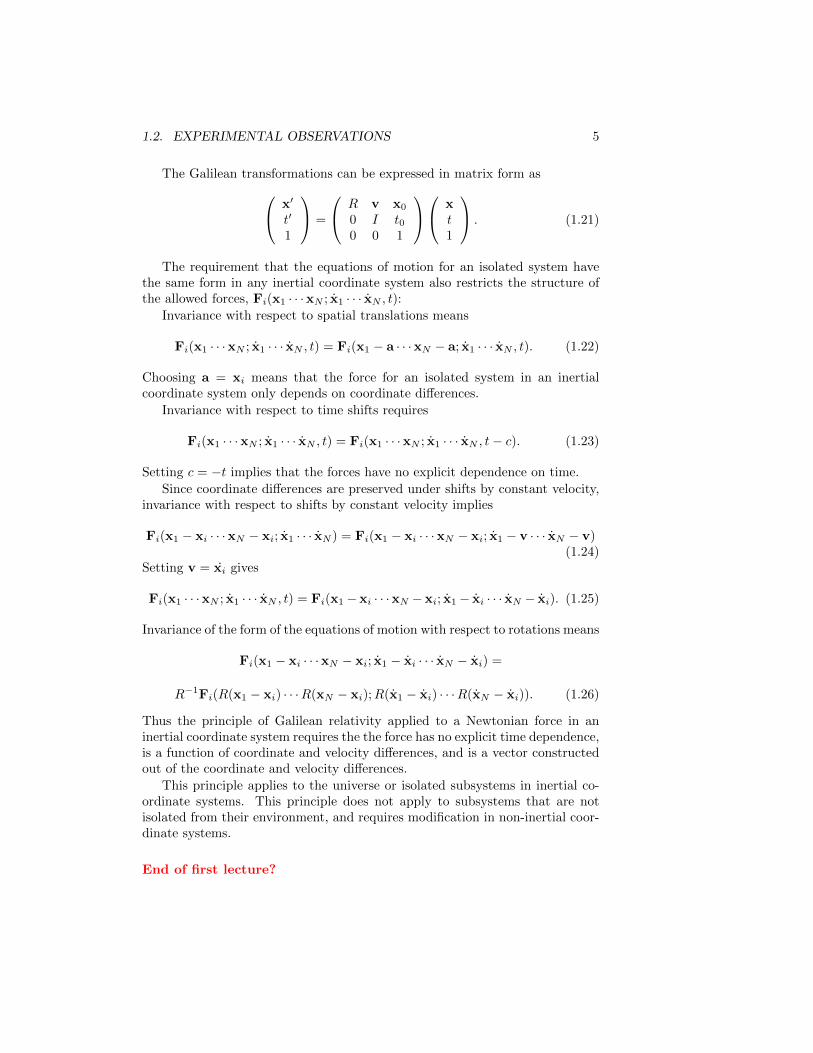
The Galilean transformations can be expressed in matrix form as x′

t′

1

=

R v x0

0 I t00 0 1

xt1

. (1.21)

The requirement that the equations of motion for an isolated system havethe same form in any inertial coordinate system also restricts the structure ofthe allowed forces, Fi(x1 · · ·xN ; x1 · · · xN , t):

Invariance with respect to spatial translations means

Fi(x1 · · ·xN ; x1 · · · xN , t) = Fi(x1 − a · · ·xN − a; x1 · · · xN , t). (1.22)

Choosing a = xi means that the force for an isolated system in an inertialcoordinate system only depends on coordinate differences.

Invariance with respect to time shifts requires

Fi(x1 · · ·xN ; x1 · · · xN , t) = Fi(x1 · · ·xN ; x1 · · · xN , t− c). (1.23)

Setting c = −t implies that the forces have no explicit dependence on time.

Since coordinate differences are preserved under shifts by constant velocity,invariance with respect to shifts by constant velocity implies

Fi(x1 − xi · · ·xN − xi; x1 · · · xN ) = Fi(x1 − xi · · ·xN − xi; x1 − v · · · xN − v)(1.24)

Setting v = xi gives

Fi(x1 · · ·xN ; x1 · · · xN , t) = Fi(x1 −xi · · ·xN −xi; x1 − xi · · · xN − xi). (1.25)

Invariance of the form of the equations of motion with respect to rotations means

Fi(x1 − xi · · ·xN − xi; x1 − xi · · · xN − xi) =

R−1Fi(R(x1 − xi) · · ·R(xN − xi);R(x1 − xi) · · ·R(xN − xi)). (1.26)

Thus the principle of Galilean relativity applied to a Newtonian force in aninertial coordinate system requires the the force has no explicit time dependence,is a function of coordinate and velocity differences, and is a vector constructedout of the coordinate and velocity differences.

This principle applies to the universe or isolated subsystems in inertial co-ordinate systems. This principle does not apply to subsystems that are notisolated from their environment, and requires modification in non-inertial coor-dinate systems.

End of first lecture?


1.2.4 Inertial reference frames

The group of Galilean transformations tells one how to transform from oneinertial frame to another one, but it does not give any indication of how toexperimentally determine if a given frame is inertial. To answer this question itis useful to consider how the equations of motion are modified in a non-inertialcoordinate system.

1.2.5 Accelerated reference frames

To understand this problem it is useful to postulate a dynamics formulatedin a fixed inertial reference frame and consider how the dynamics looks in anarbitrary frame.

I consider general coordinates yi related to inertial coordinates xi by

yi = yi(xi, t). (1.27)

To use Newton’s laws in an inertial coordinate system I compute the first andsecond time derivatives of these coordinates:

dyi

dt=∑j

∂yi

∂xji

dxji

dt+

∂yi

∂t(1.28)

d2yi

dt2=∑j

∂yi

∂xji

d2xji

dt2+∑jk

∂2yi

∂xji∂x

ki

dxji

dt

dxki

dt+

2∑j

∂2yi

∂xji∂t

dxji

dt+

∂2yi

∂t2. (1.29)

Multiplying by mi and using Newton’s second laws in an inertial coordinatesystem gives

mid2yi

dt2=∑j

∂yi

∂xji

F ji +mi

∑kj

∂2yi

∂xji∂x

ki

dxji

dt

dxki

dt+

2mi∂2yi

∂xji∂t

dxji

dt+mi

∂2yi

∂t2. (1.30)

This equation looks like Newton’s second law with a transformed force∑j

∂yi

∂xji

F ji (1.31)

and three additional inertial forces:

F1 := mi

∑kj

∂2yi

∂xji∂x

ki

dxji

dt

dxki

dt(1.32)


F2 :=∑j

2mi∂2yi

∂xji∂t

dxji

dt(1.33)

and

F3 := mi∂2yi

∂t2. (1.34)

The inertial forces can be distinguished from the transformed force by the ap-pearance of the inertial mass mi in these forces. In addition they do not vanishwhen Fi = 0. This means that particles in non-inertial coordinate systems willexperience spontaneous acceleration in the absence of applied forces.

These inertial forces are familiar. They include the force that pushes youback in you seat when an airplane takes off.

This equation suggest that a coordinate system for an isolated system isinertial if in that coordinate system a particle’s acceleration is inversely pro-portional to its inertial mass. Clearly, for the inertial forces the acceleration isindependent of the mass, so non-inertial frames do not have this property.

1.2.6 Gravity

The problem with the test described above is that while it works fine for elec-trical forces, it fails for gravitational forces. This is because of the remarkableobservation that the gravitational “charge” of a particle is identical to its inertialmass. As a consequence of the equivalence of the inertial and gravitationalmass the masses cancel on both sides of the equation and the particle’s accel-eration is independent of its mass in all coordinate systems. The equivalence ofthe gravitational and inertial mass is not explained by classical mechanics. Inclassical mechanics both masses have very difference origins. This observationis a consequence of the theory of general relativity.

1.2.7 Newton’s first law

If the force on a particle in an inertial coordinate system vanishes, then theparticle’s acceleration is zero. Integrating this differential equation (1.6) withno force term gives

x(t) = v(t0)(t− t0) + x(t0) (1.35)

which means that the particle moves with constant velocity. This is the contentof Newton’s first law.

1.2.8 Conservative forces

Many forces in nature are independent of velocities and are derivable from asingle-valued potential function. I consider potential functions that do not de-pend on the particle velocities. A set of forces are conservative if they can bewritten in the form

Fi = − ∂

∂xiV (x1 · · ·xN ) (1.36)


for some single valued potential function V (x1 · · ·xN ).

The work done, WA,B [γγγ], by a force along some path γγγ(λ) between xA andxB is

WA,B [γγγ] :=

∫γγγ

F · dx =

∫ 1

0

F · dγγγ

dλdλ (1.37)

where γγγ(0) = xA and γγγ(1) = xB .

For a system of particles this is replaced by

WA,B [γγγ] :=∑i

∫γγγi

Fi · dxi =

∫ 1

0

∑i

Fi ·dγγγi

dλdλ. (1.38)

where γγγi(0) = xiA and γγγi(1) = xiB .

The work done by a conservative force is independent of the paths used toget from the initial to the final points.

WA,B [γγγ] :=

∫ 1

0

∑i

Fi ·dγγγi

dλdλ =

∫(−∇∇∇iV (γγγ1(λ)γγγN (λ)) · dγ

γγi

dλdλ = (1.39)

∫ 1

0

d

dλV (γγγ1(λ) · · ·γγγN (λ))dλ =

V (γγγ1(1) · · ·γγγN (1))− V (γγγ1(0) · · ·γγγN (0)) =

V (x1A, · · · ,xNA)− V (V (x1B , · · · ,xNB)) (1.40)

which only depends on the endpoints of the paths, not the specific path.

For a closed path, xiA = xiA

γγγ1(1) = γγγ1(0) (1.41)

and for a single-valued potential

V (γγγ1(1) · · ·γγγN (1))− V (γγγ1(0) · · ·γγγN (0)) =

V (x1A, · · · ,xNA)− (V (x1A, · · · ,xNA)) = 0 (1.42)

This can be expressed in the form

∑i

∮γγγi

Fi · dxi = 0 (1.43)

for any closed path γ = (γγγ1(λ), . . . , γγγN (λ)).


1.2.9 Newton’s third law

For a Galilean invariant systems interacting with velocity-independent conser-vative forces the potential only depends on the coordinate differences. Thismeans that the potential functions satisfy

V (x1, · · · ,xN , t) = V (x1 − xN , · · · ,xN−1 − xN , t). (1.44)

It follows that the net force on this system is

N∑i=1

Fi =

N−1∑i=1

(∂V

∂xi− ∂V

∂xi) = 0. (1.45)

Which shows that the net force on a translationally invariant conservative sys-tem with velocity independent forces is zero. When applied to isolated systemsof two particles it means that the force on particle 1 due to particle 2 is thenegative of the force on particle 2 due to article 1. This is the usual form ofNewton’s third law.

1.2.10 Macroscopic particles - elementary conservation laws

Consider a macroscopic particle consisting of many point particles. Assume thateach point particle experiences (1) an applied external force and (2) Galileaninvariant conservative forces due the other point particles in the system.

I define the total inertial mass

M :=∑i

mi (1.46)

and the center of mass coordinate

X :=∑i

mi

Mxi (1.47)

In terms of these quantities

Md2X

dt2=∑i

Mmi

M

d2xi

dt2=∑i

mid2xi

dt2=∑i

Fi (1.48)

Fi = − ∂V

∂xi+ Fi ext (1.49)

The sum of the derivatives of the potential vanishes (1.45) due to the Galileaninvariance of the conservative inter-particle forces. It follows that the total forceon the macroscopic particle is the vector sum of the applied external forces onthe system. Summing over the particles gives∑

i

Fi = −∑i

∂V

∂xi+∑i

Fi ext (1.50)


It follows that

Md2X

dt2=∑i

Fi ext (1.51)

which as the form of Newton’s second law for a point particle of mass M andcoordinate X being acted on by a force Fext :=

∑i Fi ext.

The means the center of mass coordinate of the system behaves like a pointparticle being acted on by the sum of the external forces on the system. Thisjustifies treating a macroscopic system of point particles by an idealized pointparticle. This is independent of all of relative motion of the constituent pointparticles.

1.2.11 Conservation Laws

Symmetries in classical mechanics are normally associated with conserved quan-tities.

In the above analysis the translational invariance of conservative force en-sures that the corresponding potential was only a function of coordinate dif-ferences. This in turn showed that the sum of all of the inter-particle forcesvanish.

In the absence of external forces equation (??) becomes

Md2X

dt2=

d

dt

(M

dX

dt

)= 000 (1.52)

The conserved vector quantity

P = MdX

dt(1.53)

is called the linear momentum of the system. The above equation showsthat all three components are conserved in the absence of external forces.

From the definitions it follows that

P = MdX

dt=∑i

midxi

dt:=∑i

pi (1.54)

where pi := midxi

dt is the linear momentum of particle i.The quantity

L := X×P (1.55)

is called the angular momentum of the system. Note that its value dependson the position of the origin of the coordinate system. Note that for an isolatedGalilean-invariant system

dL

dt:=

dX

dt×P+X× dP

dt=

1

MP×P+X× Fext = X× Fext. (1.56)

this vanishes in the absence of external forces or more generally when the ex-ternal torque

T := X× Fext (1.57)


vanishes. It follows that in the absence of external torques the angular momen-tum of the system

L := X×P (1.58)

is conserved. The last conservation law follows from

000 = Md2X

dt2· dXdt

=1

2M

d

dt(dX

dt· dXdt

) =1

2MP ·P (1.59)

which shows that in the absence of external forces the total kinetic energy isconserved.

These conservation laws hold for isolated systems or isolated point particles.We will discuss a more general treatment of conservation laws in the next section.

End second lecture

Chapter 2

Lagrangian Dynamics

2.1 Problems with constraints

Many mechanical system involve constraints. In addition to explicit forces, thesystem also has forces due to the constraints that are often not explicitly known.

There are many different kinds of constraints that may be relevant for anisolated system. A holonomic constraint is a relation of the form

f(x1, · · · ,xN , t) = 0 (2.1)

that constrains the particle’s coordinates. The time dependence means thatthese constraints can depend on time. Not all constraints are holonomic. Someelementary examples of non-holonomic constraints are

x2 + y2 ≤ L2

f(dx1

dt , · · · ,dxN

dt , t) = 0∑u ci(x1, · · · ,xN ) · dxi = 0 (unless ci =

∂g∂xi

for some g).

The method that I discuss for treating holonomic constraints can also be appliedto the third kind of constraint listed above, called differential constraints.

There are two problems when a system is subject to holonomic constraints.

1. Because of the constraints, not all of the coordinates are independent.

2. The forces of constraint are not explicitly known.

An important observation that helps to solve both of these problems is thatthe motion is normally perpendicular to the forces of constraint, so the con-straint forces do no work. For example, the normal force on an inclined planekeeps the particle on the plane, but it does no work as the particle slides downthe plane.

13

14 CHAPTER 2. LAGRANGIAN DYNAMICS

2.2 Principle of virtual work

I begin by considering a system of N point particles. Newton’s second lawimplies

dpi

dt− Fi = 0 (2.2)

Here Fi represents the sum of all of the forces on particle i including the con-straint forces. It follows that for an arbitrary infinitesimal displacement, δxi

that

(dpi

dt− Fi) · δxi = 0 (2.3)

Next I write the force on particle i as the sum of an applied force, Fai , and

a constraint force, Fci

(dpi

dt− Fa

i − Fci ) · δxi = 0. (2.4)

I also restrict the infinitesimal displacements so they are consistent with theconstraints. This requirement, along with the observation that the forces ofconstraint are perpendicular to the displacement, implies

Fci · δxi = 0. (2.5)

Thus, for infinitesimal displacements consistent with the constraints, equa-tion (2.4) becomes

(dpi

dt− Fa

i ) · δxi = 0. (2.6)

This step has eliminated the forces of constraint from the problem.If the system has K holonomic constraints then it is possible, by eliminating

variables, to express coordinates consistent with the constraints in terms of3N −K generalized coordinates, q1 · · · qm=3N−K :

xi = xi(q1, · · · , qm) (2.7)

Arbitrary small displacements consistent with the constraints can be ex-pressed as

δxi =∑j

∂xi

∂qjδqj (2.8)

where the small displacements in the 3N −K generalized coordinates are inde-pendent. Thus for each i

(dpi

dt− Fa

i ) ·∑j

∂xi

∂qjδqj = 0. (2.9)

If I sum (2.9) over i, because of the independence of the δqi, the coefficient ofeach δqi must vanish. This gives the following 3N −K = m equations:∑

i

(dpi

dt− Fa

i )∂xi

∂qj= 0 (2.10)

2.2. PRINCIPLE OF VIRTUAL WORK 15

for 1 ≤ j ≤ m.Now I use some elementary calculus to express (2.9) and (2.10) in a more

useful form: ∑i

dpi

dt· ∂xi

∂qk=∑i

d

dt(mi

dxi

dt) · ∂xi

∂qk=

∑i

d

dt(mi

dxi

dt· ∂xi

∂qk)−

∑i

midxi

dt· d

dt(∂xi

∂qk) (2.11)

Note thatd

dt(∂xi

∂qk) =

∂2xi

∂qk∂ql

dqldt

+∂2xi

∂qk∂t=

∂

∂qk(∂xi

∂ql

dqldt

+∂xi

∂t) =

∂

∂qk(dxi

dt) (2.12)

I also observe that because

dxi

dt=

∂xi

∂ql

dqldt

+∂xi

∂t(2.13)

it follows that∂xi

∂ql=

∂xi

∂ql, (2.14)

where ql =dqldt and xi =

dxi

dt .Using (2.11-2.14) in (2.10) gives

0 =∑i

(dpi

dt− Fa

i ) ·∑j

∂xi

∂qj=

∑i

mi

(d

dt(dxi

dt· ∂xi

∂qj)− dxi

dt· d

dt(∂xi

∂qj)

)−∑i

Fai ·∑j

∂xi

∂qj=

∑i

mi

(d

dt(dxi

dt· ∂xi

∂qj)− dxi

dt· ( ∂

∂qj(dxi

dt)

)−∑i

Fai ·∑j

∂xi

∂qj=

d

dt

∂

∂qj(∑i

1

2mi

dxi

dt· dxi

dt)− ∂

∂qj(∑i

1

2mi

dxi

dt· dxi

dt)−

∑i

Fai ·∑j

∂xi

∂qj=

(d

dt

∂

∂qj− ∂

∂qj

)T −

∑i

Fai ·∑j

∂xi

∂qj(2.15)

where T is the kinetic energy of the system:

T :=∑i

1

2mi

dxi

dt· dxi

dt(2.16)

With these substitutions equation (2.9) becomes∑j

((d

dt

∂

∂qj− ∂

∂qj)T −Qj

)δqj = 0 (2.17)


and equation (2.10) becomes(d

dt

∂

∂qj− ∂

∂qj

)T = Qj (2.18)

where

Qj :=∑i

Fai ·

∂xi

∂qj(2.19)

is called called a generalized force. When the applied force is conservativethen the generalized force takes on a simple form

Qj :=∑i

Fai ·

∂xi

∂qj=

−∑i

∂V

∂xi· ∂xi

∂qj= −∂V

∂qj(2.20)

Since the potential is independent of velocities I can replace (2.20) by

Qj =

(d

dt

∂

∂qj− ∂

∂qj

)V (2.21)

Using this in (??) gives the following system of equations(d

dt

∂

∂qj− ∂

∂qj

)(T − V ) = 0 (2.22)

The quantity L = T − V is called the Lagrangian of this system. The differ-ential equations (2.22) are called Lagrange’s equations. The standard formof Lagrange’s equations is

d

dt

∂L

∂qj− ∂L

∂qj= 0. (2.23)

For a conservative force equation (2.9) becomes∑j

(d

dt

∂L

∂qj− ∂L

∂qj)δqj = 0. (2.24)

For conservative forces these equations are equivalent to Newton’s secondlaw. One advantage of Lagrange’s equations is that the dynamical input isa single scalar quantity L rather than a number of vector forces. A secondadvantage is that in the Lagrangian formulation it is not necessary to knowthe forces of constraint to find the equation of motion of the particle. Finally,the Lagrangian allows one to use any set of convenient generalized coordinates.This is true even when there are no constraints on the system.

End third lecture?

2.2. PRINCIPLE OF VIRTUAL WORK 17

2.2.1 Forces of constraint - Lagrange multipliers

Lagrange’s equations have the feature that the forces of constraint never appearin the equations of motion. Sometimes it is desirable to know the forces ofconstraint. For example, in designing a roller coaster it is important to knowthat the cart stays on the track. The signal for failure is the normal force, whichis a force of constraint, vanishes.

If I return to the principle of virtual work but replace the independent gener-alized coordinates by the full set of generalized coordinates, still assuming thatthe motion is consistent with the constraints, equation (2.9) is replaced by

3N∑j=1

(d

dt

∂L

∂qj− ∂L

∂qj

)δqj = 0. (2.25)

This differs from equation (2.9) in that the sum runs over all 3N generalizedcoordinates, however in this case we cannot demand that the coefficient of eachδqi vanish because they are no longer independent.

The holonomic constraints can be expressed in terms of the full set of gen-eralized coordinates as:

fi(q1 · · · q3N ) = 0 1 ≤ i ≤ k. (2.26)

Because there are k constraints we expect that there are only 3N−k independentgeneralized coordinates. The constraints imply the k additional relations

3N∑j=1

∂fi(q1 · · · q3N )

∂qjδqj = 0 (2.27)

for any displacements δqj consistent with the constraints.I add zero to equation (2.25) using some undetermined coefficients λi mul-

tiplied by (2.27) for each 1 ≤ i ≤ k I get

3N∑j=1

(d

dt

∂L

∂qj− ∂L

∂qj−

k∑i=1

λi∂fi(q1 · · · q3N )

∂qj

)δqj = 0. (2.28)

This is valid for any λi as long as the particles move in a manner that is consis-tent with the constraints. I choose the k λi’s so that for each time the coefficientof δqj for 3N − k + 1 ≤ j ≤ 3N is zero. It follows that

d

dt

∂L

∂qj− ∂L

∂qj−

k∑i=1

λi∂fi(q1 · · · q3N )

∂qj= 0 (2.29)

for j = 3N − k + 1 · · · 3N by the choice of λ. For this choice of the Lagrangemultipliers λi the last k terms in the sum in (2.28) do not appear. Theremaining 3N − k δqi in the sum can be taken as the independent generalized


coordinates It follows that the coefficients of each of them also vanish. Thisgives

d

dt

∂L

∂qj− ∂L

∂qj−

k∑i=1

λi∂fi(q1, · · · , q3N )

∂qj= 0 (2.30)

for j = 1 · · · 3N − k.While the interpretation of the first 3N − k and last k equations differ, the

result is the system of 3N equations:

d

dt

∂L

∂qj− ∂L

∂qj−

k∑i=1

λi∂fi(q1 · · · q3N )

∂qj= 0 (2.31)

for 1 ≤ j ≤ 3N . When the k constraints are used in these equations we getequations that we can solve for the Lagrange multipliers, λi. Comparing (2.31to (2.18) gives explicit expressions for the generalized forces of constraint:

d

dt

∂L

∂qj− ∂L

∂qj=

k∑i=1

λi∂fi(q1 · · · q3N )

∂qj= Qjconstraint 1 ≤ j ≤ 3N −k (2.32)

Note that unlike equation (2.24) equations (2.32) involve all 3N generalizedcoordinates with explicit constraint forces.

This method is called the method of Lagrange undetermined multipliers.Note that generalized forces can depend on both coordinates and velocities.

2.3 Dissipative forces

Many dissipative forces in nature are velocity dependent. In many cases ofinterest it is possible express all of the dissipative forces of a system in terms ofa single scalar function, P , of the coordinates and velocities

Fdi =

∂P

∂xi(2.33)

This is true, for example when the dissipative force on particle i depends onlythe velocity of particle i and coordinates of all of the particles. Even when thedissipative forces are not velocity-dependent they can be put in this form.

For this type of dissipative force

Qj :=∑i

Fai ·

∂xi

∂qj=∑i

∂P

∂xi· ∂xi

∂qj(2.34)

Using (2.14) this becomes

Qj =∑i

∂P

∂xi· ∂xi

∂qj=

∂P

∂qj. (2.35)

2.3. DISSIPATIVE FORCES 19

It follows that the equations of motion for combined conservative and dissipativeforces become (

d

dt

∂

∂qj− ∂

∂qj

)L =

∂P

∂qj(2.36)

An example of a useful class of dissipation functions P are

P = −∑i

αi

n(xi · xi)

n/2 (2.37)

where n = 1 gives static friction forces and n = 2 gives viscous forces.

2.3.1 Principle of stationary action

There is an alternate way to derive Lagrange’s equations. The derivation isbased on a variational principle that has applications that go beyond Newtonianmechanics.

A functional is a mapping from a space of functions with certain propertiesto the space of real or complex numbers. A simple example is

F [f ] = f(0) +

∫(f2(x) +

df

dx(x))dx. (2.38)

For mechanics applications we consider a system that can be described by spec-ifying the values of N generalized coordinates, {qi}Ni=1. Let γi(t) = qi be apath that gives the value of the i − th generalized coordinate of the system asa function of time subject to the initial and final conditions: γi(t0) = qAi andγi(tf ) = qBi .

The Action functional, A[γγγ], assigns a real number to a fixed collection ofpaths {γi(t)}. It is defined as

A[γγγ] :=

∫ tf

t0

L(γ1(t′), · · · , γN (t′), γ1(t

′), · · · , γN (t′), t′)dt′ (2.39)

where L(q1, · · · , qN , q1, · · · , qN , t) is the Lagrangian of the system. In general,the path γγγ(t) may have no relation to the solution of the equations of motion,except that it has the same initial and final coordinates.

A path γγγ0 is an extremal path or stationary point of A[γγγ] if the firstvariation of A at γγγ:

δA[γγγ0; δγγγ] :=dA[γγγ]

dλ[γγγ0 + λδγγγ]|λ=0 = 0 (2.40)

vanishes for all displacement paths, δγγγ(t), that vanish at t = t0 and t = tf . Thismeans that is extremal with respect to all paths that have the same initial andfinal positions for given initial and final times.

It is instructive to compare this condition to the following formulation of apartial derivative of a function of N variables in the n direction.

dF (x+ λn)

dλ=

∂F

∂x· n. (2.41)


This is stationary at x = x0 if the partial derivatives of F in all directionsvanish at x0. In the functional case vectors x are replaced by functions, and thedirection n is replaced by δγγγ(t).

End fourth lecture

Next I show that the curves that leave the Action functional stationary aresolutions of Lagrange’s equations with prescribed initial and final conditions.The condition for the action to be stationary is

0 =dA[γγγ0 + λδγγγ]

dλ λ=0(2.42)

where

A[γγγ0 + λδγγγ] =

∫ tf

t0

L(γ10(t′) + λδγ1(t

′), · · ·

, γN0(t′) + λδγN (t′), γ10(t

′) + λδγ1(t′), · · · , γN0(t

′) + λδγN (t′), t′)dt′ (2.43)

where

δγi(t′) :=

d

dt′δγi(t

′) (2.44)

Differentiating with respect to λ and setting λ to zero gives:

N∑i=1

∫ tf

ti

(∂L

∂qiδqi +

∂L

∂qi

dδqidt

)dt (2.45)

Next I integrate the second term by parts to get

0 =

N∑i=1

∫ tf

ti

(∂L

∂qi− d

dt(∂L

∂qi)

)δqidt+

(∂L

∂qiδqi

)(tf )−

(∂L

∂qiδqi

)(ti). (2.46)

The boundary term vanishes because δqi(tf ) = δqi(ti) = 0.Since the δqi(t) are arbitrary independent functions, the coefficient of each

δqi in the integral must vanish, giving

∂L

∂qi− d

dt(∂L

∂qi) = 0 (2.47)

which are identical to differential equations that I derived using the principle ofvirtual work.

The argument that the variational principle leads to the differential equationsproceeds as follows. If I assume by contradiction that the differential equationis not satisfied for a point on the stationary curve, them there is a small timeinterval containing that point where ∂L

∂qi− d

dt (∂L∂qi

the are strictly positive orstrictly negative. We can choose the δqi to vanish outside of this region and


have a signs in this region so ( ∂L∂qi

− ddt (

∂L∂qi

)δqi are all strictly positive in thisregion. This particular variation of the action about stationary curve doesnot give zero, which contradicts the requirement that γγγ0(t) makes the actionstationary.

There is one difference between Lagrange’s equations derived using the prin-ciple of virtual work compared to the principle of stationary action. That isthat the principle of virtual work treats Lagrange’s equations as an initial valueproblem. The motion is specified by the differential equations and the initialgeneralized coordinates and velocities. The principle of stationary action treatsLagrange’s equations as a boundary value problem. The motion is specified bythe differential equations, the initial and final generalized coordinates, and theinitial and final times.

The variational principle can be used to find extremal solutions to any func-tional. Before we discuss some examples it is useful to discuss when the extremepoints are local minima.

2.3.2 The second variation

The principle of stationary action is sometimes incorrectly called the principle ofleast action. When I consider a function of several variables, a stationary pointis a local minimum if all of the first partial derivatives of the function vanish atthe stationary point and the matrix of second partial derivatives evaluated atthe stationary point is a real symmetric matrix with positive eigenvalues:

f(x) = f(x0) +∑i

∂f

∂xi︸︷︷︸vanishes

(x0)(xi − xi

0)+

1

2!

∑ij

∂2f

∂xi∂xj(x0)︸︷︷︸

positive eigenvalues

(xi − xi0)(x

j − xj0) + · · · . (2.48)

A similar condition is used to determine whether a stationary point (curve) ofa functional is a local minima. In this case equation (2.48) is replaced by

A[γγγ] = A[γγγ0] +dA[γγγ0 + λδγγγ]

dλ λ=0+

1

2

d2A[γγγ0 + λδγγγ]

dλ2 λ=0+ · · · =

A[γγγ] = A[γγγ0]+

∫ ∑i

δA

δγi(t)[γγγ0]δγi(t)dt+

1

2

∫ ∑ij

δ2A

δγi(t)δγj(t′)[γγγ0]γi(t)γj(t

′)dtdt′+· · ·

(2.49)where the second term vanishes if the action is stationary at γγγ0(t) and the thirdterm is positive for non-zero δγγγ0. The quantities

δA[γγγ0; δγγγ0] =dA[γγγ0 + λδγγγ]

dλ λ=0(2.50)


and

δ2A[γγγ0; δγγγ] =d2A[γγγ0 + λδγγγ]

dλ2 λ=0(2.51)

are called the first and second variation of A[] at γγγ0. The quantities

δA

δγi(t)[γγγ0] (2.52)

andδ2A

δγi(t)δγj(t′)[γγγ0] (2.53)

are called the first and second functional derivatives of A at γγγ0. In order toinvestigate whether the action is a minimum at a path γγγ0 that makes the actionstationary, I express the second variation explicitly in terms of the Lagrangainas

δ2A[γγγ0; δγγγ] =∫ tf

ti

{ ∂2L

∂qi∂qj(γγγ0(t))δγi(t)δγj(t) + 2

∂2L

∂qi∂qj(γγγ0(t))δγi(t)δγj(t)+

∂2L

∂qi∂qj(γγγ0(t))δγi(t)δγj(t)}dt. (2.54)

For fixed γγγ0(t) this becomes a quadratic functional in δγγγ. The strategy used todetermine if the stationary point γγγ0(t) is a local minimum of the action is tolook for stationary solutions of the new functional of δγγγ,

F [δγγγ] := δ2A[γγγ0; δγγγ] (2.55)

If this has a minimum, the minimum will be a stationary δγγγ(t). If these sta-tionary δγγγ(t) all make this functional positive, then the solution γγγ0(t) of theoriginal problems is a local minimum of the action.

The difficulty with this result is because this functional is homogeneous ofdegree 2 in δγγγ,

F [λδγγγ] = λ2F [δγγγ] (2.56)

the best that can be hoped for is a minimum of zero. This problem can beavoided by requiring a normalization condition

1 =

∫ ∑i

δγi(t)δγi(t)dt (2.57)

which simply fixes a scale. Rather that using this constraint to eliminate degreesof freedom, it is more efficient to introduce this constraint using a Lagrangemultiplier. This involves adding the following term in the integrand of (2.54)

λ(∑i

δqi(t)δqi(t)−1

tf − ti) (2.58)


I define the-time dependent matrices

Aij(t) :=∂2L

∂qi∂qj(γγγ0(t)) (2.59)

Bij(t) :=∂2L

∂qi∂qj(γγγ0(t)) (2.60)

Cij(t) :=∂2L

∂qi∂qj(γγγ0(t)) (2.61)

Note that Aij and Cij are symmetric while Bij is not. In this notation thefunctional F [δγγγ], including the Lagrange multiplier, becomes∫ tf

ti

∑ij

{Aij(t)δγi(t)δγj(t) + 2Bij(t)δγi(t)δγj(t) + Cij(t)δγi(t)δγj(t)−

λ(∑i

δγi(t)δγi(t)−1

tf − ti)}dt (2.62)

Lagrange’s equations for the variation δγi(t) are

2d

dt(Aij(t)δγj(t)) + 2

d

dt(Bji(t)δγj(t))−

2Bij(t)δγj(t)− 2Cij(t)δγj(t) + 2λδijδγj(t)) = 0. (2.63)

This has the form of an eigenvalue problem∑j

d

dt(Aij(t)δγj(t) +Bij(t))−

∑j

(Bij(t)γj(t) + Cij(t))δγj(t)).

= −λδijδγj(t). (2.64)

This differential equation is a linear equation of the form

Dδγγγ(t) = −λδγγγ(t) (2.65)

where D is a second order linear differential operator. It satisfies∫ξξξ(t)Dγγγ(t)dt =

∫γγγ(t)Dξξξ(t)dt (2.66)

which can be seen by integrations by parts using the fact the that δγγγ(t) vanishat the endpoints of the integral.

It only has solutions for certain eigenvalues λ. the solution δγγγi(t) for the i-theigenvalue is called the ith eigenfunction. Integration by parts and the boundaryconditions imply∫ tf

ti

δγγγi(t)D(t)δγγγj(t)dt = −λi

∫ tf

ti

δγγγi(t)δγγγj(t)dt = −λj

∫ tf

ti

δγγγi(t)δγγγj(t)dt

(2.67)


Subtracting this equation from itself leads to the orthogonality condition

0 = (λi − λj)

∫ tf

ti

δγγγi(t)δγγγj(t)dt (2.68)

from which one learns that the eigenfunctions are orthogonal. In the case thatthere are several eigenfunctions with the same eigenvalue it is possible to con-struct linear combinations of these functions that have the same eigenvalue andare orthogonal.

This class of differential equations are called Strum-Liouville equations. Thehave the following properties. There are an infinite number of discrete eigen-values λn with |λn| → ∞. The eigenvalues are real and the eigenfunctions area basis for functions δγγγ(t) on the interval [ti, tf ].

Since the equation is homogeneous we can normalize the eigenfunctions sothey are orthonormal ∫ tf

ti

δγγγi(t)δγγγj(t)dt = δij (2.69)

The basis property means that an arbitrary δγγγ(t) can be expressed as

δγγγ(t) =∑n

cnδγγγn(t) (2.70)

where

cn =

∫ tf

ti

dtδγγγn(t)δγγγ(t) (2.71)

Evaluating F [δγγγ] gives

F [δγγγ] = F [∑n

cnδγγγn] = −∑mn

cmcn

∫ tf

ti

δγγγm(t)D(t)δγγγn(t)dt (2.72)

∑n

λnc2n (2.73)

which is a sum of positive constants (note the functions and eigenvalues are allreal) multiplied by eigenvalues λn. Thus, a necessary and sufficient conditionfor the second variation of A about the stationary γγγ0(t) to be positive is thatall of the eigenvalues λn > 0 of the Strum-Liouville eigenvalue equation arepositive. The eigenvalues are the Lagrange multipliers and they represent thevalue of the second variation on the n-th normalized eigenfunction.

Next we consider the simplest one degree of freedom case and argue thatinitially the stationary solution is a minimum of the action. For sufficientlysmall t the motion is determined by the initial coordinate and velocity. Theforce only contributes to the acceleration, which is the second time derivative:

x(t) = x(0) + v(0)t+ · · · (2.74)

This is the solution ofdT

dt= 0 (2.75)


which corresponds to A = m, B = C = 0, The boundary value problem for theδx is

md2

dt2δx = −λδx (2.76)

which has the solutions

δx(t) = c sin(

√λ

m(tf − ti) (2.77)

with eigenvalues

λn =mπ

tf − tin2 (2.78)

These are positive for all n, which means that for small time the path followedby a particle is always the path that minimizes the action functional.

If one investigates what happens for longer times the eigenvalues changewith time depending on the potential. What can happen is that the eigenvaluescan pass through zero and change sign. A point tf where the second variationhas a zero eigenvalue is called a conjugate point to ti. These are characterizedby having a non-trivial solution to

d

dt(Aij(t)δγj(t)) + (

d

dt(Bij(t)− (Cij(t))δγj(t)) = 0. (2.79)

which is called the Jacobi equation.To understand the role played by the Jacobi equation consider the simple

case of one degree of freedom and let γ0(q0, t) be a solution of Lagrange’s equa-tion with initial condition γ0(t) = q0 and γ0(0) = q0. Define

J(q0, t) :=∂γ0(q0, t)

∂q0(2.80)

By definitionγ0(q0 + ε, t)− γ0(q0, t) = εJ(q0, t) + o(ε)2 (2.81)

Since independent of the choice of q0, γ0(q0, t) is a solution of Lagrange’sequation with the same initial coordinate

d

dq0

(d

dt

∂L

∂γ− ∂L

∂γ

)= 0e (2.82)

Changing the order of the derivatives gives(d

dt(∂2L

∂γ2

dγ

dq0+

∂2L

∂γ∂γ

dγ

dq0− ∂L2

∂γ∂γ

dγ

dq0− ∂L2

∂γ2

dγ

dq0

)= 0 (2.83)

This can be rewritten in the form

(d

dt(∂2L

∂γ2

dγ

dq0) + (

d

dt(∂2L

∂γ∂γ)− ∂L2

∂γ2) (2.84)


Inspection shows that this is the one dimensional version of

d

dt(C(t)

dγ

dq0)− (A(t)− dB

dt(t))

dγ

dq0) = 0 (2.85)

which demonstrates that dγdq0

satisfies the Jacobi equation.Note that

J(q0, 0) = 0 (2.86)

because the he initial coordinate does not depend on q0. If

J(q0, t) = 0 (2.87)

also vanishes then the final point is also independent of

q0 (2.88)

to leading order. This corresponds to a conjugate point and leads to the inter-pretation of the conjugate points as focal points of solutions that start at thesame point with different velocities.

2.3.3 Noether’s theorem

One of the advantages of the Lagrangian formulation of mechanics is that thereis a connection between symmetries of the action and conserved quantities. Thisconnection is often used in field theories, but the principle also applies to systemsof particles.

To formulate Noether’s theorem consider the following transformations onthe generalized coordinates as time

t → t′ = t+ δt(ε, t) (2.89)

qi(t) → q′i(t′) + δqi(ε, t) (2.90)

where both δt(ε, t) and δqi(ε, t) vanish in the limit that ε → 0.Now we assume that the combined transformation leaves the action invariant

A[γγγ, tf , ti] = A[γγγ′, t′f , t′i] = (2.91)

Noether’s theorem states that the invariance of the action, (2.91), impliesthat the following quantity is conserved for solutions of Lagrange’s equations:

(L−∑i

∂L

∂qi

dqidt

)∂δt

∂ε(0, t) +

∑i

∂L

∂qi

∂δγi∂ε

(0, t) (2.92)

To prove this theorem we only need to require that the action is conservedto leading order in ε. This gives

d

dεA[γγγ′, t′f , t

′i]ε=0 = 0 (2.93)


which can be manipulated to get the above theorem.To evaluate this we need to expand the coordinate and time changes to

leading order in ε:

t → t′ = t+ ε∂δt

dε(0, t) + o(ε2) (2.94)

qi(t) → q′i(t′) = qi(t) + ε

∂δqidε

(0, t) + o(ε2) (2.95)

Since the time is a dummy integration variable in the action, it is useful to usethe first equation to express the right side of the second equation in the samevariable, t′, that appears on the left. In doing these we only retain the termsthat are linear in ε. Thus (2.95) becomes

q′i(t′) = qi(t

′ − ε∂δt

dε(0, t)) + ε

∂δqidε

(0, t) + o(ε2) =

qi(t′)− ε

dqidt

∂δt

dε(0, t′) + o(ε)) + ε

∂δqidε

(0, t) + o(ε2) =

qi(t′)− ε

dqidt

∂δt

dε(0, t′) + ε

∂δqidε

(0, t) + o(ε2) (2.96)

Next we use these to express the difference between the transformed action andoriginal action to leading order in ε

0 = A[γγγ′, t′f , t′i]−A[γγγ, tf , ti] =

∫ tf+ε ∂δtdε (0,tf )+···

ti+ε ∂δtdε (0,ti)+···

L(d

dt(qi(t

′)− εdqidt

∂δt

dε(0, t′) + ε

∂δqidε

(0, t) + o(ε2), qi(t′)

−εdqidt

∂δt

dε(0, t′) + ε

∂δqidε

(0, t′) + o(ε2), t′)dt′

−∫ tf

ti

L(d

dt(qi(t

′), qi(t′), t′)dt′ (2.97)

To expand this out we first write∫ tf+ε ∂δtdε (0,tf )+···


=

∫ ti


+

∫ tf

ti

+

∫ tf+ε ∂δtdε (0,tf )+···

tf

(2.98)

The integrand can be expanded in a Taylor series in ε. Since the width of thedomain of integration in the first and last integrals is of order ε we only needto pick up the ε independent term in those factors, and we only need the firstorder term in the middle integral, because the 0 − th order term is subtractedoff.


Combining everything gives

= ε

(∂δt

dε(0, tf )L(q,q, tf )−

∂δt

dε(0, ti)L(q,q, ti)

)+

+ε∑∫ (

∂L

q· d

dt(−q

∂δt

dε(0, t) +

∂δq

∂ε(0, t)

)+ε∑∫ (

∂L

q· (−q

∂δt

dε(0, t) +

∂δq

∂ε(0, t)

)(2.99)

Now we assume that q(t) is a solution of Lagrange’s equation so

∂L

q=

d

dt

(∂L

q

)(2.100)

Using this and writing the first term in (??) as the integral of a derivative weget:

0 = ε∑∫ tf

ti

d

dt

∂δt

dε(0, t)L(q,q, t)+

+ε∑∫ tf

ti

d

dt

(∂L

q· (−q

∂δt

∂ε(0, t) +

∂δq

∂ε(0, t)

)dt+ o(ε2) (2.101)

Differentiating with respect to ε and setting ε → 0 gives the conservation law

0 =

(L− ∂L

q· q)

∂δt

∂ε(0, t) +

∂L

∂q· ∂δq∂ε

(0, t)

is independent of time. It is important to realize (1) this only works if the actionis unchanged to leading order and (2) only for solutions of Lagrange’s equations.

This completes the proof of Noether’s theorem. Now I present some exampleshowing the implications for Galilean invariance of the action.

Newtonian Mechanics - Physics & Astronomyhomepage.physics.uiowa.edu/~wpolyzou/phys205/205_… ·...

Documents

Transcript of Newtonian Mechanics - Physics & Astronomyhomepage.physics.uiowa.edu/~wpolyzou/phys205/205_… ·...