Newton’s and Halley’s methods for real polynomials · In chapter four, we describe Halley’s...
61
Omar Ismael Elhasadi Newton’s and Halley’s methods for real polynomials DISSERTATION
Transcript of Newton’s and Halley’s methods for real polynomials · In chapter four, we describe Halley’s...

Omar Ismael Elhasadi
Newton’s and Halley’s methods for realpolynomials
DISSERTATION

Newton’s and Halley’s methods for realpolynomials
DISSERTATIONzur Erlangung des Grades
eines Doktors der Naturwissenschaftender Universitat Dortmund
Dem Fachbereich Mathematikder Universitat Dortmund
vorgelegt von
Omar Ismael Elhasadi
12.04.2007

Gutachter der Dissertation:
• Prof. Dr. Norbert Steinmetz (Universitat Dortmund).
• Prof. Dr. Rainer Bruck (Universitat Dortmund).
Tag der mundlichen Prufung: 23.05.2007

AcknowledgementsI am grateful to my wife for her patience and love.
I would like to thank Prof. Dr. Norbert Steinmetz, my supervisor, for his sug-gestions and constant support during this research.I should also mention that Prof. Dr. Gora, my supervisor in master program inConcordia university in Canada and thank him for his support.
Omar Ismael Elhasadi.Dortmund University.
Contents
0.1 Introduction . . . . . . . . . . . . . . . . . . . . . . . . . . . . . . . . 6
1 Iteration of Rational Functions 71.1 Fatou and Julia Sets . . . . . . . . . . . . . . . . . . . . . . . . . . . 81.2 Connectivity of the Julia set . . . . . . . . . . . . . . . . . . . . . . . 101.3 Critical Points . . . . . . . . . . . . . . . . . . . . . . . . . . . . . . . 101.4 Quasiconformal Surgery Procedure . . . . . . . . . . . . . . . . . . . 11
2 Newton’s method and complex dynamical system 132.1 Basic properties of Newton’s function . . . . . . . . . . . . . . . . . . 132.2 Special polynomial . . . . . . . . . . . . . . . . . . . . . . . . . . . . 152.3 Immediate Basins of Newton’s Function . . . . . . . . . . . . . . . . 192.4 The Conjugation of Newton’s function . . . . . . . . . . . . . . . . . 202.5 Appendix. Good starting points . . . . . . . . . . . . . . . . . . . . . 232.6 Newton’s method with multiply fixed points . . . . . . . . . . . . . . 24
2.6.1 Relaxed Newton’s Method for a Double Root . . . . . . . . . 24
3 Halley’s method for real Polynomials 273.1 Introduction . . . . . . . . . . . . . . . . . . . . . . . . . . . . . . . . 273.2 Halley’s method for real polynomials . . . . . . . . . . . . . . . . . . 283.3 Derivative of Halley’s method . . . . . . . . . . . . . . . . . . . . . . 283.4 Properties of Halley’s function . . . . . . . . . . . . . . . . . . . . . . 303.5 Immediate basins . . . . . . . . . . . . . . . . . . . . . . . . . . . . . 343.6 The Conjugation of Halley’s method to a rational function . . . . . . 36
3.6.1 Example . . . . . . . . . . . . . . . . . . . . . . . . . . . . . . 373.6.2 Example . . . . . . . . . . . . . . . . . . . . . . . . . . . . . . 383.6.3 Example . . . . . . . . . . . . . . . . . . . . . . . . . . . . . . 40
4 Rational Homeomorphisms 444.1 Describing Halley’s functions with attracting fixed points . . . . . . . 444.2 Appendix. Householder’s method . . . . . . . . . . . . . . . . . . . . 47
4.2.1 Derivative of Householder’s function . . . . . . . . . . . . . . 47
5

5 Kœnig’s root-finding algorithms 505.1 Kœnig’s root-finding algorithms of order four . . . . . . . . . . . . . . 505.2 Derivative of Kœnig’s method of order four . . . . . . . . . . . . . . . 515.3 Immediate basins of Kœnig’s method of order four . . . . . . . . . . . 555.4 General form of Kœnig’s method . . . . . . . . . . . . . . . . . . . . 56

0.1 Introduction
Newton’s method is generally introduced in calculus courses as a useful tool forfinding the roots of functions when analytical methods fail. This method works wellbecause if the initial guess is close enough to the actual root, iterations will con-verge quickly to the root. We are usually warned against picking a point where thederivative is zero because the function that is used in Newton’s method is undefinedat that point. If we expand our study of the dynamics of Newton’s method to thecomplex plane, we then find lots of interesting properties, fractals, chaos, attractingperiodic cycles, Mandelbrot sets, and other phenomena are present, depending onwhat type of functions we study. We will focus on Newton’s method and Halley’smethod for polynomials of degree d ≥ 2 with real coefficients and only real (andsimple) zeros.In the first chapter, we recall some definitions and theorems for iteration of rationalfunctions and quasiconformal mappings. In the second chapter we illustrated thedefinition of Newton’s method for a polynomial of degree d, and a characterization ofrational map arise as Newton’s method for a polynomial. Then we define the specialpolynomial of degree d and we determine the polynomial of any degree which satisfythe properties of special polynomials. Also we have proved that each immediatebasin of the superattracting fixed point is simply connected. Finally we concludethat Julia set is connected, Newton’s function is hyperbolic and Julia set is locallyconnected.In chapter three, we study the dynamics of Hp (Halley’s method associated withpolynomials of degree d with real coefficients and only real (and simple) zeros). Wealso establish certain dynamical properties of Halley’s method for a polynomials andsimple connectivity of the immediate basins of the superattracting fixed points ofHalley’s method. But in case of Hp, we can not prove that each immediate basinA∗(xk), 2 ≤ k ≤ d − 1, contains exactly 4 critical points, that is degree of Hp
on A∗(xk) is exactly equal 5. Therefore, we can not use the theorem of quasicon-formal surgery procedure as in the case of Newton’s method, then we just exhibitHalley’s method for special polynomials (Hp3 , Hp4 , Hp5), and we show that, we canconjugate them to rational maps R3, R4, R5 respectively with properties that all thecritical points are located at the superattracting fixed points. Thus we conclude thatHp3 , Hp4 , and Hp5 are hyperbolic maps and Julia sets of them are locally connected.In chapter four, we describe Halley’s method for a polynomials with multiply realroots, and the dynamics of Householder’s method for real polynomials. Finally inchapter five, we have included a brief section which describes the general form ofKœnig’s root-finding algorithms.

Chapter 1
Iteration of Rational Functions
Let
R(z) =P (z)
Q(z)(1.0.1)
be a rational function of degree d ≥ 2, then the nth iterates of R are denoted byRn, that is, Rn = R ◦R ◦ . . . ◦R︸ ︷︷ ︸
n times
.
Definition 1.0.1. A rational map R : C −→ C is a holomorphic dynamical systemon the Riemann sphere C = C ∪ {∞}. Any such map can be written as a quotientR(z) = P (z)/Q(z) of two relatively prime polynomials P and Q. The degree ofR can be defined topologically or algebraically; it is the number of pre-images of atypical point z, as well as the maximum of degrees of P and Q.
The fundamental problem in the dynamics of rational maps is to understand thebehavior of high iterates Rn(z) = R ◦Rn−1(z).
Definition 1.0.2. The periodic points z0, where
z0, R(z0), R2(z0), . . . , R
n(z0) = z0,
can be classified depending on the value of λ = (Rn)′(z0) as follows:
(1) superattracting if λ = 0;
(2) attracting if 0 < |λ| < 1;
(3) repelling if |λ| > 1;
(4) neutral if |λ| = 1.
Remark 1.0.1. The study of Newton’s method and all rational functions are inter-esting because the attracting basins are not the only sets of points present in theplane. There are points in the complex plane that are not members of basins ofattraction for attracting fixed points of a rational function R. Based on algebra,
8

Iteration of Rational Functions. 9
there are solutions to Rn(p) = p, yielding periodic points. These points can not bein any fixed point basin, because that would imply that they converge to the fixedpoint, contradicting the periodicity.We can bring much of what we have discussed so far, by looking at Figure (1.1).This is the dynamic plane of Newton’s method for a polynomial p(z) = z3−1. Each
50 100 150 200 250 300
50
100
150
200
250
300
Figure 1.1: Newton’s function for the polynomial p(z) = z3 − 1.
pixel is used as an initial value for iterating Np. Once iteration yields a value withinthe black square around a root, the initial value pixel is colored according to thatroot. We can see that the boundary of each basin touches each of the other basins.The boundary is also where we find the Julia set, which has even more interestingbehavior.
Definition 1.0.3. The basin of attraction for a fixed point z0 is:
A(z0) = {z ∈ C : Rn(z) −→ z0 as n −→∞}.
Definition 1.0.4. Let z0 be a (super)attracting fixed point, then the connectedcomponent of A(z0) containing z0 is called the immediate basin of attraction of z0,and denoted by A∗(z0).
1.1 Fatou and Julia Sets
A complex analytic map always decomposes the plane into two disjoint subsets, oneis the stable set and is called the Fatou set, in which the dynamics are relativelytame, and the other one is the Julia set, in which the map is chaotic.

Iteration of Rational Functions. 10
Definition 1.1.1. A family of complex analytic functions {Fn}, that is defined ona domain D is called a normal family if every infinite sequence of maps from {Fn}contains a subsequence which converges uniformly on every compact subset of D.
Definition 1.1.2. The Fatou set F of R is defined to be the set of points z0 ∈ Csuch that {Rn} is a normal family in some neighborhood of z0. The Julia set is thecomplement of the Fatou set.
Theorem 1.1.1. ( [Ste93]page 28) The Julia set (JR) of a rational function R isnonempty.
Theorem 1.1.2. ( [CG92] page 55) The Julia set (JR) contains all repelling fixedpoints and all neutral fixed points that do not correspond to Siegel disks. The Fatouset F contains all attracting fixed points and all neutral fixed points correspondingto Siegel disks.
Definition 1.1.3. If R is a map of a set X into itself, a subset E of X is:
1. forward invariant if R(E) ⊆ E;
2. backward invariant if R−1(E) ⊂ E;
3. completely invariant if R(E) = E = R−1(E).
Theorem 1.1.3. ( [Ste93] page 28) The Julia set and the Fatou set are completelyinvariant.
Definition 1.1.4. Let R be a rational map of degree at least two with Fatou set Fthen the forward invariant component F0 of F is:
(a) an attracting component if it contains an attracting fixed point ζ of R;
(b) a super-attracting component if it contains a super-attracting fixed point ζ ofR;
(c) a parabolic component if there is a neutral fixed point ζ of R on the boundaryof F0, and if Rn −→ ζ on F0;
(d) a Siegel disc if R : F0 −→ F0 is analytically conjugate to a Euclidean rotationof the unit disc onto itself;
(e) a Herman ring if R : F0 −→ F0 is analytically conjugate to a Euclidean rotationof some annulus onto itself.

Iteration of Rational Functions. 11
1.2 Connectivity of the Julia set
There are several papers concerning the connectivity of the Julia set for Newton’smethod. Przytycki [Prz89] proved that every root of p has a simply connectedimmediate basin. Meier [Mei98] proved the connectivity in the case of degree 3.In [Shi90] Shishikura has studied the relationship between the connectivity of Juliasets for rational maps and their fixed points which are repelling or parabolic withmultiplier 1, and this study was more complicated than our case. As a consequence,he has proved that if a rational map has only one such fixed point, then its Julia setis connected. This is the case for Newton’s method for polynomials, which has onerepelling fixed point at infinity. We can get these two corollaries from his paper.
Corollary 1.2.1. ( [Shi90] Shishikura) If a rational map has only one fixed pointwhich is repelling or parabolic with multiplier 1, then its Julia set is connected. Inother words, every component of the complement of the Julia set is simply connected.In particular, the Julia set of the Newton’s method for a non-constant polynomial isconnected.
Corollary 1.2.2. ( [Shi90] Shishikura) If the Julia set of a rational map R is dis-connected, then there exist two fixed points of R such that each of them is eitherrepelling or parabolic with multiplier 1, and they belong to different components ofthe Julia set.
Theorem 1.2.3. ( [Bea91] page 81) Let R be a rational map. Then J(R) is con-nected if and only if each component of F (R) is simply connected.
Definition 1.2.1. A set X ⊂ C is said to be locally connected at a point x ∈ Xif there exist arbitrary small connected neighborhoods of x in X, that is for eachneighborhood U of x there exists a neighborhood V ⊂ U of x such that V ∩ X isconnected. The set X is said to be locally connected if it is locally connected ateach point.
1.3 Critical Points
Critical points and their forward orbits play a key role in complex dynamical sys-tems.Recall that a critical point of R is a point on the sphere where R is not locallyone-to-one. These consist of solutions of R′(z) = 0.The following two theorems and the corollary show the relation between the dynam-ics of a rational map R and their critical points.
Theorem 1.3.1. ( [Bea91] page 43) For any nonconstant rational map R,∑
[νR(z0)− 1] = 2 deg(R)− 2, (1.3.1)
where νR(z0) is called the valency, or order, of R at z0, and it is the number ofsolutions of R(z) = R(z0) at z0.

Iteration of Rational Functions. 12
Corollary 1.3.2. ( [Bea91] page 43) A rational map of positive degree d has atmost 2d−2 critical points. A polynomial of positive degree d has at most d−1 finitecritical points.
Theorem 1.3.3. ( [Dev94] page 78) Let R be a rational map of degree at least two.Then the immediate basin of each (super)attracting cycle of R contains a criticalpoint of R.
Definition 1.3.1. The post-critical set is the closure of the set of orbits of thecritical points.
Definition 1.3.2. A rational map R is called hyperbolic if its Julia set and itspost-critical set are disjoint P (R) ∩ J(R) = φ.
Definition 1.3.3. A rational map R is expanding map on its Julia set if there arepositive numbers c and λ, with λ > 1 and
|(Rn)′(z)| ≥ cλn, n ≥ 1,
on J . We then call λ a dilatation constant of R on J .
1.4 Quasiconformal Surgery Procedure
Quasiconformal surgery can be used to convert attracting fixed points to superat-tracting fixed points. Therefore quasiconformal maps play an important role in thefield of dynamical systems. The main step in this thesis was done by using a theoremon quasiconformal surgery. The idea of quasiconformal maps begin with a gener-alization of the Cauchy-Riemann equations. Given any function f with continuouspartial derivatives in a domain D, then there are two differential operators:
∂f
∂z=
1
2
(∂f
∂x+ i
∂f
∂y
),
∂f
∂z=
1
2i
(∂f
∂x− i
∂f
∂y
).
Observe that if f is analytic, then:
∂f
∂z= 0,
∂f
∂z= f ′(z).
The generalization of these equations is the Beltrami equation:
∂f
∂z= µ
∂f
∂z, (1.4.1)
where µ is some suitable complex-valued function on D. The basic idea is that ifµ = 0 throughout D, then any sufficiently smooth solution of f of (1.4.1) is analytic

Iteration of Rational Functions. 13
in D, while in the general solution, µ is taken as a measure of the deviation of asolution f from conformality. Now let a domain D and a Beltrami coefficient µon D, we say that a homeomorphism map f on D is quasiconformal with complexdilatation µ on D if f is the solution in the distributional sense of (1.4.1) in D. Notethat if |µ| < 1, then f preserves orientation.
Theorem 1.4.1. ( [CG92] page 106) Let U be a simply connected component of theFatou set F that contains an attracting fixed point, on which R is m to 1. Then thereare a rational function R0, a quasiconformal homeomorphism ψ of C, and a compactsubset E of U , such that ψ is analytic on U \E, ψ is analytic on all components ofF not iterated to U , ψ ◦ R ◦ ψ−1 = R0 on ψ(U \ E), and R0 on ψ(U) is conjugateto ζm on the unit disc ∆, and degR0 = degR.
Definition 1.4.1. The maps R : U −→ U and R : V −→ V are called conformallyconjugate if there exists a conformal homeomorphism φ : U −→ V such that φ◦R =R ◦ φ.
Proposition 1.4.2. If polynomials p, p have Newton’s functions Np, Np, which areconformal conjugate by ϕ(z) = az + b, i.e. Np = ϕ−1 ◦ Np ◦ ϕ(z). Then p(z) =βp(ϕ(z)), where β is an constant.
Proof. Since ϕ(z) = az + b, then ϕ−1(z) = z−ba
, and Np(z) = ϕ−1 ◦Np ◦ ϕ(z), then
Np(z) = z − p(ϕ(z))ap′(ϕ(z))
, implies (log p(z))′ = (log p(ϕ(z)))′, thus p(z) = βp(ϕ(z)).

Chapter 2
Newton’s method and complexdynamical system
Letp(z) = a0 + a1z + a2z
2 + · · ·+ ad−1zd−1 + adz
d (2.0.1)
be a polynomial with real coefficients and only real (and simple) zeros xk,1 ≤ k ≤ d. Let
N(z) = z − p(z)
p′(z)(2.0.2)
be Newton’s function associated with p. Thus the fixed points of N are the zeros ofp together with ∞. Differentiating we find that:
N ′(z) =p(z)p′′(z)
(p′(z))2, (2.0.3)
and N ′(xk) = 0, this means that the zeros of p are super-attracting fixed points ofN . If |z| is large, N(z) ∼ z(1 − 1
d), where d is the degree of p, so ∞ is a repelling
fixed point of N .If N ′(z) = 0, then p(z) = 0 at x1, x2, . . . , xd ∈ R or p′′(z) = 0 at ζ2, ζ3, . . . , ζd−1 ∈
R. Thus N(z) has 2d− 2 critical points.
2.1 Basic properties of Newton’s function
Throughout this section, p will denote a polynomial from R to R. We will start withthe following assumption:
(i) If p(x) = 0, then p′(x) 6= 0. If p′(x) = 0, then p′′(x) 6= 0. As we have said before
N(x) = x− p(x)
p′(x)(2.1.1)
14

Newton’s method and complex dynamical system 15
denotes the Newton’s function associated with p, the fundamental propertyof N is that it transforms the problem of finding roots of p into a problem offinding attracting fixed points of N .
(ii) p(x) = 0 if and only if N(x) = x. Moreover, if p(α) = 0, then N ′(α) = 0 soNk(x) −→ α for all x near α.
Definition 2.1.1. If c1 < c2 are consecutive roots of p′(x), then the interval(c1, c2) is called a band for N .
Definition 2.1.2. If p′(x) has the largest (respectively, smallest ) root c (re-spectively, b ), then the interval (c,∞) (respectively, (−∞, b)) is called anextreme band for N .
(iii) If (c1, c2) is a band for N that contains a root of p(x), then
limx−→c+1
N(x) = +∞, limx−→c−2
N(x) = −∞.
Proof. (iii) Since p(x)p′(x)
< 0 in (c1, xk), thus N(x) > x in (c1, xk) and limx−→c+1
N(x) =
+∞. Also p(x)p′(x)
> 0 in (xk, c2), thus N(x) < x in (xk, c2) and limx−→c−2
N(x) = −∞.
Figure 2.1: Newton’s function for the polynomial p(x) = (x− 1)x(x− 5).

Newton’s method and complex dynamical system 16
2.2 Special polynomial
In this section we want to determine all polynomials with distinct real zeros, −1, x2, x3,. . . , xd−1, 1, where x2, x3, . . . , xd−1 ∈ (−1, 1), such that p′′(xk) = 0, where 2 ≤ k ≤d− 1. Let us start with d = 3, then we have
p(z) = (z2 − 1)(z − a), (2.2.1)
thenp′(z) = 3z2 − 2az − 1,
andp′′(z) = 6z − 2a.
Since we need p′′(z) = 0 at z = a, it follows that a = 0, then the special polynomialof degree 3 under the above conditions is
p(z) = (z2 − 1)z = z3 − z. (2.2.2)
50 100 150 200 250 300
50
100
150
200
250
300
Figure 2.2: Iteration of Newton’s function for the polynomial p(z) = z3 − z.
Now take d = 4, so p(z) will be in this form
p(z) = (z2 − 1)(z − a)(z − b), (2.2.3)
thenp′(z) = 4z3 − 3(a + b)z2 + 2(ab− 1)z + (a + b),
andp′′(z) = 12z2 − 6(a + b)z + 2(ab− 1),

Newton’s method and complex dynamical system 17
again we need p′′(a) = 0 and p′′(b) = 0 it follows that
0 = 12a2 − 6(a + b)a + 2(ab− 1),
and0 = 12b2 − 6(a + b)b + 2(ab− 1),
by solving the last two equations, we find out that a = ±b and since the roots aredistinct, we exclude a = b, then we have
0 = 12a2 − 6(a + b)a + 2(ab− 1),
take b = −a, we get a = ± 1√5
and b = −a = ∓ 1√5.
Thus the special polynomial of degree 4 under the above conditions is
p(z) = (z2 − 1)(z2 − 1
5). (2.2.4)
50 100 150 200 250 300
50
100
150
200
250
300
Figure 2.3: Iteration of Newton’s function for the polynomial p(z) = (z2 − 1)(z2 − 15 ).
Now suppose we have a polynomial p(z) of degree d with distinct real zeros−1, x2, x3, . . . , xd−1, 1, where x2, x3, . . . , xd−1 ∈ (−1, 1), such that p′′(xk) = 0, where2 ≤ k ≤ d− 1. Then it is easy to see that the function
p′′(z)
p(z)(z2 − 1), (2.2.5)
does not have zeros or poles. Thus
p′′(z)
p(z)(z2 − 1) = constant, (2.2.6)
Newton’s method and complex dynamical system 18
and since
limz−→∞
p′′(z)
p(z)(z2 − 1) = d(d− 1),
thenp′′(z)
p(z)(z2 − 1) = d(d− 1).
Follows, equivalently
p′′(z)(z2 − 1)− d(d− 1)p(z) = 0, (2.2.7)
or
p(z) =p′′(z)(z2 − 1)
d(d− 1). (2.2.8)
So by equaling coefficients we have two cases:
1. If d is even, then ad = 1, ad−(2b−1) = 0, where b = 1, 2, ..., d2, and the other
coefficients are given by
ai =(i + 2)(i + 1)ai+2
i(i− 1)− d(d− 1). (2.2.9)
2. If d is odd, then ad = 1, ad−(2b−1) = 0, b = 1, 2, ..., d+12
, and the other coeffi-cients are given by
ai =(i + 2)(i + 1)ai+2
i(i− 1)− d(d− 1). (2.2.10)
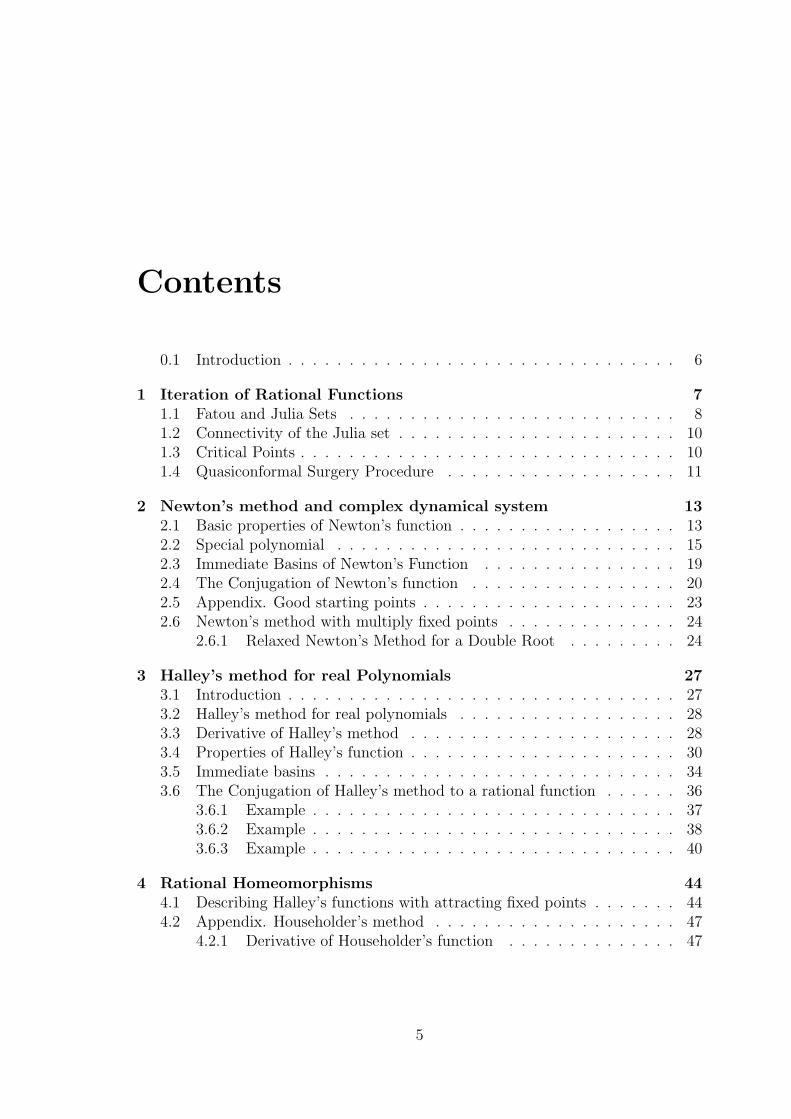
Suppose that d=5, then the special polynomial solution of the equation (2.2.7) existuniquely and is given by
p5(z) = a5z5 + a3z
3 + a1z, (2.2.11)
where a5 = ad = 1, by using the equation (2.2.10), we find that a3 = −107
and a1 = 37,
thus
p5(z) = z5 − 10
7z3 +
3
7z. (2.2.12)
50 100 150 200 250 300
50
100
150
200
250
300
Figure 2.4: Iteration of Newton’s function for the polynomial p5(z) = z5 − 107 z3 + 3
7z.

Newton’s method and complex dynamical system 19
Now consider d = 6, then the special polynomial solution takes the form
p6(z) = z6 − 5
3z4 +
5
7z2 − 1
21. (2.2.13)
50 100 150 200 250 300
50
100
150
200
250
300
Figure 2.5: Iteration of Newton’s function for the polynomial p6(z) = z6 − 53z4 + 5
7z2 − 121 .
Thus now we can find the special polynomial solution of the equation (2.2.7) forany degree, for example take a look at figure (2.6) and figure (2.7).
50 100 150 200 250 300
50
100
150
200
250
300
Figure 2.6: Iteration of Newton’s function for the polynomial p7(z) = z7 − 2111z5 + 35
33z3 − 533z,
where p7(z) is a polynomial solution of equation (2.2.7).

Newton’s method and complex dynamical system 20
50 100 150 200 250 300
50
100
150
200
250
300
Figure 2.7: Iteration of Newton’s function for the polynomial p8(z) = z8− 2813z6 + 210
143z4− 140429z2 +
5429 , where p8(z) is a polynomial solution of equation (2.2.7).
2.3 Immediate Basins of Newton’s Function
In this section, we want to show that each immediate basin of fixed points of New-ton’s function for a real polynomial is simply connected, so that we can apply the-orem (1.4.1) and we can use the quasiconformal surgery.
Theorem 2.3.1. Let
p(z) = adzd + ad−1z
d−1 + . . . + a1z + a0
be a polynomial with real coefficient and only real (and simple) zeros xk, 1 ≤ k ≤ d,and let (c1, c2) be a band containing xk and ζk (zero of p′′(x) which is a free criticalpoint), so the interval [xk, ζk] ⊂ (c1, c2). Then the interval between the fixed pointxk and free critical point ζk is mapped by N into itself, i.e. N [xk, ζk] ⊂ [xk, ζk].
Proof. We know that N(xk) = xk, N ′(xk) = 0, N ′(ζk) = 0, and we have to considertwo cases which are xk < ζk or xk > ζk. So let us start with the first case wherexk < ζk. In the previous section we have proved that
limx−→c+1
N(x) = +∞, limx−→c−2
N(x) = −∞.
Then from N(x) > xk in (c1, xk), it follows that
N(x) > xk in (xk, ζk), (2.3.1)
and since N(x) < ζk in (ζk, c2), then
N(x) < ζk in (xk, ζk), (2.3.2)

Newton’s method and complex dynamical system 21
from (2.3.1) and (2.3.2), it follows
N [xk, ζk] ⊂ [xk, ζk]. (2.3.3)
The second case is proved in the same manner. It also follows that ζk ∈ A∗(xk),where A∗(xk) is the immediate basin of attraction of xk.
Theorem 2.3.2. Let p(z) = adzd + ad−1z
d−1 + . . . + a1z + a0 be a polynomial withdistinct and real roots xk, 1 ≤ k ≤ d, and let N be Newton’s function associatedwith p(z). Then the immediate basin of each xk, 1 ≤ k ≤ d, is simply connected.
Proof. We know that xk, 1 ≤ k ≤ d, are superattracting fixed points, and ζk,2 ≤ k ≤ d− 1, are free critical points of Np(z). Let V = ∆(xk, ε) = {z : |z − xk| <ε} ⊂ A∗(xk), such that N(ζk) /∈ V . Let V1 be the component of N−1(V ) which
contains xk. Since ζk /∈ V1, it follows N : V12:1→ V , and by the Riemann Hurwitz
formula, it follows that V1 has the connectivity number n1 = 1. Let Vµ be thecomponent of N−µ(V ) which contains xk, let µ be the unique integer such thatN(ζk) ∈ Vµ and ζk /∈ Vµ, then Vµ is simply connected too. Since Vµ+1 contains
xk and ζk, N : Vµ+13:1→ Vµ has degree 3 with two critical points, by the previous
formula, it follows that Vi+1 has the connectivity number nµ+1 = 1. Since there isno more critical points in A∗(xk), thus A∗(xk) is simply connected.
2.4 The Conjugation of Newton’s function
In this section, we want to conjugate Newton’s function for p(z) to Newton’s functionfor a spacial polynomial which is a unique solution for the equation (2.2.7).
Theorem 2.4.1. Let N(z) be the Newton’s function associated with p(z), wherep(z) is a polynomial with distinct real (and simple) roots xk, 1 ≤ k ≤ d. Then N isquasiconformally conjugate to some function R with real superattracting fixed pointsxk, 1 ≤ k ≤ d, and R′(xk) = R′′(xk) = 0.
Remark 2.4.1. The proof will be based on theorem (1.4.1). We have to choose ψwhich is in theorem (1.4.1) to be symmetric with the real line. So when we apply ψon U all simple and real super-attracting fixed points will remain real.
Proof. (Theorem(2.4.1)). Now we have to apply theorem (1.4.1) on each simplyconnected component U of the Fatou set of our Newton’s function N . Since we haved − 2 basins, each one contains two critical points, one is a super-attracting fixedpoint xk, 1 ≤ k ≤ d, and the other one is a free critical point ζk, 2 ≤ k ≤ d−1. So byapplying above theorem d−2 times, and since ψ is symmetric with the real line theneach free critical point ζk, 2 ≤ k ≤ d−1 will be located at the super-attracting fixedpoint xk, 2 ≤ k ≤ d− 1. Thus we have a new rational function R having d distinctreal super-attracting fixed points, x1, x2, . . . , xd, with R′(xk) = R′′(xk) = 0.

Newton’s method and complex dynamical system 22
Note that the Julia set of R is the ψ-image of the Julia set of N , and the dynamicsof R outside ψ(U) are the same as those of N outside U .
Proposition 2.4.2. The rational function R which we get from theorem (2.4.1) is
the Newton’s function of some polynomial p =d∏
k=1
(z − xk).
Proof. Since z = x1, x2, . . . , xd and ∞ are fixed points of R with R′(xj) = 0, j =1, 2, . . . , d and R′′(xj) = 0, j = 2, 3, . . . , d− 1, R must be of the form
R(z) = z −(
d∑j=1
cj
z − xj
)−1
. (2.4.1)
Then after some elementary calculation we obtain
R′(x1) = 1− c1(x1 − x2)2(x1 − x3)
2 . . . (x1 − xd)2
[c1(x1 − x2)(x1 − x3) . . . (x1 − xd)]2.
But we have R′(x1) = 0, hence
c1(x1 − x2)2(x1 − x3)
2 . . . (x1 − xd)2
[c1(x1 − x2)(x1 − x3) . . . (x1 − xd)]2= 1,
which implies that c1 = 1. In the same way we can prove that cj = 1, for allj = 1, 2, . . . , d, thus
R(z) = z −(
d∑j=1
1
z − xj
)−1
. (2.4.2)
Now its easy to see that
(d∑
j=1
1
z − xj
)−1
=
(p′
p
)−1
,
wherep(z) = (z − x1)(z − x2) . . . (z − xd).
Then
R(z) = z − p(z)
p′(z),
which is Newton’s function of some polynomial p =d∏
k=1
(z − xk).
Proposition 2.4.3. Let R be as in theorem (2.4.1), associated with p(z) =d∏
k=1
(z −xk), then p is (up to normalization) the special polynomial of degree d.

Newton’s method and complex dynamical system 23
Proof. We know that R is Newton’s function associated with a polynomial p(z) ofdegree d with d distinct real zeros xk, 1 ≤ k ≤ d, and p′′ has d− 2 distinct real zerosxk, 2 ≤ k ≤ d− 1. Then it follows that
p′′(z)
p(z)(z − x1)(z − xd)
does not have any zero or pole, thus
p′′(z)
p(z)(z − x1)(z − xd) = constant = d(d− 1), (2.4.3)
andp′′(z)(z − x1)(z − xd)− d(d− 1)p(z) = 0. (2.4.4)
Now we can move the interval [x1, xd] to the interval [−1, 1] by using the followingtransformation
φ(x) =2x
xd − x1
+x1 + xd
x1 − xd
. (2.4.5)
So by the above transformation we can figure out a new polynomial p(z) 6≡ 0 whichsatisfy the following equation
p′′(z)(z2 − 1)− d(d− 1)p(z) = 0. (2.4.6)
This equation equals (2.2.7), and the polynomial solution is unique. If d is even,then
p(z) = zd +
d2∑
b=1
ad−2bzd−2b, (2.4.7)
and if d is odd, then
p(z) = zd +
d−12∑
b=1
ad−2bzd−2b, (2.4.8)
where
ad−2b = ai =(i + 2)(i + 1)ai+2
i(i− 1)− d(d− 1). (2.4.9)
Thus p is the normalized special polynomial of degree d.
Conclusion 1. Now we have conjugated Newton’s function for a real polynomialby a quasiconformal mapping to Newton’s function for a special polynomial. Sincewe have proved that each component of Fatou set of Np is simply connected, wehave also that all critical points of Np are located at the superattracting fixed pointsof Np. Thus the following theorem applies.
Theorem 2.4.4. ([Bea91] page 225) Suppose that the forward orbit of each criticalpoint of a rational function R accumulates at a (super)attracting cycle of R. ThenR is expanding on J.

Newton’s method and complex dynamical system 24
Now we can say that Np is expanding on J. On the other hand we can use thefollowing proposition.
Proposition 2.4.5. ([Ste93] page 118) If J ∩C+ = φ, then f is expanding on J , i.e.,there exist numbers δ > 0 and k > 1 such that
|(fn)′(z)| ≥ δkn
for n = 1, 2, . . . and z ∈ J .
Applying the following.
Theorem 2.4.6. ([Mil99] page 191) If the Julia set of a hyperbolic map is connectedthen it is locally connected.
Implies that Julia set of Np is locally connected.
2.5 Appendix. Good starting points
It is a fundamental problem to find all roots of a complex polynomial p. Newton’smethod is one of the most widely known numerical algorithms for finding the rootsof complex polynomials. For most starting points of most polynomials, it does nottake to long to find good approximations of a root. But there are problems, sincethere are starting points which never converge to a root under iteration of Newton’smethod (for example all the points on the boundaries of the basins of all the roots).Therefore, we suggest good, in other word convenient, starting points to find all realroots of a polynomials of degree d with d distinct real roots. These good startingpoints are ζk, 2 ≤ k ≤ d − 1, where ζk are zeros of p′′(z), and that is because wehave proved that Nn(ζk) → xk. So we can describe the algorithm as follows:
1. If d is even, then we find the zeros of p(d−2)(z), where p(d−2)(z) is the derivativeof p(z), d−2 times. So they are two good starting points for iteration of Np(z)to find the two roots in the middle which are x d
2, x d
2+1. Then we find the zeros
of p(d−4)(z), so we get another two starting points for iteration of Np(z) tofind another two roots which are x d
2−1, x d
2+2. We keep going by the same steps
until we find the zeros of p′′(z), then we have two starting points for iterationof Np to find the two roots x2, xd−1. Now for the last two roots which arex1, xd, we can start the iteration of Np(z) with any points x < x1 to get theroot x1, and with any point x > xd to get the root xd.
2. If d is odd, then we find the zero of p(d−1)(z), so it will be a good starting pointfor iteration of Np(z) to find the middle root which is x d+1
2. Then we find the
zeros of p(d−3)(z), so we get another two starting points for iteration of Np(z)to find the two roots which are x d−1
2, x d+3
2. Now we follow the same steps until
we find the zeros of p′′(z), then we have two starting points for iteration ofNp to find the two roots x2, xd−1. Finally for the two roots x1, xd, we can findthem as in case one.

Newton’s method and complex dynamical system 25
2.6 Newton’s method with multiply fixed points
In this section, we are enthusiastic in studying the dynamics of Newton’s functionof polynomial with multiply real zeros.
Remark 2.6.1. Let p(z) =d∏
i=1
(z − xi)ni , then Np(z) has the following properties:
(i) The points xi are (super)attracting fixed points with multipliers ni−1ni
, and whenni = 1 the local degree of Np at xi is at least 2.
(ii) The point ∞ is a repelling fixed point with multiplier dd−1
.
2.6.1 Relaxed Newton’s Method for a Double Root
In this subsection, we have a polynomial p of degree d, and there is one doubleroot. Then we have to prove that the immediate basin of a double root is simplyconnected and to do that, we first prove the following proposition.
Proposition 2.6.1. Let aj be the only double real root of p, and let the other rootsbe real and simply roots. Then the interval [µj, ζj] is mapped into itself, Np[µj, ζj] ⊂[µj, ζj], where µj, ζj are two free critical points belonging to the immediate basin ofaj.
Proof. Assume that µj < ζj, we know that N(aj) = aj, N ′(µj) = 0, N ′(ζj) = 0, andin the previous section, we have proved that
limx−→c+1
N(x) = +∞, limx−→c−2
N(x) = −∞.
Then from N(x) > µj in (c1, µj), it follows that
N(x) > µj in (µj, ζj), (2.6.1)
and since N(x) < ζj in (ζj, c2), it follows that
N(x) < ζj in (µj, ζj). (2.6.2)
From (2.6.1) and (2.6.2) we obtain
N [µk, ζj] ⊂ [µj, ζj]. (2.6.3)
It also follows that µj, ζj ∈ A∗(aj), where A∗(aj) is the immediate basin of attractionof aj.
Theorem 2.6.2. Let aj be as in proposition (2.6.1), then the immediate basin of aj
is simply connected.

Newton’s method and complex dynamical system 26
Figure 2.8:
Proof. The idea of this proof is the same as it is in the proof of theorem (2.3.2).But we have to note that, in this case the fixed point aj of N is not critical point,and we also have to keep in mind that aj has two preimages.
Hence we can conjugate Np to Np1 of degree d− 1 and p1 has d− 1 real (simple)roots, it follows that Np1 can be conjugated to Np, where p is a special polynomial.Thus we obtain the same conclusion (1).
Remark 2.6.2. By starting with an initial approximation z0 sufficiently close to aroot of p, if the root is simple, the sequence of iterates zk+1 = N(zk), will convergequadratically to the root. But if the root is a multiple one, the convergence is onlylinear [Pei89].
Remark 2.6.3. If p(z) is known to have a multiple of order exactly m, then applyNewton’s method to m
√p(z) to obtain
Nm(z) = z − p(z)1m
1m
p(z)1m−1p′(z)
= z − mp(z)
p′(z). (2.6.4)
This is called Newton’s method for a root of order m or the relaxed Newton’s method.This relaxed Newton’s method will converge quadratically to a root of order m.
(William J. Gilbert) [Wal48] using the above remarks in order to prove thefollowing theorem.
Theorem 2.6.3. The relaxed Newton’s method, N2 for a double root, applied to anycubic equation with a double root is conjugate, by a linear fractional transformationon the Riemann sphere, to the iteration of the quadratic p(z) = z2 − 3
4.
Newton’s method and complex dynamical system 27
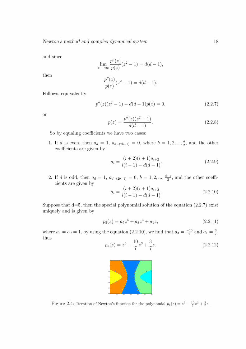
Example 1. Let
p(z) = (z + 2)2(z + 1)3z4(z − 1)2(z − 2)2(z − 3)3.
Since we have in this case n − 2 simply connected immediate basins, where n is
Figure 2.9: Newton’s function for the polynomial p(x) = (x+2)2(x+1)3x4(x−1)2(x−2)2(x−3)3.
the number of the roots, each one contains two free critical points and an attractingfixed point. So by applying theorem (1.4.1), n− 2 times and follow the same stepsin section (2.4). We will come with a new rational function R, and that R is aNewton’s function (as we have proved in proposition (2.4.2)), for a polynomial p1(z)with only real (and simply) zeros aj, j = 1, 2, . . . , n. Then we will have the samesituation as we mentioned before. Thus we can conjugate Newton’s function for p1
to the Newton’s function for a unique polynomial solution of the equation
p′′(z)(z2 − 1)− n(n− 1)p(z) = 0. (2.6.5)
But the problem is we can not study the general form of multiplicities because itsin general not known.
Note that the degree of Newton’s function for a polynomial of degree d, withmultiple roots will go down and equal to the number of the roots without multiplicity.

Chapter 3
Halley’s method for realPolynomials
3.1 Introduction
Halley’s method is an elegant method for finding roots. There are two methodscalled Halley’s method, one is called the irrational method and the other is calledrational method. The rational method is simpler and has some advantages over theirrational method since the latter involves taking the square root. And since thisthesis concerned with Halley’s rational method, then we will talk about Halley’smethod as a Halley’s rational method.Whereas Newton’s method is second order, we will show that Halley’s method is athird-order algorithm. Such an algorithm converges cubically insofar as the numberof significant digits eventually triples with each iteration. And not only does thefirst derivative of a third-order iteration vanish at a fixed point, but so does thesecond derivative.We can derive Halley’s method by using a second-degree Taylor approximation
R(x) ≈ R(xn) + R′(xn)(x− xn) +R′′(xn)
2(x− xn)2,
where xn is again an approximate root of R(x) = 0. As for Newton’s method, thegoal is to determine a point xn+1 where the graph of R intersects the x-axis, thatis, to solve the equation
0 = R(xn) + R′(xn)(xn+1 − xn) +R′′(xn)
2(xn+1 − xn)2, (3.1.1)
for xn+1. Following Frame [S.44] and others, we factor xn+1 − xn from the last twoterms of (3.1.1) to obtain
0 = R(xn) + (xn+1 − xn)
(R′(xn) +
R′′(xn)
2(xn+1 − xn)
),
28

Halley’s method for real Polynomials 29
from which it follows that
xn+1 − xn = − R(xn)
R′(xn) + R′′(xn)2
(xn+1 − xn). (3.1.2)
Approximating the difference xn+1 − xn remaining on the right-hand side of (3.1.2)
by Newton’s correction xn+1 − xn = − R(xn)R′(xn)
, we obtain
xn+1 = xn − 2R(xn)R′(xn)
2R′(xn)2 −R(xn)R′′(xn), (3.1.3)
which is widely known as Halley’s method.Note that Bateman [H38] was the first to point out that Halley’s method for a
function f(z) is obtained by applying Newton’s method to f(z)√f ′(z)
in the sense that
N f(z)√f ′(z)
(z) = z −f(z)√f ′(z)
( f(z)√f ′(z)
)′= Hf (z) for all z.
3.2 Halley’s method for real polynomials
In this section, our objective is to study the iteration of Halley’s function associatedwith a polynomial p of degree d with real coefficients and only real (and simple)zeros xk, 1 ≤ k ≤ d. This method is equivalent to iterating the rational map
Hp(z) = z − 2p′(z)p(z)
2(p′(z))2 − p(z)p′′(z), (3.2.1)
wherep(z) = a0 + a1z + a2z
2 + ... + ad−1zd−1 + adz
d.
So if p(z) has degree d and has distinct roots, then by a simple calculation Hp(z) isa rational map of degree 2d − 1. As for the case of Newton’s method, the roots ofp(z) are fixed points of Hp(z), although other fixed points exist as well. Since weare assuming that the roots of p(z) are distinct, the critical points of p(z) are alsofixed points under Halley’s method.
3.3 Derivative of Halley’s method
The derivative of Halley’s method is
H ′p(z) = − (p(z))2S[p](z)
2(p′(z)− p(z)p′′(z)
2p′(z)
)2 , (3.3.1)

Halley’s method for real Polynomials 30
where S[p](z) is the Schwarzian derivative of p(z), that is
S[p](z) =p′′′(z)
p′(z)− 3
2
(p′′(z)
p′(z)
)2
. (3.3.2)
From expression (3.3.1), we can see that the roots are super-attracting fixed points,but of one degree higher order than for Newton’s method.As we know that the degree of Halley’s function is 2d − 1, where d is the degreeof the polynomial p, there are 4d − 4 critical points, 2d of them coincide with theroots xk, and 2d − 4 are free critical points placed at points where the Schwarzianderivative of p(z) vanishes.
Remark 3.3.1. The second derivative of Hp vanishes at xk, where as the secondderivative of Np does not, the graph of Hp is flatter than that of Np near the fixedpoint. This accounts for the difference in speed at which the two algorithms converge(see [ST95], [E.49] for details). In general, the higher the order, the flatter thegraph, the faster convergence.
Figure 3.1: Halley’s function for the polynomial p(x) = x3 − x.

Halley’s method for real Polynomials 31
3.4 Properties of Halley’s function
Remark 3.4.1. Kœnig gave in [BH03] the general iteration
zn+1 = zn + (α + 1)
((1
p)(α)
(1p)(α+1)
),
where α is an integer and (1p)(α) is the derivative of order α of the inverse of the
polynomial p. This iteration has convergence of order (α + 2). For example α = 0has quadratic convergence (order 2) and the formula gives back Newton’s iteration,while α = 1 has cubical convergence (order 3) and gives again Halley’s method. Justlike Newton’s method, a good starting point is required to insure convergence.
Proposition 3.4.1. Let p : C −→ C be a polynomial of degree d with real coefficientsand real (and simple) zeros. Then:
1. Halley’s method associated with p is a rational map, it has a repelling fixedpoint at ∞ with multiplier d+1
d−1.
2. The local degree of Hp at the roots of p is exactly 3.
3. The rational map Hp has d−1 repelling fixed points in R and their multipliersare equal to 3.
Proof. (1) When |z| tends to ∞, we have
p(z) ∼ λzd,
( 1p(z)
)′ ∼ −dλzd+1 and ( 1
p(z))′′ ∼ d(d+1)
λzd+2 , we can write Hp in this form
Hp(z) = z + 2
(1
p(z)
)′(
1p(z)
)′′ ,
it follows
Hp(z) ∼ z − 2z
d + 1,
and
H ′p(z) ∼ d− 1
d + 1,
as we know that the multiplier λ at ∞ is equal to
limz−→∞
1
H ′p(z)
=d + 1
d− 1,
it follows that ∞ is a fixed point of Hp with multiplier d+1d−1
. This concludesthe proof of (1).

Halley’s method for real Polynomials 32
(2) The zeros of p are double critical points. Assume Ui = {z : |z − xi| < ε}is contained in A∗(xi), such that Ui does not contain Hp(z0), where z0 is afree critical point. Then from (3.3.1) and theorem (3.4.3) which show thatS[p](z) < 0, it follows that Ui contains exactly two critical points located atxi. Let Ui+1 be a component of H−1
p (Ui) contains xi. Then by using theRiemann Hurwitz Formula on Ui, Ui+1 we will find the degree of Hp equals 3on Ui, then The local degree of Hp at the roots of p is exactly 3.
(3) Let xi, i = 1, 2, · · · , d, be the zeros of p which are real and simple. The fixedpoints of Hp are ∞, the points xi and the zeros of the rational map g = (1
p)′,
where Hp written in the following form
Hp(z) = z + 2(1
p)′
(1p)′′
.
For any rational map, the number of zeros is equal to the number of poles.The poles of g are the points xi, and g has a zero of order d + 1 at ∞, thusg has 2d poles, it follows that g has 2d− (d + 1) = d− 1 zeros, consequently,Hp has d− 1 repelling fixed points. For any rational map, the number of fixedpoints counted with multiplicities equal to the degree plus 1. As we knowin our case that the fixed points of Hp are real and simple, then there are dsuper-attracting fixed points, one repelling fixed point at ∞ and d−1 repellingfixed points in R. Therefore the degree of Hp is 2d− 1.Now we have
Hp(z) = z +2g
g′,
where g = (1p)′. Thus
H ′p(z) = 3− 2gg′′
g′2,
and at the repelling fixed points p′ = 0 gives g = −p′p2 = 0. Thus H ′
p = 3 ateach repelling fixed point.
Theorem 3.4.2. Let
Hp(z) = z − 2p′(z)p(z)
2(p′(z))2 − p(z)p′′(z),
where p is a polynomial with real (and simply) distinct zeros. Then Hp has no realpole.
Proof. We will show that
(p′)2 − pp′′ > 0 on R,

Halley’s method for real Polynomials 33
which is known as Polya’s result.Write
(p′)2 − pp′′ = p2 (p′)2
p2− p2pp′′
p2= p2
((p′
p
)2
− p′′
p
).
We know that (p′
p
)2
=
(d∑
j=1
1
z − xj
)2
,
where xj are roots of p, 1 ≤ j ≤ d, hence
p′′
p=
(d∑
j=1
1
z − xj
)2
−d∑
j=1
1
(z − xj)2.
Fromd∑
j=1
1
(z − xj)2> 0, z ∈ R,
it follows that (p′
p
)2
>p′′
p,
hence2(p′)2 − pp′′ > 0.
Thus Hp does not have any real pole.
Theorem 3.4.3. Let Hp(z) be a Halley’s function for a polynomial p(z), thenH ′
p(z) ≥ 0 on R.
Proof. We know that
H ′p(z) = − (p(z))2S[p](z)
2(p′(z)− p(z)p′′(z)
2p′(z)
)2 ,
where S[p](z) is the Schwarzian derivative of p(z), that is
S[p](z) =p′′′(z)
p′(z)− 3
2
(p′′(z)
p′(z)
)2
=2p′p′′′ − 3(p′′)2
2(p′)2.
To show that H ′p(z) ≥ 0, we have to prove that S[p](z) < 0. By the same proof as
before, we can see that (p′′)2− p′p′′′ > 0, then 2p′p′′′− 3(p′′)2 < 0. Thus S[p](z) < 0,implies H ′
p(z) ≥ 0.
Conclusion 2. From theorems (3.4.2) and (3.4.3), we conclude that Hp is an in-creasing rational homeomorphism map on R.

Halley’s method for real Polynomials 34
Figure 3.2: Halley’s function for the polynomial p(x) = x6 − 53x4 + 5
7x2 − 121 .
50 100 150 200 250 300
50
100
150
200
250
300
Figure 3.3: Iteration of Halley’s function for the polynomial p(z) = z6 − 53z4 + 5
7z2 − 121 .

Halley’s method for real Polynomials 35
3.5 Immediate basins
We can not follow the same steps in the part of Newton’s method to prove thateach component of the Fatou set of Halley’s method is simply connected, becausein Halley’s method the free critical points are non-real numbers, so we can not workon the real line. But results in [Prz89] can be used to prove the immediate basinsof a superattracting fixed points of Halley’s method are simply connected.
Lemma 3.5.1. ( [Prz89]) Let A be the immediate basin of attraction to a fixedpoint for a rational map R : C −→ C. Assume that A is not simply connected.Then there exist in C two disjoint domains U0 and U1 intersecting A, such thatV = R(U0) = R(U1) ⊃ U0 ∪ U1, R(∂Ui) = ∂V ⊂ A for i = 0, 1, V ∪ A = C and Vis homeomorphic to a disc.
Theorem 3.5.2. The immediate basins of attraction to the roots of any polynomialwith real coefficients and only real (and simply) zeros xk, 1 ≤ k ≤ d, for Halley’smethod, are simply connected.
Proof. In [Prz89] Feliks Przytycki has proved that the immediate basins of attrac-tion for Np is simply connected. We can apply the same proof, so we can assume thatA is a multiply connected immediate basin of attraction for R = Hp to a root x ∈ Rof a polynomial p. Choose z ∈ V ∩A, V given by Lemma (3.5.1), and branches R−1,so that wi = R−1(z) ∈ Ui ∩A. Join z with wi by a curve γ0
i ⊂ V ∩A. Take care ad-ditionally to have γ0
i ∩ cl(⋃
n>0
Rn(critR)) = φ. Define by induction γni = R−1(γn−1
i ),
where R−1 is the extension of the preliminary branch along the curven−1⋃j=0
γji . Define
γi =∞⋃
n=0
γni . The curve γi converges to a fixed point ζi ∈ Ui of R. The reason is that
R−1vi◦ . . . ◦ R−1
vi, n times, n = 0, 1, . . . , is a normal family of functions on a neigh-
borhood of γi with the set of limit functions on boundary of A which is nowheredense. So all limit functions are constant, hence lim
n→∞diam(γn
i ) = 0. Therefore all
limit points of the sequence of curves γni are fixed points for R. On the other hand
they must be isolated from each other. So we actually have only one limit point.The conclusion is that the boundary of A contains two different fixed points ζ0, ζ1
belonging to two different components of the boundary of A. But the only fixedpoints for Hp are the roots of p (real), the roots of p′ (real), and ∞. Since we haveproved that Hp is continuous on R. Thus A ∩ R is an interval. We arrived at acontradiction.
Theorem 3.5.3. ( [Pom86]) Let ζ 6= ∞ be a repelling fixed point of some rationalfunction f . For µ = 1, 2, . . . ,m, let Gµ be different simply connected invariantcomponents of F (f), let hµ map D conformally onto Gµ, and let σµv be distinct fixedpoints of ϕµ = h−1
µ ◦ f ◦ hµ with
hµ(σµv) = ζ for v = 1, . . . , qµ.

Halley’s method for real Polynomials 36
Thenm∑
µ=1
qµ∑v=1
1
log ϕ′µ(σµv)
≤ 2
log |f ′(ζ)| .
Let A∗(xk), where k = 1, 2, . . . , d be different simply connected invariant com-ponents of F (Hp), Hp has d− 1 repelling fixed points on R with multiplier equal to3, then Gk = A∗(xk), let hk map D conformally onto A∗(xk), and let σkv be distinctfixed points of ϕk = h−1
k ◦Hp ◦ hk with
hk(σkv) = ζ for v = 1, . . . , m,
where ζ 6= ∞ is repelling fixed point of Hp. So from the above theorem we can provethe following theorem.
Theorem 3.5.4. Let p(z) be a polynomial of degree d ≥ 2 with real coefficients andonly real (and simply) zeros, Hp(z) be the Halley’s function associated with p(z), andA∗(x1), A
∗(x2), . . . , A∗(xd) are the immediate basins of superattracting fixed points
of Hp(z). Then there are at least two free critical points in each second immediatebasin.
Proof. Denote by x1, x2, . . . , xd−1, xd the d superattracting fixed points of Hp(z). Weknow that each immediate basin A∗(xi), 1 ≤ i ≤ d, is simply connected and thelocal degree of Hp at each xi is exactly 3. Now take A∗(xi), A
∗(xi+1) and assumethat both of them do not contain any free critical points; then the degree of Hp(z)in both basins is equal to 3. It follows that there exists a conformal representationh−1 : A∗(xk) −→ D, k = i, i + 1, conjugating Hp : A∗(xk) −→ A∗(xk) to themapping ϕk : D → D, where the degree of ϕk is exactly 3. Then there are at leasttwo external rays which land at ζ, where ζ ∈ (xi, xi+1) is a repelling fixed point ofHp. By the inequality in theorem (3.5.3), we get
i+1∑
k=i
m∑v=1
1
log ϕ′k(σkv)
<2
log |H ′(ζ)| =2
log 3.
Since ϕk = h−1k ◦Hp ◦ hk with
hk(σkv) = ζ for v = 1, . . . , m,
and H ′p(ζ) = 3, it follows that ϕ
′k(σkv) = 3, and
2m
log 3<
2
log 3.
Then we get a contradiction because m ≥ 2. Therefore if the degree of Hp(z) inA∗(xi) equals 3, then the degree of Hp in A∗(xi+1) must be ≥ 5. Since it is odd,then each second immediate basin of superattracting fixed point contains at leasttwo free critical points.
Halley’s method for real Polynomials 37
Proposition 3.5.5. If polynomials p, p have Halley’s functions Hp, Hp which areconformal conjugate, i.e. Hp = ϕ−1 ◦Hp ◦ ϕ(z), then p(z) = c p(ϕ(z)), where c is aconstant.
Proof. Consider ϕ(z) = az + b, then ϕ−1(z) = z−ba
, and we can write Halley’sfunction as follow
Hp = z + 2g
g′,
where g = (1p)′ and g′ = (1
p)′′, by simple calculation we have
Hp(z) = z + 2g(ϕ(z))
ag′(ϕ(z)),
so it follows thatg(z)
g′(z)=
g(ϕ(z))
ag′(ϕ(z)),
we have a = ϕ′(z) then
log g(z) = log g(ϕ(z)) implies g(z) = c g(ϕ(z)).
Thusp(z) = c p(ϕ(z)).
3.6 The Conjugation of Halley’s method to a ra-
tional function
Since all free critical points of Hp(z) are complex numbers, we can not prove directlythat each A∗(xk) contains exactly four critical points, that is, that the degree ofHp(z) on A∗(xk) is exactly equal to 5. We also do not know that Hp is hyperbolic.But we can look for a rational map R(z) which satisfies the following conditions:degR(z) = degHp(z), and R(z) has d real superattracting fixed points, with propertythat all the critical points of R(z) are located at the superattracting fixed points ofR(z). Now we consider the following three subsections as examples to find rationalmaps R3, R4, R5 with the above conditions and property, so that we can conjugateHalley’s function Hpd
, where d = 3, 4, 5 is the degree of p, to the rational map Rd.For simplification, we will consider pd(z) to be the special polynomials of degreed = 3, 4, 5.

Halley’s method for real Polynomials 38
50 100 150 200 250 300
50
100
150
200
250
300
Figure 3.4: Iteration of Halley’s function for the polynomial p3(z) = z3 − z.
3.6.1 Example
In this subsection, we explore the dynamics of Halley’s method applied to cubicpolynomials (p3) with real coefficients and only real (and simply) zeros xk, k = 1, 2, 3.Consider p3 a special polynomial of degree three
p3(z) = (z − 1)(z + 1)z.
Then the Schwarzian derivative S[p3](z) vanishes at ρ± = ± i√6, which are the two
free critical points. Note that in this example, the free critical points of Halley’smethod are symmetric about the free critical points of Newton’s method, here wealso have that Re(ρ−) = Re(ρ+) = 0. Since its easy to see that Hp3(iR) ⊆ iR and0 ∈ iR, therefore iR ⊂ A∗(0) (the immediate basin of attraction for Hp3 to the rootz = 0 of p3), then ρ± ∈ A∗(0), which means that ρ± converge to zero under iterationof Hp3 . So we then have two critical points at a root z = 1, two critical points at aroot z = −1, and the other four critical points belong to A∗(0), two of them are atthe root z = 0. So we are now looking for a rational map R3(z) which satisfy theseconditions:degR3(z) = 5, R3(±1) = ±1, R3(0) = 0, R′
3(0) = 0, R′3(±1) = 0, R′′
3(0) = 0,
R′′3(±1) = 0, R
(3)3 (0) = 0, and R
(4)3 (0) = 0.
By using Maple with the above conditions, we found a rational map
R3(z) =8z5
15z4 − 10z2 + 3,

Halley’s method for real Polynomials 39
with degR3 = degHp3 and it has the same fixed points of Hp3 which are 0, 1,−1,±0.654(approximately), and ∞, where the critical points of R3(z) are
0, 0, 0, 0, 1, 1,−1,−1.
By theorem (1.2.3), J(Hp) is connected. Since A∗(0) contains a pair of free critical
Figure 3.5: Rational function R3(x).
points, it follows P (Hp3)∩J(Hp3) = φ. Thus Hp3 is hyperbolic and J(Hp3) is locallyconnected. Hp3 is quasiconformally conjugate to R3 with 3 superattracting fixedpoints and all critical points located at these fixed points.
3.6.2 Example
We want to study the dynamics of Halley’s method applied to polynomials of degreefour with real coefficients and real (and simple) zeros xk, k = 1, 2, 3, 4. Let p4 bethe special polynomial of degree four
p4(z) = (z2 − 1)(z2 − 1/5),
the zeros of p4 are±1,± 1√5
and the zeros of p′4 are 0, and approximately±0.7745966,they are fixed points of Hp4 . Since
Hp4(z) = z − 2p′4(z)p4(z)
2(p′4(z))2 − p4(z)p′′4(z),
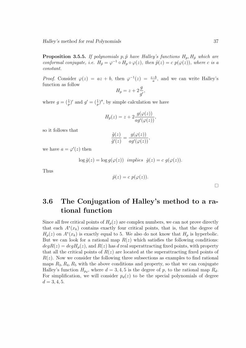
Halley’s method for real Polynomials 40
Figure 3.6: Halley’s function for the special polynomial of degree four (Hp4(x)).
and
H ′p4
(z) = − (p4(z))2S[p](z)
2(p′4(z)− p4(z)p′′4 (z)
2p′4(z))2
,
there are two critical points at each zero of p4(z). In total we have 12 criticalpoints, thus there are 4 free critical points, where the Schwarzian derivative S[p4](z)vanishes; these zeros are approximately equal to ±0.4406405322 ± 0.2723308257i.Now we have to look for a rational map R4(z) which satisfies the following conditions:degR4(z) = 7, R4(±1) = ±1, R4(0) = 0, R4(± 1√
5) = ± 1√
5, and
R′4(±
1√5) = R′
4(±1) = R′′4(±1) = R′′
4(±1√5) = R
(3)4 (± 1√
5) = R
(4)4 (± 1√
5) = 0.
Again by using Maple we found the following rational map
R4(z) =225z7 − 195z5 + 11z3 + 23z
350z6 − 430z4 + 138z2 + 6.
So we now have a rational map R4(z) with degR4(z) = degHp4(z) and R4(z) hassuperattracting fixed points±1,± 1√
5and repelling fixed points 0 and±0.8246211251
(approximately) with multiplier approximately equal to λ = 3.36. The interestingthing about properties of R4(z) is that all of its critical points are
1, 1,−1,−1,1√5,
1√5,
1√5,
1√5,− 1√
5,− 1√
5,− 1√
5,− 1√
5,
Halley’s method for real Polynomials 41
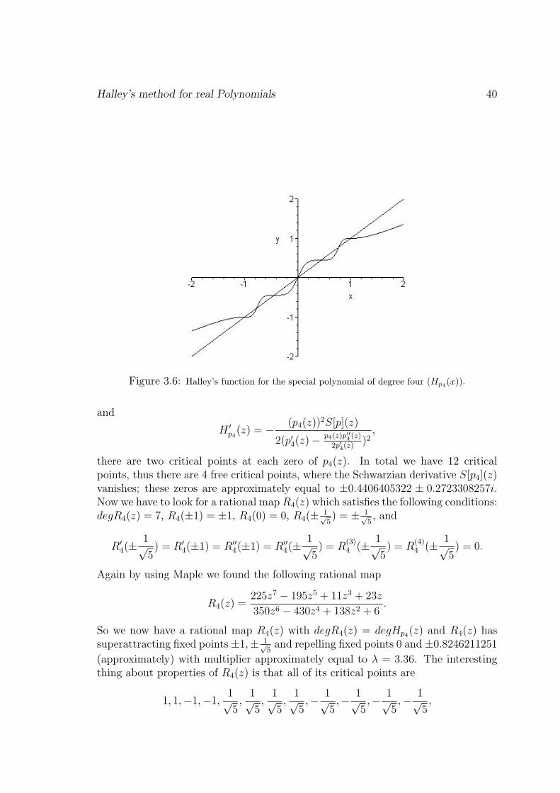
which means that all the critical points are located at the superattracting fixedpoints of R4(z). Now since each immediate basin A∗(xk) is simply connected, thusjulia set of Hp4 is connected. If each A∗(xk) contains a pair of free critical points, itfollows P (Hp4)∩J(Hp4) = φ. Thus Hp4 is hyperbolic and J(Hp4) is locally connected,and Hp4 is quasiconformally conjugate to R4.
Figure 3.7: Iteration of Halley’s function for the polynomial p4(z) = (z2 − 1)(z2 − 1/5).
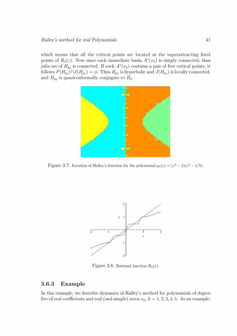
Figure 3.8: Rational function R4(x).
3.6.3 Example
In this example, we describe dynamics of Halley’s method for polynomials of degreefive of real coefficients and real (and simple) zeros xk, k = 1, 2, 3, 4, 5. As an example,
Halley’s method for real Polynomials 42
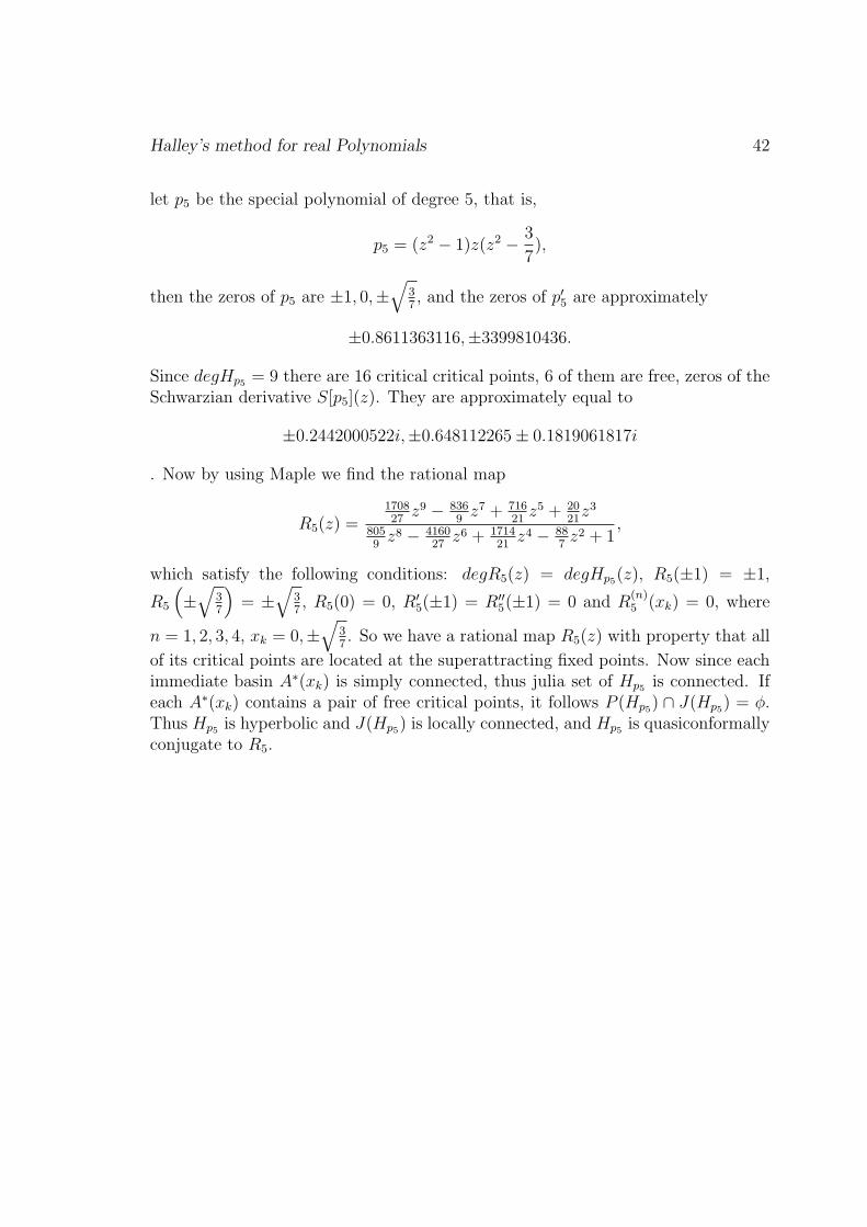
let p5 be the special polynomial of degree 5, that is,
p5 = (z2 − 1)z(z2 − 3
7),
then the zeros of p5 are ±1, 0,±√
37, and the zeros of p′5 are approximately
±0.8611363116,±3399810436.
Since degHp5 = 9 there are 16 critical critical points, 6 of them are free, zeros of theSchwarzian derivative S[p5](z). They are approximately equal to
±0.2442000522i,±0.648112265± 0.1819061817i
. Now by using Maple we find the rational map
R5(z) =170827
z9 − 8369
z7 + 71621
z5 + 2021
z3
8059
z8 − 416027
z6 + 171421
z4 − 887z2 + 1
,
which satisfy the following conditions: degR5(z) = degHp5(z), R5(±1) = ±1,
R5
(±
√37
)= ±
√37, R5(0) = 0, R′
5(±1) = R′′5(±1) = 0 and R
(n)5 (xk) = 0, where
n = 1, 2, 3, 4, xk = 0,±√
37. So we have a rational map R5(z) with property that all
of its critical points are located at the superattracting fixed points. Now since eachimmediate basin A∗(xk) is simply connected, thus julia set of Hp5 is connected. Ifeach A∗(xk) contains a pair of free critical points, it follows P (Hp5) ∩ J(Hp5) = φ.Thus Hp5 is hyperbolic and J(Hp5) is locally connected, and Hp5 is quasiconformallyconjugate to R5.
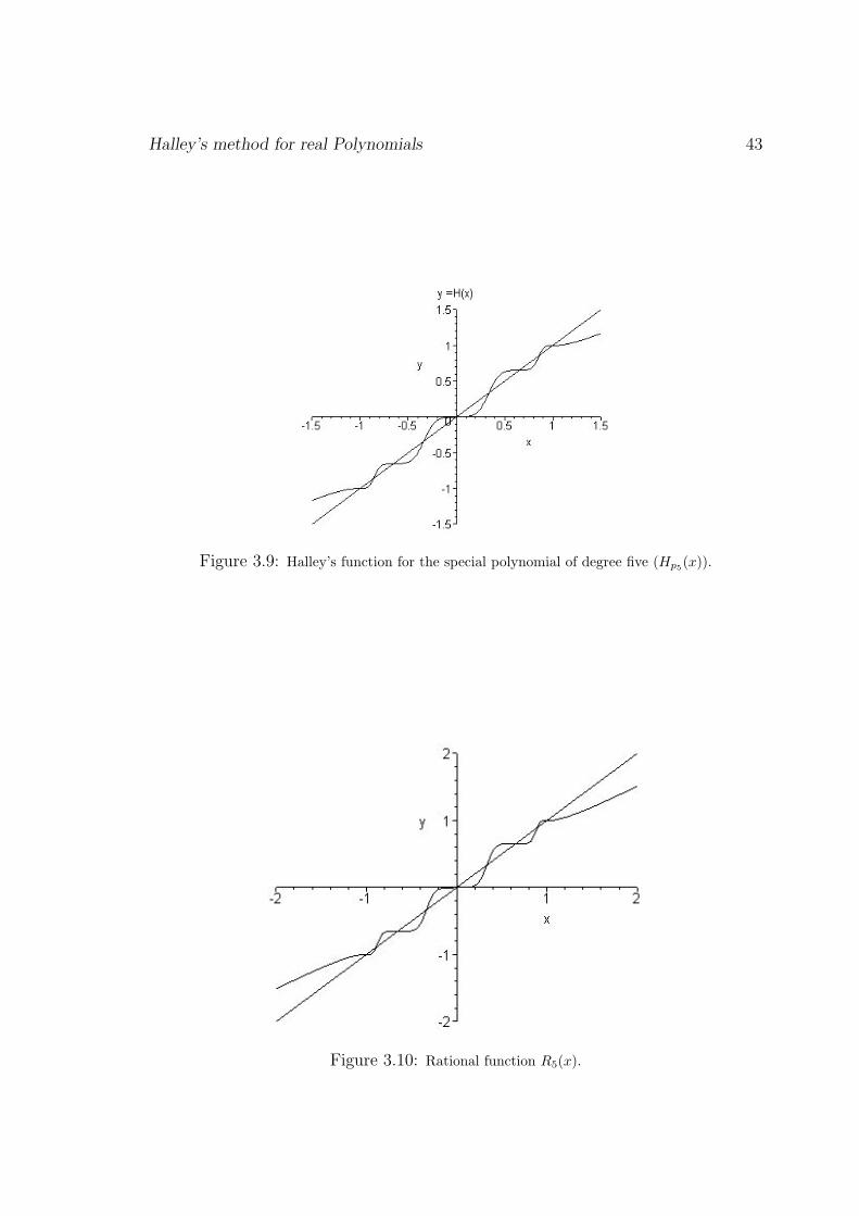
Halley’s method for real Polynomials 43
Figure 3.9: Halley’s function for the special polynomial of degree five (Hp5(x)).
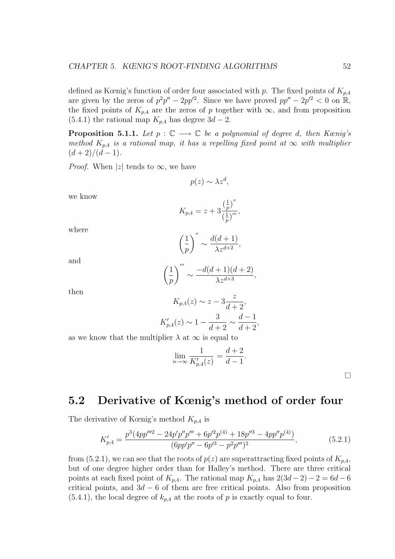
Figure 3.10: Rational function R5(x).

Halley’s method for real Polynomials 44
50 100 150 200 250 300
50
100
150
200
250
300
Figure 3.11: Iteration of Halley’s function for the polynomial p5(z) = (z2 − 1)z(z2 − 37 ).

Chapter 4
Rational Homeomorphisms
In this section, we want to describe the dynamics of the iterates of the familyA ={Rational maps which are homeomorphism on R and all fixed points ∈ R∪∞}.Since we have shown in the previous chapter that Hp (Halley’s function for poly-nomial with real coefficients and only real (and simple) zeros) is a homeomorphismrational map, then its a subset of A. Note that Hp has a superattracting fixedpoints at the zeros of p, that is the multiplier (λ = 0), and the repelling fixed pointsat the zeros of S[p] (Schwarzian derivative), so by elementary calculation we foundthat at the repelling fixed points of Hp the multiplier (λ = 3), then Hp would bea good example to describe dynamics of a homeomorphism rational maps R ⊂ A,where all the fixed points of R are superattracting, or repelling, that is, λ = 0, λ > 1.
4.1 Describing Halley’s functions with attracting
fixed points
We know that the class of Halley’s functions with real attracting fixed points belongto the family A. Now we want to study Halley’s method for a polynomial p ofdegree d with real zeros and some of them with multiplicity ≥ 2. We then obtainHalley’s function with some of its fixed points attracting fixed points, and somesuperattracting. Let
Hp(z) = z + 2(1
p)′
(1p)′′
.
If p of degree d has only real zeros, it follows that each root of p with multiplicity≥ 2 is an attracting fixed point of Hp.
Definition 4.1.1. The extraneous fixed points of Hp are the fixed points which arezeros of (1
p)′.
45

Homeomorphism Rational Maps 46
Lemma 4.1.1. Let p : C −→ C be a polynomial of degree d ≥ 2 with real zeros. Ifζ is a zero of (1
p)′ with multiplicity m, then it is a repelling fixed point of Hp with
multiplier (1 + 2m
).
Proof. We have
Hp(z) = z +2g(z)
g′(z)where g = (
1
p)′.
If ζ is a zero of g of order m, then there exists a λ ∈ C \ {0} such that
g(z) = λ(z − ζ)m + O(|z − ζ|m+1),
andg′(z) = λm(z − ζ)m−1 + O(|z − ζ|m).
Thus
Hp(z) = z +2λ(z − ζ)m
λm(z − ζ)m−1+ O(|z − ζ|2)
= ζ + z − ζ +2(z − ζ)
m+ O(|z − ζ|2)
= ζ + (z − ζ)(1 +2
m) + O(|z − ζ|2),
therefore, ζ is a repelling fixed point of Hp(z) and its multiplier is (1 + 2m
).
Remark 4.1.1. In the case of Newton’s Method for polynomial there are no extrane-ous fixed points, but as for Halley’s method case for a polynomial, the extraneousfixed points are the critical points of p which are not zeros of p.
Proposition 4.1.2. Let p be a real polynomial of degree d ≥ 2. Denote by xi,1 ≤ i ≤ d, its zeros and by ni their multiplicities. Then the fixed points of Hp areeither superattracting, attracting or repelling. The superattracting and attractingfixed points are exactly the zeros xi and their multipliers are 1− 2
ni+1, when ni = 1,
the local degree of Hp at xi equals at least 3.
Remark 4.1.2. From lemma (4.1.1), we know that the extraneous fixed points of Hp
are exactly the zeros of (1p)′. If ζj is a zero of (1
p)′ with multiplicity mj, then it is a
repelling fixed point of Hp with multiplier (1 + 2mj
).
Example 2. Considerp(z) = (z2 − 1)z3,
and
Hp(z) = z −2(1
p)′
(1p)′′
.
Then the superattracting fixed points of Hp are ±1 with multiplicity n = 1 andmultiplier λ = 1− 2
n+1= 1− 2
2= 0, the attracting fixed point is zero with multiplicity

Homeomorphism Rational Maps 47
n = 3 and multiplier λ = 1 − 23+1
= 12, and the repelling fixed points of Hp(z) are
the zeros of (1p)′ which are approximately equal to ±0.774596692 with multiplier
λ = 3. Moreover, p has N = 3 distinct real roots, then there are 4N − 4 = 8critical points of Hp(z) which are 1, 1,−1,−1, and four non-real free critical pointswhich are approximately equal to ±0.5460815697± 0.2195565548i. Now since eachimmediate basin is simply connected, then Julia set is connected. If A∗(0) containsthe four free critical points, then Hp is hyperbolic and J(Hp) is locally connected.We can also conjugate Hp(z), where p(z) = z5 − z3, to the rational function:
R3(z) =8z5
15z4 − 10z2 + 3,
which we have discussed in the previous chapter.
Figure 4.1: Halley’s function for the polynomial p(x) = x5 − x3.
50 100 150 200 250 300
50
100
150
200
250
300
Figure 4.2: Iteration of Halley’s function for the polynomial p(z) = z5 − z3.

Appendix. Householder’s method 48
4.2 Appendix. Householder’s method
Letp(z) = a0 + a1z + a2z
2 + · · ·+ ad−1zd−1 + adz
d,
be a polynomial with real coefficients and only real (and simple) zeros xk, 1 ≤ k ≤ d.The method is equivalent to iterating the rational map
hp(z) = z − 2p(z)(p′(z))2 + (p(z))2p′′(z)
2(p′(z))3, (4.2.1)
is called Householder’s method associated with p. So the fixed points of hp are givenby
2(p′(z))2p(z) + (p(z))2p′′(z)
2(p′(z))3= 0, or p(z)[2(p′(z))2 + p(z)p′′(z)] = 0.
Thus the fixed points of hp are the zeros of p at xk, 1 ≤ k ≤ d, the zeros of[2(p′(z))2 + p(z)p′′(z)] at x
′k, 1 ≤ k ≤ d, and at x
′′k, where 2 ≤ k ≤ d − 1, and ∞.
The degree of hp is 3d− 2, where d is the degree of p(z).
Definition 4.2.1. If c1 < c2 are consecutive roots of p′(x), then the interval (c1, c2)is called a band for hp.
Definition 4.2.2. If p′(x) has the largest (respectively, smallest ) root c (respec-tively, b ), then the interval (c,∞) (respectively, (−∞, b)) is called an extreme bandfor hp.
So in each band (ck, ck+1) which contains xk there are two repelling fixed pointsx′k, x
′′k and one superattracting fixed point xk, where 2 ≤ k ≤ d − 1, and there are
two fixed points in each extreme band.
4.2.1 Derivative of Householder’s function
Since
h′p(z) = −(p(z))2[p′(z)p′′′(z)− 3(p′′(z))2]
2(p′(z))4, (4.2.2)
we see that the zeros of p are superattracting fixed points of hp, and there are doublecritical points at each superattracting fixed point. The number of critical points is6d − 6, and 4d − 6 of them are free critical points which are non-real, so we are inthe same situation of Halley’s method. But in Householder’s method there are d−1poles as in Newton’s method. And there are 2d− 2 real repelling fixed points whichare the zeros of (2(p′(z))2 + p(z)p′′(z)).
Proposition 4.2.1. Let hp(z) be Householder’s function associated with p(z), wherep(z) is a polynomial with real coefficients and only real (and simple) zeros, thenh′p(z) ≥ 0 on each band (ck, ck+1), where 2 ≤ k ≤ d− 1.

Appendix. Householder’s method 49
Figure 4.3: Householder’s function for the polynomial p4(x) = (x2 − 1)(x2 − 15 ).
Proof. See (4.2.1). By Polya’s result we have
p′2 − pp′′ > 0 on R,
hence alsop′′2 − p′p′′′ > 0,
and this implies h′p(x) ≥ 0 on R except at zeros of p′.
Figure 4.4: Householder’s function for the polynomial p5(x) = x5 − 107 x3 + 3
7x.

Appendix. Householder’s method 50
Theorem 4.2.2. Immediate basins of attraction of the roots of polynomial with realcoefficients and only real (and simple) zeros xk, 1 ≤ k ≤ d, for the Householder’smethod are simply connected.
Proof. We know that in each band (ck, ck+1) there are two real repelling fixed pointswhich are zeros of 2p′2−pp′′. Let x
′k, x
′′k be two consecutive real repelling fixed points
of hp(z), then there exists a superattracting fixed point xk ∈ [x′k, x
′′k] ⊂ (ck, ck+1).
Now we want to show that [x′k, x
′′k] is mapped into itself under iteration of hp. We
have shown that h′p ≥ 0 on each band, hence hp(z) is increasing and continuous on
each band. So if x ≥ x′k then hp(x) ≥ x
′k, and if x ≤ x
′′k then hp(x) ≤ x
′′k. It follows
thathp[x
′k, x
′′k] = [x
′k, x
′′k].
ThusA∗(xk) ∩ [x
′k, x
′′k] = [x
′k, x
′′k].
Now since hp(x) is continuous on [x′k, x
′′k], we can follow the same path as in the proof
of theorem (3.5.2), which shows that each immediate basins of Halley’s method issimply connected.
Since there are free critical points which are non-real. Then we are in the samesituation of Halley’s method.

Chapter 5
Kœnig’s root-finding algorithms
In this chapter, we first recall the definition of a family of Kœnig’s root-findingalgorithms known as Kœnig’s algorithms (Kp,n) [BH03] for polynomials. In thewhole chapter p has degree d ≥ 2 with real coefficients and real (and simple) zerosxk , 1 ≤ k ≤ d. Now we want to discuss Kœnig’s algorithms in details where n = 4,(Kp,4(z)).
Definition 5.0.3. Let
p(z) = a0 + a1z + a2z2 + · · ·+ ad−1z
d−1 + adzd,
be a polynomial with real coefficients and real (and simple) zeros xk, 1 ≤ k ≤ d,and n ≥ 2 is an integer. Kœnig’s method of p of order n is defined by the formula
Kp,n(z) = z + (n− 1)(1
p)[n−2]
(1p)[n−1]
, (5.0.1)
where (1p)[n] is the nth derivative of 1
p.
For n = 2 the map Kp,n is Newton’s method of p, for n = 3 the map Kp,n isHalley’s method of p, and Householder’s method
hp(z) = Kp,2(z)− p
2p′K ′
p,2
which we have discussed all of them in the previous chapters.
5.1 Kœnig’s root-finding algorithms of order four
Let p be a polynomial with real coefficients and real (and simple) zeros xk, 1 ≤ k ≤ d,then
Kp,4 = z − 3p2p′′ − 2pp′2
6pp′p′′ − 6p′3 − p2p′′′, (5.1.1)
51
CHAPTER 5. KŒNIG’S ROOT-FINDING ALGORITHMS 52
defined as Kœnig’s function of order four associated with p. The fixed points of Kp,4
are given by the zeros of p2p′′ − 2pp′2. Since we have proved pp′′ − 2p′2 < 0 on R,the fixed points of Kp,4 are the zeros of p together with ∞, and from proposition(5.4.1) the rational map Kp,4 has degree 3d− 2.
Proposition 5.1.1. Let p : C −→ C be a polynomial of degree d, then Kœnig’smethod Kp,4 is a rational map, it has a repelling fixed point at ∞ with multiplier(d + 2)/(d− 1).
Proof. When |z| tends to ∞, we have
p(z) ∼ λzd,
we know
Kp,4 = z + 3(1
p)′′
(1p)′′′
,
where (1
p
)′′
∼ d(d + 1)
λzd+2,
and (1
p
)′′′
∼ −d(d + 1)(d + 2)
λzd+3,
thenKp,4(z) ∼ z − 3
z
d + 2,
K ′p,4(z) ∼ 1− 3
d + 2∼ d− 1
d + 2,
as we know that the multiplier λ at ∞ is equal to
limn→∞
1
K ′p,4(z)
=d + 2
d− 1.
5.2 Derivative of Kœnig’s method of order four
The derivative of Kœnig’s method Kp,4 is
K ′p,4 =
p3(4pp′′′2 − 24p′p′′p′′′ + 6p′2p(4) + 18p′′3 − 4pp′′p(4))
(6pp′p′′ − 6p′3 − p2p′′′)2, (5.2.1)
from (5.2.1), we can see that the roots of p(z) are superattracting fixed points of Kp,4,but of one degree higher order than for Halley’s method. There are three criticalpoints at each fixed point of Kp,4. The rational map Kp,4 has 2(3d− 2)− 2 = 6d− 6critical points, and 3d − 6 of them are free critical points. Also from proposition(5.4.1), the local degree of kp,4 at the roots of p is exactly equal to four.

CHAPTER 5. KŒNIG’S ROOT-FINDING ALGORITHMS 53
Remark 5.2.1. Let x be a simple zero of p, then Kp,4(x) = x and from (5.4.1)
K ′p,4(x) = K ′′
p,4(x) = K ′′′p,4(x) = 0, while K
(4)p,4(x) 6= 0. Thus Kp,4 is of order four
for simple roots. Since p(x) = 0, it follows that Np(x) = Hp(x) = Kp,4(x) = x,and this fixed point is superattracting fixed point for the three methods becauseN ′
p(x) = H ′p(x) = K ′
p,4(x) = 0. And since the third derivative of Kp,4 vanishes,whereas the third derivative of Hp does not, the graph of Kp,4 is flatter than thatof Hp near the fixed point. Thus Kp,4 is faster convergence to the fixed point thanHp. From figures (5.1,5.2), Kœnig’s function (Kp,4) looks like Newton’s function but(Kp,4), where p(z) = z3 − z, has non-real critical points whereas Newton’s functiondoes not.
Figure 5.1: Kœnig’s function for the polynomial p(x) = x3 − x.
Proposition 5.2.1. Let p : C→ C be a polynomial of degree d with real coefficientsand real (and simple) zeros. Then the rational map Kp,4 has 2d − 2 repelling fixedpoints in C and their multipliers are all equal to four.
Proof. Let
Kp,4(z) = z + 3g(z)
g′(z),
where
g = (1
p)′′
=2p′2 − pp′′
p3, (5.2.2)

CHAPTER 5. KŒNIG’S ROOT-FINDING ALGORITHMS 54
50 100 150 200 250 300
50
100
150
200
250
300
Figure 5.2: Iteration of Kœnig’s function for the polynomial p(z) = z3 − z.
g′ = (1
p)′′′
=6pp′p′′ − 6p′3 − p2p′′′
p4.
Let xk, 1 ≤ xk ≤ d, be the zeros of p which are real and simple. The fixed pointsof Kp,4(z) are ∞, the points xk and the zeros of the rational map g = (1
p)′′. From
(5.2.2), we can see that g has 3d poles. When z → ∞, then p(z) ∼ λzd and itfollows that g has a zero of order d + 2 at ∞. Since the number of zeros for anyrational map is equal to the number of poles, then g has 3d− (d + 2) = 2d− 2 finitezeros. Since we have proved that 2p′2− pp′′ > 0 on R, 2d− 2 zeros of g are non-realrepelling fixed points of Kp,4. Now we have
K ′p,4 = 4− 3gg′′
g′2,
and at the repelling fixed points of Kp,4, g = 0. Thus K ′p,4 = 4 at each repelling
fixed point.
Definition 5.2.1. If c1 < c2 are consecutive real poles of Kp,4, then the interval(c1, c2) is called a band for Kp,4.
Proposition 5.2.2. If (c1, c2) is a band for Kp,4 that contains a root of p(x), then
limx→c+1
Kp,4(x) = +∞, limx→c−2
Kp,4(x) = −∞.
Proof. From
Kp,4 = z − 3p(pp′′ − 2p′2)
6p′(pp′′ − p′2)− p2p′′′,
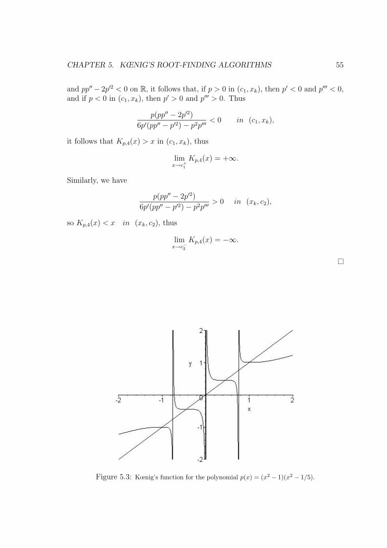
CHAPTER 5. KŒNIG’S ROOT-FINDING ALGORITHMS 55
and pp′′− 2p′2 < 0 on R, it follows that, if p > 0 in (c1, xk), then p′ < 0 and p′′′ < 0,and if p < 0 in (c1, xk), then p′ > 0 and p′′′ > 0. Thus
p(pp′′ − 2p′2)6p′(pp′′ − p′2)− p2p′′′
< 0 in (c1, xk),
it follows that Kp,4(x) > x in (c1, xk), thus
limx→c+1
Kp,4(x) = +∞.
Similarly, we have
p(pp′′ − 2p′2)6p′(pp′′ − p′2)− p2p′′′
> 0 in (xk, c2),
so Kp,4(x) < x in (xk, c2), thus
limx→c−2
Kp,4(x) = −∞.
Figure 5.3: Kœnig’s function for the polynomial p(x) = (x2 − 1)(x2 − 1/5).
CHAPTER 5. KŒNIG’S ROOT-FINDING ALGORITHMS 56
50 100 150 200 250 300
50
100
150
200
250
300
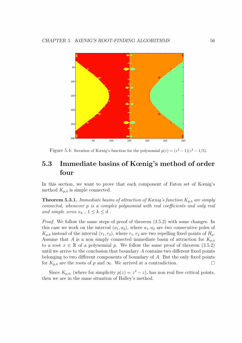
Figure 5.4: Iteration of Kœnig’s function for the polynomial p(z) = (z2 − 1)(z2 − 1/5).
5.3 Immediate basins of Kœnig’s method of order
four
In this section, we want to prove that each component of Fatou set of Kœnig’smethod Kp,4 is simple connected.
Theorem 5.3.1. Immediate basins of attraction of Kœnig’s function Kp,4 are simplyconnected, whenever p is a complex polynomial with real coefficients and only realand simple zeros xk , 1 ≤ k ≤ d .
Proof. We follow the same steps of proof of theorem (3.5.2) with some changes. Inthis case we work on the interval (a1, a2), where a1, a2 are two consecutive poles ofKp,4 instead of the interval (r1, r2), where r1, r2 are two repelling fixed points of Hp.Assume that A is a non simply connected immediate basin of attraction for Kp,4
to a root x ∈ R of a polynomial p. We follow the same proof of theorem (3.5.2)until we arrive to the conclusion that boundary A contains two different fixed pointsbelonging to two different components of boundary of A. But the only fixed pointsfor Kp,4 are the roots of p and ∞. We arrived at a contradiction.
Since Kp,4, (where for simplicity p(z) = z3− z), has non real free critical points,then we are in the same situation of Halley’s method.

CHAPTER 5. KŒNIG’S ROOT-FINDING ALGORITHMS 57
5.4 General form of Kœnig’s method
The following rational map
Kp,n(z) = z + (n− 1)(1
p)[n−2]
(1p)[n−1]
,
is the general form of Koing’s function. We end this chapter with some general re-marks describe, without proof, the dynamics of the general form of Kœnig’s functionKp,n. We will consider p be a special polynomial of degree d ≥ 2 which is a complexpolynomial with real coefficients and real (and simple) zeros xk, 1 ≤ k ≤ d, andp′(xk) = p′′(xk) = 0.
Proposition 5.4.1. Let p : C → C be a polynomial of degree d ≥ 2. Then for anyn ≥ 2,
(a) The rational map Kp,n has degree (n− 1)(d− 1) + 1.
(b) If p has d distinct roots, then Kp,n has (n − 2)(d − 1) repelling fixed points inC.
(c) The local degree of Kp,n at the roots of p is exactly n.
(d) Kœnig’s method Kp,n is a rational map, it has a repelling fixed point at ∞ withmultiplier 1 + n−1
d−1.
Proof. For details proof see [BH03].
In general case of the map Kp,n, n ≥ 2 and p is special polynomial of degreed ≥ 2 with real coefficients and real (and simple) zeros, we have two cases.
Case (1) If n is even, then the map Kp,n has nd− 2 real critical points, and (n−2)(d − 2) non-real critical points which are distributed as follows; each basinof xk, 2 ≤ k ≤ d− 1, contains n real critical points and n− 2 non-real criticalpoints, symmetric to the real line; the two basins of x1, xd each contains (n−1)real critical points. And there are (d− 1) real poles of Kp,n.
Case (2) If n is odd then the map Kp,n has (n− 1)d real critical points and (n−1)(d − 2) non-real critical points, where each basin xk, 1 ≤ k ≤ d, contains(n − 1) real critical points and each basin xk, 2 ≤ k ≤ d − 1, contains (n-1)non-real critical points. And there are no real poles.
The following figures show how the critical points (c.p) distributed around the fixedpoints of the map Kp,n, where p is special polynomial.

CHAPTER 5. KŒNIG’S ROOT-FINDING ALGORITHMS 58
Figure 5.5: n = 2, d = 3 (Newton), number of critical points 2d− 2.
Figure 5.6: n = 2, d = 4 (Newton), number of critical points 2d− 2.
Figure 5.7: n = 3, d = 3 (Halley), number of critical points 4d− 4.

CHAPTER 5. KŒNIG’S ROOT-FINDING ALGORITHMS 59
Figure 5.8: n = 3, d = 4 (Halley), number of critical points 4d− 4.
Figure 5.9: n = 3, d = 5 (Halley), number of critical points 4d− 4.
Figure 5.10: n = 4, d = 3 (Kp,4), number of critical points 6d− 6.
Figure 5.11: n = 4, d = 4 (Kp,4), number of critical points 6d− 6.
Figure 5.12: n = 5, d = 4 (Kp,5), number of critical points 8d− 8.

Bibliography
[Ahl66a] Lars V. Ahlfors. Complex Analysis. McGraw-Hill, 1966.
[Ahl66b] Lars V. Ahlfors. Lectures on Quasiconformal Mappings. Van Nostrand, 1966.
[Bea91] Alan F. Beardon. Iteration of Rational Functions. Springer-Verlag, 1991.
[BH03] Xavier Buff and Christian Henriksen. On Kœnig’s root-finding algorithms, vol-ume 16, pages 989–1015. Nonlinearity., 2003.
[Bla84] Paul Blanchard. Complex analytic dynamics on the Riemann sphere, volume 11,pages 85–141. Amer. Math. Society, July 1984.
[CG92] Lennart Carleson and Theodore W. Gamelin. Complex Dynamics. Springer-Verlag, 1992.
[Cro95] R. M. Crownover. Introduction to Fractals and Chaos. Jones and Bartlett, 1995.
[Dev94] Robert L. Devaney. Complex Dynamical Systems, The Mathematics Behind theMandelbort and Julia Sets. Amer. Math. Society, 1994.
[E.49] Bodewig E. On types of convergence and on the behavior of approximations inthe neighborhood of a multiple root of an equation, volume 7, pages 325–333.Quarterly. Appl. Math., 1949.
[Fal90] Kenneth Falconer. Fractal Geometry Mathematical Foundations and applica-tions. John Wiley and Sons Ltd, 1990.
[Gil91] William J. Gilbert. The complex Dynamics of Newton’s Method for a doubleroot, volume 22, pages 115–119. Math. Applic., 1991.
[H38] Bateman H. Halley’s methods for solving equations, pages 11–17. Amer. Math.Monthly, 1938.
[HM84] M. Hurley and C. Martin. Newton’s Algorithm and Chaotic Dynamical systems,volume 15, pages 238–252. siam j. math. anal, 1984.
[Hou70] A. S. Householder. The Numerical Treatment of a Single Nonlinear Equation.McGraw-Hill, New York, 1970.
[Mei98] H. G. Meier. On The Connectedness of The Julia set for Rational Functions.preprent RWTH Aachen, 1998.
60
BIBLIOGRAPHY 61
[Mil99] John Milnor. Dynamics in One Complex Variable. Vieweg, 2nd edition, 1999.
[Pei89] Heinz-Otto Peitgen. Newton’s Method and Dynamical Systems. Kluwer, 1989.
[Pom86] Ch. Pommerenke. On conformal mapping and iteration of rational functions,volume 5, pages 117–126. Complex Variables Theory Appl., 1986.
[Prz89] F. Przytycki. Remarks on the Simple Connectedness of Basins of Sinks forIterations of Rational Maps, pages 229–235. Ed. K. Krzyzewski, PWN-PolishScientific Publishers, 1989.
[S.44] Fram J. S. A variation of Newton’s method, volume 51, pages 36–38. Amer.Math. Monthly, 1944.
[Sch00] Dierk Schleicher. On The Number of Iterations of Newton’s Method for ComplexPolynomials. Rims Kokyuroku, 2000.
[Shi90] Mitsuhiro Shishikura. The connectivity of the julia set and fixed point. preprint,Institute des Hautes Scientifiques IHES/M/90/37, 1990.
[Sin02] Petra Sindelarova. First Course in Complex Dynamical Systemsm. pp. 11. 2002.preprint series in Mathematical Analysis.
[Smi00] Amy M. Smith. Basins of Roots and Periodicity in Newton’s Method for Cu-bic Polynomials. Senior honors thesis, Department of Mathematics, DavidsonCollege, May. 11. 2000.
[ST95] T. R. Scavo and J. B. Thoo. On the geometry of Hally,s method, volume 102,pages 417–426. Amer. Math. Monthly, 1995.
[Ste93] Norbert Steinmetz. Rational Iteration, Complex analytic dynamical systems. deGruyter, 1993.
[SU84] D. Saari and J. Urenko. Newton’s Method, Circle Maps and Chaotic Motion,volume 91, pages 3–17. Amer. Math. Monthly, 1984.
[Sul85] Dennis Sullivan. Quasiconformal Homeomorphisms and Dynamics, Annals ofMathematics, volume 122, pages 401–418. Annals of Mathematics, 1985.
[Wal48] H. S. Wall. A modification of Newton’s method, pages 55–90. Amer. Math.Monthly, 1948.