New York Economic Handbook 2013 - Cornell...
113
December 2012 E.B. 2012-14 New York Economic Handbook 2013 Charles H. Dyson School of Applied Economics and Management College of Agriculture and Life Sciences Cornell University Ithaca, NY 14853-7801
-
Upload
truongcong -
Category
Documents
-
view
217 -
download
1
Transcript of New York Economic Handbook 2013 - Cornell...

December 2012 E.B. 2012-14
New York
Economic Handbook
2013
Charles H. Dyson School of Applied Economics and Management
College of Agriculture and Life Sciences
Cornell University
Ithaca, NY 14853-7801

It is the Policy of Cornell University actively to
support equality of educational and employment
opportunity. No person shall be denied admission to
any educational program or activity or be denied
employment on the basis of any legally prohibited
discrimination involving, but not limited to, such
factors as race, color, creed, religion, national or
ethnic origin, sex, age or handicap. The University is
committed to the maintenance of affirmative action
programs which will assure the continuation of such
equality of opportunity.
This material is based upon work supported by Smith
Lever funds from the Cooperative State Research,
Education, and Extension Service, U.S. Department of
Agriculture. Any opinions, findings, conclusions, or
recommendations expressed in this publication are those of
the author(s) and do not necessarily reflect the view of the
U.S. Department of Agriculture.
Publication Price Per Copy: $10.00
For additional copies, contact:
Carol Thomson
Charles H. Dyson School of
Applied Economics and Management
132 Warren Hall
Cornell University
Ithaca, New York 14853-7801
E-mail: [email protected]
Phone: 607-255-5464
Fax: 607-255-9984
Or visit: http://dyson.cornell.edu/outreach/

i
Table of Contents
Chapter Topic Author(s)* Page
1 Websites for Economic Information
and Commentary
Steven C. Kyle 1-1
2 The Marketing System Kristen S. Park 2-1
3 Cooperatives Roberta M. Severson and Todd M.
Schmit
3-1
4 Finance Calum G. Turvey 4-1
5 Grain and Feed A. Edward Staehr 5-1
6 Dairy – Markets and Policy Mark W. Stephenson 6-1
7 Dairy – Farm Management Wayne A. Knoblauch, George J.
Conneman and Linda D. Putnam
7-1
8 Labor Thomas R. Maloney and Marc A.
Smith
8-1
9 Fruits & Vegetables Bradley J. Rickard 9-1
10 Grapes, Wines & Ornamental
Crops
Miguel I. Gómez and Jie Li 10-1
____________________ *Faculty or staff in the Charles H. Dyson School of Applied Economics and Management, Cornell University.
This publication contains information pertaining to the general economic situation and New York
agriculture. It is prepared primarily for use by professional agricultural workers in New York State. USDA
reports provide current reference material pertaining to the nation’s agricultural situation. Many of these
reports are available on the internet. Click on “Newsroom” at the following website:
http://www.usda.gov/wps/portal/usdahome
The chapters in this handbook are available in PDF format on the Charles H. Dyson School of
Applied Economics and Management outreach website:
http://dyson.cornell.edu/outreach/

ii

S.C. Kyle Websites for Economic Information and Commentary
Chapter 1. Websites for Economic Information and
Commentary Steven C. Kyle, Associate Professor
1. http://rfe.org Resources for Economists
This American Economics Association website has an encyclopedic list of all sorts of web-based
economics sites.
2. http://www.economagic.com/ Economagic -- Economic Times Series Page
Economagic is an excellent site for all kinds of U.S. economic data, including national income
accounts, the Federal Reserve, the Bureau of Labor Statistics and more. The site includes a very
useful graphing function and allows downloads to excel worksheets as well as simple statistical
functions.
3. http://www.econstats.com/ Economic Statistics
EconStats is another site with links to all kinds of US data. It also has links for data for many other
Countries.
4. http://research.stlouisfed.org/fred2/ St. Louis Federal Reserve
The Federal Reserve Bank of St. Louis boasts that they track more than 61,000 economic
variables. They also have good chart software incorporated in their site.
5. http://www.cbpp.org/index.html Center on Budget and Policy Priorities
The Center on Budget and Policy Priorities is a non-partisan web site that focuses on economic
policies related to the budget and their effects on low- and moderate-income people.
6. http://www.calculatedriskblog.com/ Calculated Risk Blog
Calculated Risk has commentary on financial markets and is especially good on national real
estate trends.
7. http://www.econlib.org/ Library of Economics and Liberty
The Library of Economics and Liberty web site features articles and links to many books and
other economics related resources.
8. http://www.heritage.org/ Heritage Foundation
The Heritage Foundation comments on economic policy from a conservative viewpoint. This
link takes you to a very useful federal budget calculator that will help you understand what the
federal government spends its money on and where they get the money from.
9. http://www.kowaldesign.com/budget/ Budget Explorer
This site contains a budget explorer which I like because it allows you not only to calculate your
own budget but also links to the various executive branch departments with spending authority,
so you can see exactly where the money is going.
10. http://www.concordcoalition.org/ The Concord Coalition
The Concord Coalition is a non-partisan group advocating a balanced budget. Their site contains
very useful graphs and projections showing what current taxing and spending proposals mean for
the federal budget in the years ahead.
11. http://www.economy.com/dismal/ The Dismal Scientist
This is a very good web site for evaluations of current statistics and policy.

Page 1-2 2013 Outlook Handbook
Websites for Economic Information and Commentary S.C. Kyle
12. http://www.federalbudget.com/ National Debt Awareness Center
The National Debt Awareness Center has a useful graph providing up to date information on the
size of the national debt and what the Federal Government is spending money on.
13. http://www.ombwatch.org/ OMB Watch
OMB Watch is another web site devoted to information on what is happening to the federal
budget.
14. http://www.brookings.edu/ The Brookings Institution
The Brookings Institution publishes lots of good articles on current economic and political
policy.
15. http://www.realtor.org National Assoc. of Realtors
Check this site if you want information on real estate.
16. http://www.census.gov/ U.S. Census Bureau
The U.S. Census Bureau web site provides demographic and population numbers.
17. http://www.briefing.com/Investor/Index.htm Briefing.com
For a more in-depth analysis of stock and bond markets and the factors that influence them,
check out Briefing.com.
18. http://www.imf.org/ International Monetary Fund
The International Monetary Fund is an excellent site for data on all member countries, with a
particular emphasis on balance of payments, exchange rate and financial/monetary data.
19. http://worldbank.org/ The World Bank Group
The World Bank has cross country data on a wide variety of subjects.
20. http://www.undp.org/ United Nations Development Program
The UNDP has cross country data with a particular focus on measures of human welfare and
poverty.
21. http://www.fao.org/ Food and Agriculture Organization of the UN
The Food and Agriculture Organization of the UN has cross country information on food and
agriculture.
22. http://datacentre2.chass.utoronto.ca/pwt/ Penn World Tables
The Penn World Tables are a useful source for a variety of economic data series not available
from other sources.
23. http://www.bls.gov/fls/ U.S. Department of Labor, Foreign Labor Statistics
The Foreign Labor Statistics program provides international comparisons of hourly compensation
costs; productivity and unit labor costs; labor force, employment and unemployment rates; and
consumer prices. The comparisons relate primarily to the major industrial countries, but other
countries are included in certain measures.
24. http://www.kyle.dyson.cornell.edu/ Professor Kyle’s Web Site
Visit my web site for information about me, material contained in this chapter, and my work in
the area of economic policy.

K. S. Park The Marketing System
Chapter 2. The Marketing System Kristen S. Park, Extension Associate
Special Topic – The Year 2022
A panel was recently convened to describe the state of the food system in the year 2022. The panelists
were part of the Produce Marketing Association’s large annual convention and trade show held in October
2012 in Anaheim, California. Each panelist represented a different segment of the industry and each brought
their business expertise to bear on the task. Each selected an important current trend and extrapolated out to
the future ten years from now. But each selected different trends for different reasons, some as a word of
caution, some as a word of hope. Panelists included:
Leslie Sarasin, president and CEO of the Food Marketing Institute
Vernon Crowder, senior vice president and agricultural economist at Rabobank’s Research Advisory
Group
Vic Smith, CEO and owner of JV Farms, Agricola El Toro, and Skyview Cooling Co.
Elliot Grant, founder of HarvestMark
In 2022, Sarasin indicated, more consumers label themselves as value seekers and the “attitude of
frugality has become the norm.” It will be entrenched as a part of our shopping behavior. Consumers will be
using digital technology to shop smarter. Some of the results of this technology will be that “rather than
modeling websites to reflect (bricks and mortar) stores, stores will be modeled to reflect smartphones.” This
will increase value to the consumer. There will be more e-commerce than ever, which will increasingly
include food, and consumers “will be perfectly happy to have someone else select our tomatoes for us”. There
will also be an increase in smaller format stores that will each focus on one consumer value, shopping
convenience, price, or assortment.
Crowder’s tone was more cautious. He predicted that in 2022 the world’s capacity to produce will be
outstripped by the demands of the world’s 7.9 to 8.0 billion people, “It certainly appears that our capacity to
produce is not keeping pace with overall demand.” One-half of the population will live in urban areas, and
most urban development will be occurring in developing countries. The urban development will result in
higher incomes, demand for more services, demand for more refrigerators, and greater meat consumption.
Even though the population will grow by only one billion, Crowder expects food demand to double because
people will be demanding higher quality foods resulting in a proportionally greater increase in production to
meet this demand.
By 2022, the food supply will be much more volatile. After a long period of declining real food prices
and subsequent research and development, productivity increases will be unable to keep up. The leading
resource issues in 2022 in order of importance will be labor, water, energy, and land. Increases in yields will
be needed, and to do so the industry will need GMOs (genetically modified organisms).
“The tables have turned,” Smith said. “Our children now make us eat our vegetables. If we don’t,
they refuse to program our iPhone 10s or show us how to use our new driverless cars.” As a reflection of how
industry and policy have worked together on the health care crises, Smith predicted he would be better health,
have lost 10 pounds, and would run a half marathon in 2.5 hours, a glowing prediction of how policies to
increase fresh fruit and vegetable consumption will change life styles, primarily diets. Smith also predicted
that the Food and Drug Administration and the industry would be aligned to approve food safety measures.

Page 2-2 2013 Outlook Handbook
The Marketing System K. S. Park
After solving the health care issues, the new focus in 2022 will be on food productivity and to grow more
with fewer resources.
The last panelist, Grant, described how technology and the Millennial segment of consumers will
drive the biggest changes in retailing. In 2022, the consumer will get a smartphone message about which store
has the freshest salad in the area. And when they walk in the door of the store, they will get a message that
new pineapples with the taste profile that they prefer are just in from Cuba. LEDs will be used to grow
produce indoors in urban areas; algorithms using weather, markets, and price will be used by growers to hit
optimum markets; and robots will be used to plant, pack, pick and ship product. And, “Every technology I just
talked about in 2022 is actually available today in 2012,” he said. “It’s already being used by folks in this
audience on a small scale.” What will happen, he said, will be to move it to best use in 2022.
In response to an audience member’s question, “What do we do to prepare for 2022,” the panelists
each provided their conclusion.
Be prepared.
Remember the strength of markets; markets work best when transparent.
Engage in the community, policy, industry, and regulators.
Be courageous and suspend disbelief.
The Value Shopper
The value shopper, the thrifty shopper, the frugal shopper. Five years after the start of the recession,
the economy and industry members are still adjusting to changes in consumers’ purchasing habits. As well
they should. According to the U.S. Census Bureau, the real median household income in 2011 was 8.1%
LOWER than in 2007, the year before the 2008 economic crash. In addition, the income inequality as
measured by various indexes increased, and the top one-fifth of earners earned 51.1% of the income.
Overall, consumers have tried to juggle declining income against increasing costs of living.
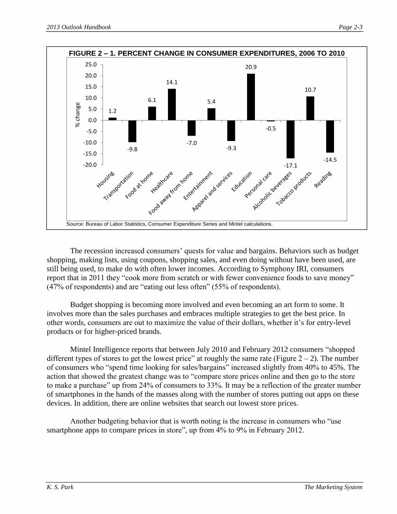
Consumers have increased their expenditures for housing, insurance, and healthcare, and adjusted by
decreased spending in more discretionary items, such as food away from home, apparel and services, and
personal care. Shifts in some expenditure categories are likely meant to decrease overall spending, such as the
increase in food at home spending to offset the decrease in food away from home spending (Figure 2 – 1).
Education expenditures increased significantly. In part this may be due to large increases in college tuition. In
addition, it might also be due to delayed entry into the work force. As students graduate from college and are
unable to find jobs, some may choose to delay their entry into the work force and attend graduate school. This
tactic has been used by students in other recessionary periods.
2013 Outlook Handbook Page 2-3
K. S. Park The Marketing System
The recession increased consumers’ quests for value and bargains. Behaviors such as budget
shopping, making lists, using coupons, shopping sales, and even doing without have been used, are
still being used, to make do with often lower incomes. According to Symphony IRI, consumers
report that in 2011 they “cook more from scratch or with fewer convenience foods to save money”
(47% of respondents) and are “eating out less often” (55% of respondents).
Budget shopping is becoming more involved and even becoming an art form to some. It
involves more than the sales purchases and embraces multiple strategies to get the best price. In
other words, consumers are out to maximize the value of their dollars, whether it’s for entry-level
products or for higher-priced brands.
Mintel Intelligence reports that between July 2010 and February 2012 consumers “shopped
different types of stores to get the lowest price” at roughly the same rate (Figure 2 – 2). The number
of consumers who “spend time looking for sales/bargains” increased slightly from 40% to 45%. The
action that showed the greatest change was to “compare store prices online and then go to the store
to make a purchase” up from 24% of consumers to 33%. It may be a reflection of the greater number
of smartphones in the hands of the masses along with the number of stores putting out apps on these
devices. In addition, there are online websites that search out lowest store prices.
Another budgeting behavior that is worth noting is the increase in consumers who “use
smartphone apps to compare prices in store”, up from 4% to 9% in February 2012.
FIGURE 2 – 1. PERCENT CHANGE IN CONSUMER EXPENDITURES, 2006 TO 2010
Source: Bureau of Labor Statistics, Consumer Expenditure Series and Mintel calculations.
1.2
-9.8
6.1
14.1
-7.0
5.4
-9.3
20.9
-0.5
-17.1
10.7
-14.5 -20.0
-15.0
-10.0
-5.0
0.0
5.0
10.0
15.0
20.0
25.0
% c
han
ge

Page 2-4 2013 Outlook Handbook
The Marketing System K. S. Park
Coupons: For years, shoppers have saved money on name brands by clipping coupons. The number
of coupons redeemed by consumers peaked in the late 1980s and early 1990s, but redemptions steadily
declined since then until 2009, the year after the recession hit. For the last 3 years, redemptions increased
(Figure 2 – 3). Manufacturers used coupons to boost interest and sales and attract customers to new products,
while consumers increasingly used coupons to save money on the brands they wanted to buy. However, in
early 2012 some brands offered fewer and less attractive face values and less time available to use the
coupons, thereby, decreasing the number of redemptions.
FIGURE 2 – 2. SHOPPING BUDGETING BEHAVIOR,
FOOD AND HOUSEHOLD ITEMS JULY 2010 vs. FEBRUARY 2012
Source: The Budget Shopper-US-June 2012, Mintel
9
18
25
33
45
51
4
16
21
24
40
52
0 20 40 60
I use smartphone apps to compare prices in store
I have gone back to a store to get a discount on aproduct because it went on sale after I bought it
I spend a lot of time thinking about things I'd liketo have
I compare store prices online and then go to thestore to make a purchase
I spend a lot of time looking for sales/bargains
I shop at different types of stores to get thelowest price on the item I want
% of respondents
"When it comes to purchasing food and other household items have you done/do any of the following?"
Jul 2010 Feb 2011

2013 Outlook Handbook Page 2-5
K. S. Park The Marketing System
What may boost interest in coupons are the availability now of coupons on the web. E-coupons can
be found on manufacturers’ sites, retailers’ sites, coupon aggregation sites, and e-deals sites (Figure 2 – 4).
Manufacturers’ and retailers’ sites are the most popular, used by more than one-third of shoppers.
Interestingly, one-third of shoppers download coupons from couponing sites. Even new, budget-saving
business concepts, such as Groupon, are accessed by almost a quarter of shoppers.
What will be interesting will be to observe the interactions between the use of traditional coupons,
digital coupons, and the other cents-off shopping behaviors used by consumers, such as mobile coupons,
online price comparisons, and smartphone price comparison apps. Already, Symphony IRI reports that
wealthier shoppers use e-planning tools more than lower-income shoppers. In addition, they recommend that
businesses need to market to consumers at home where many of the shopping decisions are being made rather
than in the store.
FIGURE 2 – 3. COUPON DISTRIBUTION AND REDEMPTION
Source: NCH Coupon Facts Report, NCH Marketing.
0
0.5
1
1.5
2
2.5
3
3.5
4
4.5
5
0
50
100
150
200
250
300
350
2000 2002 2004 2006 2008 2010
bill
ion
s re
dee
med
bill
ion
s d
istr
ibu
tio
n
Couponsdistributed
Couponsredeemed

Page 2-6 2013 Outlook Handbook
The Marketing System K. S. Park
Manufacturing and Retail Trends
Food and beverage and other consumer packaged goods manufacturers introduced at total of 31,649
new food and nonfood products in 2011. New food items totaled 16,212 and nonfood totaled 15,437. This
was the smallest number of introductions in a single year since a high of 47,770 in 2010 (Figure 2 – 5). Prior
to 2008 new food introductions were greater than nonfood, however, after the recession nonfood items
continued their growth until 2011. The decline in food introductions was the first year-over-year decline since
2002. Tightened credit and inventory reduction management on the part of retailers have influenced
manufacturers to reduce their new product introductions. In addition, retailers have managed their store
assortments more tightly, often eliminating unprofitable product lines and trying to simplify the shopping
experience.
FIGURE 2 – 4. DIGITAL MEDIA USAGE
Source: CPG 2011 Year in Review, Symphony IRI.
37
36
33
22
0 10 20 30 40
Download coupons from manufacturer websites
Download coupons from retailer websites
Download coupons from coupons sites, such asSmartSource
Visit online deal sites, such as Woot.com andGroupon
% of respondents

2013 Outlook Handbook Page 2-7
K. S. Park The Marketing System
Supermarket formats continue to lose share to supercenters and warehouse clubs (Figure 2 – 6). In
2000, supermarkets earned almost 70% of consumers’ food expenditures whereas in 2011 they earned only
63.8%. Supercenters and warehouse clubs in the meanwhile had a 7.2% share in 2000 and 16% in 2011. One
of the newest competitors in retail food is AmazonFresh. AmazonFresh is a subsidiary of the retail
powerhouse Amazon. It is test marketing online ordering and home delivery of groceries in the Seattle area.
Online ordering and home delivery is offered by a few retailers, most notably Peapod as a part of Ahold USA,
and FreshDirect in the New York City metropolitan area, although, historically, the model has logistical
challenges that have limited entry by other retailers.
Consumers’ interest in local foods and direct marketing continues to grow. However, direct farm
sales, captured under the category farmers, processors, wholesalers, and other, have not contributed enough
sales to capture share from the other retail expenditure categories. Percent sales from farmers, processors,
wholesalers, and other where 6.0% in 2000 and have remained relatively steady since.
FIGURE 2 – 5. NUMBER OF NEW PRODUCT INTRODUCTIONS OF CONSUMER PACKAGED GOODS
Source: Datamonitor
-
5,000
10,000
15,000
20,000
25,000
30,000
1992 1995 1998 2001 2004 2007 2010
# o
f n
ew p
rod
uct
s
Food and beverage
Nonfood

Page 2-8 2013 Outlook Handbook
The Marketing System K. S. Park
The U.S. Food Marketing System Update
GDP lifted manufacturers’ moods early in 2012 although the effects of Sandy in the heavily
populated East Coast has caused some uncertainties in already softening sales. Unemployment continues to
drop but at a slower-than-hoped-for pace. Although these 2 economic measures improved over 2011, the
forecasts for 2013 GDP and unemployment do not look as hopeful, as inflation forecasts for 2013 could cause
slower economic activity. Consumer price inflation is forecast to increase slightly, to 2.5%, in 2013 and
inflation for food at home is expected to increase even more and is forecast for 3.5% inflation (Table 2 – 1).
TABLE 2 – 1. ECONOMIC SNAPSHOT
Economic Measure 2008 2009 2010 2011 2012
(forecast) 2013
(forecast)
GDP (annual % chg)1 -0.3% -3.1% 2.4% 1.8% 2.1% 1.6%
Unemployment (%, SA)1 5.8% 9.3% 9.6% 9.0% 8.1% 7.8%
Consumer Price Inflation (% chg)
1 3.8% -0.3% 1.6% 3.1% 2.2% 2.5%
Consumer Price Inflation, All Food (% chg)
2 5.4% 1.9% 0.8% 3.7% 3.0% 3.5%
1 Historical data from Bureau of Economic Analysis; forecasts The Conference Board
2 Historical data from Bureau of Labor Statistics; forecasts by USDA-Economic Research Service
FIGURE 2 – 6. SALES OF FOOD AT HOME BY TYPE OF OUTLET
Source: USDA-ERS, Food Expenditures Dataset, table 14. http://www.ers.usda.gov/data-products/food-expenditures.aspx.
0%
10%
20%
30%
40%
50%
60%
70%
80%
90%
100%
2000 2002 2004 2006 2008 2010
% o
f fo
od
exp
end
itu
res
Farmers, processors,wholesalers, and other
Home deliveries, mailorders
Other stores
Mass merchandisers
Warehouse clubs andsupercenters
Specialty food stores
Other grocery
Convenience stores
Supermarkets

2013 Outlook Handbook Page 2-9
K. S. Park The Marketing System
Business thus faced with protracted weak demand has even weaker sentiment and has been slow to invest in capital and human capital. Uncertainty over tax rules and the fate of the fiscal cliff, along with continued austerity at the state and local level, further slow the overall pace of demand. Finally, slow growth abroad limits trade prospects. These conditions are likely to keep economic growth below 1.5 percent (annualized) through mid-2013.
CEOs’ assessment of current conditions remains weak and they have grown increasingly pessimistic
about the short-term outlook. Sluggish growth and a persistent cloud of uncertainty have played a role in
CEOs curtailing spending plans this year.”
Consumer Confidence Index at Highest Level Since February 2008
Food retailers and manufacturers responded to economic downturn. They delayed price increases
during increasing commodity prices, dropped prices on selected core staples in response to consumer bargain
shopping, increased their focus on private labels, increased face value on coupons, and used aggressive price
promotions (sales) to keep prices down and maintain, or even improve, volume. Retail competition was
driven by price in the fear that bargain-hunting shoppers, lacking any store loyalty, would turn to competitors.
Consumer Food Expenditures
The USDA-Economic Research Service estimates for 2011 food and beverage sales from retail
outlets are in Table 2-3 below. A high consumer price index for food in 2011 contributed greatly to the sales
increases. Sales for total food and beverages amounted to almost $1.5 trillion, a growth of 5.5% above 2010
sales. Although the growth in food away from home sales was not shabby, the growth in food at home sales
substantially outpaced it at 4.8% versus 6.0% growth respectively. The reason for much of this difference can
be attributed to the very low inflation rate (1.9%) for food away from home, as restaurants and other eating
establishments held most prices steady in 2011.
TABLE 2 – 2. ECONOMIC INDICATORS
Economic Indicator November 2012
(change from previous month)
Consumer Confidence 0.6points
CEO Confidence -5.0 points
Employment Trends Index 0.53%
Leading Economic Index 0.2%
Source: The Conference Board, http://www.conference-board.org/ accessed November 27, 2012
TABLE 2 – 3. FOOD SALES1
Sector 2011 2010 Growth
--$ million-- %
Total food and beverage sales $1,480,692 $1,403,476 5.5%
Total food sales (excluding alcohol) 1,317,828 1,250733 5.4%
Food at home sales 654,422 617,475 6.0%
Food away from home sales 588,926 561,792 4.8%
Alcoholic beverage sales 162,864 152,743 6.6% 1 Sales only. Does not include home production, donation, or school lunch program expenditures
Source: USDA-ERS, http://www.ers.usda.gov/Briefing/CPIFoodAndExpenditures/Data/Expenditures_tables/table1.htm.

Page 2-10 2013 Outlook Handbook
The Marketing System K. S. Park
The Consumer Price Index
While the drought in the summer of 2012 caused much uncertainty in the food industry, the effects
were somewhat spotty, affecting the grain commodities most heavily. It appears that the effects will not affect
food prices unduly. They are having a delayed effect on meat prices and the effects on CPI for food will not
be seen until 2013 and those will effect meats primarily.
Food inflation has been decreasing the latter part of 2012, such that the changes in the October 2012
CPI for all foods from year ago levels was only 1.7% (Table 2 – 4). The U.S. Department of Agriculture
predicts inflation for all foods to be in the range of 3.0 – 4.0% above 2012 prices. Dairy and fresh vegetable
prices are predicted to see higher than average inflation in 2013. Fish and seafood, fats and oils, processed
fruits and vegetables, and sugar and sweets prices are predicted to see lower than average inflation.
The lack of consumer confidence in the economy along with continued high unemployment levels are
making it difficult for eating establishments to increase prices. The CPI for food away from home is forecast
to increase 2.5 – 3.5% for 2013. Although this is better than 2010 and 2011 levels, it is less than pre-recession
levels.
TABLE 2 – 4. CHANGES IN FOOD PRICE INDEXES, 2010 THROUGH OCTOBER 2011
2010 2011 Oct.
20121
2013 Forecast
% change from year ago
All food 0.8 3.7 1.7 3.0-4.0
Food away from home 1.3 1.9 2.7 2.5-3.5
Food at home 0.3 4.8 1.0 3.0-4.0
Meats, poultry, and fish 1.9 7.4 2.4 3.0-4.0
Meats 2.8 8.8 1.7 3.0-4.0
Beef and Veal 2.9 10.2 5.5 3.0-4.0
Pork 4.7 8.5 -2.1 3.0-4.0
Poultry -0.1 2.9 5.5 3.0-4.0
Fish and seafood 1.1 7.1 1.4 2.5-3.5
Eggs 1.5 9.2 0.1 3.0-4.0
Dairy products 1.1 6.8 -1.1 3.5-4.5
Fats and oils -0.3 9.3 3.0 2.0-3.0
Fruits and vegetables 0.2 4.1 -0.1 3.0-4.0
Fresh fruits & vegetables 0.7 4.5 -0.4 3.5-4.5
Fresh fruits -0.6 3.3 2.1 3.0-4.0
Fresh vegetables 2.0 5.6 -3.2 4.0-5.0
Processed fruits & vegetables -1.3 2.9 1.1 2.0-3.0
Sugar and sweets 2.2 3.3 0.6 2.0-3.0
Cereals and bakery products -0.8 3.9 0.9 3.0-4.0
Nonalcoholic beverages -0.9 3.2 -0.4 2.0-3.5 1 change from year ago October prices. Bureau of Labor Statistics, Inflation and Prices,
http://www.bls.gov/data/#prices.
Source: USDA-ERS, Food CPI, Prices, and Expenditures, http://www.ers.usda.gov/data-products/food-price-outlook.aspx

2013 Outlook Handbook Page 2-11
K. S. Park The Marketing System
Despite the economy, food expenditures as a percent of disposable income remain low. In 2000,
families and individuals spent 9.9% of their disposable income on food. The share disposable person income
has increased slightly the last three years, and inflationary increases in food expenditures concurrent with
stagnating incomes continue (Figure 2 – 7).
The marketing system in the United States is responsible for all the costs incurred in getting food
from the farmers’ gate into the hands of the consumer. It divides the system into ten industry groups: farm and
agribusiness, food processing, packaging, transportation services, energy, retail trade, foodservices, finance
and insurance, advertising, and legal-accounting-bookkeeping services. As the U.S. consumer has demanded
food in more convenient forms, these costs have increased at a faster rate than farmers’ costs and profits.
USDA calculates marketing costs for food produced and consumed in the United States.
A new and expanded food dollar series from USDA-Economic Research Service replaces the
old food dollar series. It provides an overview of the food system, with more accurate estimates of
the farm share and of the distribution of food-dollar value added shares over time. Highlights from
the series include:
For every dollar spent in 2010 in the U.S. on domestically produced food (food dollar), U.S. farmers
sold 14.1 cents of farm products to non-farm establishments (farm share). After spiking in 2007-08,
the farm share of food dollar expenditures in 2010 has returned to the 2006 level.
FIGURE 2 – 7. FOOD EXPENDITURES AS A SHARE OF DISPOSABLE PERSONAL INCOME
Source: USDA-ERS, Food CPI, Prices and Expenditures. http://www.ers.usda.gov/Briefing/CPIFoodAndExpenditures/Data/Expenditures_tables/table7.htm .
5.9 5.9 5.9 5.8 5.7 5.8 5.6 5.6 5.5 5.6 5.6 5.7
4.0 3.9 3.8 4.0 3.9 4.1 4.1 4.1 4.0 4.1 4.1 4.1
0.0
2.0
4.0
6.0
8.0
10.0
12.0
2000 2002 2004 2006 2008 2010
% o
f d
isp
osa
ble
inco
me
Food away from Home
Food at Home
9.9 9.9 9.8 9.9 9.7 9.9 9.7 9.7 9.5 9.7 9.7 9.8

Page 2-12 2013 Outlook Handbook
The Marketing System K. S. Park
Foodservice costs contribute by far the greatest share of expenditures. In 2010 foodservice share was
29.4 cents. However the share of foodservice has been declining since 2004, well before the recession
in 2008.
Food processing costs per food dollar have increased 17 percent since 2008 and are now 21.7 cents of
the 2010 food dollar.
The share of food retailers' costs for food-at-home expenditures has declined 7 percent since 2006 to
23.1 cents in 2010.
Energy costs per food dollar declined nearly 30 percent since 2008 and are now 4.8 cents of the 2010
food dollar.
FIGURE 2 – 8. SHARES OF CONSUMER FOOD EXPENDITURES, BY INDUSTRY GROUP
Source: USDA-ERS. Food Dollar Series. http://www.ers.usda.gov/data-products/food-dollar-series.aspx
0
5
10
15
20
25
30
35
40
2000 2001 2002 2003 2004 2005 2006 2007 2008 2009 2010
Foodservices
Food processing
Retail trade
Farm & Agriculture
Finance & Insurance
Energy
Packaging
Transportation
Advertising
Legal & Accounting

R.M. Severson and T.M. Schmit Cooperatives
Chapter 3. Cooperatives
Roberta M. Severson, Extension Associate, and Todd M. Schmit, Associate Professor
Farmer cooperative sales throughout the United States and New York State set new records in 2011,
which demonstrates the vitality of the nation’s farmer-owned cooperatives and the important role they play in
the agricultural sector. Total net business volume of cooperative businesses (excludes sales between
cooperatives) grew by 24 percent nationally and 22 percent in New York State. Noteworthy research has
been conducted over the past several decades to document the importance of cooperative businesses. Similar
to investor-owned firms, cooperatives must adapt to a variety of external and financial factors in order to
remain profitable and add value to the businesses of their producer members. The following chapter provides
an overview of cooperative activity within the United States and New York State and provides insight into the
critical issues facing cooperatives in the future.
U.S. Situation – Farmer Cooperatives
In 2011, 2,285 U.S. farmer cooperatives owned by 2.3 million members had a record-breaking year
with over $213 billion in gross business volume (includes sales between cooperatives) and nearly $613
million returned to member owners in patronage refunds (Table 3-1). Higher commodity prices in 2011
resulted in farmer cooperatives nationwide (excluding the Farm Credit System) increasing gross business
volume by 11 percent from the previous record high of $191.9 billion set in 2008. This is also a $41.3 billion
increase, or 25 percent over 2010. Table 3-1 compares volume of cooperative business between 2010 and
2011.
TABLE 3-1. U.S. FARMER COOPERATIVES, COMPARISON OF 2010 AND 2011
Item
Gross Business Volume
Marketing Farm Supplies Services Total
Balance sheet
Assets Liabilities Equity Income Statement
Sales (Gross) Patronage income Net income before taxes Employees
Full-time Part-time, seasonal Total
Membership
Cooperatives
2010
($ billion) $101.1 63.9 5.0 $170.1
$65.0 39.0 26.0
$171.8 0.7 4.3
(Thousand) 129.0 54.4 183.4
(Million) 2.2
(Number) 2,314
2011
($ billion) $128.1 80.9 4.5 $213.4
$78.5 50.6 27.9 $213.4 0.6 5.4 (Thousand) 130.9 52.8 183.7
(Million) 2.3
(Number) 2,285
Change
percent
26.7% 26.8
-10.0 25.4%
20.8% 29.7
7.3
24.3% -11.4 25.6
1.5% -2.8
0.2%
4.5%
-1.3%
Source: Cooperative Statistics 2011, USDA Office of Rural Development http://www.rurdev.usda.gov/BCP_Coop_DirectoryAndData.html

Page 3-2 2013 Outlook Handbook
Cooperatives R.M. Severson and T.M. Schmit
While not shown, net business volume (excludes sales between cooperatives) grew by 24 percent or
$35.8 billion from $147.8 billion in 2010 to $183.6 billion in 2011. Most of this (82%) can be attributed to
increasing dairy and grain and oilseed prices, with dairy product marketing cooperative volume increasing by
$8 billion and grain and oilseeds marketing cooperative volume increasing by $13.4 billion. Net business
volume for supply cooperatives increased $10.2 billion, with increasing prices paid for feed, fertilizer, and
petroleum accounting for 87% of the increase. Net business volume increased $1.9 billion, $2.3 billion, and
$3.6 billion for feed, fertilizer, and petroleum products, respectively.
The aggregate cooperative balance sheet shows total assets increased by $13.5 billion or 21 percent
and liabilities increased by $11.6 billion or 30 percent between 2010 and 2011. Equity improved by $1.9
billion or slightly over 7%. Net income before taxes increased $1.1 billion or 25.6 percent between 2010 and
2011.
Nationally, farmer marketing cooperatives account for 53.5 percent of all farmer cooperatives with
36.6 percent of all memberships. Supply cooperatives account for 40.9 percent of all U.S. farmer
cooperatives and 61.7 percent of all memberships. Farmer service cooperatives make up the balance; i.e. 5.6
percent of cooperatives with 1.7 percent of memberships. Membership numbers exceed farm numbers as a
farm business can belong to one or more cooperative enterprises. The total number of cooperatives declined
modestly between 2010 and 2011 (-1.3 percent), reflective of continued industry consolidation (Table 3-1).
While farmer cooperative members have also trended downward over the last decade, total memberships
increased modestly between 2010 and 2011 by 4.5 percent. This result was largely influenced by strong
growth in the number of grain and oilseed cooperative memberships (+159,000) that more than offset
relatively sizable declines in memberships for tobacco marketing cooperatives (-53,000) and supply
cooperatives in total (-64,100).
The number of full- and part-time workers remained relatively constant in 2011 at 183.7 thousand
workers, with a modest increase (1.5 percent) in full-time workers to 130.9 thousand (Table 3-1). Notably,
full-time employment is up over 7 percent from its five-year low in 2009. Marketing cooperatives employ 57
percent of the farmer cooperative labor force, followed by supply cooperatives at 42 percent, and service
cooperatives at 1 percent. Grain and oilseed marketing cooperatives employed 24,300 employees, with an
increase of 8 percent from 2010 to 2011. Likewise, dairy cooperatives employed 20,800 employees in 2011,
with an increase of 10 percent over 2010. Fruit and vegetable marketing cooperatives employed 13,500
employees in 2011, with an increase of 1.5 percent over 2010. These three sectors employ approximately 45
percent of all farmer cooperative workers.
New York State Situation
Data for agricultural cooperatives headquartered in New York State were obtained through a USDA
Rural Development Cooperative Service survey. The most current state-level information available is for
years 2010 and 2011. Table 3-2 summarizes cooperative businesses headquartered in New York State.
Between 2010 and 2011 the total number of farmer cooperatives (55) and cooperative memberships
(6.4 thousand) were stable. The number of dairy cooperatives and the number of fruit and vegetable
cooperatives decreased by one in each category, while the number of “other product” marketing cooperatives
increased by two. Dairy and fruit and vegetable cooperatives maintained membership as cooperatives are
more likely to merge rather than disband. Two “other products” marketing cooperatives reported to the
survey increasing membership by 100.
Reflective of improved milk prices in 2011, net business volume for dairy cooperatives increased by
nearly $405 million or 23 percent from 2010 levels. New York State dairy cooperatives market
approximately 75 percent of the milk produced within the state. Fruit and vegetable and other products

2013 Outlook Handbook Page 3-3
R.M. Severson and T.M. Schmit Cooperatives
TABLE 3-2. NEW YORK STATE AGRICULTURAL COOPERATIVE NUMBERS, MEMBERSHIPS AND NET BUSINESS VOLUME, 2010 and 20111
Major Business Activity
Number & Membership (000) Headquartered in State
Net Business Volume
2010 2011 2010 2011
No.
Members (000)
No.
Members (000)
($ million)
Marketing: Dairy Fruit & Vegetable Other Products
2
TOTAL MARKETING
Supply: Crop Protectants Feed Fertilizer Petroleum Seed Other Supplies
TOTAL SUPPLY
TOTAL SERVICE3
TOTAL
31 3.5 30 3.5 9 1.0 8 1.0 3 0.2 5 0.3
43 4.7 43 4.8
6 1.4 6 1.4
6 0.3 6 0.2
55 6.4 55 6.4
$1,738.5 $2,143.4 70.5 74.8 170.8 184.8
$1,979.7 $2,403.0
$13.2 $22.9 71.6 74.3 18.1 31.4 2.5 2.3 2.7 3.6 19.5 27.5
$127.7 $162.0
$15.5 $31.5
$2,123.0 $2,596.6 Source: Cooperative Statistics 2011, USDA Rural Development, http://www.rurdev.usda.gov/BCP_Coop_DirectoryAndData.html
1 Totals may not add due to rounding.
2 Includes wool, poultry, dry bean, grains, livestock, maple syrup, ethanol, and miscellaneous cooperatives.
3 Includes those cooperatives that provide services related to cooperative marketing and purchasing.
cooperatives increased volumes by 6 percent and 8 percent, respectively, and resulted in net business volume
for all reporting marketing cooperatives to increase by $423.3 million or 21 percent.
The database indicates that there are six farmer supply cooperatives and six farmer service
cooperatives in New York State. Producers experienced higher costs for inputs in 2011 and these higher costs
are reflected in higher business volumes for crop and livestock inputs in supply cooperatives. Net business
volume from seed sales increased 30 percent and net business volumes from crop protectants and fertilizer
increased by over 70 percent each. In total, net business volume for supply cooperatives increased by $34.4
million, or 26.9 percent. The robust increase in farmer cooperative services resulted in net business volume
doubling from $15.5 million to $31.5 million. Overall, net business volume for those cooperatives
headquartered in New York State increased by $473.6 million or 22 percent.
The USDA Rural Development Cooperative Survey does not include activity of the Farm Credit
System. According to the 2011 Farm Credit East Annual Report, on January 1, 2010 Farm Credit of Western
New York, ACA merged into First Pioneer Farm Credit, ACA to create Farm Credit East, ACA. Farm Credit
East, ACA service area includes New York State, New Jersey, Massachusetts, Connecticut, Rhode Island,
New Hampshire, and customers in several other states. As such there are no figures specific to New York
State; however 52 percent of the loan portfolio is based in New York State. The 2011 Farm Credit East ACA
annual report notes that loan volume increased slightly less than 2 percent from $4.3 billion to $4.4 billion.
Net income before taxes rose from $134.43 million to $141.40 million. The board of directors determined
that $35.5 million be returned in cash refunds, the cooperative’s 16th consecutive patronage distribution.

Page 3-4 2013 Outlook Handbook
Cooperatives R.M. Severson and T.M. Schmit
Issues for Agricultural Cooperatives
In 2011, the Council on Food, Agriculture, and Resource Economics (C-FARE) convened a panel of
24 cooperative CEOs, USDA researchers, and academic specialists to learn more about critical issues facing
today’s cooperatives. Cooperative businesses are different from other types of investor owned firms in that
they are owned by member patrons who have democratic control with a portion of the net revenues returned
to members through patronage refunds. Panelists were asked to rate a series of issues as extremely important,
very important, important, somewhat important, and not important. The issues were grouped as shown in
Figure 3-1.:
FIGURE 3-1. CRITICAL ISSUES FACING COOPERATIVES, C-FARE PANEL, 2011
Issue Sub-issues
External
Industrial competition
Market concentration
Public policy
Regulation
Global competition
Consumer preferences
Market volatility
Finance
Tax issues
Outside equity
Unallocated equity
Risk management
Profitability
Financial competency
Adequate equity
Strategy
Decision making
Aligning incentives
Cooperation with cooperatives
Efficiency
Succession
Human resources
Planning
Governance
Balancing cooperative and member needs
Board dedication
Board competency
Member involvement
Board operations
Board orientation
Recruiting board members
Communication Public understanding
Educating youth
Educating members
Value to members
Source: Kenkel and Park, 2011.
The following is a brief summary of the panel results.
EXTERNAL: Market volatility and public policy were deemed extremely important to very
important by 80 percent of participants. Over 60 percent identified industry competition, market
concentration and global competition as extremely important or very important. Nearly one-third of the panel
viewed consumer preferences as extremely important.
FINANCE: Financial issues are one way to examine factors internal to the cooperative business.
Profitability was rated extremely to very important by all respondents. In addition, 90 percent of respondents
indicated that adequate equity and financial competency was extremely important or very important. The
cooperative profit stream is used to build equity for the cooperative businesses while simultaneously returning
patronage and retiring equity of member owners. The most critical challenge identified was the need to
acquire and maintain equity accounts that would finance growth and provide working capital when necessary.
The second financial challenge identified was the need for adequate profitability to finance the assets and
strengthen the balance sheet. Most equity capital is derived from earnings. The third most mentioned
challenge was balancing the tradeoff of the proportion of equity investment on the part of the member with
the need of the cooperative to retain more equity as a risk management tool.

2013 Outlook Handbook Page 3-5
R.M. Severson and T.M. Schmit Cooperatives
STRATEGY: External and financial issues can be addressed and managed through competent people
with the ability to create and implement a strategic plan that positions the cooperative for growth and returns
to members and patrons. Almost 90 percent of the panel indicated that a sound strategic plan was important
to extremely important. Over 90 percent of the panel indicated that human resources were critical to the
success of the cooperative enterprise. More specifically, “…[T]he succession of management and key
personnel, attracting and maintaining high quality personnel, and aligning the incentives of managers and
employees with member interests all received high importance ratings.” (Kenkel and Park, 2011).
GOVERNANCE AND COMMUNICATION: Competent employees and management is critical to
the success of a cooperative business. At the same time there is a need for competent cooperative board.
Eighty percent of the panelists suggested that recruiting board members with the necessary critical thinking
skills and decision making capabilities is extremely important, with the remaining 20 percent indicating that
this is very important. Board members are the linkage representing the interests of the members when making
decisions regarding cooperative policies and goals. The directors are charged with rationalizing business
decisions to members that ultimately impact equity funds retained in the cooperative business and profits
distributed patrons. Over 60 percent of the panel indicated that communicating the value of the cooperative
business to its members was extremely important, with another 30 percent indicating that it was very
important.
Cooperative Outlook for New York
Through a resolution passed by the United Nations, 2012 was designated the International Year of the
Cooperative. The International Cooperative Alliance found that the combined economic activity of the top
300 cooperatives in the world would create the 9th largest economy (World Cooperative Monitor). Nine of the
top fifty-one dairy cooperatives within the United States have members in New York State and of those nine,
five are headquartered in New York State (Hoard Dairyman 2012). Cooperatives play a significant role in the
farm and food sector in the state.
The initial high temperatures and subsequent freezing temperatures experienced by fruit growers in
early spring decreased fruit yields significantly. Decreased fruit yields will likely impact the financial
statements of fruit cooperatives over the next two years. Drought conditions of 2012 have reduced the
roughage available to dairy farms. Some farmers were able to harvest additional cuttings and others double
cropped small grain acreage as a means to close the gap of forage demands of dairy cattle. Drought
experienced throughout the Midwestern part of the United States increased price levels and volatility in grain
markets. As a result, one of the biggest challenges facing dairy farmers is the volatility in grain markets and
subsequent input costs coupled with a decreasing milk price. Cooperative leaders and farmers have voiced
concerns over the lack of passage of the Farm Bill and the impending “fiscal cliff” with the potential negative
impact on the economy and consumer purchasing patterns.
Dairy cooperatives have voiced concern over expanding milk supply to meet the increasing need for
product for yogurt production. Cooperatives partition the milk produced by member farms to existing and
potential customers. Class I milk sales are preferred because of the higher prices received compared to Class
II, III, or IV. In spite of transportation costs, shipping milk from the Northeastern United States to the Class I
deficit areas of the Southeastern United States can result in higher average milk prices received by dairy
farmers, even though there is increased local demand for Class II milk for yogurt production. The reality is
that dairy cooperatives do not increase the supply of milk in the market. Growth decisions are made by
individual farm businesses. “Each owner makes this decision on the basis of their business, and often the
family’s goals and the opportunities that they see before them. Growth may be an industry goal, but it is a
firm decision.” (Novakovic, 2012).
Profitability is key for any business to remain viable into the future. Profitability within a business is
influenced by internal controls responding to external conditions. Cooperatives have and will continue to

Page 3-6 2013 Outlook Handbook
Cooperatives R.M. Severson and T.M. Schmit
investigate opportunities to build joint ventures that leverage resources, minimize risk, and build profitability.
Unique to the cooperative business model is to return patronage income to their members and, as such, the
cooperative becomes an extension of and adds value to the members business. Several boards of directors
and management are actively engaging in the strategic planning process to chart a course of action that
embraces both the challenges and opportunities for the cooperative business to align with the goals of the
membership.
Although 2012 brought a number of trials to cooperatives and their farmer members operating in New
York State, these farmer-owned businesses will remain well positioned for solid performance in 2013.
References
Farm Credit East, ACA. The Power of Collaboration, Farm Credit East Annual Report 2011.
Johnson, Chelsey, “Top 50 Cooperatives Boost Production Despite Having Fewer Member Farms,” Hoards
Dairyman, October 11, 2012, 157(17): p.643.
Kenkel, Phil and John Park, “Theme Overview: Critical Issues For Agricultural Cooperatives,” Choices, The
Magazine of Food, Farm and Resource Issues, 3rd
Quarter 2011, 26(3).
Novakovic, Andrew M., “The Chobani Paradox,” Program on Dairy Markets and Policy Briefing Paper
Series, March 2012, accessed November 24, 2012 at http://dairy.wisc.edu/pubPod/pubs/BP12-03.pdf.
The World Cooperative Monitor, Exploring the Cooperative Economy, http://issuu.com/euricse/docs/wcm
2012_issue/23#print
USDA. Annual Farmer, Rancher, and Fishery Cooperative Statistics, 2011, Office of Rural Development
accessed November 1, 2012 at http://www.rurdev.usda.gov/BCP_Coop_DirectoryAndData.html.

C.G. Turvey Finance
Chapter 4. Finance Calum G. Turvey, Professor
General Outlook
It is difficult to gage precisely what the financial status is in New York because the USDA no longer
includes NY in its agricultural resource management surveys. However some indication of the financial state
can be gleaned from the Financial Report of Farm Credit East through September 30 2012. According to the
report dairy loans make up 23.1% of the portfolio, cash crops 11.2% and other livestock 9.6%. Farm Credit
East reports continued stress in timber, tobacco, green house, nursery and sod but there is no indication of
wide-spread credit deterioration of the major dairy, cash crops or livestock sectors.
Nonetheless nonaccrual loans increased from 48,722 million in 2011 to 84,879 million through 2012,
an increase of 74%. Including 90-day past due and those being restructured the increase over 2010 has been
65.5%. Total high risk assets increased from $56,418 to $93,396, or by 65.5%, and this has caused Farm
Credit East to increase allowances for loan loss provisions. While overall delinquencies are low at 0.8%, this
has doubled since the same period in 2011.
The supply of credit is ample. According to the Farm Credit System Annual Report (2011), USDA’s
estimate of debt by lender shows that commercial banks held 44 percent of total farm business debt at the end
of 2010. The System’s market share rose to 41 percent from a 40 percent share a year earlier. Kansas Federal
Reserve Agricultural Finance Databook notes that as the costs of production soared throughout 2012 so did
the number of operating loans to keep pace. The Farm credit System’s market share of total farm debt has
been rising steadily over the past decade relative to the commercial bank share. Farm debt owed to the USDA
and to life insurance companies has remained stable while debt owed to individuals, merchants, and other
lender types continue to decline. According to the Kansas City Federal Reserve Farm Databook Delinquency
of non-real estate farm loans in 2012 fell to 1,5% the lowest it has been since the peak of the financial crisis of
about 3.3%. Real estate loans delinquencies held steady at about 3% throughout 2012 down from peak
delinquencies of about 3.75% in 2010, which suggest that the worst of the economic adjustments following
the financial crisis of 2008 are over.
It does not appear that there is any credit tightening in agriculture for either operating expenses or
asset purchase. For example the Kansas Federal Reserve Agricultural Finance Databook notes that as the
costs of production soared throughout 2012 so did the number of operating loans to keep pace. Rates are also
at long-term lows. With livestock loans as low as 4%, operating loans at 4.5% and machinery and equipment
loans at about 5% the financial risk is lower now than in 2007 when rates were at about 9%. These are even
lower than the first part of 2012 with rates ranging from 4.8% to 5.8%. It was also noted that commercial
lenders had no shortage of loanable funds to meet this demand so many of the credit-tightening conditions
that has led to previous busts are not currently at play. The Farm Credit Funding Corporation, which issues
bonds on behalf of the Farm Credit System, is highly regarded and bond ratings have kept pace with U.S.
treasuries so it does not appear that the supply of long-term capital for agriculture is currently at risk.
There are of course pending events that can have major impacts which have more to do with how
farmers vote than how they farm. Congress is misbehaving on two fronts and seems to be willing to drive the
economy of the ‘fiscal cliff’ in terms of negotiating a revenue-balanced deficit reduction plan. Meanwhile,
Congress is also holding up passage of the Farm Bill plowing a path towards the ‘farm cliff’. These two
events, as inconceivable it might be that they are not resolved by the time this goes to print, will have a
devastating effect on the agricultural economy. Most important is the immediate flight of capital out of the
United States. Even if US treasuries (and hence Farm Credit Bonds) are not downgraded (which they most

Page 4-2 2013 Outlook Handbook
Finance C.G. Turvey
surely will be) the notion that congress would purposefully drive the economy towards a double dip recession
will cause many global financiers to lose faith in the U.S. dollar and, the 14th amendment notwithstanding, the
will of Government to back its treasuries. The impact on equity markets globally will be severe with equity
losses far in excess of the amounts of revenue (taxes) being asked of congress. Capital losses will result in a
tightening of credit which will impact the supply of operating loans to agriculture, while the risk attached to
farm credit bonds will increase. Credit will become more costly and in reduced supply. It is unlikely that
further quantitative easing of the money supply will be put in place to resolve a problem of congress’s own
making.
On the other side failure to pass a Farm Bill will return policy to permanent law in which age-old
subsidy rates, such as $38 milk, will enrich many farmers while distorting market based production
incentives, opening up U.S. agriculture to trade litigation, while driving up the deficit. Moreover, any targeted
disaster assistance for 2012 will be lost as will be any modernization of publicly supported revenue assurance
or farm programs targeted towards the current realities of today.
Farmland Values
Agricultural land is, for most farmers, the largest asset item with unrealized capital gains being the
largest contributor to equity. Some extraordinary rises in farmland prices in recent year has led to questions
of whether a bubble exists and if so whether a bust is imminent.
Using reports from the Kansas City Federal Reserve land values are still rising in much of the USA
with Illinois, Indiana, Iowa, Missouri and Wisconsin land prices rising 15% higher than June of 2011,
Maryland, North Carolina South Carolina, Virginia and West Virginia by 6%; Louisiana, New Mexico and
Texas by 11%; Michigan, Minnesota, Montana, North and South Dakota and Wisconsin saw dry land values
increase by 21%, irrigated land fall by 5% and ranchland increase by 6%; Colorado Kansas Missouri
Nebraska New Mexico Oklahoma and Wyoming with dry land increases of 27%, irrigated land increases of
28% and ranchland increases of 18%; and Alabama, Arizona, California, Hawaii, Idaho, Nevada, Oregon,
Utah and Washington saw a 26% increase in irrigated land, a 20% increase in rangeland and a modest 2%
increase in dry land.
With this backdrop farmland prices in NY State have been quite modest as illustrated in Figure 4-1
which shows that prices have increased by $200 in each of the past 3 years according to the USDA or about
8% per year. Even so as Figure 4-2 shows the percentage change in farmland prices has been higher in the
past six years has been higher than the 6 years following 2000.

2013 Outlook Handbook Page 4-3
C. G. Turvey Finance
FIGURE 4-1 NEW YORK STATE FARMLAND VALUES 1997-2012
Source: USDA
The largest rise in farmland prices in New York was 16.9% in 2006 and second was 12.4% in 2008.
The recent rise of about 8% pales in comparison to what is being observed throughout the rest of America. It
should be noted, of course that these prices are as reported by the USDA and not the New York Federal
Reserve. The numbers reported by the Kansas City Reserve are consolidated by the various Federal Reserve
Banks across the United States as reported from transactions data and thus come from a different source than
the USDA estimates. Having said this, it does not appear that there is a farmland price bubble in New York,
at least to the extent of what is seen in the mid-western states. The caveat to this is that farmland prices appear
to be increasing almost regardless of what is going on from year to year in the agricultural economy which is
what agricultural economists refer to as the ‘farmland pricing puzzle’. This immunity to economic forces
suggests that drivers other than the real economy are pushing land prices higher. For example dairy and other
livestock producers need additional land in order to increase herd size so the price of land is driven not by
cash crops but by the incremental benefits to farmers in its alternative use. Also, land parcels come up for sale
so infrequently that farmers are willing to pay a substantial premium for the land above its economic value
because it may be decades later before the parcel comes up for sale again. In other cases farmers can increase
the economic efficiency of the whole farm by adding additional land so the economic benefit is not what can
be obtained marginally on the purchased land but also any economic gains in efficiency for the farm as a
whole. In addition, there is evidence that payments from government programs are capitalized into farmland
values but in reality the role of support and emergency programs will do more to set a floor on the value of
land, rather than a key driver of its rise in value.
1997 1998 1999 2000 2001 2002 2003 2004 2005 2006 2007 2008 2009 2010 2011 2012
Series1 1,020 1,040 1,110 1,180 1,250 1,320 1,390 1,460 1,520 1,800 1,900 2,150 2,200 2,400 2,400 2,600
0
500
1,000
1,500
2,000
2,500
3,000
$/A
cre

Page 4-4 2013 Outlook Handbook
Finance C.G. Turvey
FIGURE 4-2 YEAR-OVER-GROWTH RATES IN FARMLAND VALUES,
NEW YORK 1997-2012
Percentage Change in Farmland Prices
Nonetheless, when land is purchased for more than it’s worth there is a reverse equity transfer where
the current generation of buyers transfers its future equity to the last generation (sellers). This will result in
lower returns to equity in the short and long term. These losses in equity can only be recovered if the rate at
which land values grow turns out to be greater than what was implied by the originating land price. It does not
appear, at least in the short run, that land prices will flatten out or decrease any time soon although anything
can happen at any time. However it should be noted that the busts in farmland markets in the past were driven
by many factors including in the 1920s and 1930s a collapse of farm credit supply from commercial lenders
(leading then to the formation of the Farm Credit System). The driver of the 1980’s boom and bust is largely
attributed to optimism in commodity markets, the perception that land was a hedge against inflation, and
imprudent lending practices that were focused more on asset values and capital gains than cash flow. None of
these factors are in play in 2012 so while history may repeat itself the cause will not be repeated. Rather it
appears that what is occurring in land markets, particularly in the mid-west is more of a greater fool theory in
which individuals will continue to buy land at ever increasing prices so long as they believe that there is a
greater fool to pay an even higher price in the future. If so, all there is to do is wait until the pool of fools runs
out!
1998 1999 2000 2001 2002 2003 2004 2005 2006 2007 2008 2009 2010 2011 2012
Series1 0.019 0.065 0.061 0.058 0.054 0.052 0.049 0.040 0.169 0.054 0.124 0.023 0.087 0.000 0.080
0.000
0.020
0.040
0.060
0.080
0.100
0.120
0.140
0.160
0.180
Axi
s Ti
tle

2013 Outlook Handbook Page 4-5
C. G. Turvey Finance
Financial Conditions of U.S. and NY Farms
As indicated earlier New York is no longer surveyed as part of the USDA’s periodic Agricultural
Resource Management Survey but from past experience financial conditions in New York were fairly
consistent with the financial conditions of farmers elsewhere in the USA. Table 4-1 presents data obtained
from the Agricultural Census to provide a picture of what these financial conditions are.
TABLE 4-1 DEBT POSITION OF U.S. FARMERS
A. General Conditions All <35 35-44 45-54 55-64 >64
Number of farms 2,192,774 96,389 223,386 519,097 698,943 654,958
Age Distribution 1.000 0.044 0.102 0.237 0.319 0.299
Number of farms with debt 645,674 49,099 99,457 191,167 197,240 108,711
% within age 0.294 0.509 0.445 0.368 0.282 0.166
% of All 0.294 0.022 0.045 0.087 0.090 0.050
% of All with Debt 1.000 0.076 0.154 0.296 0.305 0.168
Total Assets 930,003 642,072 807,250 940,743 990,795 940,857
Current Assets 110,620 106,361 114,336 122,086 117,163 93,911
Non-Current Assets 819,382 535,711 692,914 818,657 873,632 846,946
Total Liabilities 79,049 120,539 130,371 106,442 78,373 34,450
Current Liabilities 25,248 36,385 39,636 34,431 24,461 12,263
Non-Current Liabilities 53,801 84,153 90,735 72,012 53,912 22,187
Equity 850,953 521,533 676,879 834,301 912,422 906,408
Debt/Asset Ratio D/A 0.085 0.188 0.162 0.113 0.079 0.037
Debt/Equity Ratio D/E 0.093 0.231 0.193 0.128 0.086 0.038
B. Scenario Analyses With Debt
Assets 930,003 642,072 807,250 940,743 990,795 940,857
Total Liabilities 268458.4 236636.9 292820.6 289033.8 277723.9 207553.1
Equity 661,545 405,435 514,429 651,709 713,071 733,304
Debt/Asset Ratio D/A 0.289 0.369 0.363 0.307 0.280 0.221
Debt/Equity Ratio D/E 0.406 0.584 0.569 0.444 0.389 0.283
C. Scenario Analysis No Debt
Assets 930,003 642,072 807,250 940,743 990,795 940,857
Total Liabilities 0 0 0 0 0 0
Equity 930,003 642,072 807,250 940,743 990,795 940,857

Page 4-6 2013 Outlook Handbook
Finance C.G. Turvey
Overall, farm debt in agriculture is low with plenty of equity for investment and expansion. The debt
to asset ratio sector-wide is only 8.5% and the debt to equity ratio is only 9.3%. However these scenarios are
misleading because they include farms with and without debt. Farms with no debt would hold no mortgage
on the land and would typically have paid off any operating loans or other short term credit. It is significant,
economically speaking, that only 29.4% of American farmers have debt. Thus from a financial point of view
the focus should not be on all farms but those that are exposed to financial risks.
In Part B of Table 4-1 the debt is adjusted using a simple pro-ration to glimpse at what this might
mean. On a pro-rated basis the average debt to asset ratio of farms with debt is 28.9% and the debt to equity
ratio is 40.6%. Even at 28.9%, this is not a degree of over-leverage that will bring widespread harm to the
agricultural economy should a down-turn occur.
What is interesting in Table 4-1 is the classification of financial conditions according to age. As
expected, younger farmers hold more debt relative to assets or equities (36.9% and 58.4%) than older farmers
(22.1% and 28.3%). These are depicted in Figures 4-3 and 4-4.
FIGURE 4-3 D/A AND D/E RATIOS FOR ALL FARMS BY AGE GROUP
Average Debt to Asset and Debt to Equity Ratio for all Farmers and by Age Group
1 2 3 4 5 6
D/A 0.085 0.188 0.162 0.113 0.079 0.037
D/E 0.093 0.231 0.193 0.128 0.086 0.038
0.000
0.050
0.100
0.150
0.200
0.250
Rat
io

2013 Outlook Handbook Page 4-7
C. G. Turvey Finance
FIGURE 4-4 D/A AND D/E RATIOS FOR FARMS WITH DEBT BY AGE GROUP
Average Debt to Asset and Debt to Equity Ratio for all Farmers with debt and by Age Group
FIGURE 4-5 FARMER AGE DISTRIBUTION, TOTAL FARMS=2,192,774
Distribution of Age of U.S. Farmers
All <35 35-44 45-54 55-64 >64
D/A 0.289 0.369 0.363 0.307 0.280 0.221
D/E 0.406 0.584 0.569 0.444 0.389 0.283
0.000
0.100
0.200
0.300
0.400
0.500
0.600
0.700R
atio
<35 35-44 45-54 55-64 >64
Age Distribution 0.044 0.102 0.237 0.319 0.299
Number of farms 96,389 223,386 519,097 698,943 654,958
0.000
0.050
0.100
0.150
0.200
0.250
0.300
0.350
0
100,000
200,000
300,000
400,000
500,000
600,000
700,000
800,000
Age
Co
un
t

Page 4-8 2013 Outlook Handbook
Finance C.G. Turvey
Commentary on the Age Distribution of Farmers
A piece of information in Table 4-1 that is often overlooked in any outlook presentation is the age
distribution of farmers. This is depicted in Figure 4-4. What the figure reveals is that the average age of
farmers is getting quite old. Nearly 60% of farmers are 55 years or older while only about 15% are 44 years or
younger. This raises an important question as to who will be farming in 20 or 30 years. It seems quite clear
that here are not enough young farmers to replace retiring farmers. In 10 years’ time as 519,097 farmers
migrate from the 45-54 age group to the 55-64 age group there are only 223,386 farmers currently aged 35-
44 to replace them leaving a void of 295,711 farmers. In 20 years’ time the group currently 55 or older
numbers 1,353,901 but the group replacing them number only 742,483. Of course more and more young
farmers will enter the business but the problem is not the absolute number but the rate at which they are
entering the business. What Figure 4-4 suggests is a basic problem in population dynamics in which the rate
at which people exit farming exceeds the rate at which there are new entrants will ultimately result in a
significant economic adjustment.
What will this require? If buyers are fewer than is required to absorb land put up for sale upon
retirement then land prices must fall, and in fact will fall, until it is low enough to attract new entrants. On the
other hand, existing farmers must purchase that land and expand their own operations which will require
substantial capital investments and access to credit and credit markets. If capital is available then farmers
wishing to expand might compete and bid up land prices. Failing this is an opening for corporate-agriculture-
what has in previous days been called the suitcase farmers – made up of equity investment funds that will
purchase farmland as an investment and redistribute its worth amongst multiple owners in the form of shares
with the land being managed by private farm management companies. Should these shares become tradable
on formal markets their values can rise and fall on speculative forces by traders who may or may not know
anything about commodity markets let alone agriculture? Initially it will be more or less true that the value of
such shares will be valued according to measureable farm conditions, but one can imagine where the weight
of shares so traded, and the number of traders so large, that there will be a tipping point at which it will
become the equities markets and not agricultural conditions that will ultimately determine the value of land.
This is rather critical. Cash flows from agriculture are typically uncorrelated with cash flows in the industrial
sector and this degree of correlation is very attractive to mutual and pension funds for diversification
purposes. Thus the demand for shares on agricultural land will put additional and upward pressure on the
price for farmland.
New York Dairy
2012 has been a year of mixed blessings for New York farmers with much of the state escaping the
full throat of the great drought that browned the Midwest and record high prices for grains and oilseeds. For
many farmers in the crop sector revenues driven by higher prices offset reduced yields. But as so much of
agriculture history tells us the magical web of the cob-cycle ensures that it is a zero sum gain with one sector
of the economy thriving but at the expense of another sector. For livestock and dairy farmers the rise in corn,
soybean and forage prices was dramatic. If there is one law that always stands it is the law of economics and
in 2012 the gavel defining the laws swung many times.

2013 Outlook Handbook Page 4-9
C. G. Turvey Finance
To say the least, the agricultural economy was not ready for a drought of the magnitude seen in the
Midwest. The structure of agriculture has changed dramatically especially since 2007 when ethanol standards
were set and this change has resulted in a new demand with even greater inelasticity than before. Tying the
price of corn to gas, which in turn is driven by global oil markets, means that a structural shift has occurred
removing part of commodity volatility from the food chain (feed and processing) to some combination of
energy markets and food demand. From this point the agricultural cobweb cycle starts with more land being
put into corn production, and fewer in other grains and oilseeds. That lower supply coupled with increasing
global demand results in all-round increase in crop prices that is favorable to crop producers but placing great
stressors on dairy and livestock producers, particularly grain fed cow calf and finishing operations and poultry
in which the key cost driver is corn. The Midwest drought of 2012 did not help matters. While more than 80%
of crop farmers will receive some relief through crop insurance protection for dairy and livestock producers,
beyond futures and options, is limited.
At the beginning of 2012 the Class III futures prices was $17.34/cwt which was 19.2% lower than its
all-time high of $21.46 on August 29th 2011. Corn at the turn of the New Year was $5.95/bu. By the
beginning of February 2012 Class III milk prices had fallen below $16/cwt while corn was rising towards
$6.50 per bushel. On April 11th milk futures fell below $15 while corn prices held steady, but by mid-June
concerns over a drought in the mid-west became more of a worry and on July 3 corn broke $7/bu and milk
futures had once again broken $17 to close at $17.25. About two weeks later on August 19th corn futures
broke the $8 mark. At the time of this writing on November 14th 2012 corn was holding steady around $7.26
and milk, now oscillating between $19 and $20 was at $19.69. For the year corn prices were up 22% while
milk price were up 13.5%. Corn peaked at an all-time high of $8.3125 on August 21 2012 and on September
4 soybeans hit an all-time price of $17.71/bushel. The cost of feed calculated using weights on corn, soybean
and hay prices as calculated for the MILC program started out the year at $11.071/cwt rising by 14.4% to
$12.66/cwt. The Milk to corn (milk/corn) price ratio started out at 2.67 in January 2012 and closed at 2.71 as
of November 14th 2012.
Given these changes in market structure and market volatility the ratio of class III milk future to corn
futures becomes an important indicator of a price-cost or margin squeeze in the dairy sector. The ratio works
in a couple of dimensions but most important as milk prices rise relative to the price of corn margins tend to
increase, as corn prices rise relative to milk the ratio falls. In fact it does not really matter whether milk prices
rise by 13.5% if corn prices – which makes up the bulk of feed costs – rise at a faster rate of 22%.
To investigate whether there is a strong relationship between net income per cow and the milk/corn
price ratio we gathered the records from 35 dairies in New York who had participated in Cornell’s Dairy
Farm Summary Project between 1997 and 2010. We then averaged the costs across all farms and also
identified the highest and lowest incomes for each year. The results of this investigation are shown in Figure
4-6.

Page 4-10 2013 Outlook Handbook
Finance C.G. Turvey
FIGURE 4-6 DAIRY INCOME PER COW AND MILK/CORN RATIO
Dairy Income per Cow and the Milk/Corn Price ratio 1997-2010
It can be seen from Figure 4-6 that there is a strong relationship between the ratio as an indicator of
stress for all three farm types. Using statistical techniques (linear regression) it is found for the average farm
that a 1 unit increase in the price ratio increases income/cow by $248/year, for the low income farms it is
$429.42/cow and for the high valued farm it is $273.22/cow. Most certainly efficiency is a good hedge against
a margin squeeze but when the ratio falls from 3.5 to 2.5 a less efficient farm would see a reduction of
$429.42/cow.
And why is this important? If we examine the price ratio between 2000 and 2007 (Figure 4-7) when
ethanol standards were set and corn markets began to respond the average price ratio were 5.39. But from
2008 to the present that ratio has fallen by 43.8% to an average of 3.03. By these calculations the net income
per cow between 2000-2007 and 2008-2012 would have fallen by $585.28/cow. For the less efficient farms
the reduction is on average $1,103/cow. On August 10th 2012 the price ratio hit an all-time low of 2.109 when
corn closed at $8.20 and Class III milk closed at $17.3. So in 2012 with the ratio averaging 2.52 farm income
per cow might be $1,232 lower than the 2000-2007 periods for the low efficiency farms and $711.76/cow for
the average farm.
1997 1998 1999 2000 2001 2002 2003 2004 2005 2006 2007 2008 2009 2010
Average 313 933 851 541 865 395 368 953 965 379 1561 938 -199 731
Min -324 149 -64 -159 -92 -437 -501 121 -82 -521 473 -458 -1677 -595
Max 1360 2254 1646 1325 1789 1369 1131 2320 2165 1389 2912 2457 781 1587
Ratio 3.19 4.29 4.24 3.31 4.37 3.26 3.43 4.32 4.73 3.29 3.41 2.39 2.13 2.42
0.00
0.50
1.00
1.50
2.00
2.50
3.00
3.50
4.00
4.50
5.00
-2000
-1000
0
1000
2000
3000
4000
Ne
t In
com
e (
$/C
ow
)

2013 Outlook Handbook Page 4-11
C. G. Turvey Finance
Using daily data from 2000 to 2012 the mean ratio was 4.48 but with a standard deviation of 1.48
measured on a daily basis. In terms of the change in the ratio, it has been declining on average at a rate of
about 4.15% per year but is highly volatile with an annual volatility of 40.8%. This means that year over year
there is a 67% chance that the ratio will be higher or lower by as much as 40.8%.
FIGURE 4-7 CLASS III FUTURES TO CORN FUTURES PRICE RATIO 2000-2012 DAILY
Milk to Corn Price Ratio
Risk Management Using the Corn to Price Ratio
The corn to price ratio is interesting. First, it is comprised of observable market prices. The ratio as
shown in Figure 4-7 is calculated using daily close prices of the nearby Class III milk and corn futures
contracts. Second it places not bounds on the prices of either commodity. The basic rule that is the price of
corn increases faster than the price of milk farmers’ margins will be pressed regardless of whether the price of
milk is at $13 or $20. Third, the milk to feed cost ratio is widely regarded as an indicator of farm profitability
and because the price of corn dominates feed costs using the milk to corn price ratio provides a highly
correlated metric of farm performance as previously shown in Figure 4-6. Fourth, because the ratio is
comprised of two tradable futures contracts, the ratio itself can be efficiently priced in a market and can thus
be used as a legitimate hedging instrument, perhaps even as a substitute for the current or proposed MILC
program.
0
1
2
3
4
5
6
7
8
9
10
1
99
19
7
29
5
39
3
49
1
58
9
68
7
78
5
88
3
98
1
10
79
11
77
12
75
13
73
14
71
15
69
16
67
17
65
18
63
19
61
20
59
21
57
22
55
23
53
24
51
25
49
26
47
27
45
28
43
29
41
30
39
31
37
Milk
/Co
rn P
rice
rat
io
Daily Observation 2000-2012

Page 4-12 2013 Outlook Handbook
Finance C.G. Turvey
We investigate this and without providing the technical details we designed an option (insurance on
the Class III to corn price futures ratio) based upon the average annual ratio so that the accumulated rise and
fall in milk and feed prices that make up farmers’ income are adequately captured. The average milk to corn
price ratio is about 3.58 so we use this as the strike price and consider an Asian option which will pay out
$507 for every 1 unit drop in the ratio. For example if the average ratio is 2.58 the farmer will receive (3.58 –
2.58)*507 = $507/cow. We also allow for variability in milk production as well as variability in other feed
cost components such as soybeans and hay. As points of comparison we also compare the ratio outcomes
against a strategy which buys milk put options at the money and corn call options at the money as well as the
payout based on the MILC program which also has options like qualities.
FIGURE 4-8 NET MARGIN/COW
Probability distributions of Net Margin per Cow with and without Options
Figure 4-8 provides the probability distribution for these results. Using random number techniques
(Monte Carlo simulation) the lowest margin without protection is -$1,719.65 but with the option on ratio the
lowest simulated outcome is -$916.98 and with market calls and puts it is $-1,180.22. Thus it appears that
offering protection based on the milk/corn price ratio does a better job of reducing downside risk than
conventional options strategies.
In Figures 4-9 to 4-11 we plot out the payoff structure of the option (measured on the Y-axis) and
margin per cow (measured on the x-axis). What is important to note is the tightness of the payoffs in the
upward sloping part of Figure 4-7 relative to the other two strategies. This again indicates that the ratio does a
better job of targeting market risk and is more likely to provide a payoff when it is needed rather than when it
is not (the difference being called basis risk).

2013 Outlook Handbook Page 4-13
C. G. Turvey Finance
FIGURE 4-9 PAYOFF TO MILK/CORN OPTION, Z=3.58 VS NET MARGIN/COW
Options Payoff to Milk/Corn Asian Option
FIGURE 4-10 PAYOFF TO NAÏVE MILK PUT + CORN CALL ASIAN OPTION
Options Payoff to Put Option on Milk Price and Call Option on Corn Price

Page 4-14 2013 Outlook Handbook
Finance C.G. Turvey
FIGURE 4-11 MILC PAYMENT VS NET MARGIN/COW
Options Payoff to MILC Payment
Summary and Conclusions
2012 has been a mixed year for New York farmers. On the one hand the drought has resulted in lower
crop yields but the increases in prices have for many offset the yield losses. In addition crop farmers have
access to crop insurance will also provide many with protection. We focused on the dairy industry because the
ratio of milk to corn prices indicate that for many farmers the cost price squeeze will lead to reduced profits.
Farmers with diversified livestock and crop operations or grew enough grain and forage will fare better than
farmers who are less diversified and rely on purchased feed. All indications suggest that once the year’s
production is tabulated net income per cow will not likely be much higher than in 2011. We also commented
on the source of corn price volatility in relationship to ethanol prices and warn that so long as the price of
food is linked through ethanol to global oil prices large swings in feed prices can be expected.
We also believe that it is time to reconsider risk management strategies for dairy and livestock farms.
The Milk to corn price ratio as we defined it based on futures contracts is a transparent metric that is highly
correlated with farm incomes per cow. While exploratory at this time it is important that innovative
approaches to risk management be investigated.
Even so it appears that farmland values are increasing but only at a rate of about 8% a year which is
far below the 25% increases that have been recorded in several western states. This may be the beginnings of
a bubble but should that bubble burst the impact on New York’s agricultural economy will be far less severe
than in other states in which few economists can provide any economic justification for substantial price
increases.
2013 Outlook Handbook Page 4-15
C. G. Turvey Finance
State wide uncertainty will put some farms under financial pressure and Farm Credit East, as an
example, has increased loan loss provisions as a precaution. But many NY farmers have no debt and typically
the New York farmer does not have so much debt that a year such as 2012 will result in significant defaults.
Even farms that have been hit fairly hard will generally have enough liquidity reserves in terms of cash, liquid
investments, feed inventories, and unused short term credit capacity to remain afloat.
Using national data it was noted that there is an age discrepancy amongst farmers. Within the next 10
years there will be a large number of farmers retiring and it is not evident that there are enough new farmers
to replenish the numbers. This will result in large structural changes to agriculture within the next decades but
in the short run is not of great concern.

Notes

A.E. Staehr Grain and Feed
Chapter 5. Grain and Feed A. Edward Staehr, Sr. Extension Associate
The past year was another year of volatility in the grain markets. Predictions for reduced grain prices,
in the wake of record planting intentions resulted in lower futures prices for a short time. Optimism for
reduced feed prices eroded as news of a strengthening drought affected the markets. Commodity prices
surpassed the previous year’s gains and continued to strengthen until recent reports were released. Income
growth in China is merely one factor that has fueled commodity prices. Although China’s economic growth
slowed, there was growth in total meat demand, resulting in a 3.6% increase over last year. By the end of the
decade, pork production in China is projected to grow by approximately 20 %. China’s appetite for
commodities has also resulted in an increase in nitrogen demand of 25 % in the last ten years.
Uncertainty over avoiding the “fiscal cliff” also impacts commodity prices and could result in lower
prices for commodities. On the other side of the Atlantic, actions taken by EU countries to strengthen the
Euro will have an impact on commodity prices. If there is a default on debt, commodity prices would likely
decline. An area to watch is bond yields by countries in the EU, especially Italy and Spain. Rising bond
yields indicate a lack of confidence in a country’s ability to repay its debt.
Another concern this coming year centers on our capacity to rebuild major commodity stocks.
Record tight carry over supplies of most commodities will make any news of yield potential a major influence
on markets. Drought conditions have improved in the Eastern Corn Belt; however, there are concerns over
improvement in other regions of the Corn Belt.
Wheat
Projected hard red winter wheat plantings are up by 1.5 million acres, when compared to last year;
however, increased exports and feed use are expected to decrease ending stocks from the previous year. Feed
use is expected to be the largest since 1998 to 1999, and is a result of low corn supply. Harvested acres of
49.0 million acres in 2012/13 are projected to be 3.3 million acres over the previous year (Table 5-1).
Projected production will increase over the previous year; however, increased food and feed use is expected to
result in lower stocks to use when compared to last year.
Increased wheat supplies are expected to be more than offset by increased use (up 9.3%), and are
projected at 2.27 bb (Table 5-1). Export projections are expected to show a slight increase over the last year.
Should corn supplies remain tight, wheat feeding will remain higher over last year.
U.S. ending stocks are projected at 704 million bushels, down from 2011/12, but consistent with
lower overall use projected in 2012/13 (Table 5-1). Ending stocks have decreased over the last two years,
relative to use. Two years ago, ending stocks were 35.7% compared to use. World wheat stocks are projected
to decrease, with a stocks-to-use ratio that is expected to be 25.6%, compared to 28.8% in the previous year.
Projected foreign stocks to use are also expected to decline by 2.6 percent compared to the previous year.

Page 5-2 2013 Outlook Handbook
Grain and Feed A.E. Staehr
TABLE 5-1. U.S. SUPPLY AND DEMAND BALANCE SHEET FOR WHEATa
2010-2011 2011-12E 2012-13P
Supply:
Harvested Acres (million) 47.6 45.7 49.0
Yield (bushels per acre) 46.3 43.7 46.3
(Million Bushels)
Beginning Stocks 976 862 743
Production 2,207 1,999 2,269
Imports 97 112 130
Total Supply 3,279 2,947 3,142
Use:
Food
Seed
Feed and Residual
926
71
132
941
76
164
950
73
315
Total Domestic Use 1,128 1,182 1,138
Exports 1,289 1,050 1,100
Total Use 2,417 2,231 2,438
Ending Stocks 862 743 704
Stocks/Use Ratio 35.7% 33.3% 28.9%
Avg. Farm Price, U.S., $ per bushel $5.70 $7.24 $7.75 $8.45
Avg. Farm Price, NYS, $ per bushel $7.10 $ - $ -
Note : Totals may not add due to rounding; marketing year beginning June 1; E = estimated, P = projected. aU.S. data from USDA, “World Agricultural Supply and Demand Estimates,” (November 9, 2012) WASDE-512,
P.11. New York State (NYS) data from “Field Crop Data,” USDA NASS, New York Field Office, www.nass.usda.gov/statistics_by_State/New_York/Historical_Data/Field Crops/FieldCropsIndex.htm.
Higher corn prices are supportive to wheat prices, and encourage the use of wheat for feed. This is
expected to result in a relatively high average wheat price during 2012/13 (on a market-year basis) with a
price range that varies from $7.75 per bushel to $8.45 per bushel, Record high wheat prices have not
discouraged increased use of wheat for both food and feed. A consequence of such demand is that a minor
change in supply may cause a significant variability in prices.
Continued tightness in corn stocks, and the threat of a persistent drought in wheat growing regions
will be a supportive factor in the price of wheat. Higher and volatile wheat prices are expected into next year.
Futures markets’ prices are one way to assess market expectations about the ability of future supplies to meet
growing demands. Given current and expected supply and demand levels, as of 28 November 2012,
December 2012 futures contracts are over $8.75 per bushel, with per bushel (about $2.80 more than year-
prior levels), with one- and two-year-out contracts trading in excess of $8 per bushel and approaching $9
(Table 5-2 ). USDA forecasts appear high relative to the Chicago futures. However, the Chicago (CME)
futures contract is pricing for soft red winter wheat. Kansas City (KSBT) futures contract prices are for hard
red winter wheat, which is the primary wheat type grown in the United States, and have December futures
trading in the $9.18 range. The Minneapolis Grain Exchange (MGEX) reports on hard red spring wheat, and
is currently trading at over $9.41 per bu. New market information will continue to drive prices, in light of a
projected decrease in stocks relative to use.

2013 Outlook Handbook Page 5-3
A.E. Staehr Grain and Feed
TABLE 5-2. FUTURES PRICES FOR WHEAT,
CHICAGO MERCANTILE EXCHANGE, 28 NOVEMBER 2012
Contract Month $ per bushel
December 2012 $8.760
March 2013 8.912
May 2013 8.976
July 2013 8.887
September 2013 8.920
December 2013 8.984
December 2014 8.534
Corn
Table 5-3 provides a supply-demand balance sheet for corn in the United States as of 9 November
2012. Projected U.S. 2012 corn yields are 122.3 bushels per acre, lower than last year’s yield of 147.2 bushels
per acre and 142.2 bushels in 2003. A persistent drought in the majority of the Corn Belt has impacted 2012
corn yields, despite record plantings. Although farmers planted an additional 5 million acres of planted corn
compared to last year, total production has decreased by over 1.6 billion bushels compared to last year.
The November USDA WASDE report increased projected U.S. production by an average of 0.3
bushel per acre and left harvested acreage unchanged from the previous report. This projection of lower U.S.
corn production follows a year of reduced yield expectations. This has resulted in significant tightening of
U.S. corn supply-demand balances and has provided support for record high U.S. corn prices in the 2011/12
marketing year. Beginning stocks of 647 million bushels is the lowest level since record lows of 1995/96.
Total U.S. corn supply for 2012/13 is estimated at 11.814 billion bushels (bb), down from last year’s supply
of 13.515 bb and significantly below that of 14.182 bb in 2010-2011(Table 5-3).
USDA adjusted projected imports up from the October WASDE report, and also increased yield
slightly. This results in a 20 cent decrease in price at the mid-point. Corn imports are projected to increase
from 75 million bushels in October’s estimate to 100 million bushels for the coming year. In marketing year
2011 through 2012, US corn imports were 29 million bushels. Corn for ethanol use projections are down by
over 10.2 million bushels when compared to last year. The Volumetric Ethanol Excise Tax Credit (VEETC)
expired at the end of last year, and is a factor contributing to lower ethanol production.
A continuous reduction in US corn exports over the last two years could have a long term impact, as
purchasers source corn from other countries or expand their domestic production. . Exports are projected to
decline to a level lower than the previous record low set in 1993/1994. Rebuilding export demand for corn
could be challenging in the future and affect corn price.
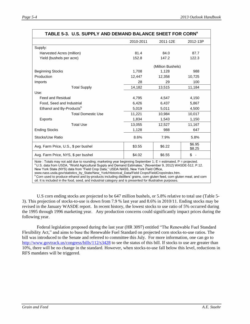
Page 5-4 2013 Outlook Handbook
Grain and Feed A.E. Staehr
TABLE 5-3. U.S. SUPPLY AND DEMAND BALANCE SHEET FOR CORNa
2010-2011 2011-12E 2012-13P
Supply:
Harvested Acres (million) 81.4 84.0 87.7
Yield (bushels per acre) 152.8 147.2 122.3
(Million Bushels)
Beginning Stocks 1,708 1,128 988
Production 12,447 12,358 10,725
Imports 28 29 100
Total Supply 14,182 13,515 11,184
Use:
Feed and Residual 4,795 4,547 4,150
Food, Seed and Industrial 6,426 6,437 5,867
Ethanol and By-Productsb 5,019 5,011 4,500
Total Domestic Use 11,221 10,984 10,017
Exports 1,834 1,543 1,150
Total Use 13,055 12,527 11,167
Ending Stocks 1,128 988 647
Stocks/Use Ratio 8.6% 7.9% 5.8%
Avg. Farm Price, U.S., $ per bushel $3.55 $6.22 $6.95 $8.25
Avg. Farm Price, NYS, $ per bushel $4.02 $6.55 $ -
Note : Totals may not add due to rounding; marketing year beginning September 1; E = estimated, P = projected. a U.S. data from USDA, “World Agricultural Supply and Demand Estimates,” (November 9, 2012) WASDE-512, P.12.
New York State (NYS) data from “Field Crop Data,” USDA NASS, New York Field Office, www.nass.usda.gov/statistics_by_State/New_York/Historical_Data/Field Crops/FieldCropsIndex.htm. b Corn used to produce ethanol and by-products including distillers’ grains, corn gluten feed, corn gluten meal, and corn
oil. It is included in the food, seed, and industrial category and is presented for illustrative purposes.
U.S corn ending stocks are projected to be 647 million bushels, or 5.8% relative to total use (Table 5-
3). This projection of stocks-to-use is down from 7.9 % last year and 8.6% in 2010/11. Ending stocks may be
revised in the January WASDE report. In recent history, the lowest stocks to use ratio of 5% occurred during
the 1995 through 1996 marketing year. Any production concerns could significantly impact prices during the
following year.
Federal legislation proposed during the last year (HR 3097) entitled “The Renewable Fuel Standard
Flexibility Act,” and aims to base the Renewable Fuel Standard on projected corn stocks-to-use ratios. The
bill was introduced to the Senate and referred to committee this July. For more information, one can go to
http://www.govtrack.us/congress/bills/112/s3428 to see the status of this bill. If stocks to use are greater than
10%, there will be no change in the standard. However, when stocks-to-use fall below this level, reductions in
RFS mandates will be triggered.

2013 Outlook Handbook Page 5-5
A.E. Staehr Grain and Feed
A way to combine supply and demand is to plot the stocks-to-use ratio against the average farm price
of corn for the year (Figure 5-1). The observations for 1989/90 through 2005/06 have a constant relationship
(i.e., the lower collection of points on the figure and estimated solid trend line). During this time, the demand
for corn was growing, but supply growth was keeping up with the demand; hence, the mean price over those
years was stable. A small upward shift is observable in 2006/07, followed by larger shifts in 2007/08 through
2009/10. The 2012/2013P combination represents another sizable price jump. Some may make the case that
we are now in a new plateau of prices; i.e., the mean has shifted (and represented by the dashed line).
However, a case was made in the mid 1990’s that corn prices would remain at high levels, only to
significantly decline when production and world economic factors changed. This graph illustrates how
relatively small changes in supply can affect price movement.
1.50
2.50
3.50
4.50
5.50
6.50
7.50
0 5 10 15 20 25 30
U.S. Averag e Farm Price, $'s per Bushel
Stocks to Use Ratio (%)
FIGURE 5 - 1. HISTORICAL RELATIONSHIP BETWEEN CORN
PRICES AND THE STOCKS - TO - USE RATIO, 1989 - 2012.
09/10
10/11
08/09 07/08
06/07
11/12E
12/13P

Page 5-6 2013 Outlook Handbook
Grain and Feed A.E. Staehr
The USDA Foreign Agricultural Service increased total world coarse grain production slightly from
October to November. Ending stocks were increased from 146.316 million metric tons in October to 147.075
million metric tons in November. Despite increased production prospects, this is still below last year’s total
production of 1.151 billion metric tons (Table 5-4A). Production increases in China, Argentina, and Mexico
partially offset decreases in other countries.
The world’s use and stock balances for corn are summarized in Table 5-4. Total use is projected to be
over 853.29 million metric tons in 2012/13. This is a 3.1% decrease over the previous year, but is still above
levels used during 2010 through 2011. As incomes in developing countries rise, demand for food increases.
The variation in ending stocks in recent years is an indicator of the ability of supply to balance use. Indicative
of low U.S. stocks, a world stocks-to-use ratio of 13.7% is projected for 2012/13 -- a lower level in recent
history not seen since the level observed in 2006/07.
TABLE 5-4A . WORLD COARSE GRAINS PRODUCTION
In Thousand Metric Tons
2008/09 2009/10 2010/11 2011/12 2012/13Oct 2012/13Nov
Production
Argentina 19,634 30,231 33,258 30,105 39,052 39,352
Australia 12,280 10,920 11,472 12,905 11,422 11,422
Brazil 53,486 58,412 60,380 75,883 73,493 73,493
Canada 27,184 22,477 22,263 21,831 23,635 23,635
China 172,391 169,775 183,398 199,660 207,010 207,010
Ethiopia 9,034 8,046 10,469 11,435 11,330 11,330
EU-27 162,102 155,038 140,497 147,149 140,995 140,276
India 39,550 33,890 43,370 42,060 37,610 37,610
Indonesia 8,700 6,900 6,800 8,900 8,500 8,900
Mexico 32,222 27,273 29,226 25,707 28,978 27,778
Nigeria 26,670 23,250 23,250 23,800 24,010 24,010
Russia 40,881 31,843 16,416 32,796 27,850 28,350
South Africa 13,084 13,881 11,321 12,497 13,973 13,973
Turkey 10,408 11,176 10,185 11,275 10,175 10,575
Ukraine 26,275 24,143 21,442 33,336 29,060 29,060
Others 131,832 137,277 143,946 138,203 138,794 139,394
Subtotal 785,733 764,532 767,693 827,542 825,887 826,168
United States 325,867 348,755 330,236 323,697 284,240 284,840
World Total 1,111,600 1,113,287 1,097,929 1,151,239 1,110,127 1,111,008 Source: USDA Foreign Agricultural Service

2013 Outlook Handbook Page 5-7
A.E. Staehr Grain and Feed
TABLE 5-4. WORLD SUPPLY-DEMAND BALANCE FOR CORN, 2005-06 to 2012-13a
Marketing Year Domestic
Use Ending Stocks
Stocks/ Use Ratio
(Million Metric Tons) (%)
2005 – 06 704.03 123.02 17.5%
2006 – 07 728.53 108.69 14.9
2007 – 08 771.23 129.72 16.8
2008– 09 781.10 147.99 18.9
2009 – 10 822.76 144.05 17.5
2010 – 11 849.24 127.00 14.9
2011 – 12E 880.49 132.08 15.0
2012 – 13P 853.29 117.27 13.7
aData from USDA, “World Agricultural Supply and Demand Estimates”. Various issues; E = estimated, P = projected
Price quotations for corn futures for nearby and distant contracts, as of 28 November 2012, help
summarize the current situation (Table 5-5). Research suggests that these prices are an adequate forecast as
any alternative, but like all forecasts, the futures quotes are imprecise, especially for the more distant time
periods. Clearly market expectations are bullish for the nearby months; however, going out one year, corn is
expected to be $1.21 per bushel lower than today, and corn for delivery in December 2014 is expected to be
$1.59 lower when compared to corn for delivery this year. Acres planted to corn this spring were at record
levels, and for spring 2013, high prices will be a major influence on planting decisions. The market is
expecting an increase in production, and there is limited incentive for farmers to store grain. Price differences
in the current month, compared to future months do not warrant storing grain until summer.
Since the USDA November report release, corn prices have come down marginally, but remain
highly variable from day to day. In summary, look for continued tight supply-demand conditions and
historically high feed grain prices at least through July 2013, with a necessity to replenish stocks amid strong
competition for crop acres. Concerns about sufficient U.S. corn supplies will make production risks from
weather increasingly problematic. Price volatility will be on continued high alert until an ample crop is
confirmed next year.

Page 5-8 2013 Outlook Handbook
Grain and Feed A.E. Staehr
TABLE 5-5. FUTURES PRICES FOR CORN,
CHICAGO MERCANTILE EXCHANGE, 28 NOVEMBER 2012
Contract Month - $ per bushel-
December 2012 $7.602
March 2013 7.640
May 2013 7.610
July 2013 7.530
September 2013 6.606
December 2013 6.396
December 2014 6.016
Soybeans
Current crop soybean projections were increased by 111 million bushels in the November crop report,
when compared to October. Soybean imports are expected to be 4 million bushels greater this year, compared
to last year. However, projected exports were raised by 80 million bushels in the November crop report
relative to the October report. Although harvested acres increased over last year, total supply decreased,
owing to a persistent drought in the Midwest and other areas. The supply and demand balance sheet for
soybeans is summarized in Table 5-6. An increase in harvested acres by 1.9 million acres was not enough to
offset a 2.6 bushel per acre decrease in yield. Weather stress at pod filling time contributed to lower yields,
with estimated U.S. production in 2012/13 reduced to 2.97 bb, a 3.97% reduction from 2011/12. Continued
reductions in projected crop production, combined with lower beginning stocks from year-ago levels imply a
total supply for 2012/13 of 3.021 bb, off 4.2% from last year.
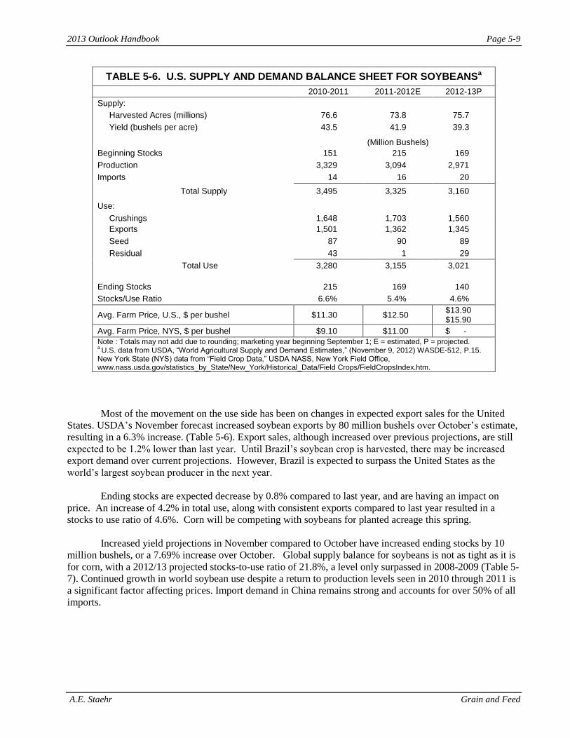
2013 Outlook Handbook Page 5-9
A.E. Staehr Grain and Feed
TABLE 5-6. U.S. SUPPLY AND DEMAND BALANCE SHEET FOR SOYBEANSa
2010-2011 2011-2012E 2012-13P
Supply:
Harvested Acres (millions) 76.6 73.8 75.7
Yield (bushels per acre) 43.5 41.9 39.3
(Million Bushels)
Beginning Stocks 151 215 169
Production 3,329 3,094 2,971
Imports 14 16 20
Total Supply 3,495 3,325 3,160
Use:
Crushings 1,648 1,703 1,560
Exports 1,501 1,362 1,345
Seed 87 90 89
Residual 43 1 29
Total Use 3,280 3,155 3,021
Ending Stocks 215 169 140
Stocks/Use Ratio 6.6% 5.4% 4.6%
Avg. Farm Price, U.S., $ per bushel $11.30 $12.50 $13.90 $15.90
Avg. Farm Price, NYS, $ per bushel $9.10 $11.00 $ -
Note : Totals may not add due to rounding; marketing year beginning September 1; E = estimated, P = projected. a U.S. data from USDA, “World Agricultural Supply and Demand Estimates,” (November 9, 2012) WASDE-512, P.15.
New York State (NYS) data from “Field Crop Data,” USDA NASS, New York Field Office, www.nass.usda.gov/statistics_by_State/New_York/Historical_Data/Field Crops/FieldCropsIndex.htm.
Most of the movement on the use side has been on changes in expected export sales for the United
States. USDA’s November forecast increased soybean exports by 80 million bushels over October’s estimate,
resulting in a 6.3% increase. (Table 5-6). Export sales, although increased over previous projections, are still
expected to be 1.2% lower than last year. Until Brazil’s soybean crop is harvested, there may be increased
export demand over current projections. However, Brazil is expected to surpass the United States as the
world’s largest soybean producer in the next year.
Ending stocks are expected decrease by 0.8% compared to last year, and are having an impact on
price. An increase of 4.2% in total use, along with consistent exports compared to last year resulted in a
stocks to use ratio of 4.6%. Corn will be competing with soybeans for planted acreage this spring.
Increased yield projections in November compared to October have increased ending stocks by 10
million bushels, or a 7.69% increase over October. Global supply balance for soybeans is not as tight as it is
for corn, with a 2012/13 projected stocks-to-use ratio of 21.8%, a level only surpassed in 2008-2009 (Table 5-
7). Continued growth in world soybean use despite a return to production levels seen in 2010 through 2011 is
a significant factor affecting prices. Import demand in China remains strong and accounts for over 50% of all
imports.

Page 5-10 2013 Outlook Handbook
Grain and Feed A.E. Staehr
TABLE 5-7. WORLD SUPPLY-DEMAND BALANCE FOR SOYBEANS, 2005-06 to 2012-13a
Marketing Year Domestic
Use Ending Stocks
Stocks/ Use Ratio
(Million Metric Tons) (%)
2005-06
215.21
52.94
24.6%
2006 – 07 225.28 62.68 27.8
2007 - 08 229.75 52.91 23.0
2008 – 09 221.13 44.02 19.9
2009-2010 238.22 59.41 24.9
2010 – 11 251.51 70.44 28.0
2011– 12E 239.22 56.00 23.4
2012 – 13P 264.28 57.56 21.8
aData from USDA, “World Agricultural Supply and Demand Estimates”. Various issues; E = estimated, P = projected
Average farm prices are projected to be higher than last year, with a forecasted range between $13.90
and $15.90 per bushel. While prices have moderated more recently, soybeans remain in a tenuously high price
position, even relative to a new higher level of prices over the past few years. Given expectations for future
supply, the market is expecting year-over-year decreases in futures commodity prices for beans and meal
(Table 5-8). Last year at this time, January contracts were trading about $2.78 per bu. lower for beans and
were over $102 per ton lower for meal. Since contracts for delivery in subsequent crop years are trading
below prices than for current delivery, the implication is that markets are expecting increased production over
the current crop year.
Uncertainty regarding potential policy changes relative to biofuels production will also be on the
radar in soybean markets. The U.S. Renewable Fuels Standard includes mandates of minimum volumes of
certain types of biofuels, e.g., conventional ethanol, biodiesel, and cellulosic ethanol. The total mandate
increases to 36 billion gallons (bg) in 2022, with increasing submandated usage of at least 1 bg of biodiesel
and 16 bg of biofuels from cellulosic biomass (both considered advanced biofuels). If the Administrator of the
Environmental Protection Agency, after consultation with the Secretary of Agriculture, determines that the
“implementation of the requirement would severely harm the economy or environment,” he/she can waive
part or the entire mandate. Waivers have already been granted on the cellulosic mandate, but the volumes
were negligible in the first two years minimal impact was realized from the decisions.

2013 Outlook Handbook Page 5-11
A.E. Staehr Grain and Feed
TABLE 5-8. FUTURES PRICES FOR SOYBEANS AND SOYBEAN MEAL, CHICAGO MERCANTILE EXCHANGE, 28 NOVEMBER 2012
Contract Month Beans Meal
$ per Bushel $ per Ton
January 2013 $14.462 $432.7
March 2013 14..350 425.3
May 2013 14.104 411.7
July 2013 13.776 405.9
September 2013 13.406 386.2
November 2013 13.050 367.7 (Dec 2013)
November 2014 12.774 360.6 (Dec 2014)
Future waivers under larger volumes may very well influence grain and oilseed commodity prices,
particularly if intra-category adjustments in conventional and advanced mandate levels are considered.
Furthermore, biodiesel helps to meet the submandate for advanced biofuels, but other advanced biofuels do
not help to meet the biodiesel mandate. Particular adjustments in biodiesel mandates may result in further
adjustments in commodity prices for oilseeds.
Feeds
Reduced production estimates for major feed commodities have increased prices for feed inputs and
reduced livestock margins. According to ERS data, consumer meat prices are expected to increase over the
next year. Beef prices increased 0.5 percent in October, resulting in a 5.5% increase over last October. ERS
predicts that consumer beef prices this year will be 5.5 to 6.5% higher than last year. Consumer poultry
prices increased 1.5% in October and are now 5.5% above last year’s prices.
Domestic feed grain utilization in 2012/13 is projected 5.9% below last season, a result of reduced
grain feeding in the face of record prices. Both beef and broiler animal product production is expected down
in 2013 (-4.2% and -1.2%, respectively) from 2012 estimated levels. Pork production is forecast lower in
early 2013 compared with 2012, down 1.4%. Projected milk production in 2013 is expected to be at the same
level as 2012, suggesting a limited impact on grain consumption for dairy. However, total red meat and
poultry exports are predicted to drop by 4.2% compared to last year.
Corn and soybean meal futures prices as of 28 November 2012 (Tables 5-5 and 5-8) are used, along
with other information, in a model to project selected mixed feed costs. One set of estimates for dairy, hog,
and layer feeds over the next year is shown in Table 5-9. They suggest, for example, that 18% protein dairy
feed could be about $20 per ton lower this coming spring than a year earlier. Hog feed costs are forecast to
drop $50 per ton while layer feed costs are forecast to decline $12 per ton.
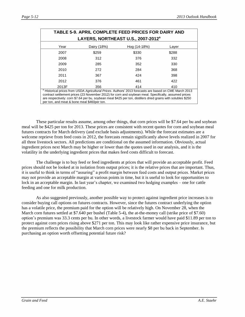
Page 5-12 2013 Outlook Handbook
Grain and Feed A.E. Staehr
TABLE 5-9. APRIL COMPLETE FEED PRICES FOR DAIRY AND
LAYERS, NORTHEAST U.S., 2007-2012a
Year Dairy (18%) Hog (14-18%) Layer
2007 $259 $330 $288
2008 312 376 332
2009 285 352 330
2010 272 284 368
2011 367 424 398 2012 376 461 422
2013F 356 414 410 a Historical prices from USDA Agricultural Prices. Authors’ 2013 forecasts are based on CME March 2013
contract settlement prices (23 November 2012) for corn and soybean meal. Specifically, assumed prices are respectively: corn $7.64 per bu, soybean meal $425 per ton, distillers dried grains with solubles $250 per ton, and meat & bone meal $460per ton.
These particular results assume, among other things, that corn prices will be $7.64 per bu and soybean
meal will be $425 per ton for 2013. These prices are consistent with recent quotes for corn and soybean meal
futures contracts for March delivery (and exclude basis adjustments). While the forecast estimates are a
welcome reprieve from feed costs in 2012, the forecasts remain significantly above levels realized in 2007 for
all three livestock sectors. All predictions are conditional on the assumed information. Obviously, actual
ingredient prices next March may be higher or lower than the quotes used in our analysis, and it is the
volatility in the underlying ingredient prices that makes feed costs difficult to forecast.
The challenge is to buy feed or feed ingredients at prices that will provide an acceptable profit. Feed
prices should not be looked at in isolation from output prices; it is the relative prices that are important. Thus,
it is useful to think in terms of “assuring” a profit margin between feed costs and output prices. Market prices
may not provide an acceptable margin at various points in time, but it is useful to look for opportunities to
lock in an acceptable margin. In last year’s chapter, we examined two hedging examples – one for cattle
feeding and one for milk production.
As also suggested previously, another possible way to protect against ingredient price increases is to
consider buying call options on futures contracts. However, since the futures contract underlying the option
has a volatile price, the premium paid for the option will be relatively high. On November 28, when the
March corn futures settled at $7.640 per bushel (Table 5-4), the at-the-money call (strike price of $7.60)
option’s premium was 33.3 cents per bu. In other words, a livestock farmer would have paid $11.89 per ton to
protect against corn prices rising above $271 per ton. This may look like rather expensive price insurance, but
the premium reflects the possibility that March corn prices were nearly $8 per bu back in September. Is
purchasing an option worth offsetting potential future risk?

Chapter 6. Dairy — Markets and PolicyMark W. Stephenson, Director of Dairy Policy Analysis
University of Wisconsin–Madison!
2013 Dairy Outlook
Positive Factors:• High levels of exports• Modest increase in U.S. milk supplies• Continued recovery of U.S. economy
Negative Factors:• Continued dry weather conditions across much of the U.S.• High feed prices• Substantial increase in Oceania milk production
Uncertainties:• Drought • World economy influenced by the European Union• Dairy Policies in a new Farm Bill
a Northeast federal order statistical uniform price for farms shipping milk to Suffolk County, MA (Boston).
Percent ChangeItem 2011 2012 2013 11-12 12-13
Number of milk cows (thousand head) 610 610 610 0.0 0.0
Milk per cow (lbs.) 21,026 21,590 21,967 2.4 2.0
Total milk production (million lbs.) 12,826 13,170 13,400 2.4 2.0
Blended milk price ($/cwt.) 20.64 18.74 20.40 -9.2 8.9
New York Dairy Situation and Outlook2011, Projected 2012, and Estimated 2013
a

2013 Outlook Handbook Page 6-2
M.W. Stephenson Dairy—Markets & Policy
Sour
ce:
Dai
ry S
ituat
ion
and
Out
look
, Milk
Pro
duct
ion,
and
Dai
ry M
arke
t New
s, U
.S. D
epar
tmen
t of A
gric
ultu
re.
Not
e th
at to
tal m
ay n
ot a
dd e
xact
ly
due
to ro
undi
ng.
* Le
ap y
ear.
a Rev
ised.
b Bas
ed o
n pr
elim
inar
y U
SDA
data
and
Cor
nell
estim
ates
.
Tabl
e 6-
1. U
.S. M
ilk S
uppl
y an
d U
tiliz
atio
n, 2
004
- 201
3
2004
2005
2006
2007
2008
2009
2010
2011
2012
*20
13
Sup
ply
Cow
s N
umbe
rs (t
hous
.)9,
011
9,04
39,
137
9,18
99,
315
9,20
39,
119
9,19
49,
237
9,22
1P
rodu
ctio
n/co
w (l
bs)
18,9
6819
,566
19,8
9420
,204
20,3
9620
,572
21,1
4821
,346
21,6
5121
,880
Pro
duct
ion
170.
917
6.9
181.
818
5.7
190.
018
9.3
192.
819
6.3
200.
020
1.8
Farm
Use
1.0
1.0
1.0
1.0
1.0
1.0
1.0
1.0
0.9
0.9
Mar
ketin
gs16
9.9
175.
918
0.8
184.
618
9.0
188.
419
1.9
195.
319
9.1
200.
8
Beg
inni
ng C
omm
erci
al S
tock
s8.
37.
28.
09.
510
.410
.011
.310
.911
.011
.3Im
ports
5.3
5.1
5.0
4.6
3.9
4.1
3.1
3.1
3.6
3.6
Tota
l Sup
ply
183.
618
8.2
193.
819
8.8
203.
320
2.5
206.
320
9.3
213.
621
5.7
Util
izat
ion
Com
mer
cial
Dis
appe
aran
ce17
6.5
180.
218
4.2
188.
419
3.2
190.
419
5.2
198.
320
2.3
206.
4E
ndin
g C
omm
erci
al S
tock
s7.
28.
09.
510
.410
.011
.310
.911
.011
.39.
3D
EIP
0.1
0.0
0.0
0.0
0.0
0.0
0.0
0.0
0.0
0.0
Net
Rem
oval
s (e
xclu
ding
DE
IP)
-0.2
0.0
0.0
0.0
0.0
0.7
0.2
0.0
0.0
0.0
Tota
l Use
183.
618
8.2
193.
819
8.8
203.
320
2.5
206.
320
9.3
213.
621
5.7
* a
* b
c

The Dairy Situation
For dairy producers 2010 and 2011 were recovery years from the recession and low milk prices of 2009. The 2012 milk price declined by about two dollars per hundredweight from the all-time high average price of 2011, but producers might characterize 2012 as a “disastrous year” or a “middling year” depending on their business model or their geographic location. Milk production in New Zealand and widespread drought in the U.S. have really defined this year for the U.S. dairy industry.
The Drought
The related, but very different, weather patterns of La Niña and El Niño were both a part of the 2012 story. We have had a couple of years of La Niña which is a colder body of water in the equatorial Pacific. This tends to create warmer and drier weather in the central portion of the U.S. In fact, the drought here was widespread and one of the worst that we have seen causing significant loss of crops throughout the central portion of the country. Dairy farms located within drought-affected areas experienced outcomes which ranged from total crop loss to greatly reduced yields. All dairy farms have experienced significantly higher purchased feed costs, but if your business model is one which depends on both purchased concentrates and forages, the milk price may not have been adequate to cover your variable costs of production.
Figure 1. U.S. Drought Monitor, November 27, 2012.
2013 Outlook Handbook Page 6-3
M.W. Stephenson Dairy—Markets & Policy

La Niña also affects the other side of the Pacific by bringing higher-than-normal rains to Oceania. New Zealand has benefited from excellent pastures both last year and in the 2011-12 season. They increased milk production 10.43% in 2011 and are on track to increase just less than 5% this year. New Zealand production is important to the U.S. dairy industry because they compete for the same export markets that we do. New Zealand production impacts U.S. milk prices just as U.S. production now impacts New Zealand milk prices.
El Niño is a warmer-than-normal body of water in the equatorial Pacific ocean and it typically brings greater quantities of rain to the western U.S. and drier weather conditions to Oceania. El Niño was expected to form this summer bringing needed rains to relieve the U.S. drought and it would have been expected to worsen the pasture conditions in New Zealand. However, the El Niño did not form and the National Oceanic and Atmospheric Administration does not expect one in the year ahead.
$0
$2
$4
$6
$8
$10
$12
$14
2000
2001
2002
2003
2004
2005
2006
2007
2008
2009
2010
2011
2012
Hay Value Soybean Value Corn Value
Figure 2. NASS Value of the Dairy Ration.
There was little direct impact of the drought on the traditional dairy regions in the Northeast. Drought impacts varied in Midwest from severe on farms in southern Wisconsin, northern Illinois, and in Minnesota and Iowa. But many farms outside these areas were largely spared or even had excellent crop yields. Even the farms that were impacted may have had lower quantity but the quality of the forages were quite good. However, the price of feed was heavily impacted in all parts of the country.
Western dairy business models where all feeds are purchased and where the feed basis is higher than in the Midwest, have suffered substantially. This is evidenced by the milk production reports in the last quarter of 2012. For example, September and October milk production in California declined by
2013 Outlook Handbook Page 6-4
M.W. Stephenson Dairy—Markets & Policy

3.9% and 3.5% respectively while Wisconsin milk production increased by 3.5% and 4.7% in those same months.
Dairy Product Demand
Unemployment has remained stubbornly high following the recession in 2009. However, there has been some evidence of optimism on the part of consumers as evidenced by increases in the purchase of durable goods and other measures of consumer sentiment. In fact, retail dairy prices have not increased more rapidly than other food or the general economy. Per capita consumption of most dairy products has increased with the yogurt category a particularly bright spot. However, beverage milk is the negative exception to most dairy products and created headlines for dropping below a threshold of 20 gallons per capita.
130
135
140
145
150
155
160
Jan-
08
Apr
-08
Jul-0
8
Oct
-08
Jan-
09
Apr
-09
Jul-0
9
Oct
-09
Jan-
10
Apr
-10
Jul-1
0
Oct
-10
Jan-
11
Apr
-11
Jul-1
1
Oct
-11
Jan-
12
Apr
-12
Jul-1
2
Mill
ions
of P
ound
s
Figure 3. U.S. Average Daily Sales of Fluid Milk.
Dairy Exports
The U.S. continues to solidify it’s place as a major world dairy product exporter. The European Union and New Zealand are essentially tied with 35% and 34% shares of world trade respectively. The U.S. comes in at third place with about a 19% share of world exports. Australia is the forth largest exporter with 7% of the trade share.
Nonfat Dry Milk or Skim Milk powder is the largest volume of U.S. export followed closely by dry whey products. Lactose, cheese and butter round out the remaining bulk of export products. From January, 2012 through September, 2012, the milk solids exported represent about 13.6% of the total milk solids produced.
2013 Outlook Handbook Page 6-5
M.W. Stephenson Dairy—Markets & Policy
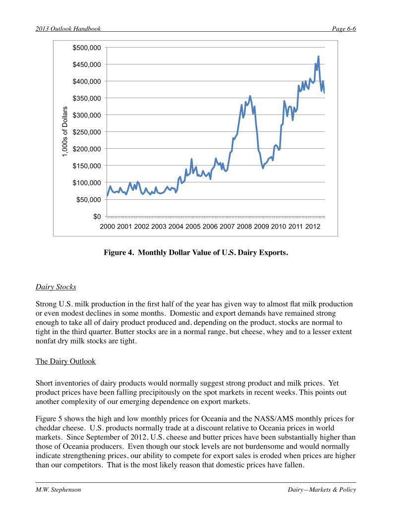
$0
$50,000
$100,000
$150,000
$200,000
$250,000
$300,000
$350,000
$400,000
$450,000
$500,000
2000 2001 2002 2003 2004 2005 2006 2007 2008 2009 2010 2011 2012
1,00
0s o
f Dol
lars
Figure 4. Monthly Dollar Value of U.S. Dairy Exports.
Dairy Stocks
Strong U.S. milk production in the first half of the year has given way to almost flat milk production or even modest declines in some months. Domestic and export demands have remained strong enough to take all of dairy product produced and, depending on the product, stocks are normal to tight in the third quarter. Butter stocks are in a normal range, but cheese, whey and to a lesser extent nonfat dry milk stocks are tight.
The Dairy Outlook
Short inventories of dairy products would normally suggest strong product and milk prices. Yet product prices have been falling precipitously on the spot markets in recent weeks. This points out another complexity of our emerging dependence on export markets.
Figure 5 shows the high and low monthly prices for Oceania and the NASS/AMS monthly prices for cheddar cheese. U.S. products normally trade at a discount relative to Oceania prices in world markets. Since September of 2012, U.S. cheese and butter prices have been substantially higher than those of Oceania producers. Even though our stock levels are not burdensome and would normally indicate strengthening prices, our ability to compete for export sales is eroded when prices are higher than our competitors. That is the most likely reason that domestic prices have fallen.
2013 Outlook Handbook Page 6-6
M.W. Stephenson Dairy—Markets & Policy

$1.00
$1.20
$1.40
$1.60
$1.80
$2.00
$2.20
$2.40
$2.60
$2.80
Jan-
05
May
-05
Sep
-05
Jan-
06
May
-06
Sep
-06
Jan-
07
May
-07
Sep
-07
Jan-
08
May
-08
Sep
-08
Jan-
09
May
-09
Sep
-09
Jan-
10
May
-10
Sep
-10
Jan-
11
May
-11
Sep
-11
Jan-
12
May
-12
Sep
-12
Low
High
NASS
Figure 5. Oceania High and Low Cheese Prices, NASS/AMS Cheese Prices.
Oceania has very seasonal milk production and they are now several months past their peak lactation. World markets have absorbed the products during their flush and this is an indication of a robust demand for dairy products. It is likely that U.S. prices will not have much further to fall but rather that world prices will come up to meet our prices.
I am projecting a New York All Milk price to average about $20.75 in 2013. This would be an increase of about $1.35 from the 2012 levels. Moreover, the futures markets show a continual decline in soybean meal prices from now through the next harvest season representing a $70 drop. Corn prices are expected to remain at the current high levels until next harvest season when futures markets anticipate a decline of about $1 per bushel. The combination of increased milk price and an easing of feed prices would improve farm margins.
Dairy Policy
At the time of this writing, we are in the lame duck session of congress. Although Democrats picked up a few seats, the balance of power was not altered and a stalemate exists on most pieces of legislation. The Senate has passed their version of a farm bill and the House Agricultural Committee has reported their version out but it has not made it to the floor of the House for a vote. If the House moves on the farm bill before the end of the year, it is likely that the dairy provisions in the House and Senate (which are quite similar) will be the new policy for dairy.
2013 Outlook Handbook Page 6-7
M.W. Stephenson Dairy—Markets & Policy

The dairy provisions are a marked departure from previous policy. They would seek to find budget savings by eliminating the Dairy Product Price Support Program and the Milk Income Loss Contracts. These safety net programs would be replaced by a voluntary margin insurance program and a market stabilization program.
The most likely scenario for passage in the lame duck session is to attach the farm bill to whatever legislation may be passed to address the so-called “fiscal cliff”. If that doesn’t happen, then it is likely that congress would pass an extension of the previous farm bill until new legislation can be passed later on. This is a dangerous proposition for promoters of the current House and Senate bills.
By March, the Congressional Budget Office will have a new baseline against which all bills with fiscal consequences will be evaluated. Few believe that the new CBO baseline will look better than last year’s and most believe that it will look much worse. If that is true, then congress will have to go back and reconsider the proposed House and Senate farm bills and find new areas for cost saving. Opening up the bills to new scrutiny increases the likelihood that we could see substantial changes in any of the programs—including dairy.
Substantial changes in dairy policy are likely. But, what those changes will be and when they will take place is an unknown at this time.
2013 Outlook Handbook Page 6-8
M.W. Stephenson Dairy—Markets & Policy

Tabl
e 6-
2. N
atio
nal F
arm
Pric
es fo
r Milk
; CC
C P
urch
ase,
Who
lesa
le, a
nd R
etai
l Pric
es fo
r Che
ddar
Che
ese,
But
ter,
and
Non
fat D
ry M
ilk; a
nd S
elec
ted
Ret
ail P
rice
Indi
ces,
200
2–20
12
2002
2003
2004
2005
2006
2007
2008
2009
2010
2011
2012
Farm
Milk
($/c
wt.)
All
Milk
(ave
. fat
)12
.18
12.5
516
.05
15.1
312
.88
19.1
318
.33
12.8
216
.26
20.1
418
.54
Cla
ss II
I (3.
5%)
10.4
211
.42
15.3
914
.05
11.8
918
.04
17.4
411
.36
14.4
018
.37
17.5
7S
uppo
rt (3
.5%
)9.
809.
809.
809.
809.
809.
809.
809.
809.
809.
809.
80M
ilk P
rice:
Fee
d P
rice
Valu
e2.
602.
613.
103.
242.
572.
812.
011.
782.
261.
881.
52M
ILC
pay
men
ts1.
211.
090.
220.
010.
610.
010.
001.
150.
020.
000.
68
Che
ddar
Che
ese,
Blo
cks
($/lb
.)C
CC
Pur
chas
e1.
131
1.13
11.
131
1.13
11.
131
1.13
11.
131
1.13
01.
130
1.13
01.
130
Who
lesa
le, C
hica
go M
erca
ntile
Exc
hang
e1.
182
1.31
71.
649
1.49
21.
239
1.75
81.
856
1.29
61.
496
1.80
61.
727
But
ter (
$/lb
.)C
CC
Pur
chas
e, G
rade
A o
r hig
her,
Chi
cago
0.85
51.
050
1.05
01.
050
1.05
01.
050
1.05
01.
050
1.05
01.
050
1.05
0W
hole
sale
, Gr.
AA
, Chi
cago
Mer
c. E
xcha
nge
1.10
61.
145
1.81
71.
549
1.23
61.
368
1.46
51.
243
1.72
81.
962
1.63
7
Non
fat D
ry M
ilkC
CC
Pur
chas
e, U
nfor
tifie
d ($
/lb.)
0.90
00.
800
0.80
00.
800
0.80
00.
800
0.80
00.
800
0.80
00.
800
0.80
0W
hole
sale
, Cen
tral S
tate
s0.
928
0.83
80.
858
0.98
51.
001
1.80
41.
300
1.01
01.
247
1.56
41.
375
Ret
ail P
rice
Indi
ces
(198
2–84
=100
.0)
2002
2003
2004
2005
Milk
110.
611
1.5
125.
012
7.0
125.
514
0.1
148.
512
9.0
133.
614
5.8
146.
7C
hees
e17
0.0
169.
418
0.8
183.
318
0.8
191.
521
4.6
203.
520
4.8
217.
522
2.2
All
Dai
ry P
rodu
cts
168.
116
7.9
180.
218
2.4
181.
419
4.8
210.
419
7.0
199.
221
2.7
216.
9A
ll Fo
od17
6.2
180.
018
6.2
190.
719
5.2
202.
921
4.1
218.
021
9.7
227.
823
3.4
All
Con
sum
er P
rices
179.
918
4.0
188.
919
5.3
201.
620
7.3
215.
321
4.5
218.
122
4.9
229.
5
c
Sour
ce:
Dai
ry S
ituat
ion
and
Out
look
, Dai
ry M
arke
t New
s, an
d Fe
dera
l Milk
Ord
er M
arke
t Sta
tistic
s, U
.S. D
epar
tmen
t of A
gric
ultu
re.
a Re
vise
d.b
Estim
ated
by
Mar
k St
ephe
nson
.c
Milk
Inco
me
Loss
Con
tract
pay
men
ts be
gan
in O
ctob
er o
f 200
1.
2013 Outlook Handbook Page 6-9
M.W. Stephenson Dairy—Markets & Policy

Month 2011 2012 Difference
October 20.42 20.78 0.36November 20.23 21.78 1.55December 19.57 21.49 1.92Fourth Quarter Average 20.07 21.35 1.28
Annual Average 20.64 18.74 -1.91
Month 2012 2013 Difference
January 19.37 20.43 1.06February 18.09 20.42 2.33March 17.64 20.47 2.83First Quarter Average 18.37 20.44 2.07
April 17.20 20.50 3.30May 16.79 20.62 3.83June 16.58 20.67 4.09Second Quarter Average 16.86 20.60 3.74
July 17.26 20.66 3.40August 18.40 20.49 2.09September 19.45 20.38 0.93Third Quarter Average 18.37 20.51 2.14
October 20.78 20.18 -0.60November 21.78 20.11 -1.67December 21.49 19.81 -1.68Fourth Quarter Average 21.35 20.03 -1.32
Annual Average 18.74 20.40 1.66
(dollars per hundredweight)
(dollars per hundredweight)
MILK PRICE PROJECTIONS*Northeast Federal Order Statistical Uniform Price
3.5 Percent, Suffolk County, MassachusettsLast Quarter 2011-2012, Four Quarters 2012-2013
a!
a!
a!a!
a! a!
a!
a!
a!
a!a!a!
a!
a!a!
a!
a!a!a!
2013 Outlook Handbook Page 6-10
M.W. Stephenson Dairy—Markets & Policy
* Averages may not add due to rounding.a Projected.

W.A. Knoblauch/G.J. Conneman/L.D. Putnam Dairy--Farm Management
Chapter 7. Dairy -- Farm Management Wayne A. Knoblauch, Professor George J. Conneman, Professor
Linda D. Putnam, Extension Support Specialist
Herd Size Comparisons
The 190 New York dairy farms that participated in the Dairy Farm Business Summary (DFBS) Project in 2011 have been sorted into seven herd size categories and averages for the farms in each category are presented in Tables 7-1 and 7-2. Note that after the less than 60 cow category, the herd size categories increase by 40 cows up to 100 cows, by 100 cows up to 200 cows, by 200 cows up to 600 cows and by 300 cows up to 900 cows. In most years, as herd size increases, the net farm income increases; and that was the case for 2011 (Table 7-1). Net farm income without appreciation averaged $27,613 per farm for the less than 60 cow farms and $1,606,213 per farm for those with more than 900 cows. Return to all capital without appreciation generally increased as herd size increased. With herd sizes less than 200 cows, many farms find it difficult to find a low cost combination of technology and labor to produce milk. Thus profits are lower for these herds than other herd sizes. It is more than size of herd that determines profitability on dairy farms. The over 900 herd size category had the highest net farm income per cow at $1,189 while the under 60 herd size category had the lowest net farm income per cow at $608. In some years, other herd size categories have averaged the highest net farm income per cow. Other factors that affect profitability and their relationship to the size classifications are shown in Table 7-2.
TABLE 7-1. COWS PER FARM AND FARM FAMILY INCOME MEASURES 190 New York Dairy Farms, 2011
Number of Cows
Number
of Farms
Average Number
of Cows
Net Farm Income without
Appreciation
Net Farm Income per Cow
Labor & Management Income per Operator
Return to all Capital
without Appreciation
Under 60 20 45 $27,613 $608 $ -5,773 -2.0%
60 to 99 23 75 46,993 628 3,174 0.2%
100 to 199 30 142 132,825 836 40,182 5.1%
200 to 399 24 317 329,007 1,037 127,176 9.3%
400 to 599 26 506 564,133 1,114 184,927 11.0%
600 to 899 28 733 862,484 1,176 305,690 11.6%
900 & over 39 1,351 1,606,213 1,189 444,449 12.2%
Note: All data in this chapter are from the New York Dairy Farm Business Summary and Analysis Project unless a specific source is specified. Publications reporting Dairy Farm Business Summary data for New York, three regions of the state, for large herds, small herds, grazing farms, and farms that rent are available from the Charles H. Dyson School of Applied Economics and Management website: http://www.dyson.cornell.edu/outreach/index.php .

2013 Outlook Handbook
Dairy--Farm Management W.A. Knoblauch/G.J. Conneman/L.D. Putnam
Page 7-2
This year, net farm income per cow did generally exhibit the usual increase as herd size increased. All herd size categories saw an increase in operating cost of producing milk from a year earlier (Table 7-2). Net farm income per cow will increase as farms become larger if the costs of increased purchased inputs are offset by greater and more efficient output. The farms with more than 900 cows averaged more milk sold per cow than any other size category (Table 7-2). With 25,689 pounds of milk sold per cow, farms in the largest herd size group averaged 9.3 percent more milk output per cow than the average of all herds in the summary with less than 900 cows. The ability to reach high levels of milk output per cow with a large herd is a major key to profitability. Three times a day milking (3X) and supplementing with bST are herd management practices commonly used to increase milk output per cow in large herds. Many dairy farmers who have been willing and able to employ and manage the labor required to milk 3 times per day have been successful. Only 7 percent of the 43 DFBS farms with less than 100 cows used a milking frequency greater than 2 times per day. As herd size increased, the percent of herds using a higher milking frequency increased. Farms with 100 to 200 cows reported 13 percent of the herds milking more often than 2 times per day, the 200-399 cow herds reported 67 percent, 400-599 cow herds reported 62 percent, 600-899 cow herds reported 82 percent, and the 900 cow and larger herds reported 95 percent exceeding the 2 times per day milking frequency.
TABLE 7-2. COWS PER FARM AND RELATED FARM FACTORS 190 New York Dairy Farms, 2011
Number
Average Number
of
Milk Sold
Per Cow
Milk Sold Per Worker
Till- able
Acres
Forage DM Per
Cow
Farm Capital
Per
Cost of Producing Milk/Cwt.
of Cows Cows (lbs.) (cwt.) Per Cow (tons) Cow Operating Total
Under 60 45 17,158 4,213 3.6 7.4 $13,450 $15.71 $26.75
60 to 99 75 19,148 5,840 3.0 8.6 11,391 16.08 24.03
100 to 199 142 20,785 7,307 2.7 8.2 10,973 15.65 21.50
200 to 399 317 23,461 9,967 2.0 7.9 9,745 15.55 19.47
400 to 599 506 23,759 10,347 2.4 8.2 9,137 15.58 19.34
600 to 899 733 24,580 11,105 2.0 7.5 9,714 15.57 18.99
900 & over 1,351 25,689 11,738 1.9 7.4 9,470 15.72 18.87
Milk output per worker has always shown a strong correlation with herd size. The farms with 100 cows or more averaged over 1,111,879 pounds of milk sold per worker while the farms with less than 100 cows averaged less than 519,500 pounds per worker. In achieving the highest productivity per cow and per worker, the largest farms had the fewest crop acres per cow but also the lowest forage dry matter harvested per cow. The 400 to 599 herd size group had the more efficient use of farm capital with an average investment of $9,137 per cow. The 39 farms with 900 or more cows had the lowest total cost of producing milk at $18.87 per hundredweight. This is $0.74 below the $19.61 average for the remaining 151 dairy farms. The lower average costs of production plus a similar milk price gave the managers of these large dairy farms profit margins (milk price less total cost of producing milk) that averaged $0.70 per hundredweight above the average of the other 151 DFBS farms.

2013 Outlook Handbook
W.A. Knoblauch/G.J. Conneman/L.D. Putnam Dairy--Farm Management
Page 7-3
Dairy Operations and Milk Cow Inventory
TABLE 7-3. NUMBER OF DAIRY FARMS AND MILK COWS BY SIZE OF HERD New York State, 2011 a, b
Size of Herd
Farms
Milk Cows
Number of Cows
Number
% of Total
Number
% of Total
1 – 29
800
17.3%
8,000
1.3%
30 – 49
850
18.5%
30,000
4.9%
50 – 99
1,600
34.8%
120,000
19.7%
100 – 199
846
18.4%
108,000
17.7%
200 – 499
250
5.4%
80,000
13.1%
500 – 749
123
2.7%
76,000
12.5%
750 – 999
39
0.8%
34,000
5.6%
1,000 – 1,499
51
1.1%
63,000
10.3%
1,500 – 1,999
21
0.5%
36,000
5.9%
2,000 or more
20
0.5%
55,000
9.0%
Total
4,600
100.0%
610,000
100.0%
aThis information on number of farms and number of cows by size of herd is derived from several sources: - Dairy Statistics as published by the New York Agricultural Statistics Services for 2011. - CAFO (Concentrated Animal Feeding Operations) permit reports for 2011. Some small CAFO farms (farms with
200 plus milk cows) have not applied for or updated the permit. Estimates for these farms were made so as to reflect the total number of dairy farms in New York State; revision from Census in certain size categories.
b The author wishes to thank everyone who provided some data as well as providing valuable advice and perspectives. However, any errors, omissions or misstatements are solely the responsibility of the author, Professor George Conneman, e-mail [email protected].
In 2011, there were 4,600 dairy farms in New York State, and 610,000 milk cows. The table
above was prepared based on the NYASS data plus the CAFO permit filing for additional herd size categories.
Eighty-nine percent of the farms (less than 200 cows per farm) had 44 percent of the milk cows. The remaining eleven percent of the farms had 56 percent of the cows.
About 6 percent of the farms (those with 500 or more cows) had 43 percent of the cows.
Farms with less than 50 cows represent 36 percent of all farms but kept only 6 percent of the cows.
Farms with 1,000 or more cows (92 farms) represent about 2.0 percent of the farms but kept over 25 percent of the cows.
Ten-Year Comparisons
The total cost of producing milk on DFBS farms has increased $5.06 per hundredweight over the past 10 years (Table 7-4). In the intervening years, total cost of production increased in 2003 and 2004, decreased in 2005 and 2006, increased in 2007 and 2008, decreased in 2009, increased to $17.73 in 2010 and $19.92 in 2011. It is interesting to note that costs of production decrease in low milk price years and increase in high milk price years. Over the 10 years, milk sold per cow increased 10 percent and cows per worker increased 7 percent on DFBS farms (Table 7-5). Farm net worth has increased significantly, while percent equity has been fairly stable.

2013 Outlook Handbook
Dairy--Farm Management W.A. Knoblauch/G.J. Conneman/L.D. Putnam
Page 7-4
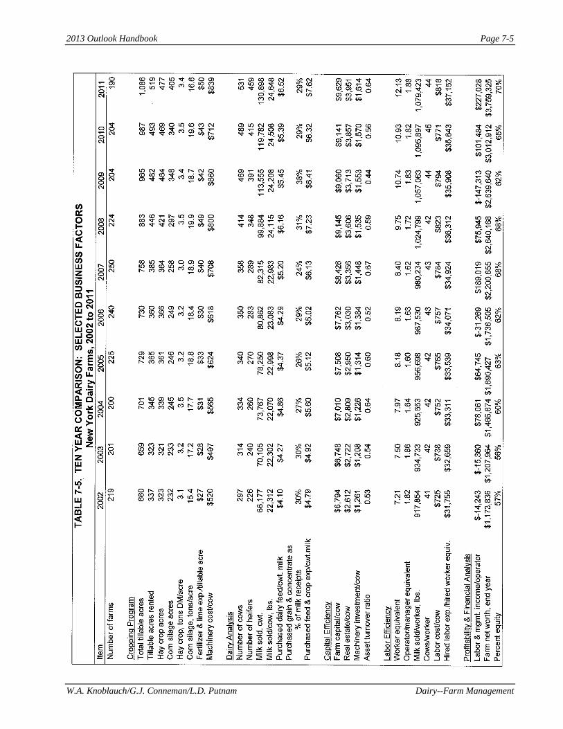
2013 Outlook Handbook
W.A. Knoblauch/G.J. Conneman/L.D. Putnam Dairy--Farm Management
Page 7-5

2013 Outlook Handbook
Dairy--Farm Management W.A. Knoblauch/G.J. Conneman/L.D. Putnam
Page 7-6
TABLE 7-6. COMPARISON OF FARM BUSINESS SUMMARY DATA Same 87 New York Dairy Farms, 2002 - 2011
Selected Factors
2002
2003
2004
2005
Milk receipts per cwt. milk $13.02 $13.28 $16.78 $16.05 Size of Business Average number of cows 375 394 420 436 Average number of heifers 286 302 315 341 Milk sold, cwt. 86,701 90,707 95,417 102,482 Worker equivalent 8.90 9.38 9.93 10.29 Total tillable acres 769 814 862 891 Rates of Production Milk sold per cow, lbs. 23,130 23,031 22,723 23,490 Hay DM per acre, tons 3.4 3.4 3.5 3.4 Corn silage per acre, tons 15 17 19 19 Labor Efficiency Cows per worker 42 42 42 42 Milk sold per worker, lbs. 974,167 967,029 960,901 995,939 Cost Control Grain & concentrate purchased as % of milk sales 29% 31% 27% 26% Dairy feed & crop expense per cwt. milk $4.72 $4.96 $5.55 $5.08 Operating cost of producing cwt. milk $10.79 $11.19 $12.20 $11.95 Total cost of producing cwt. milk $13.93 $14.20 $15.30 $15.20 Hired labor cost per cwt. $2.52 $2.56 $2.70 $2.64 Interest paid per cwt. $0.53 $0.49 $0.48 $0.57 Labor & machinery costs per cow $1,247 $1,244 $1,311 $1,371 Replacement livestock expense $12,138 $13,606 $17,175 $17,422 Expansion livestock expense $20,808 $14,513 $30,533 $15,372 Capital Efficiency Farm capital per cow $6,687 $6,682 $6,839 $7,404 Machinery & equipment per cow $1,223 $1,180 $1,188 $1,297 Real estate per cow $2,510 $2,580 $2,611 $2,756 Livestock investment per cow $1,782 $1,801 $1,832 $1,994 Asset turnover ratio 0.56 0.56 0.68 0.64 Profitability Net farm income without appreciation $70,144 $71,343 $307,034 $272,178 Net farm income with appreciation $137,988 $140,575 $422,365 $438,696 Labor & management income per operator/manager
$-4,378
$-6,801
$129,759
$93,626
Rate return on: Equity capital with appreciation 4.2% 4.1% 19.6% 17.2% All capital with appreciation 4.3% 4.1% 13.6% 12.9% All capital without appreciation 1.6% 1.5% 9.6% 7.7% Financial Summary, End Year Farm net worth $1,522,222 $1,587,206 $1,910,499 $2,234,618 Change in net worth with appreciation $11,878 $57,066 $316,467 $308,353 Debt to asset ratio 0.40 0.41 0.37 0.34 Farm debt per cow $2,679 $2,775 $2,608 $2,630 Farms participating in the DFBS each of the last 10 years have increased size of business, labor efficiency and milk sold per cow (Table 7-6). All measures of profitability exhibit wide variability from year-to-year and are highly correlated with milk price received.
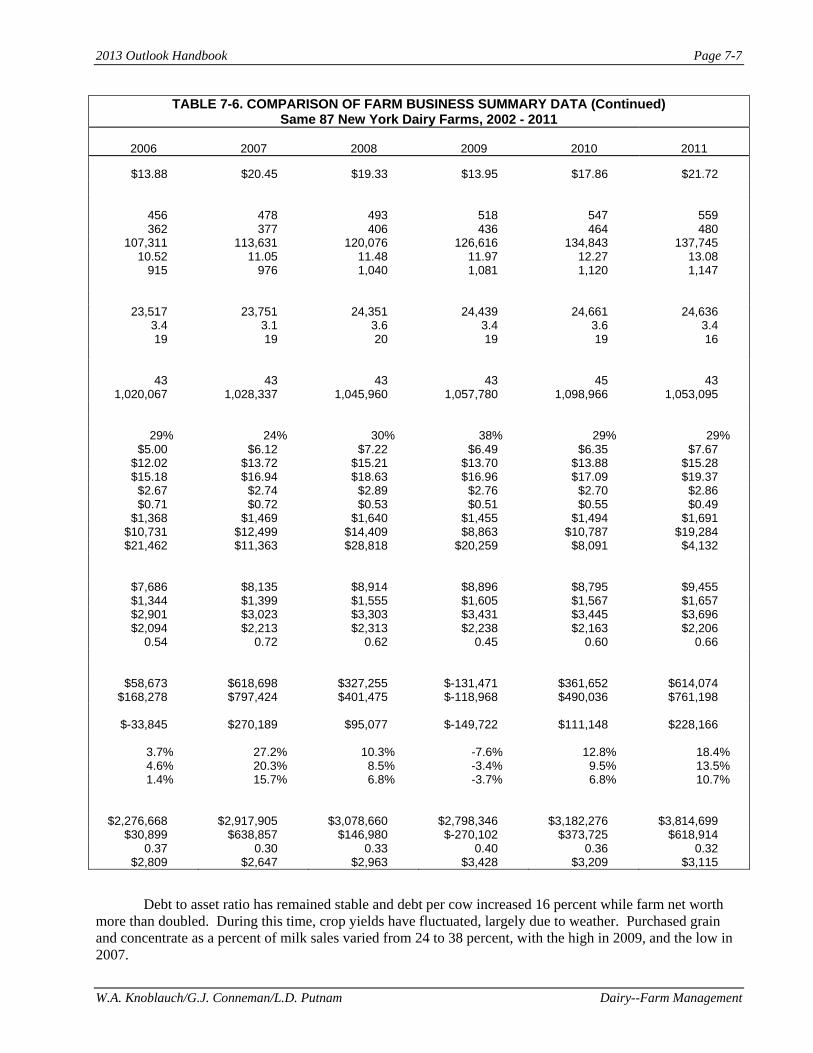
2013 Outlook Handbook
W.A. Knoblauch/G.J. Conneman/L.D. Putnam Dairy--Farm Management
Page 7-7
TABLE 7-6. COMPARISON OF FARM BUSINESS SUMMARY DATA (Continued) Same 87 New York Dairy Farms, 2002 - 2011
2006
2007
2008
2009
2010
2011
$13.88 $20.45 $19.33 $13.95 $17.86 $21.72
456 478 493 518 547 559 362 377 406 436 464 480
107,311 113,631 120,076 126,616 134,843 137,745 10.52 11.05 11.48 11.97 12.27 13.08
915 976 1,040 1,081 1,120 1,147
23,517 23,751 24,351 24,439 24,661 24,636 3.4 3.1 3.6 3.4 3.6 3.4 19 19 20 19 19 16
43 43 43 43 45 43 1,020,067 1,028,337 1,045,960 1,057,780 1,098,966 1,053,095
29% 24% 30% 38% 29% 29% $5.00 $6.12 $7.22 $6.49 $6.35 $7.67
$12.02 $13.72 $15.21 $13.70 $13.88 $15.28 $15.18 $16.94 $18.63 $16.96 $17.09 $19.37
$2.67 $2.74 $2.89 $2.76 $2.70 $2.86 $0.71 $0.72 $0.53 $0.51 $0.55 $0.49
$1,368 $1,469 $1,640 $1,455 $1,494 $1,691 $10,731 $12,499 $14,409 $8,863 $10,787 $19,284 $21,462 $11,363 $28,818 $20,259 $8,091 $4,132
$7,686 $8,135 $8,914 $8,896 $8,795 $9,455 $1,344 $1,399 $1,555 $1,605 $1,567 $1,657 $2,901 $3,023 $3,303 $3,431 $3,445 $3,696 $2,094 $2,213 $2,313 $2,238 $2,163 $2,206
0.54 0.72 0.62 0.45 0.60 0.66
$58,673 $618,698 $327,255 $-131,471 $361,652 $614,074 $168,278 $797,424 $401,475 $-118,968 $490,036 $761,198
$-33,845
$270,189
$95,077
$-149,722
$111,148
$228,166
3.7%
27.2%
10.3%
-7.6%
12.8%
18.4%
4.6% 20.3% 8.5% -3.4% 9.5% 13.5% 1.4% 15.7% 6.8% -3.7% 6.8% 10.7%
$2,276,668 $2,917,905 $3,078,660 $2,798,346 $3,182,276 $3,814,699 $30,899 $638,857 $146,980 $-270,102 $373,725 $618,914
0.37 0.30 0.33 0.40 0.36 0.32 $2,809 $2,647 $2,963 $3,428 $3,209 $3,115
Debt to asset ratio has remained stable and debt per cow increased 16 percent while farm net worth more than doubled. During this time, crop yields have fluctuated, largely due to weather. Purchased grain and concentrate as a percent of milk sales varied from 24 to 38 percent, with the high in 2009, and the low in 2007.

2013 Outlook Handbook
Dairy--Farm Management W.A. Knoblauch/G.J. Conneman/L.D. Putnam
Page 7-8
TABLE 7-7. COMPARISON OF DAIRY FARM BUSINESS DATA BY REGION 192 New York Dairy Farms, 2011
Item
Western & Central Plateau Region
Western & Central
Plain Region
Northern New York
Central Valleys
Northern Hudson &
SoutheasternNew York
Number of farms 33 57 25 31 46 ACCRUAL EXPENSES Hired labor $215,864 $503,502 $484,134 $295,066 $272,546 Feed 559,374 1,185,580 1,185,994 650,100 672,844 Machinery 183,802 356,303 440,651 266,790 228,541 Livestock 277,282 593,926 619,395 338,262 337,731 Crops 78,658 174,950 224,834 132,532 106,281 Real estate 83,864 154,175 147,520 96,619 77,628 Other 95,333 220,199 273,522 149,298 130,268 Total Operating Expenses $1,494,176 $3,188,635 $3,376,050 $1,928,667 $1,825,839 Expansion livestock 14,226 5,387 10,771 6,839 4,251 Extraordinary expense 99 0 288 2,877 0 Machinery depreciation 67,552 142,628 166,165 111,086 69,337 Building depreciation 40,415 107,047 109,739 58,055 37,249 Total Accrual Expenses $1,616,468 $3,443,698 $3,663,013 $2,107,523 $1,936,675 ACCRUAL RECEIPTS Milk sales $1,904,536 $3,707,509 $4,101,723 $2,445,843 $2,101,853 Livestock 132,333 287,287 268,280 144,243 145,003 Crops 15,452 67,146 111,423 30,852 45,340 Government receipts 8,608 25,785 11,488 14,451 15,461 All other 17,406 95,640 94,446 44,485 49,741 Total Accrual Receipts $2,078,336 $4,183,368 $4,587,360 $2,679,875 $2,357,397 PROFITABILITY ANALYSIS
Net farm income (w/o appreciation) $461,868 $739,670 $924,347 $572,352 $420,722 Net farm income (w/ appreciation) $530,372 $974,337 $1,036,578 $669,332 $481,404 Labor & management income $318,499 $512,513 $697,603 $410,590 $292,790 Number of operators 1.70 2.06 1.87 1.92 1.72
Labor & mgmt. income/operator $187,352 $248,793 $373,050 $213,849 $170,227 BUSINESS FACTORS Worker equivalent 8.04 15.18 16.60 10.83 9.80 Number of cows 357 694 768 459 392 Number of heifers 317 600 671 377 339 Acres of hay cropsa 389 547 689 455 447 Acres of corn silagea 327 584 605 379 356 Total tillable acres 738 1,249 1,573 1,052 852 Pounds of milk sold 8,872,489 17,084,900 19,447,453 11,210,008 6,484,692 Pounds of milk sold/cow 24,878 24,630 25,310 24,400 24,197 Tons hay crop dry matter/acre 2.9 3.6 3.6 3.4 3.2 Tons corn silage/acre 15.9 16.5 18.6 15.5 16.3 Cows/worker 44 46 46 42 40 Pounds of milk sold/worker 1,103,086 1,125,426 1,171,474 1,035,168 967,414 % grain & conc. of milk receipts 30% 30% 26% 26% 30% Feed & crop expense/cwt. milk $7.19 $7.95 $7.25 $6.98 $8.21 Fertilizer & lime/crop acre $42.87 $57.32 $58.77 $46.10 $45.04 Machinery cost/tillable acre $376 $433 $415 $397 $387 aExcludes farms that do not harvest forages.

2013 Outlook Handbook
W.A. Knoblauch/G.J. Conneman/L.D. Putnam Dairy--Farm Management
Page 7-9
FIGURE 7-1. PERCENT CHANGE IN MILK PRODUCTION Five Regions in New York, 1990-2010
TABLE 7-8. MILK PRODUCTION & AVERAGE COST OF PRODUCING MILK Five Regions of New York
Regiona Item 1 2 3 4 5
Milk Productionb (million pounds)
1990 2,062.0 2,539.0 2,085.2 2,823.0 1,545.4 2000 2,103.8 3,415.2 2,372.3 2,576.1 1,452.6 2010 2,025.5 4,531.5 2,530.5 2,294.0 1,331.3 Percent change, 2000 to 2010 -3.7% +32.7% +6.7% -11.0% -8.4% Percent change, 1990 to 2010 -1.8% +78.5% +21.4% -18.7% -13.9% 2011 Cost of Producing Milkc ($ per hundredweight milk)
Operating cost $15.04 $15.91 $14.92 $15.18 $16.60 Total cost 18.88 19.45 18.12 19.04 19.96 Average price received 21.47 21.70 21.09 21.82 22.16 Return per cwt. to operator labor, management & capital
$5.15
$4.32
$4.73
$5.06
$4.35
aSee Figure 7-1 for region descriptions. bSource: New York Agricultural Statistics Service, Milk-County Estimates. The 2011 data was not available. c From Dairy Farm Business Summary data.
10-year change = 32.7% 20-year change = 78.5%
10-year change = -3.7% 20-year change = -1.8%
10-year change = 6.7% 20-year change = 21.4%
10-year change = -11.0% 20-year change = -18.7%
10-year change = -8.4% 20-year change = -13.9%

2013 Outlook Handbook
Dairy--Farm Management W.A. Knoblauch/G.J. Conneman/L.D. Putnam
Page 7-10
TABLE 7-9. COMPARISON OF FARM BUSINESS SUMMARY DATA
New York Dairy Farms, 1961 - 2011 Selected Factors
1961
1971
1981
1991
2001
2011
Number of farms 490 569 553 407 228 190
Size of Business Average number of cows 38 67 79 111 277 531 Average number of heifers 23 44 59 92 207 459 Milk sold, cwt. 3,787 8,617 11,420 20,060 60,290 130,898 Worker equivalent 1.80 2.20 2.80 3.38 6.72c 12.13c Total tillable acres 99a 185a 257 330 618 1,086
Rates of Production Milk sold per cow, lbs. 9,965 12,900 14,456 18,027 21,762 24,648 Hay DM per acre, tons 2.3 2.4 2.5 2.4 2.8 3.4 Corn silage per acre, tons 12 16 15 14 16 17
Labor Efficiency Cows per worker 21 30 29 33 41c 44c Milk sold per worker, pounds 210,380 391,700 415,273 593,297 897,167c 1,079,423c
Cost Control Grain & conc. as % of milk sales 28% 24% 26% 29% 25% 29% Dairy feed & crop expense/cwt. $1.53 $1.95 $4.67 $4.67 $5.03 $7.62 Operating cost of prod. cwt. milk $1.90 $3.27 $10.05 $10.35 $12.21 $15.66 Total cost of producing cwt. milk $4.54 $5.84 $15.88 $14.55 $15.45 $19.21 Milk receipts per cwt. milk $4.47 $6.21 $13.66 $12.95 $15.98 $21.67
Capital Efficiency Total farm capital $53,722 $153,305 $448,404 $742,368 $1,871,135 $5,112,999 Farm capital per cow $1,414 $2,288 $5,676 $6,688 $6,755 $9,629 Machinery & equipment per cow $291 $480 $1,078 $1,267 $1,222 $1,614 Real estate per cow $680 $1,125 $2,693 $3,063 $2,713 $3,951 Livestock investment per cow $375 $527 $1,538 $1,478 $1,720 $2,199 Asset turnover ratio 0.42 0.42 0.42 0.43 0.63 0.64
Profitability Net farm income without apprec.d NA b NA b $57,941 $43,545 $189,286 $605,123 Net farm income with apprec.d $47,978 $114,330 $78,919 $67,772 $306,309 $733,275 Labor & management income per operator/managerd
$25,207
$59,085
$13,343
$621
$57,758
$227,028
Rate of return on: Equity capital with appreciation
NA
NA
3.6%
1.4%
16.3%
18.0%
All capital with appreciation NA NA 5.6% 3.8% 12.2% 13.4% All capital without appreciation NA NA 3.8% 1.8% 7.3% 10.9%
Financial Summary, End Year Farm net worth $37,000 $101,146 $301,975 $486,215 $1,181,055 $3,759,325 Change in net worth with apprec. NA NA $14,566 $12,169 $161,553 $592,030 Debt to asset ratio 0.41 0.37 0.37 0.36 0.40 0.30 Farm debt per cow $530 $890 $2,212 $2,327 $2,759 $3,049 aAcres of cropland harvested. bNA = not available. cBased on hours actually worked by owner/operator instead of standard 12 months per full-time owner/operator. dProfitability measures adjusted for inflation using Consumer Price Index – 2011 dollars.

2013 Outlook Handbook
W.A. Knoblauch/G.J. Conneman/L.D. Putnam Dairy--Farm Management
Page 7-11
Identifying Bottlenecks in Your Business Introduction
Before a recommendation can be made regarding where a dairy farm business can improve, it must first be determined what the business is striving to accomplish. A mission statement is very helpful in this respect as a mission statement will describe why the farm exists. An example mission statement is “Our mission is to produce and market high quality milk in sufficient quantities to provide a good standard of living for our family. The business should also be sufficiently profitable to provide above average compensation for employees and long term security for our family”. The above mission statement will not be right for all farms and mission statements will change over time as the age of the operator increases and family situation changes. An analysis of a farm business is most useful to the manager when the mission is known and thereby conveys to the evaluator what the business wants to accomplish. The objectives of the farm are also of value to the evaluator because they more specifically state business direction. Objectives are general, challenging and untimed directions for the business. Example objectives might be to build net worth, increase profits and allow more time for personal and family activities. Operating a profitable dairy farm business requires that the factors of production such as land, labor and capital be combined and managed to achieve a value of production that is greater than the cost of production. There are numerous ways to accomplish a profit in dairying; striving for high output per cow but with corresponding costs, low output per cow but with low costs or high output per cow with low costs. The latter category, high output with low costs is a characteristic of most of the highly profitable dairy farms. Evaluating a Dairy Farm Business Evaluating a business to determine areas for improvement can be accomplished in the most simple terms by ascertaining if the business has 1) an adequate herd size, 2) excellent rates of production, 3) high labor efficiency, 4) stringent cost control and 5) strong financial position. Again, the evaluation should be set within the context of the mission and objectives of the farm family.
Farm Size The question to be answered when examining the size of a dairy farm is “Is size of the farm sufficient to meet the family mission and objectives”? Or if the objective of the family is to increase profitability, is the size of the business a limiting factor? There is a strong and well established relationship between farm size and farm income on well managed farms. Net farm income without appreciation increases as size of herd increases, ranging from about $27,000 on farms with less than 60 cows to over $1,606,000 on farms with more than 900 cows. See Figure 7-2.

2013 Outlook Handbook
Dairy--Farm Management W.A. Knoblauch/G.J. Conneman/L.D. Putnam
Page 7-12
In 1918, George F. Warren made an insightful observation regarding the relationship between farm size and income. “Not only are average incomes much larger on larger farms, but the chances of making a good profit are much better. However, no farm is large enough to ensure a profit.”
Rate of Production Achieving high rates of milk production per cow does not guarantee a profit, but on average, farms with higher rates of production do achieve higher incomes. As pounds of milk sold per cow increase, net farm income, net farm income per cow and labor and management income per operator generally increase. See Table 7-10. Profitability measured as net farm income per cow rather than per farm removes the influence of herd size and also shows a positive relationship with milk sold per cow. In 2011, net farm income per cow generally increased as pounds milk sold per cow increased.
TABLE 7-10: MILK SOLD PER COW AND FARM INCOME MEASURES 190 New York Dairy Farms, 2011
Pounds of Milk Sold Per Cow
Number of Farms
Average Number of Cows
Net Farm
Income without Appreciation
Net Farm Income
Per Cow
Labor & Management Income Per
Operator Under 16,000 20 137 $61,596 $451 $7,608 16,000 to 18,999 18 128 110,872 866 36,189 19,000 to 20,999 18 147 98,549 670 25,041 21,000 to 22,999 28 430 413,415 962 154,883 23,000 to 24,999 41 571 557,482 977 179,007 25,000 to 26,999 52 876 1,086,142 1,240 358,218 27,000 & over 13 941 1,466,160 1,558 576,234
$27,613 $46,993$132,825
$329,007
$564,133
$862,484
$1,606,213
$0
$200,000
$400,000
$600,000
$800,000
$1,000,000
$1,200,000
$1,400,000
$1,600,000
$1,800,000
< 60 60-99 100-199 200-399 400-599 600-899 >900
$ N
et F
arm
In
com
e(w
ith
ou
t ap
pre
ciat
ion
)
Number of Cows
FIGURE 7-2. NET FARM INCOME (WITHOUT APPRECIATION) BY HERD SIZE
190 New York Dairy Farms, 2011

2013 Outlook Handbook
W.A. Knoblauch/G.J. Conneman/L.D. Putnam Dairy--Farm Management
Page 7-13
Labor Efficiency Labor efficiency is a measure of the amount of work done, on average, by one full time equivalent worker. A full time equivalent worker is considered to represent 230 hours of work per month. The labor efficiency measure used here is pounds of milk sold per worker. As can be seen from Table 7-11, as pounds of milk sold per worker increases, so does net farm income and labor and management income per operator.
TABLE 7-11. MILK SOLD PER WORKER AND NET FARM INCOME 190 New York Dairy Farms, 2011
Pounds of Milk Sold Per Worker
Number of
Farms
Number of
Cows
Pounds Milk Sold Per Cow
Net Farm Income (without
appreciation)
Labor & Management Income
Per Operator Under 500,000 22 107 20,515 $68,951 $12,887 500,000 to 699,999 31 125 19,152 94,106 24,672 700,000 to 899,999 27 288 23,007 257,453 88,241 900,000 to 1,099,999 48 611 23,834 613,725 217,514 1,100,000 & over 62 931 25,804 1,199,265 393,260
In a stanchion barn, labor efficiency should be 600,000 pounds of milk sold per worker or higher. Small freestall barns should achieve 800,000 pounds per worker or higher and large freestall barns over 1,000,000 pounds of milk sold per worker.
Cost Control Cost control is very important in operating a profitable dairy farm. If the three major costs in operating a business are under control, some of the smaller expense categories can be slightly higher and not seriously impact overall profit. The three largest cost categories on a dairy farm are purchased feed, hired labor, and machinery repairs; with milk marketing expense a close fourth. In this analysis, purchased feed and crop production expense per hundredweight of milk and machinery costs will be discussed. Hired labor was discussed under the category of labor efficiency. Purchased feed and crop expense per hundredweight of milk is one of the most useful feed cost measures because it accounts for some of the variations in feeding and cropping programs, and milk production between herds. It includes all purchased feeds used on the farm, and it includes crop expenses that are associated with feed production.
On the average, farms with purchased feed and crop expenses exceeding $8.00 per hundredweight of milk sold reported below average farm profits. Farms reporting less than $8.00 per hundredweight showed above average profits. However, reducing feed and crop expenses does not necessarily lead to higher profits particularly when milk output per cow falls below average. See Table 7-12.
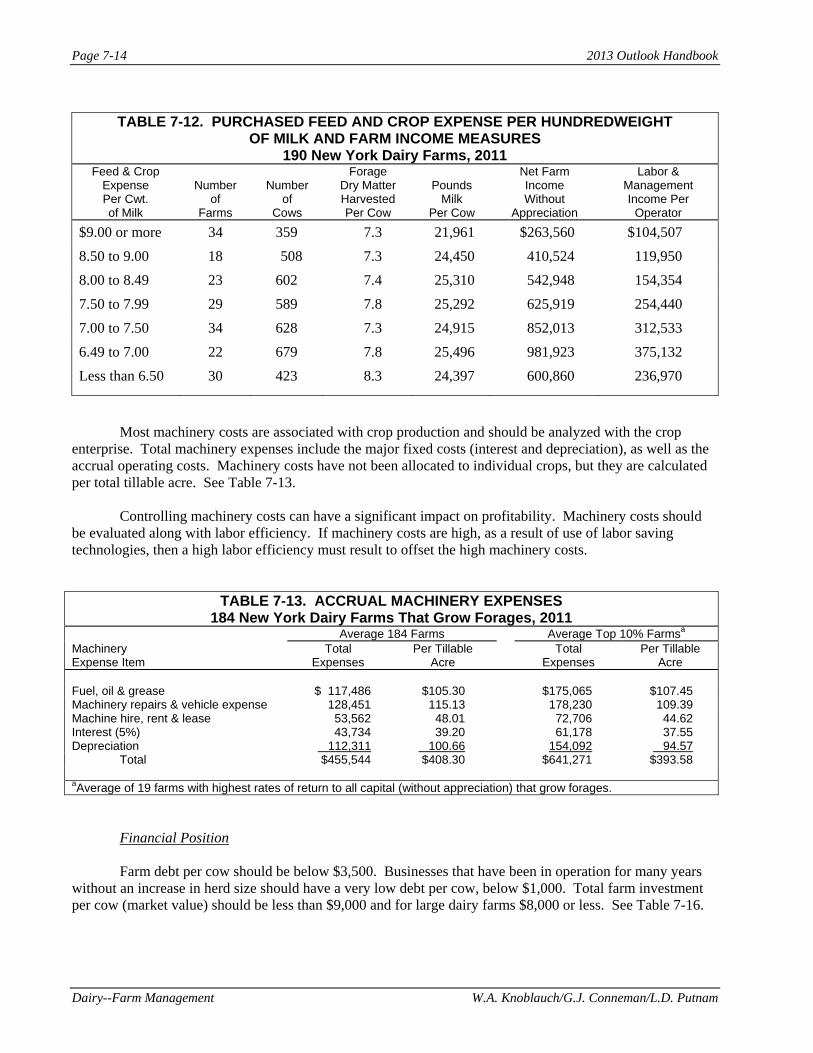
2013 Outlook Handbook
Dairy--Farm Management W.A. Knoblauch/G.J. Conneman/L.D. Putnam
Page 7-14
TABLE 7-12. PURCHASED FEED AND CROP EXPENSE PER HUNDREDWEIGHT
OF MILK AND FARM INCOME MEASURES 190 New York Dairy Farms, 2011
Feed & Crop Expense Per Cwt. of Milk
Number
of Farms
Number
of Cows
Forage Dry Matter Harvested Per Cow
Pounds
Milk Per Cow
Net Farm Income Without
Appreciation
Labor & Management Income Per
Operator
$9.00 or more 34 359 7.3 21,961 $263,560 $104,507
8.50 to 9.00 18 508 7.3 24,450 410,524 119,950
8.00 to 8.49 23 602 7.4 25,310 542,948 154,354
7.50 to 7.99 29 589 7.8 25,292 625,919 254,440
7.00 to 7.50 34 628 7.3 24,915 852,013 312,533
6.49 to 7.00 22 679 7.8 25,496 981,923 375,132
Less than 6.50 30 423 8.3 24,397 600,860 236,970
Most machinery costs are associated with crop production and should be analyzed with the crop enterprise. Total machinery expenses include the major fixed costs (interest and depreciation), as well as the accrual operating costs. Machinery costs have not been allocated to individual crops, but they are calculated per total tillable acre. See Table 7-13. Controlling machinery costs can have a significant impact on profitability. Machinery costs should be evaluated along with labor efficiency. If machinery costs are high, as a result of use of labor saving technologies, then a high labor efficiency must result to offset the high machinery costs.
TABLE 7-13. ACCRUAL MACHINERY EXPENSES 184 New York Dairy Farms That Grow Forages, 2011
Average 184 Farms Average Top 10% Farmsa Machinery Expense Item
Total Expenses
Per Tillable Acre
Total Expenses
Per Tillable Acre
Fuel, oil & grease $ 117,486 $105.30 $175,065 $107.45 Machinery repairs & vehicle expense 128,451 115.13 178,230 109.39 Machine hire, rent & lease 53,562 48.01 72,706 44.62 Interest (5%) 43,734 39.20 61,178 37.55 Depreciation 112,311 100.66 154,092 94.57 Total $455,544 $408.30 $641,271 $393.58 aAverage of 19 farms with highest rates of return to all capital (without appreciation) that grow forages.
Financial Position Farm debt per cow should be below $3,500. Businesses that have been in operation for many years without an increase in herd size should have a very low debt per cow, below $1,000. Total farm investment per cow (market value) should be less than $9,000 and for large dairy farms $8,000 or less. See Table 7-16.

2013 Outlook Handbook
W.A. Knoblauch/G.J. Conneman/L.D. Putnam Dairy--Farm Management
Page 7-15
Farm Business Charts For a complete analysis of the business, a farm business chart can be very useful. The Farm Business Chart is a tool which can be used in analyzing a business by drawing a line through the figure in each column which represents the current level of management performance. The figure at the top of each column is the average of the top 10 percent of the 190 farms for that factor. The other figures in each column are the average for the second 10 percent, third 10 percent, etc. Each column of the chart is independent of the others. The farms which are in the top 10 percent for one factor would not necessarily be the same farms which make up the 10 percent for any other factor. See Tables 7-14 and 7-15. The cost control factors are ranked from low to high, but the lowest cost is not necessarily the most profitable. In some cases, the “best” management position is somewhere near the middle or average. Many things affect the level of costs, and must be taken into account when analyzing the factors.
TABLE 7-14. FARM BUSINESS CHART FOR FARM MANAGEMENT COOPERATORS 190 New York Dairy Farms, 2011
Size of Business Rates of Production Labor Efficiency
Worker Equiv- alent
No. of
Cows
Pounds
Milk Sold
Pounds
Milk Sold Per Cow
Tons
Hay Crop DM/Acre
Tons Corn
Silage Per Acre
Cows Per
Worker
Pounds
Milk Sold Per Worker
37.4 1,706 43,858,755 27,706 5.3 23 63 1,458,922 22.9 1,021 26,336,021 26,440 4.4 20 51 1,243,329 17.6 785 20,082,453 25,674 3.9 18 48 1,167,110 14.1 612 14,432,284 24,907 3.6 18 45 1,088,025 10.6 466 11,020,599 24,206 3.4 17 42 1,010,627
7.0 325 7,344,654 23,151 3.1 16 40 925,116 4.7 174 3,679,214 21,982 2.8 15 37 793,037 3.1 108 2,120,345 20,278 2.3 14 33 667,413 2.3 69 1,296,787 17,715 2.1 13 28 550,182 1.6 45 726,923 12,283 1.6 10 21 343,454
Cost Control
Grain Bought
Per Cow
% Grain is of Milk
Receipts
Machinery Costs
Per Cow
Labor & Machinery
Costs Per Cow
Feed & Crop Expenses Per Cow
Feed & Crop Expenses Per
Cwt. Milk $651 18% $493 $1,152 $898 $5.24 1,014 23 651 1,413 1,300 6.42 1,136 26 716 1,533 1,473 6.94 1,258 27 779 1,625 1,617 7.24 1,384 28 843 1,691 1,739 7.55
1,475 29 901 1,759 1,827 7.82 1,564 31 960 1,842 1,936 8.19 1,653 32 1,038 1,933 2,030 8.61 1,731 34 1,126 2,102 2,150 9.24 1,947 38 1,384 2,606 2,388 10.66
The next section of the Farm Business Chart provides for comparative analysis of the value and costs of dairy production.

2013 Outlook Handbook
Dairy--Farm Management W.A. Knoblauch/G.J. Conneman/L.D. Putnam
Page 7-16
The profitability section shows the variation in farm income by decile and enables a dairy farmer to determine where he or she ranks by using several measures of farm profitability. Remember that each column is independently established and the farms making up the top decile in the first column will not necessarily be on the top of any other column. The dairy farmer who ranks at or near the top of most of these columns is in a very enviable position. TABLE 7-15. FARM BUSINESS CHART FOR FARM MANAGEMENT COOPERATORS
190 New York Dairy Farms, 2011 Milk
Receipts Per Cow
Milk Receipts Per Cwt.
Operating Cost Milk Production
Per Cow
Operating Cost Milk Production
Per Cwt.
Total Cost Milk Production Per Cow
Total Cost Milk Production Per Cwt.
$6,127 $23.60 $1,932 $12.19 $3,184 $16.71 5,705 22.51 2,646 13.62 3,969 17.95 5,520 22.08 3,015 14.29 4,328 18.65 5,369 21.81 3,355 14.98 4,506 19.22 5,188 21.63 3,601 15.53 4,650 19.75
4,959 21.41 3,740 16.05 4,757 20.34 4,719 21.21 3,881 16.62 4,910 21.30 4,381 21.00 4,083 17.35 5,104 22.92 3,837 20.75 4,353 17.88 5,317 25.38 2,658 20.24 4,711 19.90 5,728 31.41
Profitability
Net Farm Income Without Appreciation
Net Farm Income With Appreciation
Labor & Management Income
Total
Per Cow
Operations Ratio
Total
Per Cow
Per Farm
Per Operator
$2,341,294 $1,900 0.31 $2,707,050 $2,395 $1,794,884 $864,454
1,264,736 1,606 0.27 1,485,514 1,927 951,356 476,538 867,967 1,344 0.23 1,079,176 1,610 628,200 311,166 616,369 1,165 0.20 792,265 1,395 457,712 212,547 438,110 1,017 0.18 552,379 1,238 289,617 153,689
274,291 913 0.16 349,944 1,111 150,363 84,765 143,833 773 0.14 185,513 994 66,657 48,741 80,696 612 0.12 109,297 833 29,919 20,449 34,852 399 0.09 56,294 566 -10,042 -8,376
-10,917 -25 -0.01 15,314 222 -90,536 -56,785
The farm financial analysis chart, Table 7-16, is designed just like the farm business chart shown in Tables 7-14 and 7-15 and may be used to measure the financial health of the farm business.

2013 Outlook Handbook
W.A. Knoblauch/G.J. Conneman/L.D. Putnam Dairy--Farm Management
Page 7-17
TABLE 7-16. FINANCIAL ANALYSIS CHART 190 New York Dairy Farms, 2011
Liquidity/Repayment Planned
Debt Payments Per Cow
Available For Debt Service Per Cow
Cash Flow Coverage
Ratio
Debt
Coverage Ratio
Debt Payments as Percent
of Milk Sales
Debt Per Cow
Working Capital as % of Total Expenses
Current Ratio
$ 63 $1,607 10.52 13.41 3% $ 133 57% 48.32 283 1,339 3.30 4.56 5 1,137 41 6.16 419 1,157 2.47 3.36 7 1,841 31 3.96 485 989 1.96 2.79 9 2,316 26 3.17 575 867 1.64 2.34 10 2,787 21 2.54
642 750 1.45 1.96 11 3,167 17 2.01 703 641 1.23 1.61 13 3,635 13 1.74 799 558 1.02 1.30 15 4,210 10 1.43 932 444 0.88 0.83 17 4,916 4 1.05 1,446 86 0.24 0.08 25 6,691 -13 0.41
Solvency Operational Ratios Debt/Asset Ratio Operating Interest Depreciation
Leverage Percent Current & Long Expense Expense Expense Ratioa Equity Intermediate Term Ratio Ratio Ratio 0.01 99% 0.01 0.00 0.61 0.00 0.02 0.12 89 0.09 0.00 0.65 0.01 0.04 0.20 83 0.17 0.01 0.68 0.01 0.04 0.27 79 0.24 0.10 0.70 0.01 0.05 0.35 74 0.27 0.19 0.73 0.02 0.06
0.48 68 0.32 0.30 0.75 0.02 0.06 0.61 62 0.37 0.39 0.77 0.03 0.07 0.75 57 0.43 0.49 0.79 0.03 0.08 0.98 51 0.54 0.59 0.82 0.04 0.10 1.91 38 0.73 0.83 0.89 0.08 0.14
Efficiency (Capital) Profitability
Asset Turnover
(ratio)
Real Estate Investment Per Cow
Machinery Investment Per Cow
Total Farm Assets
Per Cow
Change in Net Worth
With Appreciation
Percent Rate of Return With Appreciation on:
Equity Investmentb
0.92 $1,960 $662 $6,389 $2,323,290 35% 23% 0.77 2,744 1,032 7,721 1,203,378 25 17 0.70 3,065 1,335 8,235 886,807 22 15 0.65 3,357 1,567 8,929 659,342 19 14 0.61 3,684 1,735 9,627 394,739 16 12
0.57 4,277 1,884 10,269 256,529 12 10 0.52 4,745 2,046 11,111 116,070 9 8 0.47 5,543 2,367 11,989 63,416 6 5 0.39 6,721 2,816 13,236 23,571 0 1 0.27 9,736 4,002 16,747 -6,842 -18 -4
aDollars of debt per dollar of equity, computed by dividing total liabilities by total equity. bReturn on all farm capital (no deduction for interest paid) divided by total farm assets.
2013 Outlook Handbook
Dairy--Farm Management W.A. Knoblauch/G.J. Conneman/L.D. Putnam
Page 7-18
Conclusion
The saying “You can’t manage what you can’t measure” is equally valid in dairy farm management as it is in an industrial or commercial business. Effective managers measure the most important factors for success in their business, compare the values with the performance of similar businesses and set annual goals for improvement. The most effective goals are SMART. That is, they are Specific, Measurable, Attainable, Rewarding and Timed. Annually setting goals and then measuring progress towards goals is an important component of management. Research has shown that goals that are written are much more likely to be achieved than are goals that are only verbalized or goals that are not shared. Evaluating a dairy farm business is not something to do once in a lifetime, but rather progress should be measured annually and new goals set for the following year. If a farm is not moving forward while other farms are, then the farm is moving backward relative to the industry. Performing an annual analysis and setting goals for the future is an excellent process to use in moving your business forward.

M.A. Smith and T.R. Maloney Labor-Intensive Agriculture
Chapter 8. Risk and Opportunity for Labor-Intensive
Agriculture in 2013 Marc A. Smith, Senior Extension Associate
Thomas R. Maloney, Senior Extension Associate
Introduction
Farm employers continue to be concerned about difficulties in hiring an adequate number of
productive, motivated and legal workers to perform the most labor-intensive agricultural production jobs.
The presence of unauthorized agricultural workers in New York and around the country creates uncertainty
and risks for farm managers attempting to complete farm operations in a timely manner to ensure product
quality and ultimately farm profitability. Anecdotal reports indicate that some New York farmers faced
tighter labor supplies this year as compared to the previous several years. Some reported fewer workers
available at peak harvest periods resulting in harvest delays. This was particularly true with the New York
apple crop. Several factors contributed to the shortage of workers. Cold spring temperatures led to a severe
decrease in the New York apple crop prompting many harvest workers to seek work in other states.
Immigration enforcement pressure also appears to have deterred workers from traveling to New York to seek
jobs in the fruit and vegetable industries. Immigration enforcement officials maintained a continuous
presence with an increased focus on the dairy industry in New York 2012. Farm employers using the H-2A
program occasionally report difficulties with the program including the rejection of worker applications and
problems with worker qualifications. Many New York farm employers continue to use the H-2A program
despite its high costs and administrative requirements because it is a way to reduce the risks associated with
not having a sufficient supply of legally authorized workers during critical work periods. Because of these
challenges, many New York farm employers are pessimistic regarding the farm labor outlook and report that
they are reluctant to expand farm operations when such a high level of labor supply uncertainty exists. In
addition, some farm owners report that they have shifted some of their fresh vegetable and fruit production to
highly mechanized row crop production. Although immigration was an important campaign topic, no
progress on immigration reform was expected during the 2012 Presidential election year. However, now that
a new Congressional session is set to start on January 1, 2013, farm employers are hopeful that progress can
be made on immigration reform including workable solutions for agriculture.
Important Immigration Issues 2012
In the absence of Federal immigration in 2012, several important labor issues including mandatory
E-Verify, the Executive Order DREAM Act, and the ongoing challenges with H-2A each received
considerable attention from agricultural leaders.
Mandatory E-Verify E-Verify is an internet based system that allows employers to check
information on the employees I-9 form against the databases from the U.S. Department of Homeland Security
and the Social Security Administration to confirm that the employee has legally entered the United States.
E-Verify is currently a voluntary program available to employers through the Department of Homeland
Security. In June 2011, a bill was introduced in the House Judiciary Committee that would make E-Verify
mandatory for most employers in all states. The proposed Legal Workforce Act (HR 2164) would repeal the
current I-9 system and gradually phase in mandatory participation in E-Verify. Opposition from agriculture
to the proposal was strong and immediate. Agricultural leaders insisted that the measure would cause serious
problems for agriculture if a large number of unauthorized workers were to exit farm employment.
Representative Lamar Smith, House Judiciary Committee Chairman and sponsor of the bill, tried to move the
legislation throughout 2011. Attempts were also made to modify the bill by adding solutions that would help

2013 Outlook Handbook
Labor-Intensive Agriculture M.A. Smith and T.R. Maloney
Page 8-2
agricultural employers. Congressman Smith continued to advocate for mandatory E-Verify into the 2012
Presidential election year with no success, diminishing the likelihood that the stand alone bill would be
successful in the House of Representatives. If introduced in the next Congress, it is unlikely that mandatory
E-Verify would move on its own, but it is very likely that it will be an important part of any comprehensive
immigration reform legislation. Agricultural leaders appear willing to support mandatory E-Verify legislation
as long as it is accompanied by a process for hiring an adequate supply of legally authorized agricultural
workers.
“Executive Order DREAM Act" In June 2012, President Obama issued an executive order intended
to halt the deportation of illegal immigrants who arrived in the United States as children. It is estimated that
at least 800,000 unauthorized immigrants fall into this category. The intent of the Executive Order is to
protect from enforcement actions young immigrants who are brought to this country as children, know only
this country as home, and lacked the intent to violate the law. It is intended to temporarily remove the threat
of immigration enforcement for young immigrants until a long-term legislative solution can be found. To be
eligible young immigrants must meet several criteria. They must have: entered the United States under the
age of 16; continuously resided in the United States for at least five years; have participated in the U.S.
education system or been honorably discharged from the Armed Forces; have not been convicted of a felony
offense and not be above the age of 30. In agriculture there appears to be a small number of workers and
children of agricultural workers who will benefit from this action while waiting for a legislative solution.
H-2A Challenges In the absence of immigration reform a number of agricultural employers
continue to rely heavily on the H-2A program to meet their labor needs. Despite its high costs and
bureaucratic challenges, some farmers continue to use the program to ensure that they will have the legal
workers they need on a timely basis. As immigration policy discussions move forward, it is likely that
recommendations from agriculture will include a major overhaul or replacement of the current H-2A system.
It is also important to note that immigrant workers are important to the dairy industry and there is no
opportunity for dairy farm employers to hire temporary workers under the H-2A system. It is expected that
this issue also will also be part of any H-2A and guestworker discussions in the year ahead.
Mexican Migration In April 2012, the PEW Hispanic Center released a report describing numerous
changes in the migration patterns from Mexico to the United States. Over the last four decades migration
from Mexico, (much of it illegal migration) increased rapidly. However in recent years it has come to a
standstill. There are a number of factors contributing to these changes. Increasing unemployment in the
United States and a week job market has meant fewer job opportunities for Mexicans in the United States
decreasing the incentive to migrate. At the same time enforcement at the U.S.- Mexican border has reduced
the number of border crossings while criminal activity and the number of deportations by the Department of
Homeland Security have increased. In addition, crime at the border has made illegal crossings far more
dangerous so many Mexicans are reluctant to make the attempt.
Conditions in Mexico are also likely to make a difference in the number of Mexicans migrating to the
United States in the years ahead. Mexican women are having significantly fewer children than they were a
few decades ago. In 1960, Mexico had a birth rate of 7.3 children per woman. In 2009, that figure dropped to
2.4, slightly higher than the U.S. rate of 2.0 children per woman. Looking ahead, there will be fewer Mexican
young people available to fill agricultural jobs than there have been in recent decades. At the same time the
Mexican economy is slowly improving. In the past two years the growth in the Mexican economy has been
stronger than in the United States. While median income is still a concern, the Mexican economy is in a
better position to create jobs than it was several years ago. All of these factors suggest that as U.S. employers
seek immigrant employees to fill labor-intensive jobs; those employees will increasingly come from countries
other than Mexico.

2013 Outlook Handbook
M.A. Smith and T.R. Maloney Labor-Intensive Agriculture
Page 8-3
The Political Economy of Agriculture and Immigration Reform
Even before voters went to the polls on November 6th, President Obama designated immigration
reform as a high priority for his second term; and after the results came in leaders of the Republican Party
appeared willing to consider meaningful changes to the status quo. Americans of Hispanic origin, by a
margin of 71%-27%, voted for the President, strengthening the administration’s resolve and prompting an
apparent change of heart by many reform opponents in Congress. For agriculture, this impending period of
action on federal policy will present both real opportunities and significant risks.
Countless, very diverse interest groups, from the National Council of Agricultural Employers to the
National Association of Evangelicals, the U.S. Chamber of Commerce and the League of United Latin
American Citizens, have profound stakes in the outcomes of any legislative process leading to immigration
reforms that are now decades overdue. Since the last meaningful reform of the nation’s immigration policies
in 1986, each of these groups has developed agendas that have taken on new importance now that the 2013
window seems to be open. These individual agendas for change emphasize different aspects of this complex
issue. The risks associated with a comprehensive approach to reform stem from conflicts among the priorities
championed by disparate groups that appear, at least on the surface, to share a common cause for change. If
such differences are not resolved, employers as well as advocates for immigrant rights risk wasting “the
moment” or producing policies and regulations that fail to repair the currently broken system or even make
the situation worse. Agriculture is only one voice in this highly charged pursuit of long unmet aspirations for
reform. A successful outcome will incorporate a functional, streamlined guest worker program and
provisions to deal with unauthorized immigrants already working and living in the United States, major
objectives for agricultural businesses, into a system that might also address high expectations for border
security, paths to citizenship, family reunification, the DREAM Act, opportunities for workers to move freely
within the U.S. labor market, changes in enforcement and detention and perhaps much more.
In the political swirl of what could be an unusually active legislative season, it is important to
remember the economic imperatives that drive urgent calls for immigration and labor policy reform from U.S.
farm employers. Labor costs make up an average of 48% of total expenses for fruit growers; 46% in nursery
operations; 35% for vegetable producers; and 14% for dairy farm businesses. The fact that New York’s dairy
industry (the state’s largest farm production sector) seeks year-round employees while fruit and vegetable
growers have met the challenges of securing a seasonal work force for decades complicates the political,
economic and management issues associated with federal labor policy reform. These sectors generate nearly
all of New York State’s $4.6 billion value of farm production. Occasional labor shortages and the almost
constant uncertainty that surrounds the availability of qualified workers push labor costs higher; as does
meeting the requirements associated with acquiring workers through the H-2A program. One Hudson Valley
fruit grower illustrates important aspects of the labor economics situation from his farm vantage point this
way:
“In apples, labor accounts for about 40% of our cost of production. And I continue to consider it our
largest business risk, since crop insurance does not cover a labor shortage. Bottom line? An acute labor
crunch cannot be overcome by H-2A alone and will cause some of our businesses to fail. Labor- intensive tree
crops (apples and stone fruit) have long- term, large capital investment and cannot be realigned into other
agricultural uses very quickly. In Eastern New York much of our terrain and soils are not even usable for
other crops. In my opinion, food production requiring significant labor will continue to move to other
countries where the labor is willing and able unless our federal government and the 2nd term President can
put politics aside and come to workable solutions.”
This is a critical economic issue for New York State agriculture.

2013 Outlook Handbook
Labor-Intensive Agriculture M.A. Smith and T.R. Maloney
Page 8-4
In the 113th
Congress
Shortly after the election, House Speaker John Boehner joined the President in singling out
comprehensive immigration reform as an achievable legislative goal for the administration and the new
Congress. After decades of Congressional inaction on federal immigration policy, positive, post-election
comments from House and Senate leaders appear to have opened the door for meaningful reform during the
next two years. Behind the sound bites, however, it will be essential for advocates for agricultural employers
and workers alike to understand who in Congress will be charged with moving reform legislation forward and
to participate actively and in concert to achieve well-defined goals as the political “sausage-making” process
unfolds.
In the House of Representatives, the Judiciary Committee and its Subcommittee on Immigration
Policy and Enforcement are responsible for action on immigration reform. Robert Goodlatte (R-VA) will take
over as chair of the Judiciary Committee; and Steve King (R-IA) will probably move into the chairmanship of
the immigration subcommittee. Both have been active, vocal opponents of less restrictive immigration laws
such as those proposed in the most recently failed comprehensive reform legislation, S. 3932/H.R.4321 in
2010; and DREAM Act provisions incorporated into President Obama’s “deferred action” policy announced
in June 2012. Speaker Boehner will need to exercise all of the leadership influence at his disposal if he is
serious about moving a comprehensive reform package through this committee to the House floor. In the
lame duck House, current Judiciary chair Lamar Smith (R-TX) has introduced a revised version of an earlier
“STEM” bill, designed to increase the number of visas available to overseas students who have earned
advanced degrees in science and technology at U.S. universities. Some regard this as a signal that
Republicans are prepared to move ahead on additional reforms in the new session.
The U.S. Senate is likely to take the lead in moving immigration bills forward and would develop
proposed immigration reform legislation in the Senate Judiciary Committee, chaired by Patrick Leahy (D-VT)
and its Subcommittee on Immigration, Refugees, and Border Security, led by Charles Schumer (D-NY). The
subcommittee is populated by senior senators who are leaders in their respective political parties and of the
Senate itself, including Democrats Richard Durbin (D-IL) and Diane Feinstein (D-CA) and Republicans
Charles Grassley (R-IA), Jon Cornyn (R-TX), and Orrin Hatch (R-UT). As in the House, a test of Republican
intentions to move toward broad immigration reform will be considered during the Senate’s lame duck
session. Departing Senators Kay Bailey Hutchinson (R-TX) and Jon Kyl (R-AZ) have submitted a
Republican version of the DREAM Act bill, which failed to come up for a vote in December 2011. Rising
Republican Party star, Senator Marco Rubio (R-FL) has also signaled his intentions to play a lead role in the
coming debate.
In the Obama Administration
In September, Jorge Ramos and Maria Elena Salinas, the well-respected anchors of the Spanish
language program Univision Noticiero, called President Obama to task in front of a nationwide audience of
Latino voters on his unfulfilled campaign promise to introduce and work with Congress to pass
comprehensive immigration reform legislation early in his first term. In response, Mr. Obama said, "My
biggest failure so far is we haven’t gotten comprehensive immigration reform done, so we’re going to be
continuing to work on that. It’s not for lack of trying or desire, and I’m confident we’re going to accomplish
that." The decisive Hispanic vote for the President less than two months later heightened expectations for the
new term and appears to have moved the issue to a place just behind “fiscal cliff” resolution for action early
in 2013.
As noted above, achieving comprehensive immigration reform will require fitting many complicated
moving parts (policy, regulation, enforcement) together into a functional national system. Key officials in

2013 Outlook Handbook
M.A. Smith and T.R. Maloney Labor-Intensive Agriculture
Page 8-5
the administration will be called upon to take on this difficult task with their Congressional counterparts. For
example, Secretary of Education Arne Duncan, who apparently will stay on for the second term, was the
President’s point person in the failed 2011 attempt to move the DREAM Act through the last lame duck
Congress. Secretary of Labor, Hilda Solis wants to continue in the new term. Her department administers
H-2A and other current programs and regulations that could be targeted for reform in 2013. There is
speculation that Department of Homeland Security Secretary, Janet Napolitano, wants to be Attorney General,
but if Eric Holder continues for another year, she will play a major role in determining the enforcement
implications of any immigration law reforms. The length of Secretary of Agriculture Tom Vilsack’s tenure
seems uncertain, but whoever leads that department in the new term will have an important voice in how any
new approaches to agricultural labor policy might evolve. The political discussion has already moved USDA
into a more important position given the desire of many agricultural advocates to move administration of
existing and proposed regulatory programs and regulations to that department.
On the Farm
While leaders of farm organizations such as the American Farm Bureau Federation and the
Agriculture Council for Immigration Reform have been working overtime to build agricultural sector unity in
anticipation of an apparent moment of political opportunity to reform a broken system, many New York
growers remain highly skeptical of Washington’s ability to capitalize on that moment. One prominent
vegetable grower in the Finger Lakes puts it this way, “I have no faith that the government will fix the
problem or if they try to, that it will be a workable system… I am looking to solve our problem by making
changes in our business, not expecting to fix a system to make it work for the long term.” Moreover, on-farm
decisions during the long period of governmental paralysis on this issue have started to reflect such
pessimism. A Western New York fruit grower described one such decision, “Corn for grain and soybeans are
looking less risky than planting new orchards. I have no faith that Congress will do anything but continue the
posturing they have been doing with no action. Our plan for the next few years is to plant one acre of orchard
for every two that we take out and grow more grains.”
In addition to considering changes in crop mixes to move away from labor-intensive production,
farmers have taken a variety of other steps to manage labor uncertainty in their businesses. Many of these
were described in the 2012 New York Economic Handbook. Given projections of curtailed migration from
Mexico to the United States, it will be critical that farmers access alternative labor sources aggressively and
effectively, regardless of progress on policy reform in 2013.
Successful “hire local” strategies, for example, are characterized by recruitment via social media and
other non-traditional means, creative compensation packages, flexibly-designed work schedules, a
continuous, intensive focus on training, significant interaction among managers and employees, and a
willingness by employers to hire workers with relatively little agricultural experience, but who are eager to
learn and commit to the success of the business.
In Western New York fruit growers and dairy farmers have worked closely with church support
groups and regional transit authorities to improve opportunities for refugee employment in agriculture.
Potential refugee workers have valid visas, valuable agricultural skills and a strong work ethic to offer.
Nearly all refugees, however, have settled in cities, making the high cost of transportation a limiting factor in
efforts to match employees with promising farm jobs in relatively isolated rural areas. Farm operations close
to the “end of the line” for regional bus routes have successfully employed workers from this labor pool; and
collaborative pilot programs to solve the transportation problem for employers farther from the city are
underway.
Given the post-election “open door” for immigration reform and all its possible ramifications for farm
employment, it will be more important than ever for New York State’s labor-intensive agricultural businesses
2013 Outlook Handbook
Labor-Intensive Agriculture M.A. Smith and T.R. Maloney
Page 8-6
to participate actively and constructively in the political process during 2013. New York Farm Bureau
(NYFB) has already moved aggressively with the American Farm Bureau Federation (AFBF) to start crafting
a policy framework that will work for the state’s diverse agricultural employers. Julie Suarez, Public Policy
Director for NYFB, recently reported on her participation in an AFBF immigration task force consisting of
farm leaders from California, Arizona, New York, North Carolina, Washington, Louisiana, Michigan, Florida,
Ohio, Pennsylvania, and New Jersey. This important group made policy recommendations for reform that
would bridge difficult interregional differences and set the stage for a united grassroots agricultural campaign
for positive immigration reform provisions in federal law and regulatory practice. These recommendations
were incorporated into AFBF’s Agricultural Labor-Immigration Reform policy statement, issued in October
2012. The ultimate goal of this effort is the introduction of agricultural worker program legislation that will
resolve existing needs for full-time workers and provide a means to replenish the farm work force in the
future.
The Way Forward
Bringing Farm Bureau leaders from states with very different political priorities together behind
consensus labor policy proposals represents a major political step forward for labor-intensive agriculture.
Now that agriculture has found its one voice, farm business leaders will gain additional leverage from
building constructive, perhaps unusual alliances with other very influential groups engaged in their own long
running efforts to repair the nation’s immigration system.
Key considerations for New York State producers as the debate unfolds include:
1. Maintaining strong lines of communication with Senator Schumer’s office due to his leadership
role in this matter, and other members of the New York congressional delegation.
2. Understanding the points on which compromise with various advocacy groups could be necessary
and which principles must be defended. For example, the issue of “portability”, or the
opportunities workers with visas will have to move from job to job throughout the labor market,
has not been resolved.
3. Maintaining strong lines of communication with officials in important executive branch
departments.
4. Emphasizing areas where Hispanic American and worker advocate priorities coincide with those
of agricultural employers.
5. Maintaining and reinforcing a unified agricultural position on immigration reform.
The New York Agricultural Outlook for 2013
New York farm managers who hire immigrant agricultural workers continue to urge Congressional
leaders to address immigration reform. Enforcement efforts at both the employer and the employee level
create uncertainty for many farm operations. A legislative solution is viewed by many as the most
constructive way forward. The 2012 Presidential and Congressional elections have created some optimism
that 2013 could bring immigration policy changes allowing unauthorized immigrants legal authorization to
work in the United States and addressing the need for a workable guest worker program in agriculture.
We anticipate the following agricultural labor conditions as we look ahead to 2013.
1) Enforcement - In the absence of legislative solutions to the immigration challenges facing
agriculture, the risks and uncertainties related to immigration enforcement at the employer level
and the worker level will continue. Detentions and deportations of immigrants working on New
York farms are ongoing. Enforcement at the employer level in the form of I-9 audits has

2013 Outlook Handbook
M.A. Smith and T.R. Maloney Labor-Intensive Agriculture
Page 8-7
increased in recent years. The audits are time-consuming for farm managers and bring with them
the potential that employment of some immigrants will be terminated if they are determined to be
unauthorized. This situation continues to create staffing problems for farm managers attempting
to plan for their workforce needs, particularly when harvesting perishable crops.
2) Continued pressure for immigration reform - The Presidential and Congressional elections
created an opportunity to discuss immigration reform and Hispanic voters had a major influence
on the election. President Obama and Congressional leaders appear willing to recommit to
legislative solutions to address the country's immigration problems. One of the greatest
challenges facing agricultural employers is the ongoing presence of unauthorized immigrant
workers. Farm employers are likely to support proposals that will allow unauthorized immigrants
the opportunity to stay in the United States to work. Farm employers in labor-intensive
agriculture rely heavily on the immigrant workforce and feel that legal status for immigrant
workers will help ensure the future viability of their businesses. In recent months, agricultural
organizations that represent agricultural employers have worked hard to unify around a set of
policies that all parties can support and to advocate for those policies in the next Congress.
3) Continued pressure to improve the H-2A program - Many of New York's fruit and vegetable
growers depend heavily on the H-2A program for a reliable source of legal immigrant workers.
Throughout its history, farm employers have highlighted some of the difficulties in using the
program. Wage rates are high, transportation and housing must be provided by the employer and
there is considerable paperwork required on the part of the employer. In recent years farm
managers have been concerned about work order rejections and delays in workers arriving to the
farm. Many farm employers who use the program suggest that the program should either be
substantially overhauled or replaced by a new program that will be less expensive and easier for
employers to use. It is likely that upcoming discussions of immigration reform for agriculture
will include proposals for a more effective guestworker program.
4) Employers will weigh labor options - In the year ahead it is very likely that farm employers will
continue to make careful decisions about the meeting their labor needs. They will continue to
look for alternatives to unauthorized workers. Some have already looked at the possibility of
using refugees or foreign-born workers entering the United States on J-1 training visas. Some
farm managers have renewed efforts to attract and retain local employees. Others have switched
from labor-intensive fruits and vegetables to more mechanized crops. Continued interest in
mechanization to replace some labor is likely. Many farm employers would prefer to hire
immigrant workers but are concerned about the possibility that they are unauthorized so they
continue to look for alternatives.

Notes

B.J. Rickard Fruits and Vegetables
Chapter 9. Fruits and Vegetables Bradley J. Rickard, Assistant Professor
Charles H. Dyson School of Applied Economics and Management
Specialty crops are an important component of New York State’s agricultural economy. In 2011 the
total farm value of all agricultural products produced in New York was approximately $5.26 billion, which
has increased from the average total farm value over the period between 2006 and 2010. In 2011, fruit and
vegetable crops accounted for nearly 13% of the total value of agricultural production in New York State.
Fruits and vegetables were planted on 232 thousand acres in New York State in 2010 and this represents only
6.3% of total harvested cropland. Therefore, the value generated from fruits and vegetables is nearly three
times the value generated from other crops on a per acre basis.
Horticultural commodities are an important component of agriculture in New York State and we
continue to see a significant quantity of fruits and vegetables produced in the State, and marketed to
consumers through various channels. New York State is a top-producing state of apples, tart cherries, pears,
grapes, cabbage, cauliflower, onions, pumpkins, snap beans, squash, and sweet corn. Apples and grapes are
the two highest revenue fruit crops in New York while cabbage, sweet corn, snap beans, squash, and onions
have been the five highest revenue vegetable crops in recent years; the value of production for each of these
crops exceeded $30 million in 2011.
Below I divide fruits and vegetables into two categories and take a closer look at market conditions in
each category. I examine production patterns, and provide an outlook, for fruit and berries, and vegetables
(fresh and processing) in New York State. In each case I review production and price data between 2009 and
2012, give an economic outlook on expected market conditions in 2013, and also provide some thoughts on
the long term marketing and policy issues for horticultural crops produced in New York State.
9.1 Fruit and Berry Situation and Outlook
Market conditions for major fruit crops in New York State were, overall, slightly more favorable in
2011 compared to 2010. Prices for the two major fruit crops in New York State, apples and grapes, were
higher in 2011 compared to 2010, and this is a key driver of the higher total values for these fruit crops in
2011. Crop values for several other fruit crops were also higher in 2011 relative to 2010; although production
was down for some crops, prices were up for most and the total value of these crops increased. In what
follows, I take a closer look at domestic prices and production values, consumption patterns, and international
market conditions for major fruit crops in 2011. Similar to last year, market conditions for grapes are
examined separately in Chapter 10. Overall, the total value of fruit (including grapes) in New York in 2011
was $351 million, up 9% from the value in 2010, but less than the peak values observed in 2007 and 2008.
Table 9-1 shows that 610 thousand tons of apples were produced in New York State in 2011, and that
this crop was valued at $251 million. The overall value of the 2011 crop was up relative to the 2010 crop; the
value of the fresh crop was up and the value of the processing crop was down in 2011 compared to 2010.
Table 9-1 also indicates that the average price of New York State apples increased in 2011 compared to 2010;
the price of apples increased in the fresh market but fell slightly in the processing market. The average price
for New York apples used in processing market was $196 per ton in 2011, and although this is lower than the
prices in 2007 and 2008, it remains much higher than the seven-year average price observed between 2005
and 2011.

Page 9-2 2013 Outlook Handbook
Fruits and Vegetables B.J. Rickard
Once the official data from 2012 are released, I expect to see statistics that show a significant
decrease in apple production compared to 2011 and other recent years. Early evidence from the USDA Fruit
and Tree Nuts Outlook shows that U.S. apple production will be 8.1 billion pounds, which is down 14% from
2011 and the lowest crop in over two decades. The reduced crop was largely due to weather problems. In the
eastern states there were spring freezes that substantially reduced the number of buds, and in western states
there was a late spring hailstorm that affected production in some apple-growing regions. Overall, it appears
that production in western states is up slightly compared to 2011, but that eastern production is down by more
than 30% compared to 2011. In turn, we also expect to see a substantial increase in apple prices in 2012
compared to 2011, and we will likely see the per-capita consumption rate for apples fall below 15 pounds in
2012/2013. USDA-NASS reports indicate that apple prices were $0.529 per pound in August 2012, and this
is the second highest August price since 1985.
Relative to other states, New York continued to be a major national producer of apples in 2011. As
shown in Table 9-2, the value of U.S. apple production in 2011 was $2,750 million based on production of
9,500 million pounds and an average price of $0.292 per pound. Washington State typically produces
approximately 55 to 60% of the U.S. apple crop, but in 2012 Washington State is expected to produce about
70% of the national crop given the weather problems experienced in eastern states. In New York State,
production is forecast to be 590 million pounds in 2012 which is down 52% from 2011. This decrease is due
largely to the early spring frosts in 2012; it is also due to the hot and dry weather experienced during the
summer months which influenced fruit size and development.
In addition to apples, New York State is also a top producer of several other tree fruit and berry crops.
Table 9-1 shows that pear and peach production increased in 2011 versus 2010, while (tart and sweet) cherry
production decreased in 2011. Crop values also increased for peaches and pears but fell for sweet and tart
cherries in 2011. In 2011 New York State produced approximately $3.5 million in cherries ($1.4 million was
tart cherries and $2.1 was sweet cherries), $8.4 million in peaches, and $7.0 million in pears. Although not
shown in Table 9-1, berry production (including strawberries, blueberries, and red raspberries) was up in 2011
versus 2010, and the total value of berries produced in New York State increased by approximately $1.5
million in 2011 compared to 2010. The USDA Fruit and Tree Nuts Outlook reports an 8% decrease in pear
production in 2012 (down to 1.7 billion pounds), an 11% increase in sweet cherry production (up to 764
million pounds), and a substantial decline in tart cherry production (decreasing to 78 million pounds in 2012).
The tart cherry crop was nearly destroyed in Michigan in 2012 due to spring freezes, and Michigan is a major
producer of tart cherries in normal production years.
TABLE 9-1. COMMERCIAL NONCITRUS AND NONGRAPE FRUIT PRODUCTION
AND PRICES IN NEW YORK STATE
Production Prices
2009 2010 2011
2009 2010 2011
------ Thousand tons ------ ------ Dollars per ton ------
Apples 680 630 610 308 360 416
Fresh 338 300 283 450 526 666
Processed 342 330 322 166 209 196
Tart Cherries 5.1 3.9 3.0 486 348 484
Pears 9.9 8.3 12.1 490 519 600
Peaches 6.5 5.9 6.8 845 1200 1240
Sweet Cherries 1.2 1.0 0.7 2,440 2,820 3,140
Sources: New York Agricultural Statistics, 2012.

2013 Outlook Handbook Page 9-3
B.J. Rickard Fruits and Vegetables
Table 9-2 highlights the values of tree fruit crops in New York between 2009 and 2011; I also show
the total value of these crops nationally in 2009, 2010, and 2011. The information in Table 9-2 highlights that
New York apples and tart cherries are important nationally, pears and peaches are important for New York
State but have less of an impact on those markets nationally, and sweet cherries are a relatively small industry
in New York State. The value of the U.S. apple crop increased in 2011 relative to 2010, but will be smaller in
2012. The total value of peaches and cherries increased nationally in 2011, but the value of pears decreased
nationally in 2011. The smaller changes in values for peaches and cherries in New York State are likely due
to the regional marketing of these products that is more typical in the Northeast.
In addition to the differences in production and intra-national trade within the United States,
international trade continues to be important in fresh and processed fruit markets. Imports of fresh apples in
the United States reached a high of 472 million pounds in 2003/04 but have fallen recently; the United States
imported 381 million pounds of fresh apples in 2011/12 and is expected to import approximately 371 million
pounds in 2012/13. Imports of processed apple products have been steadily increasing in recent years, and
now the United States imports more apple juice that what it produces; approximately 80% of all apple juice
imports come from China. Exports of fresh apples from the United States have been relatively steady since
the mid-1990s, hovering around 1,700 million pounds per year. U.S. exports exceeded 1,800 million pounds
in 2010/11 and 2011/12, and are expected to be approximately 1,700 million pounds in 2012/13. Imports of
processed apple products have grown over the past fifteen years yet the value of each imported unit has fallen
over this time, and this will continue to present challenges to U.S. processors of apple products.
TABLE 9-2. VALUE OF NONCITRUS AND NONGRAPE FRUITS IN
NEW YORK STATE AND THE UNITED STATES
New York State United States
2009 2010 2011
2009 2010 2011
------ Million dollars ------
Apples 208.9 226.8 251.5 2,290.4 2,220.8 2,750.6
Fresh 151.9 157.8 188.1 - - -
Processed 56.9 68.9 63.2 - - -
Tart Cherries 2.5 1.4 1.4 63.2 40.5 69.5
Pears 4.9 4.3 7.0 355.2 381.7 372.3
Peaches 5.4 7.1 8.4 593.7 614.9 854.6
Sweet Cherries 2.3 2.8 2.1 505.9 721.2 867.8
Total 224.0 242.4 270.4 3,808.4 3,979.1 4,914.8
Sources: New York Agricultural Statistics, 2012; USDA Agricultural Statistics, 2011.
It is widely expected that there will be large crops of perennial fruits in eastern states in 2013 given
the reduced crop size in 2012. Perennial fruit trees are able to store unused starches in low production years
and carry them into the subsequent production cycle (in some capacity). If these crops are not properly
managed, there are indications that we could see a record apple crop in New York State and Michigan in
2013, and this will place downward pressure on apple prices for crops harvested in 2013 and for fruit stored
into 2014. Such downward pressure on apple prices would be compounded if Washington State continues to
increase production. During 2012 there was some discussion that Washington State’s apple production would
be below average, but it ended up being about 5% higher than average. This is due, in part, to the increased
plantings coming into production in Washington State. A record crop in eastern states coupled with a normal
or expanded crop in western states could have a significant effect on producer prices in 2013 and 2014.

Page 9-4 2013 Outlook Handbook
Fruits and Vegetables B.J. Rickard
U.S. consumption patterns for fresh, frozen, and canned fruit products between 2002 and 2007 were
examined in earlier editions of the Agricultural Outlook Handbook. Overall, we saw that per capita
consumption rates for most fresh and processed fruits had been relatively stable over this time. Consumption
rates had been very stable for frozen fruit products and showed a slight decline for many canned products.
The per capita apple consumption rates in the United States have been relatively stable between 2002 and
2007. They have also been below per capita consumption rates for bananas, and this is a pattern that reflects a
larger trend over the last two decades. We reproduce Table 9-3 from last year’s Agricultural Outlook
Handbook to reinforce trends in fresh fruit consumption patterns in the United States, and elsewhere. Fresh
fruit consumption (given in pounds per person) is provided in five different time periods between 1991 and
2009 in up to 12 countries. Apple consumption in the United States has remained in the range of 18 pounds
per person per year over this time period, yet it is expected to fall below 15 pounds per capita in 2012/13.
Trends in other countries are surprisingly different. In Canada per capita consumption of apples has been
closer to 26 pounds per person. The per capita consumption rate in many western European countries has
exceeded 30 or 40 pounds per person per year. Of the countries listed in Table 9-3, only Japan has a lower
per capita consumption rate of apples than the United States. This information indicates that apple marketers
need to develop very strategic plans to reach new consumers or expand apple sales to existing consumers.
TABLE 9-3. CONSUMPTION PATTERNS FOR SELECTED FRESH FRUITS
IN VARIOUS COUNTRIES
Consumption
1991-93 2001-03 2004-06 2007-09 2009
------ pounds per capita -------
Apples
United States 18.92 15.84 18.04 17.82 18.04
United Kingdom 24.64 20.46 22 22.22 22.66
Japan 12.32 12.76 11.22 12.54 12.76
Canada 26.4 25.08 29.48 28.6 28.82
Germany 52.36 40.26 41.8 42.9 42.9
France 30.8 35.64 35.64 33.22 33.88
Spain 38.94 41.14 33.88 30.36 27.94
Italy 46.64 44 37.84 37.84 38.94
New Zealand 32.34 35.64 29.92 29.04 28.82
China 11.88 28.38 29.04 36.3 43.34
Japan 12.32 12.76 11.22 12.54 12.76
Turkey 71.06 72.6 64.68 69.96 69.52
Bananas
United States 24.42 28.38 25.08 25.08 -
United Kingdom 14.3 24.42 25.74 26.4 -
Japan 15.4 14.52 16.28 17.6 -
Oranges
United States 12.32 8.36 11.88 11.88 -
United Kingdom 6.38 7.26 6.82 6.16 -
Japan 15.84 15.18 14.08 13.2 -
Source: World Apple Review, Belrose Inc., 2010.

2013 Outlook Handbook Page 9-5
B.J. Rickard Fruits and Vegetables
9.2 Fruit Outlook: Marketing and Policy Issues
Several economic and marketing issues that have been important to producers and packers of fruit
crops in New York State will continue to be key marketing concerns over the next two to five years.
Important and on-going issues include food safety concerns, labor availability, crop insurance rates,
promotion activities, and competition with foreign suppliers. Of the issues listed here, fruit producers in New
York State and elsewhere have indicated that labor availability remains as their top concern. This was also a
priority topic in the election cycle in 2012 and there are indications that Congress will look at new solutions
to this issue that is of paramount interest to fruit growers.
Farmers managing labor intensive specialty crop operations must cope with major risk and
uncertainty associated with the perennial challenges of hiring a legally authorized and reliable workforce in an
exceptionally challenging, seemingly intransigent immigration policy, regulatory and enforcement
environment. Aside from supporting continuing, yet so far fruitless political initiatives to reform current
federal policy, farmers have experimented with and adopted a variety of practices to manage such labor
risk. To date, only anecdotal evidence has informed our understanding of the effectiveness of these
alternative human resource management practices. Similarly, over the past decade Congress has entertained,
yet failed to pass a range of immigration policy proposals affecting agriculture, from targeted changes such as
the AgJobs bill to comprehensive reform legislation.
A 2009 Cornell study by Tom Maloney and Nelson Bills reports that there are approximately 11,200
Spanish-speaking immigrants performing labor-intensive jobs on New York State’s fruit and vegetable farms.
While projections vary, it is also estimated that 50% to 80% of immigrants working in U.S. agriculture are not
legally authorized, leaving them and the farm owners they work for vulnerable to a range of enforcement
actions. Farm workers face the possibility of detention and deportation. Farm owners face the possibility of
workforce disruptions during harvest and other critical work periods, as well as the possibility of fines and
other penalties. Practical alternatives to the unauthorized workforce must be found if labor-intensive
agriculture is to be viable in the future; and this is especially true in specialty crop markets.
New research at Cornell University aims to assess various labor options for specialty crop producers
to shed some new light on the relative costs of alternative ways to source and manage farm labor. We also
will conduct an analysis to evaluate how potential changes in labor policy might impact labor availability and
labor costs, and how any such changes might affect the competitiveness of specialty crop producers in New
York State. Labor represents the single largest cost for most producers of specialty crops, notably for
producers of fresh fruits and vegetables. Current levels of uncertainty about labor availability greatly add to
these costs. Anecdotal evidence also indicates that uncertainty concerning the future of labor availability
negatively affects investment among specialty crop producers, and this uncertainty could affect acreage
planted to labor intensive crops and the long-term sustainability of the specialty crop industry.
First, we intend to identify and describe the various strategies and practices followed by specialty
crop producers to secure and manage a reliable supply of qualified workers in recent years. Such practices
range from trying various approaches to participation in the federal H-2A program, to seeking out new
sources of labor, to experiments with mechanization and changes in planting strategies. We know growers
employ different strategies, but this information is not well documented, and the economic results of various
approaches are not known. In addition, different approaches may be used in different geographic regions and
by different types of specialty crop producers for specific reasons.
Second, we will examine how proposed changes in labor policy, particularly in the H-2A guest-
worker program, might affect labor availability and markets for specialty crop producers in New York State.
These policy findings, in conjunction with knowledge generated in the human resource management
component of the project will constitute a valuable package of information with which growers can improve

Page 9-6 2013 Outlook Handbook
Fruits and Vegetables B.J. Rickard
decisions about the adoption of the various labor management strategies. Although other researchers have
investigated the potential impact of greater agriculture labor supply in the United States, previous work has
not fully addressed labor market conditions in New York State.
9.3 Vegetable Situation
Total land planted to vegetables in New York State decreased from 128,500 acres in 2010 to 91,300
acres in 2011; planted and harvested acres of both fresh and processing vegetables were down in 2011, yet the
decrease in processing vegetable acreage was much more significant. Acreage used to produce processing
vegetables fell below half of the average level observed in recent years. The value of New York vegetable
production (including principal vegetables for fresh and processing markets but not including potatoes and
dry beans) decreased from $409 million in 2010 to $356 million in 2011; the value of fresh vegetables
decreased by about $50 million in 2011 compared to 2010. In 2010 fresh market vegetables contributed $329
million to the total (down from $374 million in 2010) while processed market vegetables contributed only $27
million in 2011 (which was down from $48 million in 2010).
The large decrease in planted acreage of processing vegetables in 2011 was due, in part, to record
rainfalls in the spring. However, the long-term decline in production in New York State is also due to
changing conditions in the structure of the industry. Across the United States, the production of processing
snap beans and green peas has decreased substantially between 2000 and 2011. Statistics indicate that there
has been a general decline in the production of these two processing vegetables nationwide and the green pea
industry has experienced more drastic changes in production than the snap bean industry. Wisconsin has been
the largest producer of snap beans nationally, followed by Oregon, New York and Minnesota. Minnesota
dominates national pea production followed by Washington, Wisconsin, New York, and Oregon. As one of
the top five producing states, New York plays an important role in supplying national markets for green peas
and snap beans. The latest data (2010 for snap beans and 2006 for green peas) show that New York State
accounts for about 10% of total national production. In recent years, we have seen dramatic declines in
planted acreage of green peas and downward trends in acres planted to other key processing vegetables grown
for freezing and canning. This is a critical concern for New York State farmers and is somewhat of an
enigma, given the fact that geographically the production areas are relatively close to big cities such as New
York City and Boston. A number of factors have combined to influence planting decisions and outcomes,
including historically high corn and soybean prices, a 48% decline in per capita use of canned and frozen
green peas since 1971, persistent production yield challenges for New York snap bean growers, increasing
concentration in the processing industry, and inventory decisions, especially for frozen vegetables, made by
New York processing firms during the past four years.
Preliminary market conditions reported in the September 2012 edition of the USDA Vegetables and
Melons Outlook suggest that prices for most fresh vegetables will be down slightly in 2012 compared to
levels observed in 2011. Even though we saw a hot and dry growing year in 2012, the volume of most
vegetable crops is higher than it was in 2011. The same Outlook report shows that total production of
processing vegetables is up in 2012, but still remains lower than the recent ten-year average observed in the
United States. Second quarter producer prices for fresh vegetables were 6.2% lower in 2012 relative to 2011;
some fell by nearly 40% over this time period. One notable exception was onion prices, which increased by
approximately 25% between the second quarter in 2011 and the second quarter in 2012. Consumer prices for
fresh vegetables were also lower in 2012 relative to 2011, but these have begun to rise during the fourth
quarter in 2012. A recent study by the USDA reports that the (loss-adjusted) per capita consumption of
vegetables increased by 17% between 1970 and 2010. Relative to 2011, exports of fresh vegetables were up
in 2012 by 3%, and imports were also up by 5%. U.S. exports of broccoli were up 31% in 2012 relative to
2011. Much of the change in export activity occurred with expansion into Chinese and Mexican markets.
Key export markets for vegetables continue to be Canada, Mexico, Japan, Taiwan, the United Kingdom, and
China.

2013 Outlook Handbook Page 9-7
B.J. Rickard Fruits and Vegetables
New York State continues to be a significant producer of onions, cabbage, and sweet corn; for each of
these commodities, New York State has often produced crops that have a value of $50 million or more. Total
crop values for some of these commodities fell below $50 million in 2011, but many (including onions,
squash, cabbage, snap beans, and sweet corn) had crop values that exceeded $30 million in 2011. Historically
New York State has produced a snap bean crop that had a value exceeding $50 million, but the snap bean crop
in has fallen short of this mark in recent years. In the tables and discussion that follow, we focus on recent
economic conditions, and provide some outlook, for nine fresh vegetable products and four processed
vegetable products that are important markets in New York. Table 9-4 shows production patterns for key
vegetables in New York State between 2009 and 2011. Data describing trends in fresh vegetable markets are
shown at the top of Table 9-4 and trends for processing vegetables are shown on the bottom portion of Table
9-4. Much of the most recent information for processing vegetables is not available from New York State
Department of Agriculture and Markets due to the small number of producers involved, budget constraints
facing the National Agricultural Statistics Service, and the proprietary nature of the data.
TABLE 9-4. COMMERCIAL VEGETABLE PRODUCTION AND PRICES IN
NEW YORK STATE
Production Price
2009 2010
2011
2009 2010
2011
Fresh ------ Thousand cwt ------ ------ Dollars per cwt ------
Sweet corn 2,150 2,736 1,862 27.10 26.00 28.80
Cabbage 3,496 4,343 4,708 17.00 18.70 20.00
Onions 4,275 3,087 1,891 18.60 19.70 20.80
Snap beans 268 469 323 88.00 83.60 96.10
Cucumbers 384 476 464 41.80 38.80 40.00
Tomatoes 350 392 432 93.50 72.70 84.80
Pumpkins 750 1,462 693 29.00 24.00 34.10
Squash 540 897 836 42.60 41.00 51.30
Cauliflower 52 67 49 45.50 51.00 49.00
Processing a
------ Thousand tons ------ ------ Dollars per cwt ------
Sweet corn - - - - - -
Snap beans 55.7 86.5 50.9 267.00 250.00 298.00
Green peas - - - - - -
Cabbage - - - - - -
Source: New York Agricultural Statistics, 2012.
a Much of these data are not published to avoid disclosure of individual operations.
Production of nearly all of the major fresh vegetable products in New York State was down in 2011
relative to 2010. Onions, in particular, are the one crop listed in Table 9-4 that showed a substantial decrease
in production in 2011 compared to 2010. Lower production levels led to higher prices for nearly all of the
fresh and processed vegetables listed in Table 9-4. Because of the downward trends in production and the
upward trends in prices in Tables 9-4, changes in the total values for the specified vegetable products were
mixed (see Table 9-5). The total value of the cabbage crop increased significantly in 2011, as did the value
for tomatoes and squash in New York State. Table 9-5 also highlights the national importance of many (fresh
and processed) vegetables. For seven of the nine fresh vegetable crops listed in Table 9-5, New York State
contributes at least 5% of the national crop. In the cases of cabbage and pumpkins, New York State
contributes over 20% of the crop nationally.

Page 9-8 2013 Outlook Handbook
Fruits and Vegetables B.J. Rickard
Recent USDA information indicates that national shipment levels of fresh vegetables were
approximately 2% higher in mid-2012 compared to mid-2011. The 2% comprises a large range across
individual commodities, however. National shipments of snap beans, sweet corn, cucumbers, and specific
peppers and tomatoes increased by more than 25%; at the same time national shipments of cabbage, onions,
squash, and selected tomatoes decreased sharply. Furthermore, these numbers may overstate actual market
conditions given that local markets have become much more important and these are not covered in the
USDA national shipment information.
TABLE 9-5. VALUE OF COMMERCIAL VEGETABLE PRODUCTION IN
NEW YORK STATE AND THE UNITED STATES
New York State United States
2009 2010 2011
2009 2010 2011 a
Fresh ------ Million dollars ------
Sweet corn 58.3 71.1 53.6 835.8 750.5 -
Cabbage 54.5 74.5 86.6 341.4 378.4 -
Onions 67.6 53.7 33.1 843.6 1,109.3 -
Snap beans 23.6 39.2 31.0 259.9 303.7 -
Cucumbers 16.1 18.5 18.6 220.8 193.4 -
Tomatoes 32.7 28.5 36.6 1,313.9 1,390.8 -
Pumpkins 21.8 35.1 23.6 102.7 116.5 -
Squash 23.0 36.8 42.9 203.5 203.6 -
Cauliflower 2.4 3.4 2.4 286.7 243.9 -
Processing
Sweet corn - - - 335.6 241.3 -
Snap beans 14.9 21.5 15.2 155.4 142.7 -
Green peas - - - 140.7 104.6 -
Cabbage - - - - - -
Sources: New York Agricultural Statistics, 2012; USDA Agricultural Statistics, 2011.
a Data for 2011 were not available from USDA Agricultural Statistics at the time this report was written (as of December 1, 2012).
9.4 Vegetable Outlook: Marketing and Policy Issues
Many of the outlook issues identified for fruit crops in section 9.2 also have implications for
vegetable products. Food safety concerns, traceability issues, country-of-origin labeling requirements,
international trade, and potential policy changes in the next Farm Bill will certainly affect vegetable markets,
and in some cases the effects in vegetable markets may be different from the effects in fruit markets.
There are additional outlook issues that may be particularly important to vegetable markets in New
York State during 2013 as negotiations concerning the next Farm Bill continue. Although vegetables have
not been a large component of previous Farm Bills, the 2008 Farm Bill (the Food, Conservation, and Energy
Act of 2008), introduced or extended various provisions that apply to vegetable products and vegetable
markets. Title IV includes specific provisions for fruits and vegetables in nutrition programs; Title V
continues to fund the Market Access Program to support promotion efforts for many specialty crops in foreign
market; and Title VII provides some support for research and development activities for the horticultural
sector including the Specialty Crop Research Initiative. Changes in many of these programs were discussed
in plans that seeked to reduce $23 billion in expenditures for the next Farm Bill under the auspices of the so-
called super committee. Although those discussions are now over, there will be a continued effort to critically

2013 Outlook Handbook Page 9-9
B.J. Rickard Fruits and Vegetables
examine various provisions that were maintained, and introduced, in the 2008 Farm Bill in upcoming
negotiations leading up to the next Farm Bill.
One provision that will be assessed critically in Title I is the planting restriction for fruits and
vegetables on base acres. Both the Senate Bill, S. 3240 (United States Committee on Agriculture, Nutrition,
and Forestry 2012) and the House Bill, H.R. 6083 (House Committee on Agriculture 2012) proposed to repeal
direct payments as part of Title I, and this would also eliminate the planting restriction on fruits and
vegetables. This is an important policy consideration in New York State as we have seen a rapid decline in
production of processing vegetables over the past five years. Next we take a closer look at the possible
implications of the elimination of the planting restriction provision.
The 1990 Farm Bill introduced provisions for farmers enrolled in federal farm support programs to
receive payments while moving some of their base acreage away from specific program crops. As a condition
of eligibility for payments, producers with a demonstrated history of planting program crops were obligated to
continue to plant the historical program crop on at least 75% of base acreage; producers were allowed to plant
up to 25% of base acreage (so-called “flex” acres) in an alternate crop, but were explicitly prohibited from
planting certain specialty crops on that land, including fruits, vegetables, tree nuts, and wild rice. The 1996
Farm Bill extended planting flexibility to all base acres, but maintained the prohibition on fruit and
vegetables.
Producers in violation of the planting restriction would lose payments on those acres planted in fruits
and vegetables, plus receive a financial penalty equal to the market value of the restricted fruit or vegetable
crop. Further, the producer in violation could lose its contract for federal farm support programs. Exceptions
to the planting restriction were made under any of three conditions: (1) farmers with a demonstrated history of
planting restricted fruit or vegetable crops could plant them on base acres; (2) land with a demonstrated
history of growing restricted fruit or vegetable crops could be used by farmers to produce restricted crops; and
(3) regions with a history of double-cropping patterns (where one of the crops is fruits or vegetables). In all
three exceptions, producers would forfeit program payments on all base acres planted in restricted crops.
Thus, in any case, the planting restriction imposes a potentially important disincentive to produce restricted
crops on base acres.
The planting restriction received widespread support from fruit and vegetable producers, who were
concerned that unrestricted direct payments would subsidize new production of these specialty crops and lead
to decreased prices. It has also attracted criticism from a wide variety of stakeholders—including consumer
groups, farm policy critics, fruit and vegetable processors, and trade partners. There appears to be a consensus
that the planting restriction may have affected decisions made by some individual producers yet has had a
negligible impact on fruit and vegetable acreage overall. New research from Cornell suggests that the effects
of the planting restriction may, in fact, be larger.
Using detailed county-level data describing the crop mix before and after the introduction of the
planting restriction in 1990, we employ a framework to measure the impact of the fruit and vegetable planting
restriction provision. We find a negative causal relationship between base acres in 1987 and the change in
fruit and vegetable acres between 1987 and 1997, suggesting that the policy of direct payments and planting
restrictions reduced fruit and vegetable acreage in the U.S. This also implies that removing the direct
payments and planting restriction has the capacity to notably increase fruit and vegetable production in the
United States (and thereby decrease fruit and vegetable prices).
Discussions prior to the 2008 Farm Bill led to the development of the Planting Transferability Pilot
Program. The Pilot Program relaxed the planting restriction for specific vegetable crops in seven states in the
Great Lakes region between 2009 and 2012; the total eligible land area under the Pilot Program was limited to
75,000 acres. We find that the planting restriction did not have a statistically significant effect on the change

Page 9-10 2013 Outlook Handbook
Fruits and Vegetables B.J. Rickard
in land area used to produce fruit and vegetables between 1987 and 1997. This finding suggests that the
planting restriction was less of a constraint in this region relative to the nation overall. Reports that describe a
limited level of grower response to the Pilot Program provide additional evidence that the planting restriction
is not a substantial constraint to fruit and vegetable production in this region. Furthermore, we also found that
the planting restriction had a much larger effect (compared to the effect found nationally) on land use in
selected Sunbelt states (including New Mexico, Florida, Arizona, California, and Texas—the NFACT
coalition). This suggests that the introduction of the planting restriction did crowd out fruit and vegetable
acreage in this region.
The implementation of the Pilot Program in the Great Lakes region may have been a misguided
policy experiment. We expect that if the Pilot Program was implemented in the Sunbelt states, or was adopted
across selected counties nationally, there would have been greater response among agricultural producers. If
policymakers were to extrapolate results from the Pilot Program in the Great Lakes region to other U.S.
regions, it would most likely understate the impact that the planting restriction has had in U.S. agriculture.
Given that the elimination of the planting restriction is an imminent possibility, it is important to carefully
consider the impacts of its elimination on acreage used to produce fruits and vegetables and on those markets.
It is difficult to predict how producers would respond to the elimination of the planting restriction, but our
analysis that studies the effects of introducing the planting restriction suggests that it had a non-trivial impact
on land use nationally and notably in selected Sunbelt states. This means that elimination of the planting
restriction would affect prices for specialty crops, notably processing vegetables, and this would have
implications for producers in New York State.

M.I. Gómez and J Li Grapes, Wine and Ornamental Crops
Chapter 10. Grapes, Wine and Ornamental Crops Miguel I. Gómez, Assistant Professor and Jie Li, Research Assistant
Specialty crops are an important component of New York State’s agricultural economy. The
agricultural products returned approximately $5.26 billion in 2011, which almost increased 12% from the
total farm value in 2010. About 23% of the state’s land area or 7 million acres are used by the 36,000 farms
to produce a very diverse array of food products. Tree fruit and grape crops accounted for nearly 6.7% of the
total value of agricultural production in New York State with a total value of $351 million, up 9% from the
2010 value. And another 3.3% was generated from production of ornamental crops with a value of $171
million. Horticultural commodities are an important component of agriculture in New York State and we
continue to see a significant quantity of fruits and vegetables produced in the State, and marketed to
consumers through various channels. The crop value of grapes is estimated at $67.9 million in 2011, slightly
decreased from 2010.The floriculture products were valued at $171 million dollars which placed New York
the eighth in the nation.
Below we consider the market for three categories of specialty crops and take a closer look at market
conditions in each. We examine current patterns, and provide an outlook, for grapes, wine, and ornamental
products in New York. In each case we review production and price data between 2006 and 2011, give an
economic outlook on expected market conditions in 2012, and also provide some thoughts on the long term
potential for grapes, wine, and ornamental products produced in New York State and the United States.
10.1 Grapes
Wine and juice grapes production placed New York the third behind California and Washington as
usual. According to the National Agricultural Statistical Service, in 2011, production in New York increased
7% from 2010 to 188,000 tons, among which 185,000 tons of Grapes were crushed by wineries and
processors, while only 3,000 tons went to fresh market. After experiencing a decline from 2008 to 2009, and
significantly increases from 2009 to 2010, the crop value in 2011 kept stable in 2011 (Figure 10-1). Among
the total value of production, 70% of the production was for juice, 28.4% went into wines and 1.6 % for fresh
market (Table 10-1). Crop values for 2012 are not available yet, but it is forecasted to be down significantly
with a total production of 115,000, tons which will be the lowest since 1977. In 2012, growers faced more
challenging growing conditions than previous years. The early bud break caused by the warm weather in
March, and the following several frosts and freezes in April contributed to the decreased production of grapes.
The growers also encountered drought like conditions throughout June and July. The Chautauqua-Lake Erie
grape belt reported a poor growing year. The Finger Lakes region experienced a warm March and an April
freeze, but suffered less damage than the Lake Erie area. Long Island growers did not have the same issues
with weather conditions that growers in central and western New York experienced.

Page 10-2 2013 Outlook Handbook
Grapes, Wine and Ornamental Crops M.I. Gómez and J. Li
Source: New York Agricultural Statistics, 2012.
In 2011, total grape crop production in the U.S. was 7.37 million, which represents a slight increase
from the 2010 crop. Although growers experienced late spring rain, cooler summer and fall rain, total grape
production did not change significantly with respect to 2010. In 2011, grape utilization for the fresh market
decreased 1,000 tons from 2010, after experiencing a substantial increase from 2009 to 2010. Meanwhile,
processed grape for juice and wine production increased from 2009 to 2011. The increase in utilization for
juice and wine offset the decrease in fresh market grapes, so total utilization of grapes in 2011 went up 7%
from 2010.
TABLE 10-1. NEW YORK GRAPE UTILIZATION, 2009-2011
Use 2009 2010 2011
tons
Fresh 2,000 4,000 3,000
Juicea 84,000 124,000 131,000
Wine 44,000 48,000 54,000
Total 130,000 176,000 188,000
a Includes other processing for jam, jelly, etc.
Source: Fruit Report, New York Field Office, NASS, USDA, March 2012
U.S. grape production in 2012 is forecasted at 7.30 million tons, down 1% from 2011. California
leads the U.S. in grape production with 90% of the total. Washington and New York are the next largest
producing States, with 6% and 2%, respectively. California’s all grape forecast, at 6.6 million tons, is down
slightly from previous year. Washington growers expect to harvest 415,000 tons, up 31% from a year ago.
47.2
40.0 38.9
58.4
45.9 47.7 47.0
38.3 32.1
38.5 39.9
53.3 58.8
48.3
68.4 67.9
0
10
20
30
40
50
60
70
80
1996 1997 1998 1999 2000 2001 2002 2003 2004 2005 2006 2007 2008 2009 2010 2011
FIGURE 10-1. VALUE OF UTILIZED PRODUCTION OF GRAPES, NEW YORK, 1996-2011
Million Dollars
Year

2013 Outlook Handbook Page 10-3
M.I. Gómez and J Li Grapes, Wine and Ornamental Crops
Grapes and Prices in New York
Due to funding constraints, the USDA did not collect prices for each variety as has been the case in
previous years (Table 10-2). Relative to 2010, grower prices growers of grapes from processing (excluding
vitis vinifera varieties) dropped from $363 per ton to $ 338 per ton (7% down). Prices for fresh grapes are
typically higher than those for grapes used for processing, reflecting higher production costs. Much of the
high production costs are attributable to a significant dependence on manual labor. Typically, prices for table
grapes are lowest in August, when the U.S. domestic grape supply is at its peak, and prices begin to rise in
November as supplies decrease. Grower prices for grapes might opt to be higher than in 2011. Overall, steady
demand in both domestic as well as export markets is likely to keep the grower price higher than in 2011,
especially with a production decline.
Prices for fresh grapes last peaked at $986 per ton in 2006. After tumbling to $512 per ton in 2008,
prices climbed to $592 per ton in 2009 before falling to $508 in 2010 (NASS 2011). Prices for all processing
grapes remain lower than fresh grape prices. However, prices for canned and juice grapes have steadily
climbed in the last few years while the price for wine grapes has varied. In 2011, canned grapes were valued
at $340 per ton, up $3 per ton; juice grapes at $277 per ton, up $19 per ton; and wine grapes at $594 per ton,
down $5 per ton from the previous year (NASS 2011).
Concord is still the predominant variety grown and processed in New York (Table 10-3). After
experiencing a substantial decline from 2008 to 2009 and a significant increase from 2009 to 2010, there were
125,500 tons of Concord New York-grown grapes processed in 2011. This represents an increase of 7 %
relative to 2010 and is above the 5-year production average. Over the past five years, in average, Concords
comprised 70.7 % of total tonnage utilized in the state. Due to the funding constraints, in 2011 the USDA
collected production data only for Concord, Niagara and the total amount of grapes processed for wine and
juice. According to the previous year data, the second leading variety is Niagara. Production of Niagara
grapes increased from 21,600 tons to 21,700 tons since 2010, with an annual average of 18,340 tons utilized
over the past five years, accounting for 11 % of the NY crush. The total utilization in 2011 increased to
185,000 tons from 172,000 tons, with 11.6% above the five years average.
TABLE 10-2. GRAPES: PRICES PAID FOR NEW YORK GROWN GRAPES PROCESSED
2009-2011
Variety 2009 2010 2011 3-Year Avg.
American Varieties Catawba 287 313 NA 300 Concord 264 287 NA 276 Delaware 376 436 NA 406 Niagara 271 285 NA 278 French American Hybrid Aurora 409 411 NA 410 Baco Noir 529 563 NA 546 Cayuga White 502 545 NA 524
de Chaunac 525 512 NA 519 Rougeon 484 505 NA 495 Seyval Blanc 523 555 NA 539 Vitis Vinifera(all) 1,304 1378 NA 1341 Other varieties 422 544 NA 483 Total, all varieties 352 363 338 358
Source: Survey of Wineries and Grape Processing Plants New York, 2011.
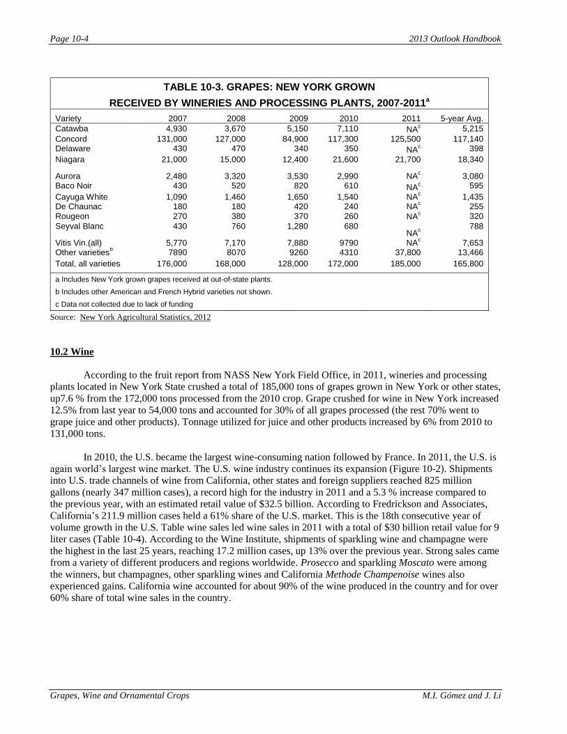
Page 10-4 2013 Outlook Handbook
Grapes, Wine and Ornamental Crops M.I. Gómez and J. Li
TABLE 10-3. GRAPES: NEW YORK GROWN
RECEIVED BY WINERIES AND PROCESSING PLANTS, 2007-2011a
Variety 2007 2008 2009 2010 2011 5-year Avg.
Catawba 4,930 3,670 5,150 7,110 NAc 5,215
Concord 131,000 127,000 84,900 117,300 125,500 117,140 Delaware 430 470 340 350 NA
c 398
Niagara 21,000 15,000 12,400 21,600 21,700 18,340
Aurora 2,480 3,320 3,530 2,990 NAc 3,080
Baco Noir 430 520 820 610 NAc 595
Cayuga White 1,090 1,460 1,650 1,540 NAc 1,435
De Chaunac 180 180 420 240 NAc 255
Rougeon 270 380 370 260 NAc 320
Seyval Blanc 430 760 1,280 680 NA
c
788
Vitis Vin.(all) 5,770 7,170 7,880 9790 NAc 7,653
Other varietiesb 7890 8070 9260 4310 37,800 13,466
Total, all varieties 176,000 168,000 128,000 172,000 185,000 165,800
a Includes New York grown grapes received at out-of-state plants.
b Includes other American and French Hybrid varieties not shown.
c Data not collected due to lack of funding
Source: New York Agricultural Statistics, 2012
10.2 Wine
According to the fruit report from NASS New York Field Office, in 2011, wineries and processing
plants located in New York State crushed a total of 185,000 tons of grapes grown in New York or other states,
up7.6 % from the 172,000 tons processed from the 2010 crop. Grape crushed for wine in New York increased
12.5% from last year to 54,000 tons and accounted for 30% of all grapes processed (the rest 70% went to
grape juice and other products). Tonnage utilized for juice and other products increased by 6% from 2010 to
131,000 tons.
In 2010, the U.S. became the largest wine-consuming nation followed by France. In 2011, the U.S. is
again world’s largest wine market. The U.S. wine industry continues its expansion (Figure 10-2). Shipments
into U.S. trade channels of wine from California, other states and foreign suppliers reached 825 million
gallons (nearly 347 million cases), a record high for the industry in 2011 and a 5.3 % increase compared to
the previous year, with an estimated retail value of $32.5 billion. According to Fredrickson and Associates,
California’s 211.9 million cases held a 61% share of the U.S. market. This is the 18th consecutive year of
volume growth in the U.S. Table wine sales led wine sales in 2011 with a total of $30 billion retail value for 9
liter cases (Table 10-4). According to the Wine Institute, shipments of sparkling wine and champagne were
the highest in the last 25 years, reaching 17.2 million cases, up 13% over the previous year. Strong sales came
from a variety of different producers and regions worldwide. Prosecco and sparkling Moscato were among
the winners, but champagnes, other sparkling wines and California Methode Champenoise wines also
experienced gains. California wine accounted for about 90% of the wine produced in the country and for over
60% share of total wine sales in the country.

2013 Outlook Handbook Page 10-5
M.I. Gómez and J Li Grapes, Wine and Ornamental Crops
Source: Wine Institute; Department of Commerce; Gomberg, Fredrickson and Associates, 2012
TABLE 10-4. WINE SALES IN THE U.S. 2007-2011 IN MILLIONS OF 9-LITER CASES
(Wine shipments from California, other states and foreign producers entering U.S distribution)
Year Table Wine Dessert Wine Sparkling Wine/
Champagne Total Wine Total Retail Value
2011 299.3 30.6 17.2 347.0 $32.5 billion
2010 285.2 29.1 15.4 329.7 $30.0 billion
2009 281.5 27.4 13.9 322.8 $28.7 billion
2008 274.7 27.6 13.5 315.8 $30.0 billion
2007 273.5 26.5 13.8 313.8 $30.4 billion
Source: Wine Institute; Department of Commerce; Gomberg, Fredrickson and Associates, 2012
U.S. wine exports, 90% from California, reached a new record of $1.39 billion in winery revenues in
2011, an increase of 21.7% from 2010. Volume shipments were up 5.8% to 455.7 million liters or 50.6
million nine-liter cases. 34% of U.S. wine exports by value were shipped to the 27-member countries of the
European Union, accounting for $478 million of the revenues, up 10% from 2010. Other top markets were:
Canada, $379 million, up 23%; Hong Kong, $163 million, up 39%; Japan, $105 million, up 39%; and China,
$62 million, up 42% (Figure 10-3).
825
519 526 543 568 574 617
639 665 692 717 745 753 767 784
0
100
200
300
400
500
600
700
800
1997 1998 1999 2000 2001 2002 2003 2004 2005 2006 2007 2008 2009 2010 2011
Total Table Wine Others
FIGURE 10-2. TOTAL WINE CONSUMPTION, U.S. 1997-2011 Million Gallons

Page 10-6 2013 Outlook Handbook
Grapes, Wine and Ornamental Crops M.I. Gómez and J. Li
Source: Wine Institute; Department of Commerce; Gomberg, Fredrickson and Associates, 2012
10.3 Outlook for Grapes and Wine
New York grapes are employed mostly in either wine or juice production, while a very small
percentage is allocated to table grapes. In 2011, there were 3,000 tons of fresh grapes, while 185,000 tons of
grapes were crushed by wineries and processors in New York State. According to USDA’s Economic
Research Service, the quantity of grapes to be crushed for wine is likely to go down in 2012-2013, mostly
driven by the reduced wine grape production in the state. The U.S. grape production is forecasted to have
smaller harvest than 2011 due to the unfavorable weather conditions this growing season, which affected
major producers particularly in Michigan, Ohio, Pennsylvania, and New York, where production reductions
are forecasted in the range of 35% to 75% from 2011 levels.
While deep production cuts are expected in many States, USDA forecasts suggests a steady
production in California, which supplies 90% of all U.S. grapes; and a significant boost in Washington, the
second-largest producer state. At the same time, dry weather has meant concentrated flavor and sugars and
reduction of pests and disease, translating into high-quality fruit. This may drive up prices growers will
receive for grapes sold to wineries through 2012/2013. The prices of wine on U.S. store shelves could start
rising this year because of an “emerging shortage” of wine grapes and wine plus a more intense wine
marketing last year.
Considering the grape juice market, after a significant increase in juice grape production from 2009 to
2010, the total quantity of grapes available for juice processing from this year’s harvested crop continued
increasing. This will likely drive down prices growers will receive from juice processors in 2012/13. In
addition, juice processors in the United States increased their international grape juice purchases by 3% from
the previous season. Grape juice exports from the U.S. are also forecasted to increase by 21.7%.
USDA forecasts that U.S. raisin production is likely to be down from the previous season. The
primary reason for this decline is the lower quantity of available grapes for drying this year and the forecasted
smaller harvest for raisin and table grapes in California. Grower prices for raisin grapes are expected to be
high due to reduced raisin production and tight inventories. Since the early 2000s, raisin grower prices
averaged at least $1,000 per ton. In 2011/12, prices averaged $1,632 per ton, up from $1,540 per ton in the
previous season and the highest since 2004. While this season’s domestic raisin production is anticipated to
34%
27%
12%
8%
4% 15%
EU
Canada
Hong Kong
Japan
China
Other
FIGURE 10-3. EXPORT OF U.S. WINE TO OTHER COUNTRIES 2011
2013 Outlook Handbook Page 10-7
M.I. Gómez and J Li Grapes, Wine and Ornamental Crops
decrease, exports of U.S. raisins in 2012/13 are forecasted to increase by 5% from last season to 360.0 million
pounds (dried weight). Raisin exports will increase primarily to Europe and China.
Table grape production is forecasted to drop again during the 2012-2013 marketing season. While
NASS forecast the State’s table grape crop to be slightly smaller this year, crop maturity moved ahead of last
year’s delayed crop, prolonged by cool, wet weather in the spring of 2011. U.S. grower prices for fresh grapes
averaged $0.705 per pound (or $1,410 per ton) in June, 31% higher than the June 2011 price, 68% above the
previous 5-year July average price, and the second highest July price on record since NASS started reporting
monthly grape prices in 1995. In addition to the anticipated reduced domestic table grape production, lower
overall imports from Chile this winter and spring likely contributed to strong early-season grower prices for
U.S. fresh grapes. Despite this decline, the current projected fresh production, if realized, will be relatively the
same as the previous 5-year average crop size. That should mean overall supply shortages in the U.S. fresh
grape market will not be an issue in 2012/13. California produces 90% of all U.S. grapes and supplies almost
all of production for fresh use. Domestic fresh grape use averaged 8.0 pounds per person over the previous 5
years (2007/08-2011/12).
Reduced grape production in California will be mostly behind the lower tonnage of U.S. grapes for
fresh use in 2012/13. Only a small volume of California wine grapes are diverted to the fresh market each
year. While raisin grapes are mostly used for raisin production, the volume of raisin grapes for fresh use far
exceeds those from wine grapes. Therefore, the decline in California’s raisin grape production would more
than offset the increase in the States’ wine grape production in reducing fresh-market supplies in 2012/13.
Based on the 2012/13 NASS forecast production, ERS projects U.S. fresh-market grape production to decline
for a second consecutive year to 1.92 billion pounds, down 2% from 2011/12.
Table 10-4 shows forecasts for the period 2013- 2015 from the National Food and Agricultural Policy
Project (NFAPP), prepared in 2010. According to NFAPP, total grape output will grow steadily. The
additional output is likely to be for wine and table grapes, as indicated by moderate increases in per capita
consumption of these two items. The juice grape projections present a pretty stable outlook, while the per
capita consumption of raisins shows a slightly downward trend.

Page 10-8 2013 Outlook Handbook
Grapes, Wine and Ornamental Crops M.I. Gómez and J. Li
TABLE 10-5. ECONOMIC OUTLOOK FOR GRAPES, 2013-2015
U.S. (unless noted otherwise)
2013 2014 2015
Total
Acres (1,000) 974 974 974
Yield (tons per acre) 8 8 8
Total U.S. Production (1,000 tons) 7,686 7,726 7,766
Total Production Outside California (1,000 tons) 876 905 938
Table Grapes
Production (million pounds) 2,045 2,069 2,093
Farm Price (dollars per ton) 775 805 838
Retail Price (dollars per pound) 2.44 2.54 2.64
Exports (million pounds) 912 938 957
Imports (million pounds) 1,500 1,557 1,614
Per capita consumption (pounds) 8.22 8.31 8.42
Wine
Production (million gallons) 641 651 662
Farm Price (dollars per ton) 678 711 746
Retail Price (dollars per gallon) 32.35 33.46 34.66
Exports (million gallons) 128 129 131
Imports (million gallons) 272 285 299
Per capita consumption (gallons) 2.45 2.5 2.54
Raisins
Production (million pounds) 677 681 685
Farm Price (dollars per ton) 221 223 226 Retail Price (dollars per pound) NA NA NA
Exports (million pounds) 360 368 376
Imports (million pounds) 48 51 54
Per capita consumption (pounds) 1.62 1.6 1.58
Grape Juice
Production (million gallons) 95 96 97
Farm Price (dollars per ton) 336 340 345
Retail Price (dollars per gallon) 4.7 4.82 4.96
Exports (million gallons) 28 29 29
Imports (million gallons) 83 85 88
Per capita consumption (gallons) 0.47 0.47 0.48 Source: National Food and Agricultural Policy Project, 2012.

2013 Outlook Handbook Page 10-9
M.I. Gómez and J Li Grapes, Wine and Ornamental Crops
10.4 Ornamentals
Nationally, the 2011 wholesale value of floriculture crops is down 2% from the revised 2010
valuation. The total crop value at wholesale for the 15-State program for all growers with $10,000 or more in
sales is estimated at $4.08 billion for 2011, compared with $4.15 billion for 2010. The number of producers
for 2011 is 5,763, which represents a reduction of 7% from the previous year. The total covered area for
floriculture crop production was 71 million square feet, which is down 2% from 2010.
TABLE 10-6. GROWER CASH RECEIPTS OF FLORICULTURE AND NURSERY CROPS, NEW YORK, 2005-2011
2005 2006 2007 2008 2009 2010 2011
--- Million dollars ---
Floriculturea.b
200.6 203.5 209.1 204.3 182.6 166.6 171.2
Nurseryc 181.3 205.5 NA NA NA NA NA
Floriculture and nursery crops 381.9 409 NA NA NA NA NA
a Includes growers with $10,000 or more in floriculture sales.
b Includes ornamental plants without woody stems, grouped into bedding/garden plants, cut cultivated greens, cut flowers, potted flowering plants, indoor foliage plants, and propagative floriculture material.
c Includes ornamental plants and trees with woody stems, including broadleaf evergreens, coniferous evergreens, deciduous shade trees, deciduous flowering trees, deciduous shrubs and other ornamentals, fruit and nut plants for home use, cut and to-be-cut Christmas trees, and propagation material or lining-out stock. Also includes other ornamental crops not classified as floriculture.
NA Not available
Source: Floriculture and Nursery Press Release, National Agricultural Statistical Service. 2012
TABLE 10-7. VALUE OF FLORICULTURE PRODUCTION BY PLANT CATEGORY,
NEW YORK, 2007-2011
2007 2008 2009
2011 vs.
5-yr. avg.
2011 vs.
2010
5-yr. avg.
2007-2011
2010 2011
% %
Bedding/garden plantsa 111.8 109 98.6 105 103 105.5 -2.3% -1.9%
Potted flowering plantsa 41.4 42 42.3 20.8 24.2 34.1 -29.1% 16.3%
Cut flowersa 4.6 NA 2.3 1.9 NA
c 2.9 NA NA
Foliage Plantsa 3.3 4.2 2.94 2.63 NA
c 3.3 NA NA
Propagative materialsa 20.7 19.8 16.8 17.6 22.1 19.4 13.9% 25.6%
Grower sales 27.1 26.4 17.7 18.9 19.6 21.9 -10.7% 3.7% $10,000-$99,999 (Unspecified crops)
Totalb 209.1 204 183 167 171 186.8 -8.3% 2.8%
a Sales by operations with annual sales of $100,000 or more. b
Total reported crops includes categories not listed
c Not published to avoid disclosing individual operations
Source: Floriculture and Nursery Crops, Situation and Outlook Yearbook, Economic Research Service, USDA, various years.
In 2011, the commercial sales value of New York floriculture production totaled $171 million, a
slightly increase from the revised 2010 sales value, ranking New York 8th in the nation (Table 10-6).

Page 10-10 2013 Outlook Handbook
Grapes, Wine and Ornamental Crops M.I. Gómez and J. Li
Unfortunately, data on nurseries is not available after 2006, due to changes in data collection procedures at
USDA’s National Agricultural Statistical Service, thus this situation analysis considers only floriculture.
Table 10-7 indicates that bedding and garden plants are the number one component with total value of sales at
$103million in 2011, a slightly decrease from the revised 2010 sales value. Potted flowering plants were
second with a value of sales of $24.2 million in 2011, a significant decrease from 2009. Propagative materials
were third at $22.121 million, a 26% increase from the previous year (Table 10-6). In 2010, there were 615
growers in New York (down from 657 in 2010) and the open ground area used to produce floriculture crops
kept decreasing to 670 acres, down 12% from 2010 (Table 10-7). However, according to the NYS Department
of Agriculture and Markets, these data on open ground area are not comparable to previous years due to the
combined data collection efforts of the Census of Horticulture and the Annual Floriculture Survey. The data
in 2011 include area used for production of nursery crops as well as floriculture crops.
TABLE 10-8. GROWING AREA FOR FLORICULTURE CROPS IN NEW YORKa
2007-2011
Year
Total Shade and Total covered
area Open ground Total covered & open ground greenhouse temporary
cover cover
-- 1,000 square feet -- --- acres ---
2007 25,619 705 26,324 1,068 1,673
2008 23,473 531 24,404 1,382 1,943
2009 23,042 405 23,447 2,589 3,127
2010b 25,378 340 25,718 760 1,350
2011 25,023 286 25,309 670 1,250 a Includes operations with $10,000+ in annual floriculture sales. Crops include cut flowers, cut cultivated greens, potted flowering plants, potted foliage plants, bedding and garden plants, and propagative materials. Total may not add due to rounding.
b Revised
Source: Floriculture Crops, NASS, USDA, various years
An important distinction in floricultural production is the size of operation. According to NASS
reports, the U.S. value of floriculture production was $4.08 billion in 2011, compared to $4.13 billion for
2010 (Table 10-9). The value of production from large and small growers decreased by 1.1% and by 4% with
respect to 2010, respectively. While the value of production from large and small growers in New York both
increased by 2.6% and 3% from 2010, respectively. The share of value of production from small growers is
larger in New York in comparison to the national market. Small growers’ share of production in New York is
11.4%, which is high compared to the 3.5 % in the U.S. In New York, the value of production from small
growers increased to $19.6 million in 2011 from 2010; and the value from large growers increased slightly to
$ 151.6 million relative to 2010 (Table 10-9).
When reading the published U.S. floriculture and nursery crop statistics, it should be noted that only
15 states were surveyed by the USDA in 2006 and thereafter, compared to 36 states prior to 2006.
Consequently, the 2004-2005 data in Table 10-9 were adjusted to include only the 15 states surveyed in 2009
and 2010 for comparison. In 2011, the leading state is still California which accounts for 25% of the total
wholesale value in the 15-States. Florida ranks second with 21%; while Michigan ranks third with 9%, and
Texas and North Carolina round out the top 5 accounting for 6% each.
According to the Floriculture Crop 2011 summary report by NASS, USDA, the 2011 wholesale value
of floriculture crops is down 3.94% compared to 2010. The crop value at wholesale for growers with $10,000

2013 Outlook Handbook Page 10-11
M.I. Gómez and J Li Grapes, Wine and Ornamental Crops
or more in sales is estimated at $3.94 billion for 2011, compared with $3.98 billion for 2010. Bedding and
Garden plants wholesale value of bedding and garden plants, at $1.91 billion, is down about 2% from the
previous year. Potted flowering plants for indoor or patio use, were valued at $640 billion in 2010, down 1%
from 2010. The value of 2010 foliage plant production, at $613 million, is up 5% from the previous year,
Florida continues to dominate this category with 72% of the total value. The value of cut flowers, at $359
million, is 4% less than 2010; while cut cultivated greens, shrinks to72 million from $78 million in 2010.
TABLE 10-9. WHOLESALE VALUES OF FLORICULTURE PRODUCTION,
BY GROWER SIZEa, NEW YORK AND UNITED STATES, 2009-2011b
New York
U.S.
2009 2010 2011 2009 2010 2011
------ Million dollars ------
Small growers 17.3 19.0 19.6
140 150 144
Large growers 153.2 147.7 151.6
3,860 3,980 3937
All growers 170.5 166.7 171.2 4,000 4,130 4081 a Small growers have between $10,000 and $100,000 in annual floriculture sales; large growers have at least $100,000.
b Wholesale value of sales of growers with at least $10,000 in annual floriculture sales. Growers are located in the 36 surveyed states.
Source: Floriculture Crop, National Agricultural Statistic Service (NASS), USDA, 2011
Regarding nursery crops, after several dismal sales in recent years, it seems that some relief has
finally surfaced. Nursery Management (2012) surveyed growers in the states of Ohio, Indiana, Illinois,
Wisconsin, Michigan, Kentucky, West Virginia and Virginia. The survey compared nursery performance in
2012 versus 2011. The majority of growers indicated an increase in sales and in profitability in 2012 relative
to 2011. The survey reveals that about 30% of growers currently have a profit margin between 11-15%;
nearly 20% of growers enjoyed profit margins ranging from 1 to 5 %; and 20% of growers reported profit
margins above 25% in 2012 (Figure 10-4). The analysis indicates that more than 40% of those surveyed
predicted a 6-10% growth in sales in 2012; 30% of growers are expecting a 1-5% sales growth; and more than
10% of growers are forecasting a 21-25% increase in sales.
Source: Nursery Management, 2012
Less than 1%
1-5%
6-10%
11-15%
16-20%
21-25%
More than 25%
FIGURE 10-4. THE PROFIT MARGIN, ON AVERAGE

Page 10-12 2013 Outlook Handbook
Grapes, Wine and Ornamental Crops M.I. Gómez and J. Li
Many growers in the north/central region of the U.S. already have or will plant more this year
compared to 2011(Table 10-10). The majority of respondents said they planned to increase production by 1-
10%. This is good news, in comparison to the negative trends experienced by the sector in recent years.
Increased production varies by the type of product: about 12% of those surveyed are increasing deciduous
shade and flowering trees by more than 50%; nearly 36% of growers are planning to increase production of
propagated materials by more than 26% in 2012; and 15% of growers plan to increase production of
evergreen trees by more than 25%. Overall, growers are very confident that the tree business will grow, they
believe that the demand will be strong, and predict that prices will be high.
TABLE 10-10. CROPS THAT GROWERS ARE INCREASING PRODUCTION IN 2012 VS 2011
PRODUCT 1-10% 11-25% 26-50% MORE THAN 50%
Deciduous shade and flowering trees 48.0% 40.0% 0.0% 12.0%
Herbaceous Perennials 71.4% 23.8% 0.0% 4.8%
Deciduous Shrubs 78.3% 17.4% 0.0% 4.3%
Propagated Material (liners, cuttings, plugs) 28.6% 35.7% 28.6% 7.1%
Evergreen Trees 53.8% 30.8% 7.7% 7.7%
Source: Nursery Management, 2012
Outlook
Economic indicators suggest that ornamental growers are recovering from the economic downturn
and experiencing a period of steady sustained growth. The predictions for 2013 are that we will experience a
period of sluggish growth with a slow recovery in the next few years. The production of the ornamental crops
will increase in the coming 2013, which is primary because the market is experiencing some kind of shortage
throughout much of the U.S as growers have cut production, including but not limited to bedding plants field-
grown material and shade trees. At the same time, there is growing interest from a large number of
households in re-investing in their current landscapes. Therefore the short supply and the expected demand
increase will probability provide the right incentives to recover the growth path of the ornamental industry.
However, the growers need to be cautious to expand since they have been hit hard in the past four years. The
implications for the floriculture industry and for nurseries and landscape industries are therefore cautiously
optimistic.
With the shortages in the supply of ornamental products in the near future, it will be more critical
than ever for retailers to commit for product purchases earlier and with firm purchase orders, especially for
peak selling periods. Pre-books will need to be the norm rather than the exception. Retailers and suppliers are
in need of strengthening their partnerships by sharing information with each other so as to gain market
knowledge and benefit from supply chain efficiencies.
The next couple of year won’t be more challenging than the past several years. However, to
maintain growth, suppliers should focus on understanding customer needs and on having the right assortment
of products. They need to learn to serve customers in innovative ways: as consumers continue to change, they
need to change with them. Producers and retailers should not try to wait to react to change. Instead they
should focus on anticipating consumer demand for the products and services offered by the industry. By
doing so, the ornamental supply chain, including growers and retailers, would eventually be more customer-
centered, more relationship-oriented, and more transparent.
2013 Outlook Handbook Page 10-13
M.I. Gómez and J Li Grapes, Wine and Ornamental Crops
Looking ahead, the industry is in need of identifying key consumer benefits that could be promoted
either by individual firms or by ornamental industry national and regional associations. This could be through
aggressive industry marketing strategies based on promotions, publicity, branding, and product innovation.

Notes
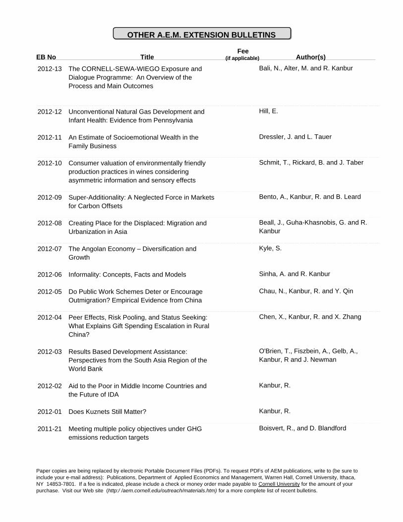
EB No Title Author(s)
OTHER A.E.M. EXTENSION BULLETINS
Fee(if applicable)
The CORNELL-SEWA-WIEGO Exposure andDialogue Programme: An Overview of theProcess and Main Outcomes
Bali, N., Alter, M. and R. Kanbur2012-13
Unconventional Natural Gas Development andInfant Health: Evidence from Pennsylvania
Hill, E.2012-12
An Estimate of Socioemotional Wealth in theFamily Business
Dressler, J. and L. Tauer2012-11
Consumer valuation of environmentally friendlyproduction practices in wines consideringasymmetric information and sensory effects
Schmit, T., Rickard, B. and J. Taber2012-10
Super-Additionality: A Neglected Force in Marketsfor Carbon Offsets
Bento, A., Kanbur, R. and B. Leard2012-09
Creating Place for the Displaced: Migration andUrbanization in Asia
Beall, J., Guha-Khasnobis, G. and R.Kanbur
2012-08
The Angolan Economy – Diversification andGrowth
Kyle, S.2012-07
Informality: Concepts, Facts and Models Sinha, A. and R. Kanbur2012-06
Do Public Work Schemes Deter or EncourageOutmigration? Empirical Evidence from China
Chau, N., Kanbur, R. and Y. Qin2012-05
Peer Effects, Risk Pooling, and Status Seeking:What Explains Gift Spending Escalation in RuralChina?
Chen, X., Kanbur, R. and X. Zhang2012-04
Results Based Development Assistance:Perspectives from the South Asia Region of theWorld Bank
O'Brien, T., Fiszbein, A., Gelb, A.,Kanbur, R and J. Newman
2012-03
Aid to the Poor in Middle Income Countries andthe Future of IDA
Kanbur, R.2012-02
Does Kuznets Still Matter? Kanbur, R.2012-01
Meeting multiple policy objectives under GHGemissions reduction targets
Boisvert, R., and D. Blandford2011-21
Paper copies are being replaced by electronic Portable Document Files (PDFs). To request PDFs of AEM publications, write to (be sure toinclude your e-mail address): Publications, Department of Applied Economics and Management, Warren Hall, Cornell University, Ithaca,NY 14853-7801. If a fee is indicated, please include a check or money order made payable to Cornell University for the amount of yourpurchase. Visit our Web site (http:/ /aem.cornell.edu/outreach/materials.htm) for a more complete list of recent bulletins.