New results on single-machine two-agent scheduling problems

Alessandro Agnetis, Università di Sienajoint work with

Gianluca De Pascale, Università di Siena Dario Pacciarelli, Università di Roma Tre

Marco Pranzo, Università di Siena

CIRM, Marseille 12/5/2008

Multi-agent problems

• A set of m agents, each owning a set of jobs

• Job j requires processing time pj

• There is a single machine

• Each agent k wants to minimize a cost function f k() which only depends on the schedule of his/her jobs

• Trains competing for railroad resource usage [Brewer and Plott 1996]• Quay cranes at container terminals competing for movers [Lau et al 2007]• Allocation of airport time slots to incoming aircraft [Ball et al. 2000]

• Resource allocation in industrial districts[Albino, Carbonara and Giannoccaro 2006]• Schedule adjustment upon arrival of new jobs

[Leung, Pinedo and Wan 2007]

• Different data packets competing for radio resources [Meiners and Torng 2007]

• Protocols– Auction mechanisms (Wellman et al

2002)– Combinatorial auctions (Kutanoglu and

Wu 1999, Lau et al 2007) – Automated protocols (Fink 2006)

• Cooperative/Noncooperative games– Sequencing games (Curiel et al 1989)– Decentralization cost, mechanism design

(Hain and Mitra 2006, Bukchin and Hanany 2007)

• Bargaining models, multi-agent scheduling– Nash (1950), Mariotti (1998), Peha

(1995), A. et al (2004, 2007), Baker and Smith (2003), Arbib et al (2005), Cheng, Ng, Yuan (2006, 2007), Leung, Pinedo and Wan (2007), Meiners and Torng (2006)

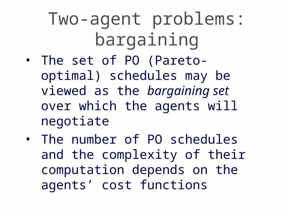
Two-agent problems: bargaining

• The set of PO (Pareto-optimal) schedules may be viewed as the bargaining set over which the agents will negotiate

• The number of PO schedules and the complexity of their computation depends on the agents’ cost functions

-constrained problem

• The problem is to compute the schedule which minimizes the cost for agent A such that the cost for B does not exceed Q

• By varying Q, one can generate all PO schedules

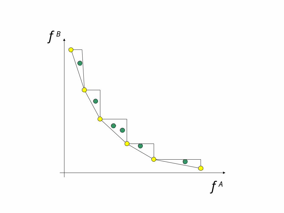
f B

f A

Agents’ utility

• The bargaining set also contains a point (dA,dB) representing the agents’ utility if negotiation fails (disagreement point)

• We consider the agents’ utilitiesuA()=d A – f A()uB()=d B – f B()

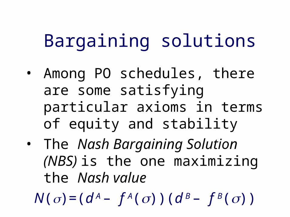
Bargaining solutions

• Among PO schedules, there are some satisfying particular axioms in terms of equity and stability

• The Nash Bargaining Solution (NBS) is the one maximizing the Nash valueN()=(d A – f A())(d B – f B())

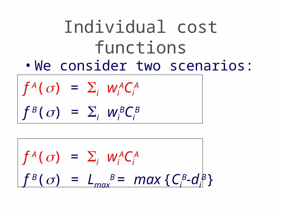
Individual cost functions

• We consider two scenarios:

f A() = i wiACi

A

f B() = i wiBCi

B

f A() = i wiACi

A

f B() = LmaxB = max {Ci

B-diB}

1| i wiBCi

B Q | i wiACi

A

Complexity

• The -constrained problem is NP-hard, even if all jobs have equal weights

• The number of PO schedules is pseudopolynomial

• Finding the Nash solution is also NP-hard (A., de Pascale and Pranzo 2007)

min i wiACi

A ()

i wiBCi

B () Q S

• If we relax the constraint, we get the Lagrangian problem:

L() = min i wiACi

A () + (i wiBCi

B () - Q)

S

Lagrangian relaxation

• The Lagrangian problem is simply solved by ranking the jobs in nondecreasing order of k where

kA = wk

A/ pkA if k A

kB = wk

B / pkB if k B

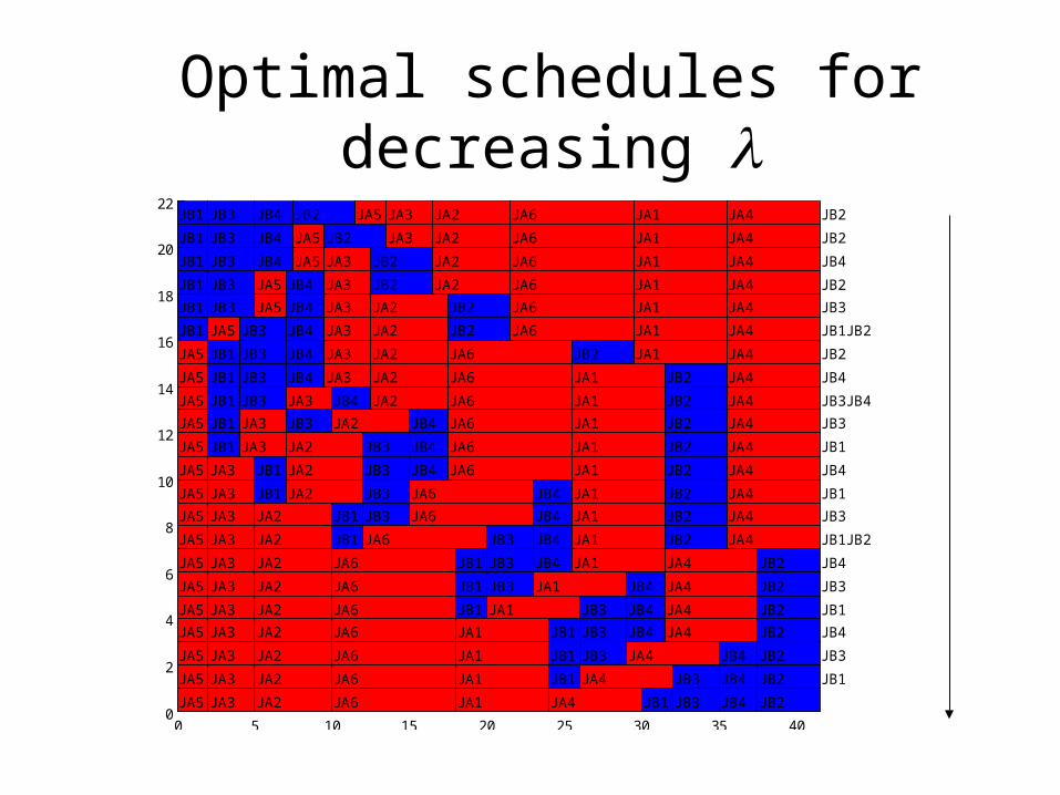
Optimal schedules for decreasing

0 5 10 15 20 25 30 35 400

2

4

6

8

10

12

14

16

18

20

22JB1 JB3 JB4 JB2 JA5 JA3 JA2 JA6 JA1 JA4 JB2

JB1 JB3 JB4 JA5 JB2 JA3 JA2 JA6 JA1 JA4 JB2

JB1 JB3 JB4 JA5 JA3 JB2 JA2 JA6 JA1 JA4 JB4

JB1 JB3 JA5 JB4 JA3 JB2 JA2 JA6 JA1 JA4 JB2

JB1 JB3 JA5 JB4 JA3 JA2 JB2 JA6 JA1 JA4 JB3

JB1 JA5 JB3 JB4 JA3 JA2 JB2 JA6 JA1 JA4 JB1JB2

JA5 JB1 JB3 JB4 JA3 JA2 JA6 JB2 JA1 JA4 JB2

JA5 JB1 JB3 JB4 JA3 JA2 JA6 JA1 JB2 JA4 JB4

JA5 JB1 JB3 JA3 JB4 JA2 JA6 JA1 JB2 JA4 JB3JB4

JA5 JB1 JA3 JB3 JA2 JB4 JA6 JA1 JB2 JA4 JB3

JA5 JB1 JA3 JA2 JB3 JB4 JA6 JA1 JB2 JA4 JB1

JA5 JA3 JB1 JA2 JB3 JB4 JA6 JA1 JB2 JA4 JB4

JA5 JA3 JB1 JA2 JB3 JA6 JB4 JA1 JB2 JA4 JB1

JA5 JA3 JA2 JB1 JB3 JA6 JB4 JA1 JB2 JA4 JB3

JA5 JA3 JA2 JB1 JA6 JB3 JB4 JA1 JB2 JA4 JB1JB2

JA5 JA3 JA2 JA6 JB1 JB3 JB4 JA1 JA4 JB2 JB4

JA5 JA3 JA2 JA6 JB1 JB3 JA1 JB4 JA4 JB2 JB3

JA5 JA3 JA2 JA6 JB1 JA1 JB3 JB4 JA4 JB2 JB1

JA5 JA3 JA2 JA6 JA1 JB1 JB3 JB4 JA4 JB2 JB4

JA5 JA3 JA2 JA6 JA1 JB1 JB3 JA4 JB4 JB2 JB3

JA5 JA3 JA2 JA6 JA1 JB1 JA4 JB3 JB4 JB2 JB1

JA5 JA3 JA2 JA6 JA1 JA4 JB1 JB3 JB4 JB2

0 0.5 1 1.5 2 2.5 3 3.5180

200

220

240

260

280

300

320

340

PO schedules and NBS

• The Lagrangian bound is used in a branch and bound algorithm to generate PO schedules

• To find the NBS, we adopt the approach:– Generate all extreme schedules– Locate the triangle containing the

NBS– Enumerate PO solutions in the

triangle

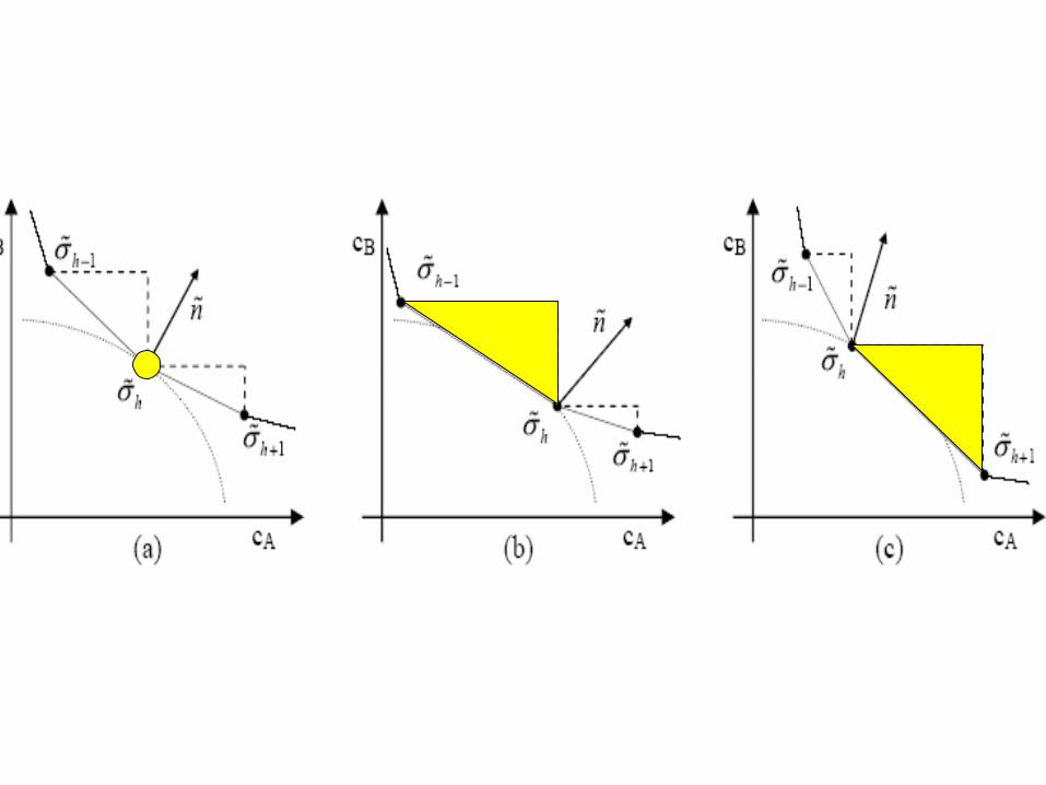
Locating the Nash triangle

• The Nash triangle can be found evaluating the angle between the convex hull of extreme schedules and the gradient of the Nash function

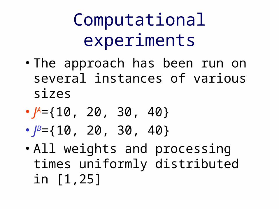
Computational experiments

• The approach has been run on several instances of various sizes

• JA={10, 20, 30, 40} • JB={10, 20, 30, 40}• All weights and processing times

uniformly distributed in [1,25]

nA nB |E| |PO| T1 TPO TNASH

10 10 60 603 0.01 4 0.0610 20 119 4595 0.05 217 1.7210 30 178 15383 0.14 2185 12.3010 40 232 74771 0.32 24061 102.2720 10 118 4698 0.05 227 1.862020 239 15601 0.14 2110 8.9620 30 345 74547 0.33 24912 69.2120 40 451 220000 0.65 146400 322.87

30 10 178 15413 0.14 2120 12.4830 20 346 75225 0.31 22883 65.2430 30 510 219000 0.64 140700 282.5830 40 662 950000 1.12 1056000 1571.23

40 10 233 73952 0.33 24427 110.2340 20 452 220000 0.63 138000 311.0640 30 653 947000 1.09 1062000 1551.5540 40 862 2397000 1.81 4218000 4974.83

1| LmaxB Q | i wi

ACiA

1|LmaxB Q | i wi

ACiA

min i wiACi

A ()

C1B() Q1

B

C2B() Q2

B

……CnB

B() QnBB

S

Complexity

• The -constrained problem is strongly NP-hard (A. et al 2004, Cheng,Ng and Yuan 2006)

• The number of PO schedules is pseudopolynomial

• Even finding extreme schedules is NP-hard (Baker and Smith 2003, Hoogeveen 2002)

Lower bounds

• The problem is a special case of

1|dj | jwjCj

• Pan (2003) solves instances with up to 100 jobs, based on a bounding approach by Posner (1995)

Example

Agent A

f A= iwiCi

i pi wi

X 2 4 Y 3 5 Z 3 4

Agent B

f B= Lmax B

i pi di

K 2 6

Optimal solution

6

3 7 10

Y X Z

5 44

5 * 3 + 4 * 7 + 4 * 10 = 83

Posner’s preemptive bound

6

2 7 10

X Z

4 45 * 2/3

4 * 2 + 10/3 * 4 + 5/3 * 7 + 4 * 10 = 73

Y1 Y2

5 * 1/3

4

weights

Lagrangian relaxation

• Relaxing all the constraints, one has

L() =

min i wiACi

A () + j j(CjB() - Qj

B)

S

Lagrangian relaxation

• The Lagrangian problem is solved by ranking the jobs in nondecreasing order of j where

iA = wi

A/ piA if i A

kB = k

/ pkB if k B

Lagrangian dual

• Theorem In an optimal solution to the Lagrangian dual, for each B-job k there exists an A-job i such that

k*B = iA

Structure of an optimal solution of the Lagrangian

dual

4 2.5 2.5 2.5 2.5 2.5 1 1 1

Values of

Note: the ordering within each cluster is immaterial

Solving the Lagrangian dual

• To solve the Lagrangian dual, we only need to find the partition of the B-jobs

• Let Rj := QjB - pj

B

• The window of a B-job is the time span [Rj

, Qj ]

4 2.5 1

Windows

2.5

4 2.5 1

Windows

2.5 2.5

4 2.5 1

Windows

2.5 2.5 1

Lagrangian bound

• Theorem The bound provided by the optimal solution to the Lagrangian dual dominates Posner’s bound

Lagrangean bound

6

2 7 10

X Z

4 42 * 5/3

4 * 2 + 5 * 7 + 4 * 10 + 2*(5/3)*(-2) = 76.333

Y

5

4

weights

Conclusions…• The Lagrangian approach

appears viable for efficiently deriving good lower bounds for these classes of two-agent scheduling problems

• The number of PO schedules may grow rapidly, but the NBS can still be computed in reasonable time

• The “best” extreme schedule approximates the NBS very well

…and future research

• Extension to other cost functions

• Simulations to compare bargaining vs. auction-type approaches

• Other decentralized protocols