DesignCon 2015

New Metric Offers More

Accurate Estimate of Optical

Transmitter’s Impact on

Multimode Fiber-optic Links

John Petrilla, Avago Technologies

Piers Dawe, Mellanox Technologies

Greg D. Le Cheminant, Keysight Technologies

Abstract

Reliable metrics to define and quantify performance of transmitters used in high-speed

optical communications have been historically difficult to achieve. The classic eye-mask

test provides a coarse method to screen out bad devices, but is not an accurate predictor

of system level performance in terms of bit error ratio (BER). Transmitter and dispersion

penalty (TDP) analysis yields a BER-based metric, but is complicated and expensive to

perform. A recent IEEE Ethernet project (802.3bm) has developed a new signal quality

metric, TDEC (transmitter and dispersion eye closure), for multimode optical transmitters

that seeks to provide a simple and low cost test method that reliably predicts operation

when deployed with standards-compliant channels and receivers. In this paper we

discuss the limitations of the existing metrics and present the new TDEC metric and its

expected advantages. Methods to implement the new measurement in standard

instrumentation and actual measurement results will be reviewed.

Authors Biographies

John Petrilla is a Development Engineer in the Product Strategy & Architecture group of

Avago Technologies, Fiber Optic Products Division. He participates in new product

definition and represents Avago Technologies in several industry standards and multi-

source agreement groups. He has been employed since 1977 by Hewlett-

Packard/Agilent/Avago in various product development activities. John earned a BEE

degree from the University of Detroit and a MSEE degree from Santa Clara University

and holds nine patents.

Piers Dawe is Senior Staff Engineer, analog link architect and standards, for Mellanox

Technologies. He represents Mellanox Technologies in several industry standards groups.

His career in fiber optics and semiconductors began at STL (later BNR then Nortel) and

continued at Hewlett-Packard/Agilent/Avago then IPtronics, now part of Mellanox. He

has made major contributions to standards such as 802.3ae, SFP+ and 802.3ba, including

the 10 gigabit Ethernet link model and hit ratio mask measurement. He has an MA degree

from the University of Cambridge, has contributed to around 20 refereed publications,

and holds 11 patents.

Greg Le Cheminant is a Measurement Applications Specialist for digital communications

analysis products in the Oscilloscope Products Division. He is responsible for product

management and development of new measurement applications for the division's digital

communications analyzer and jitter test products. He represents Keysight on several

industry standards committees. Greg's experience at Keysight/Agilent/Hewlett-Packard

began in 1985 with five years in manufacturing engineering, and the remainder in various

product marketing positions. He is a contributing author to four textbooks on high-speed

digital communications and has written numerous technical articles on test related topics.

He holds two patents. Greg earned BSEET and MSEE degrees from Brigham Young

University.

.

Developing specifications for lower cost fiber optic

links

Networks, as well as becoming more valuable as the number of users (network nodes)

increase, are more valuable when a wide range of suppliers are enabled. The challenge is

to ensure that functions from that wide range of suppliers operate together in a

satisfactory manner. Cost is also a major consideration as a network comprising low cost

elements is more likely to be widely accepted and used. It is especially attractive when

network elements can be simply plugged together and work without operator adjustment,

i.e. “plug and play”.

An approach to ensure interoperation is to group various elements and/or functions into

blocks and define the blocks by the signals that pass between blocks. The OSI Reference

Model provides an example of such an approach.

Specifications can then be written at a component level or at a system level. At a

component level, a component is assumed to be isolated (inputs and outputs of the

component are available) and tests can be defined to ascertain that the inputs have the

required characteristics, the outputs have the required characteristics and the outputs have

the required response to the inputs. A wide variety of test equipment and test patterns

can be employed. However another step at a higher level is required to assure that the

combined components support the requirements of the system. This approach can result

in a large number of requirements and associated tests.

Specifications written at a system level are constrained by which interfaces are exposed

and the operations that the system provides. Thorough testing may require that systems

provide special signals and/or test patterns that are only used for testing. An advantage is

that the system can be used to determine the adequacy of the function under test, e.g. are

errors being generated and/or detected. This paper will mainly address optical elements

of Ethernet or similar networks, focusing on minimum signal and maximum impairment

cases for multimode fiber channels.

Within Ethernet networks, specifications are nominally written at the system level.

Relevant entities for this paper include functional blocks Physical Medium Dependent

(PMD) blocks and the optical medium, here multimode fiber (MMF), and the interface

(Medium Dependent Interface, MDI) between the PMD and medium. Requirements can

be defined for the signal launched into the medium from an optical transmitter (Tx) and

for the signal exiting the medium and incident on the optical receiver (Rx). In an

Ethernet environment, optical connectors are expected at the interface between the Tx

and medium and at the interface between the medium and the Rx. Since the signals of

interest can be exposed at these connectors, these are good choices for compliance points.

However, since it is the signal launched into the fiber that is of interest, the Tx output is

measured at the output of a short patch cord that is connected into the Tx.

Before interoperation between optical transmitters and receivers is addressed, operation,

specifically minimally acceptable operation, should be defined. Simplistically, this

would include, at a minimum, the bit error ratio (BER) for a given data rate, type and

reach of a medium (cable plant), optical wavelength and spectral characteristics, signal

modulation and encoding, bandwidth, signal amplitude and noise level requirements. A

model of the optical channel comprising an optical transmitter, an optical cable plant and

an optical receiver, with sufficient detail can be used to reach agreement among

stakeholders of a combination of minimally acceptable transmitters, cable plant and

receivers that, in combination, provides an acceptable level of performance and accounts

for all expected impairments. Such a model can then be used to estimate the signal

characteristics at the interfaces of interest so that signal requirements can be defined at

these interfaces 1,2,3

.

To ensure interoperation one approach can be to constrain the transmitter, medium and

receiver attributes such that all combinations of worst case transmitters, worst case

receivers and worst case media operate satisfactorily without adjustment. Simply stated,

satisfactory operation can be defined as the system operating at less than a maximum bit

error ratio (BER) requirement. A variant of this approach is for the Rx to adapt to a less

constrained Tx and medium. Another approach is to allow even fewer constraints and

provide a means for the Tx and Rx to communicate such that the Tx and Rx can negotiate

and adapt to the medium and each other. Plug and play does not preclude self adaption or

mutual adaption.

Unfortunately even these relatively simple models contain upwards of thirty

characteristics and assumptions – too many to include as explicit requirements if low cost

tests and components are desired. Consequently, attributes that aggregate the more

detailed characteristics are desired. Ideally, there would be a single global transmitter

output attribute and a single global receiver attribute. Fortunately link models can

convert signal impairments into power penalties and, operating as budgets, combine

individual penalties into aggregates.

It is helpful in a search for such global attributes to shift from thinking of individual

signal characteristics to thinking of operational results. For example, how badly can an

impaired Tx affect a receiver’s ability to recover a signal before performance is

unacceptable (acceptable is usually in terms of system BER)? Any Rx device under test,

DUT, that can recover a signal from a worst case Tx through a worst case medium is

acceptable. Likewise, any Tx DUT that can provide a signal through a worst case

medium and have the signal recovered by a worst case Rx is acceptable. This appears to

require access to a worst case Tx, a worst case Rx and a worst case medium. While worst

case devices (transmitters and/or receivers) may be difficult to generate, a reference

device (transmitter and/or receiver) with well-defined difference in performance relative

to the worst case transmitter and/or receiver may be possible. A shift away from a worst

case Rx, where the test of a Tx is a pass-fail event (if the worst case Rx recovers the data

the Tx DUT passes, if not it fails) requires a knowledge of the margin between the

reference receiver, (Ref Rx), and the worst case Rx and the test of the Tx DUT becomes

the measure of the margin degradation it causes in the Ref Rx and its comparison with

that of the worst case Tx.

When such global attributes are available, there is another advantage. The individual

attributes can now trade-off with each other offering a yield advantage with no

degradation in specified worst case performance. For example, instead of a single worst

case Tx combination of several attributes, there is a family of worst case transmitters; all

yielding the same value for the global attribute. This permits manufacturers to take

advantage of what they each can do best.

Since various optical medium characteristics interact with various Tx characteristics, a

worst case medium is essential. For example, with multimode fiber (MMF) the

deleterious effect of the fiber‘s chromatic dispersion depends on the spectral width of the

optical source. While for single-mode fiber (SMF), since only a single mode is supported

in the fiber, a worst case fiber can be found where the characteristics of the fiber and

signal launched into the fiber are constrained, for MMF and multimode sources slight

differences in launch condition can, for example lead to significant differences in

effective fiber bandwidths, even for the multiple matings of the transmitter-fiber pair.

What is required to ensure interoperability?

For multimode, since there is little confidence in the availability of a worst case fiber, the

wavelength and spectral width of the Tx are separately tested to assure they are within

requirements. To assure fiber modal bandwidth, BW, the launch pattern of the Tx is

constrained by the Encircled Flux requirement. A minimum Extinction Ratio, ER, may

be required to constrain noise penalties that are allocated and/or not captured in other

measurements. Not critical for MM devices is the Optical Return Loss, except as a

condition for RIN (Relative Intensity Noise) tests. An eye mask is often used to provide

an estimate of the signal quality of the Tx output, but while it can be used as a screen for

aberrant waveforms such as those with excessive overshoot and ringing, the limited

amount of data that can be collected in a reasonable test time is not suitable to assure

common bit error ratios to probabilities in the magnitude of 10-12

.

For receivers, the Rx signal rate, optical wavelength, modulation and signal levels must

be defined. The global test consists of conditioning a signal to match a worst case signal

expected from a worst case Tx coupled through a worst case fiber cable. Here a model

can be used to predict the impairments generated by the combination of the worst case Tx

and cable plant. Test equipment can then be used to generate these impairments in an

otherwise clean signal. Consequently, there is no need for an actual worst case Tx or

worst case fiber.

Another consideration: Increasing signal rates and instrument

noise

As data rates increase, maintaining signal integrity becomes more difficult. A point is

eventually reached where the link is no longer able to achieve the desired BER while at

the same time the increasing signal rate leads to a need for a lower BER in order to

maintain, e.g. a target errors per day metric. For a given channel length the transmitted

signal experiences sufficient loss and/or distortion so that the receiver will make mistakes

at a rate that cannot be tolerated by the system using the link. If data rate and channel

span are fixed, system design may require more elaborate coding schemes to achieve a

system level BER improvement. Thus a system with a link BER of 10-6

can have the

desired system BER of 10-12

. Forward error correction (FEC) schemes are commonly

used to achieve this.

The historic BER requirement of 10-12

in many Ethernet links required test methods that

were able to confirm performance at similar levels of probability. Validation to this low

level requires either an extensive amount of data, or an accurate method to extrapolate

smaller data sets to low probabilities. If the link hardware is able to operate at a higher

BER, test methods experience some possible relief as smaller data sets are required to

verify performance. Direct analysis of eye diagram waveform statistics can now be used

to estimate how well the transmitter will perform within a link.

Contenders for a global transmitter attribute:

Several candidates Tx Output Eye-Mask, Eye Width and Eye Height, TDP and TDEC,

for a global Tx metric will be considered. All of these are relative metric. Consequently

an absolute value amplitude metric, Tx Output OMA, is required with each to ensure a

sufficient signal amplitude.

Transmitter Output Eye Mask Tests

The eye diagram displays multiple bits from the Tx waveform on a common time axis

perhaps one to two bit periods in length. It is a useful method to observe the overall

performance of the transmitter in a single oscilloscope display. The eye mask test has

been used for decades as a basic test of transmitter performance. Polygons are placed

above, below, and within the transmitter eye diagram to form a template. The inner

polygon[1] defines a minimum acceptable eye opening, while the upper[2] and lower[3]

polygons constrain transient behavior such as overshoot and undershoot. Intuitively, Tx

output waveforms that do not violate the template at the BER of interest present a Rx

with a signal of sufficient quality to enable recovery without generating bit errors.

While for a BER of 10-12

and a PRBS31 test pattern, observation of trillions of bits

(driven by the BER) are required to accurately determine BER, for a BER of 5 x 10-5

and

a PRBS31 test pattern, observation of billions of bits (driven by the test pattern length)

are required. Then, the shape of the inner polygon should reflect the eye generated by the

minimally acceptable transmitter. Unfortunately there is no single minimally acceptable

transmitter, since there are many combinations of Tx transition time, noise and jitter that

can generate a worst case, each with a different eye shape, such that a template designed

to accept one may reject others and a template designed to accept all would not control

jitter, noise and transition time very well. Further, the accuracy of predicting the signal

delivered to the Rx based on observing the signal at the output of the Tx is limited. Also,

direct correlation of the eye opening defined by the mask and the subsequent link BER is

difficult. Finally, it is difficult to de-embed the noise of the test equipment from the test

results. Nevertheless the eye mask test is used extensively in transceiver manufacturing

test because it is fast, easy to interpret, and relatively inexpensive compared to BER-

based tests.

Eye width and eye height tests

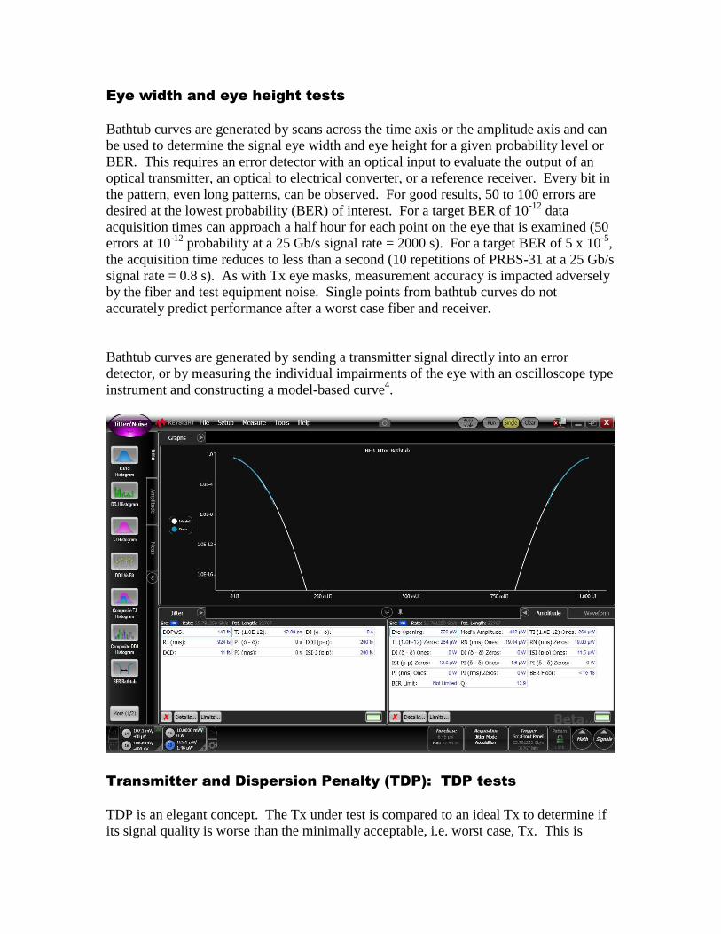
Bathtub curves are generated by scans across the time axis or the amplitude axis and can

be used to determine the signal eye width and eye height for a given probability level or

BER. This requires an error detector with an optical input to evaluate the output of an

optical transmitter, an optical to electrical converter, or a reference receiver. Every bit in

the pattern, even long patterns, can be observed. For good results, 50 to 100 errors are

desired at the lowest probability (BER) of interest. For a target BER of 10-12

data

acquisition times can approach a half hour for each point on the eye that is examined (50

errors at 10-12

probability at a 25 Gb/s signal rate = 2000 s). For a target BER of 5 x 10-5

,

the acquisition time reduces to less than a second (10 repetitions of PRBS-31 at a 25 Gb/s

signal rate = 0.8 s). As with Tx eye masks, measurement accuracy is impacted adversely

by the fiber and test equipment noise. Single points from bathtub curves do not

accurately predict performance after a worst case fiber and receiver.

Bathtub curves are generated by sending a transmitter signal directly into an error

detector, or by measuring the individual impairments of the eye with an oscilloscope type

instrument and constructing a model-based curve4.

Transmitter and Dispersion Penalty (TDP): TDP tests

TDP is an elegant concept. The Tx under test is compared to an ideal Tx to determine if

its signal quality is worse than the minimally acceptable, i.e. worst case, Tx. This is

accomplished by measuring the sensitivity of a Ref Rx using the ideal Tx through a short

fiber and then repeating the Ref Rx sensitivity measurement this time with the Tx DUT

and a worst case fiber. The difference in sensitivity is the TDP result and if it is less than

the maximum permitted the Tx DUT is acceptable. The maximum TDP limit is

determined by accounting for the accumulation of all the losses and penalties for the

worst case Tx and fiber. This accounting can be estimated by a link model, or the TDP

limit can be set by other means as long as the receiver specification is consistent with it.

The correlation between TDP measurement results and combined transmitter

impairments, channel losses and penalties is sufficient to permit a tradeoff between TDP

margin and min OMA (there is a one-to-one tradeoff between Tx output OMA and

margin to the TDP result). This is an attractive feature.

TDP as described above requires an ideal Tx and a worst case fiber. While an ideal Tx is

unlikely, a reference Tx can be used if its impairments can be quantified, i.e. if its TDP is

known. Then, for a Tx DUT to be acceptable its TDP is compared to the TDP max less

the TDP of the Ref Tx. A worst case Tx could serve as the Ref Tx; all Tx DUTs would

just have to be slightly better. Since TDP is a comparative sensitivity test, it is not very

sensitive to test equipment noise.

With TDP, every bit in the test pattern contributes to the result. An error detector is

needed, connected to the output of the optical Ref Rx.

Unfortunately for MMF, a worst case fiber is not available, so a filter defined to provide

the same bandwidth as a worst case fiber is used with a short fiber. This converts some

noise penalties into bandwidth penalties. Tx spectral characteristics and associated

impairments are not captured in the test and TDP value but can be and included in the

triple tradeoff with OMA. Alternatively, a triple trade-off among OMA, TDP and

spectral width can be established, as for 10GBASE-SR. Hence, while TDP can capture

most transmitter attributes and interactions between the Tx and fiber for SMF cases, it is

not as comprehensive for MM cases.

While TDP satisfies the need to quantify the transmitter signal quality, it has some

downsides. It requires a test system including a bit error ratio tester (BERT), a reference

transmitter, and a reference receiver, the combination being expensive as well as difficult

to calibrate. TDP is also a time consuming test, in that BER measurements require

observation of many bits. Cost and test time combine to make TDP impractical in a

manufacturing environment. Thus an alternative test method is desirable.

Transmitter and Dispersion Eye Closure, TDEC, tests

Transmitter and dispersion eye closure (TDEC) is a measure of an optical transmitter’s

vertical eye closure as if observed at the end of a worst case fiber. It is based upon

vertical histogram data from an eye diagram measured through an optical to electrical

converter (O/E) with a bandwidth equivalent to a combined Ref RX and worst case

optical channel. As with Tx eye masks and bathtub curves, eye width and height

measurements and TDP for MMF, the absence of a worst case fiber leads to

compromises. As with TDP, a filter is used to approximate the effect of the worst case

fiber with a worst case Tx; all transmitters are assumed to have worst case wavelength

and spectral characteristics. Instead of a BERT-based Ref Rx the TDEC measurement

can use an oscilloscope with an optical input as the Ref Rx by using an eye closure metric

instead of a Rx sensitivity metric.

The oscilloscope is set up to accumulate samples of the optical eye diagram for the

transmitter under test, as illustrated below. The standard deviation of the noise of the

O/E and oscilloscope combination, S, is determined with no optical input signal and the

same settings as used to capture the histograms described below. The average optical

power (Pave), the crossing points of the eye diagram, and the four vertical histograms

used to calculate TDEC, are all measured using the same test pattern. The 0 UI and 1 UI

crossing points are determined by the average of the eye diagram crossing times, as

measured at Pave, as illustrated below. Four vertical histograms are measured through

the eye diagram, centered at 0.4 UI and 0.6 UI, and above and below Pave, as illustrated.

Mathematical processing of the histograms to derive the TDEC

value

The histograms are analyzed in pairs (early and late) to find the largest amount of

Gaussian noise that could be added to the signal while achieving the target BER. This

amount is adjusted for the known instrument noise in the measurement that would be

different in a link, and effects in a worst case link that are not present in the

measurement. Also, the largest amount of Gaussian noise that could be added to an ideal

signal with the same OMA, for the same BER, is calculated. The ratio of the two noises

is converted into a penalty. The process is described in more detail below:

The largest amount of Gaussian noise that could be added to the signal could be found as

follows:

1. Choose a trial amount of noise. The noise is assumed to have a Gaussian

distribution; this is a reasonable assumption both for an optical receiver and for an

oscilloscope with an optical input.

2. Convolve each histogram with a Gaussian distribution representing this noise,

giving histograms that might be seen in a noisy receiver. The tail of each histogram that

falls on the wrong side of the decision level, which is Pave, gives the BER of that

histogram for that noise.

3. The receiver’s decision timing might be consistently early or late, and typically

half the transmitted bits are ones and half are zeros, so after normalizing each histogram

to a total of 1, take the average of the area under the tails of the upper and lower

histograms on the left, and of the pair on the right. The worst of left and right is the

predicted BER for the transmitter under test, for the trial amount of noise.

4. Compare this BER with the target BER. If it is higher than the target, choose a

new smaller trial amount of noise, if lower, choose higher.

5. Repeat the process until the BER is close to the target. Now we know the largest

amount of Gaussian noise that could be added. In a later section, the adjustments and

subsequent calculation of TDEC are described. But next, an equivalent method of

finding the largest amount of Gaussian noise that could be added, which is described in

IEEE 802.3bm6, is presented.

The calculation can be done without convolutions by the following method, because the

integral of a Gaussian distribution (the Normal curve) is a well-known function, called Q

below, which is related to the “complementary error function”:

Q(x) = ∫x∞ exp(–z

2 / 2) / √(2π) dz

where x is (y – Pave)/σG or (Pave – y)/σG and σG is the left or right standard deviation, σL or

σR.

The two (upper and lower) functions Q can be used as weighting functions. Trial noises

σL and σR are chosen. Each histogram is normalized to 1 and multiplied by a weighting

function Q, which is large for samples near to the decision level Pave (near the middle of

the eye) and small for samples far away. Note that samples from a range of levels

contribute to errors – finding a single point on a histogram would not accurately predict

the BER. The weighted distributions are integrated to obtain the predicted BERs from

upper and lower, left and right, histograms. The left pair of BERs and the right pair are

averaged. New trial noises σL and σR are chosen, and the iteration continues until the

predicted BERs are close to the target. This procedure finds values of σG (σL or σR) such

that the equation below is satisfied:

( ∫ fu(y) Q((y – Pave)/σG)dy / ∫ fu(y) dy + ∫ fl(y) Q((Pave – y)/σG)dy / ∫ fl(y) dy) / 2 = 5 × 10-5

where fu and fl are the upper and lower distributions and σG is the left or right standard

deviation, σL or σR. 5 × 10-5

is the target BER.

The lesser of σL and σR is N.

Now that we have the largest amount of Gaussian noise that could be added to the signal

while achieving the target BER, we adjust this amount. We know how much noise is

contributed by the O/E and oscilloscope combination, so we RSS-add S to the noise N we

have found. We can estimate the modal noise that could be added by the worst optical

channel, by extrapolating from the 10 Gigabit Ethernet link model, so we RSS-subtract

M2. We use a simplification of the formula for mode partition noise in the 10 Gigabit

Ethernet link model to adjust the result by a factor (1-M1).

The result is the noise that could be added by a receiver:

R = (1 – M1)√(N2 + S

2 – M2

2)

where M1 = 0.04 and M2 = 0.0175Pave account for the mode partition noise and modal

noise that could be added by the optical channel, and S is the standard deviation of the

noise of the O/E and oscilloscope combination.

Now we calculate the largest amount of Gaussian noise that could be added to an ideal

signal with the same OMA, which is simply OMA / (2×3.8906), where the factor 3.8906

is chosen because

∫3.8906∞ exp(–z

2 / 2)/√(2π) dz = 5 × 10

-5 which is the BER limit in this case.

TDEC is a penalty (more is worse) given by the ratio of the noise a receiver could add to

an ideal signal to the noise a receiver could add after the transmitter under test and a

worst case channel. Expressed in decibels, this is:

TDEC = 10log10(OMA / (2×3.8906R) ) dB

Determining the maximum allowable TDEC value

The following figure provides a summary of the signal budget for an optical link and

penalties. The total signal budget is just the difference between the minimum Tx output

OMA and the maximum receiver sensitivity and is usually expressed in dB. As shown in

the figure for TDEC all the optical losses and penalties with the exception of channel

insertion loss, IL, combine to yield TDEC.

The difference between Rx sensitivity, RxS OMA and Ref RxS OMA is the portion of

the signal budget allocated for Rx impairments, e.g. bandwidth less than that of the Ref

Rx as well as baseline wander and contributed deterministic jitter. Power penalties are

discussed in detail in references 1 and 7 and just briefly listed here:

Pmn: modal noise penalty due to partial coupling of optical mode groups across

fiber discontinuities

Pmpn: mode partition noise penalty due to variations in power distribution within

mode groups

Prin: RIN penalty due to the intensity related noise of the optical source

Pisi: inter-symbol interference penalty due to transition times extending beyond a

single bit period.

Pcross:, cross product penalty is an adjustment to the sum of the other penalties

to account for the multiplicative effect

In the above figure, the values for Prin*, Pcross* and Pisi* differ from Prin, Pcross and

Pisi, respectively, due to the difference in bandwidth between the worst case Tx and the

Ref Rx. For TDEC, the Ref Rx is assumed to exhibit insignificant base line wander and

generate insignificant deterministic jitter, while the worst case Rx is assumed to have

lower bandwidth than the Ref Rx, exhibit base line wander and contribute deterministic

jitter. This results in an allocation of a measure of the signal power budget to Rx

impairments.

The maximum TDEC limit is determined by accounting for the accumulation of all the

losses and penalties for the worst case Tx and fiber. As with TDP, there is no confidence

in the availability of a worst case fiber. Here a filter is used to yield the same channel

(Tx, medium, Ref Rx) bandwidth as the worst case combination. This accounting can be

estimated by a link model (See above figure). The correlation between TDEC

measurement results and combined transmitter impairments, channel losses and penalties

and channel losses and penalties is sufficient to permit a tradeoff between TDEC margin

and min OMA (there is a one-to-one tradeoff between Tx output OMA and margin to the

TDEC result). This is an attractive feature.

Unlike TDP, modal noise (partial mode coupling in the cable plant), Pmn, and mode

partition noise, Pmpn, are accounted for in the TDEC measurement as noise terms so

there is less compromise in the TDEC margin – OMA tradeoff as seen with the TDP

tradeoff.

Stressed Receiver Sensitivity

TDEC is a metric that provides a means to quantify the signal impairment of an optical

signal. Since it is oscilloscope based, the method can also be used with minor

adjustments to observe and calibrate of a signal when a stressed signal is desired as an

input condition for testing receivers. Consequently, the stressed eye set-up to test

receivers should more closely resemble eyes delivered from worst case transmitters over

a worst case fiber cable plant.

The Ethernet project P802.3bm has adopted it for this purpose. To distinguish it in this

role from its TDEC role, it is renamed Stressed Eye Closure, SEC. Here the TDEC filter

is not used in the Ref Rx and allocations for Pmn and Pmpn are set to zero. Stressed

receiver sensitivity conditions are discussed in detail in reference 6.

Practical considerations for acquiring data for TDEC

measurements

The Digital Communications Analyzer (DCA) is configured to have the 12.6 GHz

bandwidth following a fourth order Bessel Thomson response. The eye diagram is

observed through a simple autoscale function and the crossing points are located to define

the 0 and 1.0 UI positions of the transmitter eye waveform. Histograms of 0.04 UI width,

as described above are placed on the eye diagram:

While all four histograms can be collected with the DCA configured as above, only a

small portion of the total samples available contribute to the data set contained within the

histogram windows. If a large sample population is required, significant sampling

efficiency can be achieved by reducing the time span of the DCA to include only the

regions where the histogram windows are configured.

First the region around the 0.4 UI position is analyzed:

The DCA timespan is then adjusted to include the histograms at the 0.6 UI position:

Practical measurements configured as described above can be achieved in a matter of

seconds.

Example Measurements

The following examples below show TDEC measurement results for two transmitters.

Example 1 has a TDEC value of 2.55 dB, while example 2 has a TDEC value of 3.9 dB.

The eye diagrams, histograms, and associated TDEC parameters are listed, as well as the

resulting TDEC values. Recall that TDEC represents a penalty, and the larger the TDEC

value, the lower the quality of the transmitter. Intuitively this makes sense as the two

examples below show a wider eye opening for the lower TDEC transmitter.

Example 1

TDEC Extraction Example 1

Parameter Units Value

S μW 9.0

Zero μW 262.0

One μW 954.1

Pave μW 615.8

OMA μW 692.1

M1 0.04

M2 μW 10.8

N μW 51.8

R μW 49.4

TDEC dB 2.55

Example 2:

TDEC Extraction Example 2

Parameter Units Value

S μW 9.0

Zero μW 517.8

One μW 1508.6

Pave μW 1021.1

OMA μW 990.8

M1 0.04

M2 μW 17.9

N μW 56.2

R μW 51.9

TDEC dB 3.90

References

1) “Review of the 10Gigabit Ethernet Link Model”, David Cunningham and Piers

Dawe, http://www.avagotech.com/docs/AV02-2485EN

2) Methodologies for Signal Quality Specification. Appendix B (draft 2.2), INCITS

T11 document

3) “Scaling 100G SR4”, John Petrilla, Avago Technologies. Presentation at

INCITS T11 committee

4) “Precision Jitter Analysis Using the Keysight 86100C” Keysight Technologies

Application/Product note, http://literature.cdn.keysight.com/litweb/pdf/5989-

1146EN.pdf).

5) “Eye mask and TDP proposal to replace jitter bathtub”, slide 17, Piers Dawe,

http://ieee802.org/3/ae/public/jan02/dawe_1_0102.pdf

6) IEEE P802.3bm ™ /D3.3 “Draft Standard for Ethernet Amendment: Physical

Layer Specifications and Management Parameters for 40 Gb/s and 100 Gb/s

Operation Over Fiber Optic Cables

7) “Gigabit Ethernet Networking”, D.G. Cunningham and W.G. Lane, Macmillan

Technical Publishing, ISBN 1-57870-062-0