New methods and technologies for regional-scale abundance estimation of land-breeding marine...
14
ORIGINAL PAPER New methods and technologies for regional-scale abundance estimation of land-breeding marine animals: application to Ade ´lie penguin populations in East Antarctica Colin Southwell • John McKinlay • Matt Low • David Wilson • Kym Newbery • Jan L. Lieser • Louise Emmerson Received: 26 October 2012 / Revised: 20 February 2013 / Accepted: 22 February 2013 / Published online: 30 March 2013 Ó Springer-Verlag Berlin Heidelberg 2013 Abstract Land-breeding marine animals such as pen- guins, flying seabirds and pinnipeds are important com- ponents of marine ecosystems, and their abundance has been used extensively as an indication of ecosystem status and change. Until recently, many efforts to measure and monitor abundance of these species’ groups have focussed on smaller populations and spatial scales, and efforts to account for perception bias and availability bias have been variable and often ad hoc. We describe a suite of new methods, technologies and estimation procedures for cost- effective, large-scale abundance estimation within a gen- eral estimation framework and illustrate their application on large Ade ´lie penguin populations in two regions of East Antarctica. The methods include photographic sample counts, automated cameras for collecting availability data, and bootstrap estimation to adjust counts for the sampling fraction, perception bias, and availability bias, and are applicable for a range of land-breeding marine species. The methods will improve our ability to obtain population data over large spatial and population scales within tight logistic, environmental and time constraints. This first application of the methods has given new insights into the biases and uncertainties in abundance estimation for pen- guins and other land-breeding marine species. We provide guidelines for applying the methods in future surveys. Keywords Bootstrap estimation Detection bias Distance sampling Photography Remotely operating cameras Sample designs Introduction Animal species that forage in marine environments but breed on land, such as penguins, flying seabirds and pinnipeds, are important components of marine ecosystems and are often used to indicate marine ecosystem status and change (Montevecchi 1993; Furness and Camphusen 1997; Piatt et al. 2007). They have several advantages as marine indicators over other marine species, including their high visibility, their relative accessibility for study when breeding on land, and their ability to forage widely in the marine environment in search of a range of marine prey (Piatt et al. 2007). These species’ groups can provide insights into marine ecosystem processes at different spa- tial and temporal scales through the measurement of a range of demographic, behavioural and physiological parameters (Reid et al. 2005). The abundance of breeding populations is a frequently measured parameter. Abun- dance reflects the collective outcome of key demographic processes, is relatively easy to measure compared with C. Southwell (&) J. McKinlay M. Low D. Wilson K. Newbery L. Emmerson Australian Antarctic Division, Department of Sustainability, Environment, Water, Population and Communities, 203 Channel Highway, Kingston, TAS 7050, Australia e-mail: [email protected] Present Address: M. Low Department of Ecology, Swedish University of Agricultural Sciences, Uppsala, Sweden Present Address: D. Wilson Ecology and Heritage Partners, 292 Mt Alexander Road, Ascot Vale, VIC 3032, Australia J. L. Lieser Antarctic Climate and Ecosystems Cooperative Research Centre, Centenary Building, Private Bag 80, Hobart, TAS 7001, Australia 123 Polar Biol (2013) 36:843–856 DOI 10.1007/s00300-013-1310-z
-
Upload
kym-newbery -
Category
Documents
-
view
213 -
download
0
Transcript of New methods and technologies for regional-scale abundance estimation of land-breeding marine...
ORIGINAL PAPER
New methods and technologies for regional-scale abundanceestimation of land-breeding marine animals: applicationto Adelie penguin populations in East Antarctica
Colin Southwell • John McKinlay • Matt Low •
David Wilson • Kym Newbery • Jan L. Lieser •
Louise Emmerson
Received: 26 October 2012 / Revised: 20 February 2013 / Accepted: 22 February 2013 / Published online: 30 March 2013
� Springer-Verlag Berlin Heidelberg 2013
Abstract Land-breeding marine animals such as pen-
guins, flying seabirds and pinnipeds are important com-
ponents of marine ecosystems, and their abundance has
been used extensively as an indication of ecosystem status
and change. Until recently, many efforts to measure and
monitor abundance of these species’ groups have focussed
on smaller populations and spatial scales, and efforts to
account for perception bias and availability bias have been
variable and often ad hoc. We describe a suite of new
methods, technologies and estimation procedures for cost-
effective, large-scale abundance estimation within a gen-
eral estimation framework and illustrate their application
on large Adelie penguin populations in two regions of East
Antarctica. The methods include photographic sample
counts, automated cameras for collecting availability data,
and bootstrap estimation to adjust counts for the sampling
fraction, perception bias, and availability bias, and are
applicable for a range of land-breeding marine species. The
methods will improve our ability to obtain population data
over large spatial and population scales within tight
logistic, environmental and time constraints. This first
application of the methods has given new insights into the
biases and uncertainties in abundance estimation for pen-
guins and other land-breeding marine species. We provide
guidelines for applying the methods in future surveys.
Keywords Bootstrap estimation � Detection bias �Distance sampling � Photography � Remotely operating
cameras � Sample designs
Introduction
Animal species that forage in marine environments but
breed on land, such as penguins, flying seabirds and
pinnipeds, are important components of marine ecosystems
and are often used to indicate marine ecosystem status and
change (Montevecchi 1993; Furness and Camphusen 1997;
Piatt et al. 2007). They have several advantages as marine
indicators over other marine species, including their high
visibility, their relative accessibility for study when
breeding on land, and their ability to forage widely in the
marine environment in search of a range of marine prey
(Piatt et al. 2007). These species’ groups can provide
insights into marine ecosystem processes at different spa-
tial and temporal scales through the measurement of a
range of demographic, behavioural and physiological
parameters (Reid et al. 2005). The abundance of breeding
populations is a frequently measured parameter. Abun-
dance reflects the collective outcome of key demographic
processes, is relatively easy to measure compared with
C. Southwell (&) � J. McKinlay � M. Low � D. Wilson �K. Newbery � L. Emmerson
Australian Antarctic Division, Department of Sustainability,
Environment, Water, Population and Communities,
203 Channel Highway, Kingston, TAS 7050, Australia
e-mail: [email protected]
Present Address:M. Low
Department of Ecology, Swedish University of Agricultural
Sciences, Uppsala, Sweden
Present Address:D. Wilson
Ecology and Heritage Partners, 292 Mt Alexander Road,
Ascot Vale, VIC 3032, Australia
J. L. Lieser
Antarctic Climate and Ecosystems Cooperative Research Centre,
Centenary Building, Private Bag 80, Hobart, TAS 7001,
Australia
123
Polar Biol (2013) 36:843–856
DOI 10.1007/s00300-013-1310-z
other demographic parameters (Thompson et al. 1998), is a
primary determinant of biomass which is a key input
parameter for marine ecosystem models (Pauly et al. 2000),
and can reflect ecosystem processes over large spatial and
temporal scales (Reid et al. 2005).
The development of robust methods for estimating
animal abundance is an important and rich area of research
that serves as a foundation for many ecological and man-
agement studies. Over the past three decades, much work
has focussed on developing techniques to estimate the
unknown fraction of animals that are not detected in
abundance surveys because of perception bias and avail-
ability bias (Pollock et al. 2004). A recent emerging area of
methodological research is the development of cost-effec-
tive abundance estimation methods for large-scale infer-
ence, given the scale of human-induced impact on
ecosystems is increasing and agencies need to manage over
large scales but operate within tight logistic and financial
constraints (Pollock et al. 2002; Field et al. 2005; Jones
2011). While research on incomplete detection and cost-
effective methods for large-scale inference has spawned
many abundance estimation techniques for a range of
species, they can all be considered within a general abun-
dance estimation framework (Borchers et al. 2002; Wil-
liams et al. 2002; Pollock et al. 2004). The advantages of a
general framework are that it simplifies apparently com-
plex and unique problems to a small set of common issues,
encourages researchers to consider all components of
estimation, and provides a basis for rigorous statistical
estimation.
These developments in the general field of animal
abundance estimation are particularly relevant to land-
breeding marine animals and their use as marine indicators.
Penguins are a key species group in Southern Ocean eco-
systems and their abundance has been used extensively as
an indication of ecosystem status and change (CCAMLR
2004; Jenouvrier et al. 2006; Trivelpiece et al. 2011; Lynch
et al. 2012). However, until recently, many efforts to
measure and monitor the abundance of penguin popula-
tions have focussed on smaller population and spatial
scales, and efforts to account for perception bias and
availability bias have been variable and often ad hoc. This
situation is now changing as researchers strive to estimate
penguin populations over larger population and spatial
scales in recognition of the increasing scale of human-
induced impacts such as fisheries and climate change
(Lynch et al. 2012; Trathan et al. 2012) and to improve the
comparability and reliability of abundance estimates by
developing rigorous statistical methods for estimating and
accounting for detection bias (Lynch et al. 2009; McKinlay
et al. 2010; Southwell et al. 2010; Trathan et al. 2012).
In this paper, we build on these recent developments by
describing the application of an integrated suite of
methods, technologies and estimation procedures for cost-
effective, large-scale abundance estimation of Adelie
penguin populations (Pygoscelis adeliae) within the Pol-
lock et al. (2004) general framework. Although we illus-
trate the methods through application to Adelie penguin
populations, they have relevance and potential application
for a range of land-breeding marine species in polar
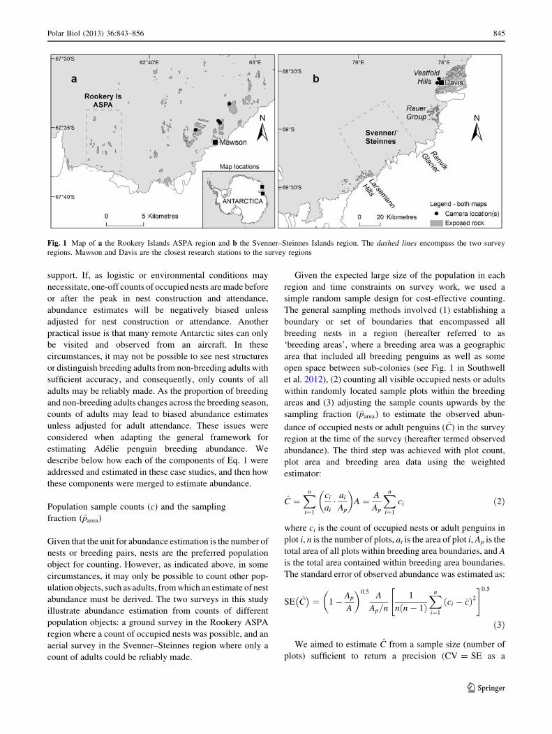
regions. We do this in two regions of East Antarctica with
large Adelie penguin breeding populations: the Rookery
Islands Antarctic Specially Protected Area (hereafter
referred to as the Rookery ASPA region, Fig. 1) off the
Mac.Robertson Land coast, and the Svenner and Steinnes
Islands between the Larsemann Hills and Ranvik Glacier of
the Ingrid Christensen Coast (hereafter referred to as the
Svenner–Steinnes region, Fig. 1). The two regional surveys
illustrate how the general framework and methods can
achieve standardised estimation at large population scales
from counts of different population objects that are subject
to differing degrees of perception and availability bias.
Methods
General estimation framework
In the general framework proposed by Pollock et al. (2004),
the abundance of population objects in a survey region (N)
can be estimated by obtaining a count (c) of objects and
adjusting this count upwards according to (1) the fraction of
the survey region that is sampled (parea), (2) the fraction of
population objects available to be counted (availability bias,
pa) and (3) the fraction of population objects detected given
availability (perception bias, pda), that is,
N ¼ c
parea:pa:pda
ð1Þ
The abundance of penguins and flying seabirds is
generally estimated from counts of population objects (e.g.
adults, nests or chicks) at their breeding sites, and the
commonly accepted unit for estimating abundance,
including Adelie penguins, is the number of nests or
breeding pairs. For Adelie penguins, an optimal time to
estimate the number of breeding pairs is near the end of egg
laying (CCAMLR 2004) when few pairs have failed their
breeding attempt and the number of occupied nests is at or
close to its maximum. At this stage, most breeding females
and non-breeding penguins have left the breeding site and the
population remaining at the site is comprised almost entirely
of single adult males on their nests incubating eggs.
However, one of the practical difficulties in estimating the
abundance of Adelie penguin breeding pairs is that it is often
impossible to visit breeding sites at an optimal time due to
unpredictable weather and ice conditions and limited logistic
844 Polar Biol (2013) 36:843–856
123
support. If, as logistic or environmental conditions may
necessitate, one-off counts of occupied nests are made before
or after the peak in nest construction and attendance,
abundance estimates will be negatively biased unless
adjusted for nest construction or attendance. Another
practical issue is that many remote Antarctic sites can only
be visited and observed from an aircraft. In these
circumstances, it may not be possible to see nest structures
or distinguish breeding adults from non-breeding adults with
sufficient accuracy, and consequently, only counts of all
adults may be reliably made. As the proportion of breeding
and non-breeding adults changes across the breeding season,
counts of adults may lead to biased abundance estimates
unless adjusted for adult attendance. These issues were
considered when adapting the general framework for
estimating Adelie penguin breeding abundance. We
describe below how each of the components of Eq. 1 were
addressed and estimated in these case studies, and then how
these components were merged to estimate abundance.
Population sample counts (c) and the sampling
fraction (parea)
Given that the unit for abundance estimation is the number of
nests or breeding pairs, nests are the preferred population
object for counting. However, as indicated above, in some
circumstances, it may only be possible to count other pop-
ulation objects, such as adults, from which an estimate of nest
abundance must be derived. The two surveys in this study
illustrate abundance estimation from counts of different
population objects: a ground survey in the Rookery ASPA
region where a count of occupied nests was possible, and an
aerial survey in the Svenner–Steinnes region where only a
count of adults could be reliably made.
Given the expected large size of the population in each
region and time constraints on survey work, we used a
simple random sample design for cost-effective counting.
The general sampling methods involved (1) establishing a
boundary or set of boundaries that encompassed all
breeding nests in a region (hereafter referred to as
‘breeding areas’, where a breeding area was a geographic
area that included all breeding penguins as well as some
open space between sub-colonies (see Fig. 1 in Southwell
et al. 2012), (2) counting all visible occupied nests or adults
within randomly located sample plots within the breeding
areas and (3) adjusting the sample counts upwards by the
sampling fraction (parea) to estimate the observed abun-
dance of occupied nests or adult penguins (C) in the survey
region at the time of the survey (hereafter termed observed
abundance). The third step was achieved with plot count,
plot area and breeding area data using the weighted
estimator:
C ¼Xn
i¼1
ci
ai� ai
Ap
� �A ¼ A
Ap
Xn
i¼1
ci ð2Þ
where ci is the count of occupied nests or adult penguins in
plot i, n is the number of plots, ai is the area of plot i, Ap is the
total area of all plots within breeding area boundaries, and A
is the total area contained within breeding area boundaries.
The standard error of observed abundance was estimated as:
SE C� �¼ 1� Ap
A
� �0:5A
Ap=n
1
n n� 1ð ÞXn
i¼1
ci � �cð Þ2" #0:5
ð3Þ
We aimed to estimate C from a sample size (number of
plots) sufficient to return a precision (CV = SE as a
Fig. 1 Map of a the Rookery Islands ASPA region and b the Svenner–Steinnes Islands region. The dashed lines encompass the two survey
regions. Mawson and Davis are the closest research stations to the survey regions
Polar Biol (2013) 36:843–856 845
123
percent of the mean) of 10 % for observed abundance in
each region.
The detailed survey-specific methods for the ground-
based sample survey in the Rookery ASPA region were as
follows. We mapped the boundaries of all breeding areas
by walking around groups of sub-colonies with a hand-held
Garmin Etrex GPS set to log locations at 5-s intervals.
While walking these boundaries, we remained within
5–20 m from sub-colony perimeters, and within these
distance constraints, attempted to minimise the boundary
length encompassing groups of sub-colonies. Simulation
studies (Southwell et al. 2012) showed that this strategy of
‘coarse’ boundary mapping was more efficient than ‘exact’
mapping of sub-colony boundaries. We then converted the
GPS-defined boundaries into a set of GIS polygons, used
the GIS survey tool developed by Southwell et al. (2012)
for planning and evaluating sample survey designs to
generate locations and boundaries of sample plots across
the entire survey region and selected 320 plots (the sample
size predicted from a pilot study to return a 10 % CV) that
completely or partially overlapped with breeding areas for
sample counts. Each sample plot consisted of two 4 9 5 m
sub-plots facing in opposite directions and offset by 2 m
from a central location. To locate plots in the field, we
imported their central locations, obtained as output from
the GIS survey planning tool, into a GPS and used the GPS
to navigate to each location. At each sample plot, we used a
camera mounted on top of a 3-m pole to take oblique
photographs of the area covered by the two sub-plots sur-
rounding the central point (Fig. 1 in Low et al. 2008). This
was done by placing the camera-pole at the central point,
holding it vertically using a spirit level, and taking a
photograph in each of the two directions at 180� to each
other. To avoid bias in the areas photographed, we used
predetermined rules for the direction of the camera: (1) for
flat ground, photographs were taken in magnetic north and
south directions, and (2) for sloping ground, photographs
were taken directly up-slope and down-slope. We used
upslope–downslope photographs because this allowed us to
correct for distortions in perspective with greater accuracy
than would have been possible for cross-slope photographs.
To make these corrections, we also recorded the slope of
the ground in each sub-plot in a 5-point category scale [flat
(0�–3�), moderate up (4�–10�), moderate down (4�–10�),
steep up ([10�) and steep down ([10�)]. To minimise time
in the field and disturbance to penguins, sub-plot counts
were made in the laboratory from the photographs after
digitally overlaying slope-specific templates to delineate
‘virtual’ sub-plot boundaries. Low et al. (2008) showed that
delineating plots in this way resulted in only minor errors
(*2–3 %) in classifying penguins as inside or outside the
plots, provided slopes were not too steep (\17�). We
counted the number of occupied nests in each sub-plot and
summed sub-plot counts to obtain a total count of occupied
nests for each plot (ci). Values for ai, Ap and A in Eqs. 2
and 3 were obtained from shapefiles produced by the sur-
vey planning tool, which along with values for ci and n
(320) were used to estimate the observed abundance of
occupied nests and its standard error.
The detailed survey-specific methods for the aerial-
based sample survey in the Svenner–Steinnes region were
as follows. We mapped the boundaries of all breeding
areas in the survey region from aerial photographs of the
breeding sites. Photographs were taken from an AS350BA
Squirrel helicopter flying at 80 knots speed and 750 m
altitude. The helicopter carried a downward-looking Has-
selblad H3DII-50 camera fitted with a 150 mm lens. This
set-up resulted in ground coverage of 245 m by 184 m for
each photograph. A 3-s interval between photographs
ensured that consecutive photographs overlapped along a
flight line, and a flight line spacing of 200 m ensured that
photographs overlapped between flight lines. We aimed to
achieve complete photographic coverage of each breeding
site. The camera auto-focussed effectively at infinity using
the software Phocus and used a shutter speed of 1/800th s.
Following the survey flight, groups of 3–4 photographs
taken along a flight line within a breeding site were stit-
ched together using the software Microsoft Image Com-
posite Editor. These mosaics were then geo-referenced
against shapefiles of the coastline in a GIS so that a
complete photo-mosaic of each breeding site could be
viewed. We then imported the geo-referenced photo-
mosaics into a GIS and drew polygon boundaries around
sub-colonies or groups of sub-colonies to delineate all
breeding areas in the region. The boundaries had a buffer
of 1–5 m from the outermost penguins. The GIS survey
planning tool was then used to generate a shapefile with a
grid of 10 9 10 m plots across the entire sub-region and
to then generate a second shapefile that contained only the
parts of those plots that overlapped with the breeding
areas. We then randomly selected 90 plots (the sample
size predicted from a pilot study to return a 10 % CV) and
counted the number of adult penguins (both lying and
standing) within each selected plot. We chose to count all
penguins rather than just penguins on nests because we
were not confident in distinguishing penguins on nests
from penguins off nests. The plot counts were then scaled
up by the sampling fraction in the same way as for the
ground survey to estimate the observed number of adult
penguins present in all the breeding areas at the time of
the survey.
Estimating the availability fraction (pa)
The term availability refers to counting bias resulting from
population objects that are present but completely obscured
846 Polar Biol (2013) 36:843–856
123
from view and hence not available for counting (Pollock
et al. 2004). In this classic sense, the availability fraction is
always B1. This concept can be extended to surveys of
land-breeding marine species, such as Adelie penguins,
where some breeding adults may forage away from the
breeding site during the breeding season to provision their
chicks, or some nests that were occupied early in the
breeding season may be abandoned at a later time if the
eggs fail to hatch or the chicks die, and hence, population
objects such as breeding adults or occupied nests may not
always be available for counting at the breeding site. There
are also times during the breeding season when the pres-
ence of non-breeders at the breeding site results in a pop-
ulation of adult penguins that is greater than the number of
breeding adults or breeding pairs, and hence, the avail-
ability fraction can be[1 for counts of adults. In this study,
we have interpreted the concept of availability in its
broadest sense when applying it to Adelie penguins by
having no upper bound to pa.
We applied new remote camera technology to collect
availability data and new analysis methods to estimate
availability fractions. Remotely operating cameras (New-
bery and Southwell 2009) were established at several
Adelie penguin breeding sites close to the two survey
regions prior to the ground and aerial surveys (nine
cameras on four islands near Mawson station 15 km east
of the Rookery ASPA region; five cameras on two islands
near Davis station 60 km east of the Svenner–Steinnes
region). The cameras were established adjacent to breed-
ing sub-colonies and overlooked areas covering 30–50
nests. Once established, each camera took a single pho-
tograph at solar midday each day. We counted the number
of adults and occupied nests in a fixed region of each daily
photograph and then standardised the time series counts of
adults and occupied nests against a count of occupied
nests at the stage in the breeding phenology recommended
in the Standard Methods of the CCAMLR Ecosystem
Monitoring Program for penguin population counts
(1 week after peak egg laying, Method A3 in CCAMLR
2004). At this stage, the population at the breeding site
comprises mostly adult males incubating eggs on nests,
and the number of occupied nests is at or close to its
maximum. The peak in egg laying can be difficult to
determine through observation of eggs in the photographs.
However, since females leave the breeding site shortly
after laying their second egg, we used the maximum rate
of decline in adult numbers after the initial peak in arrival
as a proxy for the peak in egg laying (Southwell et al.
2010). The standardised time series counts of adults and
occupied nests were then modelled using a generalised
additive model (GAM), and the modelled time series were
used to generate object- and stage-specific factors to adjust
sample counts (see below).
Estimating the detection fraction given availability (pda)
Counts of animals are often negatively biased because
some are not detected even though they are present and
potentially visible in the area searched (perception bias,
Pollock et al. 2004). Consistent with this generalisation,
experimental work using model penguins (Low et al. 2008)
showed that sample plot counts using the pole-mounted
camera may be slightly negatively biased as a result of the
camera’s oblique view and fixed position. In the case of
counting penguins from aerial photographs, counts could
also be positively biased if objects such as rocks or shad-
ows are mistaken for penguins. Thus, estimates of observed
abundance from both the ground and aerial sample surveys
may have been biased in relation to true abundance as a
result of perception bias. We used different methods to
assess perception bias for the two surveys.
For the ground survey, we used distance sampling to
estimate the probability of detecting occupied nests that
were present in the sample plots. Each of the sub-plot
boundary templates was divided in 5 equal-width 1-m bins
and counts of occupied nests were made within each bin.
We then used DISTANCE 5.0 software (Thomas et al.
2006) to estimate detection probability from the bin count
data. Four candidate detection functions were considered
(uniform ? cosine; uniform ? simple-polynomial; half-
normal ? hermite-polynomial; and half-normal ? cosine),
and the best model was selected on the basis of AIC values.
For the aerial survey, we assessed how similar counts
from aerial photographs were to counts made directly by
observers on the ground at 14 small- to medium-sized sub-
colonies (B300 penguins) situated on four islands off the
Vestfold Hills close to where the remotely operating
cameras were located. The work was undertaken on the
same day as the regional aerial survey. Ground counts of
all penguins in each of the 14 sub-colonies were carried out
by two observers counting independently, and the average
of their counts was taken as the ‘best’ count. Aerial pho-
tographs of the same sub-colonies were taken within 3 h of
the ground counts using the same survey and photographic
settings as for the regional survey, and counts were made
from the photographs by the same observer who counted
the survey photographs. Ground and aerial counts of the
sub-colonies were then compared using a paired t test.
Combining the estimation components
This was achieved using a parametric bootstrap imple-
mentation using the software ICESCAPE (McKinlay et al.
2010). The procedure uses the estimates of observed
abundance and detectability, and availability time series
data, to generate a distribution of estimates of the number
of occupied nests at the standardised stage of the breeding
Polar Biol (2013) 36:843–856 847
123
phenology, and in these applications operated as follows:
(1) a distribution of observed abundance estimates for
occupied nests or adults was generated by drawing 1,000
replicates from a normal distribution defined by the
observed abundance estimate and its standard error; (2) a
distribution of availability adjustment fractions was
obtained by (i) drawing 1,000 dates from a uniform dis-
tribution defined by the date-range over which the survey
took place, (ii) randomly selecting a date and an avail-
ability curve from the pool of curves (nine curves for the
Rookery ASPA region and five for the Svenner–Steinnes
region), (iii) drawing an availability fraction replicate from
a normal distribution with mean equal to the predicted
value for that date and standard deviation equal to the
standard error of the fitted GAM function at that point, and
(iv) repeating this process to generate 1,000 availability
fraction replicates; (3) a distribution of detection fractions
was generated by drawing 1,000 replicates from a normal
distribution defined by the detection probability estimate
and its standard error (obtained from DISTANCE for the
Rookery ASPA region and from the air-ground comparison
counts for the Svenner–Steinnes region); (4) having gen-
erated distributions for observed abundance, availability
and detectability, a distribution of 1,000 final adjusted
occupied nest estimates for the standardised stage of the
breeding phenology was obtained by iteratively calculating
the product of an observed abundance replicate, the inverse
of an availability fraction replicate and the inverse of a
detection fraction replicate; and (5) the distribution of final
adjusted estimates was summarised by the median and
95 % confidence interval, where a 100.(1 - a) % confi-
dence interval is taken as the a/2 and 1 - a/2 percentile
points.
Uncertainty
We explored options for reducing or minimising uncer-
tainty in future surveys that use the new methods by sim-
ulating abundance estimates obtained in different years,
over different date-ranges and with different sample sizes
(number of sample plots) with data obtained from the
Rookery ASPA region. First, we assumed that the same
estimates of observed abundance and detectability were
obtained over the same date-range as the Rookery ASPA
survey, but used availability data from the region in the
four subsequent breeding seasons (i.e. from 2008–2009 to
2011–2012) to obtain a distribution of 1,000 simulated final
adjusted abundance estimates for these seasons. Second,
we assumed that the same estimates of observed abundance
and detectability were obtained within a shorter, earlier
date-range (23–25 November) and used availability data
for this date-range from the five breeding seasons
2007–2008 to 2011–2012 to obtain distributions of simu-
lated final adjusted abundance estimates for these seasons.
Finally, we simulated final adjusted abundance estimates
for the five seasons and two date-ranges assuming that the
sampling error in estimating observed abundance was
successively reduced from a CV of 10 % through to 0 %
(the latter inferring a census or complete count) by
increasing the number of sample plots counted. We then
used the distributions of final abundance estimates to
examine uncertainty for the various survey design options.
Results
Rookery ASPA region
We mapped breeding areas in the Rookery ASPA region
over a three-day period at the end of November 2007.
Although sample plot photographs could have also been
completed in a few days, the work extended over a two-
week period from 3–15 December 2007 (Table 1; Fig. 2)
because of unsuitable weather and the need for the survey
team to work on other projects. A total of 2,684 occupied
nests were counted in the 320 sample plots which covered
3.6 % of the mapped breeding areas. Adjusting the sample
count upwards by the sampling fraction gave an observed
abundance estimate (C) of 73,630 (SE = 6,268) occupied
nests at the time of the survey.
Table 1 Survey and estimation details for the Rookery ASPA and Svenner–Steinnes regional abundance surveys
Survey details Rookery ASPA region Svenner–Steinnes
region
Dates when sample plot photographs were taken 3–15 December 2007 20 November 2010
Population object counted Occupied nests Adults
Observed abundance of population objects at the time of the survey (C, SE) 73,630 (6,268) 44,022 (4,583)
Availability fraction (pa: median, 95 % CI) 0.872 (0.411–0.984) 1.713 (1.574–1.923)
Detection fraction given availability (pda: mean, 95 % CI) 0.943 (0.916–0.969) 1.000 (1.000–1.000)
Estimated number of occupied nests 1 week after the peak in egg laying
(N: median, 95 % CI)
90,627 (70,685–197,832) 25,658 (20,092–31,654)
848 Polar Biol (2013) 36:843–856
123
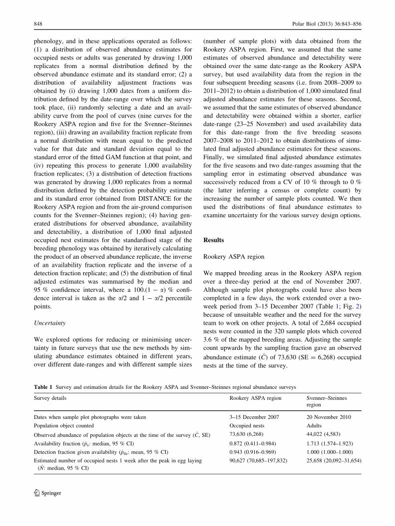
The dates selected for the standardised stage of the
breeding phenology at the nine camera sites ranged from
27–30 November and included the period when the number
of occupied nests was at its maximum (Fig. 2b). There was
a strong decline in the number of occupied nests from
early- to late-December 2007 at three of the nine camera
sites and a small-moderate decline at the other six sites
(Fig. 2b). The strong decline at the three sites commenced
during a 2-day blizzard across the region and occurred at
sites where the microhabitat appeared to offer little shelter.
As a consequence, the standardised counts of occupied
nests from the nine camera sites became increasingly dis-
parate over the 2-week period that sample plot photographs
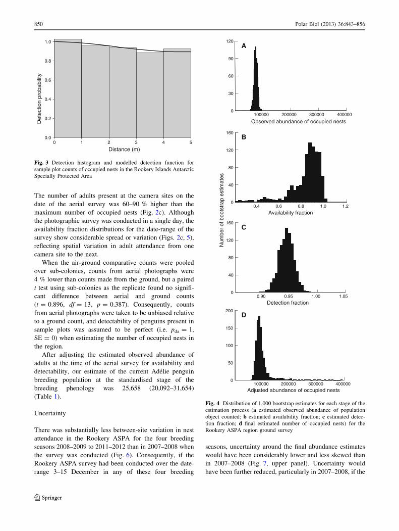
were taken (Fig. 2b). This disparity resulted in a strongly
skewed distribution of availability fractions for the date-
range of the survey period, with a median value of 0.872
and a long tail of low fractions (95 percentile range
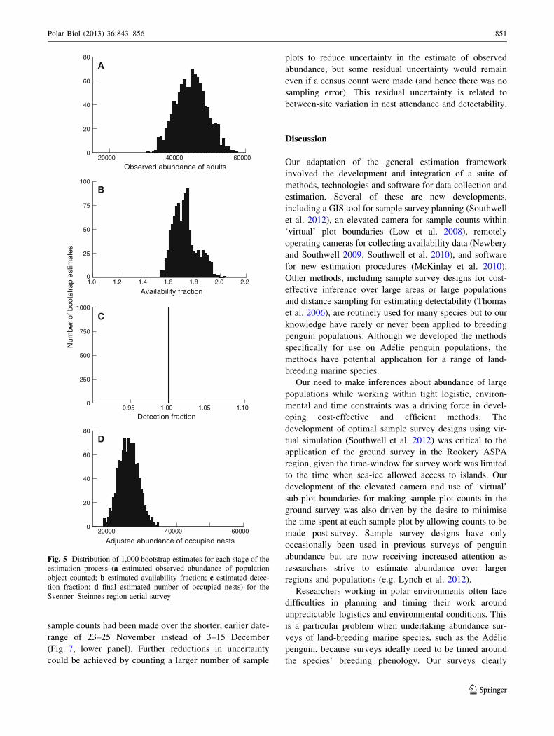
0.411–0.984, Table 1; Fig. 4b).
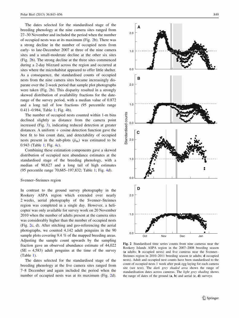
The number of occupied nests counted within 1-m bins
declined slightly as distance from the camera point
increased (Fig. 3), indicating reduced detection at greater
distances. A uniform ? cosine detection function gave the
best fit to bin count data, and detectability of occupied
nests present in the sub-plots (pda) was estimated to be
0.943 (Table 1; Fig. 4c).
Combining these estimation components gave a skewed
distribution of occupied nest abundance estimates at the
standardised stage of the breeding phenology, with a
median of 90,627 and a long tail of high estimates
(95 percentile range 70,685–197,832; Table 1; Fig. 4d).
Svenner–Steinnes region
In contrast to the ground survey photography in the
Rookery ASPA region which extended over nearly
2 weeks, aerial photography of the Svenner–Steinnes
region was completed in a single day. However, a heli-
copter was only available for survey work on 20 November
2010 when the number of adults present at the camera sites
was considerably higher than the number of occupied nests
(Fig. 2c, d). After stitching and geo-referencing the aerial
photographs, we counted 4,142 adult penguins in the 90
sample plots covering 9.4 % of the mapped breeding areas.
Adjusting the sample count upwards by the sampling
fraction gave an observed abundance estimate of 44,022
(SE = 4,583) adult penguins at the time of the survey
(Table 1).
The dates selected for the standardised stage of the
breeding phenology at the five camera sites ranged from
7–8 December and again included the period when the
number of occupied nests was at its maximum (Fig. 2d).
2.0
1.0
0.0
A
2.0
1.0
0.0S
tand
ardi
sed
coun
ts
B
2.0
1.0
0.0
C
2.0
1.0
0.0Oct Nov JanDec
D
Fig. 2 Standardised time series counts from nine cameras near the
Rookery Islands ASPA region in the 2007–2008 breeding season
(a adults; b occupied nests) and five cameras near the Svenner–
Steinnes region in 2010–2011 breeding season (c adults; d occupied
nests). Adult and occupied nest counts have been standardised to the
count of occupied nests 1 week after peak egg laying for each camera
site (see text). The dark grey shaded area shows the range of
standardisation dates across cameras. The light grey shading shows
the range of dates of the ground (a, b) and aerial (c, d) surveys
Polar Biol (2013) 36:843–856 849
123
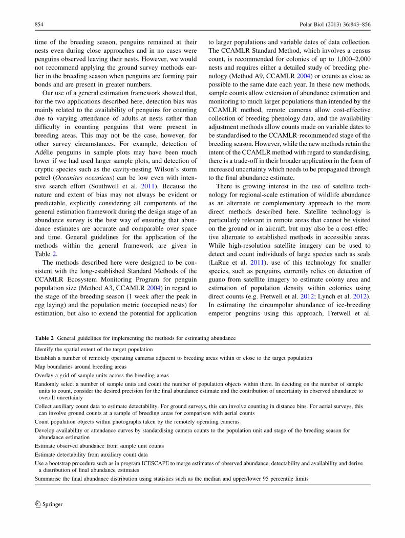
The number of adults present at the camera sites on the
date of the aerial survey was 60–90 % higher than the
maximum number of occupied nests (Fig. 2c). Although
the photographic survey was conducted in a single day, the
availability fraction distributions for the date-range of the
survey show considerable spread or variation (Figs. 2c, 5),
reflecting spatial variation in adult attendance from one
camera site to the next.
When the air-ground comparative counts were pooled
over sub-colonies, counts from aerial photographs were
4 % lower than counts made from the ground, but a paired
t test using sub-colonies as the replicate found no signifi-
cant difference between aerial and ground counts
(t = 0.896, df = 13, p = 0.387). Consequently, counts
from aerial photographs were taken to be unbiased relative
to a ground count, and detectability of penguins present in
sample plots was assumed to be perfect (i.e. pda = 1,
SE = 0) when estimating the number of occupied nests in
the region.
After adjusting the estimated observed abundance of
adults at the time of the aerial survey for availability and
detectability, our estimate of the current Adelie penguin
breeding population at the standardised stage of the
breeding phenology was 25,658 (20,092–31,654)
(Table 1).
Uncertainty
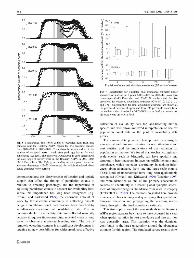
There was substantially less between-site variation in nest
attendance in the Rookery ASPA for the four breeding
seasons 2008–2009 to 2011–2012 than in 2007–2008 when
the survey was conducted (Fig. 6). Consequently, if the
Rookery ASPA survey had been conducted over the date-
range 3–15 December in any of these four breeding
seasons, uncertainty around the final abundance estimates
would have been considerably lower and less skewed than
in 2007–2008 (Fig. 7, upper panel). Uncertainty would
have been further reduced, particularly in 2007–2008, if the
0 1 2 3 4 50.0
0.2
0.4
0.6
0.8
1.0D
etec
tion
prob
abili
ty
Distance (m)
Fig. 3 Detection histogram and modelled detection function for
sample plot counts of occupied nests in the Rookery Islands Antarctic
Specially Protected Area
100000 200000 300000 4000000
30
60
90
120
Observed abundance of occupied nests
0.4 0.6 0.8 1.0 1.20
40
80
120
160
Availability fraction
Num
ber
of b
oots
trap
est
imat
es
0
40
80
120
160
Detection fraction0.90 0.95 1.00 1.05
100000 200000 300000 4000000
50
100
150
200
Adjusted abundance of occupied nests
A
B
C
D
Fig. 4 Distribution of 1,000 bootstrap estimates for each stage of the
estimation process (a estimated observed abundance of population
object counted; b estimated availability fraction; c estimated detec-
tion fraction; d final estimated number of occupied nests) for the
Rookery ASPA region ground survey
850 Polar Biol (2013) 36:843–856
123
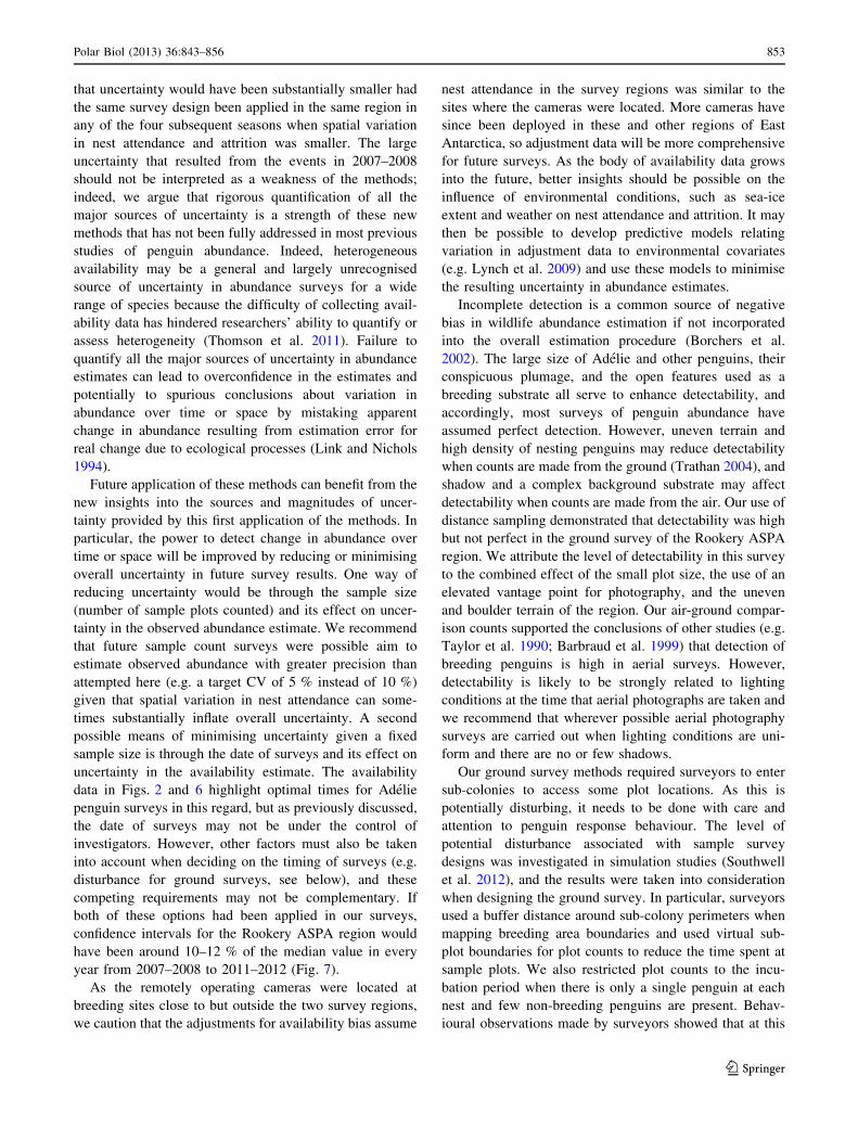
sample counts had been made over the shorter, earlier date-
range of 23–25 November instead of 3–15 December
(Fig. 7, lower panel). Further reductions in uncertainty
could be achieved by counting a larger number of sample
plots to reduce uncertainty in the estimate of observed
abundance, but some residual uncertainty would remain
even if a census count were made (and hence there was no
sampling error). This residual uncertainty is related to
between-site variation in nest attendance and detectability.
Discussion
Our adaptation of the general estimation framework
involved the development and integration of a suite of
methods, technologies and software for data collection and
estimation. Several of these are new developments,
including a GIS tool for sample survey planning (Southwell
et al. 2012), an elevated camera for sample counts within
‘virtual’ plot boundaries (Low et al. 2008), remotely
operating cameras for collecting availability data (Newbery
and Southwell 2009; Southwell et al. 2010), and software
for new estimation procedures (McKinlay et al. 2010).
Other methods, including sample survey designs for cost-
effective inference over large areas or large populations
and distance sampling for estimating detectability (Thomas
et al. 2006), are routinely used for many species but to our
knowledge have rarely or never been applied to breeding
penguin populations. Although we developed the methods
specifically for use on Adelie penguin populations, the
methods have potential application for a range of land-
breeding marine species.
Our need to make inferences about abundance of large
populations while working within tight logistic, environ-
mental and time constraints was a driving force in devel-
oping cost-effective and efficient methods. The
development of optimal sample survey designs using vir-
tual simulation (Southwell et al. 2012) was critical to the
application of the ground survey in the Rookery ASPA
region, given the time-window for survey work was limited
to the time when sea-ice allowed access to islands. Our
development of the elevated camera and use of ‘virtual’
sub-plot boundaries for making sample plot counts in the
ground survey was also driven by the desire to minimise
the time spent at each sample plot by allowing counts to be
made post-survey. Sample survey designs have only
occasionally been used in previous surveys of penguin
abundance but are now receiving increased attention as
researchers strive to estimate abundance over larger
regions and populations (e.g. Lynch et al. 2012).
Researchers working in polar environments often face
difficulties in planning and timing their work around
unpredictable logistics and environmental conditions. This
is a particular problem when undertaking abundance sur-
veys of land-breeding marine species, such as the Adelie
penguin, because surveys ideally need to be timed around
the species’ breeding phenology. Our surveys clearly
20000 40000 600000
20
40
60
80
Observed abundance of adults
1.0 1.2 1.4 1.6 1.8 2.0 2.20
25
50
75
100
Availability fraction
Num
ber
of b
oots
trap
est
imat
es
0.95 1.00 1.05 1.100
250
500
750
1000
Detection fraction
20000 40000 600000
20
40
60
80
Adjusted abundance of occupied nests
A
B
C
D
Fig. 5 Distribution of 1,000 bootstrap estimates for each stage of the
estimation process (a estimated observed abundance of population
object counted; b estimated availability fraction; c estimated detec-
tion fraction; d final estimated number of occupied nests) for the
Svenner–Steinnes region aerial survey
Polar Biol (2013) 36:843–856 851
123
demonstrate how the idiosyncracies of location and logistic
support can affect the timing of population counts in
relation to breeding phenology, and the importance of
adjusting population counts to account for availability bias.
While this importance has long been recognised (e.g.
Croxall and Kirkwood 1979), the enormous amount of
work by the scientific community in collecting one-off
penguin population count data has not been matched by
simultaneous collection of availability data. This is
understandable if availability data are collected manually
because it requires time-consuming, repeated visits or long
stays by observers at remote breeding sites. The use of
remotely operating cameras is a significant development in
opening up new possibilities for widespread, cost-effective
collection of availability data for land-breeding marine
species and will allow improved interpretation of one-off
population count data as the pool of availability data
grows.
The camera data presented here provide new insights
into spatial and temporal variation in nest attendance and
nest attrition and the implications of this variation for
population estimation. We found that stochastic, regional-
scale events, such as blizzards, can have spatially and
temporally heterogeneous impacts on Adelie penguin nest
attendance, which increases uncertainty in making infer-
ences about abundance from one-off, large-scale counts.
These kinds of uncertainties have long been qualitatively
recognised (Croxall and Kirkwood 1979; Woehler 1993)
and were identified as one of the primary unaccounted
sources of uncertainty in a recent global synoptic assess-
ment of emperor penguin abundance from satellite imagery
(Fretwell et al. 2012). The methods presented here provide
a means of characterising and quantifying this spatial and
temporal variation and propagating the resulting uncer-
tainty through to the final abundance estimate.
This first application of the new methods in the Rookery
ASPA region appears by chance to have occurred in a year
when spatial variation in nest attendance and nest attrition
was unusually large. This variation was the dominant
contributor to the large uncertainty around the abundance
estimate for this region. The simulated survey results show
2007-08
2010-11
2011-12
Sta
ndar
dise
d co
unts
of o
ccup
ied
nest
s
2008-09
Oct Nov Dec Jan
1.0
1.0
1.0
1.0
1.0
0.5
0.5
0.5
0.5
0.5
0.0
0.0
0.0
0.0
0.0
2009-10
Fig. 6 Standardised time series counts of occupied nests from nine
cameras near the Rookery ASPA region for five breeding seasons
from 2007–2008 to 2011–2012. Counts have been standardised to the
number of occupied nests 1 week after peak egg laying for each
camera site (see text). The dark grey shaded area in each panel shows
the date-range of survey work in the Rookery ASPA in 2007–2008
(3–15 December). The light grey shading in each panel shows an
alternate date-range (23–25 November) for which simulated abun-
dance estimates were derived
-20
0
20
40
60
80
100
120
140
-20
0
20
40
Unc
erta
inty
of f
inal
abu
ndan
ce e
stim
ate
(% o
f med
ian)
23-25 Nov
3-15 Dec
0 2.5 5 7.5 10
Precision of observed abundance estimate (SE as % of mean)
Fig. 7 Uncertainties for simulated final abundance estimates under
scenarios of surveys in 5 years (2007–2008 to 2011–12), over two
date-ranges (3–15 December and 23–25 November) and for five
precisions for observed abundance estimates (CVs of 10, 7.5, 5, 2.5
and 0 %). Uncertainties for final abundance estimates are shown as
the percent difference of upper and lower 95 percentile values from
the median value. Results for 2007–2008 are in bold, and results for
all other years are not in bold
852 Polar Biol (2013) 36:843–856
123
that uncertainty would have been substantially smaller had
the same survey design been applied in the same region in
any of the four subsequent seasons when spatial variation
in nest attendance and attrition was smaller. The large
uncertainty that resulted from the events in 2007–2008
should not be interpreted as a weakness of the methods;
indeed, we argue that rigorous quantification of all the
major sources of uncertainty is a strength of these new
methods that has not been fully addressed in most previous
studies of penguin abundance. Indeed, heterogeneous
availability may be a general and largely unrecognised
source of uncertainty in abundance surveys for a wide
range of species because the difficulty of collecting avail-
ability data has hindered researchers’ ability to quantify or
assess heterogeneity (Thomson et al. 2011). Failure to
quantify all the major sources of uncertainty in abundance
estimates can lead to overconfidence in the estimates and
potentially to spurious conclusions about variation in
abundance over time or space by mistaking apparent
change in abundance resulting from estimation error for
real change due to ecological processes (Link and Nichols
1994).
Future application of these methods can benefit from the
new insights into the sources and magnitudes of uncer-
tainty provided by this first application of the methods. In
particular, the power to detect change in abundance over
time or space will be improved by reducing or minimising
overall uncertainty in future survey results. One way of
reducing uncertainty would be through the sample size
(number of sample plots counted) and its effect on uncer-
tainty in the observed abundance estimate. We recommend
that future sample count surveys were possible aim to
estimate observed abundance with greater precision than
attempted here (e.g. a target CV of 5 % instead of 10 %)
given that spatial variation in nest attendance can some-
times substantially inflate overall uncertainty. A second
possible means of minimising uncertainty given a fixed
sample size is through the date of surveys and its effect on
uncertainty in the availability estimate. The availability
data in Figs. 2 and 6 highlight optimal times for Adelie
penguin surveys in this regard, but as previously discussed,
the date of surveys may not be under the control of
investigators. However, other factors must also be taken
into account when deciding on the timing of surveys (e.g.
disturbance for ground surveys, see below), and these
competing requirements may not be complementary. If
both of these options had been applied in our surveys,
confidence intervals for the Rookery ASPA region would
have been around 10–12 % of the median value in every
year from 2007–2008 to 2011–2012 (Fig. 7).
As the remotely operating cameras were located at
breeding sites close to but outside the two survey regions,
we caution that the adjustments for availability bias assume
nest attendance in the survey regions was similar to the
sites where the cameras were located. More cameras have
since been deployed in these and other regions of East
Antarctica, so adjustment data will be more comprehensive
for future surveys. As the body of availability data grows
into the future, better insights should be possible on the
influence of environmental conditions, such as sea-ice
extent and weather on nest attendance and attrition. It may
then be possible to develop predictive models relating
variation in adjustment data to environmental covariates
(e.g. Lynch et al. 2009) and use these models to minimise
the resulting uncertainty in abundance estimates.
Incomplete detection is a common source of negative
bias in wildlife abundance estimation if not incorporated
into the overall estimation procedure (Borchers et al.
2002). The large size of Adelie and other penguins, their
conspicuous plumage, and the open features used as a
breeding substrate all serve to enhance detectability, and
accordingly, most surveys of penguin abundance have
assumed perfect detection. However, uneven terrain and
high density of nesting penguins may reduce detectability
when counts are made from the ground (Trathan 2004), and
shadow and a complex background substrate may affect
detectability when counts are made from the air. Our use of
distance sampling demonstrated that detectability was high
but not perfect in the ground survey of the Rookery ASPA
region. We attribute the level of detectability in this survey
to the combined effect of the small plot size, the use of an
elevated vantage point for photography, and the uneven
and boulder terrain of the region. Our air-ground compar-
ison counts supported the conclusions of other studies (e.g.
Taylor et al. 1990; Barbraud et al. 1999) that detection of
breeding penguins is high in aerial surveys. However,
detectability is likely to be strongly related to lighting
conditions at the time that aerial photographs are taken and
we recommend that wherever possible aerial photography
surveys are carried out when lighting conditions are uni-
form and there are no or few shadows.
Our ground survey methods required surveyors to enter
sub-colonies to access some plot locations. As this is
potentially disturbing, it needs to be done with care and
attention to penguin response behaviour. The level of
potential disturbance associated with sample survey
designs was investigated in simulation studies (Southwell
et al. 2012), and the results were taken into consideration
when designing the ground survey. In particular, surveyors
used a buffer distance around sub-colony perimeters when
mapping breeding area boundaries and used virtual sub-
plot boundaries for plot counts to reduce the time spent at
sample plots. We also restricted plot counts to the incu-
bation period when there is only a single penguin at each
nest and few non-breeding penguins are present. Behav-
ioural observations made by surveyors showed that at this
Polar Biol (2013) 36:843–856 853
123
time of the breeding season, penguins remained at their
nests even during close approaches and in no cases were
penguins observed leaving their nests. However, we would
not recommend applying the ground survey methods ear-
lier in the breeding season when penguins are forming pair
bonds and are present in greater numbers.
Our use of a general estimation framework showed that,
for the two applications described here, detection bias was
mainly related to the availability of penguins for counting
due to varying attendance of adults at nests rather than
difficulty in counting penguins that were present in
breeding areas. This may not be the case, however, for
other survey circumstances. For example, detection of
Adelie penguins in sample plots may have been much
lower if we had used larger sample plots, and detection of
cryptic species such as the cavity-nesting Wilson’s storm
petrel (Oceanites oceanicus) can be low even with inten-
sive search effort (Southwell et al. 2011). Because the
nature and extent of bias may not always be evident or
predictable, explicitly considering all components of the
general estimation framework during the design stage of an
abundance survey is the best way of ensuring that abun-
dance estimates are accurate and comparable over space
and time. General guidelines for the application of the
methods within the general framework are given in
Table 2.
The methods described here were designed to be con-
sistent with the long-established Standard Methods of the
CCAMLR Ecosystem Monitoring Program for penguin
population size (Method A3, CCAMLR 2004) in regard to
the stage of the breeding season (1 week after the peak in
egg laying) and the population metric (occupied nests) for
estimation, but also to extend the potential for application
to larger populations and variable dates of data collection.
The CCAMLR Standard Method, which involves a census
count, is recommended for colonies of up to 1,000–2,000
nests and requires either a detailed study of breeding phe-
nology (Method A9, CCAMLR 2004) or counts as close as
possible to the same date each year. In these new methods,
sample counts allow extension of abundance estimation and
monitoring to much larger populations than intended by the
CCAMLR method, remote cameras allow cost-effective
collection of breeding phenology data, and the availability
adjustment methods allow counts made on variable dates to
be standardised to the CCAMLR-recommended stage of the
breeding season. However, while the new methods retain the
intent of the CCAMLR method with regard to standardising,
there is a trade-off in their broader application in the form of
increased uncertainty which needs to be propagated through
to the final abundance estimate.
There is growing interest in the use of satellite tech-
nology for regional-scale estimation of wildlife abundance
as an alternate or complementary approach to the more
direct methods described here. Satellite technology is
particularly relevant in remote areas that cannot be visited
on the ground or in aircraft, but may also be a cost-effec-
tive alternate to established methods in accessible areas.
While high-resolution satellite imagery can be used to
detect and count individuals of large species such as seals
(LaRue et al. 2011), use of this technology for smaller
species, such as penguins, currently relies on detection of
guano from satellite imagery to estimate colony area and
estimation of population density within colonies using
direct counts (e.g. Fretwell et al. 2012; Lynch et al. 2012).
In estimating the circumpolar abundance of ice-breeding
emperor penguins using this approach, Fretwell et al.
Table 2 General guidelines for implementing the methods for estimating abundance
Identify the spatial extent of the target population
Establish a number of remotely operating cameras adjacent to breeding areas within or close to the target population
Map boundaries around breeding areas
Overlay a grid of sample units across the breeding areas
Randomly select a number of sample units and count the number of population objects within them. In deciding on the number of sample
units to count, consider the desired precision for the final abundance estimate and the contribution of uncertainty in observed abundance to
overall uncertainty
Collect auxiliary count data to estimate detectability. For ground surveys, this can involve counting in distance bins. For aerial surveys, this
can involve ground counts at a sample of breeding areas for comparison with aerial counts
Count population objects within photographs taken by the remotely operating cameras
Develop availability or attendance curves by standardising camera counts to the population unit and stage of the breeding season for
abundance estimation
Estimate observed abundance from sample unit counts
Estimate detectability from auxiliary count data
Use a bootstrap procedure such as in program ICESCAPE to merge estimates of observed abundance, detectability and availability and derive
a distribution of final abundance estimates
Summarise the final abundance distribution using statistics such as the median and upper/lower 95 percentile limits
854 Polar Biol (2013) 36:843–856
123
(2012) listed a number of potential biases and uncertainties
that required further investigation to improve their abun-
dance estimate. One of the most important issues they
identified was the difficulty of obtaining satellite imagery
and counts at the optimal time in mid-winter when only one
adult per breeding pair is at the colony (the earliest possible
time for collecting data is in September or October, when
an unknown and variable number of adults may have left
the colony following breeding failure). Lynch et al. (2012)
also point out the difficulty of obtaining cloud-free satellite
images at predictable times for land-breeding penguins in
the Antarctic Peninsula. The methods described in this
paper provide a means of addressing the issue of sub-
optimal or unpredictable timing of surveys and so can
contribute to improved abundance estimation for both
direct- and satellite-based applications.
Acknowledgments We thank the pilots and engineers from Heli-
copter Resources for aerial support, Luke Einoder, Susan Doust and
Shavawn Donoghue for stitching and geo-referencing aerial photo-
graphs, Barbara Wienecke for assistance in air-ground counts, Steve
Candy for advice on abundance estimators and David Smith for
producing the map. This work was conducted as part of AAD ASAC
project 2722 in accordance with permits issued under the Antarctic
Treaty (Environmental Protection) Act 1980 and was approved by the
Australian Antarctic Animal Ethics Committee. The paper was
improved by constructive comments from three anonymous
reviewers.
References
Barbraud C, Delord KC, Micol T, Jouventin P (1999) First census of
breeding seabirds between Cap Bievenue (Terre Adelie) and
Moyes Islands (King George V Land), Antarctica: new records
for Antarctic seabird populations. Polar Biol 21:146–150
Borchers DL, Buckland ST, Zucchini W (2002) Estimating animal
abundance. Closed populations. Springer, London
CCAMLR (2004) CCAMLR Ecosystem Monitoring Program: stan-
dard methods for monitoring studies. CCAMLR, Hobart
Croxall JP, Kirkwood ED (1979) The distribution of penguins on the
Antarctic Peninsula and islands of the Scotia Sea. British Antarctic
Survey, Natural Environment Research Council, Cambridge
Field SA, Tyre AJ, Possingham H (2005) Optimizing allocation of
monitoring effort under economic and observational constraints.
J Wildl Manag 69:473–482
Fretwell PT, LaRue MA, Morin P, Kooyman GL, Wienecke B,
Ratcliffe N, Fox AJ, Fleming AH, Porter C, Trathan PN (2012)
An emperor penguin population estimate: the first global,
synoptic survey of a species from space. PLoS One 7:1–11
Furness RW, Camphusen CJ (1997) Seabirds as monitors of the
marine environment. ICES J Mar Sci 54:726–737
Jenouvrier S, Barbraud C, Weimerskirch H (2006) Sea ice affects the
population dynamics of Adelie penguins in Terre Adelie. Polar
Biol 29:413–423
Jones JPG (2011) Monitoring species abundance and distribution at
the landscape scale. J Appl Ecol 48:9–13
LaRue MA, Rotella JJ, Garrott RA, Siniff DB, Ainley DG, Stauffer
GE, Porter CC, Morin PJ (2011) Satellite imagery can be used to
detect variation in abundance of Weddell seals (Leptonychotesweddellii) in Erebus Bay, Antarctica. Polar Biol 34:1727–1737
Link WA, Nichols JD (1994) On the importance of sampling variation
to investigations of temporal variation in animal population size.
Oikos 69:539–544
Low M, Meyer L, Southwell C (2008) Experimental evaluation of a
new ground-based survey method for estimating the density and
abundance of nesting Adelie penguins Pygoscelis adeliae. Polar
Biol 31:309–315
Lynch HJ, Fagan WF, Naveen R, Trivelpiece SG, Trivelpiece WZ
(2009) Timing of clutch initiation in Pygoscelis penguins on the
Antarctic Peninsula: towards an improved understanding of off-
peak census correction factors. CCAMLR Sci 16:149–165
Lynch HJ, Naveen R, Trathan PN, Fagan WF (2012) Spatially
integrated assessment reveals widespread changes in penguin
populations on the Antarctic Peninsula. Ecology 93:1367–1377
McKinlay J, Southwell C, Trebilco R (2010) Integrating count
effort by seasonally correcting animal population estimates
(ICESCAPE): a method for estimating abundance and its
uncertainty from count data using Adelie penguins as a case
study. CCAMLR Sci 17:213–227
Montevecchi WA (1993) Birds as indicators of change in marine prey
stocks. In: Furness RW, Greenwood DJ (eds) Birds as monitors
of environmental change. Chapman and Hall, London,
pp 217–266
Newbery K, Southwell C (2009) An automated camera system for
remote monitoring in polar environments. Cold Reg Sci Technol
55:47–51
Pauly D, Christensen V, Walters CJ (2000) Ecopath, Ecosim, and
Ecospace as tools for evaluating ecosystem impact of fisheries.
ICES J Mar Sci 57:697–706
Piatt JF, Sydemann WJ, Wiese F (2007) Introduction: a modern role
for seabirds as indicators. Mar Ecol Prog Ser 352:199–204
Pollock KH, Nichols JD, Simons TR, Farnsworth GL, Bailey LL,
Sauer JR (2002) Large scale wildlife monitoring studies:
statistical methods for design and analysis. Environmetrics
13:105–119
Pollock KH, Marsh H, Bailey LL, Farnsworth GL, Simons TL,
Alldredge MW (2004) Separating components of detection
probability in abundance estimation: an overview with diverse
examples. In: Thompson WL (ed) Sampling rare and elusive
species: concepts, designs and techniques for estimating popu-
lation parameters. Island Press, Washington, pp 43–58
Reid K, Croxall JP, Briggs DR, Murphy EJ (2005) Antarctic
ecosystem monitoring: quantifying the response of ecosystem
indicators to variability in Antarctic krill. ICES J Mar Sci
62:366–373
Southwell C, McKinlay J, Emmerson L, Trebilco R, Newbery K
(2010) Improving estimates of Adelie penguin breeding popu-
lation size: developing factors to adjust one-off population
counts for availability bias. CCAMLR Sci 17:229–241
Southwell DM, Einoder LD, Emmerson LM, Southwell CJ (2011)
Using the double-observer method to estimate detection prob-
ability of two cavity-nesting seabirds in Antarctica: the snow
petrel (Pagadroma nivea) and the Wilson’s storm petrel
(Oceanites oceanicus). Polar Biol 34:1467–1474
Southwell CJ, Driessen R, Candy SG (2012) Using virtual simulation
in a geographic information system to optimize abundance
survey designs when logistic and biological conditions are
constrained. Wildl Soc B 36:784–795
Taylor RH, Wilson PR, Thomas BW (1990) Status and trends of
Adelie penguin populations in the Ross Sea region. Polar Rec
26:293–304
Thomas L, Laake JL, Strindberg S, Marques FFC, Buckland ST,
Borchers DL, Anderson DR, Burnham KP, Hedley SL, Pollard
JH, Bishop JRB, Marques TA (2006) Distance. Research Unit
for Wildlife Population Assessment, University of St. Andrews,
St. Andrews
Polar Biol (2013) 36:843–856 855
123
Thompson WL, White GC, Gowan C (1998) Monitoring vertebrate
populations. Academic Press, London
Thomson JA, Cooper AB, Burkholder DA, Heithaus MR, Dill LM
(2011) Heterogeneous patterns of availability for detection
during visual surveys: spatio-temporal variation in sea turtle
dive-surfacing behaviour on a feeding ground. Methods Ecol
Evol 3:378–387
Trathan PN (2004) Image analysis of color aerial photography to
estimate penguin population size. Wildl Soc B 32:332–343
Trathan PN, Ratcliffe N, Masden EA (2012) Ecological drivers of
changes at South Georgia: the krill surplus, or climate variabil-
ity. Ecography 35:983–993
Trivelpiece WZ, Hinke JT, Miller AK, Reiss CS, Trivelpiece SG,
Watters GM (2011) Variability in krill biomass links harvesting
and climate warming to penguin population changes in Antarc-
tica. Proc Natl Acad Sci USA 108:7625–7628
Whitehead MD, Johnstone GW (1990) The distribution and estimated
abundance of Adelie penguins breeding in Prydz Bay, Antarc-
tica. Polar Biol 3:91–98
Williams BK, Nichols JD, Conroy MJ (2002) Analysis and manage-
ment of animal populations. Modeling, estimation, and decision
making. Academic press, San Diego
Woehler EJ (1993) The distribution and abundance of Antarctic and
Subantarctic penguins. SCAR, Scott Polar Research Institute,
Cambridge
Woehler EJ, Johnstone GW, Burton HR (1989) The distribution and
abundance of Adelie penguins, Pygoscelis adeliae, in the
Mawson area and at the Rookery Islands (Specially Protected
Area 2), 1981 and 1988. Report No. 71, Australian Antarctic
Division, Hobart
856 Polar Biol (2013) 36:843–856
123