IZA DP No. 3756

New Labour?The Impact of Migration from Central and EasternEuropean Countries on the UK Labour Market

Sara LemosJonathan Portes

DI

SC

US

SI

ON

PA

PE

R S

ER

IE

S

Forschungsinstitutzur Zukunft der ArbeitInstitute for the Studyof Labor

October 2008

New Labour? The Impact of Migration from Central and Eastern European Countries on the UK Labour Market

Sara Lemos University of Leicester

and IZA

Jonathan Portes Department for Work and Pensions

Discussion Paper No. 3756 October 2008

IZA

P.O. Box 7240 53072 Bonn

Germany

Phone: +49-228-3894-0 Fax: +49-228-3894-180

E-mail: iza@iza.org

Any opinions expressed here are those of the author(s) and not those of IZA. Research published in this series may include views on policy, but the institute itself takes no institutional policy positions. The Institute for the Study of Labor (IZA) in Bonn is a local and virtual international research center and a place of communication between science, politics and business. IZA is an independent nonprofit organization supported by Deutsche Post World Net. The center is associated with the University of Bonn and offers a stimulating research environment through its international network, workshops and conferences, data service, project support, research visits and doctoral program. IZA engages in (i) original and internationally competitive research in all fields of labor economics, (ii) development of policy concepts, and (iii) dissemination of research results and concepts to the interested public. IZA Discussion Papers often represent preliminary work and are circulated to encourage discussion. Citation of such a paper should account for its provisional character. A revised version may be available directly from the author.

IZA Discussion Paper No. 3756 October 2008

ABSTRACT

New Labour? The Impact of Migration from Central and Eastern European Countries on the UK Labour Market*

The UK was one of only three countries that granted free movement of workers to accession nationals following the enlargement of the European Union in May 2004. The resulting large, rapid and concentrated migration inflow can be seen as a natural experiment that arguably corresponds closely to an exogenous supply shock. We evaluate the impact of this migration inflow – one of the largest in British history – on the UK labour market. We use new monthly micro level data and an empirical approach that ascertains which particular labour markets in the UK – with varying degrees of natives’ mobility and migrants’ self-selection – may have been affected. Our results suggest modest effects throughout the labour market. Despite anecdotal evidence, we found little hard evidence that the inflow of accession migrants contributed to a fall in wages or a rise in claimant unemployment in the UK between 2004 and 2006. JEL Classification: J22 Keywords: migration, employment, wages, Central and Eastern Europe, UK Corresponding author: Sara Lemos University of Leicester Economics Department University Road Leicester LE1 7RH England E-mail: sl129@leicester.ac.uk

* Special thanks to Alan Manning, Barry Chiswick, Carlos Carrillo-Tudela, Gianni De Fraja, Ian Preston, Jennifer Hunt, Juan Jimeno, Kevin Lee, Martin Hoskins, Steve Hall and Tim Hatton. Mathew Hentley, David Finchley, and Jag Athwal provided invaluable research assistance. Also, thanks to comments from various discussants and participants in the following conferences and seminars: IZA-MEM, IZA-AM², CReAM, CEPR-ELMR, UoL and DWP. We acknowledge and thank the financial support of the Department for Work and Pensions. We are also grateful for the data provided. Views expressed in this paper are not necessarily those of the Department for Work and Pensions or any other Government Department.

1 Introduction

On May 2004, ten Central and Eastern European countries joined the European Union (EU). The UK,

along with Ireland and Sweden, were the only EU countries to initially grant full free movement of workers

to accession nationals (Sriskandarajah 2004; Doyle et al. 2006). Around 560,000 accession migrants joined

the UK labour market between May 2004 and May 2006, according to the Worker Registration Scheme

(WRS). This migration inflow is roughly equivalent to 2% of total employment and is therefore sufficiently

large — one of the largest in British history (Salt and Miller 2006) — and rapid to have an impact on the

labour market. It has been suggested, for example, that this inflow is part of the explanation for the

96,000 rise in the Jobseeker’s Allowance (JSA) claimant unemployment during the same period (The

Telegraph 2006; CIPD 2005). It has also been suggested that this inflow depressed wages (Blanchflower

et al. 2007; The Economist 2006a).

Indeed, the impact of such a large and rapid migration shock on wages and unemployment is a crucial

labour market issue. This is specially so given the heated public debate on migration — and in particular

on migration from current and future accession countries. Yet, there is currently very limited evidence

on migration effects on the UK — and even less so on the effects of the recent EU enlargement (Dustmann

et al. 2005 and 2007; Drinkwater et al. 2006; Manacorda et al. 2006; Home Office 2007).

The main contribution of this paper is to help to fill this gap in the literature and to inform policy-

making on the face of further EU enlargement. We estimate the effect of the accession migration inflow

on the distribution of wages and on claimant unemployment using micro level monthly WRS and JSA

data, as well as data from the Annual Survey on Hours and Earnings (ASHE). By exploiting this new and

large source of data on migration (WRS), and combining it with claimant unemployment data (JSA), we

obtain invaluable insights into the UK labour market at fine disaggregation (district and month) levels.

Given that paucity of suitable data is one of the main reasons for scarce evidence for the UK, this paper

is a timely contribution.

By exploiting this new data we are also able to circumvent identification issues arising from natives’

mobility and migrants’ self-selection, which usually pose difficulties in the literature (Chiswick 1991;

Borjas 1999; Card 2001). That is because the large, rapid and concentrated inflow of accession migrants

can be seen as a natural experiment that arguably corresponds more closely to an exogenous supply shock

2

than most migration shocks studied in the literature (Card 2007; Dustman and Glitz 2005). Similar in

nature to the 1990’s inflow of Cubans to Miami and Russians to Israel (Card 1990; Hunt 1992; Carrington

and Lima 1996; Friedberg 2001), accession nationals chose to migrate because of conditions in their home

countries. The timing of the inflow did not depend on economic conditions in the UK. Also, many

chose the UK because other countries imposed restrictions and because of factors such as language and

existing clusters (Bartel and Koch 1991; Pollard et al. 2008). Within the UK, their initial location

and occupational choice was primarily driven by such clusters and by other labour market barriers

(LaLonde and Topel 1991; Card and DiNardo 2000), and not by particularly favourable local labour

market conditions. We exploit these location and occupation choices, in turn, to ensure identification in

our empirical model.

More specifically, we use an empirical approach whereby we ascertain which particular labour markets

in the UK may have been affected. Establishing which natives compete with migrants is central to

identifying the effect of migration on wages and employment (Borjas 1999; Card 2001). This is because

the extent to which any such effects can be identified depends on how mobile natives are across areas,

sectors, occupations, etc., in response to migration inflows. If natives avoid competing with migrants by

moving away — i.e. if they skip the treatment — potential adverse effects in a particular labour market may

be offset. We argue that our treatment groups were fully treated because they received high proportions

of migrants and are arguably relatively closed markets, where natives’ mobility is limited. We also argue

that our control groups were relatively uncontaminated because they received low proportions of migrants

and arguably constitute a clear counterfactual. Furthermore, as the accession migration inflow was larger

and faster than expected (Dustmann et al. 2003a), any natives’ mobility response is probably sufficiently

lagged to allow identification of more adverse effects (Friedberg and Hunt 1995; Card 2001; Hatton and

Tani 2005; Borjas 2006).

We found little evidence that the inflow of accession migrants contributed to a fall in wages or a rise

in claimant unemployment in the UK between 2004 and 2006. While our results are robust to a number

of specification checks and are in line with other results in the literature,1 they are not in line with

1Our results are line with evidence in the international (mainly US) literature of little or no effect on employment andwages (Chiswick 1978; Grossman 1982; Card 1990, 2001, 2005 and 2007; LaLonde and Topel 1991; Altonji and Card 1991;Pischke and Velling 1997; Friedberg 2001; Dustmann et al. 2005 and 2007; Manacorda et al. 2006; Carrasco et al. 2008),though in contrast with other evidence of more adverse effects (Borjas 1999, 2003 and 2006; Angrist and Kugler 2003;

3

standard theory predictions that migration inflows exert downwards pressure on wages and employment.

One explanation here is that as accession migrants overwhelmingly compete with low paid workers, and

as these workers were protected by a concurrently increasing minimum wage, more adverse wage effects

may have been mitigated or offset.

We thoroughly discuss the above issues in the remainder of this paper. In Section 2 we depict our

data. In Section 3 we describe our empirical approach and carefully discuss several identification issues.

In Section 4 we specify our empirical model and in Section 5 we examine the results and perform a

number of robustness checks. In Section 6 we summarize and discuss the results in light of the existing

literature before we conclude in Section 7.

2 Data

2.1 Sources

The migration data we use is from the Home Office administered Worker Registration Scheme (WRS).

Registration, in addition to being a legal requirement, offers incentives such as certain social security

benefits (Home Office 2004; Doyle et al. 2006). As a result, compliance is high, with 560,000 registrations

between May 2004 and May 2006 (Browley 2005; Blanchflower et al. 2007).2 The vast majority of these

workers arrived post-accession, though those already in the country could formalise their status (Gilpin

et al. 2006). The left panel of Figure 1 shows the monthly WRS inflow between May 2004 and May

2006. The trend is downwards in 2004, dipping in December (7,950), and upwards in 2005, peaking in

November (33,784). Numbers fell in the first half of 2006 (to around 23,000).

The WRS is rich, large, frequent and timely. It records nationality, address, age, gender, number

of dependents, application date, entry date, start of work date, hourly wage rate, hours worked, sector,

occupation and industry. Table 1 shows that many WRS migrants are young, male, Polish, childless, in

London, working full time in elementary and machine operative occupations low pay jobs in manufacturing

Orrenius and Zavodny 2007). As we discuss below, the disagreement in the literature is underlined by an ongoing debateon identification issues arising from natives’ mobility and migrants’ self-selection (see Sections 3 and 4).

2The typical migrant enters the country-regionplaceUK, finds a job, and then applies to the WRS. We use "start of workdate" to best capture labour market effects, whereas Gilpin et al. (2006) use "entry date" and the Home Office (2006) uses"application date", which explains different figures across studies.

4

and catering (also see Home Office 2006; Blanchflower et al. 2007; Pollard et al. 2008). We restrict our

sample to eight accession countries (A8), namely: Czech Republic, Estonia, Hungary, Latvia, Lithuania,

Poland, Slovenia and Slovakia, as Malta and Cyprus already had relative access to the EU labour market.

A caveat with the WRS is that it measures inflows only, as migrants are not required to de-register when

leaving the UK, and thus the associated netflow and stock cannot be calculated.3

The unemployment data we use is from the Department for Work and Pensions administered Job-

seeker’s Allowance (JSA). Registration is a legal requirement to qualify for the benefit, and therefore

compliance is full. Between May 2004 and May 2006 JSA claimant unemployment rose by roughly

96,000. The left panel of Figure 1 shows the monthly JSA stock during this period. Casual observa-

tion suggests perhaps a negative association between the JSA stock and the WRS inflow in 2006 but

not before. Claimant unemployment decreased during 2003-2004, dipping in December (803,029), and

remained stable during 2005, despite a continuous and growing inflow of migrants. In the first half of

2006 it increased, peaking in March (989,136), while migration decreased.

The JSA is large, frequent and timely, and like the WRS, permits disaggregation at fine (district and

month) levels.4 This is in contrast with the more widely used Labour Force Survey (LFS), where migration

analysis below the region and quarter level is not feasible due to sample size limitations. Furthermore,

the JSA measures claimant unemployment, which is directly relevant for policymaking. The JSA records

address, gender, age, usual and sought occupations, claim start and end dates. Table 1 shows that many

JSA unemployed are over 35 years old, female, in London and work in elementary occupation low pay

jobs (also see Layard et al. 1991; Machin and Manning 1999).

The wage data we use is from the Annual Survey of Hours and Earnings (ASHE) collected by the

Office for National Statistics (ONS). The ASHE is derived from employers’ data and represents 1% of

3The WRS records jobs, not people; migrants leaving are not counted whereas migrants re-entering the country-regionplaceUK are double counted (Coats 2008; Pollard et al. 2008). Blanchflower et al. (2007) analyze A8 migrationfigures across several data sources and conclude that a stock of 500,000 migrants by late 2006 is likely to be an upperbound. Browley (2005), Pollard et al. (2008) and Coats (2008) provide similar analysis and conclude that outflow is notzero, in line with evidence on return migration (Chiswick and Hatton 2003; Dustmann 2003; LaLonde and Topel 1997).

If outflow is not random,nβ in Equation 1 could be biased (see Sections 3.2, 4 and 5.4). Gilpin et al. (2006) provide a

detailed discussion on measurement error in the WRS and conclude that any associated bias is not too severe. Anothercaveat with the WRS is that registration is not a requirement for the self-employed (who are a minority that already hadrelative access to the EU labour market), which explains the larger number of Polish plumbers in anecdotal evidence (TheEconomist 2006b; Home Office 2007).

4The ONS-defined geographical areas we use are: 409 Local Authority Districts, 49 counties and 12 Government Regions(ONS 2003) (see Table 1).

5

all employees, containing around 160,000 responses per year. It collects, among other variables, address,

gender, age, hourly pay, hours worked, occupation and industry. Table 1 shows various percentiles and

the average of the ASHE and WRS hourly wage distributions, whereas Figure 2 plots both distributions

for those earning £7 or below. The WRS distribution 50th percentile is roughly lined up with the ASHE

distribution 5th percentile (see Table 1). This indicates that the typical WRS migrant earns around the

minimum wage, which is also the wage for the lowest paid UK workers. The left panel of Figure 2 shows

a sizeable spike at the minimum wage in the WRS distribution, which dwarfs the spike in the ASHE

distribution. It also shows how remarkably compressed the WRS distribution is: over 90% (75%) of

migrants earn between £2.00 (£4.00) and £7.00 an hour. While the average wage is £5.56 for a WRS

migrant, it is £12.57 for a UK worker, though caution should be taken here, as ASHE includes WRS

migrants after 2004.

Finally, we use data from the LFS to define control variables that describe the natives’ population.

("Natives" here and throughout the paper include UK born and overseas born nationals who are UK

residents.) The LFS is a rotating panel survey that interviews around 60,000 households with about

140,000 respondents every quarter and represents 0.5% of the population. It collects information on

personal characteristics and labour market variables. Table 1 summarizes some variables from the LFS

between April 2004 and June 2006.

2.2 Descriptive Analysis

In early 2004 the UK labour market was performing well historically and internationally (Coats 2008).

The right panel of Figure 1 shows the trend for quarter rolling average employment rates between April

2001 and April 2006. The overall employment rate in May 2004 was 74.7%, one of the highest on record,

while claimant unemployment was 2.7% (or 858,100), one of the lowest since 1975 (Lemos and Portes

2008). However, in late 2005 the labour market weakened. Although employment continued to grow, with

low redundancy and high vacancy levels (Home Office 2007), claimant (ILO) unemployment increased by

roughly 96,000 (250,000) between May 2004 and May 2006. As this rise coincided with substantial A8

migration, some suggested an association between the two phenomena (The Telegraph 2006; CIPD 2005).

Nonetheless, despite the continuing migration inflow, the labour market began to recover in late 2006,

6

with both ILO and claimant unemployment falling (Lemos and Portes 2008; The Economist 2007). This

is in line with our analysis in Section 2.1, which offers little evidence of a negative association between

claimant unemployment and WRS migration.

Likewise, Figure 1 shows that the substantial rise in the employment rate of A8 migrants since 2004

does not appear to be associated with a fall in the employment rates of UK born or non-UK born. The

dip in the A8 employment rate in 2003 suggests that migrants deferred their decisions to join the UK

labour market to take advantage of the new accession status, which was announced in December 2002

(Doyle et al. 2006). The employment rate is highest for A8 migrants, perhaps because of their younger

age, although some argue that this is because of their skills, higher productivity and better work ethic

(more reliability, less sick leave, longer working hours, etc.) (see Table 1), while a few argue that this is

because of their lower wage costs (House of Lords 2008; Dustmann et al. 2003b).

Figure 3 also offers little evidence of a negative association between WRS migration and monthly

average wage growth nationally or for manufacturing and services. Moreover, Figure 3 suggests little

evidence of depressed wages at other points of the wage distribution. It instead shows wage growth

throughout, relatively more generous at the very bottom of the distribution in 2005 — where it is probably

driven by minimum wage increases. This is also illustrated in the right panel of Figure 2, which shows

the wage distribution change for those earning below £7.

In mid 2003 there were around 110,000 A8 nationals in the UK, of which 60,000 were Polish. Poland is

the largest A8 country and has one of the weakest labour markets (Dustmann et al. 2003a). It is therefore

perhaps not surprising that the Polish comprise 61% of the WRS migrants, followed by the Lithuanians

(12%). Prior to accession, over 75% of working age A8 nationals lived in London and the South East.

Perhaps as a result of such clusters, these regions received the largest WRS inflows (respectively 17% and

14%) (see Table 1 and Figure 4). Given the disproportionate numbers of WRS migrants and claimants

in London, it is likely that both groups compete for the same jobs and three obvious questions arise.

The first question is whether migrants pushed natives out of (or prevented natives to move into)

London. Figure 5 shows that natives’ netflow between May 2004 and May 2006 is negative in London

and positive elsewhere, though this is a long term trend that precedes accession (Hatton and Tani 2005;

Lemos and Portes 2008). Figure 5 also shows that natives’ netflow in London was less negative after May

7

2004 than before. This suggests that, if anything, less natives (not more) were pushed out of London

after accession (see Sections 3.2 and 5.3), though caution should be taken here due to limitations with the

internal migration indicators data (Lemos and Portes 2008). The second question is whether migrants

pushed natives out of their jobs or made it harder for them to go back into jobs in London. Figure 1

shows a continuing inflow of migrants but a relatively stable number of claimants in London (see Sections

3.2 and 5.1). The third question is whether migrants depressed wages (Blanchflower et al. 2007). Wages

grew slower in London between 2005 and 2006 (2.7%) than in the rest of the country (4.4%), which may

suggest a negative association between wage growth and WRS migration (see Sections 3.2 and 5.6).

WRS migrants concentrate predominantly in low-skilled jobs, in contrast with earlier more skilled

migrants (Dustmann et al. 2005). The most popular sectors are manufacturing (31%) and distribution

hotels and restaurants (27%), where WRS migrants represent less than 2% of total employment (Gilpin

et al. 2006). The most popular occupations are elementary (46%) and machine operatives (32%) (see

Table 1).5 The obvious question is again whether migrants pushed natives out of, or made it harder for

them to go back into these occupations. Figure 6 shows that despite the continuing inflow of migrants

into machine operatives, more claimants switched to this from other (usual) occupations.6 Also, wages

grew faster in machine operatives between 2005 and 2006 (3.8%) than in elementary (2.7%) or other

occupations (3.5%). This suggests that demand side factors may have driven both migrants and claimants

into machine operative jobs.

Although there is no indication of demand side factors attracting migrants into elementary occu-

pations, this is probably where they were most able to find jobs because of language or other labour

market barriers (Card and DiNardo 2000; Friedberg 2001; Drinkwater et al. 2006). This is also the usual

occupation for most claimants (35%) and Figure 6 shows that some of them switched from looking for

jobs in (usual) elementary to other (sought) occupations. The switch could either be because natives

were pushed out or because of other factors, including occupational progression, sectoral or occupational

shocks, macro shocks, etc., which we account for in our empirical model in Section 4. An example of such

5We use the nine Standard Occupation Codes: 1 Managerial and senior officials, 2 Professional, 3 Associate professionaland technical, 4 Administrative and secretarial, 5 Skilled trades, 6 Personal service, 7 Sales and customer service, 8 Processplant and machine operatives and 9 Elementary.

6We observe both usual and sought occupation for the claimant unemployed, thus overcoming a common difficulty inthe literature, where occupation is often not observed (Card 2001).

8

shocks, as discussed above, is the claimant unemployment increase across all occupations in early 2006,

which hints at macro effects in addition to any WRS migration effects.

In sum, the inflow of WRS migrants in London and in elementary occupations represents a large,

concentrated and rapid enough shock to have an impact on unemployment and wages. We exploit these

location and occupation choices to ensure identification in our empirical model, as we discuss in Sections

3 and 4.

3 Empirical Approach

3.1 Experiment Design

The large, rapid and concentrated inflow of WRS migrants documented in Section 2 can be seen as a

natural experiment that arguably corresponds more closely to an exogenous supply shock than most

migration shocks studied in the literature (Card 1990 and 2007; Altonji and Card 1991; LaLonde and

Topel 1991; Friedberg 2001). This helps to circumvent identification issues arising from migrants’ self-

selection to labour markets experiencing more favourable conditions (Card 1990 and 2005; Borjas 2003).

Similar in nature to the 1990’s inflow of Cubans to Miami and Russians to Israel (Card 1990; Hunt 1992;

Carrington and Lima 1996; Friedberg 2001), accession nationals chose to migrate because of conditions

in their home countries. As discussed in Section 2.2, the timing of the inflow did not depend on economic

conditions in the UK (see Figure 1). Also, many chose the UK because other countries imposed restrictions

and because of factors such as language, culture, existing clusters, etc. (Bartel and Koch 1991; Dustmann

et al. 2003a; Pollard et al. 2008).

Within the UK, WRS migrants’ initial location and occupational choice in London and elementary

occupations was primarily driven by existing clusters and by language or other labour market barriers

(LaLonde and Topel 1991; Card and DiNardo 2000; Friedberg 2001; Drinkwater et al. 2006) and not

by particularly favourable conditions in these labour markets (see Section 2.2). This is in contrast with

migrants’ self-selection into machine operatives, which may have been demand driven, as discussed in

Section 2.2. Because machine operatives may have been hit simultaneously by demand (e.g. booming

construction industry) and supply shocks (e.g. WRS migration inflow), we perform robustness checks

9

excluding it from our regression models in Section 5.5. We also perform robustness checks using alternative

models and techniques to account for potentially remaining self-selection bias in Sections 4 and 5.7

In addition to corresponding to a relatively exogenous supply shock, the WRS inflow was large, rapid

and concentrated into relatively closed markets; it therefore arguably warrants clearly defined treatment

and control groups. This helps to circumvent identification issues arising from natives’ mobility in response

to the inflow (Chiswick 1991; Altonji and Card 1991; LaLonde and Topel 1991; Borjas 1999; Card 2001).

We now carefully argue that the treatment groups (in turn, elementary occupations and London) were

fully exposed to the treatment, and that the associated control groups (other occupations and regions)

were uncontaminated by the treatment (migrants). That is, natives in the treatment group did compete

with migrants, and natives in the control group skipped the treatment and did not compete with migrants.

Clearly ascertaining which natives belong in each group is key to our identification strategy. As Card

(2001) notes, establishing "who competes with whom" is central to identifying the effect of migration

on wages and employment. This is because the extent to which such effects can be identified depends

on how mobile natives are across areas, sectors, occupations, etc., in response to migration inflows —

or the extent to which the treatment group skips treatment. If natives respond to the inflow through

increased mobility, potential adverse effects in a particular labour market may be offset. This undermines

identification because we do not observe what would have been the wages and employment level had

natives not fled (i.e. a fully treated treatment group). Furthermore, we do not normally observe what

would have been the wages and employment level had migrants not flooded in (i.e. the counterfactual or

a credible control group).

In our data we observe migrant inflows of different intensities into relatively closed labour markets

and this arguably provides suitable treatment and control groups. One example is that elementary

occupations received substantially more migrants (46%) than other occupations (1% to 6% excluding

machine operatives). In addition, most competing low-skilled natives may not have immediate access to

jobs in other occupations, as this often requires retraining (Friedberg 2001; Borjas 2003) (some limited

mobility here derives from occupational progression, which we control for in our regression models, as

7For example, although early cohorts’ location choices were primarily driven by existing clusters, subsequent cohortsmay have self-selected into areas experiencing more favourable conditions (Bartel and Koch 1991; Zavodny 1999; Gilpin etal. 2006).

10

discussed in Sections 2.2 and 4). Consequently, the treatment group was fully treated because elementary

occupations received relatively high proportions of migrants and are arguably relatively closed markets,

where natives’ mobility is limited. And the control group was fairly uncontaminated because other

occupations received relatively low proportions of migrants and therefore arguably constitute a clear

counterfactual.

Another example is that while London received relatively high proportions of migrants, other areas

received varying degrees of the treatment. One interpretation here is to treat all areas as treatment

groups, exploiting the variation in the proportion of migrants across areas and time. Table 1 and Figure

4 show a great deal of variation both across regions (1% to 17%) and across time. One concern here, as

in much of the literature, is that London may not have received a full course of the treatment — i.e. that

some natives moved out of London and skipped the treatment. As discussed in Section 2.2, we found

little evidence that natives responded to the migration inflow by moving out of (or refraining to move

into) London (see Figure 5 and Section 5.3). Furthermore, as the migration inflow was larger and faster

than expected (Dustmann et al. 2003a), any natives’ mobility response is probably sufficiently lagged to

allow identification of more adverse effects (Friedberg and Hunt 1995; Card 2001; Borjas 2006).

Finally, WRS migrants concentrate in low paid jobs (see Table 1) and thus compete with low-skilled

natives, who are more area-bound because the cost-benefit of cross-regional mobility is often prohibitive

(Borjas 1999; McCormick 1997). This effectively means that they compete in a relatively more closed

market. As the boundaries of the actual radius of job search for low-skilled natives is an empirical matter,

we experiment with several levels of aggregation — i.e. several degrees of natives’ mobility — allowing the

search to take place on ever wider labour markets (Borjas 2006) (see Section 3.2). We also provide a

number of robustness checks using alternative models and techniques to account for potentially remaining

natives’ mobility bias in Sections 4 and 5.

3.2 Aggregation Level

Ideally, the level of data aggregation should conform to the actual radius of job search for natives compet-

ing with migrants. However, most studies for the UK use data from the LFS, where migration analysis

below the region and quarter level is not feasible due to sample size limitations (see Section 2.1). The

11

implicit assumption in these studies is that there are 12 regional closed labour markets in the UK, where

the whole of London is treated as one data point (see Table 1) — even though London has 33 districts,

where 41% (17%) of all (WRS) migrants are unevenly distributed.

We overcome this weakness in the literature by exploiting large datasets that permit disaggregation

at finer levels. We begin by assuming that there are 409 closed labour market districts in the UK. While

districts are unlikely to exactly coincide with local labour markets, they may represent a more realistic

practical radius of job search than regions for most low-skilled natives competing with WRS migrants

(see Section 3.1). We use work address for WRS migrants and ASHE workers — to eliminate concerns

that they may live in one district and work in another — and home address for JSA claimants, who we

assume, search for jobs primarily in their neighbourhood. Nonetheless, it is possible that claimants live

in one district and search for jobs in another, as districts are close and commuting costs are relatively

low in big cities.

Thus, we next relax the assumption that districts are independent and closed labour markets by

aggregating the data across 49 counties. While counties are unlikely to coincide with local labour markets

throughout the country, they may represent a realistic practical radius of job search to relatively area-

bound low-skilled natives in big cities who are likely to choose districts near by (within the same county)

to commute or move to. Thus counties can be regarded as more closed labour markets than districts

(Borjas 2006). Likewise, regions can be regarded as more closed labour markets than counties. Therefore,

we end by aggregating the data across regions to check the robustness of our results and for comparability

with the literature.

In sum, we use three levels of aggregation, in turn: districts, counties and regions. By changing the

level of aggregation, we are changing the boundaries of the radius of job search — i.e. the degree of

natives’ mobility — and allowing the search to take place on ever wider labour markets (Borjas 2006).

Our final level of aggregation is the national level, as we discuss below, which scrapes all boundaries —

allowing natives full mobility within the country — and is therefore more robust to natives’ mobility bias

(Friedberg and Hunt 1995; Dustmann and Glitz 2005).

The idea is that the greater the degree of natives’ mobility, the larger the associated estimate bias

across different aggregation levels (Borjas 2006). If natives are district-bound then estimates at the

12

district, county or region level should not differ much. If however natives are mobile across districts, but

not across counties, potentially adverse effects are offset at the district level but uncovered at the county

level. Similarly, effects offset at the county (region) level might be uncovered at the region (nation) level.

In addition to accessing the extent of natives’ mobility bias by aggregating the data at different levels, we

also perform robustness checks using alternative models (e.g. explicitly controlling for natives’ mobility)

and techniques (e.g. instrumental variables) in Sections 4 and 5.

The implicit assumption so far is that all WRS migrants compete with all natives in each area (district,

county and region), which may not be realistic. This is because the vast majority of WRS migrants do not

compete with highly skilled natives. We relax this assumption by assuming that WRS migrants are only

substitutes for low-skilled natives within each area. We also experiment with other vulnerable groups,

such as female and young natives. Here, the assumption is that WRS migrants are only substitutes for

female (young) natives within each area.

We also relax the assumption that all WRS migrants compete with all natives by assuming that

low-skilled (high-skilled) WRS migrants compete with low-skilled (high-skilled) natives in a national

market. That is, we aggregate the data across occupations and assume that migrants and natives are

only substitutes within occupations (Card 2001; Friedberg 2001). Furthermore, given that the majority

of WRS migrants concentrate in elementary occupations, and given that low-skilled natives are relatively

region-bound, our final assumption is that migrants and natives are only substitutes within occupations

within regions. The main difference is that at the national-occupation level, migrant and native cleaners,

say, compete across the country; whereas at the regional-occupation level, migrant and native cleaners

compete in London only, for example. Given that crossing the country for a cleaning job may not be

financially viable for a native, it may be more realistic to stratify the labour market at the regional-

occupation level than at the national-occupation level for the particular phenomenon we study here (see

Section 3.1). As before, if low-skilled natives are relatively region-bound, then estimates at both levels

should not differ much.

Stratification across occupations is particularly fruitful because migrants and natives compete more

directly across occupations than across areas (Card 2001). In addition, natives’ mobility bias and mi-

grants’ self-selection bias are less of a concern across occupations. Firstly, occupations are more closed

13

labour markets than areas because occupation mobility often requires retraining (Friedberg 2001; Borjas

2003; Orrenius and Zavodny 2007). Secondly, migrants’ initial occupational choice is often driven by

language or other labour market barriers (Friedberg 2001; Dustmann and Glitz 2005). Both factors are

particularly relevant in our data, as we discussed in Section 3.1, because the treatment is concentrated

in low-skilled elementary occupations.8

In sum, we exploit a number of ways of stratifying local labour markets. We experiment not only

with various levels of aggregation (district, county, region, nation-occupation and region-occupation) but

also with alternative demographic groups (low-skilled, young and female). By altering our assumptions

on substitutability between migrants and natives, we consider a number of local labour markets where

migrants may be affecting natives. As in much of the literature, we relate migrant densities to natives’

wages and claimant unemployment across these labour markets to establish whether those that received

relatively more migrants experienced more adverse effects. The magnitude of any such adverse effects

depends on the degree of substitutability between migrants and natives.

Figure 7 plots our claimant unemployment (netflow) rate variable itN∆ against our migration (inflow)

rate variable itM∆ across t months (between May 2004 and April 2006) and i districts ( i is, in turn,

districts, counties, regions and occupations). In line with our analysis at the national level in Section 2,

this suggests little evidence of a negative association between the two variables at the district, county,

region or nation-occupation level. The raw data suggests that claimant unemployment did not grow faster

in areas and occupations that received relatively more migrants. Figure 7 also plots the average (and

10th percentile) of the distribution of log hourly pay iyW in first-difference across y years (2004 to 2006)

and i districts against the yearly migration rate iyM∆ . Again, in line with our analysis at the national

level in Section 2, this suggests little evidence of a negative association between the two variables at the

district level. The raw data suggests that wages did not grow slower in districts that received relatively

more migrants. Finally, Figure 7 plots the native (netflow) rate itN∆ against itM∆ and suggests that

8Several skill definitions have been used in the literature, e.g. occupation, education, education-experience, etc. (Card2001; Borjas 2003; Dustmann and Glitz 2005). Occupation is measured more accurately than education and experience.Firstly, the extent and quality of education varies across countries. Therefore, migrants and natives in the same 20 yearseducation cell may have different skills and compete for different jobs. Secondly, occupation measures the effective rewardthat migrants obtain, after usual skill downgrading due to language or other labour market barriers (see Section 3.1). Forexample, a migrant journalist may initially work as a cleaner, and thus is not competing with native journalists. Thirdly,there is evidence that natives and migrants are imperfect substitutes within education groups in the country-regionplaceUK(Manacorda et al. 2006; Ottaviano and Peri 2006). As discussed in Section 3.1, identifying accurately who competes withwhom is crucial, as poor skill group allocation results in poor identification.

14

natives are not district-bound but are county and region-bound (see Section 3.2).9

The above correlations offer little support to standard theory predictions that migration inflows exert

downwards pressure on wages and employment. However, such raw correlations need to be proved robust

when the effect of other variables (demand and supply shocks, area and occupation specific shocks, etc.)

on wages and claimant unemployment is accounted for. We control for such variables in our regression

models in Sections 4 and 5, where we further discuss associated identification issues and robustness checks.

4 Model Specification

We estimate the effect of the WRS migration inflow on the UK claimant unemployment netflow using a

reduced form equation grounded on standard theory (Borjas 1999; Card 2001; Dustmann et al. 2005):

nit

ntit

nit

nit fXMN ελβ ∆++∆+∆=∆ (1)

where itN∆ and itM∆ are our unemployment and migration variables, defined in Section 3.2, itX

are labour demand and supply shifters,n

tf is time fixed effects, andnitε is the error term in district

409,...,1=i and month-year 24,...,1=t . The interpretation of our coefficient of interest is that a

one percentage point increase in the migration rate changes the claimant unemployment rate by nβ

percentage points.

As we estimate Equation 1 in first-difference, area fixed effects were differenced out. This way we

remove any permanent differences across districts and make them equally attractive. In other words, we

control for specific factors in a district (such as more schools, more housing, higher wages, etc.) that

9We define

it

itit P

NN*∆

=∆ and

it

itit P

MM*∆

=∆ , where*itN is the number (stock) of JSA claimants,

*itM is the

number (stock) of WRS migrants, and itP is working age population. As discussed in Section 2.1, whereas we observe the

stock of claimants and can calculate the netflow of claimants as*

1**

−−=∆ ititit NNN ; we do not observe the stock of

migrants. We therefore re-define the netflow of migrants as ititit OIM −=∆ *, where itI is inflow and itO is outflow

of migrants. As we do not observe outflow, we again re-define itit IM =∆ *, as it is common in the literature (Card 2001;

Dustmann and Glitz 2005). Similarly, we define

it

itit P

AA*∆

=∆ andAit

Aitit OIA −=∆ *

, whereAitI is inflow and

AitO

is outflow of natives. We also run robustness checks where our migration and unemployment variables in Equation 1 were

not standardized (i.e. re-defining*itit NN ∆=∆ and

*itit MM ∆=∆ ) and found qualitatively similar results (Peri and

Sparber 2008).

15

may make it more attractive to migrants or natives or both. This enables us to separate the effect of

district specific factors from the effect of the WRS shock on claimant unemployment. We model time

fixed effects using 24 month-year dummies. This enables us to separate the effect of other macro shocks

(such as seasonal shocks, national and international shocks, etc.) from the effect of the WRS shock on

claimant unemployment. Incidentally, controlling for both area and time fixed effects helps to correct for

migrants’ self-selection (omitted variable) bias and natives’ mobility (omitted variable) bias (see Section

5.2).

We also control for demand and supply shifters. This enables us to separate the effect of demand

and supply shocks from the effect of the WRS shock on claimant unemployment. Incidentally this

helps to control for factors that may motivate income-maximizing natives to move to other districts

and thus helps to correct for natives’ mobility (omitted variable) bias (Borjas 2006). Controls in itX

include the proportion of the total population who are women, young (those between 18 and 24 years

of age), ethnic minorities and migrants from outside the A8 countries. This enables us to control for

higher unemployment in a particular district due to the presence of relatively more women, young,

minorities or other migrants — which are groups who often experience high unemployment (see Section

2). Further controls include the lagged proportion of WRS migrants who are women, young and parents

(along with average number of children). We also control for the lagged average hours worked by WRS

migrants to account for potentially higher claimant unemployment in districts where migrants work longer

hours (which may increase substitutability). We also include the lagged proportion of WRS migrants in

elementary and machine operative occupations to control for occupation-district specific shocks affecting

claimant unemployment. Finally, we include the lagged proportion of unemployed who are women and

young, and lagged average claim duration. Lagged claim duration accounts for higher unemployment

in districts with historically long spells of unemployment; it also alleviates problems arising from serial

correlation in the residuals and it can be interpreted as a measure of labour demand.10

Next, we control for natives’ mobility. This allows us to separate the effect of the WRS shock on

claimant unemployment from the effect of natives moving away from (or refraining to move into) a

10As in Gilpin et al. (2006), we experimented with two types of dynamics (lagged migration rate and lagged claimantunemployment rate), which, however, did not alter our main result. Although dynamics allow for lagged adjustments dueto slow responses in employment, migration effects are generally expected to be lower in the longer than in the shorter run(Altonji and Card 1991; Dustmann et al. 2005).

16

district. Put differently, this allows us to some extent to build a counterfactual of how mobile natives

would have been in the absence of the migration inflow. Therefore, it helps to correct for both natives’

mobility (omitted variable) bias and migrants’ self selection (omitted variable) bias (see Sections 3 and

5.2). The severity of any such omitted variable bias depends on the extent of the correlation between the

migrant inflow and natives’ netflow (see Section 5.3). Therefore, this is ultimately an empirical matter

and will vary according to the particular phenomenon studied (Card and DiNardo 2000; Card 2001;

Borjas 2003 and 2006; Dustmann and Glitz 2005).

It follows that, ideally, we want to use a variable that measures what would have been the observed

natives’ net migration had migrants not arrived — which would also introduce the initial labour market

pre-accession conditions into the regression analysis (Borjas 1999 and 2006). As such a counterfactual is

not observable, we add two observable proxies to itX∆ , in turn. The first proxy we use is lagged working

age population growth (Borjas et al. 1997; Borjas 2006) — which incidentally ensures that the variation

in itM∆ that identifies nβ comes from the numerator (migration inflow) and not from the denominator

(working age population) (Borjas 2003). To avoid repeating the dependent variable as a regressor, we

use lagged working age population growth by education group (Dustmann et al. 2005; Borjas 2006; Peri

and Sparber 2008).11 The second proxy we use is the native netflow rate itA∆ , defined in Section 3.2

(Borjas 1999).

We perform a Generalized Least Square (GLS) correction to account for the relative importance of

each district, for heteroskedasticity arising from aggregation, and for serial correlation across and within

districts.12 Given such stringent specifications, and given the careful consideration of our treatment and

control groups (see Section 3), we argue that the remaining variation in the claimant unemployment rate

is likely due to changes in the WRS migration inflow — and this ensures the identification of nβ .

11We use a group comprising those with a degree or equivalent and above, a group comprising those with GCSE orequivalent and below, and a group comprising those in between; the last was omitted in alternative robustness checks,which did not qualitatively alter the main results.12The appropriate weight here is the sample size used to calculate the dependent variable (working age population), but

our estimates were robust to using total population as weight instead — which reduces concerns of a potential correlationbetween the weight and the dependent variable affecting the results. (Also, as discussed in Section 3.2, we run robustnesschecks where our unemployment and migration variables were not standardized and found qualitatively similar results.)Our estimates were also robust to using, in turn, April 2004 working age population and April 2004 total population astime-invariant weight (Card 2001 and 2005; Borjas 2006).

17

5 Results

5.1 Unemployment Effects

Row 1 of Panel A of Table 2 shows an insignificant -0.015 (unweighted OLS) nβ estimate, which cor-

responds to the raw data in Figure 7. The insignificant -0.044 estimate in row 2 is our baseline (GLS)

estimate. It accounts for district specific time invariant factors that may simultaneously affect both the

unemployment and migration rates, such as the fact that more multicultural or higher wage districts (e.g.

in London) attract both migrants and natives. However, this single-difference model does not account for

macro month specific effects that may simultaneously affect both the unemployment and migration rates,

such as interest rate changes or international shocks. Controlling for such macro effects is equivalent to

a double-difference model, which produces a more negative, though still insignificant -0.051 estimate in

row 3.

Further controlling for other demand and supply shocks in row 4 yields a 0.037 estimate, which

however, remains insignificant. This suggests that the earlier negative sign was driven by omitted variables

varying across district-month over and above district specific and month specific fixed effects. This

indicates that our control variables (such as the length of unemployment spells, the proportion of women

and young on a district, etc.) are important factors explaining the UK claimant unemployment rate.

The estimate remains positive and insignificant, 0.020 and 0.003, when we control for lagged working

age population growth in row 5 and for native netflow rate in row 6. These estimates are still small — if

anything, smaller — offering little evidence that natives’ mobility offset potentially more adverse effects, in

line with our earlier descriptive analysis (see Sections 2.2, 3 and 5.3). The nβ estimate remained fairly

robust across specifications (compare the more complete ones in rows 4-6). Thus, our results indicate

little evidence of adverse claimant unemployment effects at the district level.

In addition to assessing the extent of any natives’ mobility omitted variable bias by explicitly con-

trolling for lagged working age population growth and native netflow rate, we now assess whether they

are area-bound by aggregating the data at the county and region levels, in turn. (We also re-estimate

our models using instrumental variables in Section 5.2). If natives’ mobility is not exacerbated by the

migration inflow, estimates at the district, county, and region levels should not differ much (see Section

18

3.2). Panels B and C show that the estimates at the county and region levels are also, in the main,

positive and insignificant, and as before, get smaller in the more complete specifications. The region

estimates are twice as large as the county estimates, which are twice as large as the district estimates

(compare row 4 of Panels A to C). This may be interpreted as evidence of natives’ mobility offsetting

more adverse effects at the district and county levels (Borjas 2006). However, this evidence is weak.

Firstly, because although the estimates are numerically larger the wider the aggregation level, they are

small in magnitude and are statistically indifferent from zero. Although Figure 7 suggested that natives

are not district-bound, we were unable to uncover larger and significant effects at the county and region

levels.

Secondly, although larger estimates might be expected at wider aggregation levels as a result of

theoretical predictions regarding natives’ mobility (Borjas 2003 and 2006), they might also be expected

as a result of modelling choices (Borjas 2006; Peri and Sparber 2008). One example is that region

dummies do not control for as many area specific shocks as district dummies do, which may result in a

larger nβ estimate at the region level. Moreover, serial correlation is more of a concern in more aggregate

data, which again could result in a larger nβ estimate at the regional level (despite appropriate GLS

corrections at each level). Another example is that implicit area weights differ across aggregation levels.

For instance, at the district level, different parts of London receive different weights, and each district

has a small weight; in contrast, at the county and region levels, London is treated as one single labour

market (see Section 3.2). This could result on a larger nβ estimate at the region level, weighed towards

London.

In sum, our main conclusion is that there is little evidence that an increase in the WRS migration rate

adversely affected the claimant unemployment rate in the UK between 2004 and 2006. Our results are in

line with the international literature, where adverse employment effects are small (Altonji and Card 1991;

LaLonde and Topel 1991; Friedberg 2001; Card 1990 and 2001; Carrasco et al. 2008). They are also in

line with the very limited evidence for the UK: Dustmann et al. (2005) reported insignificant employment

and unemployment effects using LFS data for the 1980s and 1990s. They also reported insignificant effects

for high and low-skilled workers, though small and significant adverse effects for the middle group. We

19

also estimate effects for the low-skilled in Section 5.4, and find no evidence of adverse effects.13 Although

the evidence discussed is reassuring so far, we probe our results further in four different ways in Sections

5.2 through to 5.5.

5.2 Instrumental Variable Estimation

Our uninstrumented estimates in Section 5.1 suggest little evidence of adverse claimant unemployment

effects. While these could be consistent estimates of an underlying true zero effect, they could also be

biased estimates of an underlying positive effect. We thus further check the robustness of these estimates

by using instrumental variable estimation techniques to correct for potential bias arising from non-zero

correlation between the error term and the migration rate.

We begin by arguing that for the particular phenomenon we study here such correlation is poten-

tially weak and thus any associated endogeneity bias is not too severe. Firstly, this correlation would

potentially be strong if the unemployment and migration rates were jointly determined: if both migrants

and unemployed natives made simultaneous decisions to join the labour market based on observed job

opportunities. As we argued in Sections 2.2 and 3.1, the WRS migration inflow was a large, rapid, con-

centrated and relatively exogenous supply shock resulting mainly from political events. Secondly, this

correlation would be potentially strong if variables driving both the migration and unemployment rates

were omitted. Two such omitted variables are of particular concern: migrants’ self-selection and natives’

mobility. As we argue in Section 3, migrants’ location choices are primarily driven by clusters and not by

particularly favourable labour market conditions; and the correlation between the migration inflow and

natives’ netflow does not appear to be very large in our data (see Section 5.3). Furthermore, we use fairly

stringent specifications, where we control for these (and other) omitted variables to some extent through

fixed effects, demand and supply shifters, lagged working age population growth and native netflow rate.

Finally, this correlation would be potentially strong in the presence of non-random measurement error.

As discussed in Section 2.1, there is no a priori reason to expect non-random non-registration or outflow

across areas in our data (see Section 5.4).

Although none of these sources of endogeneity appears strong enough to have severely biased our

13Although WRS migrants overwhelmingly concentrate in low-skilled elementary occupations, for completeness we alsorun robustness checks for middle and high-skilled occupations and found no evidence of adverse effects.

20

estimates in Section 5.1, we re-estimate Equation 1 using the Generalized Method of Moments (GMM).

This requires instruments that are relevant, i.e. correlated with the migration rate, and not endogenous,

i.e. uncorrelated with unobserved factors that drive the claimant unemployment rate.

Table 3 shows GMM nβ estimates. We begin by using the second to sixth lags of our migration rate,

which is a typical instrument in the literature. These lags are obviously correlated with the migration

rate but predetermined in relation to the claimant unemployment rate. The associated F test in the

first step of the estimation, in row 1 of Panel A, confirms that the instruments are relevant, though the

Hansen-Sargan test (Sargan 1958; Hansen 1982) shows that they are invalid.

We next use the second to fifth lags of the entry-migration rate. As discussed in Section 2.1, the typical

migrant enters the UK, finds a job, and then applies to the WRS. We used "start of work date" to define

our migration rate and now use "entry date" to define our instrument. Lags of the entry-migration rate

are correlated with the migration rate but predetermined in relation to the claimant unemployment rate.

Row 2 shows that the instruments are again relevant and now pass the Hansen-Sargan test. Furthermore

the associated Hausman test (Hahn and Hausman 2002) shows no evidence of endogeneity in the model

deriving from our migration rate. The resulting estimate is negative, small and insignificant (compare

with row 4 of Panel A of Table 2).

We also use historic migration rate, defined as the pre-accession proportion of migrants in the popula-

tion, which is another typical instrument in the literature (Altonji and Card 1991; Hunt 1992). We define

this instrument using Census data for 1991 and 2001 and also using International Passenger Survey (IPS)

data for the 1990s. Once again, these instruments are correlated with the migration rate but predeter-

mined in relation to the claimant unemployment rate. The results show no evidence of endogeneity and

confirm that the instruments are relevant and not endogenous. The resulting estimate is small, negative

and significant (insignificant) in row 3 (4).

We next experiment with a more novel instrument using data from the Civil Aviation Authority

(CAA). We interact a flight indicator variable — which is one if a flight between a particular A8 country

and a particular UK district exists, and zero otherwise — with the distance between the two. This

instrument is correlated with the migration rate because the more flights and the shorter the distance

between an A8 country and a UK district, the larger the migration inflow. It is uncorrelated with the

21

claimant unemployment rate because there is no reason why the existence of flights or the distance between

A8 countries and UK districts would be simultaneously determined with the number of claimants. The

results in row 5 show no evidence of endogeneity and confirm that the instruments are relevant and not

endogenous. The resulting estimate is small, negative and significant.14

Panels B and C show that the results at the county and region levels are qualitatively similar to those

at the district level in Panel A, except that the nβ estimate is more often insignificant and that the

instruments perform better.

In sum, although the significance and magnitude vary, the estimates remain small; the sign is reas-

suringly negative throughout. Therefore, the instrumented estimates here suggest, if anything, less — not

more — adverse effects than their uninstrumented counterparts in Section 5.1 (compare with row 4 of

each panel in Table 2). This is reassuring of our earlier conclusion of little evidence of adverse claimant

unemployment effects. Dustmann et al. (2005) also reported close (small and insignificant) instrumented

and uninstrumented unemployment effect estimates, suggesting that any endogeneity bias was not too

severe.

5.3 Native Mobility Effects

Of the sources of endogeneity discussed in Section 5.2, natives’ mobility is perhaps the one that has

most occupied the literature (Chiswick 1991; Altonji and Card 1991; LaLonde and Topel 1991; Friedberg

and Hunt 1995: Borjas 1999 and 2006; Card and DiNardo 2000; Card 2001). We have argued that the

nature of the particular phenomenon we study here reduces concerns that any such bias is severe, which

is confirmed by our results in Sections 5.1 and 5.2. As the severity of this bias depends on the extent

of the correlation between the migrant inflow and natives’ netflow (see Section 4), an alternative way to

check the robustness of our results is to estimate this correlation.

We therefore estimate the effect of the WRS migration inflow on the UK natives’ netflow using a

14We also experimented with other instruments derived from the CAA data, such as an alternative flight indicator toencompass neighbouring districts; the minimum, maximum and average air fare prices; the number of air fares (one wayand two ways); and the number of passengers travelling (arriving and departing) between A8 countries and UK districts.In addition, we experimented with other instruments derived from the WRS (such as the number of days elapsed betweenentering the country-regionplaceUK and finding a job) and from the JSA (such as the lagged proportion of claimantsswitching occupations). Although the associated results were qualitatively similar, these instruments were less relevant andthe estimates less precise. We further experimented with other instruments suggested in the literature, such as house prices,vacancies and temperature (Hatton and Tani 2005; Saiz 2006; Hunt 1992), however the poor quality of the data at thedistrict and month level cast doubt on the results.

22

reduced form equation (Card and DiNardo 2000; Hatton and Tani 2005; Borjas 2006):

ait

at

ait

ait

ait fXMA ελβ ∆++∆+∆=∆ (2)

where itA∆ and itM∆ are our natives’ netflow and migration variables, defined in Section 3.2;a

tf is

time fixed effects;aitε is the error term; and

aitX are controls, namely lagged working age population,

log average wage, unemployment rate, average house price and vacancies. Thus, we separate the effect

of a changing working age population from the effect of migration on natives’ netflow (Wright et al.

1997; Card and DiNardo 2000; Hatton and Tani 2005). Similarly, we separate the effect of wages,

unemployment, house prices and vacancies from the effect of migration on natives’ netflow (Jackman and

Savouri 1992; McCormick 1997; Hatton and Tani 2005; Borjas 2006). As before, we estimate Equation

2 in first-difference using GLS. The interpretation of our coefficient of interest is that a one percentage

point increase in the migration rate changes the native netflow rate by aβ percentage points.

Row 1 of Panel A of Table 4 shows a -0.182 (unweighted OLS) significant aβ estimate, which

corresponds to the raw data in Figure 7. Our baseline (GLS) estimate in row 2, where district fixed

effects are controlled for, is a significant -0.282. Further controlling for month fixed effects in row 3

yields a significant and larger -0.301 estimate. Controlling for other demand and supply shocks in rows 4

and 5 dampens this effect slightly, which however, remains a significant -0.294. These estimates indicate

that a one percentage point increase in the migration rate decreases the native netflow rate by around

0.3 percentage points. However, this effect is substantially smaller, -0.036, when we control for district

specific growth rate effects, over and above district specific effects in row 6 (Wright et al. 1997). In row

6a we restrict the sample to exclude London, which is a high migration area that could be driving the

significance of our results (Wright et al. 1997; Card 2001; Borjas 2006). However the -0.029 estimate

remains significant.

Panels B and C show estimates at the county and region levels. When comparing the more complete

specifications in row 5 (or 4) of each panel, the estimate is larger the smaller the aggregation level, as

in Borjas (2006). However, when comparing row 6 of each panel, the estimate is larger the wider the

aggregation level, suggesting that the earlier result was driven by omitted area specific growth rates.

In sum, the estimates in Table 4 are negative and significant but small (see most complete specifications

in rows 5 and 6 of each panel). This is reassuring that the correlation between the migration inflow rate

23

and native netflow rate is not very large and any associated natives’ mobility (omitted variable) bias is

not too severe. This is in line with some evidence for the US, where little evidence was found that natives

respond to migrants through mobility (Butcher and Card 1991; Wright et al. 1997; White and Liang

1998; Card and DiNardo 2000; Card 2001), though it is in contrast with other evidence where a stronger

or larger association was found (Filer 1992; Frey 1995; Frey et al. 1996; Borjas et al. 1997; Borjas 2006).

The estimates here are also in line with (though smaller than) the limited evidence for the UK, which

uses either time series models or regional and annual data (Muellbauer and Murphy 1988; Hatton and

Tani 2005). Finally, the estimates here are in line with evidence of relative persistence of employment

and unemployment differentials across UK regions, which suggests that mobility only facilitates labour

market adjustments to a limited extent (Pissarides and McMaster 1990; Friedberg and Hunt 1995).

5.4 Robustness Checks

Our estimates in Sections 5.1 and 5.2 suggest little evidence of adverse claimant unemployment effects.

Having established that this is unlikely to be due to endogeneity severely biasing our estimates, we

now further check the robustness of those estimates by restricting our sample to specific demographic

groups. The motivation here is that those estimates are for the entire pool of unemployed workers, which

may be diluting more adverse effects for low wage workers (LaLonde and Topel 1991; Altonji and Card

1991). Also, the mobility behaviour of low wage workers may be different, as we argue in Section 3

(Borjas 2006). We thus re-estimate Equation 1 for three groups, in turn: low-skilled (those in elementary

occupations), young (those between 18 and 24 years of age) and women. These are workers likely to be

competing directly with WRS migrants (see Section 2.2). For example, employers may substitute away

from mothers with small children or unskilled young workers and towards male migrants (House of Lords

2008; The Guardian 2008; Coats 2008).

Table 5 shows the associated GLS nβ estimates. Row 1 shows an insignificant -0.021 estimate for

low-skilled workers at the district level (compare with the insignificant 0.037 estimate in row 4 of Panel

A of Table 2). This suggests, if anything, a less adverse effect for the low-skilled at the district level. The

estimate is a more adverse but insignificant 0.043 when allowing low-skilled workers to search for jobs at

the county or region level. This suggests that low-skilled are area-bound and offers little evidence that

24

migrants are substitutes for low-skilled natives (see Section 3).

Row 2 shows that for young workers, the estimates are more adverse the wider the aggregation level: an

insignificant -0.30 (0.006) at the district (county) level, and a significant 0.106 at the region level. Thus an

increase of one percentage point in the WRS migration rate increases UK youth claimant unemployment

by 0.106 percentage points when young workers’ local labour market is within a region. This suggests

that migrant labour may be a substitute for youth labour. It also suggests that young natives may be

more mobile than other natives, and that more adverse effects at the region level might have been offset

at the district and county levels (see Sections 3 and 5.1).

In contrast, row 3 shows that for female workers the estimates do not change much across aggregation

level. This suggests that women are area-bound, perhaps because they are tied movers/stayers (Borjas

2006). The insignificant 0.015 and 0.020 estimates offer little evidence that migrants are substitutes for

native women.

We further check the robustness of our estimates by restricting our sample to areas with relatively

high proportions of WRS migrants (see Figure 5). The motivation here is that our estimates for all

areas may be diluting more adverse effects for affected areas. We thus estimate Equation 1, in turn for:

London, the Southeast and Eastern areas and agricultural areas (comprising 5% or more of the working

age population in agricultural jobs).

Row 4 shows, interestingly, that for London, the Southeast and Eastern areas the estimates are less

adverse the wider the aggregation level. The estimate is an insignificant 0.051 (-0.166) at the district

(region) level, though it is a significant -0.055 at the county level. Thus an increase of one percentage

point in the WRS migration rate decreases claimant unemployment by 0.055 percentage points in the

London, Southeast and Eastern areas when natives’ local labour market is within a county.

Similarly, row 5 shows that for agricultural areas the estimates are less adverse the wider the aggre-

gation level. The estimate is a significant 0.073 at the district level and an insignificant 0.043 and -0.014

at the county and region levels. Thus, an increase of one percentage point in the WRS migration rate

increases claimant unemployment in UK agricultural areas by 0.073 percentage points when natives’ local

labour market is within a district. This suggests that competition among native agricultural workers and

25

migrants takes place in small neighbourhoods.15

Thus, our main conclusion from before is broadly maintained. We found only sparse evidence that an

increase in the WRS migration rate adversely affected the claimant unemployment rate in the UK between

2004 and 2006. While low-skilled and female claimant unemployment was not adversely affected, we found

a small adverse effect for young natives at the region level. Similarly, while claimant unemployment was

not adversely affected in London, the Southeast and Eastern areas, we found a small adverse effect in

agricultural areas at the district level.

5.5 National and Occupational Level Effects

A further way to check the robustness of our estimates in Sections 5.1 and 5.2 is by aggregating the data

across occupations. As discussed in Section 3, stratification across occupations — as opposed to stratifi-

cation across areas — is fruitful because migrants and natives compete more directly across occupations

and because bias arising from natives’ mobility and migrants’ self-selection is less of a concern across

occupations.

We therefore re-estimate Equation 1 replacing i with 9,...,1=j to mean occupations (see Section

2.2)16 and re-defining jtX , due to data limitations, to include the lagged proportion of WRS migrants

who are women, young and parents (along with average number of children); their lagged average hours

worked; the lagged proportion of unemployed who are women and young; and the lagged average claim

duration.

Row 1 of Panel A of Table 6 shows an insignificant 0.055 (unweighted OLS) nβ estimate, which

corresponds to the raw data in Figure 7. Our baseline (GLS) estimate in row 2, where occupation fixed

effects are controlled for, is an insignificant 0.019. Controlling for month fixed effects and demand and

supply shocks in rows 3 and 4 yields insignificant 0.030 and 0.017 estimates. Restricting the sample in

row 4a to exclude machine operative occupations, where self-selection bias may be a concern (see Section

3.1), yields an insignificant -0.049 estimate, which suggests, if anything, less adverse effects (see Section

15Here we address, to some extent, concerns that measurement error in our migration variable arising from non-randomoutflow could bias our estimates (see Sections 2.1 and 3.2). Even though outflows have a more systematic seasonal componentin agriculture, these estimates do not suggest substantially more adverse effects than their unrestricted counterparts in Table2.16Results using sought occupation, which better captures labour market effects, were also robust to using usual occupation

instead.

26

5.6).

Thus, our main conclusion from before of little evidence of adverse claimant unemployment effects is

again maintained. This is in contrast with results in Borjas (2006), where more adverse effects were found

at wider aggregation levels. Although our results were also successively larger at the district, county and

region levels, they are smaller at the nation level — and they are insignificant throughout (see Tables 2

and 6). As we argued in Sections 3.2 and 5.1, natives’ mobility may not fully explain larger effects in

wider areas. Furthermore, our results in Sections 5.1 to 5.4 suggest that natives’ mobility responses to

the WRS migration shock were modest.

Nonetheless we check whether these small estimates at the national-occupation level are driven by

omitted area fixed effects by aggregating the data at the regional-occupation level. As we argue in Section

3, the later may be more relevant, as low-skilled natives, who are more region-bound, are more likely to

compete with WRS migrants. We re-estimate Equation 1, where i and j are defined as before, and

ijtX includes the same variables as jtX .

Panel B shows that the 0.054, 0.020 and 0.030 estimates in rows 1 to 3 remain stubbornly close to their

counterparts in Panel A, where region, time and occupation fixed effects, as well as their interactions,

are controlled for. Further controlling for demand and supply shocks yields a larger but insignificant

0.056 estimate in row 4. Thus, our main conclusion from before of little evidence of adverse claimant

unemployment effects is yet again maintained.

In sum, the estimates at the national-occupation and at the regional-occupational level do not differ

much. This confirms that low-skilled natives are relatively region-bound; it also confirms that there is

little evidence that native mobility offset more adverse effects (see Sections 5.1 to 5.4). Our results are

again in contrast with those in Borjas (2003), who reports substantially smaller estimates when labour

markets stratified by education-experience are limited by geographical boundaries. However, our results

are in line with those in Card (2001), who reports small employment effects even when labour markets

stratified by occupation are limited by geographical boundaries and does not find evidence that native

mobility offset more adverse effects.

27

5.6 Wage Effects

One explanation for little evidence of adverse claimant unemployment effects is that the adjustment to

the WRS inflow occurred through wages, as some have suggested (Blanchflower et al. 2007) and as theory

predicts (see Sections 3.2 and 6). We thus estimate the effect of the WRS migration inflow on UK wages

using a reduced form equation grounded on standard theory (Borjas 1999; Card 2001; Dustmann et al.

2005):

wiy

wyiy

wiy

wiy fXMW ελβ ∆++∆+∆=∆ (3)

where iyW∆ and iyM∆ are our wage and migration variables, defined in Section 3.2, in district 409,...,1=i

and year 3,...,1=y ;w

yf is time fixed effects;wiyε is the error term; and iyX are labour demand and

supply shifters that include the proportion of the total population who are women, young, ethnic mi-

norities and migrants from outside the A8 countries; the lagged proportion of WRS migrants who are

women, young and parents (along with average number of children). As before, we estimate Equation 3

in first-difference using GLS and thus area fixed effects were differenced out; time fixed effects are now

modelled using year dummies. The interpretation of our coefficient of interest is that a one percentage

point increase in the migration rate changes wages by %wβ .

Row 1 of Panel A of Table 7 shows a 0.125 (unweighted OLS) wβ estimate, which corresponds to the

raw data in Figure 7. Our baseline (GLS) estimate in Panel B, where district fixed effects are controlled

for, is a larger but insignificant 0.216 estimate. Further controlling for respectively year fixed effects

and demand and supply shocks in Panels C and D yields larger but still insignificant 0.252 and 0.246

estimates.

We re-estimate Equation 3 re-defining iyW to mean, in turn, the 5th, 10th, 20th, 25th, 30th, 40th and

50th percentiles of the log hourly pay distribution. This is to uncover potential wage effects for lower paid

workers that may have been masked by the average wage effect. Panel A shows negative estimates — except

for the 5th percentile, where the operation of a higher minimum wage may be driving the results (see

Figures 2 and 3). Some of these estimates remain negative and insignificant in our baseline specification

in Panel B, but all turn positive, though remain insignificant, when we control for time effects in Panel C

— the 5th percentile estimate is now less than a half, as the effect of the national minimum wage increase

is controlled for. The estimates remain positive and insignificant when we control for demand and supply

28

shocks in Panel D. They are 0.110, 0.323 and 0.438 respectively for the 10th, 25th and 50th percentiles.17

This suggests that wage effects are smaller at the bottom of the distribution, where migrants and natives

are more likely to be substitutes (e.g. those in elementary occupations are located around the 5th and

10th percentiles), and larger higher up, where migrants and natives are more likely to be complements

(e.g. those in machine operative occupations are located around the 40th percentile).18 Nonetheless, as

the estimates are insignificant throughout, our main conclusion is that there is little evidence that an

increase in the WRS migration rate adversely affected wages in the UK between 2004 and 2006.

Our estimates are in line with some evidence in the international literature, where adverse wage effects

are small (Grossman 1982; Friedberg 2001; Card 1990, 2001, 2005 and 2007; Carrasco et al. 2008), though

in contrast with other evidence of more adverse wage effects (Borjas 1999, 2003 and 2006; Angrist and

Kugler 2003; Orrenius and Zavodny 2007). They are also in line with the limited evidence available for the

UK (Dustmann et al. 2005 and 2007; Manacorda et al. 2006). Using LFS data for the 1980s and 1990s,

Dustmann et al. (2005) found no evidence of adverse wage effects and hinted that this may be in part

because migrants’ skill distribution resembles that of natives. However, Manacorda et al. (2006) argue

that the associated relative labour supply change ought to have induced wage effects. Using LFS and

BHPS data between the 1970s and 2000s they also found no adverse wage effects and argue that this is

because natives and migrants are imperfect substitutes (Card 1990; Friedberg 2001). They then detected

some adverse wage effects for earlier migrants (LaLonde and Topel 1991; Altonji and Card 1991). This is

in line with findings in Dustmann et al. (2007) of negative wage effects at the bottom of the distribution

— where migrants are more concentrated — and positive effects higher up the distribution, when using

LFS data for the 1990s and 2000s.

Given that WRS migrants overwhelmingly concentrate around the 5th and 10th percentiles of the

wage distribution, we also expected to find more adverse (or less favourable) effects there. Our estimates

were indeed smaller at the bottom than higher up the distribution, but they were insignificant throughout.

Although Dustmann et al. (2007) found significant instrumented estimates; their associated uninstru-

17We also run robustness checks controlling for lagged working age population growth and natives netflow rate, as inSection 5.1, but the estimates remained positive, small and insignificant, indicating, as before, that any natives’ mobilityomitted variable bias is not too severe.18Claimant unemployment effects were not more adverse when we excluded machine operatives (see Table 6), as might

have been expected if demand factors attracted both migrants and (claimant) natives (see Section 2.2). An explanationhere is that such demand factors were controlled for in the model. Another explanation is that natives other than claimantswere attracted. Yet another explanation is that adjustment happened mainly through higher wages.

29

mented estimates were also insignificant throughout the distribution. For example, our insignificant 0.246

estimate of the average effect is close to their insignificant 0.266 uninstrumented estimate, though smaller

than their associated significant 0.396 instrumented estimate.19 In contrast with Dustmann et al. (2007),

our instrumented estimates are often less precise than our uninstrumented estimates (see Tables 2 and

3). Also, endogeneity bias is less of a concern here because the supply shock we study is more exogenous

(see Section 3).

6 Discussion

Our main conclusion is that there is little evidence that the WRS migration inflow adversely affected

wages or claimant unemployment in the UK between 2004 and 2006. This conclusion is in line with the

limited evidence available for the UK (Dustmann et al. 2005 and 2007; Manacorda et al. 2006) and

with other evidence in the international literature. Our wage effect estimates are positive, small and

insignificant, smaller at the bottom of the distribution. Our unemployment effect estimates are small and

in the main insignificant. These estimates are in line with our earlier descriptive analysis and are robust

to a number of specification checks and estimation methods as well as to several different stratifications of

the labour market and to different sub-samples of workers. In particular, we have thoroughly checked the

robustness of our estimates to two main identification issues that underline the debate in the literature:

natives’ mobility and migrants’ self-selection.

The crucial point was to establish whether the location and occupation choice of migrants was strongly

driven by local labour market conditions and whether natives strongly responded to migration inflows

by moving to other areas, which would invalidate the cross-areas migration analysis. We established

that neither source of endogeneity was strong enough to severely bias our estimates. We stratified

labour markets in various dimensions (district, county, region, nation-occupation, region-occupation,

agriculture, low-skilled, young and female) to test alternative assumptions on the substitutability between

19Our insignificant 0.323 and 0.438 estimates for the 25th and 50th percentiles are larger than their 0.136 and 0.234insignificant estimates (their associated instrumented estimates are an insignificant 0.211 and a significant 0.660). Finally,our insignificant 0.110 estimate for the 10th percentile is again close to their insignificant uninstrumented -0.094 estimate(their associated significant instrumented estimate is -0.516), though in the opposite direction. One explanation here isthat the minimum wage was in force and increasing throughout the period we study, possibly mitigating or offsetting moreadverse wage effects for lower paid workers (see Figures 2 and 3). One fruitful avenue of research is to extend the sampleperiod in Dustmann et al. (2007) accordingly. Another fruitful avenue of research is to estimate the effect of the WRSinflow on the wages of earlier migrants (unfeasible here because ASHE does not record nationality).

30

migrants and natives. Firstly, we allowed migrants and natives to compete across ever wider areas

and found small positive and insignificant estimates. Secondly, our estimates were if anything smaller

and insignificant when we allowed migrants and natives to compete on a national labour market across

occupations. Thirdly, our estimates were still small positive and insignificant when we explicitly controlled

for natives’ mobility using two different proxies. Fourthly, our instrumented estimates remained small

and insignificant (turned negative), when we corrected for potential correlation between the migration

variable and omitted (migrants’ self-selection and natives’ mobility) variables. Finally, we estimated a

small correlation (which is a measure of the extent of the potential bias) between the migration variable

and natives’ mobility.

In sum, our estimates are reassuringly small and insignificant across a number of specifications, sub-

samples and estimation methods and are not sensitive to the counterfactual underlying each model. In

particular, our results do not appear to be driven by endogeneity bias — we found no evidence that

migrants’ self-selection or natives’ mobility offset more adverse effects.

While our results are robust and are in line with other results in the literature, they are puzzling.

This is because standard theory only predicts no adverse wages and employment effects when migrants’

skill composition resembles that of natives — i.e. when the migration inflow is balanced across area or

skill. If the inflow increases relative labour supply in a particular area or skill, then downward pressure

on wages and employment is expected. In particular, the wage structure should be affected: competing

(complement) workers should have lower (higher) wages. Given that the WRS inflow was large, rapid

and not balanced across areas or occupations, and given the little evidence of adjustment in wages or

claimant unemployment, the obvious question is how the UK labour market adjusted.

One answer is that as WRS migrants overwhelmingly compete with low-skilled workers, and as these

workers were protected by a concurrently increasing minimum wage, more adverse wage effects for com-

peting workers may have been mitigated or offset.

Other answers usual in the literature include factor equalization as well as industry structure and

output mix adjustments. The first explanation is that internal flows of goods, capital and labour (i.e.

natives’ mobility) equalise labour market opportunities across areas or skills following a migration inflow

(Card 1990 and 2005; Borjas 1999 and 2006; Friedberg 2001; Lewis 2003). Yet, evidence of persistency

31

in regional wage and employment differentials in the US and UK following other adverse shocks make it

implausible that markets adjust instantaneously to migration shocks (Borjas 1994; Card 2001) — especially

one as large, rapid and concentrated as the WRS. Furthermore, this explanation implies that there are

unobserved factors correlated with the migration variable that would severely bias wage and employment

coefficients away from adverse effects. Yet, despite some evidence of instrumental variable bias correction,

adverse effects remain modest (Card 2001 and 2005; Dustmann and Glitz 2005) — in particular, we found

little evidence of endogeneity severely biasing our estimates.

The second explanation is that firms adjust their production function and production mix to take

advantage of the shift in the relative supply of labour. This might be an appealing explanation in a

small open economy such as the UK (Friedberg 2001; Dustmann et al. 2005; Ottaviano and Peri 2006;

Card 2007). Yet, the available (mostly US) evidence suggests that industry structure changes offer little

explanation on how large migration inflows are absorbed (Card 1990 and 2005; Hunt 1992; Friedberg 2001;

Lewis 2003) — again, it seems implausible that UK firms would adjust instantaneously to a migration

shock as large, rapid and concentrated as the WRS.

Although neither explanation offers an immediate solution to the puzzle, a fruitful avenue for future

research is more UK based evidence on both fronts. That would help to understand how native workers

respond to competition from migrants and how firms alter their production function and production mix

in response to the relative labour supply shift.

7 Conclusion

Following the enlargement of the EU in May 2004, there was a large, rapid and concentrated inflow of

accession migrants into the UK. We described and evaluated the impact of this inflow on the UK labour

market. Despite anecdotal evidence, we found little hard evidence that the inflow of accession migrants

contributed to a fall in wages or a rise in claimant unemployment in the UK between 2004 and 2006.

This new evidence is an important contribution to the very limited UK migration literature — in

particular, it helps to fill a gap in the literature on the effects of the recent EU enlargement. This new

evidence is also an important contribution to the international literature because it applies a thorough

and comprehensive empirical estimation approach to new and rich monthly micro datasets to study a

32

large, rapid and concentrated new migration inflow — which can be seen as a natural experiment that

arguably corresponds more closely to an exogenous supply shock than most migration shocks studied

in the literature — and this helps to circumvent identification issues that underline the debate in the

literature.

Most crucially, this new evidence is an important contribution to informing policymaking on the

face of further EU enlargements. Given the heated public debated on migration — and in particular on

migration from current and future accession countries — this is a timely contribution. For example, the

relatively benign evidence for the UK may have helped to influence policymakers’ decisions in ten other

EU countries to either lift or alleviate restrictions to accession migrants in 2006, three years earlier than

the final deadline.

33

References

[1] ALTONJI, J., and D. CARD (1991): "The Effects of Immigration on the Labor Market Outcomes of Less-

Skilled Natives," in Immigration, Trade and the Labor Market, ed. by J. Abowd, and R. Freeman. Chicago:

University of Chicago Press, 201-234.

[2] ANGRIST, J., and A. KUGLER (2003): "Protective or Counter-Productive? Labour Market Institutions

and the Effect of Immigration on EU Natives," The Economic Journal, 113, F302-F331.

[3] BARTEL, A., and M. KOCH (1991): "Internal Migration of U.S. Immigrants," in Immigration Trade and

the Labor Market, ed. by J. Abowd, and T. Freeman. Chicago: University of Chicago Press, 121-134.

[4] BLANCHFLOWER, D., J. SALEHEEN, and C. SHADFORTH (2007): "The Impact of the Recent Migration

from Eastern Europe on the UK Economy," IZA Discussion Paper, 2615.

[5] BORJAS, G. J. (1994): "The Economics of Immigration," Journal of Economic Literature, 32, 1667-1717.

[6] BORJAS (1999): "The Economic Analysis of Immigration," in Handbook of Labor Economics, Vol. 3a, ed.

by O. Ashenfelter, and D. Card. Amsterdam: North-Holland, 1697-1760.

[7] BORJAS (2003): "The Labor Demand Curve Is Downward Sloping: Reexamining the Impact of Immigration

on the Labor Market," The Quarterly Journal of Economics, 118, 1335-1374.

[8] BORJAS (2006): "Native Internal Migration and the Labour Market Impact of Immigration," The Journal

of Human Resources, XLI, 221-258.

[9] BORJAS, G. J., R. B. FREEMAN, and L. F. KATZ (1997): "How Much Do Immigration and Trade Affect

Labor Market Outcomes?," Brookings Papers on Economic Activity, 1997, 1-90.

[10] BROWLEY, F. (2005): "A8 Migration and the Labour Market," Unpublished Paper.

[11] BUTCHER, K. F., and D. CARD (1991): "Immigration and Wages: Evidence from the 1980’s," American

Economic Review, 81, 292-296.

[12] CARD, D. (1990): "The Impact of the Mariel Boatlift on the Miami Labor Market," Industrial and Labor

Relations Review, 43, 245-257.

34

[13] CARD, D. (2001): "Immigrant Inflows, Native Outflows and the Local Labor Market Impacts of Higher

Immigration," Journal of Labor Economics, 19, 22-64.

[14] CARD, D. (2005): "Is the New Immigration Really So Bad?," The Economic Journal, 115, F300-F323.

[15] CARD, D. (2007): "How Immigration Affects U.S. Cities," CReAM Discussion Paper 11/07.

[16] CARD, D., and J. E. DINARDO (2000): "Do Immigrant Inflows Lead to Native Outflows?," American

Economic Review, 90, 360-367.

[17] CARRASCO, R., J. F. JIMENO, and A. C. ORTEGA (2008): "The Effect of Immigration on the Labor

Market Performance of Native-Born Workers: Some Evidence for Spain," Journal of Population Economics,

21, 627-648.

[18] CARRINGTON, W., and P. LIMA (1996): "The Impact of 1970s Repatriates from Africa on the Portuguese

Labor Market," Industrial and Labor Relations Review, January, 330-347.

[19] CHISWICK, B. R. (1978): "The Effects of Americanization on the Earnings of Foreign-Born Men," Journal

of Political Economy, 86, 897-921.

[20] CHISWICK, B. R. (1991): "Book Review of Friends or Strangers: The Impact of Immigrants on the Us

Economy by George Borjas," Journal of Economic Literature, 29, 627-629.

[21] CHISWICK, B. R., and T. J. HATTON (2003): "International Migration and the Integration of Labor

Markets," in Globalization in Historical Perspective, ed. by M. Bordo, A. Taylor, and J. G. Williamson.

Chicago/London: University of Chicago Press, 65-117.

[22] CIPD (2005): "Quarterly Labour Market Outlook," Chartered Institute of Personnel and Development

(CIPD) December.

[23] COATS, D. (2008): "Migration Myths: Employment, Wages and Labour Market Performance," The Work

Foundation Discussion Paper.

[24] DOYLE, N., G. HUGHES, and E. WADENSJO (2006): "Freedom of Movement for Workers from Central

and Eastern Europe — Experiences in Ireland and Sweden" Swedish Institute for European Policy Studies

Discussion Paper 2006:5.

35

[25] DRINKWATER, S., J. EADE, and M. GARAPICH (2006): "Poles Apart? EU Enlargement and the Labour

Market Outcomes of Immigrants in the UK," IZA Discussion Paper, 2410.

[26] DUSTMANN, C. (2003): "Return Migration, Wage Differentials, and the Optimal Migration Duration,"

European Economic Review, 47, 353-369.

[27] DUSTMANN, C., M. CASANOVA, M. FERTIG, I. PRESTON, and C. M. SCHMIDT (2003a): "The Impact

of EU Enlargement on Migration Flows," Home Office Online Report 25/03.

[28] DUSTMANN, C., F. FABBRI, I. PRESTON, and J. WADSWORTH (2003b): "Labour Market Performance

of Immigrants in the UK Labour Market," Home Office Report, 05/03.

[29] DUSTMANN, C., F. FABBRI, and I. PRESTON (2005): "The Impact of Immigration on the British Labour

Market," The Economic Journal, 115, F324-F341.

[30] DUSTMANN, C., and A. GLITZ (2005): Immigration, Jobs and Wages: Theory, Evidence and Opinion.

CEPR and CReAM.

[31] DUSTMANN, C., T. FRATTINI, and I. PRESTON (2007): "A Study of Migrant Workers and the National

Minimum Wage and Enforcement Issues That Arise," Low Pay Commission Report.

[32] FILER, R. K. (1992): "The Impact of Immigrant Arrivals on Migratory Patterns of Native Workers," in

Immigration and the Workforce: Economic Consequences for the United States and Source Areas, ed. by G.

J. Borjas, and R. B. Freeman. Chicago: University of Chicago Press.

[33] FREY, W. H. (1995): "Immigration and Internal Migration Flight from U.S. Metro Areas: Toward a New

Demographic Balkanization," Urban Studies, 32, 733-757.

[34] FREY, W. H., K. L. LIAW, Y. XIE, and M. J. CARLSON (1996): "Interstate Migration of the U.S. Poverty

Population: Immigration Pushes and White Magnet Pulls," Population and Environment, 17, 491-533.

[35] FRIEDBERG, R. M. (2001): "The Impact of Mass Migration on the Israeli Labor Market," The Quarterly

Journal of Economics, November, 1373-1408.

[36] FRIEDBERG, R. M., and J. HUNT (1995): "The Impact of Immigration on Host Country Wages, Employ-

ment and Growth," Journal of Economic Perspectives, 9, 23-44.

36

[37] GILPIN, N., M. HENTY, S. LEMOS, J. PORTES, and C. BULLEN (2006): "The Impact of Free Movement

of Workers from Central and Eastern Europe on the UK Labour Market," Department for Work and Pensions

Working Paper 29.

[38] GROSSMAN, J. B. (1982): "The Substitutability of Natives and Immigrants in Production," The Review

of Economics and Statistics, 64, 596-603.

[39] HAHN, J., and J. HAUSMAN (2002): "A New Specification Test for the Validity of Instrumental Variables,"

Econometrica, 70, 163-189.

[40] HANSEN, L. (1982): "Large Sample Properties of Generalized Method of Moments Estimators," Economet-

rica, 50, 1029-1054.

[41] HATTON, T. J., and M. TANI (2005): "Immigration and Inter-Regional Mobility in the UK, 1982-2000,"

The Economic Journal, 115, F342-F358.

[42] HOME OFFICE (2004): "WRS Form," WRS1 application form, version 08/2004.

[43] HOME OFFICE (2006): "Accession Monitoring Report May 2004 - June 2006," Home Office Report.

[44] HOME OFFICE (2007): The Economic and Fiscal Impact of Immigration. Home Office Report. London:

The Stationery Office.

[45] HOUSE OF LORDS (2008): The Economic Impact of Immigration. House of Lord Select Committee on

Economic Affairs. London: The Stationery Office.

[46] HUNT, J. (1992): "The Impact of the 1962 Repatriates from Algeria on the French Labor Market," Industrial

and Labor Relations Review, 45, 556-572.

[47] JACKMAN, R., and S. SAVOURI (1992): "Regional Migration in Britain: An Analysis of Gross Flows

Using NHS Central Register Data," Economic Journal, 102, 1433-1450.

[48] LALONDE, R., and R. TOPEL (1991): "Labor Market Adjustments to Increased Immigration" in Immi-

gration, Trade and the Labor Market, ed. by J. Abowd, and R. Freeman: Chicago: University of Chicago

Press, 167-199.

37

[49] LALONDE, R., and R. TOPEL (1997): "Economic Impact of International Migration and the Economic

Performance of Migrants," in Handbook of Population and Family Economics, ed. by M. Oosenzweig, and

O. Stark, 799-850.

[50] LAYARD, R., S. NICKELL, and R. JACKMAN (1991): Unemployment. UK: Oxford University Press.

[51] LEMOS, S., and J. PORTES (2008): "New Labour? The Impact of Migration from the New European

Union Member States on the UK Labour Market," Department for Work and Pensions Working Paper 52.

[52] LEWIS, E. (2003): "Local Open Economies within the Us: How Do Industries Respond to Immigration?,"

Federal Reserve Bank of Philadelphia Working Paper, 04-1.

[53] MACHIN, S., and A. MANNING (1999): "The Causes and Consequences of Long Term Unemployment in

Europe," in Handbook of Labor Economics, ed. by O. Ashenfelter, and D. Card. Amsterdam; StateNew York

and Oxford: Elsevier Science, North-Holland, 2101-2163.

[54] MANACORDA, M., A. MANNING, and J. WADSWORTH (2006): "The Impact of Immigration on the

Structure of Male Wages: Theory and Evidence from Britain," IZA Discussion Paper, 2352.

[55] MCCORMICK, B. (1997): "Regional Unemployment and the Labour Mobility in the UK," European Eco-

nomic Review, 41, 581-589.

[56] MUELLBAUER, J., and A. MURPHY (1988): "U.K. House Prices and Migration: Economic and Investment

Implications," Shearson Lehman Hutton Discussion Paper.

[57] ONS (2003): "United Kingdom: Local Authority Districts, Counties and Unitary Authorities, 1998," ONS

Geography GIS & Mapping Unit.

[58] ORRENIUS, P., and M. ZAVODNY (2007): "Does Immigration Affect Wages? A Look at Occupation-Level

Evidence," Labour Economics, 14, 757-773.

[59] OTTAVIANO, G., and G. PERI (2006): "Rethinking the Effects of Immigration on Wages," NBER Working

Paper, 12497.

[60] PERI, G., and C. SPARBER (2008): "The Fallacy of Crowding-Out: A Note on Native Internal Migration

and the Labor Market Impact of Immigration," Unpublished Paper.

38

[61] PISCHKE, J., and J. VELLING (1997): "Employment Effects of Immigration to Germany: An Analysis

Based on Labor Markets," Review of Economics and Statistics, 79, 594-604.

[62] PISSARIDES, C. A., and I. MCMASTER (1990): "Regional Migration, Wages and Unemployment: Empir-

ical Evidence and Implications for Policy," Oxford Economic Papers, 42, 812-831.

[63] POLLARD, N., M. LATORRE, and D. SRISKANDARAJAH (2008): "Floodgates or Turnstiles? Post-EU

Enlargement Migration Flows to (and from) the UK," Institute for Public Policy Discussion Paper.

[64] SAIZ, A. (2006): "Immigration and Housing Rents in American Cities," IZA Discussion Paper, 2189.

[65] SALT, J., and J. MILLER (2006): "Foreign Labour in the United Kingdom: Current Patterns and Trends,"

Labour Market Trends, October, 335-355.

[66] SARGAN, J. (1958): "The Estimation of Economic Relationships Using Instrumental Variables," Econo-

metrica, 26, 393-415.

[67] SRISKANDARAJAH, D. (2004): "EU Enlargement and Labour Migration: An Ippr Factfile"

[68] THE ECONOMIST (2006a): "Boringly Benign," February 18th.

[69] THE ECONOMIST (2006b): "Second Thoughts," August 26th.

[70] THE ECONOMIST (2007): "Fear of Foreigners," November 24th.

[71] THE GUARDIAN (2008): "British Workers Lack Skills and Drive of East Europe’s Migrants," June 12th.

[72] THE TELEGRAPH (2006): "Never Have We Seen Immigration on This Scale: We Just Can’t Cope," July

2nd.

[73] WHITE, M. J., and Z. LIANG (1998): "The Effect of Immigration on the Internal Migration of the Native-

Born Population, 1981-1990," Population Research and Policy Review, 73, 234-254.

[74] WRIGHT, R., M. ELLIS, and M. REIBEL (1997): "The Linkage between Immigration and Internal Migra-

tion in Large Metropolitan Areas in the United States," Economic Geography, 73, 234-254.

[75] ZAVODNY, M. (1999): "Determinants of Recent Immigrants’ Location Choices," International Migration

Review, 33, 1014-1030.

39

010

2030

4080

100

Hea

dcou

nt: m

igra

nts

in '0

00 a

nd c

laim

ants

in '0

000

May

-03

Jun-

03Ju

l-03

Aug-

03Se

p-03

Oct

-03

Nov

-03

Dec

-03

Jan-

04Fe

b-04

Mar

-04

Apr-

04M

ay-0

4Ju

n-04

Jul-0

4Au

g-04

Sep-

04O

ct-0

4N

ov-0

4D

ec-0

4Ja

n-05

Feb-

05M

ar-0

5Ap

r-05

May

-05

Jun-

05Ju

l-05

Aug-

05Se

p-05

Oct

-05

Nov

-05

Dec

-05

Jan-

06Fe

b-06

Mar

-06

Apr-

06M

ay-0

6

native claimants stocknative claimants stock in elementary occupationsnative claimants stock in Londonmigrants inflowmigrants inflow into elementary occupationsmigrants inflow into London

Claimant Unemployment

.6.6

5.7

.75

.8fo

ur q

uarte

r rol

ling

aver

age

Apr-

01Ju

l-01

Oct

-01

Jan-

02Ap

r-02

Jul-0

2O

ct-0

2Ja

n-03

Apr-

03Ju

l-03

Oct

-03

Jan-

04Ap

r-04

Jul-0

4O

ct-0

4Ja

n-05

Apr-

05Ju

l-05

Oct

-05

Jan-

06Ap

r-06

UK bornEU15 bornA8 bornOverseas born

Employment Rate

Source: Worker Registration Scheme data, Jobseeker's Allowance data and Labour Force Survey data

Figure 1 - Unemployment and Employment

0.5

11.

52

2.5

3fre

quen

cy

2 3 4 5 6 7

Natives Migrants

2004note: ASHE does not include WRS migrants

0.5

11.

52

2.5

3fre

quen

cy

2 3 4 5 6 7

Natives Migrants

2005note: ASHE does include WRS migrants

comprises 90% of WRS migrants and 30% of ASHE native workersMigrants and Natives at or below £7

0.2

.4.6

3 4 5 6 7

2003 2004

frequ

ency

2003-2004note: ASHE does not include WRS migrants

0.2

.4.6

3 4 5 6 7

2004 2005

frequ

ency

2004-2005note: ASHE 2005 does include WRS migrants

0.2

.4.6

3 4 5 6 7

2005 2006

frequ

ency

2005-2006note: ASHE does include WRS migrants

0.2

.4.6

3 4 5 6 7

2006 2007

frequ

ency

2006-2007note: ASHE does include WRS migrants

Natives at or below £7

Source: Worker Registration Scheme data and Annual Survey of Hours and Earnings data

Figure 2 – Hourly Wage Distributions

.02

.04

.06

aver

age

wag

e gr

owth

from

pre

viou

s m

onth

May

-01

Aug-

01

Nov

-01

Feb-

02M

ay-0

2

Aug-

02

Nov

-02

Feb-

03

May

-03

Aug-

03

Nov

-03

Feb-

04

May

-04

Aug-

04

Nov

-04

Feb-

05

May

-05

Aug-

05

Nov

-05

Feb-

06M

ay-0

6

NationalManufacturingServices

Across Time

0.0

2.0

4.0

6.0

8w

age

grow

th fr

om p

revi

ous

year

2005 2006

Across the Wage Distribution

5th percentile10th percentile20th percentile30th percentile40th percentile50th percentileAverageAverage for Migrants

Figure 3 - Wage Growth

Source: Average Earnings Index data (seasonally adjusted), Annual Survey of Hours and Earnings data and Worker Registration Scheme data

Figure 4 – Migration Inflow Rate by Regions

424242424242424242

343434343434343434

333333333333333333

212121212121212121303030303030303030

191919191919191919

383838383838383838

323232323232323232

252525252525252525101010101010101010888888888

181818181818181818

222222222222222222

474747474747474747

232323232323232323

111111111

222222222

333333333

444444444555555555

666666666777777777

999999999

111111111111111111

121212121212121212

131313131313131313

141414141414141414

151515151515151515

161616161616161616

171717171717171717

202020202020202020

242424242424242424

262626262626262626

272727272727272727

282828282828282828

292929292929292929

313131313131313131

353535353535353535

363636363636363636

373737373737373737

393939393939393939

404040404040404040

414141414141414141

434343434343434343

444444444444444444

454545454545454545

464646464646464646

484848484848484848

494949494949494949

505050505050505050

232323232323232323

(%) of working age population

0.5% or more (1)0.4% or more but less than 0.5% (0)0.25% or more but less than 0.4% (7)0.1% or more but less than 0.25% (11)less than 0.1% (31)

2004

1 Glasgow2 Bedfordshire & Hertfordshire3 Berkshire, Buckinghamshire & Oxfordshire4 Birmingham and Solihull5 Black Country6 Brent, Harrow and Hillingdon & West London7 Bridgend and Eastern Valleys8 Central London9 Cheshire10 City and East London11 Coventry & Warw ickshire12 Cumbria13 Derbyshire14 Devon & Cornw all15 Dorset & Somerset16 Essex17 Forth Valley, Fife & Tayside18 Gloucestershire & Wiltshire19 Greater Manchester East & West20 Greater Manchester Central21 Greater Mersey22 Hampshire23 Highland, Islands & Clyde Coast & Grampian24 Kent25 Lambeth, Southw ark and Wandsw orth26 Lanarkshire & East Dunbartonshire27 Lancashire28 Leicestershire & Northamptonshire29 Lincolnshire30 Liverpool & Wirral31 Norfolk32 North & North East London33 North West Wales & Wrexham34 North Yorkshire & Humber35 Northumbria & Gateshead36 Nottinghamshire37 South East Wales Cardif f & Vale38 South & South East London39 South Tyne ,City of Sunderland & Durham40 South Yorkshire41 Staf fordshire42 Suf folk & Cambridgeshire43 Surrey & Sussex44 Sw ansea Bay & West Wales45 Tees Valley46 The Marches47 West of England48 West Yorkshire49 Ayrshire, Dumfries, Gallow ay & Inverc lyde50 Edinburgh, Lothian & Borders

Orkney & Shetland Islands

424242424242424242

343434343434343434

333333333333333333

212121212121212121303030303030303030

191919191919191919

383838383838383838

323232323232323232

252525252525252525101010101010101010888888888

181818181818181818

222222222222222222

474747474747474747

232323232323232323

111111111

222222222

333333333

444444444555555555

666666666777777777

999999999

111111111111111111

121212121212121212

131313131313131313

141414141414141414

151515151515151515

161616161616161616

171717171717171717

202020202020202020

242424242424242424

262626262626262626

272727272727272727

282828282828282828

292929292929292929

313131313131313131

353535353535353535

363636363636363636

373737373737373737

393939393939393939

404040404040404040

414141414141414141

434343434343434343

444444444444444444

454545454545454545

464646464646464646

484848484848484848

494949494949494949

505050505050505050

232323232323232323

(%) of working age population

3% or more (15)2.5% or more but less than 3% (4)1.5% or more but less than 2.5% (10)1% or more but less than 1.5% (6)0.5% or more but less than 1% (7)less than 0.5% (8)

2006

1 Glasgow2 Bedfordshire & Hertfordshire3 Berkshire, Buckinghamshire & Oxfordshire4 Birmingham and Solihull5 Black Country6 Brent, Harrow and Hillingdon & West London7 Bridgend and Eastern Valleys8 Central London9 Cheshire10 City and East London11 Coventry & Warw ickshire12 Cumbria13 Derbyshire14 Devon & Cornw all15 Dorset & Somerset16 Essex17 Forth Valley, Fife & Tayside18 Gloucestershire & Wiltshire19 Greater Manchester East & West20 Greater Manchester Central21 Greater Mersey22 Hampshire23 Highland, Islands & Clyde Coast & Grampian24 Kent25 Lambeth, Southw ark and Wandsw orth26 Lanarkshire & East Dunbartonshire27 Lancashire28 Leicestershire & Northamptonshire29 Lincolnshire30 Liverpool & Wirral31 Norfolk32 North & North East London33 North West Wales & Wrexham34 North Yorkshire & Humber35 Northumbria & Gateshead36 Nottinghamshire37 South East Wales Cardif f & Vale38 South & South East London39 South Tyne ,City of Sunderland & Durham40 South Yorkshire41 Staf fordshire42 Suf folk & Cambridgeshire43 Surrey & Sussex44 Sw ansea Bay & West Wales45 Tees Valley46 The Marches47 West of England48 West Yorkshire49 Ayrshire, Dumf ries, Gallow ay & Inverc lyde50 Edinburgh, Lothian & Borders

Orkney & Shetland Is lands

-10

-50

510

Hea

dcou

nt in

'000

May

-04

Jun-

04Ju

l-04

Aug-

04Se

p-04

Oct

-04

Nov

-04

Dec

-04

Jan-

05Fe

b-05

Mar

-05

Apr-

05M

ay-0

5Ju

n-05

Jul-0

5Au

g-05

Sep-

05O

ct-0

5N

ov-0

5D

ec-0

5Ja

n-06

Feb-

06M

ar-0

6Ap

r-06

May

-06

native persons netflow in Londonnative persons netflow in England excluding Londonnative persons netflow in Wales Scotland and Northern Irelandmigrants inflow into London

Across Time

-300

-200

-100

0

100

Hea

dcou

nt in

'000

Lond

on

Sout

h E

ast

East

Eng

land

East

Mid

land

s

York

shire

Wes

t Mid

land

s

Sout

h W

est

Nor

th W

est

Nor

th E

ast

Before and After

native persons netflow 2002 to 2004migrants inflow 2004 to 2006native persons netflow 2004 to 2006

Source: Worker Registration Scheme data and Office for National Statistics Migration Indicators data

Figure 5 – Migrants and Natives by Regions

24

68

1012

Hea

dcou

nt: m

igra

nts

in '0

00 a

nd c

laim

ants

in '0

000

May

-04

Jun-

04Ju

l-04

Aug-

04Se

p-04

Oct

-04

Nov

-04

Dec

-04

Jan-

05Fe

b-05

Mar

-05

Apr-

05M

ay-0

5Ju

n-05

Jul-0

5Au

g-05

Sep-

05O

ct-0

5N

ov-0

5D

ec-0

5Ja

n-06

Feb-

06M

ar-0

6Ap

r-06

May

-06

native claimants stock by usual occupationnative claimants stock by sought occupationmigrants inflow

Machine Operative Occupations

010

2030

40H

eadc

ount

: mig

rant

s in

'000

and

cla

iman

ts in

'000

0

May

-04

Jun-

04Ju

l-04

Aug-

04Se

p-04

Oct

-04

Nov

-04

Dec

-04

Jan-

05Fe

b-05

Mar

-05

Apr-

05M

ay-0

5Ju

n-05

Jul-0

5Au

g-05

Sep-

05O

ct-0

5N

ov-0

5D

ec-0

5Ja

n-06

Feb-

06M

ar-0

6Ap

r-06

May

-06

native claimants stock by usual occupationnative claimants stock by sought occupationmigrants inflow

Elementary Occupations

Figure 6 - Migrants and Claimants by Occupations

Source: Worker Registration Scheme data and Jobbseeker's Allowance data

-.01

-.005

0.0

05.0

1

nativ

e cl

aim

ants

net

flow

as

a %

of t

he w

ap

0 .005 .01 .015migrants inflow as a % of the working age population (wap)

district and month levelMigrants and Native Claimants

-.004

-.002

0.0

02.0

04.0

06

nativ

e cl

aim

ants

net

flow

as

a %

of t

he w

ap

0 .002 .004 .006 .008migrants inflow as a % of the working age population (wap)

county and month levelMigrants and Native Claimants

-.002

-.001

0.0

01.0

02.0

03

nativ

e cl

aim

ants

net

flow

as

a %

of t

he w

ap

0 .0005 .001 .0015migrants inflow as a % of the working age population (wap)

region and month levelMigrants and Native Claimants

-.000

4-.00

020

.000

2.00

04.0

006

nativ

e cl

aim

ants

net

flow

as

a %

of t

he w

ap

0 .0001 .0002 .0003 .0004migrants inflow as a % of the working age population (wap)

occupation and month levelMigrants and Native Claimants

-.2-.1

0.1

.2

aver

age

wag

e gr

owth

0 .02 .04 .06 .08 .1migrants inflow as a % of the working age population (wap)

district and year levelMigrants and Native Workers

-.2-.1

0.1

.2

10th

per

cent

ile w

age

grow

th

0 .02 .04 .06 .08 .1migrants inflow as a % of the working age population (wap)

district and year levelMigrants and Native Workers

-.006

-.004

-.002

0.0

02.0

04

nativ

e pe

rson

s ne

tflow

as

a %

of t

he w

ap

0 .005 .01 .015migrants inflow as a % of the working age population (wap)

district and month levelMigrants and Native Persons

-.002

-.001

0.0

01.0

02

nativ

e pe

rson

s ne

tflow

as

a %

of t

he w

ap

0 .002 .004 .006 .008migrants inflow as a % of the working age population (wap)

county and month levelMigrants and Native Persons

-.001

5-.0

01-.0

005

0.0

005

.001

nativ

e pe

rson

s ne

tflow

as

a %

of t

he w

ap

0 .0005 .001 .0015migrants inflow as a % of the working age population (wap)

region and month levelMigrants and Native Persons

Figure 7 – Migration and Unemployment Rates and Wage Growth

Source: Worker Registration Scheme data, Jobbseeker's Allowance data, Office for National Statistics Migration Indicators data and Annual Survey of Hours and Earnings data

Table 1 - DESCRIPTIVE STATISTICS VARIABLES WRS JSA ASHE LFS

May 2004 - May 2006 May 2004 - May 2006 May 2004 - May 2006 April 2004 - June 2006migrants claimants workers UK born Overseas born

I - POPULATION VARIABLES - % of those who are:Aged:

under 16 years old 0.00 - na na 0.21 0.0816 to 24 years old 0.37 0.30 na na 0.12 0.1125 to 34 years old 0.45 0.24 na na 0.12 0.2435 to 64 years old 0.18 0.45 na na 0.40 0.44over 65 years old 0.00 0.00 na na 0.16 0.13

Women 0.43 0.74 na na 0.51 0.52Parents (with dependent children) 0.06 na na na 0.27 0.32Blacks - na na na 0.01 0.12Asians - na na na 0.02 0.25Nationality:

Polish 0.61 na na na - 0.02Lithuanian 0.12 na na na - 0.01Slovakian 0.10 na na na - 0.00Lativian 0.07 na na na - 0.00

Located in:London 0.17 0.19 na na 0.09 0.41South East 0.14 0.08 na na 0.14 0.13East of England 0.12 0.07 na na 0.09 0.08East Midlands 0.09 0.06 na na 0.07 0.05Yorkshire and the Humber 0.08 0.09 na na 0.09 0.06West Midlands 0.08 0.11 na na 0.09 0.07North West 0.08 0.12 na na 0.12 0.07South West 0.08 0.05 na na 0.09 0.05Scotland 0.08 0.10 na na 0.09 0.04Northern Ireland 0.04 0.03 na na 0.03 0.01Wales 0.03 0.05 na na 0.05 0.02North East 0.01 0.05 na na 0.05 0.02

II - LABOUR MARKET VARIABLES - % of those who are in:Occupations:

elementary occupations 0.46 0.35 na na 0.11 0.14machine operatives occupations 0.32 0.10 na na 0.08 0.07skilled trades occupations 0.06 0.11 na na 0.12 0.08personal services occupations 0.04 0.05 na na 0.08 0.08unknown occupation 0.04 0.01 na na 0.00 0.00sales and customer service occupations 0.03 0.13 na na 0.08 0.07administrative occupations 0.03 0.10 na na 0.13 0.09professional occupations 0.01 0.04 na na 0.12 0.17managers and senior officials 0.01 0.04 na na 0.15 0.15technical occupations 0.01 0.06 na na 0.14 0.15

Sectors: na namanufacturing 0.31 na na na 0.13 0.11distribution, hotels & restaurants 0.27 na na na 0.19 0.21transport & communication 0.09 na na na 0.07 0.08agriculture and Fishing 0.08 na na na 0.01 0.01banking, finance & insurance etc 0.08 na na na 0.15 0.19public admin, educ & health 0.06 na na na 0.28 0.28construction 0.04 na na na 0.08 0.05other services 0.02 na na na 0.06 0.06energy and water 0.00 na na na 0.01 0.01

Part time 0.08 na na na 0.26 0.22Employment rate - - na na 0.76 0.67Unemployment rate - - na na 0.05 0.07Average claim duration - 31.32 na na - -Looking for a job in their usual occupation - 0.84 na na - -Average hours worked 37.83 - na na 36.87 38.37

2004 20065th percentile hourly wage distribution 4.50 na 4.77 5.16 4.50 4.6110th percentile hourly wage distribution 4.65 na 5.14 5.55 5.26 5.3120th percentile hourly wage distribution 4.85 na 5.99 6.45 6.15 6.2225th percentile hourly wage distribution 4.85 na 6.43 6.95 6.58 6.6930th percentile hourly wage distribution 4.87 na 6.92 7.45 7.02 7.1940th percentile hourly wage distribution 5.00 na 7.95 8.55 7.98 8.3450th percentile hourly wage distribution 5.05 na 9.18 9.89 9.06 9.59Average hourly wage distribution 5.56 na 12.04 13.09 11.02 11.88Standard deviation hourly wage distribution 2.03 na na na 7.16 8.01Adult minimum wage 4.80 na 4.50 5.05 4.80 4.80

number of observations 562830 22016120 21915 23725 201294305 21169990Source: Worker Registration Scheme data, Jobseeker's Allowance data, Annual Survey of Hours and Earnings and Labour Force Survey

(1) Variables not available or not defined in a particular dataset are indicated by "na". For example, the employment and unemployment rates are not definied for the WRS ASHE or JSA, where all individuals are working/unemployed.

The proportion of parents from the LFS is for 2006 Q2, where the household weight used is based on 2003 population estimates as re-weighted household datasets are yet unavailable (the other figures are based on 2007 population estimates).

(2) As ASHE is not available at the micro level, we are unable to compute percentiles for the period 2004-2006; we instead report percentiles for 2004 and 2006 directly from the ASHE tables. Similarly, standard deviation is not available.

(3) As detailed in the text (see Section 2), the WRS measures inflows, whereas the JSA and LFS measure stocks. Therefore, the WRS figures are cumulative.(4) National minimum wage (adult rate) is: £4.50 between 1 October 2003 and 30 September 2004; £4.85 between 1 October 2004 and 30 September 2005; £5.05 between 1 October 2005 and 30 September 2006.

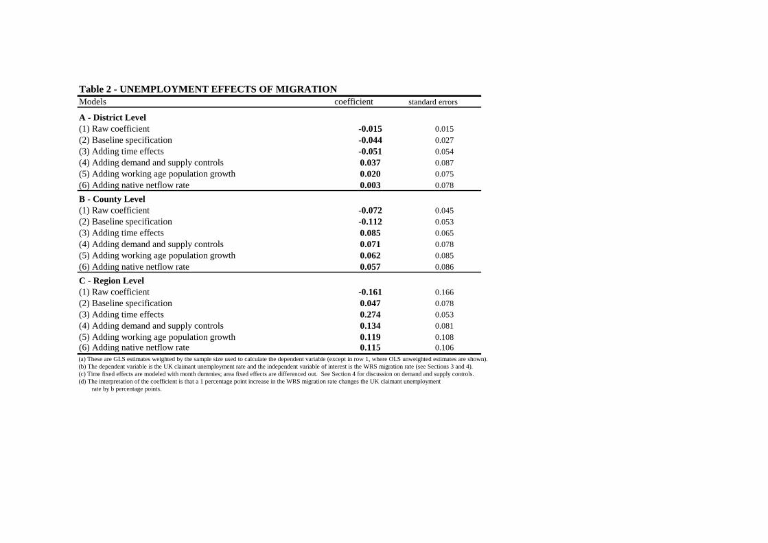
Table 2 - UNEMPLOYMENT EFFECTS OF MIGRATIONModels coefficient standard errors

A - District Level(1) Raw coefficient -0.015 0.015(2) Baseline specification -0.044 0.027(3) Adding time effects -0.051 0.054(4) Adding demand and supply controls 0.037 0.087(5) Adding working age population growth 0.020 0.075(6) Adding native netflow rate 0.003 0.078

B - County Level(1) Raw coefficient -0.072 0.045(2) Baseline specification -0.112 0.053(3) Adding time effects 0.085 0.065(4) Adding demand and supply controls 0.071 0.078(5) Adding working age population growth 0.062 0.085(6) Adding native netflow rate 0.057 0.086

C - Region Level(1) Raw coefficient -0.161 0.166(2) Baseline specification 0.047 0.078(3) Adding time effects 0.274 0.053(4) Adding demand and supply controls 0.134 0.081(5) Adding working age population growth 0.119 0.108(6) Adding native netflow rate 0.115 0.106(a) These are GLS estimates weighted by the sample size used to calculate the dependent variable (except in row 1, where OLS unweighted estimates are shown).(b) The dependent variable is the UK claimant unemployment rate and the independent variable of interest is the WRS migration rate (see Sections 3 and 4). (c) Time fixed effects are modeled with month dummies; area fixed effects are differenced out. See Section 4 for discussion on demand and supply controls.(d) The interpretation of the coefficient is that a 1 percentage point increase in the WRS migration rate changes the UK claimant unemployment rate by b percentage points.

Table 3 - UNEMPLOYMENT EFFECTS OF MIGRANTION (Instrumented)Hansen-Sargan test Hausman test F test

Models coefficient standard errors statistic df statistic df statistic df

A - District Level(1) Lagged migration rates -0.029 0.020 21.95 4 0.02 1 337.75 5 7310(2) Lagged entry-migration rates -0.024 0.023 11.18 3 0.00 1 124.05 4 7718(3) Historic migration rates (Census) -0.144 0.071 0.03 1 3.47 1 109.84 2 8534(4) Historic migration rates (IPS) -0.102 0.140 2.74 1 0.28 1 20.65 2 8534(5) Flight indicator interacted with distance between UK districts and A8 countries -0.137 0.061 23.56 13 2.55 1 17.01 14 8522

B - County Level(1) Lagged migration rates -0.104 0.054 11.36 4 0.00 1 122.77 5 1028(2) Lagged entry-migration rates -0.104 0.062 5.40 3 0.26 1 47.98 4 1087(3) Historic migration rates (Census) -0.106 0.202 3.70 1 0.06 1 15.25 2 1205(4) Historic migration rates (IPS) -0.087 0.244 1.45 1 0.01 1 12.30 2 1205(5) Flight indicator interacted with distance between UK districts and A8 countries -0.139 0.067 22.23 13 1.27 1 16.64 14 1193

C - Region Level(1) Lagged migration rates -0.222 0.134 5.05 4 2.52 1 78.81 5 182(2) Lagged entry-migration rates -0.174 0.169 3.27 3 0.16 1 28.78 4 194(3) Historic migration rates (Census) -0.087 0.174 3.59 1 0.77 1 42.54 2 218(4) Historic migration rates (IPS) -0.045 0.220 0.49 1 0.11 1 22.07 2 218(5) Flight indicator interacted with distance between UK districts and A8 countries -0.072 0.107 9.55 10 2.88 1 24.50 11 211(a) Notes as in Table 2, excetp that these are now GMM estimates.(b) All estimates here to be compared with estimates in row (4) of each respective panel of Table 2.

Table 4 - NATIVE MOBILITY EFFECTS OF MIGRATIONModels coefficient standard errors

A - District Level(1) Raw coefficient -0.182 0.012(2) Baseline specificaiton -0.282 0.005(3) Adding time effects -0.301 0.006(4) Adding working age population growth, wage growth and unemployment rate change -0.293 0.006(5) Adding house prices inflation and vacancies change -0.294 0.006(6) Adding area specific growth rate -0.036 0.001 (6a) Excluding London -0.029 0.002

B - County Level(1) Raw coefficient 0.058 0.022(2) Baseline specificaiton -0.080 0.001(3) Adding time effects -0.098 0.001(4) Adding working age population growth, wage growth and unemployment rate change -0.056 0.002(5) Adding house prices inflation and vacancies change -0.088 0.003(6) Adding area specific growth rate -0.058 0.003 (6a) Excluding London -0.045 0.001

C - Region Level(1) Raw coefficient -0.210 0.109(2) Baseline specificaiton -0.323 0.011(3) Adding time effects -0.539 0.019(4) Adding working age population growth, wage growth and unemployment rate change -0.010 0.004(5) Adding house prices inflation and vacancies change -0.066 0.009(6) Adding area specific growth rate -0.124 0.013 (6a) Excluding London -0.075 0.010(a) Notes as in Table 2, except that the dependent variable is now the native netflow rate (see Section 5.3).

Table 5 - UNEMPLOYMENT EFFECTS OF MIGRATION (robustness checks)Models coefficient standard errors

A - District Level(1) Low Skilled -0.021 0.028(2) Young -0.030 0.033(3) Female 0.015 0.017(4) London Southeast and Eastern 0.051 0.057(5) Agriculture 0.073 0.014

B - County Level(1) Low Skilled 0.043 0.029(2) Young 0.006 0.028(3) Female 0.020 0.013(4) London Southeast and Eastern -0.055 0.014(5) Agriculture 0.043 0.037

C - Region Level(1) Low Skilled 0.043 0.041(2) Young 0.106 0.038(3) Female 0.015 0.024(4) London Southeast and Eastern -0.166 0.278(5) Agriculture -0.014 0.070(a) Notes as in Table 2.(b) All estimates here to be compared with estimates in row (4) of each respective panel of Table 2.

Table 6 - UNEMPLOYMENT EFFECTS OF MIGRATION (by occupation)Models coefficient standard errors

A - Occupation Level(1) Raw coefficient 0.055 0.068(2) Baseline specification 0.019 0.031(3) Adding time effects 0.030 0.038(4) Adding demand and supply controls 0.017 0.025 (4a) Excluding machine operative occupations -0.049 0.089

B - Occupation-Region Level(1) Raw coefficient 0.054 0.022(2) Baseline specification 0.020 0.018(3) Adding time time-area and time-occupation fixed effects 0.030 0.096(4) Adding demand and supply controls 0.056 0.066(a) Notes as in Table 2. As before, time fixed effects are modeled with month dummies. Area and/or occupation fixed effects (and their interaction) are differenced out.

Table 7 - WAGE EFFECTS OF MIGRATIONModels (A) Raw coefficient (B) Baseline specification (C) Adding time effects (D) Adding demand and supply contro

coefficient standard errors coefficient standard errors coefficient standard errors coefficient standard errors

(1) Average wage 0.125 0.230 0.216 0.237 0.252 0.278 0.246 0.276(2) 5th percentile 0.265 0.195 0.380 0.286 0.145 0.187 0.212 0.190(3) 10th percentile -0.249 0.183 -0.383 0.234 0.086 0.226 0.110 0.220(4) 20th percentile -0.553 0.213 -0.428 0.281 0.168 0.299 0.162 0.305(5) 25th percentile -0.260 0.214 -0.135 0.270 0.315 0.305 0.323 0.313(6) 30th percentile -0.209 0.221 -0.030 0.214 0.346 0.234 0.365 0.239(7) 40th percentile -0.129 0.220 0.135 0.216 0.462 0.249 0.453 0.250(8) 50th percentile -0.261 0.241 0.007 0.260 0.469 0.308 0.438 0.307(a) Notes as in Table 2, except that the dependent variable is now the average and various percentiles of the wage distribution across years and districts.