New Developments in Mplus Version 7: Part 3 · New Developments in Mplus Version 7: Part 3 Bengt...
60
New Developments in Mplus Version 7: Part 3 Bengt Muth´ en & Tihomir Asparouhov Mplus www.statmodel.com Presentation at Utrecht University August 2012 Bengt Muth´ en & Tihomir Asparouhov New Developments in Mplus Version 7 1/ 60
Transcript of New Developments in Mplus Version 7: Part 3 · New Developments in Mplus Version 7: Part 3 Bengt...

New Developments in Mplus Version 7:Part 3
Bengt Muthen & Tihomir Asparouhov
Mpluswww.statmodel.com
Presentation at Utrecht UniversityAugust 2012
Bengt Muthen & Tihomir Asparouhov New Developments in Mplus Version 7 1/ 60

Table of Contents I
1 Cross-Classified Analysis, Continued2-Mode Path Analysis: Random Contexts in Gonzalez et al.2-Mode Path Analysis: Monte Carlo SimulationCross-Classified SEMMonte Carlo Simulation of Cross-Classified SEMCross-Classified Models: Types Of Random EffectsRandom Items, Generalizability TheoryRandom Item 2-Parameter IRT: TIMMS ExampleRandom Item Rasch IRT Example
2 Advances in Longitudinal AnalysisBSEM for Aggressive-Disruptive Behavior in the ClassroomCross-Classified Analysis of Longitudinal DataCross-Classified Monte Carlo SimulationCross-Classified Growth Modeling: UG Example 9.27Cross-Classified Analysis of Aggressive-Disruptive Behavior inthe Classroom
Bengt Muthen & Tihomir Asparouhov New Developments in Mplus Version 7 2/ 60

Table of Contents IICross-Classified / Multiple Membership Applications
Bengt Muthen & Tihomir Asparouhov New Developments in Mplus Version 7 3/ 60
Cross-Classified Analysis, Continued
Advanced topics:
2-mode path analysis
Cross-classified SEM
Random item IRT
Bengt Muthen & Tihomir Asparouhov New Developments in Mplus Version 7 4/ 60
2-Mode Path Analysis: Random Contexts in Gonzalez et al.
Gonzalez, de Boeck, Tuerlinckx (2008). A double-structure structuralequation model for three-mode data. Psychological Methods, 13,337-353.
A population of situations that might elicit negative emotionalresponses
11 situations (e.g. blamed for someone else’s failure after asports match, a fellow student fails to return your notes the daybefore an exam, you hear that a friend is spreading gossip aboutyou) viewed as randomly drawn from a population of situations
4 binary responses: Frustration, antagonistic action, irritation,anger
n=679 high school students
Level 2 cluster variables are situations and students
1 observation for each pair of clustering units
Bengt Muthen & Tihomir Asparouhov New Developments in Mplus Version 7 5/ 60

2-Mode Path Analysis: Random Contexts in Gonzalez et al.
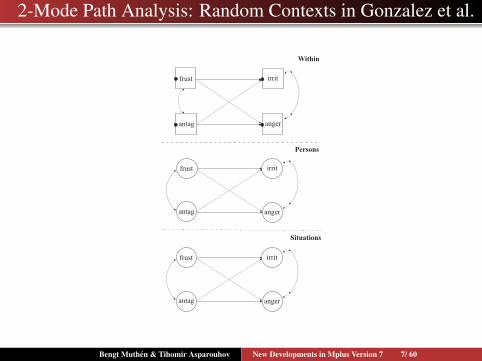
Research questions: Which of the relationships below are significant?Are the relationships the same on the situation level as on the subjectlevel?
Bengt Muthen & Tihomir Asparouhov New Developments in Mplus Version 7 6/ 60
2-Mode Path Analysis: Random Contexts in Gonzalez et al.
���������
�����
� ���
�����
���� ���
�����
����
�����
���
�����
����
�����
���
�����
Bengt Muthen & Tihomir Asparouhov New Developments in Mplus Version 7 7/ 60

2-Mode Path Analysis Input
VARIABLE: NAMES = frust antag irrit anger student situation;CLUSTER = situation student;CATEGORICAL = frust antag irrit anger;
DATA: FILE = gonzalez.dat;ANALYSIS: TYPE = CROSSCLASSIFIED;
ESTIMATOR = BAYES;BITERATIONS = (10000);
MODEL: %WITHIN%irrit anger ON frust antag;irrit WITH anger;frust WITH antag;%BETWEEN student%irrit ON frust (1);anger ON frust (2);irrit ON antag (3);anger ON antag (4);irrit; anger; irrit WITH anger;frust; antag; frust WITH antag;
Bengt Muthen & Tihomir Asparouhov New Developments in Mplus Version 7 8/ 60
2-Mode Path Analysis Input, Continued
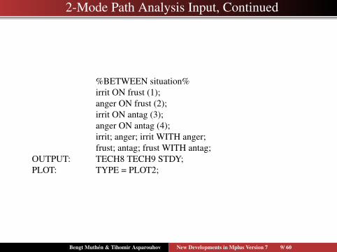
%BETWEEN situation%irrit ON frust (1);anger ON frust (2);irrit ON antag (3);anger ON antag (4);irrit; anger; irrit WITH anger;frust; antag; frust WITH antag;
OUTPUT: TECH8 TECH9 STDY;PLOT: TYPE = PLOT2;
Bengt Muthen & Tihomir Asparouhov New Developments in Mplus Version 7 9/ 60

2-Mode Path Analysis: Monte Carlo Simulation Using theGonzalez Model
M is the number of cluster units for both between levels, β is thecommon slope, ψ is the within-level correlation, τ is the binaryoutcome threshold. Table gives bias (coverage).
Para M=10 M=20 M=30 M=50 M=100β1 0.13(0.92) 0.05(0.89) 0.00(0.97) 0.01(0.92) 0.01(0.94)
ψ2,11 0.11(1.00) 0.06(0.96) 0.01(0.98) 0.00(0.89) 0.02(0.95)ψ2,12 0.15(0.97) 0.06(0.92) 0.05(0.97) 0.03(0.87) 0.01(0.96)
τ1 0.12(0.93) 0.01(0.93) 0.00(0.90) 0.03(0.86) 0.00(0.91)
Small biases for M = 10. Due to parameter equalities information iscombined from both clustering levels. Adding unconstrained level 1model: tetrachoric correlation matrix.
Bengt Muthen & Tihomir Asparouhov New Developments in Mplus Version 7 10/ 60

Cross-Classified SEM
General SEM model: 2-way ANOVA. Ypijk is the p−th variablefor individual i in cluster j and cross cluster k
Ypijk = Y1pijk +Y2pj +Y3pk
3 sets of structural equations - one on each level
Y1ijk = ν +Λ1ηijk + εijk
ηijk = α +B1ηijk +Γ1xijk +ξijk
Y2j = Λ2ηj + εj
ηj = B2ηj +Γ2xj +ξj
Y3k = Λ3ηk + εk
ηk = B3ηk +Γ3xk +ξk
Bengt Muthen & Tihomir Asparouhov New Developments in Mplus Version 7 11/ 60

Cross - Classified SEM
The regression coefficients on level 1 can be a random effectsfrom each of the two clustering levels: combines cross-classifiedSEM and cross classified HLM
Bayesian MCMC estimation: used as a frequentist estimator.
Easily extends to categorical variables.
ML estimation possible only when one of the two level ofclustering has small number of units.
Bengt Muthen & Tihomir Asparouhov New Developments in Mplus Version 7 12/ 60
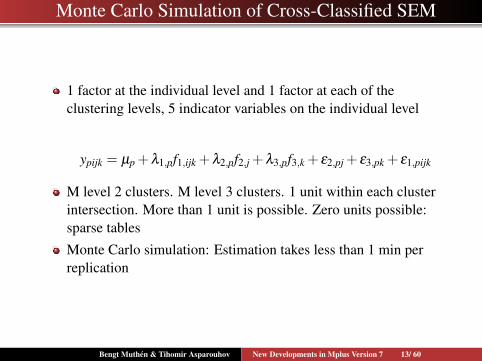
Monte Carlo Simulation of Cross-Classified SEM
1 factor at the individual level and 1 factor at each of theclustering levels, 5 indicator variables on the individual level
ypijk = µp +λ1,pf1,ijk +λ2,pf2,j +λ3,pf3,k + ε2,pj + ε3,pk + ε1,pijk
M level 2 clusters. M level 3 clusters. 1 unit within each clusterintersection. More than 1 unit is possible. Zero units possible:sparse tables
Monte Carlo simulation: Estimation takes less than 1 min perreplication
Bengt Muthen & Tihomir Asparouhov New Developments in Mplus Version 7 13/ 60

Cross-classified model example 1: Factor model results
Table: Absolute bias and coverage for cross-classified factor analysis model
Param M=10 M=20 M=30 M=50 M=100λ1,1 0.07(0.92) 0.03(0.89) 0.01(0.95) 0.00(0.97) 0.00(0.91)θ1,1 0.05(0.96) 0.00(0.97) 0.00(0.95) 0.00(0.99) 0.00(0.94)λ2,p 0.21(0.97) 0.11(0.94) 0.10(0.93) 0.06(0.94) 0.00(0.92)θ2,p 0.24(0.99) 0.10(0.95) 0.04(0.92) 0.05(0.94) 0.02(0.96)λ3,p 0.45(0.99) 0.10(0.97) 0.03(0.99) 0.01(0.92) 0.03(0.97)θ3,p 0.75(1.00) 0.25(0.98) 0.15(0.97) 0.12(0.98) 0.05(0.92)µp 0.01(0.99) 0.04(0.98) 0.01(0.97) 0.05(0.99) 0.00(0.97)
Perfect coverage. Level 1 parameters estimated very well. Biaseswhen the number of clusters is small M = 10. Weakly informativepriors can reduce the bias for small number of clusters.
Bengt Muthen & Tihomir Asparouhov New Developments in Mplus Version 7 14/ 60

Cross-Classified Models: Types Of Random Effects
Type 1: Random slope.%WITHIN%s | y ON x;s has variance on both crossed levels. Dependent variable can bewithin-level factor. Covariate x should be on the WITHIN = list.Type 2: Random loading.%WITHIN%s | f BY y;s has variance on both crossed levels. f is a within-level factor.The dependent variable can be a within-level factor.Type 3: Crossed random loading.%BETWEEN level2a%s | f BY y;s has variance on crossed level 2b and is defined on crossed level2a. f is a level 2a factor, s is a level 2b factor. This is a way touse the interaction term s · f .
Bengt Muthen & Tihomir Asparouhov New Developments in Mplus Version 7 15/ 60
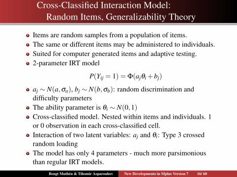
Cross-Classified Interaction Model:Random Items, Generalizability Theory
Items are random samples from a population of items.The same or different items may be administered to individuals.Suited for computer generated items and adaptive testing.2-parameter IRT model
P(Yij = 1) = Φ(ajθi +bj)
aj ∼ N(a,σa), bj ∼ N(b,σb): random discrimination anddifficulty parametersThe ability parameter is θi ∼ N(0,1)Cross-classified model. Nested within items and individuals. 1or 0 observation in each cross-classified cell.Interaction of two latent variables: aj and θi: Type 3 crossedrandom loadingThe model has only 4 parameters - much more parsimoniousthan regular IRT models.
Bengt Muthen & Tihomir Asparouhov New Developments in Mplus Version 7 16/ 60
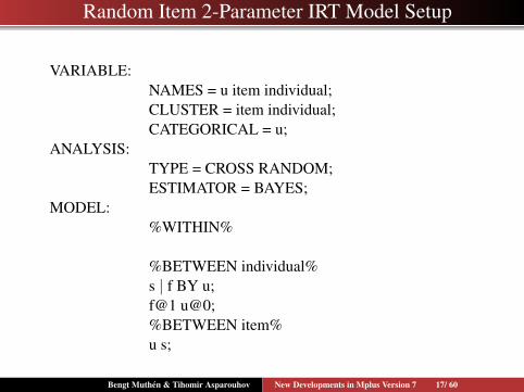
Random Item 2-Parameter IRT Model Setup
VARIABLE:NAMES = u item individual;CLUSTER = item individual;CATEGORICAL = u;
ANALYSIS:TYPE = CROSS RANDOM;ESTIMATOR = BAYES;
MODEL:%WITHIN%
%BETWEEN individual%s | f BY u;f@1 u@0;%BETWEEN item%u s;
Bengt Muthen & Tihomir Asparouhov New Developments in Mplus Version 7 17/ 60

Random Item 2-Parameter IRT: TIMMS Example
Fox (2010) Bayesian Item Response Theory. Section 4.3.3.Dutch Six Graders Math Achievement. Trends in InternationalMathematics and Science Study: TIMMS 20078 test items, 478 students
Table: Random 2-parameter IRT
parameter estimate SEaverage discrimination a 0.752 0.094
average difficulty b 0.118 0.376variation of discrimination a 0.050 0.046
variation of difficulty b 1.030 0.760
8 items means that there are only 8 clusters on the %betweenitem% level and therefore the variance estimates at that level areaffected by their priors. If the number of clusters is less than 10or 20 there is prior dependence in the variance parameters.
Bengt Muthen & Tihomir Asparouhov New Developments in Mplus Version 7 18/ 60
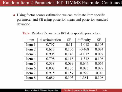
Random Item 2-Parameter IRT: TIMMS Example, Continued
Using factor scores estimation we can estimate item specificparameter and SE using posterior mean and posterior standarddeviation.
Table: Random 2-parameter IRT item specific parameters
item discrimination SE difficulty SEItem 1 0.797 0.11 -1.018 0.103Item 2 0.613 0.106 -0.468 0.074Item 3 0.905 0.148 -1.012 0.097Item 4 0.798 0.118 -1.312 0.106Item 5 0.538 0.099 0.644 0.064Item 6 0.808 0.135 0.023 0.077Item 7 0.915 0.157 0.929 0.09Item 8 0.689 0.105 1.381 0.108
Bengt Muthen & Tihomir Asparouhov New Developments in Mplus Version 7 19/ 60

Random Item 2-Parameter IRT: TIMMS Example,Comparison With ML
Table: Random 2-parameter IRT item specific parameters
Bayes random Bayes random ML fixed ML fixeditem discrimination SE discrimination SE
Item 1 0.797 0.110 0.850 0.155Item 2 0.613 0.106 0.579 0.102Item 3 0.905 0.148 0.959 0.170Item 4 0.798 0.118 0.858 0.172Item 5 0.538 0.099 0.487 0.096Item 6 0.808 0.135 0.749 0.119Item 7 0.915 0.157 0.929 0.159Item 8 0.689 0.105 0.662 0.134
Bayes random estimates are shrunk towards the mean and havesmaller standard errors: shrinkage estimate
Bengt Muthen & Tihomir Asparouhov New Developments in Mplus Version 7 20/ 60

Random Item 2-Parameter IRT: TIMMS Example, Continued
One can add a predictor for a person’s ability. For exampleadding gender as a predictor yields an estimate of 0.283 (0.120),saying that males have a significantly higher math mean.
Predictors for discrimination and difficulty random effects, forexample, geometry indicator.
More parsimonious model can yield more accurate abilityestimates.
Bengt Muthen & Tihomir Asparouhov New Developments in Mplus Version 7 21/ 60
Random Item Rasch IRT Example
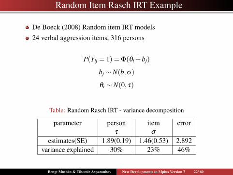
De Boeck (2008) Random item IRT models
24 verbal aggression items, 316 persons
P(Yij = 1) = Φ(θi +bj)
bj ∼ N(b,σ)
θi ∼ N(0,τ)
Table: Random Rasch IRT - variance decomposition
parameter person item errorτ σ
estimates(SE) 1.89(0.19) 1.46(0.53) 2.892variance explained 30% 23% 46%
Bengt Muthen & Tihomir Asparouhov New Developments in Mplus Version 7 22/ 60
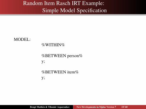
Random Item Rasch IRT Example:Simple Model Specification
MODEL:%WITHIN%
%BETWEEN person%y;
%BETWEEN item%y;
Bengt Muthen & Tihomir Asparouhov New Developments in Mplus Version 7 23/ 60

Advances in Longitudinal Analysis
An old dilemma
Two new solutions
Bengt Muthen & Tihomir Asparouhov New Developments in Mplus Version 7 24/ 60

Categorical Items, Wide Format, Single-Level Approach
Single-level analysis with p×T = 2×5 = 10 variables, T = 5 factors.ML hard and impossible as T increases (numerical integration)WLSMV possible but hard when p×T increases and biasedunless attrition is MCAR or multiple imputation is done firstBayes possibleSearching for partial measurement invariance is cumbersome
Bengt Muthen & Tihomir Asparouhov New Developments in Mplus Version 7 25/ 60

Categorical Items, Long Format, Two-Level Approach
Two-level analysis with p = 2 variables, 1 within-factor, 2-betweenfactors, assuming full measurement invariance across time.
ML feasibleWLSMV feasible (2-level WLSMV)Bayes feasible
Bengt Muthen & Tihomir Asparouhov New Developments in Mplus Version 7 26/ 60

Measurement Invariance Across Time
Both old approaches have problemsWide, single-level approach easily gets significant non-invarianceand needs many modificationsLong, two-level approach has to assume invariance
New solution no. 1, suitable for small to medium number of timepoints
A new wide, single-level approach where time is a fixed modeNew solution no. 2, suitable for medium to large number of timepoints
A new long, two-level approach where time is a random modeNo limit on the number of time points
Bengt Muthen & Tihomir Asparouhov New Developments in Mplus Version 7 27/ 60

New Solution No. 1: Wide Format, Single-Level Approach
Single-level analysis with p×T = 2×5 = 10 variables, T = 5 factors.
Bayes (”BSEM”) using approximate measurement invariance,still identifying factor mean and variance differences across time
Bengt Muthen & Tihomir Asparouhov New Developments in Mplus Version 7 28/ 60
Measurement Invariance Across Time
New solution no. 2, time is a random modeA new long, two-level approach
Best of both worlds: Keeping the limited number of variables ofthe two-level approach without having to assume invariance
Bengt Muthen & Tihomir Asparouhov New Developments in Mplus Version 7 29/ 60

New Solution No. 2: Long Format, Two-Level Approach
Two-level analysis with p = 2 variables.
Bayes twolevel random approach with random measurementparameters and random factor means and variances usingType=Crossclassified: Clusters are time and person
Bengt Muthen & Tihomir Asparouhov New Developments in Mplus Version 7 30/ 60

Aggressive-Disruptive Behavior in the Classroom
Randomized field experiment in Baltimore public schools with aclassroom-based intervention aimed at reducing aggressive-disruptivebehavior among elementary school students (Ialongo et al., 1999).
This analysis:
Cohort 1
9 binary items at 8 time points, Grade 1 - Grade 7
n = 1174
Bengt Muthen & Tihomir Asparouhov New Developments in Mplus Version 7 31/ 60

Aggressive-Disruptive Behavior in the Classroom:ML vs BSEM
Traditional ML analysis8 dimensions of integrationComputing time: 25:44 with Integration = Montecarlo(5000)Increasing the number of time points makes ML impossible
BSEM analysis156 parametersComputing time: 4:01Increasing the number of time points has relatively less impact
Bengt Muthen & Tihomir Asparouhov New Developments in Mplus Version 7 32/ 60

BSEM Input Excerpts for Aggressive-Disruptive Behavior
USEVARIABLES = stub1f-tease7s;CATEGORICAL = stub1f-tease7s;MISSING = ALL (999);
DEFINE: CUT stub1f-tease7s (1.5);ANALYSIS: ESTIMATOR = BAYES;
PROCESSORS = 2;MODEL: f1f by stub1f-tease1f* (lam11-lam19);
f1s by stub1s-tease1s* (lam21-lam29);f2s by stub2s-tease2s* (lam31-lam39);f3s by stub3s-tease3s* (lam41-lam49);f4s by stub4s-tease4s* (lam51-lam59);f5s by stub5s-tease5s* (lam61-lam69);f6s by stub6s-tease6s* (lam71-lam79);f7s by stub7s-tease7s* (lam81-lam89);f1f@1;
Bengt Muthen & Tihomir Asparouhov New Developments in Mplus Version 7 33/ 60
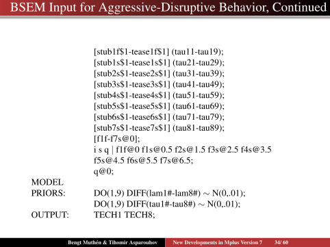
BSEM Input for Aggressive-Disruptive Behavior, Continued
[stub1f$1-tease1f$1] (tau11-tau19);[stub1s$1-tease1s$1] (tau21-tau29);[stub2s$1-tease2s$1] (tau31-tau39);[stub3s$1-tease3s$1] (tau41-tau49);[stub4s$1-tease4s$1] (tau51-tau59);[stub5s$1-tease5s$1] (tau61-tau69);[stub6s$1-tease6s$1] (tau71-tau79);[stub7s$1-tease7s$1] (tau81-tau89);[f1f-f7s@0];i s q | f1f@0 [email protected] [email protected] [email protected] [email protected]@4.5 [email protected] [email protected];q@0;
MODELPRIORS: DO(1,9) DIFF(lam1#-lam8#) ∼ N(0,.01);
DO(1,9) DIFF(tau1#-tau8#) ∼ N(0,.01);OUTPUT: TECH1 TECH8;
Bengt Muthen & Tihomir Asparouhov New Developments in Mplus Version 7 34/ 60
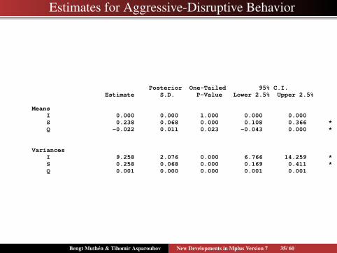
Estimates for Aggressive-Disruptive Behavior
Posterior One-Tailed 95% C.I. Estimate S.D. P-Value Lower 2.5% Upper 2.5% Means I 0.000 0.000 1.000 0.000 0.000 S 0.238 0.068 0.000 0.108 0.366 * Q -0.022 0.011 0.023 -0.043 0.000 * Variances I 9.258 2.076 0.000 6.766 14.259 * S 0.258 0.068 0.000 0.169 0.411 * Q 0.001 0.000 0.000 0.001 0.001
Bengt Muthen & Tihomir Asparouhov New Developments in Mplus Version 7 35/ 60
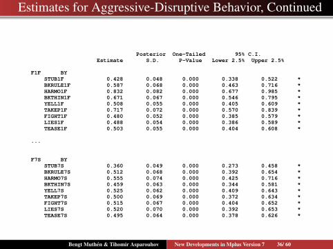
Estimates for Aggressive-Disruptive Behavior, Continued
Posterior One-Tailed 95% C.I. Estimate S.D. P-Value Lower 2.5% Upper 2.5% F1F BY STUB1F 0.428 0.048 0.000 0.338 0.522 * BKRULE1F 0.587 0.068 0.000 0.463 0.716 * HARMO1F 0.832 0.082 0.000 0.677 0.985 * BKTHIN1F 0.671 0.067 0.000 0.546 0.795 * YELL1F 0.508 0.055 0.000 0.405 0.609 * TAKEP1F 0.717 0.072 0.000 0.570 0.839 * FIGHT1F 0.480 0.052 0.000 0.385 0.579 * LIES1F 0.488 0.054 0.000 0.386 0.589 * TEASE1F 0.503 0.055 0.000 0.404 0.608 * ... F7S BY STUB7S 0.360 0.049 0.000 0.273 0.458 * BKRULE7S 0.512 0.068 0.000 0.392 0.654 * HARMO7S 0.555 0.074 0.000 0.425 0.716 * BKTHIN7S 0.459 0.063 0.000 0.344 0.581 * YELL7S 0.525 0.062 0.000 0.409 0.643 * TAKEP7S 0.500 0.069 0.000 0.372 0.634 * FIGHT7S 0.515 0.067 0.000 0.404 0.652 * LIES7S 0.520 0.070 0.000 0.392 0.653 * TEASE7S 0.495 0.064 0.000 0.378 0.626 *
Bengt Muthen & Tihomir Asparouhov New Developments in Mplus Version 7 36/ 60
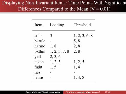
Displaying Non-Invariant Items: Time Points With SignificantDifferences Compared to the Mean (V = 0.01)
Item Loading Threshold
stub 3 1, 2, 3, 6, 8bkrule - 5, 8harmo 1, 8 2, 8bkthin 1, 2, 3, 7, 8 2, 8yell 2, 3, 6 -takep 1, 2, 5 1, 2, 5fight 1, 5 1, 4lies - -tease - 1, 4, 8
Bengt Muthen & Tihomir Asparouhov New Developments in Mplus Version 7 37/ 60

Cross-Classified Analysis of Longitudinal Data
Observations nested within time and subject
A large number of time points can be handled via Bayesiananalysis
A relatively small number of subjects is needed
Bengt Muthen & Tihomir Asparouhov New Developments in Mplus Version 7 38/ 60

Intensive Longitudinal Data
Time intensive data: More longitudinal data are collected wherevery frequent observations are made using new tools for datacollection. Walls & Schafer (2006)Typically multivariate models are developed but if the number oftime points is large these models will fail due to too manyvariables and parameters involvedFactor analysis models will be unstable over time. Is it lack ofmeasurement invariance or insufficient model?Random loading and intercept models can take care ofmeasurement and intercept invariance. A problem becomes anadvantage.Random loading and intercept models produce more accurateestimates for the loadings and factors by borrowing informationover timeRandom loading and intercept models produce moreparsimonious model
Bengt Muthen & Tihomir Asparouhov New Developments in Mplus Version 7 39/ 60

Cross-Classified Analysis: Monte Carlo SimulationGenerating the Data for Ex9.27
TITLE: this is an example of longitudinal modeling using across-classified data approach where observations arenested within the cross-classification of time and subjects
MONTECARLO:NAMES = y1-y3;NOBSERVATIONS = 7500;NREPS = 1;CSIZES = 75[100(1)];! 75 subjects, 100 time pointsNCSIZE = 1[1];WITHIN = (level2a) y1-y3;SAVE = ex9.27.dat;
ANALYSIS:TYPE = CROSS RANDOM;ESTIMATOR = BAYES;PROCESSORS = 2;
Bengt Muthen & Tihomir Asparouhov New Developments in Mplus Version 7 40/ 60

Cross-Classified Analysis: Monte Carlo Simulation, Cont’d
MODELPOPULATION:
%WITHIN%s1-s3 | f by y1-y3;f@1;y1-y3*1.2; [y1-y3@0];%BETWEEN level2a% ! across time variations1-s3*0.1;[s1-s3*1.3];y1-y3*.5;[y1-y3@0];%BETWEEN level2b% ! across subjects variationf*1; [f*.5];s1-s3@0; [s1-s3@0];
Bengt Muthen & Tihomir Asparouhov New Developments in Mplus Version 7 41/ 60
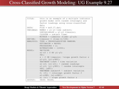
Cross-Classified Growth Modeling: UG Example 9.27
TITLE: this is an example of a multiple indicator
growth model with random intercepts and factor loadings using cross-classified data
DATA: FILE = ex9.27.dat; VARIABLE: NAMES = y1-y3 time subject; USEVARIABLES = y1-y3 timescor; CLUSTER = subject time; WITHIN = timescor (time) y1-y3; DEFINE: timescor = (time-1)/100; ANALYSIS: TYPE = CROSSCLASSIFIED RANDOM; ESTIMATOR = BAYES; PROCESSORS = 2; BITERATIONS = (1000); MODEL: %WITHIN% s1-s3 | f BY y1-y3; f@1; s | f ON timescor; !slope growth factor s y1-y3; [y1-y3@0]; %BETWEEN time% ! time variation s1-s3; [s1-s3]; ! random loadings y1-y3; [y1-y3@0]; ! random intercepts s@0; [s@0]; %BETWEEN subject% ! subject variation f; [f]; ! intercept growth factor f s1-s3@0; [s1-s3@0]; s; [s]; ! slope growth factor s OUTPUT: TECH1 TECH8;
Computing time: 11 minutesBengt Muthen & Tihomir Asparouhov New Developments in Mplus Version 7 42/ 60

Cross-Classified Analysisof Aggressive-Disruptive Behavior in the Classroom
Teacher-rated measurement instrument capturingaggressive-disruptive behavior among a sample of U.S. studentsin Baltimore public schools (Ialongo et al., 1999).The instrument consists of 9 items scored as 0 (almost never)through 6 (almost always)A total of 1174 students are observed in 41 classrooms from Fallof Grade 1 through Grade 6 for a total of 8 time pointsThe multilevel (classroom) nature of the data is ignored in thecurrent analysesThe item distribution is very skewed with a high percentage inthe Almost Never category. The items are thereforedichotomized into Almost Never versus the other categoriescombinedWe analyze the data on the original scale as continuous variablesand also the dichotomized scale as categorical
Bengt Muthen & Tihomir Asparouhov New Developments in Mplus Version 7 43/ 60
Aggressive-Disruptive Behavior Example Continued
For each student a 1-factor analysis model is estimated with the 9items at each time point
Let Ypit be the p−th item for individual i at time t
We use cross-classified SEM. Observations are nested withinindividual and time.
Although this example uses only 8 time points the models can beused with any number of time points.
Bengt Muthen & Tihomir Asparouhov New Developments in Mplus Version 7 44/ 60
Aggressive-Disruptive Behavior Example Cont’d: Model 1
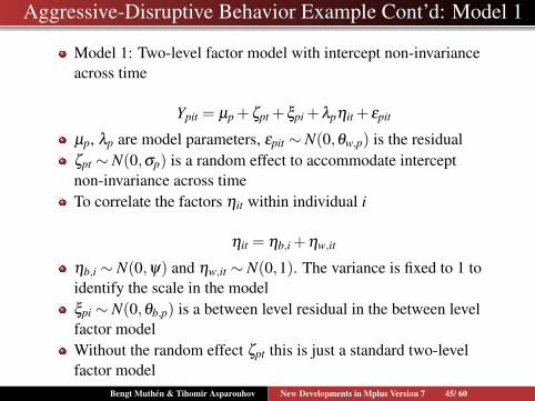
Model 1: Two-level factor model with intercept non-invarianceacross time
Ypit = µp +ζpt +ξpi +λpηit + εpit
µp, λp are model parameters, εpit ∼ N(0,θw,p) is the residualζpt ∼ N(0,σp) is a random effect to accommodate interceptnon-invariance across timeTo correlate the factors ηit within individual i
ηit = ηb,i +ηw,it
ηb,i ∼ N(0,ψ) and ηw,it ∼ N(0,1). The variance is fixed to 1 toidentify the scale in the modelξpi ∼ N(0,θb,p) is a between level residual in the between levelfactor modelWithout the random effect ζpt this is just a standard two-levelfactor model
Bengt Muthen & Tihomir Asparouhov New Developments in Mplus Version 7 45/ 60
Aggressive-Disruptive Behavior Example Continued:Model 1 Setup
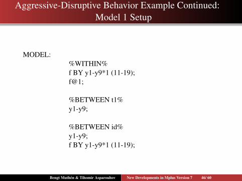
MODEL:%WITHIN%f BY y1-y9*1 (11-19);f@1;
%BETWEEN t1%y1-y9;
%BETWEEN id%y1-y9;f BY y1-y9*1 (11-19);
Bengt Muthen & Tihomir Asparouhov New Developments in Mplus Version 7 46/ 60

Aggressive-Disruptive Behavior Example Cont’d: Model 2
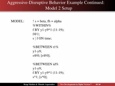
Model 2: Adding latent growth model for the factor
ηit = αi +βi · t +ηw,it
αi ∼ N(0,vα) is the intercept and βi ∼ N(β ,vβ ) is the slope. Foridentification purposes again ηw,it ∼ N(0,1)The model looks for developmental trajectory across time for theaggressive-disruptive behavior factor
Bengt Muthen & Tihomir Asparouhov New Developments in Mplus Version 7 47/ 60
Aggressive-Disruptive Behavior Example Continued:Model 2 Setup
MODEL: ! s = beta, fb = alpha%WITHIN%f BY y1-y9*1 (11-19);f@1;s | f ON time;
%BETWEEN t1%y1-y9;s@0; [s@0];
%BETWEEN id%y1-y9;f BY y1-y9*1 (11-19);s*1; [s*0];
Bengt Muthen & Tihomir Asparouhov New Developments in Mplus Version 7 48/ 60
Aggressive-Disruptive Behavior Example Cont’d: Model 3
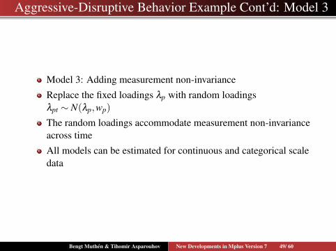
Model 3: Adding measurement non-invariance
Replace the fixed loadings λp with random loadingsλpt ∼ N(λp,wp)The random loadings accommodate measurement non-invarianceacross time
All models can be estimated for continuous and categorical scaledata
Bengt Muthen & Tihomir Asparouhov New Developments in Mplus Version 7 49/ 60
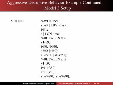
Aggressive-Disruptive Behavior Example Continued:Model 3 Setup
MODEL: %WITHIN%s1-s9 | f BY y1-y9;f@1;s | f ON time;%BETWEEN t1%y1-y9;f@0; [f@0];s@0; [s@0];s1-s9*1; [s1-s9*1];%BETWEEN id%y1-y9;f*1; [f@0];s*1; [s*0];s1-s9@0; [s1-s9@0];
Bengt Muthen & Tihomir Asparouhov New Developments in Mplus Version 7 50/ 60

Aggressive-Disruptive Behavior Example Continued:Model 3 Results For Continuous Analysis
Bengt Muthen & Tihomir Asparouhov New Developments in Mplus Version 7 51/ 60
Aggressive-Disruptive Behavior Example Cont’d: Model 4
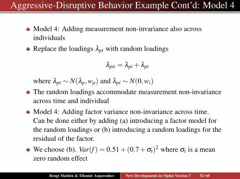
Model 4: Adding measurement non-invariance also acrossindividuals
Replace the loadings λpt with random loadings
λpit = λpi +λpt
where λpt ∼ N(λp,wp) and λpi ∼ N(0,wi)The random loadings accommodate measurement non-invarianceacross time and individual
Model 4: Adding factor variance non-invariance across time.Can be done either by adding (a) introducing a factor model forthe random loadings or (b) introducing a random loadings for theresidual of the factor.
We choose (b). Var(f ) = 0.51+(0.7+σt)2 where σt is a meanzero random effect
Bengt Muthen & Tihomir Asparouhov New Developments in Mplus Version 7 52/ 60
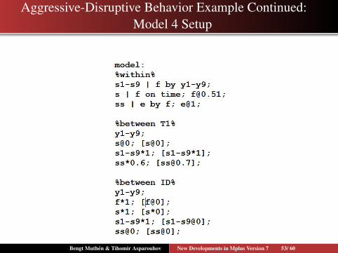
Aggressive-Disruptive Behavior Example Continued:Model 4 Setup
Bengt Muthen & Tihomir Asparouhov New Developments in Mplus Version 7 53/ 60
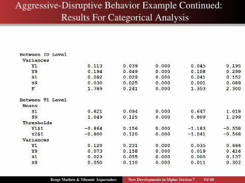
Aggressive-Disruptive Behavior Example Continued:Results For Categorical Analysis
Bengt Muthen & Tihomir Asparouhov New Developments in Mplus Version 7 54/ 60

Aggressive-Disruptive Behavior Example Conclusions
Other extensions of the above model are possible, for examplethe growth trend can have time specific random effects: f and scan be free over timeThe more clusters there are on a particular level the moreelaborate the model can be on that level. However, the moreelaborate the model on a particular level is, the slower theconvergenceThe main factor f can have a random effect on each of the levels,however the residuals Yi should be uncorrelated on that level. Ifthey are correlated through another factor model such as,fb by y1− y9, then f would be confounded with that factor fband the model will be poorly identifiedOn each level the most general model would be (if there are norandom slopes) the unconstrained variance covariance for thedependent variables Yi. Any model that is a restriction of thatmodel is in principle identified
Bengt Muthen & Tihomir Asparouhov New Developments in Mplus Version 7 55/ 60

Aggressive-Disruptive Behavior Example Conclusions,Continued
Unlike ML and WLS multivariate modeling, for the timeintensive Bayes cross-classified SEM, the more time points thereare the more stable and easy to estimate the model is
Bayesian methods solve problems not feasible with ML or WLS
Time intensive data naturally fits in the cross-classified modelingframework
Asparouhov and Muthen (2012). General Random Effect LatentVariable Modeling: Random Subjects, Items, Contexts, andParameters
Bengt Muthen & Tihomir Asparouhov New Developments in Mplus Version 7 56/ 60

Cross-Classified / Multiple Membership Applications
Jeon & Rabe-Hesketh (2012). Profile-Likelihood Approach forEstimating Generalized Linear Mixed Models With FactorStructures. JEBS
Longitudinal growth model for student self-esteem
Each student has 4 observations: 2 in middle school in wave 1and 2, and 2 in high school in wave 3 and 4
Students have multiple membership: Membership in middleschool and in high school with a random effect from both
Ytsmh is observation at time t for student s in middle school m andhigh school h
Bengt Muthen & Tihomir Asparouhov New Developments in Mplus Version 7 57/ 60

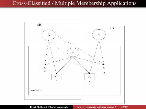
Cross-Classified / Multiple Membership Applications
The model is
Ytsmh = β1 +β2T2+β3T3+β4T4+δs +δmµt +δhλt + εtsmh
where T2, T3, T4 are dummy variables for wave 2, 3, 4
δs, δm and δh are zero mean random effect contributions fromstudent, middle school and high school
µt = (1,µ2,µ3,µ4)λt = (0,0,1,λ4), i.e., no contribution from the high school inwave 1 and 2 because the student is still in middle school
εtsmh is the residual
Very simple to setup in Mplus
Bengt Muthen & Tihomir Asparouhov New Developments in Mplus Version 7 58/ 60
Cross-Classified / Multiple Membership Applications
Bengt Muthen & Tihomir Asparouhov New Developments in Mplus Version 7 59/ 60
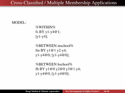
Cross-Classified / Multiple Membership Applications
MODEL:%WITHIN%fs BY y1-y4@1;[y1-y4];
%BETWEEN mschool%fm BY y1@1 y2-y4;y1-y4@0; [y1-y4@0];
%BETWEEN hschool%fh BY y1@0 y2@0 y3@1 y4;y1-y4@0; [y1-y4@0];
Bengt Muthen & Tihomir Asparouhov New Developments in Mplus Version 7 60/ 60