NEW COUNTEREXAMPLES TO THE CELL FORMULA IN NONCONVEX HOMOGENIZATION€¦ · NEW COUNTEREXAMPLES TO...
30
NEW COUNTEREXAMPLES TO THE CELL FORMULA IN NONCONVEX HOMOGENIZATION MARCO BARCHIESI & ANTOINE GLORIA Abstract. In this article we show that for the homogenization of multiple integrals, the quasiconvexification of the cell formula is different from the asymptotic formula in general. To this aim, we construct three examples in three different settings: the homogenization of a discrete model, the homogenization of a composite material and the homogenization of a homogeneous material on a perforated domain. Keywords: homogenization, quasiconvexity, cell formula 2000 Mathematics Subject Classification: 35B27, 49J45, 73B27, 74E30, 74Q05. Contents 1. Introduction 1 2. Homogenization of multiple integrals and the cell formula 3 2.1. Continuous and discrete homogenization of nonconvex functionals 3 2.2. Short summary of convexity properties 5 2.3. Stefan M¨ uller’s counterexample 9 2.4. Counterexample by comparison of the zero levelsets 11 3. Counterexamples from composite materials 11 3.1. Discrete example 12 3.2. An example from solid-solid phase transformations 14 3.3. Comparison of boths examples 18 4. Counterexample on perforated domains 18 Appendix: Stefan M¨ uller’s example in dimension three 25 References 29 1. Introduction For the homogenization of periodic integral functionals of the type I ε (u) := Ω∩εP W ( x ε , ∇u(x) ) dx, with suitable assumptions (recalled in Section 2.1), the Γ-limit writes I hom (u) := Ω W hom ( ∇u(x) ) dx, where W hom is obtained by an asymptotic formula on the number of periodic cells con- sidered. If the integrand W (x, ·) happens to be convex almost everywhere, then the Date : August 29, 2008. 1
Transcript of NEW COUNTEREXAMPLES TO THE CELL FORMULA IN NONCONVEX HOMOGENIZATION€¦ · NEW COUNTEREXAMPLES TO...

NEW COUNTEREXAMPLES TO THE CELL FORMULA IN
NONCONVEX HOMOGENIZATION
MARCO BARCHIESI & ANTOINE GLORIA
Abstract. In this article we show that for the homogenization of multiple integrals,the quasiconvexification of the cell formula is different from the asymptotic formulain general. To this aim, we construct three examples in three different settings: thehomogenization of a discrete model, the homogenization of a composite material andthe homogenization of a homogeneous material on a perforated domain.
Keywords: homogenization, quasiconvexity, cell formula
2000 Mathematics Subject Classification: 35B27, 49J45, 73B27, 74E30, 74Q05.
Contents
1. Introduction 12. Homogenization of multiple integrals and the cell formula 32.1. Continuous and discrete homogenization of nonconvex functionals 32.2. Short summary of convexity properties 52.3. Stefan Muller’s counterexample 92.4. Counterexample by comparison of the zero levelsets 113. Counterexamples from composite materials 113.1. Discrete example 123.2. An example from solid-solid phase transformations 143.3. Comparison of boths examples 184. Counterexample on perforated domains 18Appendix: Stefan Muller’s example in dimension three 25References 29
1. Introduction
For the homogenization of periodic integral functionals of the type
Iε(u) :=
∫
Ω∩εPW(xε,∇u(x)
)dx,
with suitable assumptions (recalled in Section 2.1), the Γ-limit writes
Ihom(u) :=
∫
ΩWhom
(∇u(x)
)dx,
where Whom is obtained by an asymptotic formula on the number of periodic cells con-sidered. If the integrand W (x, ·) happens to be convex almost everywhere, then the
Date: August 29, 2008.
1
2 M. BARCHIESI & A. GLORIA
asymptotic formula reduces to a minimization problem on the unitary cell with periodicboundary conditions, that we denote by Wcell. A counterexample due to Stefan Mullerin [12] shows that in general, for quasiconvex nonconvex energy densities, the inequalityWcell ≥ Whom can be strict. More recently, Jean-Francois Babadjian and the first authorgave another such example in [3].
As will be made precise in Section 2 for both examples, the energy density Wcell is notrank-one convex. In addition, in both cases, considering the quasiconvex envelop QWcell ofWcell surprisingly removes the contradiction which allows to conclude that Wcell > Whom.Hence, none of the known examples shows that the inequality QWcell ≥ Whom can bestrict, although this is to be expected.
The aim of this paper is twofold: to show that the known counterexamples to thecell formula are not rigid enough to prove that QWcell > Whom, and then to providesome new examples for which the latter strict inequality can be shown. The article isorganized as follows. In Section 2, we recall standard results on homogenization as wellas the two counterexamples to the cell formula mentioned above. We then show for eachexample that the methods used by their respective authors to prove the disagreement ofWcell with Whom fail to prove the disagreement of QWcell with Whom. The rest of thepaper is then dedicated to the construction of three different examples for which thereexists a deformation gradient Λ such that QWcell(Λ) > Whom(Λ). The examples are builtin dimension two and they are based on the fact that replacing (0, 1)2-periodicity by(0, 2)2-periodicity is enough to relax significantly the energy to obtain the desired strictinequality. The first example is a discrete example where the keyrole is played by the verystrong rigidity of discrete gradients. The second example is based on the same geometrybut is written in a continuous setting and exploits the rigidity of the incompatible two-well problem together with an interplay between the geometry, the periodicity and thezero levelset of the energy densities. These examples are presented in Section 3. Thelast example is the object of Section 4. It relies on the homogenization of a homogeneousmaterial on a perforated domain, for which we prove that the zero levelset of Wcell iscontained in a quasiconvex set which is strictly contained in the zero levelset of Whom.This is in particular the first example which shows the disagreement of Wcell and Whom
(as well as QWcell and Whom) for the homogenization of a homogeneous material on aperforated domain.
Although the main result of this article is technical, we believe the examples are ofindependent interest. We therefore provide the non-specialist reader with the requiredbackground on convexity properties in Section 2.2.
Throughout the paper, we employ the following notation:
• Ω is a bounded open subset of Rd;
• Q = (0, 1)d denotes the unit cell;• Qn = (0, n)d for all n ∈ N;• Qm = m+Q for all m ∈ Z
d;• χU is the characteristic function of a subset U of R
d;• M
d is the set of d× d real matrices;• M
dsym is the set of d× d symmetric real matrices;
• SOd is the family of the elements Λ of Md such that det Λ = 1 and ΛT Λ = I, where
I ∈ Md is the identity matrix;
COUNTEREXAMPLES IN NONCONVEX HOMOGENIZATION 3
• |Λ| :=√
trace(ΛT Λ) is the Frobenius norm of a matrix Λ ∈ Md;
• Ln denotes the n-dimensional Lebesgue measure;• W 1,p
per(Qn,Rd) is the space of W 1,p
loc (Rd; Rd) functions which are Qn-periodic;• As a general rule, c denotes a constant which may vary from line to line but which
is independent of the variables left.
2. Homogenization of multiple integrals and the cell formula
2.1. Continuous and discrete homogenization of nonconvex functionals. In thissection, we recall classical results of periodic homogenization of multiple integrals, aswell as (less) classical results of periodic homogenization of discrete systems. We referthe reader to the monograph [7] for continuous homogenization and to the article [1] fordiscrete homogenization.
Definition 1. Let U be a normed space. We say that I : U → [−∞,+∞] is the Γ-limitof a sequence Ih : U → [−∞,+∞], or that Ih Γ-converges to I, if for every u ∈ U thefollowing conditions are satisfied:
i) Liminf inequality : for every sequence uh in U such that uh → u,
I(u) ≤ lim infh→+∞
Ih(uh);
ii) Recovery sequence: there exists a sequence uh in U such that uh → u and
I(u) = limh→+∞
Ih(uh).
Let d ∈ N. We focus on Γ-convergence of integral functionals on the normed spaceLp(Ω,Rd), p ∈ (1,+∞), in the context of periodic homogenization.
Let a > 0. We denote by W(a, p) the set of all continuous functions W : Md → [0,+∞)
satisfying the following coerciveness and growth conditions of order p:
1
a|Λ|p − a ≤ W(Λ) ≤ a(1 + |Λ|p) for all Λ ∈ M
d. (2.1)
Hypothesis 1. W : Rd × M
d → [0,+∞) is a Caratheodory function Q-periodic in thefirst variable such that W (x, ·) ∈ W(a, p) for a.e x ∈ Q.
Hypothesis 2. P is a Q-periodic and open subset of Rd with Lipschitz boundary such
that Q \ P ⊂⊂ Q. Note that in particular P is connected.
Under Hypotheses 1 and 2, we consider for any ε > 0 the functional Iε : Lp(Ω,Rd) →[0,+∞] defined by
Iε(u) :=
∫
Ω∩εPW(xε,∇u(x)
)dx if u|Ω∩εP ∈W 1,p(Ω ∩ εP,Rd),
+∞ otherwise.
Definition 2. We call cell integrand related to (W,P ) the function Wcell : Md → [0,+∞)
defined by
Wcell(Λ) := inf∫
Q∩PW(x,Λ + ∇φ(x)
)dx : φ ∈W 1,p
per(Q,Rd). (2.2)

4 M. BARCHIESI & A. GLORIA
If P = Rd we simply say that Wcell is the cell integrand related to W .
We call homogenized integrand related to (W,P ) the function Whom : Md → [0,+∞)
defined by
Whom(Λ) := limn→∞
1
ndinf∫
Qn∩PW(x,Λ + ∇φ(x)
)dx : φ ∈W 1,p
per(Qn,Rd).
If P = Rd we simply say that Whom is the homogenized integrand related to W .
The following theorem is a standard result (See [7, Theorem 19.1 and Remark 19.2]).
Theorem 1. Assume that W satisfies Hypothesis 1 and that P satisfies Hypothesis 2.Then the homogenized integrand Whom related to (W,P ) is a quasiconvex function satis-fying (2.1), and for any εh ց 0+ the sequence Iεh
Γ-converges to the functional Ihom :Lp(Ω,Rd) → [0,+∞] defined by
Ihom(u) :=
∫
ΩWhom
(∇u(x)
)dx if u ∈W 1,p(Ω,Rd),
+∞ otherwise.
In addition, if W (x, ·) is convex for a.e. x ∈ Q, then Whom is also convex and coincideswith the cell integrand Wcell related to (W,P ).
A result similar to Theorem 1 holds in a discrete setting, as shown in [1]. We give herea simpler version, for which we only consider nearest-neighbors interactions. We also needto slightly extend the result in [1] to take into account volumetric effects, which we willneed in Section 3. Yet, the result remains essentially the same and further details can befound in [2].
Definition 3. Let T be a Q-periodic triangulation of Rd and P be the set of vertices of
T . We define the couples of nearest neighbors by
NN :=(x, y) ∈ (P ∩Q)2 : ∃T ∈ T having [x, y] as an edge
.
For all ε > 0 and for all bounded open subset U of Rd, we define
Sε(U,Rd) :=
u ∈ C0(U,Rd) : u is affine on each element T ∈ εT ∩ U
.
For ε = 1, we simply write S(U,Rd) = Sε(U,Rd). Moreover, we write
Sper(Qn,Rd) := S(Qn,R
d) ∩W 1,∞per (Qn,R
d).
We are now in position to define energy functionals on discrete systems.
Definition 4. Let f1 : Q ×Q× Rd → [0,+∞) and f2 : Q× R → [0,+∞) be continuous
functions and let ε > 0. For any bounded open subset U of Rd, we define the energy of
u ∈ Sε(U,Rd) as
Fε(u,U) :=∑
m∈Zd : εQm⊆U
Fmε (u),
where, for any m ∈ Zd such that εQm ⊆ U ,
Fmε (u) := εd
∑
(x,y)∈NN
f1
(x, y,
u(εm+ εx) − u(εm+ εy)
ε|x− y|
)+εd
∫
Qf2
(x,det∇u(εm+εx)
)dx.
COUNTEREXAMPLES IN NONCONVEX HOMOGENIZATION 5
If ε = 1, we simply write F (u,U) = Fε(u,U). Finally, we define the functional Iε :Lp(Ω,Rd) → [0,+∞] by
Iε(u) :=
Fε(u,Ω) if u ∈ Sε(Ω,R
d),
+∞ otherwise.
As for the continuous setting, we may define a cell integrand and a homogenized inte-grand as follows.
Definition 5. For all Λ ∈ Md, let ϕΛ : R
d → Rd be given by ϕΛ(x) := Λ · x. We call cell
integrand related to (T , F ) the function Wcell : Md → [0,+∞) defined by
Wcell(Λ) := infF (ϕΛ + φ,Q) : φ ∈ Sper(Q,R
d).
We call homogenized integrand related to (T , F ) the function Whom : Md → [0,+∞)
defined by
Whom(Λ) := limn→∞
1
ndinfF (ϕΛ + φ,Qn) : φ ∈ Sper(Qn,R
d).
We have the following result (see [1] and [2]).
Theorem 2. Let T , f1, f2, Iε and Whom be as in Definitions 3, 4, 5. Let us furtherassume that there exist a > 0 and p ∈ (1,∞) such that
0 ≤ f2(x, z) ≤ a(1 + |z|p/d) for all (x, z) ∈ Q× R,
1
a|w|p − a ≤ f1(x, y,w) ≤ a(1 + |w|p) for all (x, y,w) ∈ Q×Q× R
d,
Then the homogenized integrand Whom associated to (T , F ) is a quasiconvex function sat-isfying a growth condition (2.1), and for any εh ց 0+ the sequence Iεh
Γ-converges to thefunctional Ihom : Lp(Ω,Rd) → [0,+∞] defined by
Ihom(u) :=
∫
ΩWhom
(∇u(x)
)dx if u ∈W 1,p(Ω,Rd),
+∞ otherwise.
In addition, if f2 ≡ 0 and if f1(x, y, ·) is a convex function for all x, y ∈ Q, then Whom is
also convex and coincides with the cell integrand Wcell related to (T , F ).
2.2. Short summary of convexity properties. In this section, we recall the notionsof polyconvexity, quasiconvexity and rank-one convexity of functions and sets. We referthe reader to [8, 9, 13] for details. We also state and prove some elementary lemmas thatwill be used in the analysis of the counterexamples.
Definition 6. (quasiconvex function) Let W : Md → R be locally bounded and Borel
measurable. Its quasiconvex envelope QW : Md → [−∞,+∞) is defined by
QW (Λ) := inf
−∫
UW(Λ + ∇φ(x)
)dx : φ ∈W 1,∞
0 (U,Rd)
,
where U is a bounded open subset of Rd. In particular, the infimum in the formula
is independent of the choice of U . If U = Q, then W 1,∞0 (Q,Rd) can be replaced by

6 M. BARCHIESI & A. GLORIA
W 1,∞per (Q,Rd). The function W is said to be quasiconvex if W = QW . If QW is finite,
then it is quasiconvex.
Lemma 1. (main property) Let W : Ω× Md → [0,+∞) be a Caratheodory function such
that W (x, ·) ∈ W(a, p) for a.e. x ∈ Ω and let U be a weakly closed subset of W 1,p(Ω,Rd).Then
inf
∫
ΩW(x,∇u(x)
)dx : u ∈ U
= min
∫
ΩQW
(x,∇u(x)
)dx : u ∈ U
> −∞,
and any weak limit of a minimizing sequence of the original problem is a minimizer of therelaxed problem.
Remark 1. Assume that P satisfies Hypothesis 2. Since Q ∩ P has Lipschitz boundary,any function ϕ ∈ W 1,p(Q ∩ P,Rd) can be extended to a function ϕ ∈ W 1,p(Q,Rd). As a
consequence, φ|Q∩P : φ ∈W 1,pper(Q,Rd) is a weakly closed subset of W 1,p(Q ∩ P,Rd).
Definition 7. (polyconvex function) For any matrix Λ ∈ Md, let denote by M(Λ) the
vector that consists of all minors of Λ, and denote by δ(d) its length. We can identifyM(Λ) with a point of R
δ(d). We say that a function W : Md → R is polyconvex if there
exists a convex function g : Rδ(d) → R such that for all Λ ∈ M
d,
W (Λ) = g(M(Λ)).
Definition 8. (rank-one convex function) We say that W : Md → R is rank-one convex if
W (tA+ (1 − t)B) ≤ tW (A) + (1 − t)W (B)
for all t ∈ [0, 1] and for all A,B ∈ Md rank-one connected, i.e., such that rank(B−A) = 1.
Lemma 2. Let W : Md → R, then there holds
W is convex =⇒ W is polyconvex =⇒ W is quasiconvex =⇒ W is rank-one convex.
One can extend the notions of convexity, polyconvexity, quasiconvexity and rank-oneconvexity to sets.
Definition 9. (polyconvex, quasiconvex and rank-one convex sets) Let K be a compactsubset of M
d. We define the polyconvex hull Kpc, quasiconvex hull Kqc and rank-oneconvex hull Krc of K by
Kpc :=Λ ∈ M
d : f(Λ) = 0 ∀ f : Md → [0,+∞) polyconvex such that f |K ≡ 0
,
Kqc :=Λ ∈ M
d : f(Λ) = 0 ∀ f : Md → [0,+∞) quasiconvex such that f |K ≡ 0
,
Krc :=Λ ∈ M
d : f(Λ) = 0 ∀ f : Md → [0,+∞) rank-one convex such that f |K ≡ 0
.
The set K is said to be polyconvex if K = Kpc, quasiconvex if K = Kqc and rank-one convex if K = Krc. We have the inclusions Krc ⊆ Kqc ⊆ Kpc ⊆ Kco, where thesuperscript co denotes the classical convex hull.
We have the following useful characterizations of Kqc and Kpc.
Lemma 3. ([13, Theorem 4.10]). Given a compact set K ⊆ Md, a matrix A ∈ M
d belongsto Kqc if and only if there exists a sequence ψh bounded in W 1,∞(Q,Rd) such that
dist(∇ψh,K) → 0 in measure;
ψh(x) = A · x for x ∈ ∂Q.

COUNTEREXAMPLES IN NONCONVEX HOMOGENIZATION 7
Lemma 4. ([11, Lemma 1]). Given a compact set K ⊆ Md, a matrix A ∈ M
d belongs toKpc if and only if M(A) lies in M(Λ) : Λ ∈ Kco.
The sets we will be interested in are the zero-levelsets of energy densities defined asfollows.
Definition 10. Let W : Md → [0,+∞) be a continuous function, we define its zero
levelset as
W−1(0) =Λ ∈ M
d : W (Λ) = 0.
In particular, if W is a quasiconvex function, then W−1(0) is a quasiconvex set.
Lemma 5. If W ∈ W(a, p), then
QW−1(0) = (W−1(0))qc.
Proof. Let K := W−1(0). The inclusion Kqc ⊆ QW−1(0) is trivial and we only need toprove the opposite one. This proof makes use of Young measures, for which we refer thereader to [13] for a comprehensive treatment.
Let A ∈ QW−1(0). By definition of the quasiconvex envelope, there exists φh ∈W 1,∞
0 (Q,Rd) such that
0 = QW (A) = limh→+∞
∫
QW(A+ ∇φh(x)
)dx.
As a consequence of the p-coercivity of W and Poincare’s inequality, the sequence ψh(x) :=A · x+ φh(x) is bounded in W 1,p(Q,Rd). Thus, up to extraction, ∇ψh generates a Youngmeasure µ : Q ∋ x 7→ µx ∈ P(Md), where P(Md) denotes the family of probabilitymeasures on M
d.By the fundamental theorem on Young measures (see [13, Theorem 3.1]), we get
0 = limh→+∞
∫
QW(A+ ∇φh(x)
)dx ≥
∫
Q
(∫
Md
W (Λ)dµx(Λ))dx
and therefore by [5, Lemma 3.3] suppµx ⊆ K for Lda.e. x ∈ Q. Again by the fundamentaltheorem, this implies that
dist(∇ψh,K) → 0 in measure. (2.3)
By using Zhang’s lemma (see [13, Lemma 4.21]), ψh can be modified on small sets so thatits gradient be bounded in L∞(Q,Md), while keeping conditions (2.3) and ψh(x) = A · xfor x ∈ ∂Q. The thesis follows now by Lemma 3.
We will also make use of the following results about the cell integrand.
Lemma 6. Assume that W satisfies Hypothesis 1 and that P satisfies Hypothesis 2. Thenthe cell integrand Wcell related to (W,P ) is a continuous function.
Proof. This property is a direct consequence of the following inequality:
Wcell(Λ1) ≤Wcell(Λ2) + c(Λ1,Λ2)|Λ1 − Λ2| for all Λ1,Λ2 ∈ Md, (2.4)
where c(Λ1,Λ2) is locally uniformly bounded.

8 M. BARCHIESI & A. GLORIA
Let us prove inequality (2.4). By Lemma 1 and Remark 1, we have
Wcell(Λ) = min
∫
Q∩PQW
(x,Λ + ∇φ(x)
)dx : φ ∈W 1,p
per(Q,Rd)
. (2.5)
Due to the growth condition from above satisfied by QW (x, ·), there exists c > 0 suchthat for every Λ1,Λ2 ∈ M
d, there holds
|QW (x,Λ1) −QW (x,Λ2)| ≤ c|Λ1 − Λ2|(1 + |Λ1|p−1 + |Λ2|p−1)
This property, which is classical for convex functions, holds for rank-one convex functions(see [10, Lemma 5.2]). Let now Λ1,Λ2 ∈ M
d, and let φ1, φ2 ∈ W 1,pper(Q,Rd) be minimizers
associated with Λ1 and Λ2 through (2.5). We then have
Wcell(Λ1) −Wcell(Λ2) =
∫
Q∩PQW
(x,Λ1 + ∇φ1(x)
)−QW
(x,Λ2 + ∇φ2(x)
)dx
≤∫
Q∩PQW
(x,Λ1 + ∇φ2(x)
)−QW
(x,Λ2 + ∇φ2(x)
)dx
≤∫
Q∩Pc|Λ1 − Λ2|(1 + |Λ1|p−1 + |Λ2|p−1 + |Λ2 + ∇φ2(x)|p−1)dx.
Using the coercivity of QW (lower bound in (2.1)), we may bound ‖Λ2 + ∇φ2‖pLp from
above by the energy, which is less than c(1 + |Λ2|p) using the test function φ ≡ 0 and theupper bound of (2.1). Hence, there exists a constant c > 0 such that the inequality
Wcell(Λ1) −Wcell(Λ2) ≤ c|Λ1 − Λ2|(1 + |Λ1|p−1 + |Λ2|p−1),
holds for any Λ1,Λ2 ∈ Md, which proves the claim.
Lemma 7. Let W ∈ W(a, p) and let P satisfy Hypothesis 2. Assume in addition that Wis quasiconvex, and that W−1(0) is not empty. Then A ∈ Md belongs to the zero levelsetof the cell integrand Wcell associated to (W,P ) if and only if there exists a Q-periodicLipschitz function φ : R
d → Rd satisfying
A+ ∇φ(x) ∈W−1(0) for a.e. x ∈ Q ∩ P.
Proof. The condition is obviously sufficient. By Lemma 1 and Remark 1, we have
Wcell(Λ) = min
∫
Q∩PW(Λ + ∇φ(x)
)dx : φ ∈W 1,p
per(Q,Rd)
. (2.6)
Let A ∈W−1cell(0) and let φ ∈W 1,p
per(Q,Rd) be a minimizer associated with A through (2.6).Then
W(A+ ∇φ(x)
)= 0 for a.e. x ∈ Q ∩ P.
Since W−1(0) is compact and Q ∩ P has a Lipschitz boundary, the function φ|Q∩P has aLipschitz representative. The conclusion follows by taking a Lipschitz Q-periodic extensionof φ|Q∩P on R
d.
A similar characterization of the levelset of the cell integrand holds in the case ofmixtures.

COUNTEREXAMPLES IN NONCONVEX HOMOGENIZATION 9
Lemma 8. ([3, Lemma 4.4]). Let W1,W2 ∈ W(a, p) be two quasiconvex functions suchthat W−1
1 (0) and W−12 (0) are not empty. Given a measurable subset U of Q, let set
W : Rd × M
d → [0,+∞) as
W (x,Λ) := χ(x)W1(Λ) + (1 − χ(x))W2(Λ),
where χ is defined by χ := χU in Q and extended by periodicity to the whole Rd. Then
A ∈ Md belongs to the zero levelset of the cell integrand Wcell associated to W if and only
if there exists a Q-periodic Lipschitz function φ : Rd → R
d satisfying
A+ ∇φ(x) ∈W−1
1 (0) for a.e. x ∈ U
W−12 (0) for a.e. x ∈ Q \ U .
Remark 2. The previous lemma shows that in the case of a mixture of the type W =χW1 + (1 − χ)W2, the zero levelset of Wcell depends only on the zero levelsets of W1,W2
and not on their global shapes or growths. The same property can be proved for the zerolevelset of Whom (see [6, Theorem 1.3]). This fact is one of the keys of our counterexamples:we have to introduce suitable zero levelsets first, and only afterwards construct suitablefunctions.
2.3. Stefan Muller’s counterexample. The energy under consideration W η : R2 ×
M2 → [0,+∞), (x,Λ) 7→ χη(x)W0(Λ) models a two-dimensional laminate composite, made
of a strong material and a soft material. The coefficient χη is the Q-periodic extension onR
2 of
χη(x) :=
1 if x1 ∈ (0, 1/2)
η if x1 ∈ [1/2, 1),
where Q ∋ x = (x1, x2) and η > 0. The energy density W0 : M2 → [0,+∞) is given by
W0(Λ) = |Λ|4 + f(detΛ) where
f(z) :=
8(1 + a)2
z + a− 8(1 + a) − 4 if z > 0
8(1 + a)2
a− 8(1 + a) − 4 − 8(1 + a)2
a2z if z ≤ 0
for some a ∈ (0, 1/2).In particular, W η(x, ·) is a nonnegative polyconvex function satisfying a standard growth
condition (2.1) of order p = 4. Its zero levelset is SO2 for all x ∈ Q.
We respectively denote by W ηcell and W η
hom the cell integrand and the homogenizedintegrand associated with W η.
Using the one-well rigidity (Liouville theorem) on the unitary cell and using ‘buckling-like’ test-functions on several periodic cells (see Figure 2.3), Stefan Muller obtained thefollowing result.
Theorem 3. [12, Theorem 4.3] For all λ ∈ (π/4, 1), there exist c1, c2 > 0 independent ofη, such that
W ηhom(Λ) ≤ η c1
W ηcell(Λ) ≥ c2,

10 M. BARCHIESI & A. GLORIA
Figure 1. Compression of one periodic cell and buckling of several peri-odic cells
where Λ := diag(1, λ), hence proving that the strict inequality W ηcell(Λ) > W η
hom(Λ) holdsprovided η is small enough.
More precisely, it turns out that W ηcell is not even a quasiconvex function, as shown by
the following proposition.
Proposition 1. For all λ ∈ (0, 1), there exists c > 0 independent of η such that
QW ηcell(Λ) ≤ η c, (2.7)
where Λ := diag(1, λ).
Hence, in view of Proposition 1, Theorem 3 does not allow to conclude whether theinequality QW η
cell(Λ) ≥W ηhom(Λ) may be strict or not.
Proof of Proposition 1. Since
QW ηcell(Λ) = inf
∫
QW η
cell
(Λ + ∇φ(x)
)dx : φ ∈W 1,∞
per (Q,R2)
it is enough to exhibit a test function φ ∈W 1,∞per (Q,R2) such that the majoration in (2.7)
holds. Let φ ∈W 1,∞per (Q,R2) be such that
∇φ(x) = χ(x)
(0
√1 − λ2
0 0
), (2.8)
where χ is the Q-periodic extension on R2 of
χ(x) :=
1 if x1 ∈ (0, 1/2)
−1 if x1 ∈ [1/2, 1).
We also choose ϕ ∈ L∞(Q,W 1,∞per (Q,R2)) such that
∇yϕ(x, y) = χ(y)
(λ− 1 0
χ(x)√
1 − λ2 0
),

COUNTEREXAMPLES IN NONCONVEX HOMOGENIZATION 11
Then, in the strong phase (χ(y) = 1), the test function Λ + ∇φ(x) + ∇yϕ(x, y) is therotation (
λ ±√
1 − λ2
∓√
1 − λ2 λ
),
and, in the soft phase (χ(y) = −1), the deformation gradient is of the form
A :=
(2 − λ ±
√1 − λ2
±√
1 − λ2 λ
). (2.9)
Hence,
QW ηcell(Λ) ≤
∫
Q
∫
QW η(y,Λ + ∇φ(x) + ∇yϕ(x, y)
)dy dx ≤ 1
2ηW0(A),
for some A of the form (2.9).
Remark 3. Since (2.8) is a rank-one matrix almost everywhere, the same proof showsthat the bound in Proposition 1 also holds for the rank-one convex envelope of W η
cell. Tocheck this fact, it is enough to notice that by the test function in (2.8) we can obtain asuitable test function for the convex envelope of t 7→Wcell(Λ+ te1 ⊗ e2) at t = 0. In otherwords, a lamination in one single direction gives the upper bound on the rank-one convexenvelope.
It is also worth noting that Proposition 1 is not peculiar to dimension two, as shown inthe Appendix, although Remark 3 does not hold in dimension three.
2.4. Counterexample by comparison of the zero levelsets. Let us consider thefollowing matrices of M
2
O := diag(0, 0), I := diag(1, 1), A := diag(−1, 1), B := diag(0, 1), and C := diag(0, 1/2),
and two quasiconvex functions W1,W2 ∈ W(a, p) such that
W−11 (0) = O, A and W−1
2 (0) = O, I.We define W : R
2 × M2 → [0,∞) by
W (x,Λ) := χ(x)W1(Λ) + (1 − χ(x))W2(Λ),
where χ is given by χ := χ(0,1/2)×(0,1) in Q and extended by periodicity to the whole R2.
Then, Jean-Francois Babadjian and the first author proved in [3, Example 6.1] thatWcell(I) = Wcell(B) = Whom(I) = Whom(B) = 0 and Wcell(C) > 0. Since C ∈ O, Brc
and Whom is rank-one convex, this implies that Whom(C) = 0 < Wcell(C). However, onealso has QWcell(C) = 0.
3. Counterexamples from composite materials
In this section, we propose two examples for which QWcell(Λ) > Whom(Λ) for someΛ ∈ M
2. The first one relies on the rigidity of periodic discrete gradients, whereas thesecond example uses the rigidity of the incompatible two-well problem together with theperiodicity constraint. Both examples are based on the same geometry (see Figures 2and 4).

12 M. BARCHIESI & A. GLORIA
3.1. Discrete example. Let us first describe the geometry of the model.
Geometry. The geometry is a Q-periodic triangulation T of R2. The periodic pattern
is sketched on Figure 2. We will make use of the following notation: For all n ∈ N, letTn = Qn ∩ T while for all m ∈ Z
2 and τ ∈ 1, . . . , 8, Tmτ denotes the τ th triangle of
T ∩Qm, according to the numerotation of Figure 2. Moreover, for i ∈ 1, 2, 3, we denoteby xm
τ,i the ith vertex of the triangle Tmτ and we set Nm
τ := xmτ,1, x
mτ,2, x
mτ,3.
1 2
3 4
5 6
7 8
y1
y2
y3
y4
Figure 2. Geometry.
Energy. Let U be a bounded open subset of R2. Given u ∈ S(U,R2), m ∈ Z
2, τ ∈1, . . . , 8, and i ∈ 1, 2, 3, if U ∩ Tm
τ 6= Ø and xmτ,i ∈ U , we set
∇umτ := ∇u|T m
τ(which is constant on Tm
τ )
umτ,i := u(xm
τ,i).
Let f1, f2 : R2 → [0,+∞) be defined by
f1(z) :=(z2 − 1)2
f2(z) :=(z − 1)2.
Accordingly to Definition 4, for all η > 0 we consider the energy
F η(u,U) :=∑
m∈Z2 :Qm⊆U
F η,m(u),
where, for any m ∈ Z2 such that Qm ⊆ U ,
F η,m(u) :=
4∑
τ=1
1
8f2(det∇um
τ ) +∑
i,j∈Nmτ ,i<j
η
2f1
(|um
τ,i − umτ,j|
|xmτ,i − xm
τ,j|
)
+8∑
τ=5
η
8f2(det∇um
τ ) +∑
i,j∈Nmτ ,i<j
η
2f1
(|um
τ,i − umτ,j|
|xmτ,i − xm
τ,j|
).
The model satisfies the assumptions of Theorem 2. We respectively denote by W ηcell and
W ηhom the cell integrand and the homogenized integrand associated with (T , F η).
The following results hold.
COUNTEREXAMPLES IN NONCONVEX HOMOGENIZATION 13
Lemma 9. For all η > 0 and for all Λ ∈ M2 invertible, QW η
cell satisfies the followinglower bound
QW ηcell(Λ) ≥ 1
2f2(det Λ).
Lemma 10. For all λ ≥ 1, there exists c > 0 independent of η such that
W ηhom(λI) ≤ η c
Theorem 4. For all λ > 1, there exists η > 0 such that
W ηhom(λI) < QW η
cell(λI).
Theorem 4 is a direct consequence of Lemmas 9 and 10. Let us prove the two lemmas.
Proof of Lemma 9. For all η > 0, let consider the energy
F η(u,U) :=∑
m∈Z2 :Qm⊆U
F η,m(u),
where, for any m ∈ Z2 such that Qm ⊆ U ,
F η,m(u) :=4∑
τ=1
1
8f2(det∇uτ ) +
8∑
τ=5
η
8f2(det∇uτ ).
Let W ηcell be the cell integrand associated with (T , F η). Since we have neglected the
contributions of the terms involving f1, we have W ηcell ≥ W η
cell.For all η > 0 and Λ ∈ M
2, we claim that
W ηcell(Λ) = F η(ϕΛ, Q).
Let ψ be an admissible deformation of the form ψ = ϕΛ + φ, φ ∈ Sper(Q,R2). Due to the
periodicity constraint on Q, an elementary geometric argument shows that
1
4(det∇ψ|T1
+ det∇ψ|T2+ det∇ψ|T3
+ det∇ψ|T4) = det Λ,
1
4(det∇ψ|T5
+ det∇ψ|T6+ det∇ψ|T7
+ det∇ψ|T8) = det Λ.
(3.1)
To prove this assertion, up to multiplying ∇ψ by Λ−1, it is enough to consider Λ = I.In this case, referring to Figure 2, we define ψ at y1 := (0, 1/2), y2 := (1/2, 0), y3 :=(1, 1/2), y4 := (1/2, 1) by
ψ(y1) = (α1, 1/2 + β1)
ψ(y3) = (1 + α1, 1/2 + β1),
ψ(y2) = (1/2 + α2, β2),
ψ(y4) = (1/2 + α2, 1 + β2),
where α1, α2, β1, β2 ∈ R. A straightforward calculation then shows that
det∇ψ|T1= 4(α1β2 − (β1 − 1/2)(α2 + 1/2)
)
det∇ψ|T2= 4(−α1β2 + (β1 − 1/2)(α2 − 1/2)
)
det∇ψ|T3= 4(−α1β2 + (β1 + 1/2)(α2 + 1/2)
)
det∇ψ|T4= 4(α1β2 − (β1 + 1/2)(α2 − 1/2)
).

14 M. BARCHIESI & A. GLORIA
2λ
λ− zλ
Figure 3. Deformation of Q2 by the Q2-periodic competitor ψ.
Thus, as expected,
1
4(det∇ψ|T1
+ det∇ψ|T2+ det∇ψ|T3
+ det∇ψ|T4) = 1
and the second equation of (3.1) follows now from the fact that∫Q det(Λ + ∇φ) = det Λ
because ± det is quasiconvex.
Hence, by Jensen’s inequality (f2 is a convex function),
W ηcell(Λ) =
1
2(1 + η)f2(det Λ).
Since W ηcell is a polyconvex function (hence quasiconvex) not greater than W η
cell on M2,
for all Λ ∈ M2 there holds
QW ηcell(Λ) ≥ W η
cell(Λ) ≥ 1
2f2(detΛ).
Proof of Lemma 10. Let zλ be a solution of zλ(λ − zλ) = 1/8. We define a Q2-periodiccompetitor ψ as on Figure 3.
Since in triangles of the form Tmi , i ∈ 1, 2, 3, 4, where the material is strong,
det∇ψ = 1 =⇒ f2(det∇ψ) = 0,
one has F η(ψ,Q2) = ηF 1(ψ,Q2). Hence, since ψ − ϕλI ∈ Sper(Q2,R2), we have
W ηhom(λI) ≤ F η(ψ,Q2) ≤ ηF 1(ψ,Q2).
3.2. An example from solid-solid phase transformations. To build the followingcounterexample, we introduce energy densities on Q such that a phenomenon similar tothe one on Figure 2 may occur at the continuous level. The rigidity now relies on the setof matrices we introduce hereafter.

COUNTEREXAMPLES IN NONCONVEX HOMOGENIZATION 15
T1 T2
T3 T4
U2
Figure 4. Geometry.
• Matrices in M2
A1 := diag(1, 1), A2 := diag(4, 3), B1 := diag(1, 3), B2 := diag(4, 1),
C :=1
2diag(5, 4), R :=
1√2
(1 1−1 1
).
• Compact sets in M2
K1 := SO2A1 ∪ SO2A2, K2 := SO2B1 ∪ SO2B2,
H1 := K1R, H2 := (K2R)pc.
• Geometry (see Figure 4)
T1 := x ∈ Q : x2 ≥ x1 + 1/2, T2 := x ∈ Q : x2 ≥ −x1 + 3/2,T3 := x ∈ Q : x2 ≤ −x1 + 1/2, T4 := x ∈ Q : x2 ≤ x1 − 1/2,U1 :=
⋃4i=1 Ti, U2 := Q \ U1.
The counterexample is as follows.
Theorem 5. Let W1,W2 ∈ W(a, p) be two quasiconvex functions (to be built later) suchthat
W−11 (0) = H1 and W−1
2 (0) = H2. (3.2)
Consider the energy density W : R2 × M
2 → [0,+∞) defined by
W (x,Λ) := χ(x)W1(Λ) + (1 − χ(x))W2(Λ),
where χ is given by χ := χU1in Q and extended by periodicity to the whole R
2. Thefollowing properties hold:
1) the cell integrand Wcell related to W is bounded from below by a constant c > 0;2) CR belongs to the zero levelset of the homogenized integrand Whom related to W .
Therefore QWcell(CR) ≥ c > Whom(CR).
We will make use of the following facts in the proof.

16 M. BARCHIESI & A. GLORIA
i) The compact set K1 is polyconvex and rigid, i.e., if U ⊆ R2 is an open connected
set and ψ : U → R2 is a Lipschitz function such that
∇ψ(x) ∈ K1 for a.e. x ∈ U,
then ψ is affine. We refer to [15, Theorem 2] and [13, Theorem 4.11] for the proofs.Since R is a rotation, the same properties hold for H1.
ii) H1 ∩H2 = Ø, because by Lemma 4
H2 ⊆Λ ∈ M
2 : detΛ ∈ [3, 4].
iii) A1 is rank-one connected to B1 and B2, and A2 to B1 and B2 also. More precisely,denoted by e1, e2 the canonical basis in R
2,
A1 −B1 = −2e2 ⊗ e2
A1 −B2 = −3e1 ⊗ e1
A2 −B1 = 3e1 ⊗ e1
A2 −B2 = 2e2 ⊗ e2.
Proof of Theorem 5.Property 1). Since Wcell grows superlineary at infinity and is continuous by Lemma 6,it is enough to prove that Wcell(Λ) 6= 0 for any Λ ∈ M
2. We proceed by contradictionand assume there exists Λ ∈ M
2 such that Wcell(Λ) = 0. By Lemma 8, there exists aQ-periodic Lipschitz function φ : R
2 → R2 such that
Λ + ∇φ(x) ∈H1 for a.e. x ∈ U1
H2 for a.e. x ∈ U2. (3.3)
Due to the rigidity, we infer that there exists Di ∈ H1 such that Λ+∇φ(x) = Di for a.e.x ∈ Ti. Again by the rigidity, the periodicity condition implies that there exists D ∈ H1
such that Di = D for all i ∈ 1, 2, 3, 4.By observing that ψ(x) := (Λ−D) · x+ φ(x) belongs to W 1,∞
0 (U2), from the definitionof quasiconvexity we get
W2(D) ≤ −∫
U2
W2
(D + ∇ψ(x)
)dx = −
∫
U2
W2
(Λ + ∇φ(x)
)dx = 0
and so D ∈ H2, which contradicts H1 ∩H2 = Ø.
Property 2). It is sufficient to find φ ∈W 1,pper(Q2,R
2) such that∫
Q2
W(x,CR+ ∇φ(x)
)dx = 0.
This can be accomplished by using the following function ψ : (−1/√
2, 1/√
2)2 → R2,
ψ(1)(x) :=
x1 if x ∈ (−1/√
2,−√
2/4) × (−1/√
2, 1/√
2)
4x1 − 3√
2/4 if x ∈ [−√
2/4,√
2/4] × (−1/√
2, 1/√
2)
x1 + 3√
2/2 if x ∈ (√
2/4, 1/√
2) × (−1/√
2, 1/√
2)
;
ψ(2)(x) :=
x2 if x ∈ (−1/√
2, 1/√
2) × (−1/√
2,−√
2/4)
3x2 −√
2/2 if x ∈ (−1/√
2, 1/√
2) × [−√
2/4,√
2/4]
x2 +√
2 if x ∈ (−1/√
2, 1/√
2) × (√
2/4, 1/√
2)
.

COUNTEREXAMPLES IN NONCONVEX HOMOGENIZATION 17
Let ϕ be the (−1/√
2, 1/√
2)2-periodic extension of ϕ : x 7→ ψ(x) − C · x. Then φ : x 7→ϕ(R · x) does the job. Actually, as illustrated on Figure 5, CR + ∇φ(x + m) ∈ H1 for(x,m) ∈ U1 × Z
2 and CR+ ∇φ(x+m) ∈ H2 for (x,m) ∈ U2 × Z2.
A1R
B2R
A1R
B1R
A2R
B1R
A1R
B2R
A1R
Figure 5. The values of CR + ∇φ in R−1(−1/√
2, 1/√
2)2. On the leftthe axis are oriented in the directions R−1e1 and R−1e2.
To complete the counterexample we need to build two quasiconvex functions W1,W2
satisfying (3.2).
Lemma 11. Let H be a compact, polyconvex and frame-invariant subset of M2. Given
p ∈ (1,+∞), for a suitable a > 0 there exists a quasiconvex function W ∈ W(a, p) suchthat
W−1(0) = H.
If p ≥ 2, then W can be chosen polyconvex.
Proof. Let V (Λ) := dist(Λ,H)p and set W (Λ) := QV (Λ). By Lemma 5, W−1(0) = H.Since the Frobenius norm is frame-invariant, the same holds for V , and therefore for Wsince for all Λ ∈ M
2 and all R ∈ SO2,
W (RΛ) = inf
∫
QV (RΛ + ∇φ)dx : φ ∈W 1,p
0 (Q,R2)
= inf
∫
QV (RΛ +R∇R−1φ)dx : φ ∈W 1,p
0 (Q,R2)
= inf
∫
QV(R(Λ + ∇ϕ)
)dx : ϕ ∈W 1,p
0 (Q,R2)
= inf
∫
QV (Λ + ∇ϕ)dx : ϕ ∈W 1,p
0 (Q,R2)
= W (Λ).
18 M. BARCHIESI & A. GLORIA
A different construction allows us to consider a polyconvex energy density in the casep ∈ [2,+∞). We define the functions
V1(Λ) := dist(Λ,Hco)p and V2(Λ) := dist(M(Λ), L
) p
2 ,
where L := M(Λ) : Λ ∈ Hco. Both are polyconvex and with p-growth, moreover V1 isp-coercive and, by Lemma 4, the zero levelset of V2 is H. The function W := maxV1, V2does the job. In addition, it is easy to verify that also in this case W is frame-invariant.
Remark 4. The previous lemma is optimal, because a polyconvex function with sub-quadratic growth is convex (see [8, Corollary 5.9]).
3.3. Comparison of boths examples. In the discrete example, the zero levelset of theenergy density of the strong phase is J = Λ ∈ M
2,det Λ = 1, the space of isochoricdeformations, which is not rigid. The rigidity comes from the structure of Q-periodicdiscrete gradients on T1.
In the continuous example, we replace S1per(Q,R
2) by W 1,pper(Q,R2), hence adding much
more flexibility to the periodic gradients. In order to keep the required rigidity, we thenreplace J by H1 in the strong phase.
The rigidity of the discrete example lies in (3.1), whereas the rigidity of the continuousexample lies in (3.3).
Compared to Stefan Muller’s example, the repartition of the strong phase in Q allowsto take full advantage of the constraint of periodicity in both examples of this section. Onthe contrary, in Section 2.3, the periodicity constraint is lost in the x1-direction, as shownby Proposition 1.
4. Counterexample on perforated domains
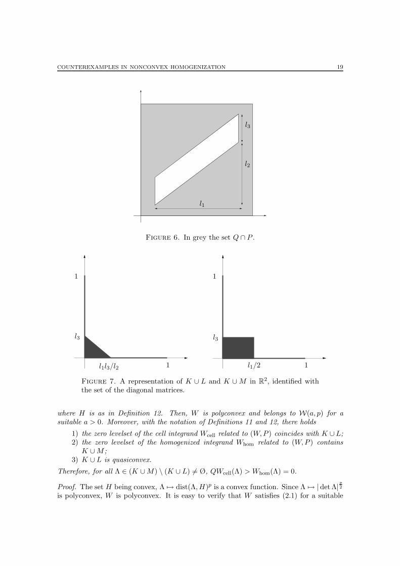
Geometry and energyLet us begin by describing the geometry of the subset P , sketched on Figure 6.
Definition 11. The set P is the complement in R2 of the set
⋃m∈Z2 O +m, where
O :=x ∈ Q : x1 ∈ [1/8, 7/8] and 3x1 ≤ 4x2 ≤ 3x1 + 1
.
Let us introduce some sets in the space M2, that we will use to describe the energy
density.
Definition 12. Let l1 := 3/4, l2 := 9/16 and l3 := 1/4. We consider the following sets(see Figure 7):
• K1 :=diag(s, 0) : s ∈ (0, 1]
and K2 :=
diag(0, t) : t ∈ (0, 1]
;
• K := K1 ∪K2 ∪ diag(0, 0);• H :=
diag(s, t) : s, t ∈ [0, 1] and t ≤ 1 − s
;
• L :=diag(s, t) : 0 < s ≤ l1l3/l2 and 0 < t ≤ l3 − l2s/l1
;
• M :=diag(s, t) : 0 < s ≤ l1/2 and 0 < t ≤ l3
.
The counterexample is as follows.
Theorem 6. Let p ∈ [2,+∞) and let W : M2 → [0,+∞) be given by
W (Λ) := dist(Λ,H)p + |det(Λ)|p
2 ,
COUNTEREXAMPLES IN NONCONVEX HOMOGENIZATION 19
l3
l2
l1
Figure 6. In grey the set Q ∩ P .
l3
l1l3/l2
1
1
l3
l1/2
1
1
Figure 7. A representation of K ∪ L and K ∪M in R2, identified with
the set of the diagonal matrices.
where H is as in Definition 12. Then, W is polyconvex and belongs to W(a, p) for asuitable a > 0. Moreover, with the notation of Definitions 11 and 12, there holds
1) the zero levelset of the cell integrand Wcell related to (W,P ) coincides with K ∪L;2) the zero levelset of the homogenized integrand Whom related to (W,P ) contains
K ∪M ;3) K ∪ L is quasiconvex.
Therefore, for all Λ ∈ (K ∪M) \ (K ∪ L) 6= Ø, QWcell(Λ) > Whom(Λ) = 0.
Proof. The set H being convex, Λ 7→ dist(Λ,H)p is a convex function. Since Λ 7→ |det Λ| p
2
is polyconvex, W is polyconvex. It is easy to verify that W satisfies (2.1) for a suitable

20 M. BARCHIESI & A. GLORIA
a > 0. The strict inequality QWcell(Λ) > Whom(Λ) is a direct consequence of 1)-3) usingLemma 5. Let us split the proof of 1)-3) into three steps.
Step 1. Since W−1(0) = K, by using φ ≡ 0 as a test function in (2.2), we obtainK ⊆W−1
cell(0). Let us check that L ⊆W−1cell(0). Given s ∈ (0, l1l3/l2) and t ∈ (0, l3− l2s/l1),
we define ψ : Q→ R2 by
ψ(1)(x) :=
0 if x ∈ (0, 1/2) × (0, 1)
x1 − 1/2 if x ∈ [1/2, 1/2 + s] × (0, 1)
s if x ∈ (1/2 + s, 1) × (0, 1)
;
ψ(2)(x) :=
0 if x ∈ (0, 1) × (0, 5/8 − t)
x2 − 5/8 + t if x ∈ (0, 1) × [5/8 − t, 5/8]
t if x ∈ (0, 1) × (5/8, 1)
.
(4.1)
We have that φ(x) := ψ(x) − diag(s, t) · x is Q-periodic and that ∇ψ(x) ∈ K if x ∈ P .More precisely, ∇ψ(x) /∈ K only if x belongs to [1/2, 1/2 + s]× [5/8− t, 5/8] ⊆ O. There,∇ψ ≡ diag(1, 1) (see Figures 8 and 9).
1/2
Figure 8. The first component of ψ is flat on Q ∩ P with the exceptionof the grey zone, where the gradient is equal to (1, 0).
It remains to proceed with the delicate part of the argument: the opposite inclusionW−1
cell(0) ⊆ K∪L. Let C = (cij) ∈W−1cell(0). By Lemma 7, there exists a Lipschitz function
ψ : Q → R2 such that ∇ψ(x) ∈ K for L2a.e. x ∈ Q ∩ P and φ(x) := ψ(x) − C · x is
Q-periodic. We will show that ψ is substantially a laminate as in (4.1). Let us point outthat if Λ ∈ K, then either Λ11 = 0 or Λ22 = 0.
We use the following notation:
Ls :=r ∈ (0, 1) : (s, r) ∈ (s × (0, 1)) ∩ P
;
Ls :=r ∈ (0, 1) : (r, s) ∈ ((0, 1) × s) ∩ P
.
Notice that Ls = (0, 1) if s ∈ (0, 1/8)∪(7/8, 1) and that Ls has two connected componentsif s ∈ [1/8, 7/8]. Similarly, Ls = (0, 1) if s ∈ (0, 3/32)∪(29/32, 1) and it has two connectedcomponents if s ∈ [3/32, 29/32].

COUNTEREXAMPLES IN NONCONVEX HOMOGENIZATION 21
5/8
Figure 9. The second component of ψ is flat on Q∩P with the exceptionof the grey zone, where the gradient is equal to (0, 1).
Since ∂2ψ(1)(x) = 0 for L2a.e. x ∈ Q ∩ P , ψ(1)(s, ·) is constant along any connected
component of Ls for all s ∈ (0, 1). In particular for s ∈ (0, 1/8) ∪ (7/8, 1), ψ(1)(s, ·)is constant and therefore the (0, 1)-periodicity of φ(s, ·) imposes that c12 = 0. For s ∈[1/8, 7/8], ψ(1)(s, ·) is constant on each of the two connected components of Ls. Hence,
by periodicity, ψ(1)(s, ·) is constant on the whole Ls.From the fact that ψ(1)(s, ·) is constant along Ls for any s ∈ (0, 1), we can deduce that
if x ∈ Q∩P is a differentiability point for ψ(1), then ψ(1) is differentiable in all x1×Lx1
and∇ψ(1)(x) = ∇ψ(1)(x) ∀x ∈ x1 × Lx1 . (4.2)
Similarly, one can show that c21 = 0 and that if x ∈ Q ∩ P is a differentiability pointfor ψ(2), then ψ(2) is differentiable in all Lx2
× x2 and
∇ψ(2)(x) = ∇ψ(2)(x) ∀x ∈ Lx2 × x2. (4.3)
Let X1, X2 be two L1-negligible subsets of the interval (0, 1) such that ψ is differentiable
in P := (Q ∩ P ) \ (X1 ×X2) and ∇ψ(x) ∈ K for all x ∈ P . Let us show that, if for some
x ∈ P there holds ∇ψ(x) ∈ K1, then
∇ψ(x) ∈ K1 ∪ diag(0, 0) ∀x ∈ P ∩((0, 1) × Lx1
). (4.4)
In fact, since ∇ψ(1)(x) 6= (0, 0), we have ∇ψ(1) 6= (0, 0) in x1 × Lx1 due to (4.2) and
therefore ∇ψ ∈ K1 in x1 ×(Lx1 \ X2
). As now ∇ψ(2) ≡ (0, 0) in x1 ×
(Lx1 \ X2
),
(4.3) implies that ∇ψ(2) ≡ (0, 0) in P ∩((0, 1) × Lx1
).
We are in position to conclude the first step. Given s ∈ (0, 1/8) \X1 and t ∈ (0, 3/32) \X2, we define the following two sets.
S : =s ∈ (0, 1) \X1 : ∂1ψ
(1)(s, t) > 0;
T : =t ∈ (0, 1) \X2 : ∂2ψ
(2)(s, t) > 0.
Since ∇ψ ∈ K, ∂1ψ(1)(s, t) ≤ 1 for all s ∈ S, and we infer from
c11 =
∫ 1
0c11 + ∂1φ
(1)(s, t)ds =
∫ 1
0∂1ψ
(1)(s, t)ds =
∫
S∂1ψ
(1)(s, t)ds,
22 M. BARCHIESI & A. GLORIA
that 0 ≤ c11 ≤ L1(S). Similarly, 0 ≤ c22 ≤ L1(T ). In particular this shows that
c11, c22 ∈ [0, 1].
If c11 > 0, for any ε > 0 there exist s1, s2 ∈ S such that s2 − s1 ≥ c11 − ε. Recallingthat if ∇ψ(x) ∈ K and ∂1ψ
(1)(x) > 0 then ∇ψ(x) ∈ K1, from (4.4), we obtain
∇ψ(x) ∈ K1 ∪ diag(0, 0) ∀x ∈ P ∩((0, 1) × (Ls1 ∪ Ls2)
).
Since T ⊆ (0, 1) \ (Ls1 ∪ Ls2), we have the estimate
c22 ≤ L1(T ) ≤ max
0,l2l1
(s1 − s2) + l3
≤ max
0,l2l1
(−c11 + ε) + l3
.
The arbitrariness of ε > 0 completes the proof of the step.
Step 2. Since Whom is rank-one convex and W−1hom(0) ⊇ K, it is sufficient to prove that
C := diag(l1/2, l3) ∈W−1hom(0).
Let us construct a Lipschitz function ψ : Q2 → R2 such that ∇ψ ∈ K a.e. in Q2 ∩ P and
φ(x) := ψ(x) − C · x is Q2-periodic. In this way we get
Whom(C) ≤ 1
4
∫
Q2∩PW(C + ∇φ(x)
)dx = 0.
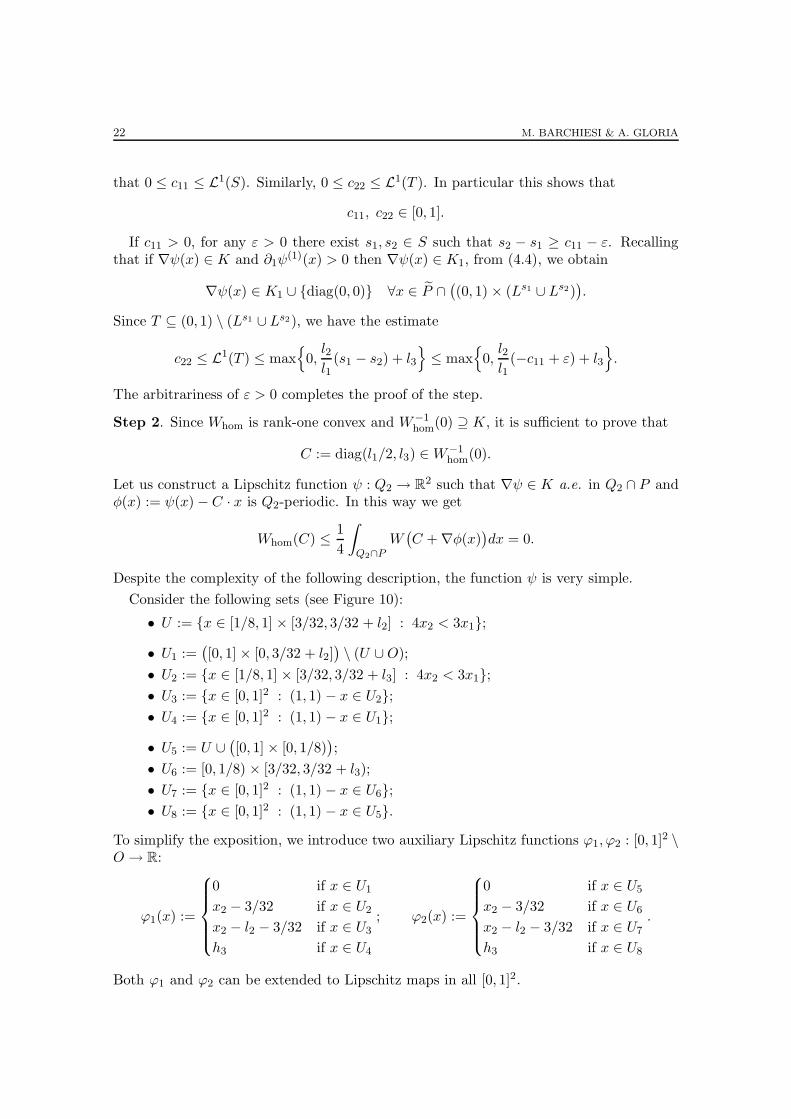
Despite the complexity of the following description, the function ψ is very simple.
Consider the following sets (see Figure 10):
• U := x ∈ [1/8, 1] × [3/32, 3/32 + l2] : 4x2 < 3x1;
• U1 :=([0, 1] × [0, 3/32 + l2]
)\ (U ∪O);
• U2 := x ∈ [1/8, 1] × [3/32, 3/32 + l3] : 4x2 < 3x1;• U3 := x ∈ [0, 1]2 : (1, 1) − x ∈ U2;• U4 := x ∈ [0, 1]2 : (1, 1) − x ∈ U1;
• U5 := U ∪([0, 1] × [0, 1/8)
);
• U6 := [0, 1/8) × [3/32, 3/32 + l3);
• U7 := x ∈ [0, 1]2 : (1, 1) − x ∈ U6;• U8 := x ∈ [0, 1]2 : (1, 1) − x ∈ U5.
To simplify the exposition, we introduce two auxiliary Lipschitz functions ϕ1, ϕ2 : [0, 1]2 \O → R:
ϕ1(x) :=
0 if x ∈ U1
x2 − 3/32 if x ∈ U2
x2 − l2 − 3/32 if x ∈ U3
h3 if x ∈ U4
; ϕ2(x) :=
0 if x ∈ U5
x2 − 3/32 if x ∈ U6
x2 − l2 − 3/32 if x ∈ U7
h3 if x ∈ U8
.
Both ϕ1 and ϕ2 can be extended to Lipschitz maps in all [0, 1]2.
COUNTEREXAMPLES IN NONCONVEX HOMOGENIZATION 23
U1
U2
U3
U4
332
l2 + 332
l3 + 332
U5U6
U7U8
Figure 10
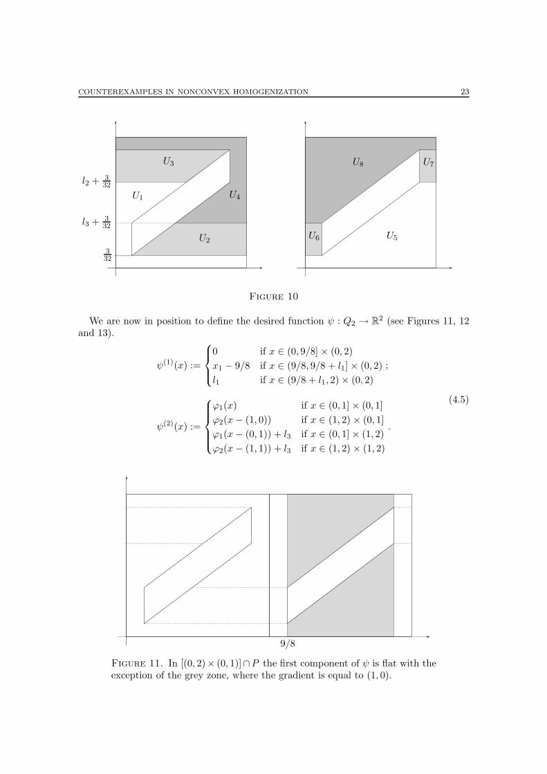
We are now in position to define the desired function ψ : Q2 → R2 (see Figures 11, 12
and 13).
ψ(1)(x) :=
0 if x ∈ (0, 9/8] × (0, 2)
x1 − 9/8 if x ∈ (9/8, 9/8 + l1] × (0, 2)
l1 if x ∈ (9/8 + l1, 2) × (0, 2)
;
ψ(2)(x) :=
ϕ1(x) if x ∈ (0, 1] × (0, 1]
ϕ2(x− (1, 0)) if x ∈ (1, 2) × (0, 1]
ϕ1(x− (0, 1)) + l3 if x ∈ (0, 1] × (1, 2)
ϕ2(x− (1, 1)) + l3 if x ∈ (1, 2) × (1, 2)
.
(4.5)
9/8
Figure 11. In [(0, 2)× (0, 1)]∩P the first component of ψ is flat with theexception of the grey zone, where the gradient is equal to (1, 0).
24 M. BARCHIESI & A. GLORIA
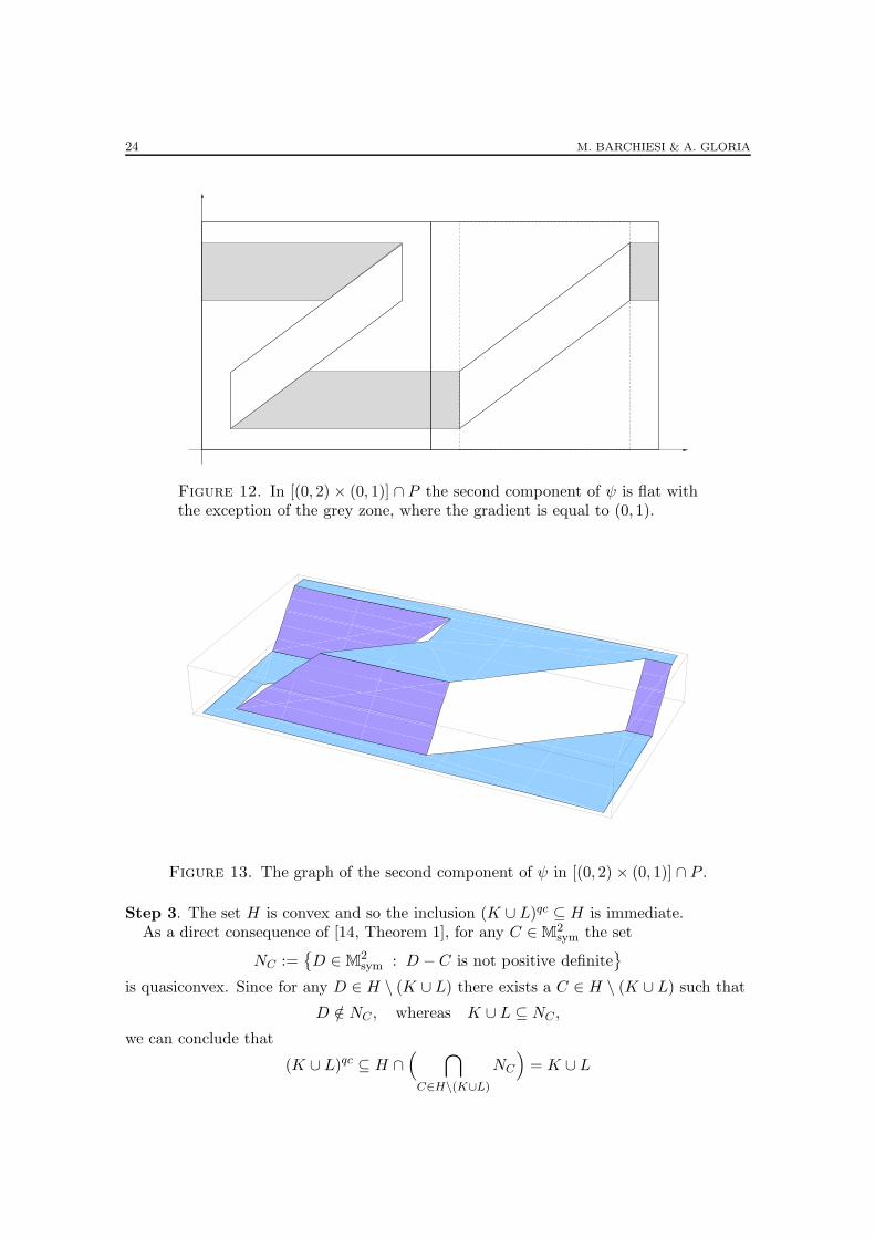
Figure 12. In [(0, 2) × (0, 1)] ∩ P the second component of ψ is flat withthe exception of the grey zone, where the gradient is equal to (0, 1).
Figure 13. The graph of the second component of ψ in [(0, 2) × (0, 1)] ∩ P .
Step 3. The set H is convex and so the inclusion (K ∪ L)qc ⊆ H is immediate.As a direct consequence of [14, Theorem 1], for any C ∈ M
2sym the set
NC :=D ∈ M
2sym : D − C is not positive definite
is quasiconvex. Since for any D ∈ H \ (K ∪ L) there exists a C ∈ H \ (K ∪ L) such that
D /∈ NC , whereas K ∪ L ⊆ NC ,
we can conclude that
(K ∪ L)qc ⊆ H ∩( ⋂
C∈H\(K∪L)
NC
)= K ∪ L

COUNTEREXAMPLES IN NONCONVEX HOMOGENIZATION 25
and then K ∪ L is quasiconvex.
Remark 5. The proof of Theorem 6 does not take advantage of the particular structureof W but it is based only on the fact that W−1(0) = K. Therefore, instead of W wecan consider the function V : M
2 → [0,+∞) defined as the quasiconvex envelope ofdist(·,K)p, p ∈ (1,+∞). Indeed, since K is polyconvex (because zero levelset of thepolyconvex function W ), by Lemma 5 it follows that V −1(0) = K. Note that in this wayour counterexample covers also the case of energy densities with growth p ∈ (1, 2).
Remark 6. LetN be a convex and compact subset of M2 sufficiently large so that ∇ψ ∈ N
a.e. inQ2, where ψ is defined as in (4.5). Consider now the function V : R2×M
2 → [0,+∞)defined by
V (x,Λ) := χP (x)W (Λ) + (1 − χP (x))dist(Λ, N)p.
Since Wcell ≤ Vcell, we have the inclusion V −1cell (0) ⊆ K ∪ L. We also have the inclusion
K ∪M ⊆ V −1hom(0): in fact K ⊆ V −1
hom(0) (because K ⊆ N) and diag(h1/2, h3) ∈ V −1hom(0)
(by using again ψ). In this way we can conclude that also by mixing a polyconvex functionand a convex function, the inequality QVcell > Vhom can occur.
Appendix: Stefan Muller’s example in dimension three
To show that Proposition 1 is not peculiar to dimension two, let us consider the corre-sponding energy for a three-dimensional soft material reinforced by a strong plate. Theenergy is now given by W0 : M
3 ∋ Λ 7→ |Λ|4 + f(detΛ) where
f(z) :=
12(1 + a)2
z + a− 12(1 + a) − 9 if z > 0
12(1 + a)2
a− 12(1 + a) − 9 − 12(1 + a)2
a2z if z ≤ 0
for a ∈ (0, 1/2). The energy density under consideration is still of the formW η : R3×M
3 →[0,+∞), (y,Λ) 7→ χη(y)W0(Λ) where χη is the Q-periodic extension on R
3 of
χη(y) :=
1 if y1 ∈ (0, 1/2)
η if y1 ∈ [1/2, 1),
with Q = (0, 1)3 ∋ y = (y1, y2, y3) and η > 0. Such an energy density is nonnegative,polyconvex, frame-invariant and its zero-levelset is SO3.
Proposition 2. For all λ1, λ2 ∈ (0, 1), there exists c > 0 independent of η such that
QW ηcell(Λ) ≤ η c,
where Λ := diag(1, λ1, λ2).
Proof. Essentially, one has to construct a Lipschitz domain U of R3, a function φ ∈
W 1,∞per (U,R3) and a function ϕ ∈ L∞(U,W 1,∞
per (Q,R3)) such that Λ+∇φ(x)+∇yϕ(x, y) ∈SO3 for all x ∈ U and y ∈ (0, 1/2) × (0, 1)2 (the strong phase of the material).
Notation. The canonical basis of R3 is denoted by e1, e2, e3.

26 M. BARCHIESI & A. GLORIA
We will use the angles θ and γ defined by
cos θ = λ1, sin θ =√
1 − λ21,
cos γ = λ2, sin γ =√
1 − λ22.
We set ρ :=√
sin2 θ + cos2 θ sin2 γ and define the unit vectors e4 and e5 by
e4 :=1
ρ(sin θ e2 + cos θ sin γ e3) ,
e5 :=1
ρ(sin θ e2 − cos θ sin γ e3) .
Definition of U . In order to describe U , we need the following quantity
τ :=cos θ sin γ
sin θ.
We set U := U1 ∪ U2 ∪ U3 ∪ U4, where
U1 :=(x1, x2, x3) : 0 < x1 < 1; 0 < x3 ≤ 1/2; 1/2 − τx3 ≤ x2 < 1 − τx3
,
U2 :=(x1, x2, x3) : 0 < x1 < 1; 0 < x3 ≤ 1/2; −τx3 < x2 ≤ 1/2 − τx3
,
U3 :=(x1, x2, x3) : 0 < x1 < 1; 1/2 ≤ x3 < 1; 1/2 − τ(1 − x3) ≤ x2 < 1 − τ(1 − x3)
,
U4 :=(x1, x2, x3) : 0 < x1 < 1; 1/2 ≤ x3 < 1; −τ(1 − x3) < x2 ≤ 1/2 − τ(1 − x3)
.
The domains U1, U2, U3, U4 are sketched on Figure 14. Note that the interface between U1
and U2 (resp. U3 and U4) is perpendicular to e4 (resp. e5).
Zone U1: A1 Zone U3: A3
Zone U2: A2 Zone U4: A4
x2
x3
Figure 14. Domain U (in the plane generated by e2, e3).
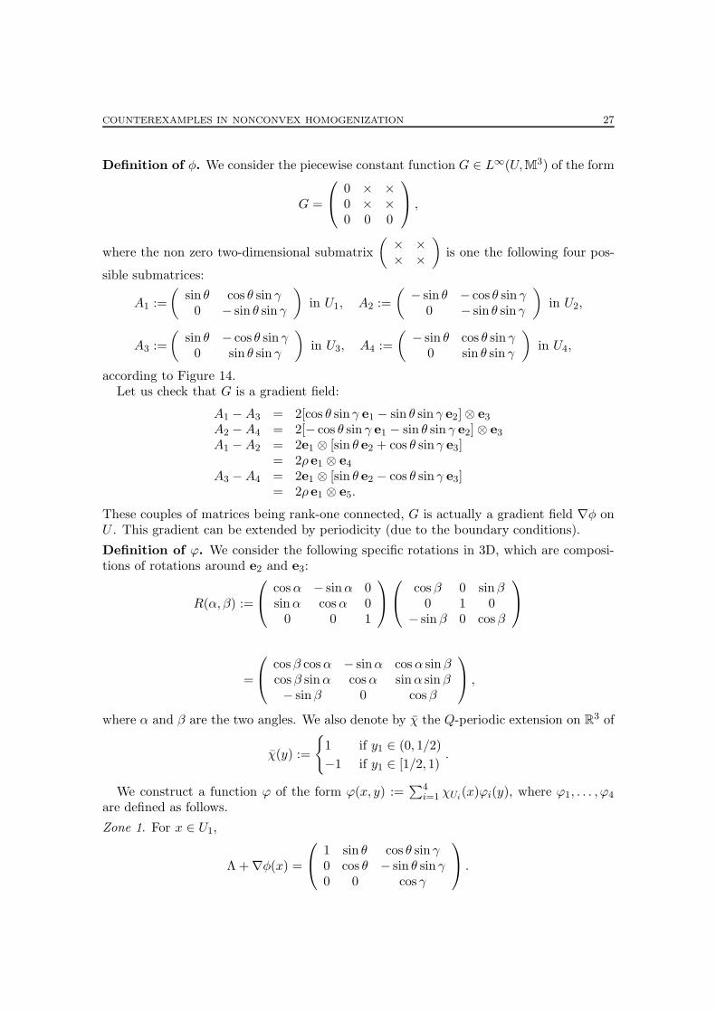
COUNTEREXAMPLES IN NONCONVEX HOMOGENIZATION 27
Definition of φ. We consider the piecewise constant function G ∈ L∞(U,M3) of the form
G =
0 × ×0 × ×0 0 0
,
where the non zero two-dimensional submatrix
(× ×× ×
)is one the following four pos-
sible submatrices:
A1 :=
(sin θ cos θ sin γ
0 − sin θ sin γ
)in U1, A2 :=
(− sin θ − cos θ sin γ
0 − sin θ sin γ
)in U2,
A3 :=
(sin θ − cos θ sin γ
0 sin θ sin γ
)in U3, A4 :=
(− sin θ cos θ sin γ
0 sin θ sin γ
)in U4,
according to Figure 14.Let us check that G is a gradient field:
A1 −A3 = 2[cos θ sin γ e1 − sin θ sin γ e2] ⊗ e3
A2 −A4 = 2[− cos θ sin γ e1 − sin θ sin γ e2] ⊗ e3
A1 −A2 = 2e1 ⊗ [sin θ e2 + cos θ sin γ e3]= 2ρ e1 ⊗ e4
A3 −A4 = 2e1 ⊗ [sin θ e2 − cos θ sin γ e3]= 2ρ e1 ⊗ e5.
These couples of matrices being rank-one connected, G is actually a gradient field ∇φ onU . This gradient can be extended by periodicity (due to the boundary conditions).
Definition of ϕ. We consider the following specific rotations in 3D, which are composi-tions of rotations around e2 and e3:
R(α, β) :=
cosα − sinα 0sinα cosα 0
0 0 1
cos β 0 sinβ0 1 0
− sin β 0 cosβ
=
cos β cosα − sinα cosα sin βcos β sinα cosα sinα sin β− sin β 0 cos β
,
where α and β are the two angles. We also denote by χ the Q-periodic extension on R3 of
χ(y) :=
1 if y1 ∈ (0, 1/2)
−1 if y1 ∈ [1/2, 1).
We construct a function ϕ of the form ϕ(x, y) :=∑4
i=1 χUi(x)ϕi(y), where ϕ1, . . . , ϕ4
are defined as follows.
Zone 1. For x ∈ U1,
Λ + ∇φ(x) =
1 sin θ cos θ sin γ0 cos θ − sin θ sin γ0 0 cos γ
.

28 M. BARCHIESI & A. GLORIA
We then choose ϕ1 ∈W 1,∞per (Q,R3) such that
∇ϕ1(y) = χ(y)
cos γ cos θ − 1 0 0− cos γ sin θ 0 0
− sin γ 0 0
.
In the strong phase (χ(y) = 1),
Λ + ∇φ(x) + ∇ϕ1(y) =
cos γ cos θ sin θ cos θ sin γ− cos γ sin θ cos θ − sin θ sin γ
− sin γ 0 cos γ
= R(θ, γ)
is a rotation, with θ = −θ. In the soft phase (χ(y) = −1)
Λ + ∇φ(x) + ∇ϕ1(y) =
2 − cos γ cos θ − sin θ cos θ sin γ
− cos γ sin θ cos θ sin θ sin γsin γ 0 cos γ
.
Zone 2. For x ∈ U2,
Λ + ∇φ(x) =
1 − sin θ − cos θ sin γ0 cos θ − sin θ sin γ0 0 cos γ
.
We then choose ϕ2 ∈W 1,∞per (Q,R3) such that
∇ϕ2(y) = χ(y)
cos γ cos θ − 1 0 0cos γ sin θ 0 0
sin γ 0 0
.
In the strong phase (χ(y) = 1),
Λ + ∇φ(x) + ∇ϕ2(y) =
cos γ cos θ − sin θ − cos θ sin γcos γ sin θ cos θ − sin θ sin γ
sin γ 0 cos γ
= R(θ, γ)
is a rotation, with γ = −γ. In the soft phase (χ(y) = −1),
Λ + ∇φ(x) + ∇ϕ2(y) =
2 − cos γ cos θ − sin θ cos θ sin γ− cos γ sin θ cos θ sin θ sin γ
sin γ 0 cos γ
.
Zones 3 and 4. Proceeding as above, one may find ϕ3, ϕ4 ∈W 1,∞per (Q,R3) such that for all
x ∈ U3 and y ∈ (0, 1/2) × (0, 1)2,
Λ + ∇φ(x) + ∇ϕ3(y) =
cos γ cos θ sin θ − cos θ sin γ− cos γ sin θ cos θ sin θ sin γ
sin γ 0 cos γ
= R(θ, γ)
is a rotation, with θ = −θ, γ = −γ; and for all x ∈ U4 and y ∈ (0, 1/2) × (0, 1)2,
Λ + ∇φ(x) + ∇ϕ4(y) =
cos γ cos θ − sin θ cos θ sin γcos γ sin θ cos θ sin θ sin γ− sin γ 0 cos γ
= R(θ, γ)

COUNTEREXAMPLES IN NONCONVEX HOMOGENIZATION 29
is a rotation.
Finally, we are in position to conclude the proof. By using φ and ϕ defined above astest-functions, one obtains
QW ηcell(Λ) ≤
∫
U
∫
QW η(y,Λ + ∇φ(x) + ∇yϕ(x, y)
)dy dx ≤ η c,
where c = max(W (Ci))/2 and Cii is the finite set of values taken by Λ + ∇φ(x) +∇yϕ(x, y) in the soft phase.
Acknowledgments
M. Barchiesi wishes to thank Andrea Braides, Giovanni Leoni and Enzo Nesi for theiruseful comments and suggestions. A. Gloria gratefully thanks Andrea Braides and Ste-fan Muller for stimulating discussions. The research of M. Barchiesi was supported bythe Center for Nonlinear Analysis (NSF Grants No. DMS-0405343 and DMS-0635983).The research of A. Gloria was supported by the Hausdorff Center for Mathematics. Healso acknowledges the support from the Marie Curie Research Training Network MRTN-CT-2004-505226 ‘Multi-scale modelling and characterisation for phase transformations inadvanced materials’ (MULTIMAT).
References
[1] R. Alicandro and M. Cicalese. A general integral representation result for the continuum limits ofdiscrete energies with superlinear growth. SIAM J. Math. Anal., 36:1–37, 2004.
[2] R. Alicandro, M. Cicalese, and A. Gloria. Integral representation results for energies defined on sto-chastic lattices and application to nonlinear elasticity. In preparation.
[3] J.-F. Babadjian and M. Barchiesi. A variational approach to the local character of G-closure: theconvex case. Annales de l’institut Henri Poincare: Analyse non lineaire, 2008. To appear.
[4] J.M. Ball and R.D. James. Fine mixtures as minimizers of energy. Arch. Rat. Mech. Anal., 100:13–52,1987.
[5] J. M. Ball & R. D. James. Proposed experimental tests of a theory of fine microstructure and thetwo-well problem. Phil. Trans. Roy. Soc. London A, 338:389–450, 1992.
[6] M. Barchiesi. Loss of polyconvexity by homogenization: a new example. Calc. Var. Partial DifferentialEquations, 30:215–230, 2007.
[7] A. Braides and A. Defranceschi. Homogenization of Multiple Integrals, volume 12 of Oxford LectureSeries in Mathematics and Its Applications. Oxford University Press, 1998.
[8] B. Dacorogna. Direct methods in the calculus of variations, vol. 78 of Applied Mathematical Sciences.Springer, Berlin, 2nd ed., 2008.
[9] I. Fonseca & G. Leoni. Modern methods in the Calculus of Variations: Sobolev spaces. In preparation.[10] E. Giusti. Direct methods in the calculus of variations. World Scientific Publishing Co. Inc., River
Edge, NJ, 2003.[11] T. Iwaniec, G. Verchota & A. Vogel. The Failure of Rank-One Connections. Arch. Rational Mech.
Anal., 163:125–169, 2002.[12] S. Muller. Homogenization of nonconvex integral functionals and cellular elastic materials. Arch. Rat.
Anal. Mech., 99:189–212, 1987.[13] S. Muller. Variational models for microstructure and phase transitions. In Calculus of variations and
geometric evolution problems (Cetraro, 1996), volume 1713 of Lecture Notes in Math., pages 85–210.Springer, Berlin, 1999.
[14] V. Sverak. New examples of quasiconvex functions. Arch. Rational Mech. Anal., 119:293–300, 1992.[15] V. Sverak. On the problem of two wells. volume 54 of IMA Vol. Appl. Math., pages 183–189. Springer,
1993.

30 M. BARCHIESI & A. GLORIA
(Marco Barchiesi) CNA, Carnegie Mellon University, Pittsburgh, PA 15213, USA
E-mail address: [email protected]
(Antoine Gloria) IAM, Universitat Bonn, Wegelerstr. 10, 53115 Bonn, Germany
E-mail address: [email protected]