NBER WORKING PAPER SERIES

THE BEHAVIOR OF HOME BUYERS IN BOOM AND POST BOOM MARKETS

Karl E. Case

Robert J. Shiller

Working Paper No. 2748

NATIONAL BUREAU OF ECONOMIC RESEARCH1050 MassachusettS Avenue

Cambridge, MA 02138October 1988

The authors are indebted to the survey respondants who took valuable time to

complete the questionnaire. We also want to thank Alicia Munnell, Kenneth

Rosen, Jeremy Siegel and participants at the Sage Foundation Conference on

Behavioral Finance as well as seminar participants at Harvard and the

University of Pennsylvania for helpful discussions. We are also grateful to

Anne Kinsella at the Boston Federal Reserve Bank and Larry Baldwin at

Wellesley for masterful programming to help get the survey out and the

returns coded. Paula Andres, Jie Gao and Janet Hanousek worked very hard as

research assistants. The research reported here is part of the NBER'sprogram on Financial Markets and Monetary Economics. Funding was provided by

the Federal Reserve Bank of Boston, the National Science Foundation, andWellesley College. Any opinions expressed here are those of the authors and

not of the National Bureau of Economic Research or the supporting agencies.

NBER Working Paper #2748October 1988

THE BEHAVIOR OF HOME BUYERS IN BOOM AND POST BOOM MARKETS

ABSTRI

A questionnaire survey looked at home buyers in May 1988 in

two "boom" cities currently experiencing rapid price increases

(Anaheim and San Francisco), a "post—boom" city whose home prices

are stable or falling a couple years after rapid price increase

(Boston) and a "control" city where home prices had been very

stable (Milwaukee).

Home buyers in the boom cities had much higher expectations

for future price increases, and were more influenced by

investment motives. The interpretations that people place on

the boom are not usually related to any concrete news event;

there are instead oft-repeated cliches about home prices. This

suggests that sudden real estate booms have, at least in part, a

social, rather than rational or economic, basis.

There is evidence for excess demand in boom markets and

excess supply in the post-boom market; there appear to be various

reasons for this: notions of fairness, intrinsic worth, popular

theories about prices, coordination problems, and simple

mistakes.

Karl E. Case Robert 3. Shiller

Department of Economics Cowles Foundation

Wellesley College Yale University

Wellesley, MA 02181 Box 2125 Yale StationNew Haven, CT 06520

The Behavior of Home Buyers In Boom and Post—Boom Markets

Karl E. Case and Robert 3. Shlller*

A recent development In the United States market for single—family homes

has provided an ideal laboratory in which to study the sources of volatility

in home prices: prices have been moving In dramatically different ways at the

same time in different parts of the country. A boom in housing prices has

appeared in California, with price increases from late 1987 to mid—1988

exceeding 20 percent in many cities. At the very same time, a post—boom

market exists in the Northeast. A remarkable boom occurred between 1983 and

mid—1987 in many places from New York to Boston, where housing prices more

than doubled in those three and one—half years. That boom appears to be over,

with prices actually falling in late 1987. At the same time, it Is possible

to observe a housing market in the Midwest that has had no sign of a boom for

the past five years.

We exploited this opportunity by collecting data about the behavior of

home buyers in these different markets using questionnaire survey methods.

Identical questionnaires were sent to those who bought homes in May of 1988 in

each of four markets: Anaheim (Orange County) and San Francisco, California

(two "boom" markets); Boston, Massachusetts (a "post—boom" market); and

Milwaukee, Wisconsin (a t;contro1I sample, representing more normal housing

market conditions). Since the questionnaires were identical and were sent out

at the same time, differences in answers across cities can be attributed only

to differences In the local market for housing and not to differences in the

wording or order of questions or to national economic conditions.

He sought information that would help answer some nagging questions about

the nature and causes of booms in housing markets. Most fundamentally, what

—2-.

causes sudden and often dramatic and sustained price movements? Although

questionnaire survey methods can never provide a definitive answer to such a

question, they can provide information that helps us begin to understand the

process: What are home buyers thinking about, and what sources of information

are used to decide how much to pay for a house? How motivated are they by

investment considerations, and how do they assess investment potential? Is

destabilizing speculation affecting housing prices?

Second, why does a state of excess demand tend to occur in boom markets,

where some people reportedly stand In line to make offers on the day that a

house Is listed for sale, often making bids that are above the asking price?

Why don't sellers just increase their asking prices until the excess demand

disappears?

Third, why does a state of excess supply seem to occur in post—boom

markets, where people reportedly take substantial periods of time to sell

their homes? Why don't people just cut their asking prices to eliminate the

excess supply?

Housing price booms have raised a number of concerns. A boom In housing

prices represents a major redistribution of wealth. Those who own see their

equity increase while those who do not face higher rents and reduced

probability of owning. This redistribution seems capricious and unfair to

many. Some have also expressed concern that high housing prices have made it

more difficult for firms to attract labor to the boom regions. A special

report In the Harvard Business Review spoke of a "convulsion In U.S. housing"

that has begun to affect American business.1 The report cites examples of

firms In Boston and New York that have experienced severe problems

recruiting. Many have chosen to relocate outside the region as a result.

Others are concerned that If speculators are pushing housing prices up

temporarily, then housing prices may fall rapidly, creating turmoil among

—3—

homeowners and homebuilders and in the banking system. On August 22, 1988,

the front page of Barron's contained a full—page sketch of a home falling off

a cliff with the headline "The Coming Collapse of Home Prices." A few cities

in recent years have In fact witnessed falling home prices. The best known

example Is Houston, where the median price of existing single—family homes

dropped 24 percent in two years, contributing to the Insolvency of large

savings and loan institutions and multi—billion—dollar payouts by the Federal

Savings and Loan Insurance Corporation.

Given the seriousness of the problems associated with rising and falling

housing prices, surprisingly little research has been done on the questions we

pose here. Most models of housing price movements have focused on

macroeconomic variables such as interest rates, Income, and national

demographic trends. But the simple fact that the most dramatic examples of

price booms have taken place in well—defined geographic areas while prices

were not rising in most of the country suggests that macro variables offer

only a partial explanation.

The causes of these booms are still not understood. A study by one of us

suggests that housing booms cannot be attributed to rational fundamental

factors. In a 1986 article in this Review, Case sought to explain the Boston

experience using data on economic fundamentals. His model included such

demand—side and supply—side variables as population growth, employment growth,

Interest rates (short—term and long—term), construction costs, Income growth,

tax rates, and the like. Estimated with data from 10 citIes over a 10—year

period, that model failed to explain more than a fraction of the observed

Increase in Boston housing prices. Case then put forward a conjecture that

the boom was essentially driven by expectations.

Part I of this paper describes the behavior of prices in the four

metropolitan areas surveyed. Part II describes the survey, Including samples

—4—

and response rates for each city. Part III summarizes the results of the

survey, and part IV presents some interpretations and conjectures.

I. Housing Prices in Four Metropolitan Areas

The survey described in Section II was sent to people who bought homes or

condominiums during the month of May 1988. By selecting buyers from a narrow

time window, we sought to control for national macroeconomic factors such as

interest rates and national income growth. Four metropolitan areas were

targeted for the survey. The four were chosen because of what we perceived to

be dramatic differences in recent price behavior.

Table 1 presents National Association of Realtors data on the median price

of existing single—family homes in each metropolitan area quarterly since 1983

and table 2 shows annual price increases. Chart 1 plots indexes derived from

table 1 for the same time period. Although we have shown in earlier work

(Case and Shiller 1987) that these are less than perfect measures of

appreciation, they are the only source consistent enough to allow such a

cross—cl ty comparison.

Orange County and San Francisco

The experience of these two very different California metropolitan areas

has been similar. Both experienced a period of rapid Increases In home prices

during the late 1970s. That came to an end in 1981. Beginning in late 1984,

prices began rising again In San Francisco; Orange County picked up in late

1986. WhIle prices In Boston were cooling in 1987 and 1988, San Francisco and

Orange County began booming. Table 3 and chart 2 show the pattern in Orange

County, and table 3 gives annual figures for several other areas in California

as well.

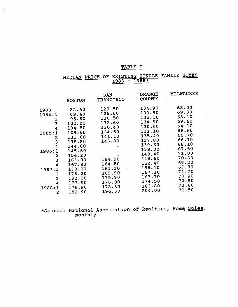
TABLE I

MEDIAN PRICE OF EXISTING SINGLE FAMILY HOMES1983 — 1988*

*Source: Nationalmonthly

Association of Realtors, Home Sales,

COUNTYBOSTON FRANCISCO

1983 82.60 129.50 134.90133.50

68.0069.80

1984:1 89.40 126.60135.10 68.10

2 95.60 130.50134.90 69.60

3 102.00 132.60130.60 64.10

4 104.80 130.40132.10 66.601885:1 108.60 134.50135.40 66.70

2 131.00 141.10137.80 66.70

3 138.80 143.80139.60 68.10

4 144.80 .138.00 67.601986:1 145.60 .149.40 71.00

2 156.20 .149.60 70.80

3 163.00 164.90152.40 69.20

4 167.80 164.80156.10 67.801987:1 170.00 161.30167.30 71.70

2 176.20 169.90167.70 70.90

3 182.20 175.90174.50 70.80

4 177.50 176.00183.80 72.601988:1 176.90 178.80

71.50

TABLE 2

ANNUAL INCREASES IN MEDIAN SINGLE FAMILY HOME PRICES1983 —1988*(percent)

1983—84 1984—85 1985—86 1986—87 1987—88

Boston 15.7 37.0 19.2 12.8 3.8

San Francisco 0.8 8.1 8.5** l1.0** 15.5

Orange County 0.1 0.2 10.3 12.0 21.9

Milwaukee 0.0 —2.2 6.6 1.0 —0.3

*Source: National Association of Realtors. Calculations donefrom Table 1. All changes are from second quarter to secondquarter except the change for 1983-84 which is the changefrom the 1983 annual figure to the 1984 second quarterfigure.**Figures for San Francisco were not available for the secondquarter of 1986; the changes presented are estimates.

0 q II I..) 0) 0 -o C

0.9

0 B

osto

n +

San

Fro

n Quarters

OrangeCo

Milw

auke

e

FIG

UR

E

1

IND

EX

ES

OF

M

ED

IAN

E

XIS

TIN

G S

ING

LE F

AM

ILY

HO

ME

S,

1983

—88

P

RIC

E

OF

2.4

2.3

2.2

2.1 2

1.9

1.8

1.7

1.6

1.5

1.4

1.3

1.2

1.1

83

851

861

871

881

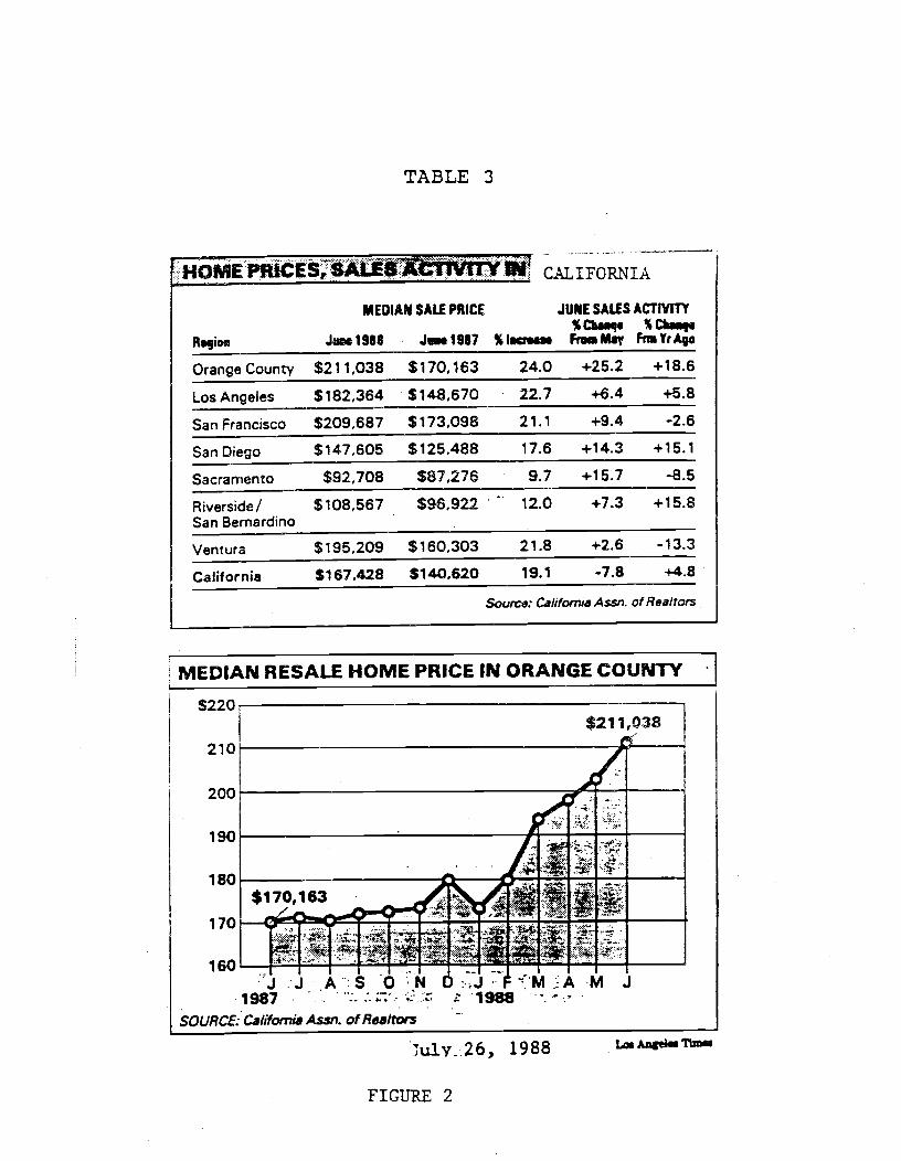
TABLE 3

IIOMEPRICES,SALE j! cipoiMEDIAN SALE PRICE JUNE SALES ACTIVITY

%haaq. %ta.q.Fm.May FnYrAeR.qioa Ja.19U J1987 SI.cs.us

Orange County $211,038 $170,163 24.0 +25.2 +18.6

Los Angeles $182,364 $148,670 22.7 4-6.4 +5.8

San Francisco $209,687 $173,098 21.1 +9.4 -2.6

San Diego $147,605 $125,488 17.6 +14.3 +15.1

Sacramento $92,708 $87,276 9.7 +15.7 -8.5

Riverside! $108,567$96,922 . -

.12.0 +7.3 +15.8

San Bernardino

Ventura $195,209 $160,303 21.8 +2.6 -13.3

California $167,428 $140,620 19.1 -7.8 +4.8

Source: California As.sn. of Realtors

MEDIAN RESALE HOME PRICE IN ORANGE COUNTY

:::

:_.

11

.

itiI41

.:

.. !-'..-,-

:. -__•.

u1y;.26, 1988

FIGURE 2

Lcs AngeMs

S220$21 If 038

21C

160 , , .1 ..i'J:J AS 0-N I1987 . 1988

SOURCE: California Assn. of Rca/tots

—5—

The height of the boom seems to have come In May 1988. Between May and

June, a single month, the California Association of Realtors reported a 10.2

percent increase in the median price of single—family homes In San Francisco

and a 4.1 percent increase in Orange County. Such rates of Increase drew

national attention. On June 1, 1988, the Hall Street Journal carried a

headline on the front page reading "Buyers' Panic Sweeps California's Big

Market in One—Family Homes." The Journal article speaks of "a buying frenzy

that extends to every segment of the market" and describes lines of 150 cars

waiting to buy houses. Articles on the real estate market appeared in the 1Q1

Angeles Times and the San Francisco Chronicle an average of more than four

times per week during the summer of 1988, carrying leads such as "The real

estate market is getting so frenzied, prospective home owners are offering

more than asking price" (Chronicle, 7/6/88). The president of the Alameda

County Board of Realtors is quoted in the same article: "The market is hotter

than a pistol . . .. I went to a presentation last night In Fremont for a

$400,000 home that had been on the market for five days. There were five

offers, and the winning bid was more than the asking price."

Boston

The Boston housing price boom began in 1983. The most rapid growth

occurred between 1984 and 1985 when growth rates neared 40 percent per year.

Multiple sales data presented In Case (1986) confirmed rapid acceleration of

prices beginning In the first quarter of 1984, peaking In the third quarter of

1985, and slowing steadily through 1986 and 1987. Housing prices doubled

between the beginning of 1984 and mid—1987.

Median price fell in Boston in both the fourth quarter of 1987 and the

first quarter of 1988. The Boston Globe reported the dip with great fanfare.

—6—

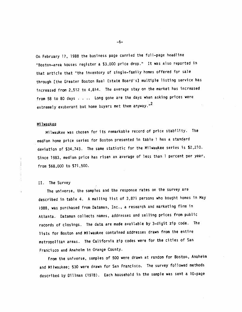
On February 17, 1988 the business page carried the full—page headline

"Boston—area houses register a $3,000 price drop." It was also reported In

that article that "the Inventory of single—family homes offered for sale

through [the Greater Boston Real Estate Board's) multiple listing service has

increased from 2,512 to 4,814. The average stay on the market has increased

from 58 to 80 days . . .. Long gone are the days when asking prices were

extremely exuberant but home buyers met them anyway."2

Milwaukee

Milwaukee was chosen for its remarkable record of price stability. The

median home price series for Boston presented In table 1 has a standard

deviation of $34,743. The same statistic for the Milwaukee series is $2,210.

Since 1983, median price has risen an average of less than 1 percent per year,

from $68,000 to $71,500.

II. The Survey

The universe, the samples and the response rates on the survey are

described in table 4. A mailing list of 3,871 persons who bought homes In May

1988, was purchased from Dataman, Inc., a research and marketing firm in

Atlanta. Dataman collects names, addresses and selling prices from public

records of closings. The data are made available by 3—digit zip code. The

lists for Boston and Milwaukee contained addresses drawn from the entire

metropolitan areas. The California zip codes were for the cities of San

Francisco and Anaheim in Orange County.

From the universe, samples of 500 were drawn at random for Boston, Anaheim

and Milwaukee; 530 were drawn for San Francisco. The survey followed methods

described by Dillman (1978). Each household In the sample was sent a 10—page

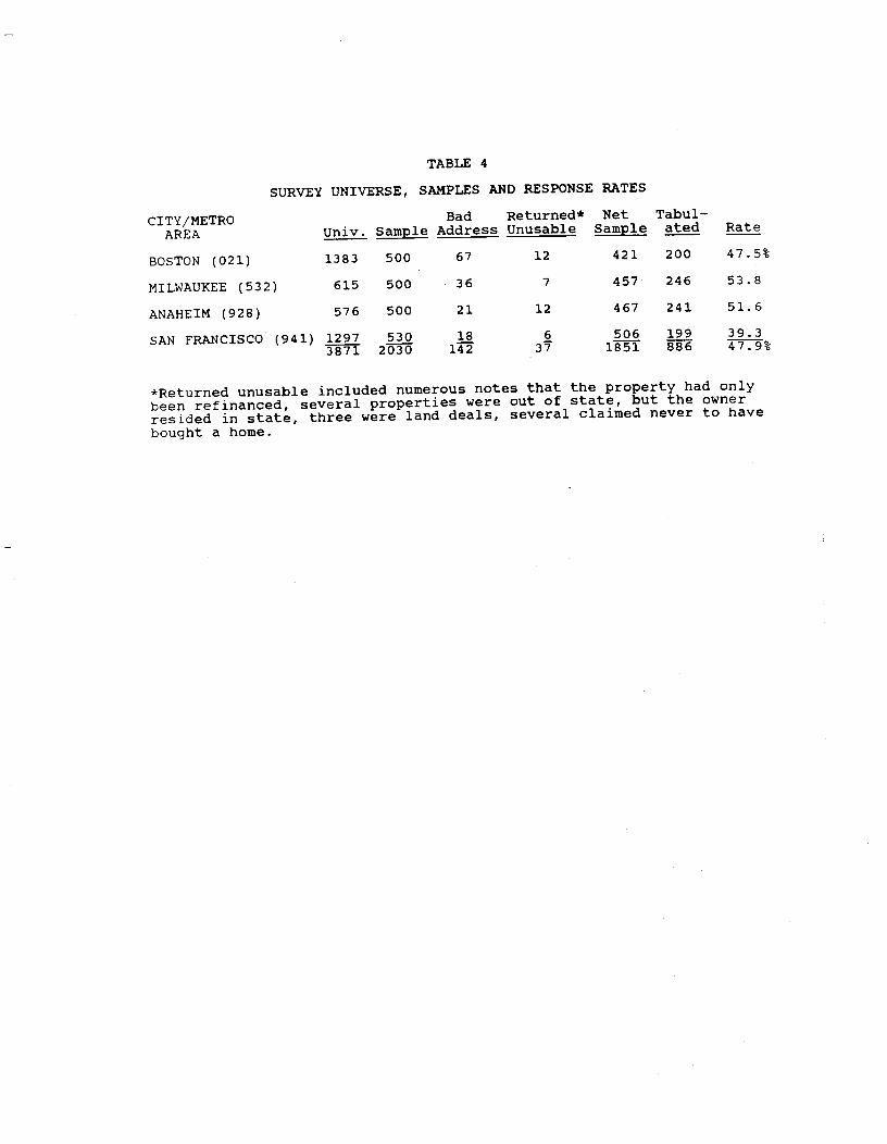
*Returned unusable included numerous notes that the property had onlybeen refinanced, several properties were out of state, but the ownerresided in state, three were land deals, several claimed never to have

bought a home.

SURVEY UNIVERSE, SAMPLES AND RESPONSE RATES

CITY/METROAREA Univ.

BadSample Address

Returned*Unusable

NetSample

Tabul-ated Rate

BOSTON (021) 1383 500 67 12 421 200 47.5%

MILWAUKEE (532) 615 500 36 7 457 246 53.8

ANAHEIM (928) 576 500 21 12 467 241 51.6

SAN FRANCISCO (941) 1297 530 18142

637

5061851

199886

39.347.9%

—7—

questionnaire with a personalized cover letter hand—signed by both authors.

The original mailing was sent on July 17 and 18. This was followed up with a

post card reminder mailed to the entire sample on July 26. A third mailing to

those who did not respond was sent on August 16 and 17. The third mailing

contained a duplicate questionnaire (for those who had misplaced the first)

and a new personalized cover letter. As an Incentive to participate, we

offered to send survey results to those who requested them.

A total of 142 surveys (7 percent) were returned "delivery attempted ——

not known" by the Post Office. Another 37 were returned by recipients but

were inappropriate for use in the survey. Among these were replies from

several who had only refinanced their homes, some who had bought land only,

others who had actually bought property out of state and a few who claimed to

have not been involved in a sale at all. With these excluded, the net sample

size was 1,851.

In total, 886 responses were coded and tabulated. Response rates were

above 50 percent In Milwaukee and Anaheim, close to 50 percent in Boston and

39.3 percent in San Francisco. Such response rates are about what we would

expect given the extensive follow up and personalized format. The

questionnaire was long and fairly detailed, taking close to half an hour to

complete, but the subject of the questionnaire was likely to be of interest to

recent home buyers.

The questionnaire

We did some pre—test interviews of a small number of home buyers In the

cities in our sample. He used some of their responses as the base for adding

questions to the survey.

—8—

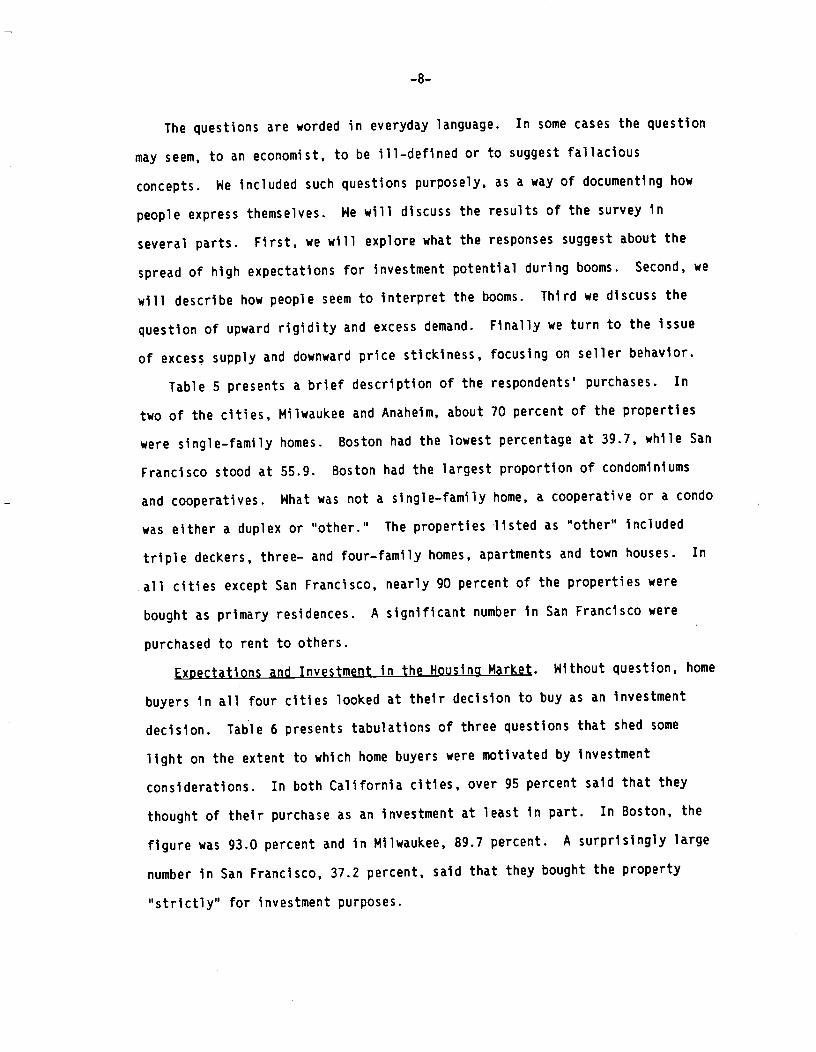
The questions are worded in everyday language. In some cases the question

may seem, to an economist, to be ill—defined or to suggest fallacious

concepts. We Included such questions purposely, as a way of documenting how

people express themselves. We will discuss the results of the survey in

several parts. First, we will explore what the responses suggest about the

spread of high expectations for Investment potential during booms. Second, we

will describe how people seem to Interpret the booms. Third we discuss the

question of upward rigidity and excess demand. Finally we turn to the Issue

of excess supply and downward price stickiness, focusing on seller behavior.

Table 5 presents a brief description of the respondents' purchases. In

two of the cities, Milwaukee and Anaheim, about 70 percent of the properties

were single—family homes. Boston had the lowest percentage at 39.7, whIle San

Francisco stood at 55.9. Boston had the largest proportion of condominiums

and cooperatives. What was not a single—family home, a cooperative or a condo

was either a duplex or "other." The properties listed as "other" Included

triple deckers, three— and four—family homes, apartments and town houses. In

a11 cities except San Francisco, nearly 90 percent of the properties were

bought as primary residences. A significant number in San Francisco were

purchased to rent to others.

ExDectations and Investment in the Housina Market. Without question, home

buyers in all four cities looked at their decision to buy as an investment

decision. Table 6 presents tabulations of three questions that shed some

light on the extent to which home buyers were motivated by Investment

considerations. In both California cities, over 95 percent said that they

thought of their purchase as an investment at least in part. In Boston, the

figure was 93.0 percent and In Milwaukee, 89.7 percent. A surprisingly large

number in San Francisco, 37.2 percent, said that they bought the property

"strictly" for investment purposes.

TABLE 5

GENERAL DESCRIPTION OF SURVEY RESPONDENTS'HOME PURCHASES

SanAnaheim Francisco Boston Milwaukee

Single family homes 70.0% 55.9% 39.7% 71.1%

Condo or coop 22.1 20.5 43.7 11.4

First time buyer 35.8 36.2 51.5 56.9

Bought to live in as aprimary residence 88.4 72.7 92.0 88.2

Bought to rent to others 3.7 12.1 3.0 4.1

TABLE 6

Housing as an Investment(Percent of responses in each category)

Questions:

"In decidin9 to buy your property,did you think of the purchase as aninvestment?"

"It was a major consideration"

"In part"

"Not at all"

(N=238) (N=199)

56.3 63.8

40.3 31.7

4.2 4.5

"Why did you buy the hone that you did?" (N=238) (N=199)

"Strictly for investment purposes" 19.8 37.2

(N=199) (N=246)

15.6 18.7

Boom Markets:San

Anaheim Francisco

PostBoom: Control:

Boston Milwaukee

(N2 00)

48.0

45.0

7.0

(N=243)

44.0

45.7

10.3

"Buying a home in today involves:" (N=237) (N=192) (N=l97) (N=237)

"A great deal of risk" 3.4 4.2 5.1 5.9

"Some risk" 33.3 40.1 57.9 64.6

"Little or no risk" 63.3 55.7 37.1 29.5

—9—

Clearly, one's wiflingness to pay for an asset depends in part on the

perceived degree of risk associated with it. Very few home buyers in any of

the four cities thought that the housing market involved a great deal of

risk. Even in Boston, where newspapers have been openly speculating about the

possibility of a crash, 37.1 percent said that buying a home involves little

or no risk. The degree of risk perceived is clearly lowest in the boom

markets. Rising prices seem to dampen fears, and that may well fuel the

boom. In Anaheim a full 63.3 percent said that their purchase was essentially

ri sk—free.

It is important to keep in mind from the outset that the sample is a

sample of actual home buyers. That is, the people who were surveyedwere the

ones who went out and bought homes in May. It can be assumed that they would

have significantly higher expectations than the general population of

Dotential home buyers. In addition, they are likely to have a lower

perception of risk than the general population of potential buyers. We did

not sample, and indeed could not have sampled, those who decided not to buy

because they were worried about future losses and risks.

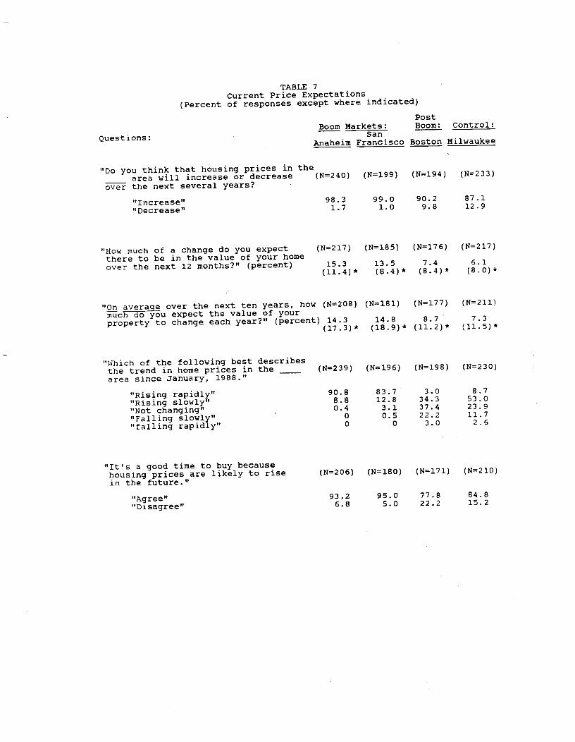
Table 7 presents responses to a number of questions designed to probe the

actual price expectations of buyers. First, virtually every buyer In our

California cities and the vast majority of buyers in Boston and Milwaukee

believe that prices will rise. As you would expect, those in the boom cities

are more optimistic than those in Boston and Milwaukee. Of 440 respondents

from California, only two said prices were falling and five thought prices

were not changing.

When asked how much they thought that their property would appreciate over

the next 12 months and over the next 10 years, the respondents' answers were

enormously varied. There were significant modes at 5, 10 and 15 percent in

Boom Markets:San

Questions: Anaheim Francisco

"Do you think that housing prices in thearea will increase or decrease

over the next several years?

"Increase"'I

"How much of a change do you expectthere to be in the value of your homeover the next 12 months?" (percent)

"Which of the following best describesthe trend in home prices in thearea since January, 1988."

"Rising rapidly""Rising slowly""Not changing""Falling slowly""falling rapidly"

(N=18 1)

14. 8

(l8.9)*

(N=177)

8.7(11.2) *

(N=2lfl

7.3(11.5) *

"It's a good time to buy becausehousing prices are likely to risein the future."

"Agree""Disagree"

93.2 95.0 77.86.8 5.0 22.2

TABLE 7Current Price Expectations

(Percent of responses except where indicated)

PostBoom: Control:

Boston Milwaukee

(N=240) (N=199) (N=l94) (N=233)

98.3 99.0 90.2 87.11.7 1.0 9.8 12.9

(N=2l7) (N=185)

15.3 13.5(l1.4)* (8.4)*

(N=l76)

7.4(8.4)*

"On average over the next ten years, how (N=208)much do you expect the value of yourproperty to change each year?" (percent) 14.3

(17 .3) *

(N=2l7)

6.1(8.0) *

(N=239) (N=196) (N=198) (N=230)

8.8 12.8 34.3 53.00.4 3.1 37.4 23.9

0 0.5 22.2 11.70 3.0 2.6

(N=206) (N=180) (N=17l) (N=2l0)

84.815.2

Table 7 Continued

Questions:

Boom Markets:— SanAnaheim Francisco

PostBoom: Control:

Boston Milwaukee

"Housing prices are booming. Unless Ibuy now, I won't be able to afford a (N=200)hone later."

"A9ree""Disagree"

"There has been a good deal of excitementsurrounding recent housing pricechanges. I sometimes think thatI may have been influenced by it:

"In conversations with friends andassociates over the last few months,conditions in the housing market werediscussed:"

(N=167) (N=169) (N=l94)

79.5 68.9 40.820.5 31.1 59.2

27.872.2

"yes"I'

(N=230) (N=191) (N=181) (N=233)

54. 345.7

56.5 45.343.5 54.7

21.578.5

(N=238) (N=l95) (N=l98) (N=235)

"Frequently""Sometimes""Seldom""Never"

* Standard Deviations

39.0 55.1 50.238.29.7 12.1 25.18.0 4.7

—10—

all four cities for both questions. In California, there were significant

modes at 10, 15 and 20 percent. The average expected annual increase for

buyers in California was in the 15 percent range, while for Milwaukee and

Boston, the figures were roughly half as high.

Three questions probed whether expected price increases actually

influenced the decisions to buy. The answer seems to be an overwhelming

"yes." Even in Boston, 77.8 percent reported that it was a good time to buy

because prices were likely to rise in the future. For Milwaukee the figure

was 84.8 percent, while it was well over 90 percent In both California

cities. At least one—quarter of the buyers In all markets and at least

two—thirds of the California buyers expressed a fear of being unable to afford

to buy a home in the future. Over half of the buyers in the boom cities

worried that they might have been influenced by the excitement surrounding

recent housing price movements.

Finally, the enthusiasm expressed In the boom cities seems to have a

social basis. There is significantly more discussion among friends and

associates in the California markets surveyed.

Interpretations of Booms. A number of specific questions were designed to

probe people's interpretations of price movements and possible triggers that

changed their opinions. It is critical to distinguish between mob psychology,

excessive optimism and a situation in which a solid reason to expect price

increases exists. Since most people expressed a strong Investment motive, one

would assume significant knowledge of underlying market fundamentals. The

efficient markets hypothesis assumes that asset buyers make rational decisions

based on all available information and based on a consistent model of

underlying market forces.

—11—

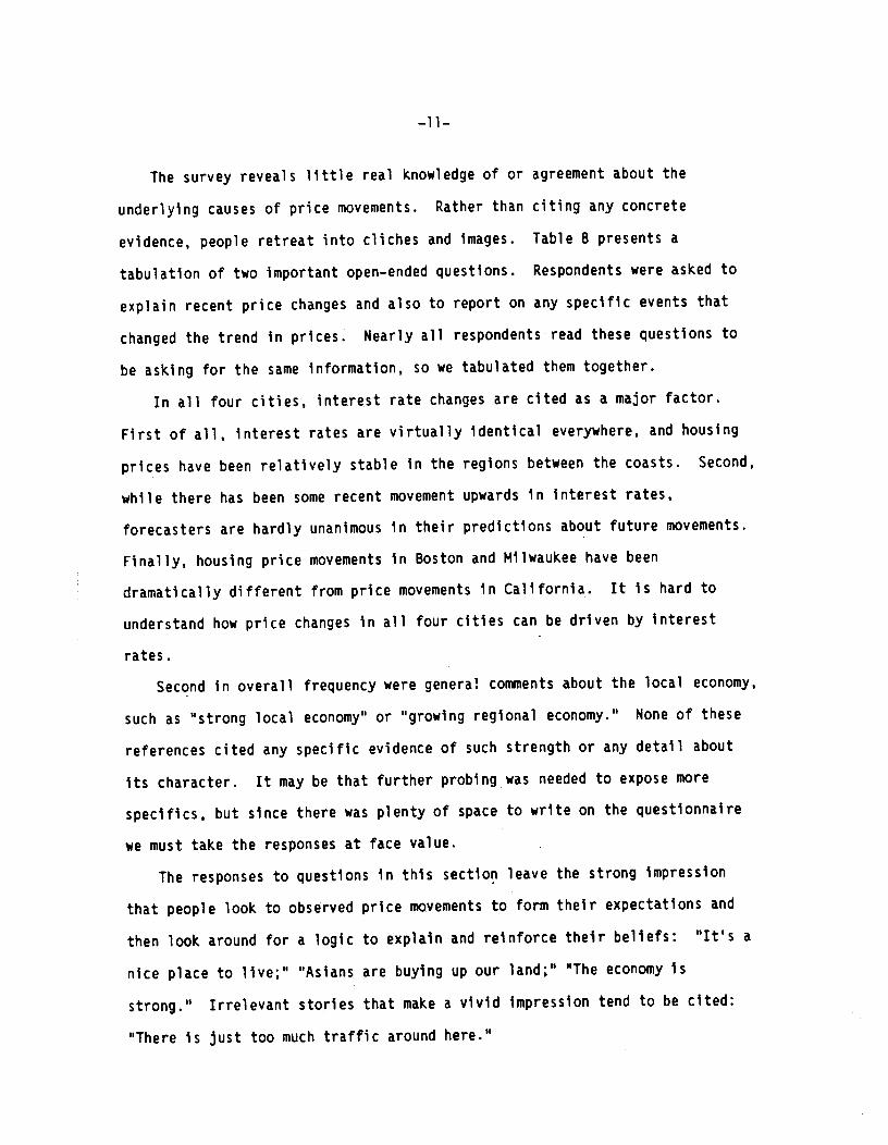
The survey reveals little real knowledge of or agreement about the

underlying causes of price movements. Rather than citing any concrete

evidence, people retreat into cliches and images. Table 8 presents a

tabulation of two Important open—ended questions. Respondents were asked to

explain recent price changes and also to report on any specific events that

changed the trend In prices. Nearly all respondents read these questions to

be asking for the same Information, so we tabulated them together.

In all four cities, interest rate changes are cited as a major factor.

First of all, interest rates are virtually Identical everywhere, and housing

prices have been relatively stable In the regions between the coasts. Second,

while there has been some recent movement upwards In interest rates,

forecasters are hardly unanimous in their predictions about future movements.

Finally, housing price movements In Boston and Milwaukee have been

dramatically different from price movements In California. It is hard to

understand how price changes in all four cities can be driven by Interest

rates.

Second in overall frequency were general comments about the local economy,

such as "strong local economy" or "growing regional economy." None of these

references cited any specific evidence of such strength or any detail about

Its character. It may be that further probing was needed to expose more

specifics, but since there was plenty of space to write on the questionnaire

we must take the responses at face value.

The responses to questions in this section leave the strong impression

that people look to observed price movements to form their expectations and

then look around for a logic to explain and reinforce their beliefs: "It's a

nice place to live;" "Asians are buying up our land;" "The economy is

strong." Irrelevant stories that make a vivid Impression tend to be cited:

"There is just too much traffic around here."

TABLE 8Popular Themes Mentioned in Interpreting Recent Price Changes

"What do you think explains recent changes in home pricesin _____? What ultimately is behind what's going on?

"Was there any event or events in the last two years thatyou think changed the trend in home prices?"

(Figures are percent of total Post

tabulated questionaireS by !2 Markets: Boom: Control:

city)San

Anaheim Francisco Boston Milwaukee

References to fundamentals:

National:Interest rate changes 31.7 39.5 24.5 27.0

Stock market crash 1.7 2.1 25.0 2.0

Demographics — baby boom 1.3 5.1 4.0 1.2

Tax law changes 1.3 4.1 3.0 2.0

Other national economic changes 1.7 5.1 8.5 2.9

Regional:Region is a good place to live 16.7 17.9 6.0 2.4

Immigration or population change 20.4 8.2 11.0 2.4

Asian investors 2.9 27.2 0 0

Asian immigrants 2.1 13.8 .5 0

Income growth 2.5 1.5 2.0 1.2

Anti—growth legislation 10.8 3.1 0 0

Not enough land 7.5 18.5 2.0 0.4

Local Taxes 2.9 0 4.0 9.8

Increasing Black population 0.4 0 0 6.6

Rental Rates and Vacancies .8 2.6 6.5 2.0

Traffic congestion 3.8 7.2 0 0

Local economy — general 25.4 4.6 29.5 18.4

Psychology of the Housing Market (a) 5.4 7.1 18.0 0.8

Quantitative evidence (b) 0 0 0 0

No answer 15.8 17.9 20.0 18.4

Notes to Table 8: To tabulate this open ended 9uestiOfl, 60 questionairesfrom each of two cities, Anaheim and San Francisco, were independently coded

by two coders. In addition, 60 questionaireS from the Boston sample werecoded by three coders. Intercoder reliability was tested by calculating thesimple correlation coefficient between the raw number of responses in eachcategory across coders. The correlation for Anaheim was .986 and for SanFrancisco .969. For Boston, three coefficients could be calculated: .953,.976 and .985. For cities used in the reliability test, the final score in

each catecory is the simple average across coders. The remainingquestionaires were coded by just one coder.

Notes to Table 8 Continued.

(a) Any reference to panic, frenzy, greed, apathy, foolishness, excessiveoptimism, excessive pessimism or other such factors were coded in thiscategory.

(b) Coders were asked to look for any reference at all to any numbersrelevant to future supply or demand for housing or to any professionalforecast of supply or demand. The numbers need not be presented aslong as the respondent seems to be referring to such numbers.

—12—

Among the most popular cliches were "The region Is a good place to live"

and "there is not enough land." Neither of these Is news and neither could

explain a sudden boom. We also asked exDlicitlv whether the boom was due to

the area's being a desirable place to live, and whether the real problem was

that there was not enough land available (table 9). (We asked these questions

because we had observed In pretesting telephone interviews that people in boom

cities tended to say this.) Respondents In boom cities very largely answered

"yes" to these questions. We were careful to ask the open—ended questions at

the beginning of the questionnaire and the explicit ones at the end to ensure

that we did not suggest answers. It should be noted, moreover, that it is one

of the strengths of our method that the same questionnaire was distributed in

the different cities. Very few people mentioned these cliches In Milwaukee.

Most participants in housing markets do not attribute market events to the

psychology of other investors. We see from table 8 that "psychology of the

market" was mentioned by housing market participants in fewer than 10 percent

of the responses, except for Boston where the figure was 18 percent. We also

asked explicitly whether respondents preferred to describe their own theory

about recent trends as one about psychology or one about economic fundamentals

(table 9). In all four cities fewer than a quarter picked psychology. This

is also consistent with evidence in Pound and Shiller (1987) about

institutional investors In corporate stocks, most of whom thought that prices

were driven by fundamentals, even in a stock whose price had boomed and had

high price—earnings ratios. However, a similar question was put to investors

right after the stock market crash of October 1987, and the answers were quite

different. About two—thirds of both individual and Institutional investors In

the United States thought the crash was due to market psychology (Shiller

1987), while three—quarters of iapanese institutional investors thought the

TABLE 9Buyers' Interpretation of Recent Events(Percent of respondents in each category)

PostBoom Markets: Boom: Control:

Questions: SanAnaheim Francisco Boston Milwaukee

"In a hot real estate market, sellersoften 9et more than one offer on the daythey list their property. Some are evenover asking price. There are alsostories about people waiting in line tomake offers. Which is the best (N2l0) (N=177) (N=176) (N=211)explanation?"

"There is panic buying, and pricebecomes irrelevant." 73.3 71.2 61.4 34.6

"Asking prices have adjusted slowlyor sluggishly to increasing demand." 26.7 28.8 38.6 65.4

"Housing prices have boomed inbecause lots of people want toTIVe (N2l0) (N=178) (N=181) (N=l93)here."

"Agree" 98.6 93.3 69.6 16.1"Disagree" 1.4 6.7 30.4 83.9

"The real problem in _____ is thatthere is just not enough land (Nl97) (N=l74) (N=168) (N=l92)available."

"Agree" 52.8 83.9 54.2 17.2

"Disagree" 47.2 16.1 45.8 82.8

"When there is simply not enoughhousing available, price becomes (N=197) (N=l65) (N=17l) (N=l93)unimportant."

"A9ree" 34.0 40.6 26.9 20.7"Disagree" 66.0 59.4 73.1 79.3

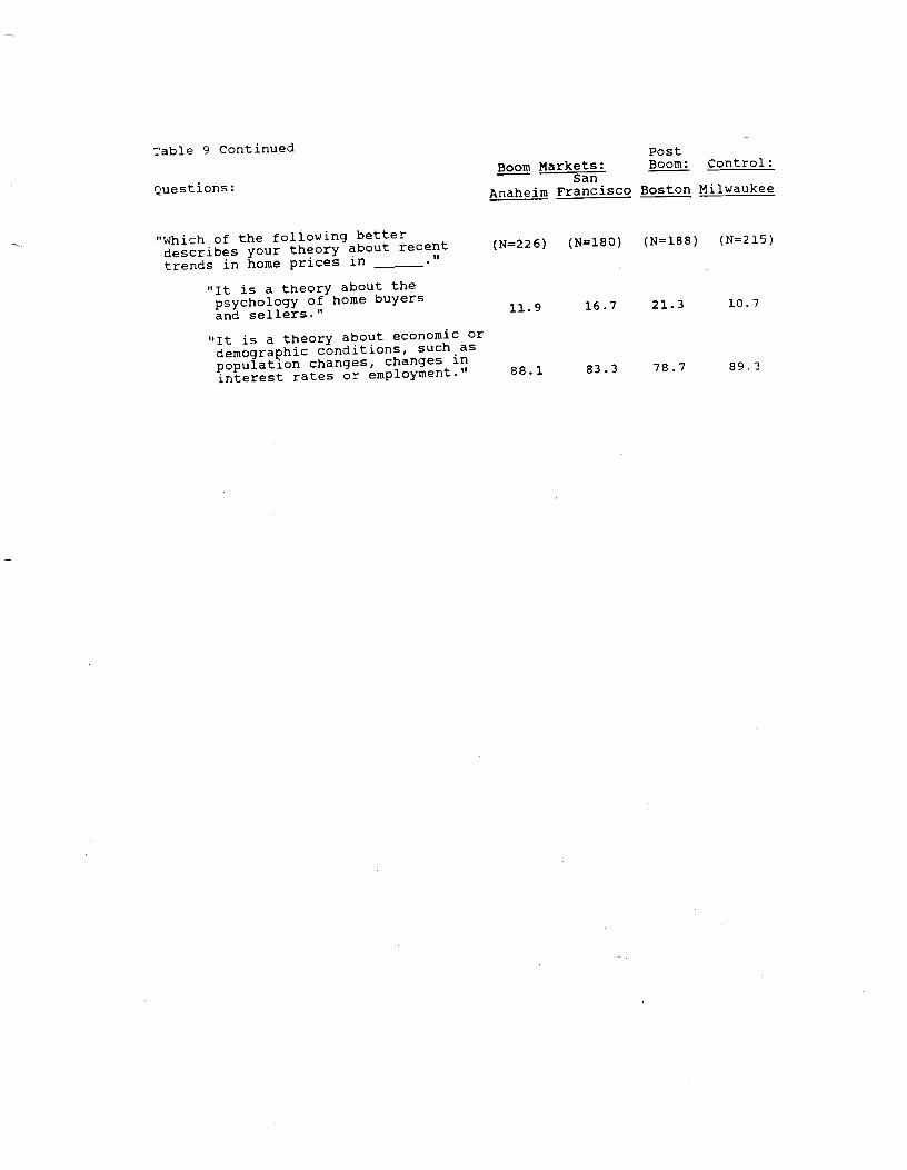
Table 9 Continued PostBoom Markets: Boom: Control:

QuestioflSSan

Anahei Francisco Boston Milwaukee

"which of the following betterdescribes your theory about recent

(N=226) (Nl80) (N188) (N=215)trends in home prices in _."

"It is a theory about thepsychology of home buyersand sellers."

11.9 16.7 21.3 10.7

"It is a theory about economic ordemographic conditions, such aspopulation changes, changes ininterest rates or emplOyment." 88.1 83.3 78.7 89.3

—13-.

crash was due to market psychology (Shfller, Konya and Tsutsui 1988). Perhaps

popular boom theories emphasize fundamentals as causes of upward price

movements (despite the fact that irrational behavior is thought to be

present), while sudden crashes are thought to be due to panic.

An especially striking feature of the coded answers In table 8 Is that not

a single respondent referred to explicit quantitative evidence relevant to

future supply of or demand for housing. We did not ask explicitly for such

evidence, but among 886 responses one would expect some to volunteer such

evidence if it figured prominently in their views.

Excess Demand and Upward Rigidity in Asking Prices. In boom cities,

newspaper accounts feature stories of homes that sold well above the asking

price, interpreting this phenomenon as evidence of investor frenzy or panic.

Recall the examples of such newspaper accounts from our discussion of the

current boom In California. The view that excess demand Is evidence of

Investor panic is also very popular among market participants in the boom

cities, as the last question in table 9 indicates. It Is likely that the

local media had some success in spreading the notion that prices above asking

prices are evidence of panic, since this view was much more common in the boom

cities than in the control city.

The news media seem to exaggerate the importance of such sales above

asking price. In fact, houses selling above the asking price were reported in

all our cities (table 10), so the fact that a newspaper reporter can find

examples is not much evidence of a boom market. The incidence of such sales

was significantly higher In the boom cities as in our control city, but was

still only about 6 to 10 percent. The prevalence of such examples Is better

at discriminating between boom and post—boom cities; fewer than 1 percent of

houses In our sample sold above the asking price In Boston.

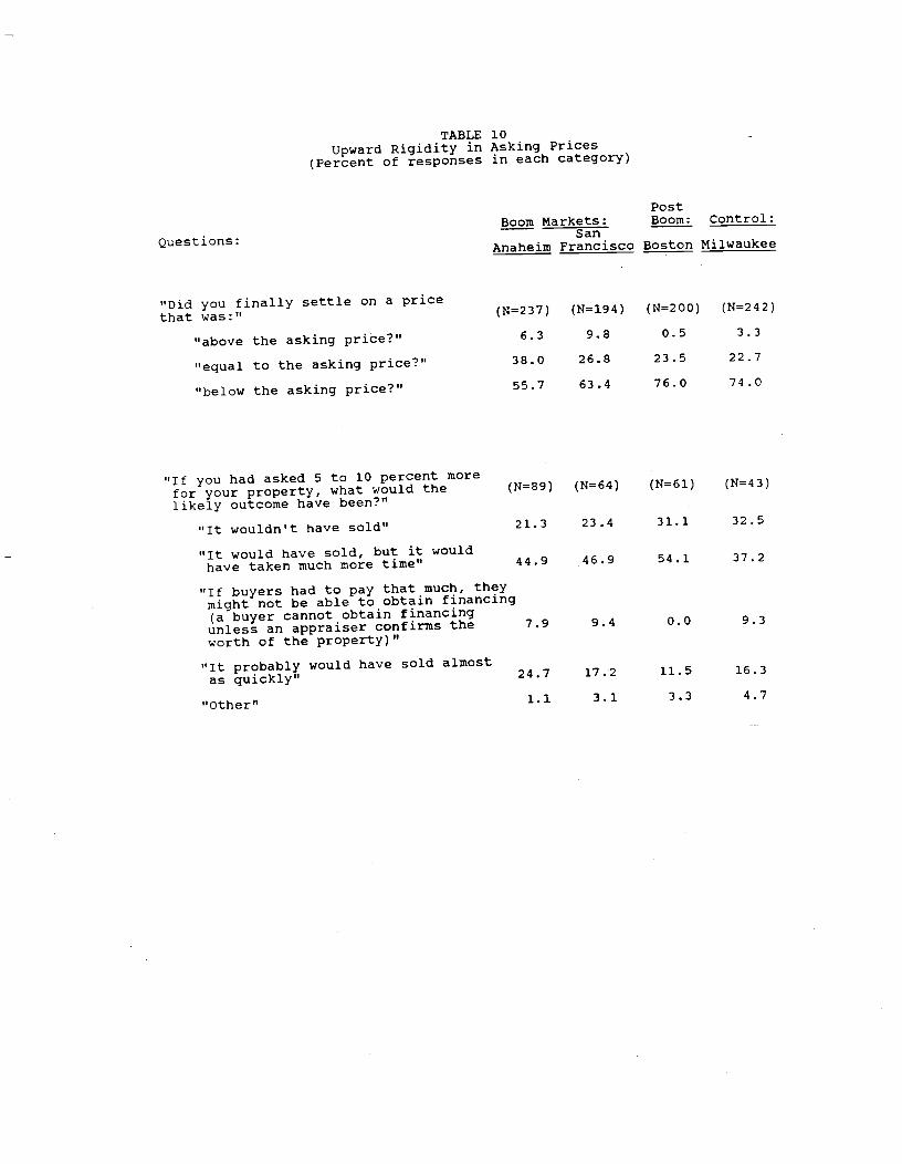
TABLE 10Upward Rigidity in Asking Prices

(Percent of responses in each category)

PostBoom Markets: Boom: Control:

Questions:San

Anahe Francisco Boston Milwaukee

"Did you finally settle on a pricethat was:"

"above the asking price?"

"equal to the asking price?"

"below the asking price?"

"If you had asked 5 to io percent morefor your property, what would thelikely outcome have been?"

"It wouldn't have sold"

"It would have sold, but it wouldhave taken much more time"

"If buyers had to pay that much, theymight not be able to obtain financing(a buyer cannot obtain financingunless an appraiser confirms theworth of the property)"

"it probably would have sold almostas quickly"

"Other"

6.3 9.8 0.5 3.3

38.0 26.8 23.5 22.7

(N=89) (N=64) (N=61) (N=43)

21.3 23.4 31.1 32.5

44.9 46.9 54.1 37.2

7.9 9.4 0.0 9.3

24.7 17.2 11.5 16.3

1.1 3.1 3.3 4.7

TABLE 10 continued

PostBoom Markets: Boom: Control:

Questions: SanAnaheim Francisco Boston Milwaukee

"If you answered that it would have soldalmost as quickly, which of the followingexplains why you didn't set the pricehigher (you can check more than one)" (N=37) (N=22) (N=26) (N=l6)

"The property simply wasn't worththat much" 32.4 27.3 38.5 25.0

"It wouldn't have been fair to set itthat high; given what I paid for itI was already getting enough." 16.2 22.7 15.4 31.3

"I simply made a mistake or got badadvise; I should have asked more" 21.6 18.2 19.2 25.0

"Other" 29.7 31.8 26.9 18.8

"In the six months prior to the timeyou first listed your property, didyou receive any unsolicited calls froma real estate agent or anyone else (N=89) (N=6l) (N=62) (N=48)about the possibility of selling yourhouse?"

"yes" 71.9 59.0 38.7 52.1

"No" 28.1 41.0 61.3 47.9

"Approximate Number" 8.7 5.0 3.9 2.7(l0.9)* (2.6)* (3.l)* (l.6)*

* Standard Deviations

-14—

Ne also sought evidence why some sellers did not raise their asking price

more (table 10). Those who thought they might have asked more often agreed

that notions of intrinsic worth or fairness played a role in their decision.

Real estate agents in the boom cities told us that, because of the excess

demand situation, they found It profitable to spend more time soliciting

listings, rather than showing houses to potential buyers. The responses to

the last question in table 10 largely confirm that real estate agents were

behaving as this would suggest.

Excess SUDD1V and ppwnward Rigidity In Asking Prices. A third important

aspect of behavior in housing markets Is seller behavior In post—boom markets

or generally soft markets. There is a good deal of worry that these booms

will end, as most stock market booms end, in collapse. If, indeed, what we

are observing in Orange County and San Francisco can appropriately be called

"bubbles," won't they inevitably burst?

One theory holds that housing prices are downwardly rigid, and that this

rigidity is likely to prevent major real estate collapses In the absence of a

general economic collapse. Significant reasons exist to predict such

rigidity. First, the housing market is very different from the stock market.

In the stock market, people can exit their equity positionsquickly and almost

without cost. The analog of a Treasury Bill in the housing market Is moving

to a rental unit. For those with considerable equity this would mean paying

large capital gains taxes and a 6 percent brokerage fee, as well as putting up

with the aggravation of a move. Thus, the transactions costs are very large.

Second, investors have an alleged psychologicaldisposition to sell their

winning investments (to have the satisfaction of getting their money), and to

hold on to losing investments (to avoid the pain of regret; see Shefrln and

Statrnan 1985). Ferris, Haugen and Hakhija 1988have found evidence for this

—15—

"disposition effect" by documentation that the volume of trade in stock whose

value has declined is lower than in stocks that have increased in value.

In addition, the popular impression is that past experience has shown that

waiting may pay off, perhaps the best example being California in 1981. After

four years of boom, housing prices stopped rising. While it is clear that

some people lost money in the real estate market, many simply decided to wait

It out; the number of transactions dropped to very low levels, and median

price never fell in nominal terms. Since 1983, prices have again been on the

rise.

Table 11 presents evidence on seller behavior in markets with excesss

supply. All respondents were asked to react to the first statement on table

U. Nearly 70 percent of respondents in California agreed with the statement

that the best strategy in a slow market is to hold on until you get what you

want. In Boston and Milwaukee more than half agree.

The remaining questions were asked of those who had sold or tried to sell

a property immediately prior to buying the one that they bought. This

relatively small sample is likely to be a biased sample of all sellers.

Recall that these sellers are the ones who actually bought new homes. If a

seller was unable to sell her house, did not lower her price, and ultimately

decided not to buy a new house, she Is not In our sample. Thus, those who

were at least somewhat flexible are likely to be over—represented.

Buyers who had sold or tried to sell a home prior to buying their present

unit were 39.6 percent of the total respondents in AnaheIm, 32.6 percent in

San Francisco, 32.8 percent In Boston, and 21.3 percent In Milwaukee. Since

the vast majority of this group (over 90 percent in all cities except

Milwaukee where the figure was 84.3 percent) had actually sold their

properties, the only way to probe the issue was with a hypothetical question.

TABLE 11Excess Supply and Downward Rigidity in Asking Prices

(Percent of responses in each category)

PostBoom Markets: Boom: Control:

Questions:San

Anaheim Franc22 Boston Milwaukee

"Since housing prices are unlikely todrop very much, the best strategy in

a slow market is to hold on until you (N=174) (N=l48) (N=160) (N=l80)

get what you want for a property"

"Agree"69.0 69.6 57.5 50.6

"Disagree"31.0 30.4 42.5 49.4

"If you had not been able to sell yourproperty for the price that you (N=88) (N=62) (N=6l) (N=43)

received, what would you have done?"

"Left the price the same and waitedfor a buyer knowing full well that 42.0 38.7 32.8 32.6

it might take a long time."

"Lowered the price step by stephoping to find a buyer." 20.5 38.7 42.6 20.9

"Lowered the price till I found a

buyer."4.5 3.2 4.9 7.0

"Taken the house off the market." 18.2 17.7 11.5 27.9

"Other" (a)14.8 1.6 8.2 11.6

"If you responded that you woul havelowered your price, is there a limitto how far you would have gone if the (N=33) (N=38) (N=29) (N=l6)

property still hadn't sold?"

"Yes" 81.8 78.9 93.1 87.5

Table 11 Continued

PostBoom Markets: Boom: Control:

Questions:San

Anaheim Francisco Boston Milwaukee

"If you answered yes to the abovequestion, can you say how you arrived (N24) (N=28) (N=21) (N=l0)

at that limit" (Open ended)

Based on what I paid 29.2 21.4 19.0 30.0

Based on price of another homethat I want to buy 33.3 35.7 38.1 20.0

Based on what other similar homeshave sold for 37.5 42.9 42.9 50.0

"If your property did not sell,presumably it would have if you hadlowered your asking price more. Ifyou considered doing so but decided (N=19) (N=18) (Nl3) (N=13)

riot to can you say why?"

"My house is worth more thanpeople seem to be willing to 15.8 11.1 7.7 38.5

pay right now."

"I can't afford to sell at alower price" 26.3 33.3 23.1 15.4

"By holding out, I will be ableto get more later." 31.6 44.4 15.4 7.6

"Other." (b) 26.3 11.1 53.9 38.5

(a) The most frequently mentioned "other" categories were company buy outprovisions and that sellers would rent the property out.

(b) Many of the "other" responses made reference to time, i.e., "I was inno hurry," "I was not anxious about selling" or "I had no need to sell."

—16—

We asked, "If you had not been able to sell your property for the price that

you received, what would you have done?" Only a very small fraction said that

they would lower their price until they found a buyer —— the market—clearing

solution.

A significant percentage (between 20 and 40 percent) In each city said

that they would lower the price step by step, looking for a buyer. However,

when probed further, more than three quarters in all cities reported that

there was a limit to how far they would drop the price: Surprisingly the

figures were highest in Boston and Milwaukee, 93.1 percent and 87.5 percent

respectively. Most of them seemed to have some knowledge of what comparable

homes had sold for, and they did not want to sell for less.

The "other" category in the second question reported in table 10 reveals

two additional sources of downward rigidity. Several respondents mentioned

that their employer had a buy—out program for employees who could not sell.

What they really meant was a buy—out plan for employees who could not sell at

the price that they wanted to get. A number of others reported simply renting

out their first property.

Finally, the small group of sellers who had not sold their properties were

asked why they did not simply drop their price. Some of the same notions of

fairness or Intrinsic worth that played a role in the upward rigidity studied

above appear to play a role here. Others said they could not afford to sell,

and still others expressed optimism that they could sell at a higher price

eventually.

IV. Interpretations and Conjectures

What have we learned about sources of the booms that from time to time

appear in local housing markets? Evidence in this paper supports the view

—17—

that the suddenness of booms has to be understood in terms of investor

reactions to one another, to past price increases, or to other evidence of

boom markets, rather than to economic fundamentals. Of course, we did not

look at data on fundamentals in this paper, and the paper that one of us did

on the Impact of fundamentals on city housing prices (Case 1986) is certainly

not the last word on the subject. But we have in this paper provided some

evidence that investors in housing markets do not know fundamentals. They

tend to interpret events in terms of hearsay, cliches, and casual

observations. Moreover, we have seen that investment motivations are high on

their list of incentives, and that home buyers in booms expect still more

appreciation of housing prices and are worried about being priced out of the

housing market in the future. It is certainly plausible that expectations

heavily influence the prices people are willing to pay in these markets.

Because these expectations do not appear to make much sense except as

extrapolations of past price changes, we cannot expect prices to be rationally

determined.

But what starts a housing boom; why does It occur in one year and not

another? We asked home buyers what they thought was going on, and whether

they could name an event that they thought changed the behavior of housing

prices. The most popular answer In all cities was a change in interest rates,

but interest rates do not differ much across cities and so cannot be the

explanation of the differing price behavior. Moreover, Interest rates were

cited as the cause of the boom in California and as the cause of stagnation in

Boston. For the most part, respondents did not produce another event. The

most plausible—sounding event In Anaheim (proposed anti—growth legislation)

was quite different from the most plausible—sounding event in San Francisco

(the entrance of Asian investors into the market), and yet the pattern of

—18—

price changes was similar in the two cities. The events may instead be

after—the—fact rationalizations of the price movements, just as the October

1987 stock market crash was brought up mainly in Boston, where an explanation

of a slump was needed.

The trigger Is apparently an event or sequence of events not observed by

most home buyers. Since the ultimate trigger is not the factor In the minds

of investors, it could even be something that was not observed by .ay

Investors, except through price. For example, demographicchange or income

growth could cause an initial price Increase, to which home buyers reacted.

Perhaps home buyers in California in 1987 and 1988 were also more primed to

react to a price Increase, having heard stories ofthe boom in the Northeast.

Another puzzle concerns the slowness of the booms: Why do booms extend

over years, and not accelerate and terminate very quickly? Our survey results

offer only marginal help In conjectures regardingthis question. The notion

expressed by some investors that they were motivated by a sense of intrinsic

worth and comparisons with past prices may suggest that there is a

psychological resistance to very rapid priceincreases. It is of course true

that there are barriers to professsionai speculators entering and closing off

profit opportunities in the market for single—family homes; that Is why we

were not surprised to find persistencein price changes in our earlier study

of the efficiency of housing prices (Case and Shiner 1989). Ordinary

Individuals, who are not Investment professionals, should be expected to take

more time before investing. Such action may involve a change in living

arrangements and may well take months or years.

Respondents were somewhat Inconsistent in their reporting of their

impression that psychological factors wereresponsible for the booms. We saw

that about half of respondents in boom cities thought they themselves were

—19—

influenced by the excitement, and that most interpreted houses selling above

asking prices as evidence of panic. Yet other evidence in tables 8 and 9

indicates that most investors do not think that market psychology is the best

explanation for booms, citing fundamentals instead. Perhaps we should

conclude that social psychology is an important factor in the transmission of

booms, but that individuals' perceptions of the psychology of others are less

so.

The proportion of homes that sell above the asking price Is quite low in

all cities. Apparently newspapers feature such stories in boom cities because

they are perceived as relevant to the big story of area—wide price increases.

In a city not experiencing such price increases, such occurrences are more

likely to be interpreted as evidence of simple errors In setting the asking

price, and are not thought to be particularly newsworthy.

If such occurrences reflect mistakes by a small minority of sellers in

setting the asking price, then it is to be expected that such errors will

occur more frequently in cities that are currently experiencing Increases if

some sellers are slow to adjust their price. Perhaps occurrences of sales

price above asking price ought to be Interpreted as nothing more than that.

On the other hand, some of the answers reported in table 10 suggest that

notions of a fair price or of intrinsic worth may also play a role in the

sluggishness of price changes. Kahneman, Knetsch and Thaler (1987) have

documented the Importance of notions of fairness In many economic decisions.

The same notions of fairness arise also in answers to questions as to why

those who had trouble selling houses did not cut their prices more.

Evidence of price rigidity appeared to be more significant In falling

markets than in rising markets. Only about 5 percent of the respondents in

the post—boom city Boston who had not sold their former property said they

—20—

would continue to lower the price until a buyer was found. One possible

explanation of the downward rigidity in housing prices comes from the prospect

theory of Kahneman and Tversky (1979). In their theory, losses and gains are

viewed very differently, and the point from which individuals measure whether

they have made a gain or loss may be determined by the frame of reference that

attracts their attention.3

The Regret theories of Bell (1982) and Loomis and Sugden (1982) have

similar implications. However, as we saw above, other Interpretations of the

rigidity are possible. Popular impressions as to the likely course of future

prices are also at work here. The fact that a high a proportion of home

buyers in all cities thought there was little risk in the housing market

reflects a popular view that one cannot lose in this market; houses are always

a safe investment, so long as one holds out long enough.

Another reason chosen by those who could not sell was that "I can't afford

to sell at a lower price." Since all of the respondent sellers had

subsequently bought another house, it is likely that an important factor in

this judgment was the price of the other house they bought. If all real

estate prices are too high, one may find it difficult to cut the asking price

on one's own house, since one cannot coordinate this price cut with the seller

of the house one wishes to purchase. Part of the problem in downward rigidity

of housing prices may then be a coordination problem of the kind that economic

theorists have stressed in other contexts.4 If we could all agree at once

to cut the prices of our houses, we might all be happy, but I can't be the

first one to cut.

All these reasons for downward rigidity in prices may be interrelated. If

the coordination problem prevents prices from falling, this creates an

impression that they should not fall and therefore an impression that it pays

—21—

us to hold out; this impression heightens the regret experienced If one cuts

price.

Conclusions

All of this suggests a market for residential real estate that Is very

different from the one traditionally discussed and modeled In the literature.

In a fully rational market1 prices would be driven by fundamentals such as

income, demographic changes, national economic conditions and so forth.

Investors In such a market would use all available Information on potential

changes in fundamentals to forecast future price movements, making prolonged

prIce swings impossible and profit opportunities rare. Resources including

access to popular regions would be efficiently allocated.

The survey results presented here and actual price behavior together

sketch a very different picture. While the evidence is circumstantial, and we

can only offer conjectures, we see a market driven largely by expectations.

People seem to form their expectations on the basis of past price movements

rather than any knowledge of fundamentals. This increases the likelihood that

price booms will persist as home buyers In essence become destabilizing

speculators.

He also found significant evidence that in the absence of a severe

economic decline, housing prices are inflexible downward. Combined with

upward volatility, this inflexibility has produced a ratcheting effect in some

boom cities with complicated distributional consequences, as owners gain at

the expense of non—owners at all levels of income.

At this point we are not prepared to offer or even speculate about

possible policy conclusions. We only hope that further research will help

shed more light on this still puzzling market.

Footnotes

*Karl E. Case is Professor of Economics, Hel'Iesley College, and Visiting

Scholar, Federal Reserve Bank of Boston. Robert 3. Shiller is Professor of

Economics, Yale University, and Research Associate, National Bureau of

Economic Research.

*The authors are Indebted to the survey respondents who took valuable time

to complete the questionnaire. We also want to thank Alicia Munnell, Kenneth

Rosen, Jeremy Siegel and participants atthe Sage Foundation Conference on

Behavioral Finance as well as seminar participants at Harvard and the

University of Pennsylvania for helpful discussions. We are grateful to Anne

Kinsella at the Boston Federal Reserve Bank and Larry Baldwin at Wellesley for

masterful programing to help get the survey out and the returns coded. Paula

Andres, Jie Cao and Janet Hanousek worked very hard as research assistants.

Funding was provided by the Federal Reserve Bank of Boston, the National

Science Foundation, and Hellesley College.

1See Drexier, Schwartz, and Grelner (1988).

2The Boston Glob, February 17, 1988, p. Bl.

3Kahneman and Tversky write that "This analysis suggests that a person

who has not made peace with his losses is likely to accept gambles that would

be unacceptable to him otherwise" (1979, p. 287).

4For example, Keynes's theory of the downward rigidity in wages in a

depression was that "since there is, as a rule, no means of securing a

simultaneous and equal reduction of money—wages In all Industries, It Is in

the interest of all workers to resist a reduction in their own particular

case" (1936, p. 264).

References

Bell, David E.. 1982. "Regret in Decision Making Under Uncertainty."Operations Research, voL 9, September—October, pp. 961—8L

Case, Karl E. 1986. "The Market for Single Family Homes in Boston," New England

Economic RevIew, May/June.

Case, Karl E., and Robert J. ShIller. 1987. "Prices of Single—Family HomesSince 1970: New Indexes for Four Cities." New England Economic Review,

September/October.

_________ 1989. "The Efficiency of the Market for Single—Family Homes." Iti....

m.e.rian Ecnom1c Review, forthcoming, March.

Diliman, Don A. 1978. Hail and Telephone Surveys: The Total Design Method.John Wiley and Sons.

Drerier, Peter, David C. Schwartz, and Ann Greiner. 1988. "What Every BusinessCan Do About Housing." Harvard Business RevIew September/October, p. 52.

Ferris, Stephen P., Robert A. Haugen, and Anil K. Makhlja. 1988. "PredictIngContemporary Volume with Historic Volume at Differential Price Levels ——

Evidence Supporting the Disposition Effect." The Journal of Finance, July.

Kahneman, Daniel, Jack L. Knetsch, and Richard Thaler. 1986. "FaIrness as aConstraint on Profit Seeking: Entitlements in the Market." The AmericanEconomic Review, vol. 76, No. 4, September, pp. 728—41.

Kahneman, Daniel, and Amos Tversky. 1979. "Prospect Theory: An Analysis ofDecision Under Risk." Econometrica, vol. 47, pp. 236—91.

Keynes, John Maynard. 1936. The General Theory of Employment. Interest andMoney. Harbinger: New York, 1964 edition.

Loomis, Graham, and Robert Sugden. 1982. "Regret Theory: An AlternativeTheory of Rational Choice Under Uncertainty." The Economic Journal, vol.

92, December, pp. 805—24.

Pound, John, and Robert 3. Shiller. 1987. "Are Institutional InvestorsSpeculators?" Journal of Portfolio Management, Spring, pp. 46—52.

Shefrin, Hersh, and Heir Statman. 1985. "The Disposition to Sell Winners TooEarly and. Ride Winners Too Long: Theory and Evidence." The Journal of

Finance, Vol. XL, No. 3, July, pp. 777—90.

Shiller, Robert J. 1987. "Investor Behavior in the October 1987 Stock MarketCrash: Survey Evidence." National Bureau of Economic Research Working

Paper No. 2446, November.

Shiller, Robert J., Fumiko Konya, and Yoshiro Tsutsui. 1988. "InvestorBehavior In the October 1987 Stock Market Crash: The Case of Japan."National Bureau of Economic Research Working Paper.